Nonperturbative quark-antiquark interactions
in mesonic form factors

Abstract

The existing theory of hard exclusive QCD processes is based on two assumptions: (i) $factorization$ into a hard block times light front distribution amplitudes (DA’s); (ii) use of perturbative gluon exchanges within the hard block. However, unlike DIS and jet physics, the characteristic momentum transfer $Q$ involved in the factorized block is not large enough for this theory to be phenomenologically successful. In this work, we revisit the latter assumption (ii), by explicitly calculating the instanton-induced contributions to the hard block, and show that they contribute substantially to the vector, scalar and gravitational form factors of the pseudoscalar, scalar and vector mesons, over a wide range of momentum transfer.

I Introduction

I.1 The main goals and plan of the paper

The field of hadronic physics going back to the pioneering theoretical and experimental works of the 1960’s, continues to be a field of active development till today. Remarkably, it remains still deeply divided along two conceptually different approaches.

One approach is focused on the nontrivial vacuum properties, with more specifically the central aspects of chiral symmetry breaking and confinement. The discovery of instantons and the development of numerical lattice gauge theory have put the Euclidean formulation of QCD at the center stage. The theory and phenomenology of multiple Euclidean correlation functions, became the primary source of information about quark-quark interactions. The inter-relation of perturbative and nonperturbative contributions in various channels, as a function of the distance between the operators, were clarified already in 1990’s (see e.g. a review Shuryak (1993)). Models, with “constituent quark” masses, confining and “residual” 4-fermion forces, provided a good description of most aspects of hadronic spectroscopy. More recently, the discussion has shifted to the properties of operators made of 4-, 5- and 6-quarks and their mixture with gluons.

Another approach is focused on partonic physics, with more specifically inclusive and exclusive reactions. The reader hardly needs to be reminded of the importance of deep inelastic scattering (DIS) and jet physics, where perturbatively calculated hard cross sections are assumed to factor out from the structure and fragmentation functions, which are empirically fitted to large sample of data. These functions, defined on a light front, are not readily amenable to an Euclidean formulation. The light front distribution amplitudes and functions of the lightest hadrons have been discussed in the context of the QCD sum rules Radyushkin (1994), bottom-up holographic models Brodsky et al. (2011), bound state resummations Chang et al. (2013), basis light front quantization Jia and Vary (2019); Shuryak (2019), and covariant constituent quark models Broniowski and Ruiz Arriola (2017); Petrov and Pobylitsa (1997); Anikin et al. (2001). Recently, an Euclidean formulation was put forth to extract the light front distributions from equal-time quasi-distributions Ji (2013); Ji et al. (2015). Its implementation on the lattice Zhang et al. (2017), and in the random instanton vacuum model Kock et al. (2020) have been reasonably successful, providing a first principle approach.

The theory of exclusive QCD reactions (the subject of this work) follows a similar reasoning, see the early works Brodsky and Farrar (1973); Chernyak and Zhitnitsky (1977); Radyushkin (1977). It is also based on two assumptions:

(i) the separation of scales, based on the assumption that the momentum transfer $Q$ (the scale in the “hard block”), is large compared to the typical quark mass and transverse momenta inside hadrons;
(ii) the “hard block” can be calculated perturbatively using gluon exchanges.

However, the theory based on these two assumptions is insofar not successful, as there remains a wide gap between the semi-hard domain of $Q$ in which experimental/lattice results are available and the “asymptotic” theory at $Q\rightarrow\infty$. (The latest lattice results with very fine lattices that we will discuss at the end of the paper are starting to fill this gap). The empirical values of the mesonic form factors times $Q^{2}$ are well above the one-gluon exchange predictions, even with (what we consider maximally possible) flat distribution amplitudes and higher twist contributions included.

This is not surprising, as there is an important difference between the scales in DIS and jet physics on one hand, and exclusive processes on the other. The former operates in the range $Q^{2}=10^{2}-10^{4}\,{\rm GeV}^{2}$, while the exclusive processes operates in a different range with $Q^{2}=2-10\,{\rm GeV}^{2}$ (sometimes referred to as a $semi-hard$ regime).

We accept the assumption (i) mentioned above: the $Q^{2}$ scale is indeed large compared to the typical squared transverse momentum $\langle p_{\perp}^{2}\rangle\sim 0.1\,{\rm GeV}^{2}$ within a hadron, or the constituent quark mass $M_{Q}^{2}\sim 0.1-0.15\,{\rm GeV}^{2}$. In the Breit frame description of the form factors, conventional “collinear” kinematics should still hold. So we still have a notion of a “hard block operator”, sandwiched between two wave functions.

Yet we do not accept the second assumption (ii), showing that at such momentum transfer $Q$, the nonperturbative quark interactions are $not$ at all negligible in comparison to gluon exchanges. Therefore a purely perturbative treatment of the “hard block” needs to be supplemented by calculations of leading nonperturbative contributions from first principles, and this paper makes the first steps in this direction.

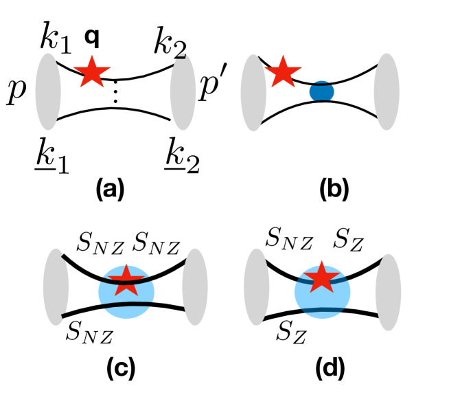
Figure 1: The perturbative one-gluon exchange diagrams: (a) explains our notations for momenta of quarks and mesons. The thin solid lines are free quark propagators, the red star indicates the virtual photon (or scalar) vertex, bringing in large momentum $q^{\mu}$, and the shaded ovals represent the (light-front) mesonic density matrices (distributions). The diagram (b) indicates a “Born-style contribution”, in which the gluon propagator is substituted by the Fourier transform of the instanton field. The diagrams (c,d) contain three propagators in the instanton background (thick lines). In (c) all of them are $S_{NZ}$, made of nonzero Dirac modes, while in (d) two of them are $S_{Z}$ made of quark zero modes. This last contribution will be referred to as the “’t Hooft-style term”.)

Among various exclusive reactions, the recent literature is focused mainly on decays of heavy quark mesons such as D- and B-mesons, much studied at electron colliders. However, in this work we restrict our analysis to only elastic form factors of $light$ mesons. We will consider two types of “hard blocks”, induced either by virtual photons or scalars. (Of course, scattering of Higgs bosons cannot be experimentally achieved, but it has been studied on the lattice, and it is rather interesting.)

Before we outline the content of this work, let us comment on other approaches aimed at the mesonic form factors. Instead of discussing on-shell light-cone distribution amplitudes, one may start with two- or three-point correlation functions, containing the electromagnetic current and two local currents with meson quantum numbers. One of them or both may carry large virtuality, in which case the three points probed are all close to each other. After evaluating the correlation functions in the deeply virtual regimes, one relates them to on-shell form factors via dispersion relations or QCD sum rules.

For the pion form factor these approaches can be split into two categories, based on the different pion currents used. The first one (e.g.Braun et al. (2000)) uses the $axial$ currents $(\bar{d}\gamma_{\mu}\gamma_{5}u)$, while the second one uses the pseudoscalar one $(\bar{d}\gamma_{5}u)$. Note that in the former both quarks carry the same chirality (LL+RR), while in the latter they carry opposite chiralities (LR+RL).

In the first category, the correlators are analyzed using the QCD sum rule methods, previously developed for the two-point axial current correlators. They make use of the operator product expansion (OPE) which assumes that the distances between the currents are small in comparison to the typical vacuum fields, represented by the gluon and quark condensates. The small-distance correlators are then connected to integrals over on-shell contributions using the pertinent spectral densities, with the pion plus the $A_{1}$ meson plus a “high energy continuum”. In the second category, the distances between the currents are also assumed to be small, but the calculation is based on the so called single-instanton approximation (SIA), see Forkel and Nielsen (1995); Blotz and Shuryak (1997); Faccioli et al. (2003); Braguta and Onishchenko (2004).

Instead of comparing the specific results of these works, we make a more general comment on the same ideas previously applied to the $two-point$ functions. Since the axial spectral density is known experimentally from $\tau$-lepton decays, these correlation functions are phenomenologically known (see e.g. analysis in Schäfer and Shuryak (2001) and many others). The OPE expressions may only be used at rather small distances $x<0.4\,{\rm fm}$, while the pion contribution becomes visible only at much larger distances $x>1\,{\rm fm}$. In between, the contribution of the $A_{1}$ meson dominates. Therefore we are very sceptical of the approach in the first category. (Note also that the “instanton liquid model” works at all distances, see Fig.2 in Schäfer and Shuryak (2001).)

The pseudoscalar two-point function is also known, and was calculated on the lattice in multiple works (see e.g. Negele (1997)). Unlike the axial case, here the pion contribution is large and dominant already at small distances $x\sim 0.3\,{\rm fm}$. It is also well reproduced by the single instanton contribution. Therefore, one should perhaps trust the accuracy of the approach in the second category (with the pseudoscalar currents) more. (The relevance of these comments to our work will be evident below, in the relative contributions of the mesonic distribution amplitudes (DA) with different chiral structure).

The outline of our paper is as follows: the next introductory section compares the magnitude of one-gluon exchange with a generic 4-fermion interaction of the Nambu-Jona-Lasinio type, to get an initial qualitative idea on the relative strength of the perturbative and nonperturbative effects. Clearly, the nonperturbative contributions will wane out at larger momentum transfer. This section also includes a subsection I.3 with a brief introduction to the salient instanton effects and their key parameters.

Since the paper contains a lot of technical details, not so important for a first reading, we decided to collect all the results for the pion, the rho vector meson, the scalar and gravitational form factors in section II. The actual calculations start from the perturbative ones in section III.1. They include the twist-2 and twist-3 contributions, most of which have been discussed in some form in the litterature for the vector form factors, but not in a fully quantitative manner.

As discussed in subsection III.6, these results can be generalized to a large set of effective 4-quark scattering operators, as a substitute for one-gluon exchange. A simple warm-up calculation of this kind consists in taking the Fourier transform of the instanton field instead of a gluon propagator, as discussed in section III.7. We do not consider such an approach internally consistent, and for this reason we will not include it in the ”results” section.

The core calculations of the instanton-induced effects are collected in section IV. We start by explaining an LSZ algorithm (short of a Hamiltonian formulation), whereby full multiple quark propagators in the instanton field are amputated from their trivial free propagation, and leading to hard block operators. We discuss separately the contributions to the propagators due the Dirac zero modes and the Dirac non-zero modes.

Section V contains a discussion of the mesonic light cone distribution amplitudes (DA’s), which are the wave functions integrated over transverse momenta. Following a brief review of the literature, we introduce the pion, rho and scalar meson amplitudes with different chiral structures, which we use consistently in the results of the calculations. The paper ends with a discussion section VI, in which the phenomenological and current lattice results about the mesonic form factors are compared. A number of Appendices are added to include more technical details of the calculations.

I.2 Comparing the one-gluon exchange with the 4-fermion interaction of the Nambu-Jona-Lasinio model

Historically, the 1961 paper by Nambu and Jona-Lasinio Nambu and Jona-Lasinio (1961) was the first breakthrough, that established the notion of chiral symmetry of the strong interactions, as well as its spontaneous breaking. Furthermore, it also suggested a particular mechanism for it to occur, by postulating the existence of a certain 4-fermion interaction with a given coupling $G_{NJL}$, strong enough to make a superconductor-like gap in the fermionic vacuum. The second important parameter of the model is the UV cutoff $\Lambda_{NJL}\sim 1\,{\rm GeV}$, below which their hypothetical attractive 4-fermion interaction operates. Their magnitude were determined from the empirical quark condensate and pion properties Bernard et al. (1987), for a review see Klevansky (1992).

With time there were many application of the NJL model with different operators and parameters. For definiteness we use the parameter set from Ref.Hutauruk et al. (2018) (and other papers of the same authors) as an example. Those were consistently used for the description of aspects of chiral symmetry breaking, such as the quark constituent masses, the pion and kaon masses, and those of other bound states like nucleons (made of a constituent quark and a diquark). The central part to all NJL applications is the so called “gap equation” for the effective quark mass

$$M_{Q}=m+{3G_{NJL}M_{Q}\over\pi^{2}}\int_{1/\Lambda_{UV}^{2}}^{1/\Lambda_{IR}^{2}}{d\tau\over\tau^{2}}\,e^{-\tau M^{2}}$$ (1)

where $m$ is the current quark mass, and $M_{Q}$ the constituent quark mass following from (1). Note that when $m=0$, $M\neq 0$ cancels out in the l.h.s. and the r.h.s, and remains only in the (regulated) loop integral. For the input parameters used in these works

$$G_{NJL}=19\,\,{\rm GeV}^{-2},\,\,\,\ \Lambda_{IR}=0.24\,{\rm GeV},\,\,\,\Lambda_{UV}=0.645\,\,{\rm GeV}$$ (2)

the constituent mass is found to be $M_{Q}\approx 0.4\,{\rm GeV}$, close to half of the mass of the “usual” $\rho$ meson mass or $1/3$ of the $\Delta$ baryon mass.

For an estimate, it is useful to use the magnitude of the NJL nonperturbative force, and compare it to the force from one-gluon exchange or $F_{\rm gluon}(k^{2})=g^{2}/k^{2}$. For a typical exchange within a meson with

$$k^{2}=x\overline{x}Q^{2}\approx Q^{2}/4$$ (3)

the ratio of the NJL to gluon exchange forces is

$${G_{NJL}\over F_{\rm gluon}}\,{\rm exp}\bigg{(}-{k^{2}\over\Lambda_{UV}^{2}}\bigg{)}$$ (4)

where we assumed a Gaussian or exponential form factor with $\Lambda_{UV}$. Fig. 2 shows the dependence of (4) on $Q^{2}$. While this ratio drops towards large momenta due to the form factors, the ratio remains above one in a wide range of momentum transfers.

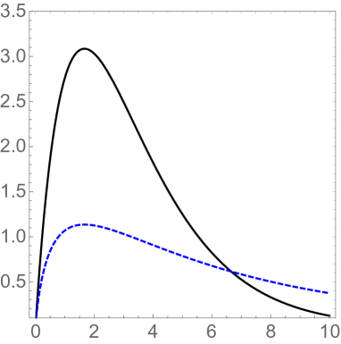
Figure 2: The ratio of the nonperturbative-to-perturbative 4-fermion effective vertex (4), with a Gaussian form factor (solid) and exponential form factor (dashed), versus the momentum transfer squared $Q^{2}\,({\rm GeV}^{2})$.

Thus, on a qualitative level one may think that the puzzling large value of the form factors at intermediate $Q$ can perhaps be understood, by adding to the perturbative diagram Fig.1(a) the nonperturbative diagram (b), with the NJL effective quark scattering of appropriate magnitude.

However, it is impossible to do it consistently. The electromagnetic, scalar or gravitational vertex (indicated by stars in this figure) may occur well $inside$ the cutoff region (indicated by a blue circle, diagram (c)) with strong nonperturbative fields, and the hypothetical nature of the local NJL interaction provides no obvious clues on how to handle propagation in it. For the minimal vector insertion, one may argue for gauge invariance to compensate for the lack-thereof in the presence of a non-local 4- or 6-quark interaction Plant and Birse (1998), but this contraint does not ensure quantum U_A(1) explicit breaking (see below), and does not extend consistently to the scalar, gravitational and more general vertices. So, one needs a more microscopic approach, providing a consistent description of quark propagation in the nonperturbative backgrounds.

I.3 Brief introduction to instanton effects

So far we focused on the (historically first) nonperturbative approach to physics of chiral symmetry breaking, namely the NJL model. With the advent of QCD in 1970^′s, this hypothetical interaction between quarks obtained more fundamental explanation which came from the understanding of gauge topology, Chern-Simons number and topological tunneling events, semiclassically described by $instantons$ Belavin et al. (1975). As discovered by t’Hooft ’t Hooft (1976), instantons indeed generate 4- and 6-fermion effective interactions of quarks. Those qualitatively differ from the NJL operator in the fact that they explicitly violate U${}_{A}(1)$ chiral symmetry, see below. By the end of 1970’s most ingredients of the instanton theory – fermionic zero modes and the propagators in the instanton field we will be using – were constructed Gross et al. (1981).

In 1980’s the main question then was whether those instanton-induced inter-quark forces are strong enough to generate chiral symmetry breaking. $Assuming$ it is so, one of us Shuryak (1982a) developed the so called instanton liquid model (ILM), using as inputs the values of the quark and gluon condensates. It assumes that the instanton ensemble have the following parameters

$$n_{I+\bar{I}}\approx 1\,{\rm fm}^{-4},\,\,\,\,\,\rho\sim 1/3\,{\rm fm}\sim 1/(0.6\,{\rm GeV})$$ (5)

for the instanton plus anti-instanton density and size, respectively. Their combination known as the diluteness parameter of the instanton ensemble is defined by

$$\kappa\equiv\pi^{2}\rho^{4}n_{I+\bar{I}}$$ (6)

These two parameters of the ILM correlates well with the parameters of the NJL model, in particular the size $\rho$ corresponds to the inverse UV cutoff. Years later, these parameters were confirmed, both by lattice studies and numerical simulation of the Interacting Instanton Liquid Model of the ensemble, for a review see Schäfer and Shuryak (1998).

The prevailing picture of the nonperturbative fields populating the QCD vacuum in 1970’s – reflected in the wide use of the OPE in the QCD sum rule framework – was a near-homogeneous vacuum fields, with characteristic momenta

$$p\sim\Lambda_{QCD}\sim 1/fm$$

The ILM had drastically changed the picture, emphasizing instead the role of the small-size instantons with relatively strong fields. For a qualitative estimate, let us mention the color summed field strength of these fields inside the instantons

$$\big{(}G^{a}_{\mu\nu}(x)\big{)}^{2}={192\rho^{4}\over(x^{2}+\rho^{2})^{4}}$$ (7)

Its magnitude at the center of a typical instanton with $\rho=1/3\,fm$ is large

$$\sqrt{\big{(}G^{a}_{\mu\nu}(0)\big{)}^{2}}=\sqrt{192}/\rho^{2}\approx 5\,{\rm GeV}^{2}$$

As we will show below, the averaging over the instanton size distribution of the induced interactions in the hard block, causes a shift towards smaller instanton sizes and stronger fields, with typically $\rho=1/6\,fm$ and $G\sim 20\,{\rm GeV}^{2}$. Such fields are by no means small compared to the the scale of the momentum transfer between quarks in the semi-hard domain under consideration. (Note also, that it is larger than the charm quark mass $m_{c}^{2}\approx 2\,{\rm GeV}^{2}$. At the end of the paper we will speculate that our light-meson results can be extrapolated in quark mass, to the strange and perhaps even charm sectors.)

Instanton fields were incorporated directly into many physical effects. The simplest are the heavy quark potentials Callan et al. (1978) and high energy scattering Shuryak and Zahed (2000), in which quark trajectories can be described by straight lines. Many more applications follow from t’Hooft effective Lagrangian ’t Hooft (1976), following from zero modes of the Dirac equation in the instanton background field, as briefly recalled in Appendix C. It is important to note that the existence of zero modes is a consequence of topological theorems, and cannot be changed by any smooth deformation of the instanton field.

The multi-quark effective Lagrangian for two quark flavors ($N_{f}=2$) consists of certain 4-quark operators. Like the NJL interaction, they preserve SU(N${}_{f})$ chiral symmetry, but $unlike$ the NJL interaction, they explicitly violate the U${}_{A}(1)$ chiral symmetry. While in “mesonic” notations, with $\sigma\equiv(\bar{q}q)$, $\vec{\pi}\equiv(\bar{q}i\gamma_{5}\vec{\tau}q)$, $\eta\equiv(\bar{q}i\gamma_{5}q)$, $\vec{\delta}\equiv(\bar{q}\vec{\tau}q)$, the NJL Lagrangian has the structure

$$L_{\rm NJL}\sim(\vec{\pi}^{2}+\sigma^{2})$$ (8)

the instanton-induced one has the structure ($N_{f}=2$)

$$L_{\rm tHooft}\sim(\vec{\pi}^{2}+\sigma^{2}-\vec{\delta}^{2}-\eta^{2})$$ (9)

It is the minus sign of the last two terms which indicates the explicit breaking of $U_{A}(1)$. Therefore in the $\eta$ channel (called $\eta^{\prime}$ for three flavors and in PDG meson tables) the interaction is not attractive but repulsive, making it heavy. In passing, we also note that the light-front wave function of the $\eta^{\prime}$ was recently calculated in Shuryak (2019), see Fig.12, and it is drastically different from that of the pions.)

With the original ILM parameters, the diluteness parameter is $\kappa\sim 1/10$, and multiple lattice studies using “deep cooling” towards the action minima have reproduced this value. This conclusion however was put in doubt by some more recent studies, which studied the dependence on the cooling time by extrapolating to its zero value time (that is, to the quantum vacuum itself). This dependence is related to instanton-antiinstanton annihilation processes during cooling. As a result, they suggested a larger value for $\kappa$.

In particular, lattice-based study Athenodorou et al. (2018) focused on the instanton contribution to 3- and 4-point Green functions in the full quantum vacuum and with cooling. Their original motivation was to extract the gluon coupling $\alpha_{s}(k)$, so the observable on which this work was focused is the the ratio of the 3-point to 2-point Green function (in configurations transformed to Landau gauge)

$$\alpha_{MOM}(k)={k^{6}\over 4\pi}{\langle G^{(3)}(k^{2})\rangle^{2}\over\langle G^{(2)}(k^{2})\rangle^{3}}$$ (10)

In the “uncooled” quantum vacuum (with gluons) the effective coupling starts running downward at large $k>1\,{\rm GeV}$, as required by asymptotic freedom. However at low $k\rightarrow 0$, one finds a persisting positive power of $k$, with a slope that matches exactly the one following from an instanton ensemble Boucaud et al. (2003)

$$\alpha_{MOM}(k)\rightarrow\frac{k^{4}}{18\pi n}$$ (11)

Furthermore, after cooling for different cooling time $\tau$, it was observed that the same power spreads to all momenta, even for $k>1\,{\rm GeV}$. This corresponds to the expectation that cooling eliminates perturbative gluons (the plain waves) but preserves (certain time-dependent fraction) of instantons.

Here, we will not cover the details of this analysis, but rather mention their main conclusion: the total instanton density (extrapolated to $zero$ cooling time) is $n\sim 10\,{\rm fm}^{-4}$, an order of magnitude larger than in the original ILM. In order words, this analysis suggests that the vacuum instanton diluteness parameter (6) is actually not small, but rather large $\kappa\sim 1$. This conclusion does not in fact contradict our understanding of the underlying of chiral symmetry breaking and the parameters of the ILM, since this large density includes close $I\bar{I}$ pairs, with zero topological charge. These molecules have a small impact on chiral symmetry breaking and related observables, and therefore were not included in the ILM. However, their internal gauge fields are very strong, and should affect nonperturbative quark scattering of the type we discuss in this paper.

II Results

In this paper we consider a larger set of form factors than it is usually done in the available literature. In particular, we discuss the pseudoscalar, vector and scalar mesons, and calculate the vector, scalar, graviton and dilaton form factors.

We also include in the distribution functions several possible Dirac/chiral structures allowed by parity. We calculate the contributions to the hard block corresponding to all four diagrams of Fig.1. Specifically, those are: (a) the perturbative one-gluon exchange; (b) the Born- style contribution of the instanton gauge field; (c) the contribution of the nonzero mode quark propagators in the instanton background; (d) the contribution of the instanton zero modes to the propagators, or t’Hooft effective 4-fermion quark interaction.

There are many technical details about these contributions, the relative values of the various parameters, etc., all of which are relegated to subsequent sections. Therefore, we decided to present the final results first, with the step-by-step derivation to be given later in the paper. Here we do not discuss the subleading contributions, the uncertainties of all parameters involved, etc. For that one has to read the paper in full. Also, the discussion of the various (light-front) wave functions (distributions), will be discussed in section V. In order to avoid too many plots, we selected a single “reasonable” example for the light-front distributions of the pion and rho mesons. For the former is is just a “flat” distribution, $\phi_{\pi}(x)=1$, and for the latter we use a simple parametrization

$$\varphi_{\rho}(\xi)\sim{\rm exp}\bigg{(}-{0.7\over 1-\xi^{2}}\bigg{)}$$ (12)

with $\xi=x-\bar{x}$, the difference between the quark and antiquark momentum fractions.

We discuss four types of elastic mesonic form factors: (a) the $vector$ ones, associated with hard scattering of a photon; (b) the $scalar$ ones, associated with scattering via a Higgs boson exchange. (Of course, those are not in practice doable, but scalar form factors were calculated numerically via lattice gauge theory simulations); (c-d) the $gravitational$ ones, associated with scattering via a graviton or dilaton exchange. In this section we report results for three contributions to each of them, of diagrams (a,c,d). Plots are provided only for the pseudoscalar and vector mesons, and only for the vector and scalar formf actors. For other cases we present the expressions for the scattering amplitudes.

II.1 Vector form factors of the pseudoscalar mesons

We will keep the notations of the contributions as explained in Fig.1. For example, the (photon-induced) vector scattering amplitude on the pion, with perturbative one-gluon exchange will be referred to as $V^{\pi}_{a}$, which is

$$V^{\pi}_{a}(Q^{2})=\epsilon_{\mu}(q)(p^{\mu}+p^{\prime\mu})\,(e_{u}+e_{\overline{d}})\,\bigg{[}\bigg{(}\frac{2C_{F}\pi\alpha_{s}f_{\pi}^{2}}{N_{c}Q^{2}}\bigg{)}$$

$$\times\int dx_{1}dx_{2}\bigg{(}{1\over\bar{x}_{1}\bar{x}_{2}+m_{\rm gluon}^{2}/Q^{2}}\bigg{)}\bigg{(}\varphi_{\pi}(x_{1})\varphi_{\pi}(x_{2})$$

$$+2{\chi_{\pi}^{2}\over Q^{2}}\bigg{(}\varphi_{\pi}^{P}(x_{1})\varphi^{P}_{\pi}(x_{2})\bigg{(}{1\over\bar{x}_{2}+E_{\perp}^{2}/Q^{2}}-1\bigg{)}+\frac{1}{6}\varphi_{\pi}^{P}(x_{1})\varphi^{\prime\,T}_{\pi}(x_{2})\bigg{(}{1\over\bar{x}_{2}+E_{\perp}^{2}/Q^{2}}+1\bigg{)}\bigg{)}\bigg{)}\bigg{]}$$

Here we show explicitly the electromagnetic charges $e_{u}=2/3,e_{\overline{d}}=1/3$, although of course the total charge of a positive pion is $e_{u}+e_{\overline{d}}=1$. The color matrices give the factor $C_{F}=(N_{c}^{2}-1)/2N_{c}=4/3$ with $N_{c}=3$ number of colors. The large spacelike photon momentum is $q^{\mu}$ and $q_{\mu}q^{\mu}=-Q^{2}<0$. The photon polarization vector is $\epsilon_{\mu}(q)$, with $\epsilon_{\mu}q^{\mu}=0$. The momenta of the initial and final mesons are called $p$ and $p^{\prime}$. The pion decay constant is $f_{\pi}\approx 133\,{\rm MeV}$, it characterizes the wave function at the origin in the transverse plane, $r_{\perp}=0$. For the pion distribution we use the expression (V.3) which includes not only the chirally diagonal part of the distribution $\varphi_{\pi}(x)$ but also the chirally non-diagonal ones, such as $\varphi_{\pi}^{P}(x)$. The DA’s depend only on one longitudinal momentum fraction $x$, which correspond to the 2-body sector of the full wave function. The regulators of the divergent integrals by extra terms in the denominators are discussed in section III.2, where the relative magnitude of both chiral contributions are compared. Here the bar indicates that the momentum fractions are those of antiquarks, $\bar{x}_{i}\equiv 1-x_{i}$. In terms of the asymmetry parameters, these variables read as $x_{i}=(1+\xi_{i})/2,\bar{x}_{i}=(1-\xi_{i})/2$. The regulators are the gluon mass and quark “transverse energy”.

Note that the last two terms $\sim\chi_{\pi}^{2}/Q^{2}$ are kept because $\chi_{\pi}$ is large, unlike the masses and transverse momenta squared of quarks which are ignored. We note further that the sum of them is shown in the summary plot in Fig. 3.

The contribution we call the Born-like instanton contribution $V_{b}^{\pi}$ has the same Dirac traces and, as explained in section III.7, and is obtained by substituting in $V_{a}^{\pi}$ the Fourier transforms of the instanton gauge field (59) instead of the gluon propagator, with

$$\pi\alpha_{s}(Q/2)\rightarrow\kappa\left<\mathbb{G}^{2}(Q\rho\sqrt{\overline{x}_{1}\overline{x}_{2}})\right>$$ (14)

and is therefore

$$V^{\pi}_{b}(Q^{2})=\epsilon_{\mu}(q)(p^{\mu}+p^{\prime\mu})\,(e_{u}+e_{\overline{d}})\,\bigg{[}\bigg{(}\frac{2C_{F}\kappa f_{\pi}^{2}}{N_{c}Q^{2}}\bigg{)}$$

$$\times\int dx_{1}dx_{2}\,\left<\mathbb{G}^{2}(Q\rho\sqrt{\overline{x}_{1}\overline{x}_{2}})\right>\bigg{(}{1\over\bar{x}_{1}\bar{x}_{2}+m_{\rm gluon}^{2}/Q^{2}}\bigg{)}\bigg{(}\varphi_{\pi}(x_{1})\varphi_{\pi}(x_{2})$$

$$+2{\chi_{\pi}^{2}\over Q^{2}}\bigg{(}\varphi_{\pi}^{P}(x_{1})\varphi^{P}_{\pi}(x_{2})\bigg{(}{1\over\bar{x}_{2}+E_{\perp}^{2}/Q^{2}}-1\bigg{)}+\frac{1}{6}\varphi_{\pi}^{P}(x_{1})\varphi^{\prime}_{T}(x_{2})\bigg{(}{1\over\bar{x}_{2}+E_{\perp}^{2}/Q^{2}}+1\bigg{)}\bigg{)}\bigg{)}\bigg{]}$$

The instanton induced form factor $\mathbb{G}$ is given in (59). The angular brackets indicate averaging over the instanton size.

The contribution $V_{c}^{\pi}$, from three $non$-zero mode propagators, are discussed in section IV.1, it leads to the following result

$$V_{c}^{\pi}= \epsilon_{\mu}(q)(p^{\mu}+p^{\prime\mu})\,(e_{u}+e_{\overline{d}})\,\bigg{[}{\kappa\pi^{2}f_{\pi}^{2}\chi_{\pi}^{2}\over N_{c}M_{Q}^{2}}\langle\rho^{2}{\mathbb{G}}_{V}(Q\rho)\rangle$$ (16)

$$\times\int dx_{1}dx_{2}\overline{x}_{1}\bigg{(}\varphi_{\pi}^{P}(x_{1})\varphi_{\pi}^{P}(x_{2})-\frac{1}{36}\varphi_{\pi}^{{}^{\prime}T}(x_{1})\varphi_{\pi}^{{}^{\prime}T}(x_{2})\bigg{)}\bigg{]}$$

The function $\mathbb{G}_{V}$ is given in (75). Again, the angular brackets indicate that it is averaged over the instanton size distribution, as explained in section IV.10. Note that the partonic integrand involves a single momentum fraction $\bar{x}_{1}$ (or $\bar{x}_{2}$ in the symmetric term not shown). The other integral is simply over the function itself. For all of them except $\varphi_{\pi}^{{}^{\prime}T}$ it is the normalization integral equal to 1. Yet for this one it is an integral of the derivative, and therefore it vanishes due to the quark-antiquark symmetry $x\leftrightarrow\bar{x}$

$$\int_{0}^{1}\varphi_{\pi}^{{}^{\prime}T}(x)dx=\varphi_{\pi}^{T}(1)-\varphi_{\pi}^{T}(0)\rightarrow 0$$ (17)

so the last term in (16) does not actually contribute to the form factor.

The contribution of the mixed zero mode and non-zero mode (^′t Hooft vertex) derived in section IV.5, to the pion vector form factor is

$$V_{d}^{\pi}=-\epsilon_{\mu}(q)(p^{\mu}+p^{\prime\mu})\,(e_{u}+e_{\overline{d}})\,$$ (18)

$$\times\bigg{[}\bigg{(}\frac{1}{N_{c}^{2}(N_{c}+1)}\bigg{)}\frac{4\kappa\pi^{2}f_{\pi}^{2}\chi_{\pi}^{2}}{3M_{Q}^{2}}\left<\rho^{2}\frac{K_{1}(Q\rho)}{Q\rho}\right>\int dx_{1}dx_{2}\varphi_{\pi}^{P}(x_{1})\varphi_{\pi}^{{}^{\prime}T}(x_{2})\bigg{]}$$

As we noted in (17), this contribution vanishes after the $x$ integration is carried.

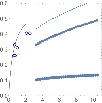
Figure 3: The vector form factors of the pion times the squared momentum transfer, $Q^{2}F_{\pi}(Q^{2})\,\,({\rm GeV}^{2})$ versus $Q^{2}({\rm GeV}^{2})$. The closed discs show the total perturbative contribution. The squares correspond to the instanton contribution from the non-zero mode propagators $S_{NZ}$. The dotted line above is their sum. The solid line is the usual dipole fit with the rho meson mass, and the open points are from the experimental measurements. We do not show the multiple data points at smaller $Q^{2}$, where there is good agreement with the dipole formula.

The summary plot of the pion vector form factor is shown in Fig. 3, taking all three DA’s as flat distributions $\varphi_{\pi}(x)=\varphi^{P}_{\pi}(x)=1$ and $\varphi^{{}^{\prime}T}_{\pi}=0$. This selection is motivated by our view that the flat distributions represent an upper bound on the DA, with the asymptotic form providing a lower bound.

The perturbative contributions $V_{a}^{\pi}$ (closed circles) is the sum of all chiral structures of the pion density matrices. The corresponding integrals for each of them separately are shown in Fig.7, from which it is seen that the chiral-nondiagonal term is about twice larger than the chiral-diagonal one in the range of momenta considered. This feature was anticipated already in Geshkenbein and Terentev (1982).

The instanton Born-style contributions to $V_{b}^{\pi}$ is relatively close to $V_{a}^{\pi}$ if the instanton diluteness parameter is $\kappa=1$. (For a discussion of its value see the end of section I.3.) To avoid any misunderstanding, we note that the $V^{\pi}_{b}$ conribution does $not$ really constitute a consistent account for the instanton effects, as are $V^{\pi}_{c},\,\,V^{\pi}_{d}$, and therefore is $not$ shown in the summary plot.

The instanton-induced contribution $V_{c}^{\pi}$ (squares) at $\kappa=1$ is comparable to the perturbative $V_{a}^{\pi}$ in magnitude, but has a different dependence on $Q^{2}$. The instanton form factor is of course a decreasing function of momentum transfer, but on the plot it is multiplied by an extra $Q^{2}$ and is therefore slowly increasing.

Taken together (dotted line at the top) they account for the pion form factor for the corresponding values of $Q^{2}$, reasonably well joining the experimental data at the lower end. We stress that no parameters were fitted for this to happen. Our main focus is still a comparison between all plots, with the same set of parameters.

II.2 Scalar form factors of the pion

One may think of a point-like scalar quantum, hitting one of the quarks with momentum transfer $q^{\mu}$ to be the Higgs boson. If so, the corresponding couplings are Yukawa couplings $\lambda_{q},q=u,d,...$ of the standard model. However, these couplings are unimportant for the form factors. (E.g. lattice groups use for convenience $\lambda_{u}=1,\lambda_{d}=0$). The corresponding amplitude of the elastic scattering on a pion, with a perturbative one-gluon exchange between quarks, leads to the following scattering amplitude

$$S_{a}^{\pi}=-(\lambda_{u}+\lambda_{d})M_{Q} \bigg{[}\bigg{(}\frac{2\pi C_{F}\alpha_{s}f_{\pi}^{2}\chi_{\pi}}{N_{c}Q^{2}M_{Q}}\bigg{)}\,\int_{0}^{1}{dx_{1}dx_{2}\over\overline{x}_{1}\overline{x}_{2}+m_{gluon}^{2}/Q^{2}}$$ (19)

$$\times\bigg{(}\varphi_{\pi}(x_{1})\varphi_{\pi}^{P}(x_{2})\bigg{(}1+{2\over\overline{x}_{2}+E_{\perp}^{2}/Q^{2}}\bigg{)}+{1\over 6}\varphi_{\pi}(x_{1})\varphi_{\pi}^{T\prime}(x_{2})\bigg{)}\bigg{]}$$

Note first that we included outside the square bracket the quark constituent mass $M_{Q}$, which is balanced by the same constituent mass in the denominator. We did it to facilitate the comparison with the instanton-induced expressions to follow.

In the previous section, on the vector form factor, it was obvious that the factors with charges and momenta in the amplitude do not belong to form factors, as they are also present in the forward scattering at $Q=0$. The situation with the scalar formf actors is a bit different. The forward scattering amplitude on a hadron $h$ is proportional to

$$\sum_{q}\lambda_{q}\langle h|\bar{q}q|h\rangle=-\sum_{q}\lambda_{q}{\partial M^{2}_{h}\over\partial m_{q}}$$ (20)

thanks to the Feynman-Hellman theorem. The derivative appearing here is known for the pion from the Gell-Mann-Oaks-Renner relation, and for most hadrons from lattice chiral extrapolations.

In the scalar plots to follow, we will the show square brackets in the amplitudes times $Q^{2}$ without the factors in front, as we did for the vector cases. Indeed, our main focus is on the relative magnitude of different contributions. However the reader should be cautioned that the true scalar formf actor $F_{S}(Q^{2})$ requires multiplication by an additional factor

$$K_{S}={\sum_{q}\lambda_{q}\partial M^{2}_{h}/\partial m_{q}\over M_{Q}\sum_{q}\lambda_{q}}$$ (21)

to enforce the standard form factor normalization $F_{S}(Q=0)=1$.

An additional contribution proportional to the quark mass $M_{Q}$, instead of $\chi_{\pi}$, is explicitly given in (45), but, being subleading, it is not mentioned here.

Note also that the scalar amplitudes have negative overall sign, which really does not matter as the couplings $\lambda_{q}$ are arbitrary. This sign of course does not affect the contribution to the form factor as captured by the square bracket. The Born-like instanton contribution to the scalar pion scattering, $S_{b}^{\pi}$, is obtained by the same substitution (14) to $S_{a}^{\pi}$ and is therefore not shown here.

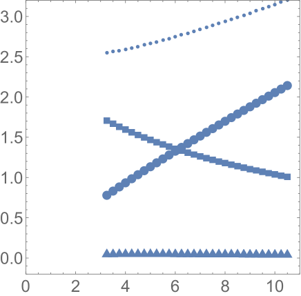
Figure 4: We show the square bracket in the scalar scattering amplitudes of the pion as in (19) etc, times the momentum transfer squared $({\rm GeV}^{2})$, versus $Q^{2},({\rm GeV}^{2})$. As in the previous plot, the black closed disks correspond to the one-gluon exchange contribution, the black squares to the instanton contribution from three non-zero mode propagators $S_{NZ}$, the black triangles correspond to the zero-mode terms $S_{Z}$ in two propagators. The dotted line above is their sum. (We recall that the full normalized scalar form factor is obtained by multiplying these results by the extra factor (21).)

The contribution of the instanton-induced diagram (c) (with three nonzero mode propagators) is

$$S_{c}^{\pi}(Q^{2})= -(\lambda_{u}+\lambda_{\overline{d}})\,M_{Q}\,\bigg{[}\bigg{(}\frac{\kappa\pi^{2}\chi_{\pi}f_{\pi}^{2}}{N_{c}M_{Q}^{3}}\bigg{)}\,\left<(Q\rho)^{2}\mathbb{G}_{S}(Q\rho)\right>\,$$ (22)

$$\times\int_{0}^{1}dx_{1}dx_{2}\,\bar{x}_{2}\varphi_{\pi}(x_{1})\bigg{(}\varphi_{\pi}^{P}(x_{2})-\frac{1}{6}\varphi_{\pi}^{T\prime}(x_{2})\bigg{)}\bigg{]}$$

Unlike the vector form factor $V_{c}^{\pi}$ (16), the scalar form factor here involves the form factor ${\mathbb{G}}_{S}$ in (77), which is part of ${\mathbb{G}}_{V}$.

The contribution from the mixed zero modes and non-zero modes or ’t Hooft vertex is

$$S_{d}^{\pi}(Q^{2})= -(\lambda_{u}+\lambda_{\overline{d}})\,M_{Q}\,\bigg{[}\bigg{(}\frac{1}{N_{c}^{2}(N_{c}+1)}\bigg{)}\bigg{(}\frac{\kappa\pi^{2}f_{\pi}^{2}\chi_{\pi}}{M_{Q}^{3}}\bigg{)}\,\left<Q\rho K_{1}(Q\rho)\right>$$

$$\times\,\int_{0}^{1}dx_{1}dx_{2}\,\bigg{(}x_{1}\varphi_{\pi}(x_{2})\bigg{(}\varphi_{\pi}^{P}(x_{1})+\frac{1}{6}\varphi_{\pi}^{T\prime}(x_{1})\bigg{)}+x_{2}\varphi_{\pi}(x_{1})\bigg{(}\varphi_{\pi}^{P}(x_{2})+\frac{1}{6}\varphi_{\pi}^{T\prime}(x_{2})\bigg{)}\bigg{)}\bigg{]}$$

The perturbative and instanton contributions to the scalar form factor of the pion (with flat DA’s) are shown in Fig.4 versus $Q^{2}$. Again, one finds them to be comparable in magnitude but quite different in their $Q$ dependence. Moreover, their sum is roughly independent of $Q^{2}$.

II.3 Form factors of transversely polarized vector mesons

The transversely polarized rho meson form factors are both electric and magnetic (see below). For simplicity, we quote here the contribution to the electric or charge form factor by choosing the transverse polarization $\epsilon_{T}(p,p^{\prime})$ of the $\rho$ with momentum $p,p^{\prime}$ to be also transverse to $q$, or $\epsilon_{T}(p,p^{\prime})\cdot q=0$.

The perturbative contribution (a) for the transversely polarized rho vector form factor is formally subleading (containing an extra factor of $m_{\rho}^{2}/Q^{2}$), like the $\chi_{\pi}^{2}/Q^{2}$ contribution in the second term of $V_{a}^{\pi}$, and is found to be

$$V^{\rho}_{a}(Q^{2})= \epsilon_{\mu}(q)(p^{\mu}+p^{\prime\mu})\,(e_{u}+e_{\overline{d}})\,(-\epsilon^{\prime*}_{T}\cdot\epsilon_{T})\,\bigg{(}\frac{2\pi C_{F}\alpha_{s}f_{\rho}^{2}m_{\rho}^{2}}{N_{c}Q^{4}}\bigg{)}\int_{0}^{1}{dx_{1}dx_{2}\over\bar{x}_{1}\bar{x}_{2}+m_{\rm gluon}^{2}/Q^{2}}$$ (24)

$$\times\bigg{[}\bigg{(}\varphi_{\rho}(x_{1})\varphi_{\rho}(x_{2})-\frac{1}{16}\varphi^{A\prime}_{\rho}(x_{1})\varphi^{A\prime}_{\rho}(x_{2})\bigg{)}\bigg{(}{1\over\bar{x}_{1}+E_{\perp}^{2}/Q^{2}}+{1\over\bar{x}_{2}+E_{\perp}^{2}/Q^{2}}-2\bigg{)}$$

$$+{1\over 2}\varphi^{A\prime}_{\rho}(x_{1})\varphi_{\rho}(x_{2})\bigg{(}{1\over\bar{x}_{1}+E_{\perp}^{2}/Q^{2}}-{1\over\bar{x}_{2}+E_{\perp}^{2}/Q^{2}}\bigg{)}\bigg{]}$$

Note that the minus sign in the product of polarization vectors in fact means that this contribution is $positive$, since $\epsilon^{*}_{T}\cdot\epsilon_{T}^{\prime}<0$ in the Minkowski metric used here. The Born-like instanton contribution to the rho vector form factor $V_{b}^{\rho}$ is also given by the substitution (14) to $V_{a}^{\rho}$, and will not be given.

The one-gluon exchange to the scalar form factor of the transverse rho meson is

$$S^{\rho}_{a}(Q^{2})=-(\lambda_{u}+\lambda_{\overline{d}})\,M_{Q}\,(-\epsilon^{\prime*}_{T}\cdot\epsilon_{T})\bigg{[}\bigg{(}\frac{\pi C_{F}\alpha_{s}}{N_{c}}\,\frac{m_{\rho}f_{\rho}f^{T}_{\rho}}{M_{Q}Q^{2}}\bigg{)}$$

$$\times\int{dx_{1}dx_{2}\over\overline{x}_{1}\overline{x}_{2}+m^{2}_{\rm gluon}/Q^{2}}\bigg{(}\frac{\varphi^{T}_{\rho}(x_{1})(\varphi_{\rho}(x_{2})-\varphi^{A\prime}_{\rho}(x_{2})/4)}{\overline{x}_{1}+E_{\perp}^{2}/Q^{2}}+\frac{(\varphi_{\rho}(x_{1})-\varphi_{\rho}^{A\prime}(x_{1})/4)\varphi^{T}_{\rho}(x_{2})}{\overline{x}_{2}+E_{\perp}^{2}/Q^{2}}\bigg{)}\bigg{]}$$

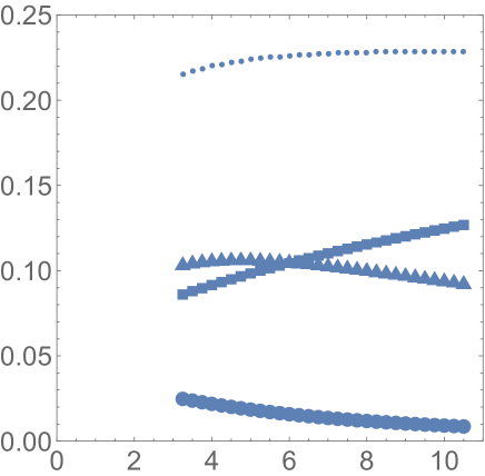
Figure 5: The vector form factors of the transversely polarized rho meson, times the momentum transfer squared , $Q^{2}F^{S}_{\pi}(Q^{2})\,\,({\rm GeV}^{2})$ versus $Q^{2},({\rm GeV}^{2})$. The black closed points show the perturbative contribution, the black triangles correspond to the instanton zero mode (’t Hooft vertex) contribution, and the squares are the contribution of the non-zero mode propagators $S_{NZ}$. The dotted line above is their sum.

The contribution of the the mixed zero mode and non-zero mode to the transverse rho meson vector form factor is

$$V_{c}^{\rho}(Q^{2})= \epsilon_{\mu}(q)(p^{\mu}+p^{\prime\mu})\,(e_{u}+e_{\overline{d}})\,(-\epsilon^{\prime*}_{T}\cdot\epsilon_{T})\bigg{[}{\kappa\pi^{2}f_{\rho}^{2}m_{\rho}^{2}\over N_{c}M_{Q}^{2}}\,\left<\rho^{2}\mathbb{G}_{V}(Q\rho)\right>\,$$ (26)

$$\times\int_{0}^{1}dx_{1}dx_{2}\,\bar{x}_{1}\bigg{(}\varphi_{\rho}(x_{1})-\frac{\varphi_{\rho}^{A\prime}(x_{1})}{4}\bigg{)}\bigg{(}\varphi_{\rho}(x_{2})+\frac{\varphi_{\rho}^{A\prime}(x_{2})}{4}\bigg{)}\bigg{]}$$

The contribution of the mixed zero mode and non-zero mode to the rho meson scalar form factor is

$$S_{c}^{\rho}(Q^{2})=-(\lambda_{u}+\lambda_{\overline{d}})\,M_{Q}\,(-\epsilon^{\prime*}_{T}\cdot\epsilon_{T})\,\bigg{[}\bigg{(}\frac{\kappa\pi^{2}f_{\rho}f^{T2}_{\rho}m_{\rho}}{4N_{c}M_{Q}^{4}}\bigg{)}\,\left<(Q\rho)^{2}{\mathbb{G}}_{S}(Q\rho)\right>$$

$$\times\int dx_{1}dx_{2}\bigg{(}\bar{x}_{1}\bigg{(}\varphi_{\rho}(x_{1})-\frac{\varphi^{A\prime}_{\rho}(x_{1})}{4}\bigg{)}\varphi^{T}_{\rho}(x_{2})+\bar{x}_{2}\bigg{(}\varphi_{\rho}(x_{2})-\frac{\varphi^{A\prime}_{\rho}(x_{2})}{4}\bigg{)}\varphi^{T}_{\rho}(x_{1})\bigg{)}\bigg{]}$$ (27)

The contribution of the ’t Hooft vertex to the vector form factor of the transversely polarized rho is detailed in (114) with the result

$$V_{d}^{\rho}(Q^{2})=-(e_{u}+e_{\overline{d}})\bigg{(}\epsilon_{\mu}(q)(p^{\mu}+p^{\prime\mu})\,(\epsilon^{\prime*}_{T}\cdot\epsilon_{T})\bigg{)}\,\bigg{[}\left<Q\rho\,K_{1}(Q\rho)\right>\,\bigg{(}\frac{2\kappa\pi^{2}}{N_{c}^{2}(N_{c}+1)}\frac{{f^{T2}_{\rho}}}{M^{2}_{Q}}\bigg{)}\bigg{]}$$ (28)

The contribution of the mixed non-zro mode and zero-mode contribution (’t Hooft vertex) to the scalar form factor of the transversely polarized rho is

$$S_{d}^{\rho}(Q^{2})= +(\lambda_{u}+\lambda_{\overline{d}})\,M_{Q}\,(-\epsilon^{\prime*}_{T}\cdot\epsilon_{T})\bigg{[}\bigg{(}\frac{1}{N_{c}^{2}(N_{c}+1)}\bigg{)}\bigg{(}\frac{\kappa\pi^{2}f_{\rho}f_{\rho}^{T}m_{\rho}}{M_{Q}^{3}}\bigg{)}\,\left<Q\rho K_{1}(Q\rho)\right>$$

$$\times\,\int_{0}^{1}dx_{1}dx_{2}\,\bigg{(}x_{1}\varphi^{T}(x_{2})\bigg{(}\varphi_{\rho}(x_{1})+\frac{1}{4}\varphi_{\rho}^{A\prime}(x_{1})\bigg{)}+x_{2}\varphi_{\rho}^{T}(x_{1})\bigg{(}\varphi_{\rho}(x_{2})+\frac{1}{4}\varphi_{\rho}^{A\prime}(x_{2})\bigg{)}\bigg{)}\bigg{]}$$

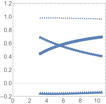
Figure 6: The square bracket quoted in the scalar scattering amplitudes of the rho given in the text, times the momentum transfer squared $Q^{2}[...]\,\,\,({\rm GeV}^{2})$ versus $Q^{2},({\rm GeV}^{2})$. The black closed points correspond to the one-gluon exchange contribution, the black squares to the instanton contribution of three non-zero mode propagators $S_{NZ}$, and the black triangles to the zero-mode terms $S_{Z}$ in two propagators. The dotted line above is their sum. (Recall that the normalized scalar form factor is obtained by multiplication by the extra factor in (21).)

Completing this section, let us summarize the lessons from these four plots: a/ the first conclusion stemming from all of them, is that the instanton effects are indeed comparable to the perturbative ones in magnitude.; b/ the second conclusion is that, while separate contributions have different $Q$-dependence, the total sums tend to be flat. While this conclusion seems to correspond to lattice data, we still need to remind the reader that the $absolute$ normalization of the instanton-induced effects (squares and triangles in the previous 4 plots) remains relatively uncertain. The value $\kappa=1$ is motivated (as for the DAs) to represent the “maximal but reasonable” value. The quark mass used $M_{Q}=0.4\,{\rm GeV}$ may be strongly modified in the denominators. With better knowledge of the gauge topology and DAs, these curves may be modified.

We end this section by noting that the hard block is not sensitive to the current quark mass $m_{q}$, as it was assumed that $Q^{2}\gg m_{q}^{2}$. Therefore, going from the pion to $\eta_{s}$ and perhaps even $\eta_{c}$ (in the appropriate kinematic range) one only needs to change the wave functions and the decay constant $f_{\pi}\rightarrow f_{\eta s}$. We will discuss the comparison to lattice data in section VI.2.

II.4 Form factors of the scalar meson $a_{0}^{+}$

The form factors of the scalar meson $a_{0}^{+}$ results from the same hard blocks, but with completely different DA’s. The vector form factor of the $a_{0}^{+}$ meson is

$$V^{a0}_{a}(Q^{2})=\epsilon_{\mu}(q)(p^{\mu}+p^{\prime\mu})\,(e_{u}+e_{\overline{d}})\,\bigg{[}\bigg{(}\frac{2C_{F}\pi\alpha_{s}f_{a0}^{2}}{N_{c}Q^{2}}\bigg{)}\int{dx_{1}dx_{2}\over\bar{x}_{1}\bar{x}_{2}+m_{\rm gluon}^{2}/Q^{2}}\bigg{(}\varphi^{V}_{a0}(x_{1})\varphi^{V}_{a0}(x_{2})$$

$$+{2\over Q^{2}}\bigg{(}(\chi_{a0}^{S})^{2}\varphi_{a0}^{S}(x_{1})\varphi^{S}_{a0}(x_{2})\bigg{(}{1\over\bar{x}_{2}+E_{\perp}^{2}/Q^{2}}-1\bigg{)}+{\chi_{a0}^{S}\chi_{a0}^{T}\over 6}\varphi_{a0}^{S}(x_{1})\varphi_{a0}^{\prime\,T}(x_{2})\bigg{(}{1\over\bar{x}_{2}+E_{\perp}^{2}/Q^{2}}+1\bigg{)}\bigg{)}\bigg{]}$$

which is to be compared with (II.1). All constants are different than in the pion case. The repulsive character of the interaction in this channel should penalize the wavefunction at the origin, leading to smaller values for the parameters in comparison to the pion parameters.

The scalar form factor of the $a_{0}^{+}$ reads

$$S_{a}^{a_{0}}(Q^{2})=-(\lambda_{u}+\lambda_{d})\,M_{Q}\,\bigg{[}\bigg{(}\frac{2C_{F}\pi\alpha_{s}f_{a_{0}}^{2}}{N_{c}M_{Q}Q^{2}}\bigg{)}\,$$

$$\times\int_{0}^{1}{dx_{1}dx_{2}\over\overline{x}_{1}\overline{x}_{2}+m_{gluon}^{2}/Q^{2}}\bigg{(}\chi_{a_{0}}^{S}\varphi^{S}_{a_{0}}(x_{1})\varphi^{V}_{a_{0}}(x_{2})\bigg{(}1+\frac{2}{\bar{x}_{2}+E_{\perp}^{2}/Q^{2}}\bigg{)}+\chi_{a_{0}}^{T}\varphi^{V}_{a_{0}}(x_{1})\frac{\varphi_{a_{0}}^{T\prime}(x_{2})}{6}\bigg{)}\bigg{]}$$

which is structurally similar to the pion result (19).

The non-zero mode propagators contribute to the vector and scalar form factors of the $a_{0}^{+}$ as follows

$$V_{c}^{a_{0}}=\epsilon_{\mu}(q)(p^{\mu}+p^{\prime\mu})\,(e_{u}+e_{\overline{d}})\,\bigg{[}\bigg{(}{\kappa\pi^{2}f_{a_{0}}^{2}\over N_{c}M_{Q}^{2}}\bigg{)}\langle\rho^{2}{\mathbb{G}}_{V}(Q\rho)\rangle$$

$$\times\int dx_{1}dx_{2}\bigg{(}\overline{x}_{1}(\chi_{a_{0}}^{S})^{2}\varphi_{a_{0}}^{S}(x_{1})\varphi_{a_{0}}^{S}(x_{2})-(\overline{x}_{2}-\overline{x}_{1})\varphi_{a_{0}}^{S}(x_{1})\frac{\chi_{a_{0}}^{S}\chi_{a_{0}}^{T}\varphi_{a_{0}}^{T\prime}(x_{2})}{6}-\bar{x}_{1}\frac{(\chi_{a_{0}}^{T})^{2}\varphi_{a_{0}}^{T\prime}(x_{1})}{6}\frac{\varphi_{a_{0}}^{T\prime}(x_{2})}{6}\bigg{)}\bigg{]}$$

(32)

is similar to (16)

$$S_{c}^{a_{0}}(Q^{2})= -(\lambda_{u}+\lambda_{\overline{d}})\,M_{Q}\,\bigg{[}\bigg{(}\frac{\kappa\pi^{2}f_{a_{0}}^{2}}{N_{c}M_{Q}^{3}}\bigg{)}\,\left<(Q\rho)^{2}\mathbb{G}_{S}(Q\rho)\right>\bigg{]}\,$$ (33)

$$\times\int_{0}^{1}dx_{1}dx_{2}\,\bigg{[}\bar{x}_{2}\varphi^{V}_{a_{0}}(x_{1})\bigg{(}\chi_{a_{0}}^{S}\varphi^{S}_{a_{0}}(x_{2})-\frac{1}{6}\chi_{a_{0}}^{T}\varphi_{a_{0}}^{T\prime}(x_{2})\bigg{)}\bigg{]}$$

The contribution of the mixed zero mode and non-zero mode propagators (^′t Hooft vertex) to the $a_{0}^{+}$ vector form factor is

$$V_{d}^{a_{0}}(Q^{2})=\epsilon_{\mu}(q)(p^{\mu}+p^{\prime\mu})\,(e_{u}+e_{\overline{d}})\,$$

$$\times\bigg{[}\bigg{(}\frac{1}{N_{c}^{2}(N_{c}+1)}\bigg{)}\frac{4\kappa\pi^{2}f_{a_{0}}^{2}\chi_{a_{0}}^{S}\chi_{a_{0}}^{T}}{3M_{Q}^{2}}\left<\rho^{2}\frac{K_{1}(Q\rho)}{Q\rho}\right>\int dx_{1}dx_{2}\varphi_{a_{0}}^{S}(x_{1})\varphi_{a_{0}}^{T\prime}(x_{2})\bigg{]}$$ (34)

As we noted for the pion in (18), this contribution vanishes after the partonic integration is carried.

The contribution from the mixed zero modes and non-zero modes or ’t Hooft vertex to the scalar form factor of the $a_{0}^{+}$ meson is

$$S_{d}^{a_{0}}(Q^{2})= +(\lambda_{u}+\lambda_{\overline{d}})\,M_{Q}\,\bigg{[}\bigg{(}\frac{1}{N_{c}^{2}(N_{c}+1)}\bigg{)}\bigg{(}\frac{\kappa\pi^{2}f_{a_{0}}^{2}}{M_{Q}^{3}}\bigg{)}\,\int_{0}^{1}dx_{1}dx_{2}\,\left<Q\rho K_{1}(Q\rho)\right>$$

$$\times\,\bigg{(}x_{1}\varphi^{V}_{a_{0}}(x_{2})\bigg{(}\chi_{a_{0}}^{S}\varphi_{a_{0}}^{S}(x_{1})+\frac{1}{6}\chi_{a_{0}}^{T}\varphi_{a_{0}}^{T\prime}(x_{1})\bigg{)}+x_{2}\varphi^{V}_{a_{0}}(x_{1})\bigg{(}\chi_{a_{0}}^{S}\varphi_{a_{0}}^{S}(x_{2})+\frac{1}{6}\chi_{a_{0}}^{T}\varphi_{a_{0}}^{T\prime}(x_{2})\bigg{)}\bigg{)}\bigg{]}$$

We note the overall sign flip in comparison to the pion contribution in (II.2), but otherwise a similar structural result.

II.5 Graviton and dilaton form factors of the pion

The energy-momentum form factor of the pion follows follows from the replacement of the vector vertex by the symmetrized tensor vertex (III.4). The form factor decomposition is detailed in III.4 with the $00$ (graviton) and $\mu\mu$ (dilaton) perturbative contributions

$$T^{\pi}_{00a}(Q^{2})= \bigg{(}\frac{4C_{F}\pi\alpha_{s}f_{\pi}^{2}}{N_{c}}\bigg{)}\int dx_{1}dx_{2}\,\frac{1}{\bar{x}_{1}\bar{x}_{2}+m_{\rm gluon}^{2}/Q^{2}}\bigg{(}x_{1}\varphi_{\pi}(x_{1})\varphi_{\pi}(x_{2})$$

$$+\frac{2\chi_{\pi}^{2}}{Q^{2}}\bigg{(}\bigg{(}\frac{1}{\bar{x}_{1}+E_{\perp}^{2}/Q^{2}}+\bar{x}_{1}-2\bigg{)}\varphi_{\pi}^{P}(x_{1})\varphi_{\pi}^{P}(x_{2})+\bigg{(}\frac{1}{\bar{x}_{1}+E_{\perp}^{2}/Q^{2}}-\bar{x}_{1}\bigg{)}\varphi_{\pi}^{P}(x_{2})\frac{\varphi_{\pi}^{T\prime}(x_{1})}{6}\bigg{)}$$

$$T^{\pi}_{\mu\mu a}(Q^{2})= \bigg{(}\frac{4C_{F}\pi\alpha_{s}f_{\pi}^{2}}{N_{c}}\bigg{)}\int dx_{1}dx_{2}\,\frac{1}{\bar{x}_{1}\bar{x}_{2}+m_{\rm gluon}^{2}/Q^{2}}\bigg{(}\varphi_{\pi}(x_{1})\varphi_{\pi}(x_{2})$$

$$+\frac{2\chi_{\pi}^{2}}{Q^{2}}\bigg{(}\bigg{(}\frac{1}{\bar{x}_{1}+E_{\perp}^{2}/Q^{2}}-3\bigg{)}\varphi_{\pi}^{P}(x_{1})\varphi_{\pi}^{P}(x_{2})+\bigg{(}\frac{1}{\bar{x}_{1}+E_{\perp}^{2}/Q^{2}}-1\bigg{)}\varphi_{\pi}^{P}(x_{2})\frac{\varphi_{\pi}^{T\prime}(x_{1})}{6}\bigg{)}$$

The non-zero mode contribution follows the same reasoning as that for the vector contribution through the substitution (III.4), with the result

$$T^{\pi}_{00c}(Q^{2})= \bigg{(}\frac{\kappa\pi^{2}f_{\pi}^{2}\chi_{\pi}^{2}}{N_{c}M_{Q}^{2}}\bigg{)}\left<(Q\rho)\mathbb{G}_{V}(Q\rho)\right>\int dx_{1}dx_{2}\,(\bar{x}_{1}-\bar{x}_{2})$$

$$\times\bigg{(}\bar{x}_{1}\varphi_{\pi}^{P}(x_{1})\varphi_{\pi}^{P}(x_{2})+(\bar{x}_{2}-\bar{x}_{1})\varphi_{\pi}^{P}(x_{2})\frac{\varphi_{\pi}^{T\prime}(x_{1})}{6}-\bar{x}_{1}\frac{\varphi_{\pi}^{T\prime}(x_{1})}{6}\frac{\varphi_{\pi}^{T\prime}(x_{2})}{6}\bigg{)}$$

$$T^{\pi}_{\mu\mu c}(Q^{2})= \bigg{(}\frac{2\kappa\pi^{2}f_{\pi}^{2}\chi_{\pi}^{2}}{N_{c}M_{Q}^{2}}\bigg{)}\left<(Q\rho)\mathbb{G}_{V}(Q\rho)\right>\int dx_{1}dx_{2}\,\bar{x}_{1}x_{2}$$ (37)

$$\times\bigg{(}\varphi_{\pi}^{P}(x_{1})\varphi_{\pi}^{P}(x_{2})-\varphi_{\pi}^{P}(x_{2})\frac{\varphi_{\pi}^{T\prime}(x_{1})}{6}-\frac{\varphi_{\pi}^{T\prime}(x_{1})}{6}\frac{\varphi_{\pi}^{T\prime}(x_{2})}{6}\bigg{)}$$

The mixed-zero mode and non-zero mode contribution (83) contribute equally to $00$ and $\mu\mu$ in the Breit frame, with the result

$$T^{\pi}_{00d}(Q^{2})=T^{\pi}_{\mu\mu d}(Q^{2})=-\frac{1}{N_{c}^{2}(N_{c}+1)}\bigg{(}\frac{16\kappa\pi^{2}f_{\pi}^{2}\chi_{\pi}^{2}}{3M_{Q}^{2}}\bigg{)}\left<(Q\rho)K_{1}(Q\rho)\right>\int dx_{1}dx_{2}\,\varphi_{\pi}(x_{1})\frac{\varphi_{\pi}^{T\prime}(x_{2})}{6}$$ (38)

which is seen to vanish after $x$ integration.

III Hard block from one-gluon exchange and its possible extensions

III.1 The one-gluon exchange contributions

After we presented the results, we now turn to their derivation starting from the hard block induced by the lowest order perturbative diagram, for completeness.

The one-gluon exchange contribution to the mesonic form factor is illustrated in Fig. 1(a), where also the definition of the momenta involved is also given (see also Appendix A). Of course, Fig. 1(a) is one of four diagrams, with a photon insertion appearing on the upper line of the $u$-quark before the gluon vertex. In the Breit frame, the space-like photon carries $q=(0,0,Q,0)$, with the energy as the 4-th component. The incoming pion carries $p=(0,0,-Q/2,\sqrt{m_{\pi}^{2}+(Q/2)^{2}})$ and the outgoing pion carries ${p}^{\prime}=(0,0,+Q/2,\sqrt{m_{\pi}^{2}+(Q/2)^{2}})$. We will however ignore the pion mass $m_{\pi}$ in the energy, by approximating the latter by $Q/2$ in the hard momentum limit.

The quark momenta should not be directed strictly along the direction of the meson momentum, as they carry some nonzero transverse momenta $\vec{k}_{\perp}\neq 0$ in the wave functions. In principle, one needs to integrate over their distribution in hadrons. This brings in a question discussed e.g. in Chibisov and Zhitnitsky (1995), who pointed out that the smallness of the mean transverse momenta $\langle k_{\perp}^{2}\rangle\ll Q^{2}$ does not in general exclude the existence and importance of a wave function component with a larger $k_{\perp}^{2}\sim Q^{2}$. In particular, it can also be induced by instantons, as momenta and field strength are simply related by the equations of motion. In general, such a component, when present, would violate factorization and produce an additional contribution to the exclusive processes.

Nevertheless, in this paper we will for now ignore such contributions. The wave functions depending on $k_{\perp}$ will appear only in the integrated DA’s, times the probability to find both quarks at the same transverse location. Those are constants like $f_{\pi}^{2}$. Therefore, we will approximate the quark momenta as simply proportional to the mesonic ones $k_{1}^{\mu}=x_{1}p^{\mu}$ etc. In the two-body sector of the mesonic wave function, the longitudinal momentum fraction of the anti-quark is just $\overline{x}_{1,2}=1-x_{1,2}\leq 1$.

The contributions of four perturbative diagrams of type (a) are

$$e_{u}\,\bigg{(}\frac{-\,g_{\mu\nu}}{(\underline{k}_{1}-\underline{k}_{2})^{2}}\bigg{)}\bigg{(}\overline{u}(k_{2})g_{s}T^{a}\,\gamma^{\mu}S_{u}(\underline{k}_{1}+p^{\prime})\,\epsilon(q)\cdot\gamma u(k_{1})\bigg{)}\bigg{(}\overline{d}(\underline{k}_{1})g_{s}T^{a}\gamma^{\nu}d(\underline{k}_{1})\bigg{)}$$

$$+ e_{u}\,\bigg{(}\frac{-\,g_{\mu\nu}}{(\underline{k}_{1}-\underline{k}_{2})^{2}}\bigg{)}\bigg{(}\overline{u}(k_{2})\epsilon(q)\cdot\gamma\,S_{u}(\underline{k}_{2}+p)\,g_{s}T^{a}\,\gamma^{\mu}u(k_{1})\bigg{)}\bigg{(}\overline{d}(\underline{k}_{1})g_{s}T^{a}\gamma^{\nu}d(\underline{k}_{1})\bigg{)}$$

$$+ e_{\overline{d}}\,\bigg{(}\frac{-\,g_{\mu\nu}}{(k_{1}-k_{2})^{2}}\bigg{)}\bigg{(}\overline{u}(k_{2})g_{s}T^{a}\gamma^{\mu}u(k_{1})\bigg{)}\bigg{(}\overline{d}(\underline{k}_{1})g_{s}T^{a}\gamma^{\nu}S_{d}(k_{2}-p)\epsilon(q)\cdot\gamma u(\underline{k}_{2})\bigg{)}$$

$$+ e_{\overline{d}}\,\bigg{(}\frac{-\,g_{\mu\nu}}{(k_{1}-k_{2})^{2}}\bigg{)}\bigg{(}\overline{u}(k_{2})g_{s}T^{a}\gamma^{\mu}u(k_{1})\bigg{)}\bigg{(}\overline{d}(\underline{k}_{1})\epsilon(q)\cdot\gamma S_{d}(k_{1}-p^{\prime})g_{s}T^{a}\gamma^{\nu}(\underline{k}_{2})\bigg{)}$$ (39)

with the usual free quark propagators $S_{f}(p)=1/(\not{p}-m_{f})$. Note that the diagram 1(a) corresponds to the second line. Here $\epsilon(q)\cdot\gamma$ is the convolution of the photon polarization vector $\epsilon_{\mu}$ with gamma matrices, for brevity indicated by a slash. The propagator denominators of the exchanged gluon simplify in the hard momentum limit as follows

$$(k_{1}-k_{2})^{2}=-x_{1}x_{2}Q^{2}-\sqrt{2}q(x_{1}k_{1}^{-}+x_{2}k_{2}^{+})-2k_{1}^{-}k_{2}^{+}-(k_{1\perp}-k_{2\perp})^{2}\approx-x_{1}x_{2}Q^{2}$$

$$(\underline{k}_{1}-\underline{k}_{2})^{2}=-\bar{x}_{1}\bar{x}_{2}q^{2}-\sqrt{2}Q(k_{1}^{-}\bar{x}_{1}+k_{2}^{+}\bar{x}_{2})-2k^{+}_{2}k^{-}_{1}-(k_{1\perp}-k_{2\perp})^{2}\approx-\bar{x}_{1}\bar{x}_{2}Q^{2}$$

Similarly, the free fermion propagators simplify as

$$S_{f}(\underline{k}_{1}+{p}^{\prime})= \frac{{\not{\underline{k}}}_{1}+{\not{p}}^{\prime}+m_{f}}{-\overline{x}_{1}Q^{2}-\sqrt{2}q\overline{x}_{1}\underline{k}_{1}^{-}-\underline{k}_{1\perp}^{2}-m_{f}^{2}}\approx\frac{{\not{p}}^{\prime}-\overline{x}_{1}\not{p}}{-\bar{x}_{1}Q^{2}}$$

$$S_{f}(\underline{k}_{2}+p)= \frac{{\not{\underline{k}}}_{2}+\not{p}+m_{f}}{-\bar{x}_{2}Q^{2}-\sqrt{2}q\overline{x}_{2}k_{2}^{+}-k_{2\perp}^{2}-m_{f}^{2}}\approx\frac{{\not{p}}-\overline{x}_{2}\not{p}^{\prime}}{-\bar{x}_{2}Q^{2}}$$

Since there are two denominators, from the quark and gluon propagators, one encounters certain negative powers of $x_{i}$ in the answer, with potentially divergent integrals of the distributions. To keep it from happening, one should keep the “regulating” masses and other subleading terms only in the denominator. The magnitude of these “regularized” integrals is discussed in section III.2. When two parts of the hard blocks are sandwiched between two pion DA amplitudes for the outgoing and incoming pion (both defined in (V.3-V.4), each term becomes a single color-Dirac trace. The final expression for $V_{a}^{\pi}$ were reported in the results section (II.1).

III.2 Convolutions with the wave functions and regularization of the $x$-integrals

After substitution of the DA’s into expressions for form factors (and other exclusive processes) one immediately finds that the integrands contains factor that diverge at the end points, $\xi=\pm 1$ or $x,\bar{x}=0,1$. Therefore, some of the wave functions so far mentioned (flat, semicircular and asymptotic ones) lead to divergent integrals. When $Q$ is taken to infinity, the integrals over momentum fractions obtain end-point singularities ($x\rightarrow 0,1$), up to quadratic ones

$$\int{dx}\,\frac{\varphi(x)}{x^{2}}$$

For some wave functions, including the asymptotic one, such integrals are divergent.

However, the very derivations of the corresponding expressions provide a natural way out of this problem, by keeping $subleading$ terms in the denominators. In particular, the well known twist-two perturbative contribution to the pion vector form factor in (II.1) can be written as

$$I_{1}=\int dx_{1}dx_{2}\,{\varphi_{\pi}(x_{1})\varphi_{\pi}(x_{2})\over\bar{x}_{1}\bar{x}_{2}+m_{\rm gluon}^{2}/Q^{2}}$$ (42)

with a nonzero gluon mass used as an IR regulator. More generally, one may view it as an effective parameter, representing a sum of higher-twist operators which would appear if one expands the integral in powers of $1/Q$. For estimates below we will use a value of $m^{2}_{\rm gluon}\sim 1\,{\rm GeV}^{2}$.

The twist-three contributions have a higher singularity, stemming from the denominator of the quark propagator. For instance, by combining the quark transverse momentum and quark mass into a “transverse energy” $E_{\perp}^{2}=\vec{k}_{\perp}^{2}+M^{2}$, the first twist-three contribution can be recast in the “regulated” form

$$I_{2}=\bigg{(}{\chi_{\pi}^{2}\over Q^{2}}\bigg{)}\int dx_{1}dx_{2}\,{\varphi_{\pi}^{P}(x_{1})\varphi_{\pi}^{P}(x_{2})\over\bar{x}_{1}\bar{x}_{2}+m_{\rm gluon}^{2}/Q^{2}}\bigg{(}2-{1\over\bar{x}_{1}+E_{\perp}^{2}/Q^{2}}-{1\over\bar{x}_{2}+E_{\perp}^{2}/Q^{2}}\bigg{)}$$ (43)

The dependence of these integrals on $Q$ is shown in Fig 7, for flat (closed points) and asymptotic wave functions (open points).

We recall that for the “flat” distribution both un-regularized integrals are divergent, while for the asymptotic one only the second one is divergent. However, they cannot be compared. Remarkably, the regulated versions of the traditional part, $I_{1}$, and new one $I_{2}$, turned out to be comparable. Moreover, although $I_{2}$ has a $1/Q^{2}$ upfront as a twist-three contribution, its regulated version shows quite a weak $Q$ dependence! Only asymptotically, the full twist-three contribution in the pion vector form factor asymptotes $1/Q^{4}$ as it should.

Note finally, that the DA $\varphi_{\pi}(x)$, $\varphi_{\pi}^{P}(x)$ and $\varphi_{\pi}^{T}(x)$ are distributions of independent chiral components of the pion, and there is no general reasons for them to be the same. Moreover, we do know that the constants in front are quite different, so the distributions over the transverse momenta $must$ be different. For instance, $\varphi_{\pi}^{P}(x)$ is more compact – has a larger probability to find the pair of quarks at the same point in the transverse plane – so it is perhaps closer to flat than $\varphi_{\pi}(x)$. It is possible that the distributions over the longitudinal momenta are also different.

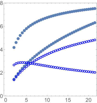
Figure 7: The regulated integrals $I_{1}$ (42) (lower curves at right ) and $I2$ (43) (upper curves) versus the momentum transfer $Q^{2}\,\,({\rm GeV}^{2})$. The closed points are for the flat distribution (p=0), the open points are for the asymptotic distribution (p=1). The values of the gluon mass and quark transverse energy used are $m_{\rm gluon}^{2}=1\,{\rm GeV}^{2},E_{\perp}^{2}=0.3\,{\rm GeV}^{2}$.

III.3 Scalar pion form factor from one-gluon exchange

The hard scalar (Higgs) block follows from the same diagrams (III.1) with the substitutions

$$(\epsilon(q)\cdot\gamma)\rightarrow 1,\,\,\,e_{q}\rightarrow\lambda_{q}$$

with the Yukawa couplings instead of the electric charges. To understand the nature of the scalar form factor in perturbation theory, and for simplicity, let us set the tensor DA $\varphi^{T}(x)=0$. With the same regulation procedure as used in the previous subsection, the result for the form factor is

$$S_{a}^{\pi}(Q^{2})\rightarrow -(\lambda_{u}+\lambda_{d})\bigg{[}\bigg{(}\frac{\pi C_{F}\alpha_{s}f_{\pi}^{2}\chi_{\pi}}{N_{c}Q^{2}}\bigg{)}\,\int_{0}^{1}dx_{1}dx_{2}\,\varphi_{\pi}(x_{1})\varphi_{\pi}^{P}(x_{2})$$ (44)

$$\times\bigg{(}\frac{1}{\overline{x}_{1}\overline{x}_{2}+m_{gluon}^{2}/Q^{2}}\bigg{)}\bigg{(}1+{1\over\overline{x}_{1}+E_{\perp}^{2}/Q^{2}}+\frac{1}{\overline{x}_{2}+E_{\perp}^{2}/Q^{2}}\bigg{)}\bigg{]}$$

Note that this term appears from the product of two different chiral components of the density matrix. It must be so because, unlike the interaction with the photon, the scalar vertex flips chirality, and therefore needs to be complemented by $another$ chirality flip.

Another contribution to the scalar form factor stems from the mass term in the quark propagators (III.1), $\sim M_{Q}/Q^{2}$, which we usually neglect. Since it also flips chirality, it generates a subleading contribution (as we assume $M_{Q}\ll\chi_{\pi}$)

$$S_{a}^{\pi}\rightarrow-(\lambda_{u}+\lambda_{d}) \bigg{[}\bigg{(}\frac{\pi C_{F}\alpha_{s}f_{\pi}^{2}M}{N_{c}Q^{2}}\bigg{)}\,\int_{0}^{1}dx_{1}dx_{2}\,\bigg{(}\varphi_{\pi}(x_{1})\varphi_{\pi}(x_{2})-{4\chi_{\pi}^{2}\over Q^{2}}\varphi_{\pi}^{P}(x_{1})\varphi_{\pi}^{P}(x_{2})\bigg{)}$$ (45)

$$\times\bigg{(}\frac{1}{\overline{x}_{1}\overline{x}_{2}+m_{gluon}^{2}/Q^{2}}\bigg{)}\bigg{(}{1\over\overline{x}_{1}+E_{\perp}^{2}/Q^{2}}+\frac{1}{\overline{x}_{2}+E_{\perp}^{2}/Q^{2}}\bigg{)}\bigg{]}$$

which we have not included in the results quoted above.

III.4 Gravitaton and dilaton pion form factors from one-gluon exchange

QCD is characterized by the symmetric energy momentum tensor

$$T^{\mu\nu}= \frac{2}{\sqrt{-g}}\frac{\delta S_{QCD}}{\delta{g_{\mu\nu}}}=F^{a\mu\lambda}F^{a\nu}_{\lambda}+\frac{1}{4}g^{\mu\nu}F^{2}+\frac{1}{2}\overline{\psi}\gamma^{[\mu}i\overleftrightarrow{D}^{\nu]_{+}}\psi$$ (46)

with the symmetric and long derivative $\overleftrightarrow{D}=\overrightarrow{D}-\overleftarrow{D}$, and $[]_{+}$ denotes symmetrization. It is conserved $\partial_{\mu}T^{\mu\nu}=0$, with a non-vanishing trace

$$T^{\mu}_{\mu}=\frac{\beta(g)}{2g}F_{\mu\nu}^{a}F^{a\mu\nu}+m\overline{\psi}\psi$$ (47)

due to the conformal anomaly, with the one-loop beta function $\beta(g)=-(11N_{c}/3-2N_{f}/3)g^{3}/16\pi^{2}$.

The form factor of the energy-momentum tensor in a pion (or any pseudoscalar) state is contrained by Lorentz symmetry, parity and energy-momentum conservation. Under these strictures it takes the general form

$$\left<p_{2}\left|T^{\mu\nu}\right|p_{1}\right>=\frac{1}{2}(g^{\mu\nu}q^{2}-{q^{\mu}q^{\nu}})\Theta_{1}(q^{2})+\frac{1}{2}{p^{\mu}p^{\nu}}\Theta_{2}(q^{2})$$ (48)

with $q^{\mu}=p^{\mu}_{2}-p_{1}^{\mu}$ and $p^{\mu}=p_{1}^{\mu}+p_{2}^{\mu}$. The two form factors correspond to the spin representations $1\otimes 1=0\oplus 1\oplus 2$ with $1$ excluded by parity. They reflect on the tensor exchange or graviton ($2$), and the scalar exchange or dilaton (0). The graviton form factor is described by $\Theta_{2}$, and the dilaton form factor is described by the trace

$$\left<p_{2}\left|T^{\mu}_{\mu}\right|p_{1}\right>=\frac{3}{2}q^{2}\Theta_{1}(q^{2})+\frac{1}{2}(4m_{\pi}^{2}-q^{2})\Theta_{2}(q^{2})$$ (49)

The normalization $\Theta_{2}(0)=1$ is fixed by recalling that $H=\int dx\,T^{00}$ is the Hamiltonian, with $\left<p_{1}\left|H\right|p_{1}\right>=p_{1}^{0}[2p_{1}^{0}(2\pi)\delta_{p}(0)]$. At low energy, the Goldstone nature of the pion allows to organize (46) in a momentum expansion

$$\left<p_{2}\left|T^{\mu\nu}\right|p_{1}\right>=p_{2}^{\mu}p_{1}^{\nu}+p_{2}^{\nu}p_{1}^{\mu}+\frac{1}{2}g^{\mu\nu}q^{2}+{\cal O}(p^{4})$$ (50)

which shows that the two invariant form factors normalize to 1, $\Theta_{1}(0)=\Theta_{2}(0)=1$. Note that in two-dimensions, there is only one invariant form factor for the dilaton, and an exact non-perturbative result can be derived in the context of the large $N_{c}$ limit Ji:2020bby.

In general, the invariant form factors $\Theta_{1,2}$ are fixed by the energy density $T^{00}$ and the trace identity (49)

$$-\frac{Q^{2}}{2}\Theta_{1}(Q^{2})+2\bigg{(}m_{\pi}^{2}+\frac{Q^{2}}{4}\bigg{)}\Theta_{2}(Q^{2}) =\left<p_{2}|T^{00}(0)|p_{1}\right>$$

$$-\frac{3Q^{2}}{2}\Theta_{1}(Q^{2})+2\bigg{(}m_{\pi}^{2}+\frac{Q^{2}}{4}\bigg{)}\Theta_{2}(Q^{2}) =\left<p_{2}|T^{\mu}_{\mu}(0)|p_{1}\right>$$ (51)

in the Breit frame with $q^{\mu}=(0,Q)$ and $p^{\mu}_{1,2}=(E_{p},\mp Q/2)$. More specifically, we have

$$\Theta_{1}(q^{2}) =\frac{1}{q^{2}}\left<p_{2}\left|\big{(}T^{\mu}_{\mu}(0)-T^{00}(0)\big{)}\right|p_{1}\right>\equiv\frac{1}{q^{2}}\big{(}T_{\mu\mu}^{\pi}(q^{2})-T_{00}^{\pi}(q^{2})\big{)}$$

$$\Theta_{2}(q^{2}) =\frac{1}{q^{2}-4m^{2}_{\pi}}\left<p_{2}\left|\big{(}T^{\mu}_{\mu}(0)-3T^{00}(0)\big{)}\right|p_{1}\right>\equiv\frac{1}{q^{2}-4m_{\pi}^{2}}\big{(}T_{\mu\mu}^{\pi}(q^{2})-3T_{00}^{\pi}(q^{2})\big{)}$$ (52)

with $q^{2}=-Q^{2}$. We identify the strength of the graviton coupling as $-3T^{00}+T^{\mu}_{\mu}$ from (III.4), and the strength of the dilaton coupling as $T^{\mu}_{\mu}$ from (49).

The hard graviton and dilaton blocks follow from the same diagrams (III.1) using the elementary quark vertices in (46)

$$\left<f(k_{1}+q)\left|\frac{1}{2}\overline{\psi}\gamma^{[\mu}i\overleftrightarrow{\partial}^{\nu]_{+}}\psi(0)\right|f(k_{1})\right> =\frac{1}{2}\gamma^{[\mu}(2k_{1}+q)^{\nu]_{+}}$$

$$\left<f(k_{2})\left|\frac{1}{2}\overline{\psi}\gamma^{[\mu}i\overleftrightarrow{\partial}^{\nu]_{+}}\psi(0)\right|f(k_{2}-q)\right> =\frac{1}{2}\gamma^{[\mu}(2k_{2}-q)^{\nu]_{+}}$$ (53)

for $f=u,d$. The $00$-coupling corresponds to the vertex $\gamma^{0}(2k_{1,2}\pm q)^{0}$, and the $\mu\mu$-coupling corresponds to the vertex $(2\not{k}_{1,2}\pm\not{q})$. With this in mind, the corresponding perturbative contributions to the pion after regularization are listed in (II.5). The non-perturbative contributions in the context of semi-classics will follow.

III.5 The form factor of the transversely polarized
rho meson from one-gluon exchange

The perturbative and unregulated contribution to the vector form factor for the rho meson with transverse polarization, can be obtained through similar contractions. For instance, if we set in this case the axial DA amplitude $\varphi_{\rho}^{A}=0$, then a typical perurbative contribution to the rho vector form factor follows from the vector insertion

$$V_{a}^{\rho}(Q^{2})\rightarrow -\frac{e_{u}C_{F}}{N_{c}}\int_{0}^{1}\,dx_{1}\,dx_{2}\,\bigg{(}\frac{-1}{-\bar{x}_{1}\bar{x}_{2}Q^{2}}\bigg{)}$$ (54)

$$\times{\rm Tr}\bigg{[}\epsilon_{T}(q)\cdot\gamma\,\bigg{(}\frac{{\not{p}}^{\prime}-\overline{x}_{1}\not{p}}{-\bar{x}_{1}Q^{2}}\bigg{)}\,g_{s}\gamma^{\alpha}\,\gamma^{0}\bigg{(}-\frac{i}{4}\not{\epsilon}^{\prime}_{T}({f_{\rho}}m_{\rho}\,\varphi_{\rho}(x_{1})+{f^{T}_{\rho}}\not{p}^{\prime}\,\varphi^{T}_{\rho}(x_{1}))\bigg{)}^{\dagger}\gamma^{0}$$

$$\qquad\times g_{s}\gamma_{\alpha}\bigg{(}-\frac{i}{4}\not{\epsilon}_{T}({f_{\rho}}m_{\rho}\,\varphi_{\rho}(x_{2})+{f^{T}_{\rho}}\not{p}\,\varphi^{T}_{\rho}(x_{2}))\bigg{)}\bigg{]}$$

Since $\gamma^{\alpha}\not{\epsilon}^{\prime}_{T}\not{p}^{\prime}\gamma_{\alpha}=4\epsilon_{T\mu}^{\prime}p^{\prime\mu}=0$, the tensor contribution $\not{\epsilon}_{T}\not{p}$ drops out in the spin trace. The final result with all insertions combined is subleading in $m_{\rho}^{2}/Q^{2}$

$$V_{a}^{\rho}(Q^{2})\rightarrow -\epsilon_{\mu}(q)(p^{\mu}+p^{\prime\mu})\,(e_{u}+e_{\overline{d}})\,\epsilon^{\prime*}_{T}\cdot\epsilon_{T}\,\bigg{[}\bigg{(}\frac{2\pi C_{F}\alpha_{s}f_{\rho}^{2}m_{\rho}^{2}}{N_{c}Q^{4}}\bigg{)}$$ (55)

$$\times\int_{0}^{1}dx_{1}dx_{2}\,\varphi_{\rho}(x_{1})\varphi_{\rho}(x_{2})\bigg{(}\frac{1}{\overline{x}_{1}\overline{x}_{2}}\bigg{(}\frac{1}{2}\bigg{(}\frac{1}{\overline{x}_{1}}+\frac{1}{\overline{x}_{2}}\bigg{)}-1\bigg{)}\bigg{]}$$

Similar arguments applied to the scalar form factor of the transversely polarized vector meson yield the unregulated result

$$S_{a}^{\rho}(Q^{2})\rightarrow (\lambda_{u}+\lambda_{\overline{d}})\,M_{Q}\,\epsilon^{\prime*}_{T}\cdot\epsilon_{T}\bigg{[}\bigg{(}\frac{\pi C_{F}\alpha_{s}}{N_{c}}\,\frac{m_{\rho}f_{\rho}f^{T}_{\rho}}{M_{Q}Q^{2}}\bigg{)}$$ (56)

$$\times\int dx_{1}dx_{2}\,\frac{1}{\overline{x}_{1}\overline{x}_{2}}\bigg{(}\frac{1}{\overline{x}_{2}}\varphi_{\rho}(x_{1})\varphi^{T}_{\rho}(x_{2})+\frac{1}{\overline{x}_{1}}\varphi_{\rho}(x_{2})\varphi^{T}_{\rho}(x_{1})\bigg{)}\bigg{]}$$

The full perturbative results including the axial DA $\varphi_{\rho}^{A}$ are quoted in the results section above.

III.6 Including other NJL-type local 4-fermion operators?

In the spirit of the effective scattering theory for quarks, one may think of introducing $all$ local operators of the type

$${\cal O}_{\Gamma}\equiv(\bar{q}\Gamma q)(\bar{q}\Gamma q)$$

where the matrices $\Gamma$ include all possible Dirac, color and flavor structures. Naively, including any of them is rather straightforward. The obvious practical problem is due to the fact that total basis of all operators is way too large for meaningful applications. One needs an organizational principle for the selection of only relevant ones, to be kept in the hard block.

From short distances, one-gluon exchange corresponds to the product of two color currents, with $\Gamma=\gamma_{\mu}\tau^{a}/2$. Colorless exchanges start from two gluons, or perhaps scalar and tensor glueballs (in the discussion section we will explain why the latter seems to be especially important, based on high energy scattering phenomenology). If so, $\Gamma=1$ or the stress tensor $\Gamma_{T}=i\partial_{\mu}\gamma_{\nu}$.

From large distance perspective, one may think about mesonic exchanges, as is done for nuclear forces. If this is the case, colorless scalar, pseudoscalar and vector $\Gamma$ should be used, with or without flavor matrices. Still, the basis is too large for this approach to be practical.

Instantons generate a very specific effective quark-quark interactions. The most prominent is the one discovered by ’t Hooft ’t Hooft (1976). It provides a unique nontrivial selection of matrices, and so, in this work, we have focused on this particular choice. The organizational principle is the use of semi-classics in the hard block supplemented by a perturbative correction (one-loop).

III.7 Born-style estimates of the instanton effects

This section is devoted to estimate of the diagram (b) of Fig. 1. Note that the point in which the hard photon (scalar) is absorbed is separated, by a quark propagator, from the location of the quark-antiquark scattering. (On general grounds, one may question why such a separation is always possible, and in fact we will not assume it in the next section.)

In this warm-up section, we include the instanton field in the “naive Born-like approximation”, just by substituting the gluon propagator by the (Fourier transform) of the instanton field. The reader must be warned that such approach is a “naive estimate” of the effect, similar in spirit to our treatment of the NJL vertex above. However, we note that the instanton field is nonperturbative, $gA_{\mu}\sim O(1)$ in the weak coupling $g\ll 1$ regime. Therefore, a consistent treatment should include the instanton field in the full quark propagator to all orders, with all zero and nonzero modes, through the instanton, a task relegated to later sections below.

Before we start, let us mention the issue of gauge selection. Historically, the instantons were discovered in the so called “regular” gauge, in which the topological singularity is at infinity. In contrast, the so called ”singular” gauge put it at the origin. The difference between them became apparent in any discussion of multi-instanton configurations (and ensembles): only the singular ones can be used, since there is only one infinity for all of them. This is important for our estimate, since the point-like gauge singularity will show up in the Fourier transform.

With this in mind, the instanton field has the form

$$(A_{\mu}(x))^{i}_{j}(x)=-\frac{i}{2g}U^{i}_{\alpha}(\sigma_{\mu}\overline{x}-x\overline{\sigma}_{\mu})^{\alpha}_{\beta}U^{\dagger\beta}_{j}\frac{\rho^{2}}{x^{2}(x^{2}+\rho^{2})}$$

$$(A_{\mu}(x))^{i}_{j}(x)=+\frac{i}{2g}U^{i}_{\alpha}(\sigma_{\mu}\overline{x}-x\overline{\sigma}_{\mu})^{\alpha}_{\beta}U^{\dagger\beta}_{j}\frac{\rho^{2}}{(-x^{2}+i0)(-x^{2}+i0+\rho^{2})}$$ (57)

in Euclidean and Minkowski space respectively. In Euclidean space, the Fourier transform of the instanton is

$$A_{\mu}^{a}(k)=\frac{(2\pi\rho)^{2}}{2g}{\rm Tr}(T^{a}U(\sigma_{\mu}\overline{k}-k\overline{\sigma}_{\mu})U^{\dagger})\frac{\mathbb{G}(\rho\sqrt{q^{2}})}{k^{2}}=\frac{i(2\pi\rho)^{2}}{g}{D^{ab}(U)\overline{\eta}^{b}_{\mu\nu}k^{\nu}}\frac{\mathbb{G}(\rho\sqrt{q^{2}})}{k^{2}}$$

with the field form factor

$$\mathbb{G}(\rho\sqrt{k^{2}})=\bigg{(}\frac{4}{k^{2}\rho^{2}}-2K_{2}(\rho\sqrt{k^{2}})\bigg{)}$$ (59)

which is normalized to 1, $\mathbb{G}(0)=1$. (No minus sign under the root because here we use Euclidean notations.) The D-function is $D^{ab}(U)={\rm Tr}(T^{a}U\tau^{b}U^{\dagger})$ with the normalization ${\rm Tr}(T^{a}T^{b})=\delta^{ab}/2$. In particular, the analytical continuation of (III.7) to Minkowski space with amputation gives

$$\lim_{k^{2}\rightarrow 0}(-k^{2})\,\epsilon^{\mu}(k)A_{\mu}^{a}(k)= -\frac{2\pi^{2}\rho^{2}}{g}{\rm Tr}\bigg{(}T^{a}\,U(\epsilon(k)\overline{k}-k\overline{\epsilon}(k))U^{\dagger}\bigg{)}\,\mathbb{G}(0)$$

$$\rightarrow -i\frac{(2\pi\rho)^{2}}{g}\,{D^{ab}(U)\overline{\eta}^{b}_{\mu\nu}\epsilon^{\mu}(k)k^{\nu}}$$ (60)

Note that the 2-point gluon correlator in both spaces read

$$A_{\mu}^{a}(k)A_{\nu}^{b}(-k)=\frac{(2\pi\rho)^{4}}{g^{2}}D^{ac}(U)D^{bd}(U)\frac{\overline{\eta}^{c}_{\mu\alpha}\overline{\eta}^{d}_{\nu\beta}k^{\alpha}k^{\beta}}{k^{4}}\,\mathbb{G}^{2}(\rho\sqrt{k^{2}})$$ (61)

The non-perturbative contribution to the mesonic form factor in the Born approximation illustrated in Fig. 1b, can be evaluated using the single instanton contribution in (61). This contribution corresponds to the instanton (anti-instanton) effect on a pair of non-zero quark modes. For light quarks, it is subleading in diluteness with the contribution shown in Fig. 1c which involves non-zero mode contributions. For heavy quarks it is the sole and dominant non-perturbative contribution.

The non-perturbative gluon propagator (61) when averaged over an instanton plus anti-instanton contribution gives

$$\Delta_{\mu\nu}^{ab}(k)= \bigg{<}A_{\mu}^{a}(k)A_{\nu}^{b}(-k)\bigg{>}_{I+\overline{I}}$$

$$= \frac{n}{2}\frac{(2\pi\rho)^{4}}{g_{s}^{2}}\bigg{<}D^{ac}(U)D^{bd}(U)\bigg{>}_{U}\,\bigg{(}\overline{\eta}^{c}_{\mu\alpha}\overline{\eta}^{d}_{\nu\beta}+{\eta}^{c}_{\mu\alpha}{\eta}^{d}_{\nu\beta}\bigg{)}\frac{k^{\alpha}k^{\beta}}{k^{4}}\,\mathbb{G}^{2}(\rho\sqrt{k^{2}})$$

$$\rightarrow -\delta^{ab}\,\frac{n(2\pi\rho)^{4}}{g_{s}^{2}}\frac{g_{\mu\nu}k^{2}-k_{\mu}k_{\nu}}{k^{4}}\,\mathbb{G}^{2}(\rho\sqrt{-k^{2}})\equiv\delta^{ab}\Delta_{\mu\nu}(k)$$ (62)

with the last relation following in Minkowski space. The contribution of Fig. 1b follows that in Fig. 1a in the form (III.1) with the substitution of (III.7) for the gluon propagator, namely

$$\frac{-g_{\mu\nu}}{({k}_{1}-{k}_{2})}\rightarrow\Delta_{\mu\nu}({k}_{1}-{k}_{2})\qquad\frac{-g_{\mu\nu}}{(\underline{k}_{1}-\underline{k}_{2})}\rightarrow\Delta_{\mu\nu}(\underline{k}_{1}-\underline{k}_{2})$$ (63)

IV Instanton-induced effects

IV.1 From non-zero-mode propagators to hard block operators

As we already discussed, the instanton field is nonperturbative, or strong $A_{\mu}\sim 1/g$. Therefore even if the coupling $g$ is small, it cancels out. The propagation in such field cannot be calculated in powers of $g$. Instead, one should use the fully dressed (re-summed) propagators. With this in mind, the next step is the identification of the hard block, via the “amputation” of the free propagators also known as Lehmann-Symanzik-Zimmermann (LSZ) reduction. We start explaining how this procedure works in the coordinate representation, starting from the simpler case of spinless (scalar) quarks, as discussed in Shuryak and Velkovsky (1994).

The propagator for a massless scalar particle in an instanton field has the form Brown et al. (1978)

$$\Delta(x,y)=\Delta_{0}(x-y)\bigg{(}1+\rho^{2}\frac{[Ux\bar{y}U^{\dagger}]}{x^{2}y^{2}}\bigg{)}\frac{1}{(\Pi(x)\Pi(y))^{\frac{1}{2}}}$$ (64)

with $\Delta_{0}(x)=1/(2\pi x)^{2}$ the free scalar propagator, and $\Pi(x)=1+\rho^{2}/x^{2}$, and $x,\bar{y}$ are convoluted with (Euclidean 4d) sigma matrices (B). To see how the LSZ reduction operates on (64), we consider the limit $x,y\gg\rho$, which is dominated by the asymptotic of $1/\sqrt{\Pi(x)}\approx(1-\rho^{2}/2x^{2}+...)$. For a single quark line, the color averaging in (64) yields

$$\left<[Ux\bar{y}U^{\dagger}]\right>_{U}=\frac{x\cdot y}{N_{c}}$$ (65)

Inserting (65) and keeping only the asymptotic contributions, give

$$\Delta(x-y)\approx\Delta_{0}(x-y)\bigg{[}1-\frac{\rho^{2}}{2x^{2}y^{2}}\bigg{(}(x-y)^{2}+2x\cdot y\bigg{(}1-\frac{1}{N_{c}}\bigg{)}\bigg{)}\bigg{]}$$ (66)

one finds that the term of order $\rho^{2}$ in the numerator becomes exactly the combination $(x-y)^{2}$ in the denominator, so that it is canceled out. Subtracting the free propagator, one observes that the $O(\rho^{2})$ lowest-order instanton contribution is proportional to $1/x^{2}y^{2}=(4\pi^{2})^{2}D_{0}(x)D_{0}(y)$, just the product of Green function describing free propagation to and from the instanton. So, in this case the LSZ procedure is just an “amputation” of these free propagators.

This result can be generalized to an “amputated line operator”, in the momentum representation with arbitrary in- and out-momenta

$${\cal T}(k,k^{\prime})=\int d^{4}xd^{y}e^{ikx-ik^{\prime}y}\big{(}\partial_{x}^{2}\Delta(x,y)\partial_{y}^{2}\big{)}$$ (67)

where the second derivatives over $x$ and $y$ stand for the “amputation” of the trivial large distance part of the Green function. Out of those one can construct n-body scattering amplitudes by taking their powers, averaging over the positions of the instanton center $z_{\mu}$ and tracing over the color indices

$${\cal A}(k_{i},k^{\prime}_{i})={\rm Tr}\bigg{[}\prod_{i=1}^{n}{\cal T}(k_{i},k^{\prime}_{i})\bigg{]}$$ (68)

The simplest of them, n=1, leads to the forward scattering amplitude on the instanton

$$T(k,k)=\frac{4\pi^{2}\rho^{2}}{N_{c}}$$ (69)

used by one of us long ago, in Shuryak (1982b). This result explains the instanton suppression term at finite temperatures previously calculated in Pisarski and Yaffe (1980), and allowed its generalization to the case of finite temperature and density. The n=2 case corresponds to two-by-two scattering, n=3 to three-by-three scattering, and so on. Averaging over the instanton position leads to momentum conservation $\sum_{i}k_{i}=\sum k^{\prime}_{i}$. The former case is important for meson form factors, the latter for baryon ones.

The remaining important detail is that in Euclidean calculations $k=\sqrt{k_{\mu}^{2}}$ where all coordinates appear with plus sign. Going to Minkowski kinematics with “on-shell” $k\rightarrow 0$, partons can only mean here all components going to zero, or $x,y$ go to large distances . The scattering amplitude one gets from this procedure is just a constant, corresponding to low energy local interaction. There is no correlation between $k,k^{\prime}$ momenta, or any angular distribution. There is no nonlocality or explicit form factors in this procedure, and thus no dependence on the momentum transfer $k-k^{\prime}$ in quark-antiquark scattering.

The extension of the (massless) scalar case to the (massless) spinor case is done by using the full quark non-zero mode propagator in the chiral-split form Brown et al. (1978)

$$S_{NZ}(x,y)= \overrightarrow{D/\hskip 2.58334pt_{x}}\Delta(x,y){1+\gamma_{5}\over 2}+\Delta(x,y)\overleftarrow{D/\hskip 2.58334pt}_{y}{1-\gamma_{5}\over 2}$$

$$= \overline{S}(x,y)\frac{1+\gamma_{5}}{2}+{S}(x,y)\frac{1-\gamma^{5}}{2}$$ (70)

with the free Weyl propagators $S_{0}=1/\overline{\partial}$ and $\overline{S}_{0}=1/{\partial}$, in the notations detailed in Appendix B. The long derivative $\not{D}=\not{\partial}-i\not{A}$ acts on the left and right respectively of the (massless) scalar propagator, with each explicit contribution

$$\overline{S}(x,y)=\bigg{(}\overline{S}_{0}(x-y)\bigg{(}1+\rho^{2}\frac{[Ux\bar{y}U^{\dagger}]}{x^{2}y^{2}}\bigg{)}+\frac{\rho^{2}\overline{\sigma}_{\mu}}{4\pi^{2}}\frac{[Ux\overline{\sigma}_{\mu}(x-y)\bar{y}U^{\dagger}]}{\Pi_{x}x^{4}(x-y)^{2}y^{2}}\bigg{)}\,\frac{1}{(\Pi_{x}\Pi_{y})^{\frac{1}{2}}}$$

$$S(x,y)=\bigg{(}S_{0}(x-y)\bigg{(}1+\rho^{2}\frac{[Ux\bar{y}U^{\dagger}]}{x^{2}y^{2}}\bigg{)}+\frac{\rho^{2}\sigma_{\mu}}{4\pi^{2}}\frac{[Ux(\bar{x}-\bar{y})\sigma_{\mu}\bar{y}U^{\dagger}]}{x^{2}(x-y)^{2}y^{4}\Pi_{y}}\bigg{)}\,\frac{1}{(\Pi_{x}\Pi_{y})^{\frac{1}{2}}}$$ (71)

and with $U$ valued in $SU(N_{c})$. When a mixture of color and spinor indices occurs, the spinor matrices act on the upper left corner of the $N_{c}\times N_{c}$ color matrices. Recall that the terms without and with the bar here correspond to Weyl notations with two-by-two matrices. They do not correspond to quarks and antiquarks – the diagonal of $\gamma_{0}$ – but to the left and right quark polarizations, diagonal of $\gamma_{5}$. These notations are compatible with other Weyl-style notations used.

In the case of a scalar (Higgs) probe on a $q\bar{q}$ meson pair, the chirality of the quark is flipped, and therefore one part of the diagram contributes

$$\bar{S}(x,z)S(z,y)+S(x,z)\bar{S}(z,y)\,,$$

in which case the endpoints $x,y$ should be taken to large distances while the intermediate point $z$ is still residing inside the instanton field. In the former term the covarient derivatives, acting from both sides, create free fermionic propagators, which can be readily amputated. What is left, depending on the point $z$ is just the factor $1/\Pi_{z}$. Its Fourier transform with momentum transfer $q_{\mu}$ is

$$\int{d^{4}z}\,{e^{iq\cdot z}\over\Pi_{z}}$$ (72)

Unfortunately, this is not so simple in the second part of the diagram. The second term of $S(x,z)$ at large $x$ is of order $1/x^{2}$, with a power not matching the free fermion propagator $S_{0}\sim x/x^{4}$. It means that the LSZ reduction in coordinate representation is not local. Let us use the following trick: multiply and divide by $D/\hskip 2.58334pt$. The $D/\hskip 2.58334pt$ in the numerator now reproduces the free propagator, which we can amputate. The $D/\hskip 2.58334pt$ in the denominator will become the negative power of momentum in the amplitude when taken to the momentum representation, generating a $negative$ moment of the wave function by convolution to the wavefunction.

Now let us focus on the line in which there is no external probe. There is a single $S(x,y)$ in which $both$ coordinates are taken to infinity. Again, in each term one dependence leads to a straightforward LSZ procedure, and the other lacks one power of the distance. We use the same trick and represent it as $D/\hskip 2.58334pt_{x}\Delta D/\hskip 2.58334pt_{y}(1/D/\hskip 2.58334pt_{y})$. The effective amplitude takes the form ${\cal A}\sim\rho^{2}({1\over x}+{1\over x^{\prime}})$. We now proceed to give a more quantitative derivation of these results.

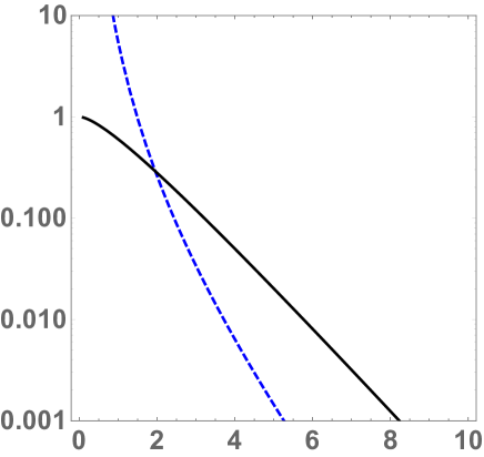
Figure 8: The blue dashed and the solid black lines correspond to the functions $F_{1}(Q\rho)$ and $F_{2}(Q\rho)$ versus $Q$ as given in (LABEL:eqn_F2), respectively.

The LSZ reduced non-zero mode contributions to the $q\overline{q}$ vector vertex with polarization $\epsilon_{\mu}(q)$, can be formally written in the chiral split form as

$$\left<\left<k_{2}\left|{\partial}\,\overline{S}\,\overline{\epsilon}(q)\,\overline{S}\,{\partial}\,\frac{1+\gamma_{5}}{2}+\overline{\partial}\,{S}\,{\epsilon}(q)\,{S}\,\overline{\partial}\,\frac{1-\gamma_{5}}{2}\right|k_{1}\right>\otimes\left<\underline{k}_{1}\left|{\partial}\,\overline{S}\,{\partial}\,\frac{1+\gamma_{5}}{2}+\overline{\partial}\,{S}\,\overline{\partial}\,\frac{1-\gamma_{5}}{2}\right|\underline{k}_{2}\right>\right>_{U}$$

where the overall averaging over color is indicated by the subscript $U$, and the mass shell conditions $k_{1,2}^{2}\rightarrow 0$ and $\underline{k}_{1,2}^{2}\rightarrow 0$ are subsumed. Using the results in Appendix D, the final vector vertex follows by adding (D) to the color averaged (164) and combining the result with (169) to finally obtain

$$\bigg{[}2\kappa\mathbb{G}_{V}(q\rho)\overline{u}(k_{2})\not{\epsilon}(q)u(k_{1})\bigg{]}\times\bigg{[}\bigg{(}{{2\pi^{2}\rho^{2}}}\bigg{)}\overline{d}(\underline{k}_{1})\bigg{(}\frac{1}{\not{\underline{k}}_{1}}+\frac{1}{\not{\underline{k}}_{2}}\bigg{)}d(\underline{k}_{2})\bigg{]}$$

The induced vector form factor ${\mathbb{G}}_{V}$ consists of two parts

$${\mathbb{G}}_{V}(\xi)=F_{1}(Q\rho)+{1\over N_{c}M^{2}\rho^{2}}F_{2}(Q\rho)$$ (75)

with specifically

$$F_{1}(x)\equiv\bigg{(}\frac{K_{1}(x)}{x}\bigg{)}^{\prime\prime}= {1\over 4x^{3}}(4xK_{0}(x)+(8+3x^{2})K_{1}(x)+x(4K_{2}(x)+xK_{3}(x)))$$

$$F_{2}(x)\equiv x\bigg{(}\frac{(xK_{1})^{\prime}}{x}\bigg{)}^{\prime}= {1\over 4x}(-2xK_{0}(x)+(-4+3x^{2})K_{1}(x)+x(-2K_{2}(x)+xK_{3}(x)))\equiv xK_{1}(x)$$

We have summed over $n/2$ instantons plus $n/2$ anti-instantons, analytically continued to Minkowski signature, and dropped the extra factor of $i$ since (IV.1) follows from $S=1+iT$ with $T$ identified with the vector vertex. Overall momentum conservation follows from the Z-integration over the instanton and anti-instanton positions leading to $q+k_{1}+\underline{k}_{1}=k_{2}+\underline{k}_{2}$ for the 2-body vertex (IV.1). In Fig. 8 the behavior of $F_{1,2}(Q\rho)$ in (LABEL:eqn_F2) is shown, with $F_{2}(Q\rho)$ dominant at large $Q$.

After the hard block is defined, one carries the trace with the pion (or rho) density matrices. The propagators remaining in the second bracket of (IV.1) are treated as follows

$${1\over\not{\underline{k}}_{1}}\rightarrow{\not{\underline{k}}_{1}\over M_{Q}^{2}}$$

with $M_{Q}$ being the constituent quark mass. The final expression is (16).

We have checked that similar arguments apply to the scalar form factor, which is seen to mix chirality through $S\overline{S}$ and $\overline{S}S$ contributions, but the result is found to be identical to (158) with the substitution $\not{\epsilon}(q)\rightarrow 1$ and no additional contribution. Hence, the same result holds for the scalar vertex with the substitution $\not{\epsilon}(q)\rightarrow 1$ in (IV.1) and the induced scalar form factor

$$\mathbb{G}_{V}(\xi)\rightarrow{\mathbb{G}}_{S}(\xi)=\bigg{(}\frac{K_{1}(\xi)}{\xi}\bigg{)}^{\prime\prime}$$ (77)

Note that the two terms in (75) have opposite signs. So their sum is sensitive to the averaging over the instanton size (see section IV.10). Fig.9 displays the contribution of each of them, as well as their sum. After convolution of the hard block with the pion density matrices we get the final result for $V_{c}^{\pi}$, as given in (16).

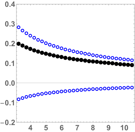
Figure 9: The nonzero mode contributions to the vector pion form factor times $Q^{2}\,({\rm GeV}^{2})$, versus $Q^{2}\,({\rm GeV}^{2})$. The blue circle above and below show the contributions of $\langle F_{1}\rangle_{\rho}$ and $\langle F_{2}\rangle_{\rho}$, respectively. The black closed circles are their sum.

IV.2 The non-zero mode contributions to the rho vector form factors

The general decomposition of the vector form factor of the rho meson compatible with parity, time-reversal symmetry and Lorentz symmetry is of the form

$$\left<\rho(p^{\prime},\epsilon^{\prime})\left|J_{\mu}(0)\right|\rho(p,\epsilon)\right> =F_{V}(q^{2})\,\epsilon^{\prime*}\cdot\epsilon\,(p_{\mu}+p_{\mu}^{\prime})$$ (78)

$$+\frac{G_{V}(q^{2})}{2m_{\rho}}\,\left(\epsilon^{*\prime}_{\mu}\epsilon\cdot q-\epsilon_{\mu}\epsilon^{*\prime}\cdot q\right)+\frac{H_{V}(q^{2})}{4m_{\rho}^{2}}\,\epsilon^{\prime*}\cdot q\epsilon\cdot q\,(p_{\mu}+p_{\mu}^{\prime})$$

with $F_{V},H_{V}$ contributing to the electric form factor and $G_{V}$ to the magnetic form factor of the rho.

The contribution to the vector form factor of the transverse rho meson in the large momentum limit, involves all three form factors in (78) in general. For simplicity, we focus on the contribution to the electric part $F_{V}$ by choosing the transverse polarization $\epsilon_{T}(p,p^{\prime})$ of the $\rho_{\perp}$ with momentum $p,p^{\prime}$ to be also transverse to $q$, or $\epsilon_{T}(p,p^{\prime})\cdot q=0$. In the large momentum limit and for the axial DA $\varphi^{A}(x)=0$ for simplicity, the unregulated contribution to $F_{V}$ is

$$V_{c}^{\rho}(Q^{2})\rightarrow -\epsilon_{\mu}(q)(p^{\mu}+p^{\prime\mu})\,\epsilon^{\prime*}_{T}\cdot\epsilon_{T}\,(e_{u}+e_{\overline{d}})\,\bigg{[}\frac{\kappa\pi^{2}{f}^{T2}_{\rho}}{N_{c}}\,\left<\rho^{2}\mathbb{G}_{V}(Q\rho)\right>\int_{0}^{1}dx_{1}dx_{2}\,$$

$$\times\bigg{(}\bigg{(}\frac{1}{\overline{x}_{1}}+\frac{1}{\overline{x}_{2}}\bigg{)}\varphi^{T}_{\rho}(x_{1})\varphi^{T}_{\rho}(x_{2})+\frac{1}{2}\frac{f_{\rho}^{2}m_{\rho}^{2}}{{f}_{\rho}^{T2}M_{Q}^{2}}\varphi_{\rho}(x_{1})\varphi_{\rho}(x_{2})\,(\overline{x}_{1}+\overline{x}_{2})\bigg{)}\bigg{]}$$

IV.3 The non-zero mode contribution to the rho scalar form factors

The general decomposition of the scalar form factor of the rho meson compatible with parity, time-reversal symmetry and Lorentz symmetry is of the form

$$\left<\rho(p^{\prime},\epsilon^{\prime})\left|S(0)\right|\rho(p,\epsilon)\right>=F_{S}(q^{2})\,\epsilon^{\prime*}\cdot\epsilon+\frac{H_{S}(q^{2})}{4m_{\rho}^{2}}\,\epsilon^{\prime*}\cdot q\epsilon\cdot q$$ (80)

Similarly to the pion scalar form factor, the contribution to the scalar form factor of the longitudinal rho meson vanishes because of a poor spin trace. As a result, the invariant scalar form factors in (80) satisfy

$$F_{S}(q^{2})-\frac{q^{4}}{16m_{\rho}^{4}}H_{S}(q^{2})\approx 0$$ (81)

in the large momentum limit. We can extract $F_{S}(q^{2})$ from the transversely polarized $\rho$ by choosing $\epsilon_{T}(p,p^{\prime})\cdot q=0$. For simplicity, if we set the axial DA amplitude $\varphi^{A}(x)=0$, the unregulated result is

$$S_{c}^{\rho}(Q^{2})\rightarrow (\lambda_{u}+\lambda_{\overline{d}})\,\epsilon_{T}^{\prime*}\cdot\epsilon_{T}\,M_{Q}\,\bigg{[}\frac{\kappa\pi^{2}f_{\rho}f^{T}_{\rho}}{2N_{c}}\frac{m_{\rho}}{M_{Q}}\,\left<\rho^{2}\mathbb{G}_{S}(Q\rho)\right>\int_{0}^{1}dx_{1}dx_{2}\,$$

$$\bigg{(}\varphi^{T}_{\rho}(x_{1})\varphi_{\rho}(x_{2})\bigg{(}\frac{1}{\overline{x}_{1}}+\frac{q^{2}}{M_{Q}^{2}}\overline{x}_{2}\bigg{)}+\varphi^{T}_{\rho}(x_{2})\varphi_{\rho}(x_{1})\bigg{(}\frac{1}{\overline{x}_{2}}+\frac{q^{2}}{M_{Q}^{2}}\overline{x}_{1}\bigg{)}\bigg{)}\bigg{]}$$

IV.4 The non-zero mode contribution to the graviton and dilaton
form factor of the pion

The instanton and anti-instanton contributions to the hard block with the energy-momentum tensor vertex, follows a similar reasoning as that for the vector insertion with the substitutions

$$\epsilon^{\mu}(q)\rightarrow(2k_{1,2}^{\mu}+q^{\mu}),\,\,\,e_{q}\rightarrow 1$$

and symmetrization. In particular, the non-zero mode contributions to the energy-momentum vertex follow from (IV.1) in the form

$$\bigg{[}2\kappa\mathbb{G}_{V}(Q\rho)\overline{u}(k_{2})(k_{1}+k_{2})^{[\mu}\gamma^{\nu]_{+}}u(k_{1})\bigg{]}\times\bigg{[}\bigg{(}{{2\pi^{2}\rho^{2}}}\bigg{)}\overline{d}(\underline{k}_{1})\bigg{(}\frac{1}{\not{\underline{k}}_{1}}+\frac{1}{\not{\underline{k}}_{2}}\bigg{)}d(\underline{k}_{2})\bigg{]}$$ (83)

with the induced vector form factor ${\mathbb{G}}_{V}$ given in (75-LABEL:eqn_F2). The non-zero mode vertex (83) when sandwiched betwen the pion DA yields (II.5).

IV.5 Quark zero modes and ’t Hooft effective Lagrangian

The quark propagator in the instanton background when expressed in the eigenmode basis, is a sum over all modes. In this section we focus on the specific term of this sum containing the zero modes. For a single instanton, this contribution takes the form

$$S_{Z}(x,y)={\psi_{0}(x)\psi^{*}_{0}(y)\over im_{q}}$$ (84)

with zero eigenvalue plus the quark mass in the denominator. This appears singular in the chiral limit $m_{q}\rightarrow 0$, but, as explained by ’t Hooft, since the amplitude for a single instanton is itself proportional to the product of masses of all light quark flavors, $\sim\prod_{q=u,d,s}m_{q}$, the Green functions and vertices with $N_{f}$ fermions are finite. This is how the famous ’t Hooft effective Lagrangian was derived.

In “empty” (perturbative) vacuum the mass here is that from QCD Lagrangian. However, when an instanton is not in the perturbative but rather in $physical$ QCD vacuum, the problem is more complex. A nonzero quark condensate makes the instanton amplitude nonzero even in the chiral limit. The current quark mass $m$ is supplemented by the so called “determinantal mass” $M^{*}$ Shifman et al. (1980)

$$M^{*}\equiv{2\pi^{2}\over 3}|\langle\bar{q}q\rangle|\rho^{2}\approx 200\,{\rm MeV}\bigg{(}{\rho\over\rho_{0}}\bigg{)}^{2}$$ (85)

(Note that this is $not$ the on-shell quark mass at zero momentum, which is about twice larger.) This mass was used in the first mean-field-style treatment of the instanton ensemble Shuryak (1982a), appending the quark masses both in the instanton determinant and in the denominator of the quark propagator.

After the formalism of the interacting instanton liquid model (IILM) was further developed, the so called “single instanton approximation” (SIA) for treating effects produced by a single member of the ensemble was further discussed in Ref.Faccioli and Shuryak (2001). It was pointed out there that the OPE expression from Shifman et al. (1980) was derived assuming factorization of the VEVs of 4-fermion operators in the QCD vacuum, which is also a version of the mean-field treatment. However, the instanton ensemble is highly correlated, and the expectation values of different multi-quark operators are highly inhomogeneous, and therefore the mean-field-style approximations are quite inaccurate. In particular, the operators of the type of ’t Hooft Lagrangian under consideration

$$\langle(\bar{u}u)(\bar{d}d)\rangle\gg\langle(\bar{u}u)\rangle\langle(\bar{d}d)\rangle$$

have strongly enhanced VEVs. The quark propagator in the QCD vacuum, is approximated by the form

$$S(x,y)=S_{Z}(x,y)+\sum_{I,J}\psi_{0I}^{*}(x)\bigg{(}{1\over T}\bigg{)}_{I,J}\psi_{0J}(y)$$ (86)

where $T_{IJ}$ denotes the so called “instanton hopping” matrix, constructed out of the Dirac zero modes overlaps between neighboring instantons $I,J$. Note that here enters the $inverse$ matrix, as propagators are inverse to Dirac operators. So, when one discusses a process in which both points $x,y$ are inside one instanton $I^{*}$, like when defining the hard block here, we can restrict the sum to only the term with the zero mode of this very instanton. This leads to the following redefinition of the “determinantal mass”

$${1\over M_{u}}\equiv\bigg{<}\bigg{(}{1\over T}\bigg{)}_{I^{*}I^{*}}\bigg{>}$$ (87)

Furthermore, in the diagrams containing $two$ quark propagators of different flavors one has a different averaging

$${1\over M^{2}_{uudd}}\equiv\bigg{<}\bigg{(}{1\over T}\bigg{)}^{2}_{I^{*},I^{*}}\bigg{>}$$ (88)

These two quantities were calculated in the random and interacting instanton liquid models, and in all calculations one finds that

$$1/M_{u}^{2}\ll 1/M^{2}_{uudd}$$ (89)

In the interacting instanton liquid these quantities are

$${1\over M_{u}^{2}}={1\over(177\,MeV)^{2}},\,\,\,\,{1\over M^{2}_{uudd}}\approx{1\over(103\,MeV)^{2}}$$ (90)

The chief consequence of these substantial deviations from mean field can be captured by a “’t Hooft operator enhancement factor”

$$f_{\rm tHooft}\equiv{M^{-2}_{uudd}\over M_{u}^{-2}}\approx 3$$ (91)

Ending this section, we briefly explain the values used to generate the plots in the ”results” section. Since we decided to take a round $maximal$ value for the instanton diluteness parameter $\kappa\rightarrow 1$, we have $not$ included this additional enhancement factor (91). When the quark effective mass appears, in the numerator or denominator, we use a round value of $M_{Q}=400\,{\rm MeV}$. This uniform but simplified approximation in all our numerical plots, does not exclude the need for further systematic lattice studies of the VEVs and their averages over the mesons of $all$ 4-quark operators. To our knowledge the only such work, reporting the enhacement just mentioned on the lattice is a rather old study in Faccioli and DeGrand (2003). Since those operators are widely used in hadronic phenomenology, such studies are, in our opinion, long overdue.

IV.6 The zero mode contributions to the vector form factor

The zero mode part of the propagator (84) can be schematically shown as two disconnected quark lines, with different chirality, ending in the instanton shown with the labels +, see Fig. 10, with the rules for these diagrams given in Appendix E. The corresponding contributions to a hard block are

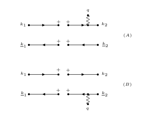
Figure 10: A quark-antiquark pair absorbing or emitting a vector photon in an instanton background labeled by $+$.

$${\rm Fig}.~{}\ref{fig_fr3}A= e_{u}\times\bigg{<}\bigg{(}\bigg{(}u_{R}^{\dagger}(k_{2})(-ik_{2})\epsilon(q)\cdot\overline{V}(q,-k_{2})\bigg{)}\bigg{(}\overline{\phi}(k_{1})(i\overline{k}_{1})u_{L}(k_{1})\bigg{)}\bigg{)}$$

$$\,\,\,\,\,\,\otimes\bigg{(}\big{(}d_{R}^{\dagger}(\underline{k}_{1})(i\underline{k}_{1})K(\underline{k}_{1})\bigg{)}\bigg{(}\overline{\phi}(-\underline{k}_{2})(-i\underline{k}_{2})d_{L}(\underline{k}_{2})\bigg{)}\bigg{)}\bigg{>}_{U}$$

$${\rm Fig}.~{}\ref{fig_fr3}B= e_{\overline{d}}\times\bigg{<}\bigg{(}\bigg{(}u_{R}^{\dagger}(k_{2})(-ik_{2})K(-k_{2})\bigg{)}\bigg{(}\overline{\phi}(k_{1})(i\overline{k}_{1})u_{L}(k_{1})\bigg{)}\bigg{)}$$ (92)

$$\,\,\,\,\,\,\otimes\bigg{(}\big{(}d_{R}^{\dagger}(\underline{k}_{1})(i\underline{k}_{1})K(\underline{k}_{1})\bigg{)}\bigg{(}\epsilon(q)\cdot V(q,-\underline{k}_{2})(-i\overline{\underline{k}}_{2})d_{L}(\underline{k}_{2})\bigg{)}\bigg{>}_{U}$$

where we have now made explicit the different flavors running in the vector vertex in Fig. 10, with the generic notation $u_{\alpha}^{i}(k_{1,2})$ with flavor charge $e_{u}$, and ${d}_{\alpha}^{\dagger i}(\underline{k}_{1,2})$ with flavor charge $e_{\overline{d}}$, and $\alpha=1,2$ for spin and $i=1,..,N_{c}$ for color. Note that we have now attached a color index to each incoming and outgoing quark-antiquark line which is contracted with the pertinent $U$-matrix in the corresponding bracket. To carry the color averaging in (IV.6) we use the identity

$$\int dU\,U^{i}_{\alpha}U^{\dagger\beta}_{j}U^{k}_{\gamma}U^{\dagger\delta}_{l}=\frac{1}{N_{c}^{2}-1}\bigg{(}\delta^{i}_{j}\delta^{k}_{l}\delta^{\beta}_{\alpha}\delta^{\delta}_{\gamma}+\delta^{i}_{l}\delta^{k}_{j}\delta^{\beta}_{\gamma}\delta^{\delta}_{\alpha}\bigg{)}-\frac{1}{N_{c}(N_{c}^{2}-1)}\bigg{(}\delta^{i}_{j}\delta^{k}_{l}\delta^{\beta}_{\gamma}\delta^{\delta}_{\alpha}+\delta^{i}_{l}\delta^{k}_{j}\delta^{\beta}_{\alpha}\delta^{\delta}_{\gamma}\bigg{)}$$ (93)

The result for the symmetrized vector insertion on the quark line in Fig. 10A is

$${\rm Fig}.~{}(\ref{fig_fr3}A+\ref{fig_fr3}\tilde{A})_{I}=i\frac{(2\pi\rho^{\frac{3}{2}})^{4}}{(-iM_{Q}\rho)^{2}}\times e_{u}\times$$

$$\bigg{(}\frac{1}{N_{c}^{2}-1}\bigg{(}u_{R}^{\dagger}(k_{2})(\mathbb{F}_{V}(q,k_{1})+\mathbb{F}_{V}(q,-k_{2}))u_{L}(k_{1})\bigg{)}\bigg{(}d_{R}^{\dagger}(\underline{k}_{1})d_{L}(\underline{k}_{2})\bigg{)}$$

$$+\frac{1}{N_{c}^{2}-1}\bigg{(}u_{R}^{\dagger}(k_{2})(\mathbb{F}_{V}(q,k_{1})+\mathbb{F}_{V}(q,-k_{2}))d_{L}(\underline{k}_{2})\bigg{)}\bigg{(}d_{R}^{\dagger}(\underline{k}_{1})u_{L}(k_{1})\bigg{)}$$

$$-\frac{1}{N_{c}(N_{c}^{2}-1)}\bigg{(}u_{Ri}^{\dagger}(k_{2})(\mathbb{F}_{V}(q,k_{1})+\mathbb{F}_{V}(q,-k_{2}))u^{j}_{L}(k_{1})\bigg{)}\bigg{(}d_{Rj}^{\dagger}(\underline{k}_{1})d^{i}_{L}(\underline{k}_{2})\bigg{)}$$

$$-\frac{1}{N_{c}(N_{c}^{2}-1)}\bigg{(}u_{Ri}^{\dagger}(k_{2})(\mathbb{F}_{V}(q,k_{1})+\mathbb{F}_{V}(q,-k_{2}))d^{j}_{L}(\underline{k}_{2})\bigg{)}\bigg{(}d_{Rj}^{\dagger}(\underline{k}_{1})u^{i}_{L}(k_{1})\bigg{)}\bigg{)}$$

with $M_{Q}$ the constituent quark mass discussed earlier. To avoid cluttering the spin-color indices in the Weyl spinors have been omitted. Each of the L,R-Weyl spinor in the bracket is contracted over the dummy spin $\alpha=1,2$ and color $i=1,...,N_{c}$ indices, unless the contraction is out-of-bracket in which case the pertinent (color) index contraction is displayed. The I-subscript refers to the instanton contribution. The anti-instanton contribution follows from (IV.6) through the substitution $L\leftrightarrow R$. The corresponding result for the symmetrized vector insertion on the anti-quark line in Fig. 10B is

$${\rm Fig}.~{}(\ref{fig_fr3}B+\ref{fig_fr3}\tilde{B})_{I}=i\frac{(2\pi\rho^{\frac{3}{2}})^{4}}{(-iM_{Q}\rho)^{2}}\times e_{\overline{d}}\times$$

$$\bigg{(}\frac{1}{N_{c}^{2}-1}\bigg{(}u_{R}^{\dagger}(k_{2})u_{L}(k_{1})\bigg{)}\bigg{(}d_{R}^{\dagger}(\underline{k}_{1})\mathbb{(}\mathbb{F}_{V}(q,\underline{k}_{1})+\mathbb{F}_{V}(q,-\underline{k}_{2}))d_{L}(\underline{k}_{2})\bigg{)}$$

$$+\frac{1}{N_{c}^{2}-1}\bigg{(}u_{R}^{\dagger}(k_{2})d_{L}(\underline{k}_{2})\bigg{)}\bigg{(}d_{R}^{\dagger}(\underline{k}_{1})\mathbb{(}\mathbb{F}_{V}(q,\underline{k}_{1})+\mathbb{F}_{V}(q,-\underline{k}_{2}))u_{L}(k_{1})\bigg{)}$$

$$-\frac{1}{N_{c}(N_{c}^{2}-1)}\bigg{(}u_{Ri}^{\dagger}(k_{2})u^{j}_{L}(k_{1})\bigg{)}\bigg{(}d_{Rj}^{\dagger}(\underline{k}_{1})\mathbb{(}\mathbb{F}_{V}(q,\underline{k}_{1})+\mathbb{F}_{V}(q,-\underline{k}_{2}))d^{i}_{L}(\underline{k}_{2})\bigg{)}$$

$$-\frac{1}{N_{c}(N_{c}^{2}-1)}\bigg{(}u_{Ri}^{\dagger}(k_{2})d^{j}_{L}(\underline{k}_{2})\bigg{)}\bigg{(}d_{Rj}^{\dagger}(\underline{k}_{1})\mathbb{(}\mathbb{F}_{V}(q,\underline{k}_{1})+\mathbb{F}_{V}(q,-\underline{k}_{2}))u^{i}_{L}(k_{1})\bigg{)}\bigg{)}$$

with the substitution $L\leftrightarrow R$ for the anti-instanton contribution. The spin-valued induced form factor

$$\mathbb{F}_{V}(q,k)=\frac{\epsilon(q)\overline{k}-k\overline{\epsilon}(q)}{2k\cdot q}F(\rho\sqrt{q^{2}})+\bigg{(}\frac{\epsilon(q)(\overline{q}+\overline{k})-(q+k)\overline{\epsilon}(q)}{(k+q)^{2}}-\frac{\epsilon(q)\overline{k}-k\overline{\epsilon}(q)}{2k\cdot q}\bigg{)}F(\rho\sqrt{(k+q)^{2}})$$

simplifies when the quark line is taken on mass-shell ($F(x)=xK_{1}(x)$)

$$\lim_{k^{2}\rightarrow 0}\,\mathbb{F}_{V}(q,k)=\frac{\epsilon(q)\overline{q}-q\overline{\epsilon}(q)}{q^{2}}\,F(\rho\sqrt{q^{2}})=\epsilon_{\mu}(q)q_{\nu}(\sigma^{\mu}\overline{\sigma}^{\nu}-\sigma^{\nu}\overline{\sigma}^{\mu})\frac{1}{q^{2}}\,F(\rho\sqrt{q^{2}})$$ (97)

The full contribution to the hard vector form factor is (IV.6) plus (IV.6) weighted by the instanton averaged density $n/2$, plus the corresponding anti-instanton contribution. The analytically continued result is

$$\epsilon_{\mu}(q)\mathbb{V}^{\mu}(k_{1},k_{2};\underline{k}_{1},\underline{k}_{2};q)=-\frac{8\kappa\pi^{2}}{M_{Q}^{2}}\times$$

$$\bigg{[}e_{u}\times\bigg{\{}\frac{1}{N_{c}^{2}-1}\bigg{(}\overline{u}_{R}(k_{2})\mathbb{(}\mathbb{F}_{V}(q,k_{1})+\mathbb{F}_{V}(q,-k_{2}))u_{L}(k_{1})\bigg{)}\bigg{(}\overline{d}_{R}(\underline{k}_{1})d_{L}(\underline{k}_{2})\bigg{)}$$

$$+\frac{1}{N_{c}^{2}-1}\bigg{(}\overline{u}_{R}(k_{2})\mathbb{(}\mathbb{F}_{V}(q,k_{1})+\mathbb{F}_{V}(q,-k_{2}))d_{L}(\underline{k}_{2})\bigg{)}\bigg{(}\overline{d}_{R}(\underline{k}_{1})u_{L}(k_{1})\bigg{)}$$

$$-\frac{1}{N_{c}(N_{c}^{2}-1)}\bigg{(}\overline{u}_{Ri}(k_{2})\mathbb{(}\mathbb{F}_{V}(q,k_{1})+\mathbb{F}_{V}(q,-k_{2}))u^{j}_{L}(k_{1})\bigg{)}\bigg{(}\overline{d}_{Rj}(\underline{k}_{1})d^{i}_{L}(\underline{k}_{2})\bigg{)}$$

$$-\frac{1}{N_{c}(N_{c}^{2}-1)}\bigg{(}\overline{u}_{Ri}(k_{2})\mathbb{(}\mathbb{F}_{V}(q,k_{1})+\mathbb{F}_{V}(q,-k_{2}))d^{j}_{L}(\underline{k}_{2})\bigg{)}\bigg{(}\overline{d}_{Rj}(\underline{k}_{1})u^{i}_{L}(k_{1})\bigg{)}\bigg{\}}$$

$$+e_{\overline{d}}\times\bigg{\{}\frac{1}{N_{c}^{2}-1}\bigg{(}\overline{u}_{R}(k_{2})u_{L}(k_{1})\bigg{)}\bigg{(}\overline{d}_{R}(\underline{k}_{1})\mathbb{(}\mathbb{F}_{V}(q,\underline{k}_{1})+\mathbb{F}_{V}(q,-\underline{k}_{2}))d_{L}(\underline{k}_{2})\bigg{)}$$

$$+\frac{1}{N_{c}^{2}-1}\bigg{(}\overline{u}_{R}(k_{2})d_{L}(\underline{k}_{2})\bigg{)}\bigg{(}\overline{d}_{R}(\underline{k}_{1})\mathbb{(}\mathbb{F}_{V}(q,\underline{k}_{1})+\mathbb{F}_{V}(q,-\underline{k}_{2}))u_{L}(k_{1})\bigg{)}$$

$$-\frac{1}{N_{c}(N_{c}^{2}-1)}\bigg{(}\overline{u}_{Ri}(k_{2})u^{j}_{L}(k_{1})\bigg{)}\bigg{(}\overline{d}_{Rj}(\underline{k}_{1})\mathbb{(}\mathbb{F}_{V}(q,\underline{k}_{1})+\mathbb{F}_{V}(q,-\underline{k}_{2}))d^{i}_{L}(\underline{k}_{2})\bigg{)}$$

$$-\frac{1}{N_{c}(N_{c}^{2}-1)}\bigg{(}\overline{u}_{Ri}(k_{2})d^{j}_{L}(\underline{k}_{2})\bigg{)}\bigg{(}\overline{d}_{Rj}(\underline{k}_{1})\mathbb{(}\mathbb{F}_{V}(q,\underline{k}_{1})+\mathbb{F}_{V}(q,-\underline{k}_{2}))u^{i}_{L}(k_{1})\bigg{)}\bigg{\}}\bigg{]}+L\leftrightarrow R$$

We dropped a factor of $i$ in switching from the S-matrix to the T-matrix element in the identification of the vector vertex. For the free spinors, we made the substitutions $u_{L,R}^{\dagger}\rightarrow\overline{u}_{L,R}$ and $d_{R,L}^{\dagger}\rightarrow\overline{d}_{R,L}$ when analytically going to Minkowski space as in (155), with the standard Minkowski relation between Dirac and Weyl spinors

$$u=\frac{1+\gamma_{5}}{2}\,u+\frac{1-\gamma_{5}}{2}\,u\equiv u_{R}+u_{L}$$ (99)

and similarly for $d\equiv d_{R}+d_{L}$. More explicitly, the first contribution in (IV.6) due to the instanton can be recast in the form

$$\bigg{(}\frac{N_{c}}{N_{c}^{2}-1}\bigg{)}\bigg{[}e_{u}\mathbb{F}_{P}(\rho\sqrt{-q^{2}})\,{\overline{u}(k_{2}){\frac{i\epsilon_{\mu}(q)\sigma^{\mu\nu}q_{\nu}}{2M_{Q}}\frac{(1-\gamma_{5})}{2}u(k_{1})}}\bigg{]}\bigg{[}\frac{(2\pi\rho)^{2}}{M_{Q}}\overline{d}(\underline{k}_{1})\frac{(1-\gamma_{5})}{2}d(\underline{k}_{2})\bigg{]}$$ (100)

with the spin-valued matrix $\sigma^{\mu\nu}=\frac{i}{2}[\gamma^{\mu},\gamma^{\nu}]$. The first bracket in (100) shows the vector interaction with a chirally flipped u-quark which is purely magnetic. The corresponding Pauli form factor is

$$\mathbb{F}_{P}(\rho\sqrt{-q^{2}})=\frac{8\kappa}{N_{c}}\frac{K_{1}(\rho\sqrt{-q^{2}})}{\rho\sqrt{-q^{2}}}\,$$ (101)

(We again recall that $-q^{2}=Q^{2}>0$.) The second bracket is the chirality flipped d-quark through the instanton zero mode. All contributions in (IV.6) are of this type. (Note that if the amplitude is evaluated at near-zero $Q$, this instanton term contributes to the constituent quark magnetic moment, see Kochelev (2003).)

IV.7 The zero mode contributions to the scalar form factor

This contribution to the hard scalar form factor follows a similar reasoning as in the previous subsection, with two modifications: 1/ in the form factors (IV.6-97) the polarization $\epsilon(q)\rightarrow 1$; 2/ in the contributions (IV.6-IV.6) there is no chirality flip on the leg with the scalar form factor insertion. With this in mind, and making use of the LSZ amputations (E-E) we have

$${\rm Fig}.~{}(\ref{fig_fr3}A+\ref{fig_fr3}\tilde{A})_{S,I}=-i\frac{(2\pi\rho^{\frac{3}{2}})^{4}}{(-iM_{Q}\rho)^{2}}\times\lambda_{u}\times$$

$$\bigg{[}\frac{1}{N_{c}^{2}-1}\bigg{(}u_{L}^{\dagger}(k_{2}){\mathbb{F}}_{S}(q,-k_{2})u_{L}(k_{1})+u_{R}^{\dagger}(k_{2})\overline{\mathbb{F}}_{S}(q,k_{1})u_{R}(k_{1})\bigg{)}\bigg{(}d_{R}^{\dagger}(\underline{k}_{1})d_{L}(\underline{k}_{2})\bigg{)}$$

$$+\frac{1}{N_{c}^{2}-1}\bigg{(}\bigg{(}u_{L}^{\dagger}(k_{2})\mathbb{F}_{S}(q,-k_{2})d_{L}(\underline{k}_{2})\bigg{)}\bigg{(}d_{R}^{\dagger}(\underline{k}_{1})u_{L}(k_{1})\bigg{)}+\bigg{(}d_{R}^{\dagger}(\underline{k}_{1})\overline{\mathbb{F}}_{S}(q,k_{1})u_{R}({k}_{1})\bigg{)}\bigg{(}u_{R}^{\dagger}({k}_{2})d_{L}(\underline{k}_{2})\bigg{)}\bigg{)}$$

$$-\frac{1}{N_{c}(N_{c}^{2}-1)}\bigg{(}\bigg{(}u_{Li}^{\dagger}(k_{2})\mathbb{F}_{S}(q,-k_{2})u^{j}_{L}(\underline{k}_{2})\bigg{)}\bigg{(}d_{Rj}^{\dagger}(\underline{k}_{1})u^{i}_{L}(k_{1})\bigg{)}+\bigg{(}d_{Rj}^{\dagger}(\underline{k}_{1})\overline{\mathbb{F}}_{S}(q,k_{1})u^{i}_{R}({k}_{1})\bigg{)}\bigg{(}u_{Ri}^{\dagger}({k}_{2})d^{j}_{L}(\underline{k}_{2})\bigg{)}\bigg{)}$$

$$-\frac{1}{N_{c}(N_{c}^{2}-1)}\bigg{(}u_{Li}^{\dagger}(k_{2})\overline{\mathbb{F}}_{S}(q,-k_{2})u^{j}_{L}(k_{1})+u_{Ri}^{\dagger}(k_{2})\overline{\mathbb{F}}_{S}(q,k_{1})u^{j}_{R}(k_{1})\bigg{)}\bigg{(}d_{Rj}^{\dagger}(\underline{k}_{1})d^{i}_{L}(\underline{k}_{2})\bigg{)}\bigg{]}$$

with a scalar charge $\lambda_{u}$, and the scalar form factors

$${\mathbb{F}}_{S}(q,-k_{2}) = \frac{\overline{k}_{2}}{M_{Q}^{2}}F(\rho\sqrt{(q+k_{2})^{2}})\rightarrow\frac{\overline{k}_{2}}{M_{Q}^{2}}F(\rho\sqrt{-q^{2}})$$

$${\overline{\mathbb{F}}}_{S}(q,k_{1}) = \frac{{k_{1}}}{M_{Q}^{2}}F(\rho\sqrt{(q-k_{1})^{2}})\rightarrow\frac{{k_{1}}}{M_{Q}^{2}}F(\rho\sqrt{-q^{2}})$$ (103)

The S-subscript refers to the scalar vertex, and the I-subscript referring to the instanton contribution. The anti-instanton contribution follows from (IV.6) through the substitution $L\leftrightarrow R$. The rightmost identity in (IV.7) is the leading contribution in the $k^{2}\rightarrow 0$ limit, with $F(x)=xK_{1}(x)$ after analytical continuation to Minkowski space. The corresponding result for the symmetrized scalar insertion on the anti-quark line in Fig. 10B is

$${\rm Fig}.~{}(\ref{fig_fr3}B+\ref{fig_fr3}\tilde{B})_{S,I}=-i\frac{(2\pi\rho^{\frac{3}{2}})^{4}}{(-iM_{Q}\rho)^{2}}\times\lambda_{\overline{d}}\times$$

$$\bigg{[}\frac{1}{N_{c}^{2}-1}\bigg{(}u_{R}^{\dagger}(k_{2})u_{L}(k_{1})\bigg{)}\bigg{(}\bigg{(}d_{L}^{\dagger}(\underline{k}_{1})\mathbb{F}_{S}(q,-\underline{k}_{2})d_{L}(\underline{k}_{2})\bigg{)}+\bigg{(}d_{R}^{\dagger}(\underline{k}_{1})\overline{\mathbb{F}}_{S}(q,\underline{k}_{1})d_{R}(\underline{k}_{2})\bigg{)}\bigg{)}$$

$$+\frac{1}{N_{c}^{2}-1}\bigg{(}\bigg{(}u_{L}^{\dagger}(k_{2})\mathbb{F}_{S}(q,-\underline{k}_{2})d_{L}(\underline{k}_{2})\bigg{)}\bigg{(}d^{\dagger}_{R}(\underline{k}_{1})u_{L}(k_{1})\bigg{)}+\bigg{(}d^{\dagger}(\underline{k}_{1})\overline{\mathbb{F}}_{S}(q,\underline{k}_{1})u_{L}(k_{1})\bigg{)}\bigg{(}u^{\dagger}_{R}(k_{2})d_{L}(\underline{k}_{2})\bigg{)}\bigg{)}$$

$$-\frac{1}{N_{c}(N_{c}^{2}-1)}\bigg{(}u^{\dagger}_{Li}(k_{2})\mathbb{F}_{S}(q,-\underline{k}_{2})d^{j}_{L}(\underline{k}_{2})\bigg{)}\bigg{(}d^{\dagger}_{Rj}(\underline{k}_{1})u_{L}^{i}(k_{1})\bigg{)}+\bigg{(}d^{\dagger}_{Lj}(\underline{k}_{1})\overline{\mathbb{F}}_{S}(q,\underline{k}_{1})u^{i}_{L}(k_{1})\bigg{)}\bigg{(}u^{\dagger}_{Ri}(k_{2})d_{L}^{j}(\underline{k}_{2})\bigg{)}$$

$$-\frac{1}{N_{c}(N_{c}^{2}-1)}\bigg{(}u^{\dagger}_{Ri}(k_{2})u_{L}^{j}(k_{1})\bigg{)}\bigg{(}d_{Rj}^{\dagger}(\underline{k}_{1})\mathbb{F}_{S}(q,-\underline{k}_{2})d^{i}_{L}(\underline{k}_{2})+d^{\dagger}_{Lj}(\underline{k}_{1})\overline{\mathbb{F}}_{S}(q,\underline{k}_{1})d^{i}_{L}(\underline{k}_{2})\bigg{)}\bigg{]}$$

The anti-instanton contribution follows through the substitution $L\leftrightarrow R$.

The full contribution to the hard scalar form factor is (IV.7) plus (IV.7) weighted again by the instanton averaged density $n/2$, plus the corresponding anti-instanton contribution. The analytically continued result to Minkowski space is

$$\mathbb{S}(k_{1},k_{2};\underline{k}_{1},\underline{k}_{2};q)=+\frac{8\kappa\pi^{2}}{M_{Q}^{2}}\times$$

$$\bigg{[}\lambda_{u}\times\bigg{\{}\frac{1}{N_{c}^{2}-1}\bigg{(}\overline{u}_{L}(k_{2}){\mathbb{F}}_{S}(q,-k_{2})u_{L}(k_{1})+\overline{u}_{R}(k_{2})\overline{\mathbb{F}}_{S}(q,k_{1})u_{R}(k_{1})\bigg{)}\bigg{(}\overline{d}_{R}(\underline{k}_{1})d_{L}(\underline{k}_{2})\bigg{)}$$

$$+\frac{1}{N_{c}^{2}-1}\bigg{(}\bigg{(}\overline{u}_{L}(k_{2})\mathbb{F}_{S}(q,-k_{2})d_{L}(\underline{k}_{2})\bigg{)}\bigg{(}\overline{d}_{R}(\underline{k}_{1})u_{L}(k_{1})\bigg{)}+\bigg{(}\overline{d}_{R}(\underline{k}_{1})\overline{\mathbb{F}}_{S}(q,k_{1})u_{R}({k}_{1})\bigg{)}\bigg{(}\overline{u}_{R}({k}_{2})d_{L}(\underline{k}_{2})\bigg{)}\bigg{)}$$

$$-\frac{1}{N_{c}(N_{c}^{2}-1)}\bigg{(}\bigg{(}\overline{u}_{Li}(k_{2})\mathbb{F}_{S}(q,-k_{2})d^{j}_{L}(\underline{k}_{2})\bigg{)}\bigg{(}\overline{d}_{Rj}(\underline{k}_{1})u^{i}_{L}(k_{1})\bigg{)}+\bigg{(}\overline{d}_{Rj}(\underline{k}_{1})\overline{\mathbb{F}}_{S}(q,k_{1})u^{i}_{R}({k}_{1})\bigg{)}\bigg{(}\overline{u}_{Ri}({k}_{2})d^{j}_{L}(\underline{k}_{2})\bigg{)}\bigg{)}$$

$$-\frac{1}{N_{c}(N_{c}^{2}-1)}\bigg{(}\overline{u}_{Li}(k_{2})\overline{\mathbb{F}}_{S}(q,-k_{2})u^{j}_{L}(k_{1})+\overline{u}_{Ri}(k_{2})\overline{\mathbb{F}}_{S}(q,k_{1})u^{j}_{R}(k_{1})\bigg{)}\bigg{(}\overline{d}_{Rj}(\underline{k}_{1})d^{i}_{L}(\underline{k}_{2})\bigg{)}\bigg{\}}$$

$$+\lambda_{\overline{d}}\times\bigg{\{}\frac{1}{N_{c}^{2}-1}\bigg{(}\overline{u}_{R}(k_{2})u_{L}(k_{1})\bigg{)}\bigg{(}\bigg{(}\overline{d}_{L}(\underline{k}_{1})\mathbb{F}_{S}(q,-\underline{k}_{2})d_{L}(\underline{k}_{2})\bigg{)}+\bigg{(}\overline{d}_{R}(\underline{k}_{1})\overline{\mathbb{F}}_{S}(q,\underline{k}_{1})d_{R}(\underline{k}_{2})\bigg{)}\bigg{)}$$

$$+\frac{1}{N_{c}^{2}-1}\bigg{(}\bigg{(}\overline{u}_{L}(k_{2})\mathbb{F}_{S}(q,-\underline{k}_{2})d_{L}(\underline{k}_{2})\bigg{)}\bigg{(}\overline{d}_{R}(\underline{k}_{1})u_{L}(k_{1})\bigg{)}+\bigg{(}\overline{d}(\underline{k}_{1})\overline{\mathbb{F}}_{S}(q,\underline{k}_{1})u_{L}(k_{1})\bigg{)}\bigg{(}\overline{u}_{R}(k_{2})d_{L}(\underline{k}_{2})\bigg{)}\bigg{)}$$

$$-\frac{1}{N_{c}(N_{c}^{2}-1)}\bigg{(}\overline{u}_{Ri}(k_{2})\mathbb{F}_{S}(q,-\underline{k}_{2})d^{j}_{R}(\underline{k}_{2})\bigg{)}\bigg{(}\overline{d}_{Rj}(\underline{k}_{1})u_{L}^{i}(k_{1})\bigg{)}+\bigg{(}\overline{d}_{Lj}(\underline{k}_{1})\overline{\mathbb{F}}_{S}(q,\underline{k}_{1})u^{i}_{L}(k_{1})\bigg{)}\bigg{(}\overline{u}_{Ri}(k_{2})d_{L}^{j}(\underline{k}_{2})\bigg{)}$$

$$-\frac{1}{N_{c}(N_{c}^{2}-1)}\bigg{(}\overline{u}_{Ri}(k_{2})u_{L}^{j}(k_{1})\bigg{)}\bigg{(}\overline{d}_{Rj}(\underline{k}_{1})\mathbb{F}_{S}(q,-\underline{k}_{2})d^{i}_{R}(\underline{k}_{2})+\overline{d}_{Lj}(\underline{k}_{1})\overline{\mathbb{F}}_{S}(q,\underline{k}_{1})d^{i}_{L}(\underline{k}_{2})\bigg{)}\bigg{\}}\bigg{]}+L\leftrightarrow R$$ (105)

again after dropping a factor of $i$ in going from the S-matrix to the T-matrix element in the identification of the scalar vertex. More explitly, using the limiting form factors (IV.7) the first contribution in (IV.7) can be recast in the compact form

$$\bigg{(}\frac{N_{c}}{N_{c}^{2}-1}\bigg{)}\bigg{[}\lambda_{u}\tilde{\mathbb{F}}_{P}(\rho\sqrt{-q^{2}})\,{\overline{u}(k_{2})\bigg{(}{\frac{k_{+\mu}\gamma^{\mu}+k_{-\mu}\gamma^{\mu}\gamma_{5}}{2M_{Q}}\bigg{)}u(k_{1})}}\bigg{]}\bigg{[}\frac{(2\pi\rho)^{2}}{M_{Q}}\overline{d}(\underline{k}_{1})\frac{(1-\gamma_{5})}{2}d(\underline{k}_{2})\bigg{]}$$ (106)

with $k_{\pm}=(k_{1}\pm k_{2})/2$ (not to be confused with the light cone momenta) and the scalar form factor

$$\tilde{\mathbb{F}}_{P}(x)=\frac{x^{2}\,\mathbb{F}_{P}(x)}{(M_{Q}\rho)^{2}}=\frac{8\kappa}{N_{c}}\frac{F(x)}{(M_{Q}\rho)^{2}}=\frac{8\kappa}{N_{c}}\frac{xK_{1}(x)}{(M_{Q}\rho)^{2}}$$ (107)

Similar reductions hold for the other contractions. In Appendix F we give an alternative but simplified derivation of (106) before analytical continuation and color averaging.

The zero mode instanton plus anti-instanton contribution to the pion vector form factor vanishes for a vanishing tensor DA amplitude $\varphi^{T}_{\pi}(x)=0$,

$$-(e_{u}+e_{\overline{d}})\,\mathbb{F}_{P}(\rho\sqrt{-q^{2}})\,\bigg{(}\frac{N_{c}}{N^{2}_{c}(N_{c}+1)}\bigg{)}\int_{0}^{1}dx_{1}dx_{2}$$

$$\times{\rm Tr}\bigg{[}\bigg{(}\frac{i\epsilon_{\mu}(q)\sigma^{\mu\nu}q_{\nu}}{2M_{Q}}\frac{(1-\gamma_{5})}{2}\bigg{)}\bigg{(}\frac{if_{\pi}}{4}\gamma^{5}(\not{p}\,\varphi_{\pi}(x_{1})-\chi_{\pi}\varphi_{\pi}^{P}(x_{1}))\bigg{)}$$

$$\qquad\times\bigg{(}\frac{(2\pi\rho)^{2}}{M_{Q}}\frac{(1-\gamma_{5})}{2}\bigg{)}\gamma^{0}\bigg{(}\frac{if_{\pi}}{4}\gamma^{5}(\not{p}^{\prime}\,\varphi_{\pi}(x_{2})-\chi_{\pi}\varphi_{\pi}^{P}(x_{2}))\bigg{)}^{\dagger}\gamma^{0}\bigg{]}+{\rm L}\rightarrow{\rm R}=0$$

which is seen to spin trace to zero. The color factor follows directly from the color contraction of (93) in a colorless meson state

$$\frac{\delta^{ik}}{N_{c}}\bigg{[}\bigg{(}\frac{\delta^{i}_{j}\delta^{k}_{l}}{N_{c}^{2}-1}-\frac{\delta^{i}_{l}\delta^{k}_{j}}{N_{c}(N_{c}^{2}-1)}\bigg{)}\delta_{\alpha}^{\beta}\delta_{\gamma}^{\delta}\bigg{]}\frac{\delta^{jl}}{N_{c}}=\frac{\delta_{\alpha}^{\beta}\delta_{\gamma}^{\delta}}{N_{c}^{2}(N_{c}+1)}$$ (109)

The non-vanishing result with the tensor DA amplitude is given in the results section above. Similarly, the zero mode instanton plus anti-instanton contribution to the pion scalar form factor is given by

$$-(\lambda_{u}+\lambda_{\overline{d}})\,\tilde{\mathbb{F}}_{P}(\rho\sqrt{-q^{2}})\,\bigg{(}\frac{N_{c}}{N^{2}_{c}(N_{c}+1)}\bigg{)}\int_{0}^{1}dx_{1}dx_{2}$$

$$\times{\rm Tr}\bigg{[}\bigg{(}\frac{k_{+\mu}\gamma^{\mu}+k_{-\mu}\gamma^{\mu}\gamma_{5}}{2M_{Q}}\bigg{)}\bigg{(}\frac{if_{\pi}}{4}\gamma^{5}\bigg{(}\not{p}\,\varphi_{\pi}(x_{1})-\chi_{\pi}\varphi_{\pi}^{P}(x_{1})+i\chi_{\pi}\sigma_{\alpha\beta}\frac{p^{\alpha}p^{\prime\beta}}{p\cdot p^{\prime}}\frac{\varphi_{\pi}^{T\prime}(x_{1})}{6}\bigg{)}\bigg{)}$$

$$\times\bigg{(}\frac{(2\pi\rho)^{2}}{M_{Q}}\frac{(1-\gamma_{5})}{2}\bigg{)}\gamma^{0}\bigg{(}\frac{if_{\pi}}{4}\gamma^{5}\bigg{(}\not{p}^{\prime}\,\varphi_{\pi}(x_{2})-\chi_{\pi}\varphi_{\pi}^{P}(x_{2})+i\chi_{\pi}\sigma_{\alpha\beta}\frac{p^{\prime\alpha}p^{\beta}}{p\cdot p^{\prime}}\frac{\varphi_{\pi}^{T\prime}(x_{2})}{6}\bigg{)}\bigg{)}^{\dagger}\gamma^{0}\bigg{]}$$

$$+{\rm L}\rightarrow{\rm R}$$ (110)

with the result of all tracing given in the results section above.

IV.8 The zero mode contribution to the graviton and dilaton
form factor of the pion

The mixed zero-mode and non-zero mode contribution (^′t Hooft vertex) follows from (IV.6) with (100) now reading

$$\bigg{(}\frac{N_{c}}{N_{c}^{2}-1}\bigg{)}\bigg{[}\mathbb{F}_{P}(Q\rho)\,{\overline{u}(k_{2}){\frac{i(k_{1}+k_{2})^{[\mu}\sigma^{\nu]_{+}\tau}q_{\tau}}{2M_{Q}}\frac{(1-\gamma_{5})}{2}u(k_{1})}}\bigg{]}\bigg{[}\frac{(2\pi\rho)^{2}}{M_{Q}}\overline{d}(\underline{k}_{1})\frac{(1-\gamma_{5})}{2}d(\underline{k}_{2})\bigg{]}$$ (111)

The mixed-zero mode and non-zero mode vertex (111) contributes equally to $00$ and $\mu\mu$ in the Breit frame, with the result

$$T^{\pi}_{00d}(Q^{2})=T^{\pi}_{\mu\mu d}(Q^{2})=\frac{1}{N_{c}^{2}(N_{c}+1)}\bigg{(}\frac{16\kappa\pi^{2}f_{\pi}^{2}\chi_{\pi}^{2}}{3M_{Q}^{2}}\bigg{)}\left<(Q\rho)K_{1}(Q\rho)\right>\int dx_{1}dx_{2}\,\varphi_{\pi}(x_{1})\frac{\varphi_{\pi}^{T\prime}(x_{2})}{6}$$ (112)

which is seen to vanish.

IV.9 The zero mode contribution to the transverse rho form factors

The instanton plus anti-instanton contribution to the transversely polarized vector form factor is

$$V_{d}^{\rho}(Q^{2})=-(e_{u}+e_{\overline{d}})\,\mathbb{F}_{P}(\rho Q)\,\bigg{(}\frac{N_{c}}{N_{c}^{2}(N_{c}+1)}\bigg{)}\int_{0}^{1}dx_{1}dx_{2}$$

$$\times{\rm Tr}\bigg{[}\bigg{(}\frac{i\sigma^{\mu\nu}q_{\nu}}{2M_{Q}}\frac{(1-\gamma_{5})}{2}\bigg{)}\bigg{(}\frac{i}{4}\not{\epsilon}_{T}\bigg{(}f_{\rho}m_{\rho}\varphi_{\rho}(x_{1})-f_{\rho}^{T}\not{p}\varphi_{\rho}^{T}(x_{1})\bigg{)}+\frac{f_{\rho}m_{\rho}}{4p\cdot p^{\prime}}\epsilon_{\mu\nu\rho\sigma}\gamma^{\mu}\gamma_{5}\epsilon^{\nu}p^{\rho}p^{\prime\sigma}\frac{\varphi_{\rho}^{A\prime}(x_{1})}{4}\bigg{)}$$

$$\times\bigg{(}\frac{(2\pi\rho)^{2}}{M_{Q}}\frac{(1-\gamma_{5})}{2}\bigg{)}\gamma^{0}\bigg{(}\frac{i}{4}\not{\epsilon}_{T}\bigg{(}f_{\rho}m_{\rho}\varphi_{\rho}(x_{2})-f_{\rho}^{T}\not{p}^{\prime}\varphi_{\rho}^{T}(x_{2})\bigg{)}+\frac{f_{\rho}m_{\rho}}{4p\cdot p^{\prime}}\epsilon_{\mu\nu\rho\sigma}\gamma^{\mu}\gamma_{5}\epsilon^{\nu}p^{\prime\rho}p^{\sigma}\frac{\varphi_{\rho}^{A\prime}(x_{2})}{4}\bigg{)}^{\dagger}\gamma^{0}$$

$$+{\rm L}\rightarrow{\rm R}$$

$$=(e_{u}+e_{\overline{d}})\,\mathbb{F}_{P}(\rho\sqrt{-q^{2}})\,\bigg{(}\frac{N_{c}}{N_{c}^{2}(N_{c}+1)}\bigg{)}$$

$$\times{\rm Tr}\bigg{[}\bigg{(}\frac{i\sigma^{\mu\nu}q_{\nu}}{2M_{Q}}\bigg{)}\bigg{(}+\frac{i}{4}{f^{T}_{\rho}}\not{p}\,\not{\epsilon}_{T}\bigg{)}\left(\frac{(2\pi\rho)^{2}}{M_{Q}}\right)\bigg{(}-\frac{i}{4}\not{\epsilon}^{\prime*}_{T}\,{f^{T}_{\rho}}\not{p}^{\prime}\bigg{)}\bigg{]}$$

Unwinding the last trace gives

$$V_{d}^{\rho}(Q^{2})=-(e_{u}+e_{\overline{d}})\bigg{(}(p^{\mu}+p^{\prime\mu})\,\epsilon_{T}^{\prime*}\cdot\epsilon_{T}\bigg{)}\,\bigg{[}\left<(\rho Q)\,{K_{1}(\rho Q)}\right>\,\bigg{(}\frac{2\kappa\pi^{2}}{N_{c}^{2}(N_{c}+1)}\frac{{\tilde{f}_{\rho}}^{2}}{M^{2}_{Q}}\bigg{)}\bigg{]}$$ (114)

which is to be compared to the hard perturbative contribution (55). The instanton plus anti-instanton contribution to the transversely polarized rho scalar form factor is given by

$$S_{d}^{\rho}(Q^{2})=-(\lambda_{u}+\lambda_{\overline{d}})\,\tilde{\mathbb{F}}_{P}(\rho Q)\,\bigg{(}\frac{N_{c}}{N_{c}^{2}(N_{c}+1)}\bigg{)}\int_{0}^{1}dx_{1}dx_{2}$$

$$\times{\rm Tr}\bigg{[}\bigg{(}\frac{k_{+\mu}\gamma^{\mu}+k_{-\mu}\gamma^{\mu}\gamma_{5}}{2M_{Q}}\bigg{)}\bigg{(}\frac{i}{4}\not{\epsilon}_{\perp}\bigg{(}f_{\rho}m_{\rho}\varphi_{\rho}(x_{1})-f_{\rho}^{T}\not{p}\varphi_{\rho}^{T}(x_{1})\bigg{)}+\frac{f_{\rho}m_{\rho}}{4p\cdot p^{\prime}}\epsilon_{\mu\nu\rho\sigma}\gamma^{\mu}\gamma_{5}\epsilon^{\nu}p^{\rho}p^{\prime\sigma}\frac{\varphi_{\rho}^{A\prime}(x_{1})}{4}\bigg{)}$$

$$\times\frac{(2\pi\rho)^{2}}{M_{Q}}\bigg{(}\frac{(1-\gamma_{5})}{2}\bigg{)}\gamma^{0}\bigg{(}\frac{i}{4}\not{\epsilon}_{\perp}\bigg{(}f_{\rho}m_{\rho}\varphi_{\rho}(x_{2})-f_{\rho}^{T}\not{p}\varphi_{\rho}^{T}(x_{2})\bigg{)}+\frac{f_{\rho}m_{\rho}}{4p\cdot p^{\prime}}\epsilon_{\mu\nu\rho\sigma}\gamma^{\mu}\gamma_{5}\epsilon^{\nu}p^{\prime\rho}p^{\sigma}\frac{\varphi_{\rho}^{A\prime}(x_{2})}{4}\bigg{)}^{\dagger}\gamma^{0}\bigg{]}$$

$$+{\rm L}\rightarrow{\rm R}$$ (115)

with the full tracing result given in the results section above.

IV.10 Averaging over the instanton size distribution

In the expressions above and for simplicity, we have used a single value of the instanton size $\rho$. For many estimates it is sufficient to use its r.m.s. value of about $0.30\,{\rm fm}$. Yet in cases in which a large momentum transfer is involved, the shape of the distribution over $\rho$ becomes important, especially its tail toward small sizes. Fortunately, at small $\rho$ the effective coupling $\alpha_{s}(\rho)$ is small, the action is large and semiclassical theory get more reliable.

Still, one needs the full shape of the distribution, to get a proper averaging. The instanton size distribution in the QCD vacuum has been derived from lattice works, using various degree of “cooling” methods, e.g. Hasenfratz (2000). We will not dwell on the details of this distribution, and we will not get involved in the theoretical aspects of the large large-size instantons for which we refer to e.g. ref.Shuryak (1999). Here we make use of the interpolating formula

$$dn(\rho)\sim{d\rho\over\rho^{5}}\big{(}\rho\Lambda_{QCD}\big{)}^{b_{QCD}}\,e^{-2\pi\sigma\rho^{2}}$$ (116)

in which the pre-exponential is the semi-classical contribution corrected to one-loop with $b_{QCD}=11N_{c}/3-2N_{f}/3\approx 9$. The exponent is model-dependent, with $\sigma$ the QCD string tension. (It is proportional to the dual magnetic condensate, that of Bose-condensed monopoles, but we prefer the expression with the string tension which is experimentally well determined to be $\sigma\approx 0.42\,{\rm GeV}^{2}$.)

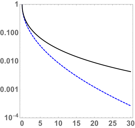
Figure 11: The blue dashed line is the exponential function $e^{-Q\rho_{r.m.s.}}$ of momentum transfer $Q$, and the solid line is the same function averaged over the instanton size distribution, plotted versus $Q^{2}\,({\rm GeV}^{2})$.

In Fig.11 we show the effect of averaging over the instanton size distribution. We take a simple typical exponential dependence on the momentum transfer, and compare it to its version after the instanton size averaging

$$\langle e^{-Q\rho}\rangle_{\rho}={\int dn(\rho)\,e^{-Q\rho}\over\int dn(\rho)}$$ (117)

As one can see, at small $Q$ the two curves coincide, but at large $Q$ they differ significantly. The small-size instantons become more important in this limit, and the exponential decay with $Q$ changes to an inverse power.

All of the Bessel functions $K_{i}(Q\rho)$ appearing above in the instanton-induced form factors behave as $\sim e^{-Q\rho}$ at large $Q$, so the result of their averaging over the instanton sizes is similar to what is shown in Fig.11. Yet, when we performed the instanton size averaging of the functions $F_{1,2}$, as given in (LABEL:eqn_F2), we found that their corrections due to averaging differ substantially, resulting in significant changes in the outcome.

V Mesonic light-front distribution amplitudes

V.1 Brief history of mesonic DA’s and exclusive processes

In the pioneering works on theory of exclusive QCD processes Chernyak and Zhitnitsky (1977); Lepage and Brodsky (1979); Efremov and Radyushkin (1980), most of the general structure and observations were made. The key element of the theory is the $factorization$ into a hard block and a light-front DA’s, with the latter containing most of the information about the soft physics at a scale much below the hard scale $Q^{2}$.

The DA’s are defined as the hadron wave function integrated over the transverse momentum. They are traditionally defined via bilocal light cone operators, classified in the framework of a twist expansion, the leading twist 2, and higher, with extra powers of $1/Q$. Twist is spin minus dimension. This theory originated from DIS in which moments of PDFs are matrix elements of the leading twist operators, containing only bilinear quark (or gluon) fields. Higher twist operators, specified for unpolarized and polarized DIS in Shuryak and Vainshtein (1982a, b), contain important further information about the nucleon structure, such as correlations between quark and gluon fields, or quark-quark correlation via four-fermion operators.

However, unlike in DIS, the exclusive processes are studied at what we call a “semi-hard” domain, in which one cannot expect the twist expansion to converge. In particular, as pointed out early on by Geshkenbein and Terent’ev Geshkenbein and Terentev (1982), the twist-3 DA’s of the pion are numerically enhanced, so that their contribution may in fact be larger than that of the leading twist, in the semi-hard $Q^{2}$ range of interest.

Even more academic is the discussion of the asymptotic limit, in which not powers of $Q^{2}$, but powers of log are considered to be large, i.e. ${\rm log}(Q^{2}/\Lambda_{QCD}^{2})\gg 1$. When perturbative processes of gluon radiation are included, these logs sum into calculable anomalous dimension of various operators. So when the log is considered to be large, only the leading contribution survives.

Technically, the DA’s are decomposed into Gegenbauer polynomials, and the so called “asymptotic wave function” corresponds to the lowest order polynomial.

$$\varphi_{\pi}\rightarrow\varphi^{\rm asymptotic}_{\pi}(\xi)=\frac{3}{4}(1-\xi^{2})=6x\bar{x}$$ (118)

Needless to say, this limit is very far from the realistic kinematic range of interest. Therefore we will neither use “asymptotic wave functions”, nor restrict our analysis to the leading twist DA’s. We rather focus on the chiral structure of the DA’s, making sure that all possible and large contributions are included. For phenomenological purposes it is sufficient to consider a set of DA’s approximated by the simple analytic form

$$\varphi_{\pi}(\xi,p)={\Gamma(3/2+p)\over\sqrt{\pi}\Gamma(1+p)}(1-\xi^{2})^{p}={6^{p}\Gamma(3/2+p)\over\sqrt{\pi}\Gamma(1+p)}\,(x\bar{x})^{p}$$ (119)

The case $p=1$ is the “asymptotic” distribution, while the case $p=0$ is called “flat”. Several authors have used an intermediate case $p=1/2$ called “semicircular”.

The pion is a particular particle, a Nambu-Goldstone mode, and therefore its properties one can calculate in any theory in which chiral symmetry gets spontaneously broken. Historically the NJL model and its nonlocal versions (some related with the instanton liquid model) have been used to calculate the pion light-front wave function Broniowski and Ruiz Arriola (2017); Petrov and Pobylitsa (1997); Anikin et al. (2001). Before we briefly discuss the results of “realistic” models, related to larger set of hadronic wave functions, let us introduce some extreme cases. For example, in Ruiz Arriola and Broniowski (2002) a “flat” pion wave function was used as an “initial condition” for radiative evolution. Some typical shapes of the pion and other light meson wave functions stemming from some recent works, are shown in Fig.12.

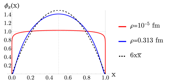
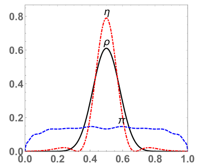
Figure 12: Upper plot: the pion light front distribution function from Kock et al. (2020). Lower plot: the light meson light front distribution functions from Shuryak (2019).

In contrast, in 1980’s Chernyak and collaborators Chernyak and Zhitnitsky (1984), using the QCD sum rules, arrived at the pion wave function

$$\varphi_{CZ}(x)=30x(1-x)(2x-1)^{2}$$ (120)

known as “the double-hump” one. But, since then no support for this shape has materialized, and it also does not agree with lattice results on momentum fractions, so we will not discuss it. Let us state once again, that we see phenomenological failure of the pQCD expressions not in the modified shape of the wave function, but in missing nonperturbative part of the hard blocks.

The light pseudoscalar mesons $P=\pi,K,\eta$ are related to chiral symmetry breaking and therefore they exist even in models without confinement, such as the NJL and ILM. Their wave functions and parton distribution amplitudes (PDA) have been calculated in various approximations. The question was addressed originally in the ILM framework in Petrov et al. (1999), and more recently using the quasi-distribution proposal by one of us in Kock et al. (2020). The distribution amplitude for the light P-pseudoscalars of squared mass $m_{P}^{2}$ was derived in Kock et al. (2020)

$$\varphi_{P}(x)=\frac{2N_{c}}{f^{2}_{P}}\int\frac{d^{2}k_{\perp}}{(2\pi)^{3}}\frac{\theta(x\bar{x})}{(k_{\perp}^{2}+M^{2}(0,m_{q})-x\bar{x}m_{P}^{2})}\,M^{2}\bigg{(}\frac{\sqrt{k^{2}_{\perp}+M^{2}(0,m_{q})}}{\lambda_{P}\sqrt{x\bar{x}}}\bigg{)}$$ (121)

where the momentum-dependent quark mass is

$$M(k,0)=M(0)\bigg{(}\bigg{|}z\bigg{(}I_{0}K_{0}-I_{1}K_{1}\bigg{)}^{\prime}\bigg{|}^{2}\bigg{)}_{z=\frac{1}{2}\rho k}$$ (122)

Here $\lambda_{P}$ is a cut-off parameter of order 1, e.g. $\lambda_{\pi}=3.41$, and $M(0)=386\,{\rm MeV}\approx M_{Q}$ with an instanton size $\rho=0.3$ fm. As shown in Kock et al. (2020), this momentum dependence has been confirmed by lattice studies. For a light current quark mass $m_{q}$, the running effective quark mass $M(k,m_{q})\approx M(k)+m_{q}$. The corresponding shape of the wave function is shown in the upper plot of Fig.12 as reproduced from Kock et al. (2020), is in agreement with Petrov et al. (1999). Both calculations show a wave functions rather close to the asymptotic one, and very far from the “double-hump” distribution (120).

Another approach to light front wave functions is based on some model-dependent Hamiltonians. Jia and Vary Jia and Vary (2019) introduced a convenient form of it, with three basic elements: constituent quark masses (that is, chiral symmetry breaking), plus some form of confinement, plus (NJL-type) residual quark-quark interaction. This approach was followed by one of us Shuryak (2019), who calculated the wave functions for the $\pi,\rho,\eta^{\prime}$ mesons, as shown in the lower plot of Fig.12.

We do not study or discuss in this work other hadrons, such as baryons, pentaquarks and dibaryons, or multi-quark components of meson wave functions. Still, let us make here few remarks on those. Their PDF’s, extracted from DIS and jets, are in this case not sufficient to obtain the wave functions and DA’s, as they depend on more variables. And yet, it is very important to study those: in particular, the structure of the nucleons is the central area of experimental research. So, let us mention few works on that related with instanton effects.

In 1990’s Diakonov and collaborators have developed a version of the chiral bag model based on the ILM, and calculated certain leading and next-to-leading twist nucleons DA’s, for a review see Polyakov and Weiss (1997). Unfortunately, it was done in the large $N_{c}$ limit, which missed important elements, such as the instanton-induced diquarks Rapp et al. (1998). The wave functions for the $\Delta$, the nucleon and even their 5-light-quark component were derived recently in Shuryak (2019), with the t’Hooft residual interaction. It provides the first quantitative derivation of the $anti$quark PDFs inside the nucleon, explaining its flavor asymmetry.

V.2 Twist and chiral structures of the DA’s of the pion

We start this section from a generic discussion of chiral symmetry and its breaking. Naively, in a theory with $massless$ quarks chiral symmetry is exact. If it remains unbroken, hadrons diagonal in chirality such as $\overline{q}_{L}q_{L}+\overline{q}_{R}q_{R}$, and non-diagonal in chirality such as $\overline{q}_{L}q_{R}+\overline{q}_{R}q_{L}$ would simply be different species, with different masses and wave functions. Since chiral symmetry is spontaneously broken in the QCD vacuum (and at low temperatures $T<T_{c}$), all such would be species are mixed together.

Starting from the QCD sum rule days of 1970’s, it is known that hadrons can be excited by local operators with different chiral structure. For example, positive pions can be excited $both$ by (chiral non-diagonal) pseudoscalar operator $(\bar{d}i\gamma_{5}u)$ and (diagonal) axial current $(\bar{d}\gamma_{\mu}\gamma_{5}u)$. Yet the pion role in these two correlation functions is very different. While in the pseudoscalar correlator the pion practically dominates from very small distances on, in the axial-vector correlator the $A_{1}$ meson dominates, and only at rather large distances a pion tail appears. The coupling to the axial-vector current $f_{\pi}$, is relatively small, and vanishes if chiral symmetry is restored.

In the case of the pion, the DA is $\pi^{+}(p)\rightarrow q_{if\alpha}(k)\bar{q}_{jg\beta}(k-p)$ corresponds formally to the connected amplitude

$$\int_{-\infty}^{+\infty}\frac{p^{+}dz^{-}}{2\pi}e^{ixp\cdot z}\left<0\left|\overline{d}_{\beta}(0)[0,z]u_{\alpha}(z)\right|\pi^{+}(p)\right>$$

$$=\bigg{(}+\frac{if_{\pi}}{4}\gamma^{5}\bigg{(}\not{p}\,\varphi_{\pi^{+}}(x)-\chi_{\pi}\varphi_{\pi}^{P}(x)+i\chi_{\pi}\sigma_{\alpha\beta}\frac{p^{\alpha}p^{\prime\beta}}{p\cdot p^{\prime}}{\varphi_{\pi}^{\prime\,T}(x)\over{6}}\bigg{)}\bigg{)}_{\alpha\beta}$$ (123)

and its conjugate

$$\int_{-\infty}^{+\infty}\frac{p^{\prime-}dz^{+}}{2\pi}e^{-ixp^{\prime}\cdot z}\left<\pi^{+}(p^{\prime})\left|\overline{u}_{\beta}(z)[z,0]d_{\alpha}(0)\right|0\right>$$

$$=\bigg{(}-\frac{if_{\pi}}{4}\gamma^{5}\bigg{(}\not{p}^{\prime}\,\varphi_{\pi^{+}}(x)+\chi_{\pi}\varphi_{\pi}^{P}(x)-i\chi_{\pi}\sigma_{\alpha\beta}\frac{p^{\alpha}p^{\prime\beta}}{p\cdot p^{\prime}}{\varphi_{\pi}^{\prime\,T}(x)\over{6}}\bigg{)}\bigg{)}_{\alpha\beta}$$ (124)

up to twist-3. $[x,y]$ refers to the gauge link and $\sigma_{\alpha\beta}=\frac{i}{2}[\gamma_{\alpha},\gamma_{\beta}]$. (V.3-V.3) are explicitly odd under P parity.

Note that the 4-vector $p^{\prime}_{\mu}$ appears in the DA of a pion with 4-vector $p_{\mu}$, in reference to the conjugate light-cone direction, with generally no relation to the second pion. In the DA of a pion with momentum $p^{\prime}_{\mu}$, the exchange $p\leftrightarrow p^{\prime}$ needs to be enforced, effectively flipping the sign of the last term. Also, note that we dropped the contribution

$$\frac{f_{\pi}\chi_{\pi}}{4}\sigma_{\mu\nu}p^{\mu}\bigg{[}\bigg{(}\frac{\partial}{\partial k_{\perp\nu}}\frac{\varphi_{\pi}^{T}(x)}{6}\bigg{)}+\frac{\varphi_{\pi}^{T}(x)}{6}\frac{\partial}{\partial k_{\perp\nu}}\bigg{]}$$ (125)

as it involves the dependence on $k_{\perp}$ which we have ignored in both the soft and hard blocks.

(V.3-V.4) can be inverted, to recast the pion twist-2 and twist-3 light-cone wavefunctions in explicit form

$$\varphi_{\pi^{+}}(x)=\frac{1}{if_{\pi}}\int_{-\infty}^{+\infty}\frac{dz^{-}}{2\pi}e^{ixp\cdot z}\left<0\left|\overline{d}(0)\gamma^{+}\gamma_{5}[0,z]u(z)\right|\pi^{+}(p)\right>$$

$$\varphi^{P}_{\pi^{+}}(x)=\frac{p^{+}}{f_{\pi}\chi_{\pi}}\int_{-\infty}^{+\infty}\frac{dz^{-}}{2\pi}e^{ixp\cdot z}\left<0\left|\overline{d}(0)i\gamma_{5}[0,z]u(z)\right|\pi^{+}(p)\right>$$

$$\frac{\varphi^{T\prime}_{\pi^{+}}(x)}{6}=\frac{1}{f_{\pi}\chi_{\pi}}\frac{p^{\mu}p^{\prime\nu}p^{+}}{p\cdot p^{\prime}}\int_{-\infty}^{+\infty}\frac{dz^{-}}{2\pi}e^{ixp\cdot z}\left<0\left|\overline{d}(0)\sigma_{\mu\nu}\gamma_{5}[0,z]u(z)\right|\pi^{+}(p)\right>$$ (126)

with all DA normalized to 1. The leading twist-2 DA $\varphi_{\pi}(x)$ is chirally-diagonal. Although it characterizes the axial-vector strength in the pion, it is traditionally referred to without the label $A$ or axial, a convention we will hold. Its normalization to 1 is fixed by the weak pion decay constant $f_{\pi}\approx 133\,{\rm MeV}$,

$$\left<0\left|\overline{d}(0)\gamma^{\mu}{(1-\gamma^{5})}u(0)\right|\pi^{+}(p)\right>=-{\rm Tr}\bigg{(}\gamma^{\mu}{(1-\gamma^{5})}\bigg{(}\frac{if_{\pi}}{4}\gamma^{5}\not{p}\bigg{)}\bigg{)}\,\int_{0}^{1}dx\,\varphi_{\pi^{+}}(x)\equiv if_{\pi}\,p^{\mu}$$ (127)

Isospin symmetry and charge conjugation force $\varphi_{\pi}(x)=\varphi_{\pi}(\overline{x})$. As pointed out initially in Geshkenbein and Terentev (1982), there are two twist-3 and chirally non-diagonal independent DA $\varphi^{P}_{\pi}(x)$ and $\varphi_{\pi}^{T}(x)$, characterizing the pseudoscalar and tensor strength in the pion respectively. The latters are tied by the current identity

$$\partial^{\nu}\big{(}\overline{d}(0)\sigma_{\mu\nu}\gamma_{5}u(z)\big{)}=-\partial_{\mu}\big{(}\overline{d}(0)i\gamma_{5}u(z)\big{)}+m\,\overline{d}(0)\gamma_{\mu}\gamma_{5}u(z)$$ (128)

and share the same couplings. The value of the dimensionful coupling constant $\chi_{\pi}$ can be fixed by the divergence of the axial-vector current and the PCAC relation

$$(m_{u}+m_{d})\left<0\left|\overline{d}(0)i\gamma^{5}u(0)\right|\pi^{+}(p)\right>=$$

$$-(m_{u}+m_{d})\,{\rm Tr}\bigg{(}i\gamma^{5}\bigg{(}\frac{if_{\pi}}{4}\gamma^{5}\chi_{\pi}\bigg{)}\bigg{)}\,\int_{0}^{1}dx\,\varphi_{\pi}^{P}(x)=(m_{u}+m_{d})\,f_{\pi}\chi_{\pi}$$ (129)

with $\varphi_{\pi}^{P}(x)$ normalized to 1. Using the Gell-Mann-Oakes-Renner relation

$$f_{\pi}^{2}m_{\pi}^{2}=-2(m_{u}+m_{d})\left<\overline{q}q\right>$$ (130)

with $|\left<\overline{q}q\right>|\approx(240\,{\rm MeV})^{3}$, which yields

$$\chi_{\pi}=\frac{m_{\pi}^{2}}{(m_{u}+m_{d})}$$ (131)

Furthermore, quark masses are not physical quantities and their numerical values depend on the definition, in particular on chosen normalization point $\mu$. PDG tables use rather high value $\mu=2\,GeV$, appropriate e.g. to lattice simulations with fine lattices. For usage in DA’s more appropriate are values at “soft” normalization, as used in hadronic spectroscopy, which are about twice larger than PDG values. Therefore we will use for $\chi_{\pi}\approx 1.2\,GeV$.

Note that while the coupling to the pseudoscalar current is numerically large compared to $f_{\pi}$, this term flips the quark chirality. For the vector form factor, this term contributes typically subleading corrections $\sim\chi_{\pi}^{2}/Q^{2}$. However, as we have shown in our summary results, its contribution is far from being negligible in the kinematical region of interest.

Asymptotically, twist-3 contributions combined together give subleading contributions to the pion form factor at large $Q^{2}$ as can be seen in (II.1). Indeed, the asymptotic limits of these DA’s are $\varphi_{\pi}^{P}(x)\rightarrow 1$ and $\varphi_{T}(x)\rightarrow 6x\bar{x}$ owing to their conformal spin, with $\varphi_{T}^{\prime}(x)\rightarrow 6(\bar{x}-x)$. When inserted in (II.1) the twist-3 contribution simplifies at asymptotic $Q$ with the result

$$\frac{f_{\pi}^{2}\chi_{\pi}^{2}}{Q^{4}}\int dx_{1}dx_{2}\,{1\over\bar{x}_{1}\bar{x}_{2}}\bigg{[}\bigg{(}\frac{1}{\bar{x}_{2}}-1\bigg{)}+(\bar{x}_{2}-x_{2})\bigg{(}\frac{1}{\bar{x}_{2}}+1\bigg{)}=2\bar{x}_{2}\bigg{]}=2\frac{f_{\pi}^{2}\chi_{\pi}^{2}}{Q^{4}}\int\frac{dx_{1}}{\bar{x}_{1}}\,\,$$ (132)

which is clearly subleading. However, in the semi-hard domain of interest for this work, one does not expect the twist expansion to converge. Moreover, as was also noted already in Geshkenbein and Terentev (1982), while suppressed asymptotically, P and T contributions are actually enhanced by a large prefactor, and are in fact dominant over the leading axial term.

V.3 The twist and chiral structure of DA’s
of the transversely polarized vector mesons

The DA’s of the vector mesons, with longitudinal and transverse polarizations, are extensively discussed in the literature. We refer to Ball and Braun (1996, 1998) for a thorough discussion of the leading and subleading twist contributions, and how their couplings are related. We will mostly discuss the transversely polarized $\rho^{+}$, with the following twist-2 and twist-3 DA

$$\varphi_{\rho_{\perp}}(x)= g_{\perp}^{(v)}(x)=\frac{p^{+}}{f_{\rho}m_{\rho}}\int_{-\infty}^{+\infty}\frac{dz^{-}}{2\pi}e^{ixp\cdot z}\,\left<0\left|\overline{d}(0)\not{\epsilon}_{\perp}u(z)\right|\rho^{+}(p)\right>$$

$$\varphi^{T}_{\rho_{\perp}}(x)= \phi_{\perp}(x)=\frac{p^{+}}{2f^{T}_{\rho}p\cdot p^{\prime}}\int_{-\infty}^{+\infty}\frac{dz^{-}}{2\pi}e^{ixp\cdot z}\left<0\left|\overline{d}(0)(\not{\epsilon}_{\perp}\not{p}^{\prime}-\epsilon_{\perp}\cdot p)u(z)\right|\rho^{+}(p)\right>$$

$$\varphi^{\prime\,A}_{\rho_{\perp}}(x)= g_{\perp}^{\prime\,(a)}(x)=\frac{2ip^{+}}{3f_{\rho}m_{\rho}p\cdot p^{\prime}}\epsilon^{\mu\nu\rho\sigma}{\epsilon_{T\mu}}p^{\prime}_{\rho}p_{\sigma}\int_{-\infty}^{+\infty}\frac{dz^{-}}{2\pi}e^{ixp\cdot z}\,\left<0\left|\overline{d}(0)\gamma_{\mu}\gamma_{5}u(z)\right|\rho^{+}(p)\right>$$

with non-vanishing $\epsilon^{\mu}_{\perp}\neq 0$ only for $\mu=1,2$. The first labeling refers to our notations, and the second labeling to the notations used in Ball and Braun (1996).

Expressions (V.3) can be inverted, to give the transverse rho twist-2 and twist-3 light-cone wavefunctions in explicit form

$$\int_{-\infty}^{+\infty}\frac{p^{+}dz^{-}}{2\pi}e^{ixp\cdot z}\left<0\left|\overline{d}_{\beta}(0)[0,z]u_{\alpha}(z)\right|\rho^{+}(p)\right>$$

$$=\bigg{(}+\frac{i}{4}\not{\epsilon}_{\perp}\bigg{(}f_{\rho}m_{\rho}\varphi_{\rho}(x)-f_{\rho}^{T}\not{p}\varphi_{\rho}^{T}(x)\bigg{)}+\frac{f_{\rho}m_{\rho}}{4p\cdot p^{\prime}}\epsilon_{\mu\nu\rho\sigma}\gamma^{\mu}\gamma_{5}\epsilon^{\nu}p^{\rho}p^{\prime\sigma}\frac{\varphi_{\rho}^{A\prime}(x)}{4}\bigg{)}_{\alpha\beta}$$ (134)

and its conjugate

$$\int_{-\infty}^{+\infty}\frac{p^{\prime-}dz^{+}}{2\pi}e^{-ixp^{\prime}\cdot z}\left<\rho^{+}(p^{\prime})\left|\overline{u}_{\beta}(z)[z,0]d_{\alpha}(0)\right|0\right>$$

$$=\bigg{(}-\frac{i}{4}\not{\epsilon}_{\perp}\bigg{(}f_{\rho}m_{\rho}\varphi_{\rho}(x)+f_{\rho}^{T}\not{p}^{\prime}\varphi_{\rho}^{T}(x)\bigg{)}-\frac{f_{\rho}m_{\rho}}{4p\cdot p^{\prime}}\epsilon_{\mu\nu\rho\sigma}\gamma^{\mu}\gamma_{5}\epsilon^{\nu}p^{\rho}p^{\prime\sigma}\frac{\varphi_{\rho}^{A\prime}(x)}{4}\bigg{)}_{\alpha\beta}$$ (135)

with again all DA normalized to 1. The parameter $f_{\rho}\approx 210\,{\rm MeV}$ is fixed from the electromagnetic decay $\rho\rightarrow e^{+}e^{-}$,

$$\left<0\left|\overline{d}(0)\gamma^{\mu}u(0)\right|\rho_{\perp}^{+}(p)\right>=-\int_{0}^{1}dx\,{\rm Tr}\bigg{(}\gamma^{\mu}\bigg{(}\frac{i}{4}\not{\epsilon}_{T}({f_{\rho}}m_{\rho}\,\varphi_{\rho_{\perp}^{+}}(x)-{f^{T}_{\rho}}\not{p}\,\varphi^{T}_{\rho}(x))\bigg{)}\bigg{)}\equiv if_{\rho}\,m_{\rho}\,\epsilon_{T}^{\mu}$$ (136)

Lattice evaluation of the tensor coupling  Braun et al. (2017) give $f_{\rho}^{T}/f_{\rho}\approx 0.6$. The reason the first and third lines in the above equations have the same coupling are extensively discussed in Ball and Braun (1996) (see Appendix). Note that the first vector and last axial components are chirality diagonal, the tensor term is chirality flipping.

V.4 Very special mesons $\eta^{\prime}(958)$ and $a_{0}(1450)$.

The light vector mesons $\rho,\omega$ (and their strange counterparts$K^{*},\phi$) considered in the previous subsection are “the most normal” mesons, generally described as a pair of constituent quarks rather weakly bound by a confining potential. In this respect they are different from the pions, deeply bound by instanton-induced forces.

However, there is one more family of unusual mesons that we already mentioned in (9), which appears in the instanton-induced t’Hooft effective Lagrangian with negative sign, and which corresponds to $repulsive$ forces. In that discussion, done for simplicity in the old two-flavor notations, they were called pseudoscalar isoscalar $\eta$ and scalar isovector $\delta$, respectively. In the real world with three light flavors $u,d,s$ they correspond to the $\eta^{\prime}(958)$ and its chiral partner $a_{0}(1450)$, in current notations. (The index zero is for the spin $J$ and not the charge which, like for the pion and rho, would be $+1$). Such instanton-induced repulsion makes them significantly heavier than $\rho,\omega$. (Recall that for the mesons one should think in terms of mass squared).

Technically, the calculation of the $\eta^{\prime}$ two- (and three-) point correlation functions is difficult to calculate because of the “disconnected” two-loop quark diagrams. But, since $a_{0}$ is its chiral partner with flavored states coupled to the charged $(\bar{d}u)$ operator, it produces only one-quark-loop diagram, and may serve as a reasonable substitute. The corresponding correlator in Euclidean time has been calculated in the Interacting Instanton Liquid Model in Schäfer and Shuryak (1998), together with many other mesonic two-point functions. The latters strongly show a strong decrease with the distance, a behavior consistent with a strong instanton-induced repulsion. Unlike other channels, no fit for the particle mass and coupling constant was done in this channel. The study mentions that apparently there was no state below the “continuum threshold” at about $1.5\,{\rm GeV}$. No identification with $a_{0}(1450)$ was made at that old analysis. There may be lattice studies of this scalar isovector channel, but we are not aware of such.

The first calculation of the $\eta^{\prime}$ DA in Shuryak (2019) has been already mentioned, with its shape shown in Fig.12(b). Indeed, it has a shape that is quite different from the other mesons. One may anticipate that it should be similar for the $a_{0}$, a chiral partner to the $\eta^{\prime}$ .

One can define the DA of the scalar mesons in the same form as for the pion, just omitting $\gamma_{5}$, namely

$$\int_{-\infty}^{+\infty}\frac{p^{+}dz^{-}}{2\pi}e^{ixp\cdot z}\left<0\left|\overline{d}_{\beta}(0)[0,z]u_{\alpha}(z)\right|a_{0}^{+}(p)\right>$$

$$=\bigg{(}+\frac{if_{a_{0}}}{4}\bigg{(}\not{p}\,\varphi^{V}_{a_{0}}(x)-\chi_{a_{0}}^{S}\varphi_{a_{0}}^{S}(x)+i\chi_{a_{0}}^{T}\sigma_{\alpha\beta}\frac{p^{\alpha}p^{\prime\beta}}{p\cdot p^{\prime}}{\varphi_{a_{0}}^{\prime\,T}(x)\over{6}}\bigg{)}\bigg{)}_{\alpha\beta}$$ (137)

and its conjugate

$$\int_{-\infty}^{+\infty}\frac{p^{\prime-}dz^{+}}{2\pi}e^{-ixp^{\prime}\cdot z}\left<a_{0}^{+}(p^{\prime})\left|\overline{u}_{\beta}(z)[z,0]d_{\alpha}(0)\right|0\right>$$

$$=\bigg{(}-\frac{if_{a_{0}}}{4}\bigg{(}\not{p}^{\prime}\,\varphi^{V}_{a_{0}}(x)-\chi_{a_{0}}^{S}\varphi_{a_{0}}^{S}(x)+i\chi_{a_{0}}^{T}\sigma_{\alpha\beta}\frac{p^{\alpha}p^{\prime\beta}}{p\cdot p^{\prime}}{\varphi_{a_{0}}^{\prime\,T}(x)\over{6}}\bigg{)}\bigg{)}_{\alpha\beta}$$ (138)

up to twist-3. The three functions introduced here, and their couplings, of course have nothing to do with those of the pion. In particular, the short-distance repulsive quark interaction is expected to make those couplings to be much smaller numerically, as they correspond to the wave function at the origin.

The notations in (V.4-V.4) parallel the pion ones, but with big differences in the values of the parameters. Indeed, it is readily seen that the divergence of the vector current relates to the scalar matrix element with

$$\chi_{a_{0}}^{S}={m_{a_{0}}^{2}\over m_{d}-m_{u}}$$ (139)

which is similar to $\chi_{\pi}$ in (131), but with the difference of the quark masses instead of their sum. In the isospin symmetric limit $m_{d}=m_{u}$, $\chi_{a_{0}}^{S}\rightarrow\infty$. Also, the mass of the $a_{0}$ in (131), does not vanish in the chiral limit $m_{u,d}\rightarrow 0$, in which case we also have $\chi_{a_{0}}^{S}\rightarrow\infty$. In a way, our parallel use of the notations with the pion is a bit misleading, as $f_{a_{0}}\rightarrow 0$ in the chiral and/or the isospin symmetric limit. Hence, it is more appropriate to use the finite combinations

$$f_{a_{0}}\chi_{a_{0}}^{S}\rightarrow(f_{a_{0}}^{S})^{2},\,\,\,\,\,\,f_{a_{0}}\chi_{a_{0}}^{T}\rightarrow(f_{a_{0}}^{T})^{2},$$ (140)

for the scalar and tensor in (V.4-V.4), and disregard the small vector contribution.

The reader may also notice that there is a relation between the scalar and tensor couplings, stemming from the condition that, with the asymptotic wave functions, certain cancellation must take place, so that their common contribution should be $\sim 1/Q^{4}$ as they are generically twist-3 structures. For instance, in the results quoted in (II.4) the asymptotic cancellation suggests that $f^{S2}_{a_{0}}=f^{T2}_{a_{0}}$ for $\varphi_{a_{0}}^{S}(x)\rightarrow 1$ and $\varphi^{T}_{a_{0}}(x)\rightarrow 6\bar{x}x$, which is the choice of parameters used in II.4.

VI Discussion and outlook

VI.1 Nonperturbative quark-quark interactions at the few-${\rm GeV}^{2}$ scale

We start by emphasizing the chief motivation and result of this work. In the momentum transfer range of interest $Q^{2}\sim{few}\,{\rm GeV}^{2}$, the quark-quark interactions are much more complex than just the lowest-order one-gluon exchange. Clearly, some nonperturbative effects (and higher order gluon diagrams) are needed to quantitatively explain many observations, with the mesonic form factors addressed here being just the simplest examples.

We argued that, while in this kinematic domain the dynamics is complex, the collinear factorization framework should still hold. Indeed, it is based on the purely kinematic separation of the hard probing scale $Q^{2}$ from the soft internal scale $\langle p_{\perp}^{2}\rangle\sim 0.1\,{\rm GeV}^{2}$. The separation of those scales still allows to separate any exclusive process into two parts: (i) the (quasi) local hard block operator, and (ii) the light front distributions.

In the introductory section I.2 we indicated, that the NJL 4-fermion operators, fitted to chiral phenomenology, have magnitude comparable to those from perturbative one-gluon exchange. We argued therefore, that in order to understand the magnitude of the hadronic form factors (and other exclusive reactions) one has to include them.

In this spirit, we performed a relatively long calculation of only a part of the nonperturbative effects we can evaluate at this point, namely the instanton-induced ones. Our results confirmed that their contributions are indeed comparable or larger than the perturbative ones in the region discussed, $Q^{2}\sim 2-10\,{\rm GeV}^{2}$.

We further emphasized the importance of including a complete density matrix of mesons, with different chiral structures, rather than relying on leading twist ones. In particular, taking together the perturbative axial and pseudoscalar density matrix, and the gluon and instanton contributions, we found a reasonable magnitude and $Q$ dependence for the total vector pion form factors. In fact it matches smoothly with the data (and the monopole fit) at the lower end of the domain. Note that this happened in a rather nontrivial way, and without any parameter specially fitted.

In the course of this work our understanding of the instanton-induced effects has changed. In particular, the anticipated dominance of the zero mode contribution to $V_{d},S_{d}$ did not occur, and was found even to vanish.

A direction we took in this work aims at as many form factors as possible, for a large variety of mesons, all evaluated in the same framework. We separately identified the effect of instantons into the hard block, for the scalar, vector and gravitational form factors. We then convoluted those with the full form of the density matrix, for the pseudoscalar, (transversely polarized) vector and even scalar mesons

For technical reasons, we restricted our analysis to hadrons made of light quarks. Indeed, only in this case we have analytic expressions for the quark propagators in the instanton background. However, extensions to strange (and perhaps even charmed) quarks can be done, with perturbative inclusion of their masses.

Since the results were already presented upfront in section II, we will not repeat our comments here. Instead, we will now take a wider perspective and speculate on how these results can be combined with other theoretical and phenomenological inputs, to attack a general problem of understanding forces acting between quarks.

We recall that the important inputs were provided by the point-to-point correlation functions at $intermediate$ distances $x\sim 1/Q$, with the scale of interest $Q^{2}\sim few-\,{\rm GeV}^{2}$. The setting is schematically explained in Fig.13. In a way, these studies revealed what can be called “the form factors of the QCD vacuum”. As discussed in detail e.g. in Shuryak (1993); Schäfer and Shuryak (1998), at small distances they are described by pQCD diagrams, and at large distances by “meson exchanges”. At intermediate distances, of interest here, one finds a rather rich channel-dependent set of correlators. This richness was first historically emphasized in the title of Ref Novikov et al. (1981): “ Are all hadrons alike?”, and quantitatively reproduced by instanton-based semiclassical theory.

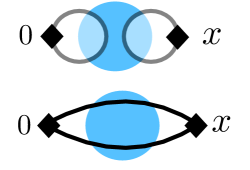
Figure 13: Two diagrams for in-vacuum correlation functions. The rhombuses correspond to two operators $\left<{\cal O}(0){\cal O}(x)\right>$ inserted at Euclidean coordinates $0$ and $x\sim 1/Q$. The blue circles refer to a nonperturbative background field.

The point-to-point correlation functions on the lattice provided wave functions at the origin in the form of constants like $f_{\pi},\chi_{\pi},f_{\rho}$, needed for form factors. The strong splitting between the light $\pi-\sigma$ with $m_{\pi}^{2}\approx 0$ and $m_{\sigma}^{2}\approx 0.2\,{\rm GeV}^{2}$ on the one hand, and $\eta^{\prime}-\delta$ with $m_{\eta^{\prime},\delta}^{2}\sim 1\,{\rm GeV}^{2}$ on the other, historically provided a motivation for the dominance of instanton-induced forces described by the effective ’t Hooft Lagrangian

$${\cal O}_{\rm tHooft}\sim(\bar{u}_{L}u_{R})(\bar{d}_{L}d_{R})+(L\leftrightarrow R)$$

There are direct lattice evidences (e.g. Faccioli and DeGrand (2003)) that this operator is indeed dominant in the vacuum. One can certainly do now much more systematic lattice studies of multiple correlation functions at small/intermediate distances, and quantify the strength of all relevant 4-fermion operators

$${\cal O}_{\Gamma}=(\bar{q}\Gamma q)(\bar{q}\Gamma q)$$

That will put the NJL-type modeling of quark-quark forces on a more quantitative basis.

Let us also mention here another area in which an interesting phenomenology of quark interaction, in the same range of momentum transfer, has been developed: the physics of Pomerons and diffractive processes. In Fig. 14 we schematically show two basic processes, the high energy elastic scattering and the double-diffractive production (sometimes called Pomeron-Pomeron collisions).

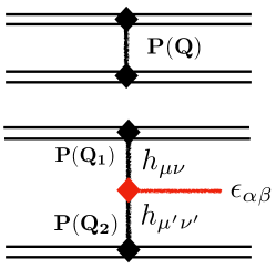
Figure 14: Elastic high energy collision of hadrons (upper) and double-diffractive production of a hadron (lower plot). Note that Pomeron-Pomeron-(tensor) Hadron may have many different index structures, but it is the “triple-graviton” one which explains the data Iatrakis et al. (2016).

In the lowest perturbative order, the Pomeron is just a $two-gluon$ exchange. In higher orders it is given by ladder diagrams producing the so called BFKL Pomeron Kuraev et al. (1977); Balitsky and Lipatov (1978). At intermediate $Q$ one also think of it as (Reggeized) exchange of glueballs. It is worth recalling, that the first one on the Pomeron trajectory is not the lowest scalar glueball, but a tensor one $J^{PC}=2^{++}$. This correlates well with recent demonstrations Iatrakis et al. (2016); Ewerz et al. (2016) that the Pomeron is also an object possessing a symmetric polarization $tensor$ $h^{\mu\nu}$. Finally, note that in the holographic models of QCD the Pomeron and tensor glueballs are just certain parts of Reggeized graviton exchanges that sum up to a close string exchange Rho et al. (1999); Brower et al. (2007). Taking this into account, one may expect to find among the quark-quark forces the operator containing the product of two stress tensors

$${\cal O}_{TT}=(\bar{q}\partial_{\mu}\gamma_{\nu}q)(\bar{q}\partial_{\mu}\gamma_{\nu}q)$$

The problem however remains: we do not entirely understand the mechanisms of the quark-antiquark scattering , at any level of precision. The instantons are not the only nonperturbative objects in the QCD vacuum. The (nearly 60 years old) NJL Lagrangian is very important, but still it is not the only quark interaction.

VI.2 Where should further progress happen?

As we emphasized in the Introduction, in spite of significant efforts, experimental measurements of the pion and kaon form factors have hardly entered the semi-hard domain of $Q^{2}$ discussed. Perhaps with a new facility such as the EIC in Brookhaven, there will be further experimental progress.

In the near future, we anticipate a rapid progress in lattice calculations of the mesonic form factors. The simulations with physical light masses are currently possible, and the subtleties of chiral dynamics are under control.

Current lattice studies (of the vector pion form factors in Brandt (2013); Alexandrou et al. (2018) and scalar form factors Gülpers et al. (2014)) are restricted to momentum transfer range $Q^{2}<1\,{\rm GeV}^{2}$. In order to get to larger momentum transfer, one needs lattices with smaller lattice spacing. With this in mind we have picked up a sample of mesonic form factors carried by the HPQCD collaboration, see Fig. 15. The strategy of HPQCD is to approach the problem gradually, from heavier to lighter quarks. The natural expectation is that the physics of the heavy quark system is simpler, since their nonrelativistic wave functions, and some other aspects are under better theoretical control. Heavier quark flavors are expected to be less involved in nonperturbative interactions. Starting with the $b,c$ system, and going down to the strange quarks, we note that they become more relativistic, and more sensitive to the details of chiral symmetry breaking and its nonperturbative origins. On the lattice one can of course dial any value for the quark masses.

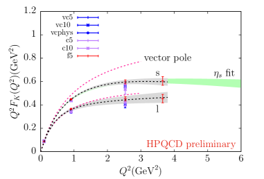
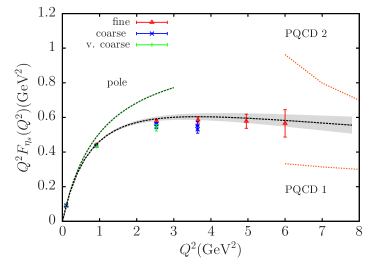
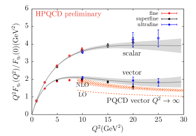
Figure 15: Mesonic form factors calculated on the lattice by the HPQCD collaboration: $K$-meson Davies et al. (2018), $\eta_{s}$ Koponen et al. (2017) and $\eta_{c}$ Davies et al. (2018), top to bottom.

In the vector channels, mesons made of different flavors do not mix much, and one might think that the $\rho\rightarrow\phi\rightarrow J/\psi$ sequence can be smoothly connected via a change in mass. However in the light pseudoscalar channels we know the mixing is very strong. Furthermore, it is complicated by the broken chiral U${}_{A}(1)$ symmetry, due to which $\eta^{\prime}$ is not a partner to the octet states at all. (This is a strong indication of the dominance of ’t Hooft-like interaction, which is flavor-nondiagonal by construction.)

In order not to deal with such issues, in Koponen et al. (2017), an artificial particle called $\eta_{s}$ was invented. It is different from the physical $\eta$ or $\eta^{\prime}$. Its definition can be explained as follows: imagine that there are two more species of strange quarks, $s^{\prime}$ and $s^{\prime\prime}$, which have the same mass as the standard $m_{s}$. Their additional properties are: (i) they are not identical, so the pair $\bar{s}^{\prime}s"$ cannot annihilate, and the correlators consist only of the connected one-loop diagram, while the (very costly) disconnected two-loop diagram does not exist. This construction avoids the calculation of that diagram which is technically challenging; (ii) Also for simplicity, one of these presumed quarks is given an electric charge $e_{s^{\prime}}=1$, and the other one neutral, with $e_{s^{\prime\prime}}=0$, eliminating half of the diagrams. It was numerically found that in the range $Q^{2}\approx 2-9\,{\rm GeV}^{2}$, the $\eta_{s}$ form factor times $Q^{2}$

$$Q^{2}F_{\eta_{s}}(Q^{2})\approx 0.6\,{\rm GeV}^{2}$$ (141)

is approximatly constant, with no indication to reach the pQCD asymptotic value, which is significantly smaller. Almost identical results were recently obtained for the $K$ meson form factor.

For the charmed $\eta_{c}$ meson, the vector form factor was calculated to significantly higher momentum transfer $Q^{2}\sim 25\,{\rm GeV}^{2}$. Again, $Q^{2}F_{\eta_{s}}$ remains approximately constant, also about twice larger than the asymptotic value. Lattice data for the scalar form factor indicate that it (times $Q^{2}$) is also about constant, in contradiction with the chirality flip suppression rule predicted by the gluon exchange mechanism. Furthermore, the numerical value of this constant is $larger$ than for vector form factor, by another factor 2!

Multi-gluon diagrams lead to a correction of order $(1+1.18\alpha_{s})$ Melic et al. (1999), that can partly help to bridge the gap between the lattice results and the pQCD for the vector form factor. However, this correction would not help for the scalar form factor, as gluon exchange cannot create the necessary chirality flip, except through a penalty factor $m_{f}/Q$. However, we explain the presence of scalar form factors by non-vanishing cross-terms, between two chiral structures in the distributions.

Taken literally, our calculations are done for zero current quark masses, while the lattice data under consideration are for massive $s,c$ quarks. So, they are not related directly. But, the strange quark mass is small enough $m_{s}^{2}\ll Q^{2}$, and it should not matter much, and in fact it can perhaps be included perturbatively in the propagators. What we found is that the sum of the perturbative contribution with $Q^{2}F(Q^{2})$ weakly growing with $Q^{2}$, plus the instanton contributions, amounts to a near-constant as observed on fine lattices by the HPQCD collaboration.

The lattice configurations can be made “more smooth” by various procedures (e.g., the gradient flow) by which one can gradually remove high-momentum gluons, while keeping instantons (the action minima). Measuring formfactors during such procedure, one is expected to see the results changing, to their respective versions including only instanton-induced effects. Our calculations can therefore be considered as predictions for formfactors, modified by such smoothening procedures.

Finally, instantons are only some fraction of the nonperturbative forces between quarks. We just calculated what we could. Instantons are the only background for which full massless quark propagators are available. It may well be that, with better measurements/calculations of these formfactors one may need some non-perturbative mechanisms of quark-antiquark interactions, other than the one-gluon exchange and instantons. Perhaps, for heavy quarks, one can proceed along the line of Ref Chernyshev et al. (1996), starting from the heavy quark limit.

Acknowledgements

One of us (ES) thanks Vladimir Braun and the other organizers of the Mainz 2019 workshop on light-front distribution amplitudes for the invitation, to its participants, and in particular Christine Davies, whose talk triggered the present work. We thank Viktor Chernyak for helpful comments on the first version of our paper. This work is supported by the Office of Science, U.S. Department of Energy under Contract No. DE-FG-88ER40388.

Appendix A Notations and kinematics

The definition of momenta are given in Fig.1(a). Note that in the Breit frame the initial meson momentum $p_{\mu}=(0,0,-Q/2,Q/2)$, and the final meson momentum is $p^{\prime}_{\mu}=(0,0,Q/2,Q/2)$, where we ignored the meson mass $p_{\mu}^{2}\approx 0$. Note that we put the energy as the 4-th component rather than the 0-th as we do in Euclidean notations, and that we call the two first components $transverse$, for the momenta and polarization vectors.

Since we consider as an example mesons with charge $+1$ or $\bar{d}u$ flavors, the upper line in Fig.1(a) corresponds to a $u$ quark, and its direction is assumed to be left-to-right. The other line ($\bar{d}$ with underlined momenta $\underline{k}_{i}$) has flow of baryon charge in the opposite direction, right-to-left, which is reflected in the definition of its momenta with opposite sign. Therefore, in our notations

$$p^{\mu}=k_{1}^{\mu}-\underline{k}_{1}^{\mu},\,\,\,\,{p^{\prime}}^{\mu}=k_{2}^{\mu}-\underline{k}_{2}^{\mu}$$

For completeness, let us mention that momentum conservation corresponds to $p^{\mu}+q^{\mu}={p^{\prime}}^{\mu}$. In Minkowskian kinematic we use the standard Dirac “slash” notations

$$p/\hskip 2.58334pt\equiv p^{\mu}\gamma_{\mu}$$

Our set of gamma matrices are in the chiral basis, meaning that $\gamma_{5}$ is diagonal.

Appendix B Instanton field and its Fourier transform

Throughout, we will use the conventions and notations developed in Balitsky et al. (1993); Moch et al. (1997); Vandoren and van Nieuwenhuizen (2008) for the instanton calculus. Superposition of instantons only makes sense if they are all in the so called singular gauge

$$A^{a}_{\mu}(x)={2\over g}\bar{\eta}^{a}_{\mu\nu}{\rho^{2}(x_{\nu}-z_{\nu})\over(x-z)^{2}((x-z)^{2}+\rho^{2})}$$ (142)

$$={2\over g}\bar{\eta}^{a}_{\mu\nu}(x_{\nu}-z_{\nu})\big{[}{1\over(x-z)^{2}}-{1\over((x-z)^{2}+\rho^{2})}\big{]}$$

All Fourier transforms will be carried using

$$\mathbb{F}(\pm k)\equiv\int d^{4}x\,e^{\mp ik\cdot x}\,\mathbb{F}(x)$$ (143)

The instanton Fourier transform is

$$A^{a}_{\mu}(k)={4\pi^{2}\over g}\bar{\eta}^{a}_{\mu\nu}{\partial\over\partial k_{\nu}}\bigg{(}{1\over k^{2}}-{\rho\over k}K_{1}(k\rho)\bigg{)}$$ (144)

where $K_{1}$ is the Bessel function. Quite characteristically, one finds two terms, one decaying as a power of $k$ as $\langle A^{*}_{\mu}(k)A_{\mu}(k)\rangle\sim n/k^{6}$, supplemented by a term which decreases exponentially at large k, $\sim e^{-k\rho}$. The former term comes from the point-like gauge topological singularity at the origin $\sim x_{\nu}/x^{2}$, and therefore it does not depend on instanton size $\rho$. It is spurious. The latter originates from the regular bracket.

Following Balitsky et al. (1993); Moch et al. (1997); Vandoren and van Nieuwenhuizen (2008), we use the short hand matrix-valued notation $x\equiv\sigma_{\mu}x^{\mu}$ and $\overline{x}\equiv\overline{\sigma}_{\mu}x^{\nu}$, with the covariantized Pauli matrices in Euclidean and Minkowski space defined as

$${\rm Euclidean}: \qquad\sigma_{\mu}=(1,-i\vec{\sigma})\qquad\overline{\sigma}_{\mu}=(1,+i\vec{\sigma})\qquad\sigma_{\mu}\overline{\sigma}_{\nu}+\sigma_{\nu}\overline{\sigma}_{\mu}=2\eta_{\mu\nu}$$

$${\rm Minkowski}: \qquad\sigma_{\mu}=(1,-\vec{\sigma})\qquad\overline{\sigma}_{\mu}=(1,+\vec{\sigma})\qquad\sigma_{\mu}\overline{\sigma}_{\nu}+\sigma_{\nu}\overline{\sigma}_{\mu}=2g_{\mu\nu}$$

with metric $g^{\mu\nu}=(+,-,-,-)$, $\eta^{\mu\nu}=\delta^{\mu\nu}$, and satisfying the identities

$$\sigma^{\mu}\overline{\sigma}^{\nu}-\sigma^{\nu}\overline{\sigma}^{\mu}=2i\overline{\eta}^{a\mu\nu}\tau^{a}\qquad\qquad\overline{\sigma}^{\mu}{\sigma}^{\nu}-\overline{\sigma}^{\nu}{\sigma}^{\mu}=2i{\eta}^{a\mu\nu}\tau^{a}$$ (145)

with the $\eta$-tHooft symbol. The spinor indices are $\alpha,\beta=1,2$, and the color indices are $i,j=1,2,...N_{c}$. We will carry the analytical continuation from Euclidean to Minkowski space using the prescription for space-like momenta $q_{M}^{2}\leq 0$

$$q_{E}^{2}\rightarrow-q_{M}^{2}+i0\qquad\qquad\rho\sqrt{q_{E}^{2}}\rightarrow\rho\sqrt{-q_{M}^{2}}\$$ (146)

For time-like momenta $q_{M}^{2}>0$, it is more appropriate to use the double prescription

$$q_{E}^{2}\rightarrow-q_{M}^{2}+i0\qquad\qquad\rho\sqrt{q_{E}^{2}}\rightarrow\rho\sqrt{q_{M}^{2}}\qquad\qquad{\rm arg}\rho=-{\rm arg}\sqrt{q^{2}}$$ (147)

The analytical continuation in the instanton size $\rho\rightarrow-i\rho$ compensates for the extra phase obtained when analytically continuing in momentum. Since we are formally integrating over the instanton size distribution which is fixed by the saddle point, this continuation is absorbed by the $\rho$-integration measure (116).

Appendix C Fermionic zero modes

Our conventions for the $\gamma^{5}$ matrix in Euclidean and Minkowski space are respectively

$$\gamma_{E}^{5}=\begin{pmatrix}-1&0\\ 0&1\end{pmatrix}\qquad\qquad\gamma_{M}^{5}=\begin{pmatrix}1&0\\ 0&-1\end{pmatrix}$$ (148)

In Weyl notations, the Euclidean Dirac spinor reads

$$\Psi(x) = \begin{pmatrix}K^{i}_{\alpha}(x)\\ \phi^{\alpha}_{i}(x)\\ \end{pmatrix}\qquad\Psi^{\dagger}(x)=({K}_{i}^{\dagger\alpha}(x),\phi_{\alpha}^{\dagger i}(x))\equiv(\overline{\phi}^{\alpha}_{i}(x),\overline{K}^{i}_{\alpha}(x))$$ (149)

The Euclidean fermionic action splits into left $K$ and right $\phi$ copies

$$\overline{K}\sigma\cdot(\partial-igA)K+\overline{\phi}\,\overline{\sigma}\cdot(\partial-igA)\phi$$ (150)

with $\overline{K}=\phi^{\dagger}$ and $\overline{\phi}=K^{\dagger}$ using

$$\gamma_{E}^{\mu}=\begin{pmatrix}0&\bar{\sigma}_{E}^{\mu}\\ \sigma_{E}^{\mu}&0\end{pmatrix}\qquad\qquad\gamma_{M}^{\mu}=\begin{pmatrix}0&\bar{\sigma}_{M}^{\mu}\\ \sigma_{M}^{\mu}&0\end{pmatrix}$$ (151)

The instanton admits a left-handed zero mode $K^{i}_{\alpha}(x)$ satisfying $\sigma\cdot D\,K=0$, and the anti-instanton a right-handed zero mode $\phi^{\alpha}_{i}(x)$ satisfying $\overline{\sigma}\cdot D\,\phi=0$, which are eigenstates of $(1\pm\gamma_{E}^{5})/2$, and conjugate of each other. In terms of the Euclidean Weyl spinors, the instanton zero mode and its conjugate are

$$K^{i}_{\alpha}(x) = \frac{\rho^{\frac{3}{2}}}{\pi x^{4}}\frac{(\overline{x}\epsilon U)^{i}_{\alpha}}{\Pi_{x}^{\frac{3}{2}}}=\frac{2\pi\rho^{\frac{3}{2}}}{\Pi_{x}^{\frac{3}{2}}}\,(\overline{S}_{0}(x)\epsilon U)^{i}_{\alpha}$$

$$K^{\dagger\alpha}_{i}(x) = \frac{\rho^{\frac{3}{2}}}{\pi x^{4}}\frac{(U^{\dagger}\epsilon x)^{\alpha}_{i}}{x^{4}\Pi_{x}^{\frac{3}{2}}}=\frac{2\pi\rho^{\frac{3}{2}}}{\Pi_{x}^{\frac{3}{2}}}\,(U^{\dagger}\epsilon{S}_{0}(x))_{i}^{\alpha}\equiv{\overline{\phi}}^{\alpha}_{i}(x)$$ (152)

Here $\epsilon$ is the antisymmetric spin 2-tensor with the normalization $\epsilon_{\alpha\sigma}\epsilon^{\sigma\beta}=\delta_{\alpha}^{\beta}$, and

$$\Pi_{x}=1+\frac{\rho^{2}}{x^{2}}\qquad S_{0}(x)=\frac{x}{2\pi^{2}x^{4}}\qquad\overline{S}_{0}(x)=\frac{\overline{x}}{2\pi^{2}x^{4}}$$ (153)

with $S_{0}(x)$ the free massless quark propagator. The zero modes are normalized to $\rho$,

$$\int d^{4}x\,K^{\dagger}(x)K(x)=\rho\qquad\qquad\int d^{4}x\,\phi^{\dagger}(x)\phi(x)=\rho$$ (154)

For the free Dirac spinors we will use the notation $\chi(k)=\chi_{R}(k)+\chi_{L}(k)$ (with Minkowski labeling) as the sum of free Weyl spinors, that satisfy

$$\not{k}\chi(k)=\not{k}\begin{pmatrix}\chi_{R}(k)\\ \chi_{L}(k)\\ \end{pmatrix}=\begin{pmatrix}0&\overline{k}\\ k&0\\ \end{pmatrix}\begin{pmatrix}\chi_{R}(k)\\ \chi_{L}(k)\\ \end{pmatrix}=\begin{pmatrix}\overline{k}\chi_{L}(k)\\ k\chi_{R}(k)\\ \end{pmatrix}=0$$ (155)

with the free-wave ortho-normalizations

$$\chi_{L,R}(k)\chi_{L,R}^{\dagger}(k)=k,\overline{k}\qquad\qquad\chi^{\dagger}_{L,R}(k)\chi_{R,L}(k)=0$$ (156)

Appendix D Details of the averaging in (IV.1)

The first bracket in (IV.1),

$$\left<k_{2}\left|{\partial}\,\overline{S}\,\overline{\epsilon}(q)\,\overline{S}\,{\partial}\,\frac{1+\gamma_{5}}{2}+\overline{\partial}\,{S}\,{\epsilon}(q)\,{S}\,\overline{\partial}\,\frac{1-\gamma_{5}}{2}\right|k_{1}\right>$$ (157)

when converted to the configuration representation, is dominated by the large $x,y$-asymptotics of the propagators on mass-shell. This translates formally to $\overline{S}(x,z)\rightarrow\overline{S}_{0}(x-z)/\sqrt{\Pi_{z}}$ to the left, and $\overline{S}(z,y)\rightarrow\overline{S}_{0}(z-y)/\sqrt{\Pi_{z}}$ to the right, and similarly for ${S}(x,z)$ and ${S}(z,y)$. With this in mind, (157) gives

$$\left(\overline{\epsilon}(q)\frac{1+\gamma_{5}}{2}+\epsilon(q)\frac{1-\gamma_{5}}{2}\right)\,\int d^{4}z\,\frac{e^{iq\cdot z}}{\Pi_{z}}$$ (158)

independently of the color orientations $U$ with

$$\int d^{4}z\,\frac{e^{iq\cdot z}}{\Pi_{z}}=-{\partial_{q}^{2}}\int d^{4}z\,{e^{iq\cdot z}}\int_{0}^{\infty}d\lambda\,e^{-\lambda(z^{2}+\rho^{2})}=-4\pi^{2}\rho^{4}\,\bigg{(}\frac{K_{1}(\xi)}{\xi}\bigg{)}^{\prime\prime}_{\xi=\rho q}$$ (159)

which at large $q$ asymptotes $\sim e^{-\rho q}/(\rho q)^{3/2}$, plus an additional contribution

$$\bigg{(}\frac{1}{ik_{2}}\sigma_{\mu}\,[U\sigma_{\mu}\,(-i\overline{\partial}_{q})\,U^{\dagger}]\,\epsilon(q)\left(\frac{1-\gamma_{5}}{2}\right)$$

$$-\,\overline{\epsilon}(q)\,\overline{\sigma}_{\mu}\,[U(-i\partial_{q})\,\overline{\sigma}_{\mu}\,U^{\dagger}]\,\frac{1}{i\overline{k}_{1}}\left(\frac{1+\gamma_{5}}{2}\right)\,\bigg{)}\,\int d^{4}z\,{e^{iq\cdot z}}\,\frac{\rho^{2}}{z^{4}\Pi_{z}^{2}}$$

which depends on the color orientations with

$$\int d^{4}z\,{e^{iq\cdot z}}\,\frac{\rho^{2}}{z^{4}\Pi^{2}_{z}}=-\rho^{2}{\partial\over\partial\rho^{2}}\int d^{4}z\,{e^{iq\cdot z}}\,\frac{1}{z^{2}+\rho^{2}}=-2\pi^{2}\rho^{2}\,\bigg{(}\frac{(\xi K_{1}(\xi))^{\prime}}{\xi}\bigg{)}_{\xi=q\rho}$$ (161)

which asymptotes $\sim e^{-\rho q}/(\rho q)^{1/2}$.

The contribution (159) amounts to the instanton contribution to the electric form factor on a single quark line. To understand the electric or magnetic nature of the contribution (D-161), we average it over the instanton color moduli using the identity

$$\int dU\,U^{i}_{\alpha}\,U^{\dagger\beta}_{j}=\frac{1}{N_{c}}\delta^{i}_{j}\delta^{\beta}_{\alpha}$$ (162)

to have

$$\bigg{(}-\frac{\overline{k}_{2}}{k^{2}_{2}}\,q\,\epsilon(q)\left(\frac{1-\gamma_{5}}{2}\right)+\,\overline{\epsilon}(q)\,\overline{q}\,\frac{k_{1}}{k^{2}_{1}}\left(\frac{1+\gamma_{5}}{2}\right)\,\bigg{)}\,\bigg{(}-\frac{4\pi^{2}\rho^{4}}{N_{c}}\,\frac{1}{\xi}\bigg{(}\frac{(\xi K_{1})^{\prime}}{\xi}\bigg{)}^{\prime}\bigg{)}$$ (163)

On a single quark line with $q=k_{2}-k_{1}$ and both ends on mass-shell, (163) yields the vector vertex

$$\frac{q^{2}}{M_{Q}^{2}}\bigg{(}1+{\cal O}\bigg{(}\frac{k_{1,2}}{q}\bigg{)}\bigg{)}\,\left(\overline{\epsilon}(q)\frac{1+\gamma_{5}}{2}+\epsilon(q)\frac{1-\gamma_{5}}{2}\right)\,\bigg{(}-\frac{4\pi^{2}\rho^{4}}{N_{c}}\,\frac{1}{\xi}\bigg{(}\frac{(\xi K_{1})^{\prime}}{\xi}\bigg{)}^{\prime}\bigg{)}$$ (164)

We regulated the emerging poles using $k_{1,2}^{2}=0\rightarrow-M_{Q}^{2}$ in Euclidean signature. (164) is seen as an additional instanton contribution to the electric form factor of a single quark line, much like (159).

The second bracket in (IV.1)

$$\left<\underline{k}_{1}\left|{\partial}\,\overline{S}\,{\partial}\,\frac{1+\gamma_{5}}{2}+\overline{\partial}\,{S}\,\overline{\partial}\,\frac{1-\gamma_{5}}{2}\right|\underline{k}_{2}\right>\$$ (165)

can be LSZ reduced exactly. More specifically, applying the LSZ reduction to the right of the second term in (165) and retaining only the leading $\underline{k}_{2}^{2}\rightarrow 0$ contribution give

$$\bigg{[}\int d^{4}x\,{e^{-i({\underline{k}_{2}-\underline{k}_{1})\cdot x}}}\,\frac{i\overline{\underline{k}}_{1}}{\sqrt{\Pi_{x}}}\bigg{(}1+\frac{\rho^{2}}{2x^{2}}\frac{[Ux\underline{\overline{k}}_{2}U^{\dagger}]}{\underline{k}_{2}\cdot x}\bigg{(}1-e^{i\underline{k}_{2}\cdot x}\bigg{)}\bigg{)}+{\cal O}(\underline{k}_{2})\bigg{]}\,\frac{1-\gamma_{5}}{2}$$ (166)

Similarly, applying the LSZ reduction to the left of the first term in (165) and retaining only the leading $\underline{k}_{1}^{2}\rightarrow 0$ contribution give

$$\bigg{[}\int d^{4}x\,{e^{-i({\underline{k}_{2}-\underline{k}_{1})\cdot x}}}\,\bigg{(}1+\frac{\rho^{2}}{2x^{2}}\frac{[U\underline{k}_{1}\overline{x}U^{\dagger}]}{\underline{k}_{1}\cdot x}\bigg{(}1-e^{-i\underline{k}_{1}\cdot x}\bigg{)}\bigg{)}\,\frac{i{\underline{k}}_{2}}{\sqrt{\Pi_{x}}}+{\cal O}(\underline{k}_{1})\bigg{]}\,\frac{1+\gamma_{5}}{2}$$ (167)

In the limit $\underline{k}_{1,2}\rightarrow 0$, the contributions in (166-167) do not vanish unless the integrals develop singularities which can only arise from the large x-asymptotic of the integrands, as the contributions for $x\approx 0$ are all finite. For instance, for a single quark line (167) after color averaging gives

$${i{\underline{k}}_{2}}\int d^{4}x\,{e^{-i(\underline{k}_{2}-\underline{k}_{1})\cdot x}}\,\bigg{(}1+\frac{\rho^{2}}{2N_{c}x^{2}}\bigg{(}1-e^{-i\underline{k}_{1}\cdot x}\bigg{)}\bigg{)}\frac{1}{\sqrt{\Pi_{x}}}+{\cal O}(\underline{k}_{1})$$

$$= {i{\underline{k}}_{2}}\,\bigg{(}(2\pi)^{4}\,\delta^{4}(\underline{k}_{2}-\underline{k}_{1})-\frac{2\pi^{2}\rho^{2}}{{(\underline{k}_{2}-\underline{k}_{1})}^{2}}\bigg{(}1-\frac{1}{N_{c}}\bigg{)}-\frac{2\pi^{2}\rho^{2}}{{\underline{k}}_{2}^{2}}\,\frac{1}{N_{c}}\bigg{)}+{\cal O}(\underline{k}_{1,2})$$

$$\approx {i{\underline{k}}_{2}}\,\bigg{(}(2\pi)^{4}\,\delta^{4}(\underline{k}_{2})-\frac{2\pi^{2}\rho^{2}}{{\underline{k}}_{2}^{2}}\bigg{(}\bigg{(}1-\frac{1}{N_{c}}\bigg{)}+\frac{1}{N_{c}}\bigg{)}\bigg{)}+{\cal O}(\underline{k}_{1,2})$$ (168)

with the approximation $\underline{k}_{2}-\underline{k}_{1}\approx\underline{k}_{2}$ near the Euclidean mass shell. This approximation supports retaining only the 1-contribution in (166-167), with the final result in Euclidean signature

$${2\pi^{2}\rho^{2}}\,\bigg{(}\bigg{(}1-\frac{1}{N_{c}}\bigg{)}+\frac{1}{N_{c}}\bigg{)}\,\bigg{(}\frac{1}{i{\underline{k}}_{1}}\frac{1-\gamma_{5}}{2}+\frac{1}{i\overline{\underline{k}}_{2}}\frac{1+\gamma_{5}}{2}\bigg{)}$$ (169)

Appendix E Rules for the diagrams with zero modes insertion

In Fig. 16 we illustrate the LSZ reduced Feynman diagram for incoming and outgoing waves stemming from an instanton zero mode. We note that the LSZ reduction is not guaranteed unless the Euclidean field theory has a Hamiltonian interpretation, which is lacking in the instanton model of the QCD vacuum. Here it is understood as an algorithm. More specifically, each LSZ reduced diagram corresponds to

$${\rm Fig}.~{}\ref{fig_fr1}A = \int d^{4}x_{1}\,\overline{\phi}(x_{1})\overleftarrow{\overline{\partial}}_{x_{1}}\chi_{L}(k_{1})e^{-ik_{1}\cdot x_{1}}=\overline{\phi}(k_{1})(i\overline{k})\chi_{L}(k_{1})$$

$${\rm Fig}.~{}\ref{fig_fr1}B = \int d^{4}x_{1}\,\chi_{R}^{\dagger}(k_{2})\overrightarrow{\partial}_{x_{1}}K(x_{1})e^{+ik_{2}\cdot x_{1}}=\chi_{R}^{\dagger}(k_{2})(-ik_{2})K(-k_{2})$$

$${\rm Fig}.~{}\ref{fig_fr1}C = \int d^{4}x_{1}\,\overline{\phi}(x_{1})\overleftarrow{\overline{\partial}}_{x_{1}}\chi_{L}(\underline{k}_{2})e^{+i\underline{k}_{2}\cdot x_{1}}=\overline{\phi}(-\underline{k}_{2})(-i\overline{\underline{k}}_{2})\chi_{L}(\underline{k}_{2})$$

$${\rm Fig}.~{}\ref{fig_fr1}D = \int d^{4}x_{1}\,\chi_{R}^{\dagger}(\underline{k}_{1})\overrightarrow{\partial}_{x_{1}}K(x_{1})e^{-i\underline{k}_{1}\cdot x_{1}}=\chi_{R}^{\dagger}(\underline{k}_{1})(i\underline{k}_{1})K(\underline{k}_{1})$$

with the instanton localized at $Z=0$. The integration over the collective $Z$-location of the instanton (anti-instanton) in a given diagram gives rise to overall 4-momentum conservation

$$(2\pi)^{4}\delta(k_{1}+\underline{k}_{1}+q-k_{2}-\underline{k}_{2})$$ (171)

The LSZ reduction of the quark zero modes (C) amounts to the amputation of the free quark propagator in the large-x limit with $\Pi_{x}\rightarrow 1$. In momentum space this amounts to

$$\lim_{k^{2}\rightarrow 0}\chi_{R}^{\dagger}(k)\,ik\,K^{i}(-k)=-2\pi\rho^{\frac{3}{2}}\chi_{R\alpha}^{\dagger}(k)\epsilon^{\alpha\beta}U^{i}_{\beta}$$

$$\lim_{k^{2}\rightarrow 0}\overline{\phi}_{j}(-k)(-i\overline{k})\chi_{L}(k)=+2\pi\rho^{\frac{3}{2}}U^{\dagger\beta}_{j}\epsilon_{\beta\alpha}\chi_{L}^{\alpha}(k)$$ (172)

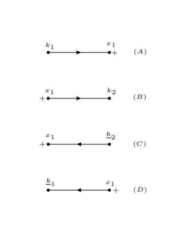
Figure 16: Quark (A,B) and antiquark (C,D) zero modes entering and exiting an instanton labeled by $+$.

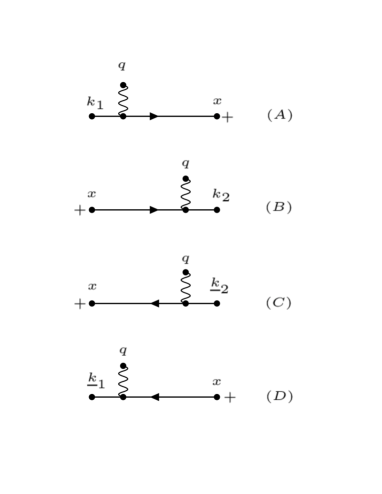
Figure 17: Quark (A,B) and antiquark (C,D) absorbing or emitting a vector photon in an instanton background labeled by $+$.

In Fig. 17 we show the Feyman graphs whereby a zero mode absorbs a virtual vector with polarization $\epsilon_{\mu}(q)$ (absorption) and flips to a non-zero mode. The same rules apply for a scalar or a pseudoscalar vertex with the polarization set to $\pm 1$. The extention to the energy-momentum tensor vertex were given above. Following the definitions established earlier, each of the vertex gives

$${\rm Fig}.~{}\ref{fig_fr2}A = \epsilon(q)\cdot{V}(q,k_{1})\equiv\int d^{4}x\,e^{-iq\cdot x}\overline{\phi}(x)\,\overline{\epsilon}(q)\,S(x,k_{1})$$

$${\rm Fig}.~{}\ref{fig_fr2}B = \epsilon(q)\cdot\overline{V}(q,-{k}_{2})\equiv\int d^{4}x\,e^{-iq\cdot x}\overline{S}(-k_{2},x)\,\epsilon(q)\,K(x)$$

$${\rm Fig}.~{}\ref{fig_fr2}C = \epsilon(q)\cdot{V}(q,-\underline{k}_{2})\equiv\int d^{4}x\,e^{-iq\cdot x}\overline{\phi}(x)\,\overline{\epsilon}(q)\,S(x,-\underline{k}_{2})$$

$${\rm Fig}.~{}\ref{fig_fr2}D = \epsilon(q)\cdot\overline{V}(q,\underline{k}_{1})\equiv\int d^{4}x\,e^{-iq\cdot x}\overline{S}(\underline{k}_{1},x)\,\epsilon(q)\,K(x)$$ (173)

The mixed Fourier transform of the non-zero mode propagators in Weyl form, follows from (143) using

$$S(x,y)=\bigg{(}S_{0}(x-y)\bigg{(}1+\rho^{2}\frac{Ux\bar{y}U^{\dagger}}{x^{2}y^{2}}\bigg{)}+\frac{\rho^{2}\sigma_{\mu}}{4\pi^{2}}\frac{Ux(\bar{x}-\bar{y})\sigma_{\mu}\bar{y}U^{\dagger}}{x^{2}(x-y)^{2}y^{4}\Pi_{y}}\bigg{)}\,\frac{1}{(\Pi_{x}\Pi_{y})^{\frac{1}{2}}}$$

$$\overline{S}(x,y)=\bigg{(}\overline{S}_{0}(x-y)\bigg{(}1+\rho^{2}\frac{Ux\bar{y}U^{\dagger}}{x^{2}y^{2}}\bigg{)}+\frac{\rho^{2}\overline{\sigma}_{\mu}}{4\pi^{2}}\frac{Ux\overline{\sigma}_{\mu}(x-y)\bar{y}U^{\dagger}}{\Pi_{x}x^{4}(x-y)^{2}y^{2}}\bigg{)}\,\frac{1}{(\Pi_{x}\Pi_{y})^{\frac{1}{2}}}$$ (174)

More specifically, the LSZ amputated propagators $S\bar{k}$ and $k\overline{S}$ are found to be

$$ik\overline{S}(k,y) \approx \frac{e^{+ik\cdot y}}{\Pi^{1/2}_{y}}\bigg{(}1+\frac{\rho^{2}}{2y^{2}}\frac{Uk\bar{y}U^{\dagger}}{k\cdot y}(1-e^{-ik\cdot y})\bigg{)}$$

$${S}(x,k)i\bar{k} \approx \frac{e^{-ik\cdot x}}{\Pi^{1/2}_{x}}\bigg{(}1+\frac{\rho^{2}}{2x^{2}}\frac{Ux\bar{k}U^{\dagger}}{k\cdot x}(1-e^{+ik\cdot x})\bigg{)}$$ (175)

in agreement with those originally found in Moch et al. (1997). The new and more involved LSZ amputations $\overline{S}k$ and $\bar{k}S$ are

$$\overline{S}(x,k)ik \approx \frac{e^{-ik\cdot x}}{\Pi^{1/2}_{x}}\bigg{(}1-\frac{\rho^{2}}{2x^{2}}\frac{Uk\bar{x}U^{\dagger}}{k\cdot x}\bigg{(}1-\frac{i}{k\cdot x}(1-e^{+ik\cdot x})\bigg{)}-\frac{\rho^{2}}{M_{Q}^{2}}\frac{ik}{x^{4}\Pi_{x}}\bar{\sigma}_{\mu}U{x}\bar{\sigma}_{\mu}U^{\dagger}\bigg{)}$$

$$i\bar{k}{S}(k,y) \approx \frac{e^{+ik\cdot y}}{\Pi^{1/2}_{y}}\bigg{(}1-\frac{\rho^{2}}{2y^{2}}\frac{Uy\bar{k}U^{\dagger}}{k\cdot y}\bigg{(}1+\frac{i}{k\cdot y}(1-e^{-ik\cdot y})\bigg{)}-\frac{\rho^{2}}{M_{Q}^{2}}\frac{i\bar{k}}{y^{4}\Pi_{+}}\sigma_{\mu}U\sigma_{\mu}\bar{y}U^{\dagger}\bigg{)}$$

Note that we made use of the Euclidean regulator $-k^{2}\approx 0\rightarrow M_{Q}^{2}$ in the last contributions appearing in (E). The LSZ amputated parts of the vertices in Figs. 17A,B read

$$\lim_{k_{1}^{2}\rightarrow 0}\epsilon(q)\cdot{V}(q,{k}_{1})(i\overline{k}_{1})=$$

$$+(i2\pi\rho^{\frac{3}{2}})U^{\dagger}\bigg{(}\frac{\epsilon{k}_{1}\overline{\epsilon}(q)}{2k_{1}\cdot q}F(\rho\sqrt{q^{2}})+\bigg{(}\frac{\epsilon(q+k_{1})\overline{\epsilon}(q)}{(q+k_{1})^{2}}-\frac{\epsilon k_{1}\overline{\epsilon}(q)}{2k_{1}\cdot q}\bigg{)}F(\rho\sqrt{(q+k_{1})^{2}})\bigg{)}$$

$$\lim_{k_{2}^{2}\rightarrow 0}(-ik_{2})\epsilon(q)\cdot\overline{V}(q,-{k}_{2})=$$

$$-(i2\pi\rho^{\frac{3}{2}})\bigg{(}\frac{\epsilon(q)\overline{k}_{2}{\epsilon}}{2k_{2}\cdot q}F(\rho\sqrt{q^{2}})+\bigg{(}\frac{\epsilon(q)(\overline{q}-\overline{k}_{2}){\epsilon}}{(q-k_{2})^{2}}-\frac{\epsilon(q)\overline{k}_{2}{\epsilon}}{2k_{2}\cdot q}\bigg{)}F(\rho\sqrt{(q-k_{2})^{2}})\bigg{)}U$$

respectively, and similarly for Figs. 17C,D with $F(x)=xK_{1}(x)$ in terms of the Mac-Donald function.

Appendix F Scalar vertex redux

If we ignore the transverse momentum dependence in the vertices, a simpler derivation of the vector, scalar and gravitational vertices in the instanton background can be obtained. Here, we illustrate it for the case of the scalar insertion. Typically, we have

$$\tilde{\cal S}(q,k_{1})=\int d^{4}xe^{-iq\cdot x}\overline{\phi}(x)S(x,k_{1})=\int d^{4}xe^{-iq\cdot x}\overline{\phi}(x)\,\overline{\sigma}_{\mu}{\overrightarrow{D}}_{\mu}\Delta(x,k_{1})$$ (178)

with $\Delta(x,k_{1})$ the half-mass shell Fourier transform of the scalar propagator in (64). Here since $\sigma_{\mu}D_{\mu}K(x)=0$ with $K^{\dagger}=\overline{\phi}$ (149), it is easier to proceed through the integration by parts and obtain

$$\tilde{\cal S}(q,k_{1})=\int d^{4}xe^{-iq\cdot x}\overline{\phi}(x)\,i\bar{q}\,\Delta(x,k_{1})\approx\int d^{4}xe^{-iq\cdot x}\overline{\phi}(x)\,\frac{i\bar{q}}{\sqrt{\Pi_{x}}}\,\Delta_{0}(x,k_{1})$$ (179)

with the free scalar propagator $\Delta_{0}(x,k_{1})=e^{ik_{1}\cdot x}/k_{1}^{2}$ and $k_{1}^{2}$ on mass shell. Inserting the instanton zero mode in (179) and carrying the integration give ($\xi=\rho\sqrt{q^{2}}$)

$$\tilde{\cal S}(q,k_{1})\approx\frac{2\pi\rho^{7/2}q^{2}\,K_{1}(\xi)}{k_{1}^{2}\xi}\,(U^{\dagger}\epsilon ik_{1})$$ (180)

In terms of (180) the scalar vertex reads

$$\bigg{[}\bigg{(}\frac{8\kappa q^{2}K_{1}(\xi)}{-k_{1}^{2}\xi}\bigg{)}(\chi^{\dagger}_{R}(k_{2})\epsilon U)\bigg{(}U^{\dagger}\epsilon\frac{k_{1}}{2M_{Q}}\chi_{R}(k_{1})\bigg{)}+(\chi^{\dagger}_{L}(k_{2})\epsilon U)\bigg{(}U^{\dagger}\epsilon\frac{\bar{k}_{2}}{2M_{Q}}\chi_{L}(k_{1})\bigg{)}\bigg{]}$$

$$\times\bigg{[}\frac{(2\pi\rho)^{2}}{M_{Q}}(\chi_{R}^{\dagger}(\underline{k}_{1})\epsilon U)(U^{\dagger}\epsilon\chi_{L}(\underline{k}_{2}))\bigg{]}$$ (181)

(F) is in agreement with (106) after analytical continuation with $k_{1}^{2}\approx 0\rightarrow-M_{Q}^{2}$ and color averaging.

Appendix G Fierzing vector and scalar

Further rearrangements at the expense of length can be done using Fierzing to recombine the color contractions., through the identity

$$(\overline{\psi}{\bf M}\phi)\,(\overline{\omega}{\bf N}\lambda)=-\frac{1}{4}\sum_{\cal O}\,(\overline{\psi}{\cal O}\lambda)\,(\overline{\omega}{\bf N}{\cal O}{\bf M}\phi)$$ (182)

with ${\cal O}={\bf 1},\gamma_{5},\gamma_{\mu},i\gamma_{5}\gamma_{\mu},i\gamma_{\mu}\gamma_{\nu}$. More specifically, the subleading contributions in $1/N_{c}$ in (IV.6) can be cast in the form

$$e_{u}\times\bigg{(}\frac{-1}{N_{c}(N_{c}^{2}-1)}\bigg{)}\bigg{(}\frac{-1}{4}\bigg{)}$$

$$\times\bigg{[}\,\,2\,\bigg{(}\overline{u}_{R}(k_{2})d_{L}(\underline{k}_{2})\bigg{)}\bigg{(}\overline{d}_{R}(\underline{k}_{1})(\mathbb{F}_{V}(q,k_{1})+\mathbb{F}_{V}(q,-k_{2}))u_{L}(k_{1})\bigg{)}$$

$$\,\,\,\,\,\,-\,\bigg{(}\overline{u}_{R}(k_{2})\gamma_{\mu}\gamma_{\nu}d_{L}(\underline{k}_{2})\bigg{)}\bigg{(}\overline{d}_{R}(\underline{k}_{1})\gamma^{\mu}\gamma^{\nu}(\mathbb{F}_{V}(q,k_{1})+\mathbb{F}_{V}(q,-k_{2}))u_{L}(k_{1})\bigg{)}$$

$$\,\,\,\,\,\,+2\,\bigg{(}\overline{u}_{R}(k_{2})u_{L}(k_{1})\bigg{)}\bigg{(}\overline{d}_{R}(\underline{k}_{1})(\mathbb{F}_{V}(q,k_{1})+\mathbb{F}_{V}(q,-k_{2}))d_{L}(\underline{k}_{2})\bigg{)}$$

$$\,\,\,\,\,\,-\,\bigg{(}\overline{u}_{R}(k_{2})\gamma_{\mu}\gamma_{\nu}u_{L}(k_{1})\bigg{)}\bigg{(}\overline{d}_{R}(\underline{k}_{1})\gamma^{\mu}\gamma^{\nu}(\mathbb{F}_{V}(q,k_{1})+\mathbb{F}_{V}(q,-k_{2}))d_{L}(\underline{k}_{2})\bigg{)}\bigg{]}$$ (183)

and

$$e_{\overline{d}}\times\bigg{(}\frac{-1}{N_{c}(N_{c}^{2}-1)}\bigg{)}\bigg{(}\frac{-1}{4}\bigg{)}$$

$$\times\bigg{[}\,\,2\bigg{(}\overline{u}_{R}(k_{2})d_{L}(\underline{k}_{2})\bigg{)}\bigg{(}\overline{d}_{R}(\underline{k}_{1})(\mathbb{F}_{V}(q,\underline{k}_{1})+\mathbb{F}_{V}(q,-\underline{k}_{2}))u_{L}(k_{1})\bigg{)}$$

$$-\bigg{(}\overline{u}_{R}(k_{2})\gamma_{\mu}\gamma_{\nu}d_{L}(\underline{k}_{2})\bigg{)}\bigg{(}\overline{d}_{R}(\underline{k}_{1})(\mathbb{F}_{V}(q,\underline{k}_{1})+\mathbb{F}_{V}(q,-\underline{k}_{2}))\gamma^{\mu}\gamma^{\nu}u_{L}(k_{1})$$

$$\,\,+2\bigg{(}\overline{u}_{R}(k_{2})u_{L}(k_{1})\bigg{)}\bigg{(}\overline{d}_{R}(\underline{k}_{1})\mathbb{(}\mathbb{F}_{V}(q,\underline{k}_{1})+\mathbb{F}_{V}(q,-\underline{k}_{2}))d_{L}(\underline{k}_{2})\bigg{)}$$

$$-\bigg{(}\overline{u}_{R}(k_{2})\gamma_{\mu}\gamma_{\nu}u_{L}(k_{1})\bigg{)}\bigg{(}\overline{d}_{R}(\underline{k}_{1})(\mathbb{F}_{V}(q,\underline{k}_{1})+\mathbb{F}_{V}(q,-\underline{k}_{2}))\gamma^{\mu}\gamma^{\nu}d_{L}(\underline{k}_{2})\bigg{)}\bigg{]}$$ (184)

The subleading contributions in $1/N_{c}$ in (IV.7) can be Fierzed using (182) with the result

$$e_{u}\times\bigg{(}-\frac{1}{N_{c}(N_{c}^{2}-1)}\bigg{)}\bigg{(}-\frac{1}{4}\bigg{)}$$

$$\bigg{[}\bigg{(}\overline{u}_{L}(k_{2})\gamma_{\mu}u_{L}(k_{1})\bigg{)}\bigg{(}\overline{d}_{R}(\underline{k}_{1})\gamma^{\mu}\mathbb{F}_{S}(q,-k_{2})d_{L}(\underline{k}_{2})\bigg{)}$$

$$-\bigg{(}\overline{u}_{L}(k_{2})\gamma_{\mu}\gamma^{5}u_{L}(k_{1})\bigg{)}\bigg{(}\overline{d}_{R}(\underline{k}_{1})\gamma^{\mu}\gamma^{5}\mathbb{F}_{S}(q,-k_{2})d_{L}(\underline{k}_{2})\bigg{)}$$

$$+2\bigg{(}\overline{d}_{R}(\underline{k}_{1})d_{L}(\underline{k}_{2})\bigg{)}\bigg{(}\overline{u}_{R}({k}_{2})\overline{\mathbb{F}}_{S}(q,k_{1})u_{R}({k}_{1})\bigg{)}$$

$$-\bigg{(}\overline{d}_{R}(\underline{k}_{1})\gamma_{\mu}\gamma_{\nu}d_{L}(\underline{k}_{2})\bigg{)}\bigg{(}\overline{u}_{R}({k}_{2})\gamma^{\mu}\gamma^{\nu}\overline{\mathbb{F}}_{S}(q,k_{1})u_{R}({k}_{1})\bigg{)}$$

$$+\bigg{(}\overline{u}_{L}(k_{2})\gamma_{\mu}d_{L}(\underline{k}_{2})\bigg{)}\bigg{(}\overline{d}_{R}(\underline{k}_{1})\gamma^{\mu}\overline{\mathbb{F}}_{S}(q,-k_{2})u_{L}(k_{1})\bigg{)}$$

$$-\bigg{(}\overline{u}_{L}(k_{2})\gamma_{\mu}\gamma^{5}d_{L}(\underline{k}_{2})\bigg{)}\bigg{(}\overline{d}_{R}(\underline{k}_{1})\gamma^{\mu}\gamma^{5}\overline{\mathbb{F}}_{S}(q,-k_{2})u_{L}(k_{1})\bigg{)}$$

$$+2\bigg{(}\overline{u}_{R}(k_{2})d^{i}_{L}(\underline{k}_{2})\bigg{)}\bigg{(}\overline{d}_{R}(\underline{k}_{1})\overline{\mathbb{F}}_{S}(q,k_{1})u_{R}(k_{1})\bigg{)}$$

$$-\bigg{(}\overline{u}_{R}(k_{2})\gamma_{\mu}\gamma_{\nu}d_{L}(\underline{k}_{2})\bigg{)}\bigg{(}\overline{d}_{R}(\underline{k}_{1})\gamma^{\mu}\gamma^{\nu}\overline{\mathbb{F}}_{S}(q,k_{1})u_{R}(k_{1})\bigg{)}\bigg{]}$$

and

$$e_{\overline{d}}\times\bigg{(}-\frac{1}{N_{c}(N_{c}^{2}-1)}\bigg{)}\bigg{(}-\frac{1}{4}\bigg{)}$$

$$\bigg{[}2\bigg{(}\overline{u}_{R}(k_{2})u_{L}(k_{1})\bigg{)}\bigg{(}\overline{d}_{R}(\underline{k}_{1})\mathbb{F}_{S}(q,-\underline{k}_{2})d_{R}(\underline{k}_{2})\bigg{)}$$

$$-\bigg{(}\overline{u}_{R}(k_{2})\gamma_{\mu}\gamma_{\nu}u_{L}(k_{1})\bigg{)}\bigg{(}\overline{d}_{R}(\underline{k}_{1})\gamma^{\mu}\gamma^{\nu}\mathbb{F}_{S}(q,-\underline{k}_{2})d_{R}(\underline{k}_{2})\bigg{)}$$

$$+\bigg{(}\overline{d}_{L}(\underline{k}_{1})\gamma_{\mu}d_{L}(\underline{k}_{2})\bigg{)}\bigg{(}\overline{u}_{R}(k_{2})\gamma^{\mu}\overline{\mathbb{F}}_{S}(q,\underline{k}_{1})u_{L}(k_{1})\bigg{)}$$

$$-\bigg{(}\overline{d}_{L}(\underline{k}_{1})\gamma_{\mu}\gamma^{5}d_{L}(\underline{k}_{2})\bigg{)}\bigg{(}\overline{u}_{R}(k_{2})\gamma^{\mu}\gamma^{5}\overline{\mathbb{F}}_{S}(q,\underline{k}_{1})u_{L}(k_{1})\bigg{)}$$

$$+\bigg{(}\overline{u}_{R}(k_{2})\gamma_{\mu}d_{R}(\underline{k}_{2})\bigg{)}\bigg{(}\overline{d}_{R}(\underline{k}_{1})\mathbb{F}_{S}(q,-\underline{k}_{2})\gamma^{\mu}u_{L}(k_{1})\bigg{)}$$

$$-\bigg{(}\overline{u}_{R}(k_{2})\gamma_{\mu}\gamma^{5}d_{R}(\underline{k}_{2})\bigg{)}\bigg{(}\overline{d}_{R}(\underline{k}_{1})\mathbb{F}_{S}(q,-\underline{k}_{2})\gamma^{\mu}\gamma^{5}u_{L}(k_{1})\bigg{)}$$

$$+2\bigg{(}\overline{u}_{R}(k_{2})d_{L}(\underline{k}_{2})\bigg{)}\bigg{(}\overline{d}_{L}(\underline{k}_{1})\overline{\mathbb{F}}_{S}(q,\underline{k}_{1})u_{L}(k_{1})\bigg{)}$$

$$-\bigg{(}\overline{u}_{R}(k_{2})\gamma_{\mu}\gamma_{\nu}d_{L}(\underline{k}_{2})\bigg{)}\bigg{(}\overline{d}_{L}(\underline{k}_{1})\overline{\mathbb{F}}_{S}(q,\underline{k}_{1})\gamma^{\mu}\gamma^{\nu}u_{L}(k_{1})\bigg{)}\bigg{]}$$ (186)

References

- Shuryak (1993) Edward V. Shuryak, “Correlation functions in the QCD vacuum,” Rev. Mod. Phys. 65, 1–46 (1993).
- Radyushkin (1994) A.V. Radyushkin, “Pion wave function from QCD sum rules with nonlocal condensates,” in Workshop on Continuous Advances in QCD (1994) pp. 238–248, arXiv:hep-ph/9406237 .
- Brodsky et al. (2011) Stanley J. Brodsky, Fu-Guang Cao, and Guy F. de Teramond, “Evolved QCD predictions for the meson-photon transition form factors,” Phys. Rev. D 84, 033001 (2011), arXiv:1104.3364 [hep-ph] .
- Chang et al. (2013) Lei Chang, I.C. Cloet, J.J. Cobos-Martinez, C.D. Roberts, S.M. Schmidt, and P.C. Tandy, “Imaging dynamical chiral symmetry breaking: pion wave function on the light front,” Phys. Rev. Lett. 110, 132001 (2013), arXiv:1301.0324 [nucl-th] .
- Jia and Vary (2019) Shaoyang Jia and James P. Vary, “Basis light front quantization for the charged light mesons with color singlet Nambu–Jona-Lasinio interactions,” Phys. Rev. C 99, 035206 (2019), arXiv:1811.08512 [nucl-th] .
- Shuryak (2019) Edward Shuryak, “Light-front wave functions of mesons, baryons, and pentaquarks with topology-induced local four-quark interaction,” Phys. Rev. D 100, 114018 (2019), arXiv:1908.10270 [hep-ph] .
- Broniowski and Ruiz Arriola (2017) Wojciech Broniowski and Enrique Ruiz Arriola, “Nonperturbative partonic quasidistributions of the pion from chiral quark models,” Phys. Lett. B 773, 385–390 (2017), arXiv:1707.09588 [hep-ph] .
- Petrov and Pobylitsa (1997) V.Yu. Petrov and P.V. Pobylitsa, “Pion wave function from the instanton vacuum model,” (1997), arXiv:hep-ph/9712203 .
- Anikin et al. (2001) I.V. Anikin, A.E. Dorokhov, and L. Tomio, “Pion distribution amplitude within the instanton model,” Phys. Atom. Nucl. 64, 1329–1336 (2001).
- Ji (2013) Xiangdong Ji, “Parton Physics on a Euclidean Lattice,” Phys. Rev. Lett. 110, 262002 (2013), arXiv:1305.1539 [hep-ph] .
- Ji et al. (2015) Xiangdong Ji, Andreas Schäfer, Xiaonu Xiong, and Jian-Hui Zhang, “One-Loop Matching for Generalized Parton Distributions,” Phys. Rev. D 92, 014039 (2015), arXiv:1506.00248 [hep-ph] .
- Zhang et al. (2017) Jian-Hui Zhang, Jiunn-Wei Chen, Xiangdong Ji, Luchang Jin, and Huey-Wen Lin, “Pion Distribution Amplitude from Lattice QCD,” Phys. Rev. D 95, 094514 (2017), arXiv:1702.00008 [hep-lat] .
- Kock et al. (2020) Arthur Kock, Yizhuang Liu, and Ismail Zahed, “Pion and kaon parton distributions in the QCD instanton vacuum,” Phys. Rev. D 102, 014039 (2020), arXiv:2004.01595 [hep-ph] .
- Brodsky and Farrar (1973) Stanley J. Brodsky and Glennys R. Farrar, “Scaling Laws at Large Transverse Momentum,” Phys. Rev. Lett. 31, 1153–1156 (1973).
- Chernyak and Zhitnitsky (1977) V.L. Chernyak and A.R. Zhitnitsky, “Asymptotic Behavior of Hadron Form-Factors in Quark Model. (In Russian),” JETP Lett. 25, 510 (1977).
- Radyushkin (1977) A.V. Radyushkin, “Deep Elastic Processes of Composite Particles in Field Theory and Asymptotic Freedom,” (1977), arXiv:hep-ph/0410276 .
- Braun et al. (2000) Vladimir M. Braun, A. Khodjamirian, and M. Maul, “Pion form-factor in QCD at intermediate momentum transfers,” Phys. Rev. D 61, 073004 (2000), arXiv:hep-ph/9907495 .
- Forkel and Nielsen (1995) Hilmar Forkel and Marina Nielsen, “The Electromagnetic pion form-factor and instantons,” Phys. Lett. B 345, 55–60 (1995), arXiv:hep-ph/9408396 .
- Blotz and Shuryak (1997) Andree Blotz and Edward V. Shuryak, “Pion electromagnetic form-factor in the instanton vacuum,” Phys. Rev. D 55, 4055–4065 (1997), arXiv:hep-ph/9606355 .
- Faccioli et al. (2003) P. Faccioli, A. Schwenk, and E.V. Shuryak, “Instanton contribution to the pion electromagnetic form-factor at Q**2 greater than 1-GeV**2,” Phys. Rev. D 67, 113009 (2003), arXiv:hep-ph/0202027 .
- Braguta and Onishchenko (2004) V.V. Braguta and A.I. Onishchenko, “Pion form-factor and QCD sum rules: Case of pseudoscalar current,” Phys. Lett. B 591, 255–266 (2004), arXiv:hep-ph/0311146 .
- Schäfer and Shuryak (2001) Thomas Schäfer and Edward V. Shuryak, “Implications of the ALEPH tau lepton decay data for perturbative and nonperturbative QCD,” Phys. Rev. Lett. 86, 3973–3976 (2001), arXiv:hep-ph/0010116 .
- Negele (1997) John W. Negele, “Insight into hadron structure from lattice QCD,” AIP Conf. Proc. 412, 3–17 (1997), arXiv:hep-lat/9709129 .
- Nambu and Jona-Lasinio (1961) Yoichiro Nambu and G. Jona-Lasinio, “Dynamical Model of Elementary Particles Based on an Analogy with Superconductivity. 1.” Phys. Rev. 122, 345–358 (1961).
- Bernard et al. (1987) Veronique Bernard, Ulf G. Meissner, and Ismail Zahed, “Properties of the Scalar Meson at Finite Density,” Phys. Rev. Lett. 59, 966 (1987).
- Klevansky (1992) S.P. Klevansky, “The Nambu-Jona-Lasinio model of quantum chromodynamics,” Rev. Mod. Phys. 64, 649–708 (1992).
- Hutauruk et al. (2018) Parada T.P. Hutauruk, Wolfgang Bentz, Ian C. Cloët, and Anthony W. Thomas, “Charge Symmetry Breaking Effects in Pion and Kaon Structure,” Phys. Rev. C 97, 055210 (2018), arXiv:1802.05511 [nucl-th] .
- Plant and Birse (1998) Robert S. Plant and Michael C. Birse, “Meson properties in an extended nonlocal NJL model,” Nucl. Phys. A 628, 607–644 (1998), arXiv:hep-ph/9705372 .
- Belavin et al. (1975) A.A. Belavin, Alexander M. Polyakov, A.S. Schwartz, and Yu.S. Tyupkin, “Pseudoparticle Solutions of the Yang-Mills Equations,” Phys. Lett. B 59, 85–87 (1975).
- ’t Hooft (1976) Gerard ’t Hooft, “Computation of the Quantum Effects Due to a Four-Dimensional Pseudoparticle,” Phys. Rev. D 14, 3432–3450 (1976), [Erratum: Phys.Rev.D 18, 2199 (1978)].
- Gross et al. (1981) David J. Gross, Robert D. Pisarski, and Laurence G. Yaffe, “QCD and Instantons at Finite Temperature,” Rev. Mod. Phys. 53, 43 (1981).
- Shuryak (1982a) Edward V. Shuryak, “The Role of Instantons in Quantum Chromodynamics. 1. Physical Vacuum,” Nucl. Phys. B 203, 93 (1982a).
- Schäfer and Shuryak (1998) Thomas Schäfer and Edward V. Shuryak, “Instantons in QCD,” Rev. Mod. Phys. 70, 323–426 (1998), arXiv:hep-ph/9610451 .
- Callan et al. (1978) Jr. Callan, Curtis G., Roger F. Dashen, David J. Gross, Frank Wilczek, and A. Zee, “The Effect of Instantons on the Heavy Quark Potential,” Phys. Rev. D 18, 4684 (1978).
- Shuryak and Zahed (2000) Edward V. Shuryak and Ismail Zahed, “Instanton induced effects in QCD high-energy scattering,” Phys. Rev. D 62, 085014 (2000), arXiv:hep-ph/0005152 .
- Athenodorou et al. (2018) A. Athenodorou, Ph. Boucaud, F. De Soto, J. Rodríguez-Quintero, and S. Zafeiropoulos, “Instanton liquid properties from lattice QCD,” JHEP 02, 140 (2018), arXiv:1801.10155 [hep-lat] .
- Boucaud et al. (2003) Philippe Boucaud, F. De Soto, A. Le Yaouanc, J.P. Leroy, J. Micheli, H. Moutarde, O. Pene, and J. Rodriguez-Quintero, “The Strong coupling constant at small momentum as an instanton detector,” JHEP 04, 005 (2003), arXiv:hep-ph/0212192 .
- Geshkenbein and Terentev (1982) B.V. Geshkenbein and M.V. Terentev, “THE ENHANCED POWER CORRECTION TO THE ASYMPTOTICS OF THE PION FORM-FACTOR,” Phys. Lett. B 117, 243–246 (1982).
- Chibisov and Zhitnitsky (1995) Boris Chibisov and Ariel R. Zhitnitsky, “Transverse momentum distribution in hadrons. What can we learn from QCD?” Phys. Rev. D 52, 5273–5283 (1995), arXiv:hep-ph/9503476 .
- Shuryak and Velkovsky (1994) Edward V. Shuryak and M. Velkovsky, “The Instanton density at finite temperatures,” Phys. Rev. D 50, 3323–3327 (1994), arXiv:hep-ph/9403381 .
- Brown et al. (1978) Lowell S. Brown, Robert D. Carlitz, Dennis B. Creamer, and Choon-kyu Lee, “Propagation Functions in Pseudoparticle Fields,” Phys. Rev. D 17, 1583 (1978).
- Shuryak (1982b) Edward V. Shuryak, “The Role of Instantons in Quantum Chromodynamics. 3. Quark - Gluon Plasma,” Nucl. Phys. B 203, 140–156 (1982b).
- Pisarski and Yaffe (1980) R.D. Pisarski and L.G. Yaffe, “THE DENSITY OF INSTANTONS AT FINITE TEMPERATURE,” Phys. Lett. B 97, 110–112 (1980).
- Shifman et al. (1980) Mikhail A. Shifman, A.I. Vainshtein, and Valentin I. Zakharov, “Instanton Density in a Theory with Massless Quarks,” Nucl. Phys. B 163, 46–56 (1980).
- Faccioli and Shuryak (2001) P. Faccioli and Edward V. Shuryak, “Systematic study of the single instanton approximation in QCD,” Phys. Rev. D 64, 114020 (2001), arXiv:hep-ph/0106019 .
- Faccioli and DeGrand (2003) Pietro Faccioli and Thomas A. DeGrand, “Evidence for instanton induced dynamics, from lattice QCD,” Phys. Rev. Lett. 91, 182001 (2003), arXiv:hep-ph/0304219 .
- Kochelev (2003) N.I. Kochelev, “The Pauli form-factor of the quark induced by instantons,” Phys. Lett. B 565, 131–136 (2003), arXiv:hep-ph/0304171 .
- Hasenfratz (2000) Anna Hasenfratz, “Spatial correlation of the topological charge in pure SU(3) gauge theory and in QCD,” Phys. Lett. B 476, 188–192 (2000), arXiv:hep-lat/9912053 .
- Shuryak (1999) Edward V. Shuryak, “Probing the boundary of the nonperturbative QCD by small size instantons,” (1999), arXiv:hep-ph/9909458 .
- Lepage and Brodsky (1979) G.Peter Lepage and Stanley J. Brodsky, “Exclusive Processes in Quantum Chromodynamics: Evolution Equations for Hadronic Wave Functions and the Form-Factors of Mesons,” Phys. Lett. B 87, 359–365 (1979).
- Efremov and Radyushkin (1980) A.V. Efremov and A.V. Radyushkin, “Factorization and Asymptotical Behavior of Pion Form-Factor in QCD,” Phys. Lett. B 94, 245–250 (1980).
- Shuryak and Vainshtein (1982a) Edward V. Shuryak and A.I. Vainshtein, “Theory of Power Corrections to Deep Inelastic Scattering in Quantum Chromodynamics. 1. Q**2 Effects,” Nucl. Phys. B 199, 451–481 (1982a).
- Shuryak and Vainshtein (1982b) Edward V. Shuryak and A.I. Vainshtein, “Theory of Power Corrections to Deep Inelastic Scattering in Quantum Chromodynamics. 2. Q**4 Effects: Polarized Target,” Nucl. Phys. B 201, 141 (1982b).
- Ruiz Arriola and Broniowski (2002) Enrique Ruiz Arriola and Wojciech Broniowski, “Pion light cone wave function and pion distribution amplitude in the Nambu-Jona-Lasinio model,” Phys. Rev. D 66, 094016 (2002), arXiv:hep-ph/0207266 .
- Chernyak and Zhitnitsky (1984) V.L. Chernyak and A.R. Zhitnitsky, “Asymptotic Behavior of Exclusive Processes in QCD,” Phys. Rept. 112, 173 (1984).
- Petrov et al. (1999) V.Yu. Petrov, Maxim V. Polyakov, R. Ruskov, C. Weiss, and K. Goeke, “Pion and photon light cone wave functions from the instanton vacuum,” Phys. Rev. D 59, 114018 (1999), arXiv:hep-ph/9807229 .
- Polyakov and Weiss (1997) Maxim V. Polyakov and C. Weiss, “Nucleon structure functions from the instanton vacuum: Leading and nonleading twists,” Acta Phys. Polon. B 28, 2751–2764 (1997), arXiv:hep-ph/9709436 .
- Rapp et al. (1998) R. Rapp, Thomas Schäfer, Edward V. Shuryak, and M. Velkovsky, “Diquark Bose condensates in high density matter and instantons,” Phys. Rev. Lett. 81, 53–56 (1998), arXiv:hep-ph/9711396 .
- Ball and Braun (1996) Patricia Ball and Vladimir M. Braun, “The Rho meson light cone distribution amplitudes of leading twist revisited,” Phys. Rev. D 54, 2182–2193 (1996), arXiv:hep-ph/9602323 .
- Ball and Braun (1998) Patricia Ball and Vladimir M. Braun, “Handbook of higher twist distribution amplitudes of vector mesons in QCD,” in 3rd Workshop on Continuous Advances in QCD (QCD 98) (1998) pp. 125–141, arXiv:hep-ph/9808229 .
- Braun et al. (2017) Vladimir M. Braun et al., “The -meson light-cone distribution amplitudes from lattice QCD,” JHEP 04, 082 (2017), arXiv:1612.02955 [hep-lat] .
- Novikov et al. (1981) V.A. Novikov, Mikhail A. Shifman, A.I. Vainshtein, and Valentin I. Zakharov, “Are All Hadrons Alike? DESY-check = Moscow Inst. Theor. Exp. Phys. Gkae - Itef-81-048 (81,rec.jun.) 32 and Nucl. Phys. B191 (1981) 301-369 and Moscow Inst. Theor. Exp. Phys. Gkae - Itef-81-042 (81,rec.apr.) 70 . (104907),” Nucl. Phys. B 191, 301–369 (1981).
- Iatrakis et al. (2016) Ioannis Iatrakis, Adith Ramamurti, and Edward Shuryak, “Pomeron Interactions from the Einstein-Hilbert Action,” Phys. Rev. D 94, 045005 (2016), arXiv:1602.05014 [hep-ph] .
- Kuraev et al. (1977) E.A. Kuraev, L.N. Lipatov, and Victor S. Fadin, “The Pomeranchuk Singularity in Nonabelian Gauge Theories,” Sov. Phys. JETP 45, 199–204 (1977).
- Balitsky and Lipatov (1978) I.I. Balitsky and L.N. Lipatov, “The Pomeranchuk Singularity in Quantum Chromodynamics,” Sov. J. Nucl. Phys. 28, 822–829 (1978).
- Ewerz et al. (2016) Carlo Ewerz, Piotr Lebiedowicz, Otto Nachtmann, and Antoni Szczurek, “Helicity in proton–proton elastic scattering and the spin structure of the pomeron,” Phys. Lett. B 763, 382–387 (2016), arXiv:1606.08067 [hep-ph] .
- Rho et al. (1999) Mannque Rho, Sang-Jin Sin, and Ismail Zahed, “Elastic parton-parton scattering from AdS / CFT,” Phys. Lett. B 466, 199–205 (1999), arXiv:hep-th/9907126 .
- Brower et al. (2007) Richard C. Brower, Joseph Polchinski, Matthew J. Strassler, and Chung-I Tan, “The Pomeron and gauge/string duality,” JHEP 12, 005 (2007), arXiv:hep-th/0603115 .
- Brandt (2013) Bastian B. Brandt, “The electromagnetic form factor of the pion: Results from the lattice,” Int. J. Mod. Phys. E 22, 1330030 (2013), arXiv:1310.6389 [hep-lat] .
- Alexandrou et al. (2018) C. Alexandrou et al. (ETM), “Pion vector form factor from lattice QCD at the physical point,” Phys. Rev. D 97, 014508 (2018), arXiv:1710.10401 [hep-lat] .
- Gülpers et al. (2014) Vera Gülpers, Georg von Hippel, and Hartmut Wittig, “Scalar pion form factor in two-flavor lattice QCD,” Phys. Rev. D 89, 094503 (2014), arXiv:1309.2104 [hep-lat] .
- Davies et al. (2018) C.T.H. Davies, Jonna Koponen, Peter G. Lepage, Andrew T. Lytle, and Andre C. Zimermmane-Santos (HPQCD), “Meson Electromagnetic Form Factors from Lattice QCD,” PoS LATTICE2018, 298 (2018), arXiv:1902.03808 [hep-lat] .
- Koponen et al. (2017) J. Koponen, A.C. Zimermmane-Santos, C.T.H. Davies, G.P. Lepage, and A.T. Lytle, “Pseudoscalar meson electromagnetic form factor at high from full lattice QCD,” Phys. Rev. D 96, 054501 (2017), arXiv:1701.04250 [hep-lat] .
- Melic et al. (1999) B. Melic, B. Nizic, and K. Passek, “Complete next-to-leading order perturbative QCD prediction for the pion form-factor,” Phys. Rev. D 60, 074004 (1999), arXiv:hep-ph/9802204 .
- Chernyshev et al. (1996) S. Chernyshev, Maciej A. Nowak, and I. Zahed, “Heavy hadrons and QCD instantons,” Phys. Rev. D 53, 5176–5184 (1996), arXiv:hep-ph/9510326 .
- Balitsky et al. (1993) I.I. Balitsky, M. Beneke, and Vladimir M. Braun, “Instanton contributions to the tau decay widths,” Phys. Lett. B 318, 371–381 (1993), arXiv:hep-ph/9309217 .
- Moch et al. (1997) S. Moch, A. Ringwald, and F. Schrempp, “Instantons in deep inelastic scattering: The Simplest process,” Nucl. Phys. B 507, 134–156 (1997), arXiv:hep-ph/9609445 .
- Vandoren and van Nieuwenhuizen (2008) Stefan Vandoren and Peter van Nieuwenhuizen, “Lectures on instantons,” (2008), arXiv:0802.1862 [hep-th] .