Sequential Monte Carlo for Sampling Balanced and Compact Redistricting Plans

Abstract

Random sampling of graph partitions under constraints has become a popular tool for evaluating legislative redistricting plans. Analysts detect partisan gerrymandering by comparing a proposed redistricting plan with an ensemble of sampled alternative plans. For successful application, sampling methods must scale to maps with a moderate or large number of districts, incorporate realistic legal constraints, and accurately and efficiently sample from a selected target distribution. Unfortunately, most existing methods struggle in at least one of these areas. We present a new Sequential Monte Carlo (SMC) algorithm that generates a sample of redistricting plans converging to a realistic target distribution. Because it draws many plans in parallel, the SMC algorithm can efficiently explore the relevant space of redistricting plans better than the existing Markov chain Monte Carlo (MCMC) algorithms that generate plans sequentially. Our algorithm can simultaneously incorporate several constraints commonly imposed in real-world redistricting problems, including equal population, compactness, and preservation of administrative boundaries. We validate the accuracy of the proposed algorithm by using a small map where all redistricting plans can be enumerated. We then apply the SMC algorithm to evaluate the partisan implications of several maps submitted by relevant parties in a recent high-profile redistricting case in the state of Pennsylvania. We find that the proposed algorithm converges faster and with fewer samples than a comparable MCMC algorithm. Open-source software is available for implementing the proposed methodology.

Key Words: gerrymandering, graph partition, importance sampling, spanning trees

1 Introduction

In first-past-the-post electoral systems, legislative districts serve as the fundamental building block of democratic representation. In the United States, congressional redistricting, which redraws district boundaries in each state following the decennial Census, plays a central role in influencing who is elected and hence what policies are eventually enacted. Because the stakes are so high, redistricting has been subject to intense political battles. Parties often engage in gerrymandering by manipulating district boundaries in order to amplify the voting power of some groups while diluting that of others.

In recent years, the availability of granular data about individual voters has led to sophisticated partisan gerrymandering attempts that cannot be easily detected. At the same time, many scholars have focused their efforts on developing methods to uncover gerrymandering by comparing a proposed redistricting plan with a large collection of alternative plans that satisfy the relevant legal requirements. A primary advantage of such an approach over the use of simple summary statistics is its ability to account for the characteristics of each state’s physical and political geography and state-specific redistricting rules.

For its successful application, a sampling algorithm for drawing alternative plans must (1) be efficient enough to scale to maps with thousands of geographic units and a moderate or large number of districts, (2) simultaneously incorporate a variety of real-world legal constraints such as population balance (Section 3.1), geographical compactness (Section 3.3), and the preservation of administrative boundaries (Section 4.5), and (3) ensure these samples are representative of a specific target population, against which a redistricting plan of interest can be evaluated. Although some have been used in several recent court challenges to existing redistricting plans, all existing algorithms run into limitations of varying severity with regards to at least one of these three key requirements.

Optimization-based (e.g., Mehrotra et al.,, 1998; Macmillan,, 2001; Bozkaya et al.,, 2003; Liu et al.,, 2016) and constructive Monte Carlo (e.g., Cirincione et al.,, 2000; Chen and Rodden,, 2013; Magleby and Mosesson,, 2018) methods can be made scalable and incorporate many constraints. But they are not designed to sample from any specific target distribution. As a consequence, the resulting plans tend to differ systematically, for example, from a uniform distribution under certain constraints (Cho and Liu,, 2018; Fifield et al., 2020a, ; Fifield et al., 2020b, ). The absence of an explicit target distribution makes it difficult to interpret the ensembles generated by these methods and use them for statistical outlier analysis to detect gerrymandering.

MCMC algorithms (e.g., Mattingly and Vaughn,, 2014; Wu et al.,, 2015; Chikina et al.,, 2017; DeFord et al.,, 2021; Carter et al.,, 2019; Fifield et al., 2020a, ; Cannon et al.,, 2022) can in theory sample from a specific target distribution, and incorporate constraints through the use of an energy function. In practice, however, existing algorithms struggle to mix and traverse through a highly complex sampling space, making scalability difficult and accuracy hard to prove. Some of these algorithms make proposals by flipping precincts at the boundary of existing districts (e.g., Mattingly and Vaughn,, 2014; Fifield et al., 2020a, ), rendering it difficult or even impossible to transition between points in the state space, especially as more constraints are imposed. More recent algorithms by DeFord et al., (2021) and Carter et al., (2019) use spanning trees to make their proposals, and this has allowed these algorithms to yield greater moves and substantially improve mixing. Yet recent theoretical results suggest that even these larger moves may not be enough to traverse the entire state space, and therefore may fail to converge to the correct distribution, if a realistic population balance constraint is imposed (Akitaya et al.,, 2022).

We contribute to the ongoing scholarly efforts to address the above three key challenges by developing a new Sequential Monte Carlo (SMC) algorithm, based on a similar but not identical spanning tree construction to DeFord et al., (2021) and Carter et al., (2019) (see Sections 3 and 4). Like MCMC algorithms, the SMC algorithm generates samples which approximate the target distribution arbitrarily well as the sample size increases. But like constructive Monte Carlo methods, the SMC algorithm draws many separate plans from scratch, rather than tweaking a single plan sequentially. This approach is better suited to the large discrete state space with a multimodal target distribution that characterizes redistricting problems. For example, in cases where existing MCMC proposals render the state space disconnected, the SMC algorithm can still converge to the target distribution. As we demonstrate in Sections 5 and 6 (see also Appendix B), this sampling approach translates to faster convergence and smaller standard errors for a given computational budget. For larger and more complex redistricting sampling problems, the SMC algorithm can be easily parallelized to facilitate efficient computation.

The proposed algorithm proceeds by splitting off one district at a time, building up the redistricting plan piece by piece (see Figure 2 for an illustration). Each split is accomplished by drawing a spanning tree and removing one edge, which splits the spanning tree in two. We also extend the SMC algorithm so that it preserves administrative boundaries and certain geographical areas as much as possible, which is another common constraint considered in many real-world redistricting cases. An open-source software package, redist, is available for implementing the proposed algorithm (Kenny et al.,, 2020).

The SMC algorithm is not without limitations. Like existing MCMC approaches, the SMC algorithm only guarantees convergence to the target distribution as the sample size approaches infinity. Additionally, because the SMC algorithm involves repeated resampling, with a finite number of samples it can suffer from particle system collapse (Liu et al.,, 2001), significantly increasing sampling variability. Thus, it is important to understand the limitations of the proposed algorithm in finite samples, especially when dealing with large maps and many districts. In Section 4.4.4, we provide a set of diagnostics which can be used in practice to help identify if more samples are needed to reach convergence or if the constraints imposed by an analyst are too strong.

In Section 5, we validate the SMC algorithm using a small map for which all potential redistricting plans can be enumerated (Fifield et al., 2020b, ). We demonstrate that the proposed algorithm samples accurately from a realistic target distribution, and that our proposed diagnostics are a good proxy for total sampling error, which is generally unobservable. Section 6 applies the SMC algorithm to the 2011 Pennsylvania congressional redistricting, and also compares its performance on this problem with an MCMC algorithm with the same transition kernel as the proposed SMC algorithm. We find that the SMC algorithm samples more efficiently than the MCMC approach. Section 7 concludes and discusses directions for future work.

2 The 2011 Pennsylvania Congressional Redistricting

We study the 2011 Pennsylvania congressional redistricting because it illustrates the salient features of the redistricting problem. We begin by briefly summarizing the background of this case and then explain the role of sampling algorithms used in the expert witness reports.

2.1 Background

Pennsylvania lost a seat in Congress during the reapportionment of the 435 U.S. House seats following the 2010 Census. In Pennsylvania, the General Assembly, which is the state’s legislative body, draws new congressional districts, subject to gubernatorial veto. At the time, the General Assembly was controlled by Republicans, and Tom Corbett, also a Republican, served as governor. In the 2012 election, which took place under the newly adopted 2011 districting map, Democrats won 5 seats while Republicans took the remaining 13. Under the previous plan, the split was 7–12.

In June 2017, the League of Women Voters of Pennsylvania filed a lawsuit alleging that the 2011 plan adopted by the Republican legislature violated the state constitution by diluting the political power of Democratic voters. The case worked its way through the state court system, and on January 22, 2018, the Pennsylvania Supreme Court issued its ruling, writing that the 2011 plan “clearly, plainly and palpably violates the Constitution of the Commonwealth of Pennsylvania, and, on that sole basis, we hereby strike it as unconstitutional.” (League of Women Voters v. Commonwealth,, 2018).

The court ordered that the General Assembly adopt a remedial plan and submit it to the governor, who would in turn submit it to the court, by February 15, 2018. In its ruling, the court laid out specific requirements that had to be satisfied by all proposed plans:

composed of compact and contiguous territory; as nearly equal in population as practicable; and which do not divide any county, city, incorporated town, borough, township, or ward, except where necessary to ensure equality of population.

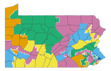
(a) 2011 General Assembly map

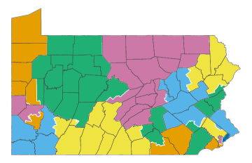
(b) 2018 Pennsylvania Supreme Court map

Figure 1: Comparison of the 2011 map drawn by the General Assembly and the final map imposed by the Supreme court in 2018. County lines are shown in dark gray, and district boundaries that do not coincide with county boundaries are in white.

The leaders of the Republican Party in the General Assembly drew a new map, but the Democratic governor, Tom Wolf, refused to submit it to the court, claiming that it, too, was an unconstitutional gerrymander. Instead, the court received remedial plans from seven parties: the petitioners, the League of Women Voters; the respondents, the Republican leaders of the General Assembly; the governor, a Democrat; the lieutenant governor, also a Democrat; the Democratic Pennsylvania House minority leadership; the Democratic Pennsylvania Senate minority leadership; and the intervenors, which included Republican party candidates and officials. Ultimately, the Supreme Court drew its own plan and adopted it on February 19, 2018, arguing that it was “superior or comparable to all plans submitted by the parties.” Figure 1 shows the remedial plan created by the Supreme Court as well as the 2011 map adopted by the General Assembly, which were found on the court’s case page.

The constraints explicitly laid out by the court, as well as the numerous remedial plans submitted by the parties, make the 2011 Pennsylvania redistricting a useful case study that evaluates redistricting plans.

2.2 The Role of Sampling Algorithms

The original finding that the 2011 General Assembly plan was a partisan gerrymander was in part based on different outlier analyses performed by two academic researchers, Jowei Chen and Wesley Pegden, who served as the petitioner’s expert witnesses. Chen randomly generated two sets of 500 redistricting plans according to a constructive Monte Carlo algorithm based on Chen and Rodden, (2013). He considered population balance, contiguity, compactness, avoiding county and municipal splits, and, in the second set of 500, avoiding plans that placed more than two incumbents in the same district (at least one pair of incumbents in the same district was necessary, given that Pennsylvania lost a seat from 2000 to 2010). Pegden ran a reversible Markov chain similar to that used in the MCMC algorithm of Mattingly and Vaughn, (2014) for one trillion steps, and computed upper bounds of $p$-values using the method of Chikina et al., (2017). This method was also used in a follow-up analysis by Moon Duchin, who served as an expert for Governor Wolf (Duchin,, 2018). Both petitioner experts concluded that the 2011 plan was an extreme outlier according to compactness, county and municipal splits, and the number of Republican and Democratic seats implied by statewide election results.

The respondents also retained an expert academic witness, Wendy Tam Cho, who directly addressed the sampling-based analyses of Chen and Pegden. Cho criticized Chen’s analysis for not sampling from a specified target distribution. She also criticized Pedgen’s analysis by arguing that his Markov chain only made local explorations of the space of redistricting plans, and could not therefore have generated a representative sample of all valid plans, though the $p$-values computed using the Chikina et al., (2017) method explicitly do not require mixing of the Markov chain (see also Cho and Rubinstein-Salzedo,, 2019, and Chikina et al., (2019)). We do not directly examine the intellectual merits of the specific arguments put forth by the expert witnesses. However, these methodological debates are also relevant for other cases where simulation algorithms have been extensively used by expert witnesses (e.g., Rucho v. Common Cause (2019); Common Cause v. Lewis (2019); Covington v. North Carolina (2017); Harper v. Lewis (2020)), and highlight the difficulties in practically applying existing sampling algorithms to actual redistricting problems.

First, the distributions that some of these algorithms sample from are not made explicit, leaving open the possibility that the generated ensemble is systematically different from the true set of all valid plans. Second, even when the distribution is known, MCMC algorithms used to sample from it may be prohibitively slow to mix and cannot yield a representative sample. These challenges motivate us to design an algorithm that accurately samples from a specific target distribution and incorporates most common redistricting constraints, while being efficient and scalable.

3 Sampling Balanced and Compact Districts

3.1 The Setup

Redistricting plans are ultimately aggregations of geographic units such as counties, voting precincts, or Census blocks. The usual requirement that the districts in a plan be contiguous necessitates consideration of the spatial relationship between these units. The natural mathematical structure for this consideration is a graph $G=(V,E)$, where $V=\{v_{1},v_{2},\ldots,v_{m}\}$ consists of $m$ nodes representing the geographic units of redistricting and $E$ contains edges connecting units which are legally adjacent.

A labeled redistricting plan on $G$ consists of $n$ districts, where each district is a collection of nodes. A labeled plan is described by a function $\xi:V\to\{1,2,\dots,n\}$, where $\xi(v)=i$ implies that node $v$ is in district $i$. In practice, we will be interested in unlabeled plans, since the assignment of sets of precincts to labels is arbitrary and has no impact on the real-world aspects of the district such as its population, demographic composition, or partisan lean. Define an equivalence relation by $\xi_{1}\cong\xi_{2}$ if there exists a permutation $\sigma$ such that $\xi_{1}(v)=\sigma(\xi_{2}(v))$ for all $v$. Then, an unlabeled redistricting plan can be viewed as an equivalence class under $\cong$, denoted $[\xi]$; nothing in what follows will depend on the particular labeled plan representative $\xi$.

We let $V_{i}(\xi)$ and $E_{i}(\xi)$ denote the nodes and edges contained in district $i$ under a given redistricting plan $\xi$, so $G_{i}(\xi)=(V_{i}(\xi),E_{i}(\xi))$ represents the induced subgraph that corresponds to district $i$ under the plan. We suppress the dependence on $\xi$ when it is clear from context, writing $G_{i}=(V_{i},E_{i})$. Since each node belongs to only one district, we have $V=\bigcup_{i=1}^{n}V_{i}(\xi)$ and $V_{i}(\xi)\bigcap V_{i^{\prime}}(\xi)=\varnothing$ for any redistricting plan $\xi$. In addition, we require that each district be contiguous, i.e., that $G_{i}$ is a connected graph, for all $i$.

Beyond connectedness, redistricting plans are always required to have roughly equal population in every district. To formalize this requirement, let $\operatorname{pop}(v)$ denote the population of node $v$. Then, the population of a district $i$ may be written as $\operatorname{pop}(V_{i}(\xi))\ \coloneqq\ \sum_{v\in V_{i}(\xi)}\operatorname{pop}(v)$. We quantify the discrepancy between a given plan and the ideal of equal population in every district by the maximum population deviation,

$$\operatorname{dev}(\xi)\ \coloneqq\ \max_{1\leq i\leq n}\absolutevalue{\frac{\operatorname{pop}(V_{i})}{\operatorname{pop}(V)/n}-1},$$

where $\operatorname{pop}(V)$ is the total population. Some courts and states have imposed hard maximums on this quantity, e.g., $\operatorname{dev}(\xi)\leq D=0.05$ for state legislative redistricting (National Conference of State Legislatures,, 2021).

The proposed algorithm samples plans by way of spanning trees on each district, i.e., subgraphs of $G_{i}(\xi)$ which contain all vertices, no cycles, and are connected. Let $T_{i}$ represent a spanning tree for district $i$ whose vertices and edges are given by $V_{i}(\xi)$ and a subset of $E_{i}(\xi)$, respectively. The collection of spanning trees from all districts together form a spanning forest. Each node belongs to one spanning tree in the forest, and this assignment corresponds to a redistricting plan. However, a single redistricting plan may correspond to multiple spanning forests because each district may admit more than one spanning tree.

For a given redistricting plan, we can compute the exact number of spanning forests in polynomial time using the determinant of a submatrix of the graph Laplacian, according to the Matrix Tree Theorem of Kirchhoff (see Tutte, (1984)). Thus, for a graph $H$, if we let $\tau(H)$ denote the number of spanning trees on the graph, we can represent the number of spanning forests that correspond to a redistricting plan $\xi$ as $\tau(\xi)\coloneqq\prod_{i=1}^{n}\tau(G_{i}(\xi))$. This fact will play an important role in the definition of our sampling algorithm and its target distribution.

3.2 The Target Distribution

The algorithm is designed to sample an unlabeled plan $[\xi]$ with probability

$$\pi([\xi])\propto\exp\{-J(\xi)\}\tau(\xi)^{\rho}\mathbf{1}_{\{\xi\text{ connected}\}}\mathbf{1}_{\{\operatorname{dev}(\xi)\leq D\}},$$ (1)

where the indicator functions ensure that the plans meet population balance and connectedness criteria, $\tau(\xi)$ measures the compactness of the districts in $\xi$ (see Section 3.3), and $J$ encodes additional constraints on the types of plans preferred. As done in Section 6, we often use a reasonably strict population constraint such as $D=0.001$ and $D=0.005$. The parameter $\rho\in\mathbb{R}_{0}^{+}$ is chosen to control the compactness of the generated plans.

This target distribution $\pi$ has both substantive and theoretical justifications. First, it incorporates two constraints which are almost always present in real-world redistricting: the support of $\pi$ is restricted to contiguous plans and those that meet a population deviation threshold. Second, it represents the unique maximum entropy distribution on the set of redistricting plans satisfying these two universal constraints and the moment conditions implied by the other constraints, i.e., $\operatorname{\mathbb{E}}_{\pi}[\log\tau(\xi)]=\mu_{\tau}$ and $\operatorname{\mathbb{E}}_{\pi}[J(\xi)]=\mu_{J}$ for some constants $\mu_{\tau}$ and $\mu_{J}$ (see Cover and Thomas,, 2006, Theorem. 12.1.1, originally of Boltzmann).

Thus, our target distribution ensures that all plans meet contiguity and population requirements, and on average satisfy a compactness standard as well as any other additional constraints (through the function $J$). It is no surprise, therefore, that this class of target distributions has been used by other work developing redistricting sampling algorithms (Herschlag et al.,, 2017; Fifield et al., 2020a, ).

The generality of the additional constraint function $J$ is intentional, as its exact form and number imposed on the redistricting process varies by state and by the type of districts being drawn; any type of constraint may be incorporated by choosing a $J$ which is small for preferred plans and large otherwise. For example, a preference for plans close to an existing plan $\xi_{\text{sq}}$ may be encoded as

$$J_{\text{sq}}(\xi) =-\frac{\beta}{\log n}\mathrm{VI}(\xi,\xi_{\text{sq}})\coloneqq-\frac{\beta}{2\log n}\sum_{i,j=1}^{n}\tfrac{P_{ij}}{\operatorname{pop}(V)}\quantity(\log(\tfrac{P_{ij}}{\operatorname{pop}(V_{j}(\xi_{\text{sq}}))})+\log(\tfrac{P_{ij}}{\operatorname{pop}(V_{j}(\xi))})),$$ (2)

where $\beta\in\mathbb{R}^{+}$ controls the strength of the constraint and $P_{ij}=\operatorname{pop}(V_{i}(\xi)\cap V_{j}(\xi_{\text{sq}}))$ is the population shared between district $i$ of $\xi$ and $j$ of $\xi_{\text{sq}}$. The function ${\rm VI}(\cdot,\cdot)$ represents the variation of information (also known as the shared information distance), which is the difference between the joint entropy and the mutual information of the distribution of population over the new districts $\xi$ relative to the existing districts $\xi_{sq}$ (Cover and Thomas,, 2006). When $\xi$ is any relabeling of $\xi_{\text{sq}}$, then $J_{\text{sq}}(\xi)=0$. In contrast, when $\xi$ evenly splits the nodes of each district of $\xi_{\text{sq}}$ among the districts of $\xi$, then $J_{\text{sq}}(\xi)=\beta$. This distance measure will prove useful later in quantifying the diversity of a sample of redistricting plans (see also Guth et al.,, 2020).

There exist other formulations of constraints, and considerations in choosing a set of weights that balance constraints against each other (see e.g., Bangia et al.,, 2017; Herschlag et al.,, 2017; Fifield et al., 2020a, ). Here, we focus on sampling from the broad class of distributions characterized by Equation (1), which have been used in other work; we do not address the important but separate problem of picking a specific instance of this class for a given redistricting problem.

The flexibility of $J$ can be deceptive, however. The algorithm operates efficiently only when the additional constraints imposed by $J$ are not too severe. Even a small number of strong constraints incorporated into $J$ can dramatically limit the number of valid plans and considerably complicate the process of sampling (Chatterjee and Diaconis,, 2018). The Markov chain algorithms developed to date partially avoid this problem by moving toward maps with lower $J$ over a number of steps, but in general including more constraints makes it even more difficult to transition between valid redistricting plans. Approaches such as simulated annealing (Bangia et al.,, 2017; Herschlag et al.,, 2017) and parallel tempering (Fifield et al., 2020a, ) have been proposed to handle multiple constraints, but these can be difficult to calibrate in practice and provide few, if any, theoretical guarantees.

In practice, we usually find that the most stringent constraints are those involving population deviation, compactness, and administrative boundary splits. As shown later, we address this issue by designing our algorithm to directly satisfy these constraints. Weak additional constraints do not generally have a substantial effect on the sampling efficiency, though there are exceptions. Monitoring the distribution of the weights and the overall sampling efficiency is crucial to obtaining a good sample, as we discuss later.

3.3 Spanning Forests and Compactness

One common redistricting requirement is that districts be geographically compact, though nearly every state leaves this term undefined. Dozens of numerical compactness measures have been proposed, with the Polsby–Popper score (Polsby and Popper,, 1991) perhaps the most popular. Defined as the ratio of a district’s area to that of a circle with the same perimeter as the district, the Polsby–Popper score is constrained to $[0,1]$, with higher scores indicating more compactness.

Other scholars have proposed a graph-theoretic measure known as edge-cut compactness (Dube and Clark,, 2016; DeFord et al.,, 2021). This measure counts the number of edges that must be removed from the original graph to partition it according to a given plan. Formally, it is defined as

$$\operatorname{rem}(\xi)\ \coloneqq\ 1-\frac{\sum_{i=1}^{n}|E_{i}(\xi)|}{|E(G)|},$$

where we have normalized to the total number of edges.

Plans that involve cutting many edges will necessarily have long internal boundaries, driving up their average district perimeter (and driving down their Polsby–Popper scores), while plans that cut as few edges as possible will have relatively short internal boundaries and much more compact districts. Additionally, given the high density of voting units in urban areas, plans which cut fewer edges will tend to avoid drawing district lines through the heart of these urban areas. This has the welcome side effect of avoiding splitting cities and towns, and in doing so helping to preserve “communities of interest,” another common redistricting consideration.

Empirically, this graph-based compactness measure is highly correlated with $\log\tau(G)-\log\tau(\xi)$ (we often observe a correlation in excess of 0.99). It is difficult to precisely characterize this relationship except in special cases because $\tau(\xi)$ is calculated as a matrix determinant (McKay,, 1981). However, this quantity is strongly controlled by the product of the degrees of each node in the graph, $\prod_{i=1}^{m}\deg(v_{i})$ (Kostochka,, 1995). Removing an edge from a graph decreases the degree of the vertices at either end by one, so we would expect $\log\tau(G)$ to change by approximately $2\{\log\bar{d}-\log(\bar{d}-1)\}$ with this edge removal, where $\bar{d}$ is the average degree of the graph. This implies a linear relation $\log\tau(G)-\log\tau(\xi)\approx\operatorname{rem}(\xi)\cdot 2\{\log\bar{d}-\log(\bar{d}-1)\}$, and hence $\tau(\xi)^{\rho}\approx C_{1}\exp(-C_{2}\,\rho\operatorname{rem}(\xi))$, where $C_{1}$ and $C_{2}$ are some constants depending on the details of the map.

As a result, a greater value of $\rho$ in the target distribution corresponds to a preference for fewer edge cuts and therefore a redistricting plan with more compact districts. This and the considerations given in the literature (Dube and Clark,, 2016; DeFord et al.,, 2021) suggest that the target distribution in Equation (1) with $\rho=1$ (or another positive value) is a good choice for sampling compact districts. The choice of $\rho=1$ is computationally convenient, as it allows us to avoid calculating $\tau(\xi)$ as part of sampling (an asymptotic bottleneck), and yet usually produces satisfactorily compact districts. Of course, if another compactness metric is desired, one can simply set $\rho=0$ and incorporate the alternative metric into $J$. This will preserve the algorithm’s efficiency to the extent that the alternative metric correlates with the edge-removal measure of compactness. Setting $\rho=0$ by itself, however, will make sampling intractable in most cases, just as choosing an extreme $J$ will.

4 The Proposed Algorithm

The proposed algorithm samples redistricting plans by sequentially drawing districts over $n-1$ iterations of a splitting procedure. This is fundamentally different from existing MCMC approaches, which change an existing plan according to some transition kernel. The iterations of the proposed algorithm are from district to district within a single plan whereas the iterations in an MCMC algorithm are from plan to plan.

Our algorithm begins by partitioning the original graph $G=(V,E)=(\widetilde{V}_{0},\widetilde{E}_{0})=\widetilde{G}_{0}$ into two induced subgraphs: $G_{1}=(V_{1},E_{1})$, which will constitute a district in the final map, and the remainder of the graph $\widetilde{G}_{1}=(\widetilde{V}_{1},\widetilde{E}_{1})$, where $\widetilde{V}_{1}=V\setminus V_{1}$ and $\widetilde{E}_{1}$ consists of all the edges between vertices in $\widetilde{V}_{1}$. Next, the algorithm takes $\widetilde{G}_{1}$ as an input graph and partitions it into two induced subgraphs, one which will become a district $G_{2}$ and the remaining graph $\widetilde{G}_{2}$. The algorithm repeats the same splitting procedure until the final $(n-1)$-th iteration whose two resulting partitions, $G_{n-1}$ and $\widetilde{G}_{n-1}=G_{n}$, become the final two districts of the redistricting plan.

(a) Initial map

(b) Iteration 1

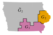
(c) Iteration 2

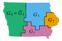
(d) Iteration 3

Figure 2: The sequential splitting procedure applied to the state of Iowa, where four congressional districts are created at the county level.

Figure 2 provides an illustration of this sequential procedure. To sample a large number of redistricting plans from the target distribution given in Equation (1), at each iteration, the algorithm samples many candidate partitions, discards those which fail to meet the population constraint, and then resamples a certain number of the remainder according to importance weights, using the resampled partitions at the next iteration. The rest of this section explains the details of the proposed algorithm.

4.1 The Splitting Procedure

We first describe the splitting procedure, which is similar to the merge-split Markov chain proposals of DeFord et al., (2021) and Carter et al., (2019). It proceeds by drawing a random spanning tree $T$, identifying the $k_{i}$ most promising edges to cut within the tree, and selecting one such edge at random to create two induced subgraphs. Spanning trees are an attractive way to split districts, as the removal of a single edge induces a partition with two connected components, and spanning trees can be sampled uniformly (Wilson,, 1996).

Algorithm 1 Splitting procedure to generate one district

Input: initial graph $\widetilde{G}_{i-1}$ and a parameter $k_{i}\in\mathbb{Z}^{+}$.

1. Draw a single spanning tree $T$ on $\widetilde{G}_{i-1}$ uniformly from the set of all such trees using Wilson’s algorithm.

2. Each edge $e\in E(T)$ divides $T$ into two components, $T_{e}^{(1)}$ and $T_{e}^{(2)}$. For each edge, compute the following population deviation for the two districts that would be induced by cutting $T$ at $e$,

   $$d_{e}^{(1)}\ =\ \absolutevalue{\frac{\sum_{v\in T_{e}^{(1)}}\operatorname{pop}(v)}{\operatorname{pop}(V)/n}-1}\mbox{\quad and\quad}d_{e}^{(2)}\ =\ \absolutevalue{\frac{\sum_{v\in T_{e}^{(2)}}\operatorname{pop}(v)}{\operatorname{pop}(V)/n}-1}.$$

   Let $d_{e}=\min\{d_{e}^{(1)},d_{e}^{(2)}\}$, and index the edges in ascending order by this quantity, so that we have $d_{e_{1}}\leq d_{e_{2}}\leq\cdots\leq d_{e_{m_{i}-1}}$, where $m_{i}=|\tilde{V}_{i-1}|$.

3. Select one edge $e^{*}$ uniformly from the top $k_{i}$ edges, $\{e_{1},e_{2},\dots,e_{k_{i}}\}$, and remove it from $T$, creating a spanning forest $(T_{e^{*}}^{(1)},T_{e^{*}}^{(2)})$ which induces a partition $(G_{i}^{(1)},G_{i}^{(2)})$.

4. If $d_{e^{*}}^{(1)}\leq d_{e^{*}}^{(2)}$, i.e., if $T_{e^{*}}^{(1)}$ induces a district that is closer to the optimal population than $T_{e^{*}}^{(2)}$ does, set $G_{i}=G_{i}^{(1)}$ and $\widetilde{G}_{i}=G_{i}^{(2)}$; otherwise, set $G_{i}=G_{i}^{(2)}$ and $\widetilde{G}_{i}=G_{i}^{(1)}$.

As part of the full sampling procedure (Algorithm 2), after splitting, we check that the population of the new district $G_{i}$ falls within the bounds $[P_{i}^{-},P_{i}^{+}]$ where

$$P_{i}^{-} =\max\quantity{\frac{\operatorname{pop}(V)}{n}(1-D),\ \operatorname{pop}(\widetilde{V}_{i-1})-\frac{n-i}{n}\operatorname{pop}(V)(1+D)}\mbox{\quad and\quad}$$

$$P_{i}^{+} =\min\quantity{\frac{\operatorname{pop}(V)}{n}(1+D),\ \operatorname{pop}(\widetilde{V}_{i-1})-\frac{n-i}{n}\operatorname{pop}(V)(1-D)}.$$

These bounds also ensure that it will be possible for future iterations to generate valid districts out of $\widetilde{G}_{i}$. If $\operatorname{pop}(V_{i})\not\in[P_{i}^{-},P_{i}^{+}]$, then the entire redistricting plan is rejected and the sampling process begins again. While the rate of rejection varies by map and by iteration, we generally encounter acceptance rates at each iteration between 5% and 30%, which are not so low as to make sampling from large maps intractable. Algorithm 1 details the steps of the splitting procedure, where at the first iteration we take $\widetilde{G}_{0}=G$.

4.2 The Sampling Probability

The above sequential splitting procedure does not generate plans from the target distribution $\pi$. We denote the sampling measure by $q$, and write the sampling probability for a given connected plan $\xi$ at iteration $i$ as $q(G_{i}\mid\widetilde{G}_{i-1})$, since each new district $G_{i}$ depends only on the leftover map area $\widetilde{G}_{i-1}$ from the previous iteration. This probability can be written as the probability that we cut an edge along the boundary of the new district, integrated over all spanning trees which could be cut to form the district, i.e.,

$$q(G_{i}\mid\widetilde{G}_{i-1})=\sum_{T\in\mathcal{T}(\widetilde{G}_{i-1})}q(G_{i}\mid T)\,\tau(\widetilde{G}_{i-1})^{-1},$$ (3)

where $\mathcal{T}(\cdot)$ represents the set of all spanning trees of a given graph, and we have relied on the fact that Wilson’s algorithm draws spanning trees uniformly.

The key is that for certain choices of $k_{i}$ (the number of edges considered to be cut at iteration $i$), the probability that an edge is cut is independent of the trees that are drawn. Let $ok(T)$ represent the number of edges on any spanning tree $T$ that induce balanced partitions with population deviation below $D$, i.e.,

$$ok(T)\ \coloneqq\ |\{e\in E(T):d_{e}\leq D\}|.$$

Then define $K_{i}\coloneqq\max_{T\in\mathcal{T}(\widetilde{G}_{i-1})}ok(T)$, the maximum number of such edges across all spanning trees. Furthermore, let $\mathcal{C}(G,H)$ represent the set of edges joining nodes in a subgraph $G$ to nodes in a subgraph $H$. We have the following result for the splitting probability for new districts whose populations lie inside the bounds defined above (Appendix A for the proof). lemmasplitprob The probability of splitting a valid new district $G_{i}$ from an existing area $\widetilde{G}_{i-1}$ using Algorithm 1 with parameter $k_{i}\geq K_{i}$ is

$$q(G_{i}\mid\widetilde{G}_{i-1},\operatorname{pop}(V_{i})\in[P_{i}^{-},P_{i}^{+}]) \ =\ \frac{\tau(G_{i})\tau(\widetilde{G}_{i})}{\tau(\widetilde{G}_{i-1})k_{i}}|\mathcal{C}(G_{i},\widetilde{G}_{i})|.$$ (4)

4.3 Sequential Monte Carlo

We follow a sequential Monte Carlo approach (Doucet et al.,, 2001; Liu et al.,, 2001) to generate draws from the target distribution, rather than simply performing $n-1$ iterations of Algorithm 1 and resampling or reweighting at the final stage. A sequential approach is also useful in operationalizing the rejection procedure to enforce the population constraint.

The proposed procedure is presented as Algorithm 2. The algorithm is governed by a parameter $\alpha\in(0,1]$, which has no effect on the target distribution nor the asymptotic accuracy of the algorithm. Rather, $\alpha$ may be adjusted to maximize the efficiency of sampling. To generate $S$ redistricting plans, at each iteration of the splitting procedure $i\in\{1,2,\dots,n-1\}$, we resample and split the existing plans one at a time, rejecting those which do not meet the population constraints, until we obtain $S$ new plans for the next iteration. This rejection process can be viewed as a form of partial rejection control (Liu et al.,, 1998, 2001), or a version of the AliveSMC algorithm (LeGland and Oudjane,, 2005; Peters et al.,, 2012).

The weights at each stage serve three purposes. The first is to account for the extraneous $|\mathcal{C}(G_{i},\widetilde{G}_{i})|$ term which appears in the splitting probability $q(G_{i}\mid\widetilde{G}_{i-1},\operatorname{pop}(V_{i})\in[P_{i}^{-},P_{i}^{+}])$ but not in the target distribution $\pi$. The second is to account for differences in the compactness parameter $\rho$; the splitting procedure generates plans according to $\rho=1$, but this may be different from the target value. The third purpose is to adjust for the imbalances between the labeled plans generated by the splitting procedure and the unlabeled plans which are the target of sampling. While there are $n!$ labeled plans corresponding to every unlabeled plan, not every labeled plan may be sampled according to the sequential procedure. In fact, the number of labeled plans which are in the support of the SMC proposal distribution varies from one unlabeled plan to another. It is this imbalance which necessitates an additional correction.

For a labeled plan $\xi$, let $G/\xi$ denote the district-level quotient graph corresponding to the plan; i.e., the nodes are districts $\{1,\dots,n\}$ and edges connect adjacent districts. Notice that the splitting procedure ensures that the leftover area after each split, $\widetilde{G}_{i}$, is a connected graph. This means that for every $1\leq i\leq n-1$, the subgraph of $G/\xi$ induced by the vertices $\{i+1,i+2,\dots,n\}$ (the districts drawn after split $i$) is connected. We call any labeled plan $\xi$ a sequentially valid labeling if this property holds, and denote by $\psi([\xi])$ the number of sequentially valid labelings corresponding to an unlabeled plan $[\xi]$. The SMC weights incorporate $\psi([\xi])$ as a correction term. Calculation of $\psi([\xi])$ is discussed below in Section 4.4.2.

Algorithm 2 Sequential Monte Carlo (SMC) Algorithm

Input: graph $G$ to be split into $n$ districts, target distribution parameters $\rho\in\mathbb{R}^{+}_{0}$ and constraint function $J$, and sampling parameters $\alpha\in(0,1]$ and $k_{i}\in\mathbb{Z}^{+}$, with $i\in\{1,2,\dots,n-1\}$.

1. Generate an initial set of $S$ plans $\{\widetilde{G}_{0}^{(1)},\widetilde{G}_{0}^{(2)},\dots,\widetilde{G}_{0}^{(S)}\}$ and corresponding weights $\{w_{0}^{(1)},w_{0}^{(2)},\dots,w_{0}^{(S)}\}$, where each $\widetilde{G}_{0}^{(j)}\coloneqq G$ and $w_{0}^{(j)}=1$.

2. For each splitting iteration $i\in\{1,2,\dots,n-1\}$:

   1. Until there are $S$ valid plans:

      1. Sample a partial plan $\widetilde{G}_{i-1}$ from $\{\widetilde{G}_{i-1}^{(1)},\widetilde{G}_{i-1}^{(2)},\dots,\widetilde{G}_{i-1}^{(S)}\}$ according to weights $\quantity(\prod_{l=1}^{i-1}w_{l}^{(j)})^{\alpha}$.

      2. Split off a new district from $\widetilde{G}_{i-1}$ through one iteration of the splitting procedure (Algorithm 1), creating a new plan $(G_{i},\widetilde{G}_{i})$.

      3. If the newly sampled plan $(G_{i},\widetilde{G}_{i})$ satisfies $\operatorname{pop}(V_{i})\in[P_{i}^{-},P_{i}^{+}]$, save it; otherwise, reject it.

   2. Calculate weights for each of the new plans $w_{i}^{(j)}\ =\ \frac{\tau(G_{i}^{(j)})^{\rho-1}}{|\mathcal{C}(G_{i}^{(j)},\widetilde{G}_{i}^{(j)})|}.$

3. Calculate final weights

   $$w^{(j)}\ =\ \exp\{-J(\xi^{(j)})\}\psi([\xi^{(j)}])^{-1}\left(\prod_{i=1}^{n-2}w_{i}^{(j)}\right)^{(1-\alpha)}w_{n-1}^{(j)}\quantity(\tau(G_{n}^{(j)}))^{\rho-1}.$$ (5)

4. Output the $S$ final plans $\{\xi^{(j)}\}_{j=1}^{S}$, where $\xi^{(j)}=(G_{1}^{(j)},\ldots,G_{n-1}^{(j)},G_{n}^{(j)})$, and the final weights $\{w^{(j)}\}_{j=1}^{S}$.

From the output of Algorithm 2, one last resampling of $S$ plans using the final weights can be performed to generate a final sample. Alternatively, the weights can be used directly to estimate the expectation of some statistics of interest under the target distribution, i.e., $H=\operatorname{\mathbb{E}}_{\pi}(h(\xi))$, using the self-normalized importance sampling estimate $\widehat{H}=\sum_{j=1}^{S}h(\xi^{(j)})w^{(j)}/\sum_{j=1}^{S}w^{(j)}$.

The sampled plans are not completely independent, because the weights in each step must be normalized before resampling, and because the resampling itself introduces some dependence. Precisely quantifying the amount of dependence is difficult. However, as we demonstrate in Section 5, the dependence is not large enough to cause measurable bias in summary statistics of interest.

It is difficult to precisely characterize the computational complexity of the entire SMC algorithm since the rejection sampling introduces a random component, which depends on the difficulty of sampling a new district within the population bounds. This random complexity is also shared by existing MCMC approaches, which must redraw proposals if they are invalid. Appendix C analyzes the complexity of generating each sample without accounting for the rejection step. For both SMC and MCMC samplers, the total sampling time increases linearly in the sample size. In contrast with MCMC approaches, however, step (b)(1) of Algorithm 2 can be embarrassingly parallelized, since each resample-split-check requires interaction only with the previous set of samples.

The weights in the proposed algorithm are chosen to match existing general SMC algorithms with partial rejection control. These existing algorithms provide guarantees as to the convergence of the samples to the target distribution. One such result, which will suffice for our purposes, is the following central limit theorem. proppropvalid Let $\pi_{S}=\sum_{j=1}^{S}w^{(j)}\delta_{[\xi^{(j)}]}$ be the weighted particle approximation generated by Algorithm 2. Then for all measurable $h$ on unlabeled plans, as $S\to\infty$,

$$\sqrt{S}\quantity(\operatorname{\mathbb{E}}_{\pi_{S}}[h([\xi])]-\operatorname{\mathbb{E}}_{\pi}[h([\xi])])\xrightarrow{\,d\,}\mathcal{N}\quantity(0,V_{\text{SMC}}(h)),$$

for some asymptotic variance $V_{\text{SMC}}(h)$. A proof is given in Appendix A. This central limit theorem implies consistency (in $S$) of any quantity derived from the weighted samples. However, since this convergence is in probability (w.r.t. the algorithm’s sampling probability), the proposition does not establish that $\pi_{S}\xrightarrow{\,d\,}\pi$ almost surely. While the almost sure convergence result exists for a standard SMC algorithm (Del Moral et al.,, 2006), we do not know of an extension to the case of partial rejection control.

In some cases, the constraints incorporated into $J(\xi)$ admit a natural decomposition to the district level as $\prod_{i=1}^{n}J^{\prime}(G_{i})$—for example, a preference for districts which split as few counties as possible, or against districts which would pair off incumbents. In these cases, an extra term of $\exp\{-J^{\prime}(G_{i}^{(j)})\}$ can be added to the weights $w_{i}^{(j)}$ in each stage, and the same term can be dropped from the final weights $w^{(j)}$. This can be particularly useful for more stringent constraints; incorporating $J^{\prime}$ in each stage allows the importance resampling to “steer” the set of redistricting plans towards those which are preferred by the constraints. This same idea can be used to amortize the contribution of $\psi([\xi])$ to the final weights over the preceding SMC iterations; details can be found in Appendix C.

4.4 Practical Implementation and Use

The SMC algorithm described above allows for an accurate characterization of the target distribution given in Equation (1) as the sample size goes to infinity. In practice, of course, we must use a finite number of samples. Additionally, the algorithm relies on choosing $k_{i}$, which can be challenging since $K_{i}$ is typically unknown, and on calculating $\psi([\xi])$, which has no closed-from expression.

This section discusses these practical implementation challenges, as well as selection of the parameter $\alpha$. We also describe the use of diagnostics (Section 4.4.4) that can help identify when the algorithm is or is not performing well, and therefore if more samples or different constraints are required. Further details about implementation may be found in Appendix C.

4.4.1 Choosing $k_{i}$

The accuracy of the algorithm is theoretically guaranteed only when the number of edges considered for removal at each stage is at least the maximum number of edges across all graphs which induce districts $G_{i}$ with $\operatorname{dev}(G_{i})\leq D$, i.e., $k_{i}\geq K_{i}$. Unfortunately, $K_{i}$ is generally unknown in practice. We could conservatively set $k_{i}=|\tilde{V}_{i-1}|-1$, the number of edges in each spanning tree but such a choice results in a prohibitively inefficient algorithm—the random edge selected for removal will with high probability induce an invalid partition, leading to a rejection of the entire map. In practice we estimate $k_{i}$ before each SMC stage by generating random spanning trees, as we detail in Appendix C. Theoretical support for this estimate is given by Proposition 1, which bounds the inaccuracy of the approximation with a user-selectable parameter.

4.4.2 Calculating $\psi([\xi])$

The number of sequentially valid labelings $\psi([\xi])$ corresponding to an unlabeled plan $[\xi]$ can vary significantly across unlabeled plans, and has no closed-form expression. Unfortunately, $\psi([\xi])$ grows rapidly in $n$, but not nearly as fast as $n!$, the total number of labelings per unlabeled plan, which makes both direct and approximate calculation methods challenging. We adopt a hybrid approach in practice. When $n\leq 13$, we directly compute $\psi([\xi])$ with a recursive divide-and-conquer algorithm. When $n>13$, we can estimate $\psi([\xi])$ to arbitrary precision using a particular importance sampling scheme. Both of these approaches, which are detailed in Appendix C, do not increase the runtime of the SMC algorithm appreciably.

4.4.3 Choosing $\alpha$

As noted above, as long as $\alpha\in(0,1]$ the SMC algorithm is asymptotically valid. Larger values are more aggressive in downweighting unlikely plans (those which are over-represented in $q$ versus $\pi$), which may lead to less diversity in the final sample, while smaller values of $\alpha$ are less aggressive, which can result in more variable final weights and more wasted samples. Liu et al., (2001) recommend a default choice of $\alpha=0.5$, which we have found appropriate, though in general we have not found the algorithm’s performance to be very sensitive to $\alpha$ within the range $0.5\leq\alpha\leq 0.9$.

4.4.4 Diagnostics

As with any complex sampler, application of the SMC algorithm in practice can be greatly facilitated by a set of diagnostic measures. Diagnostics can never prove that an algorithm is working correctly, but they can identify situations when the algorithm fails and shed light on why. We discuss several useful diagnostics below, all of which are implemented in our open-source software.

Our primary recommendation is to perform multiple independent runs of the SMC algorithm, which enables both checking for nonconvergence to the target distribution as well as the calculation of standard errors for quantities of interest. For convergence, we adopt the Gelman-Rubin $\hat{R}$ statistic (Gelman and Rubin,, 1992), which compares between-run variation to within-run variation. If the latter is an appreciable fraction of the former, then independent runs produce different results, and the algorithm has not converged. For our purposes, we will consider an algorithm not to have converged if $\hat{R}$ values for statistics of interest exceed 1.05, though higher or lower thresholds may be appropriate for given computational budgets and other applied considerations. If the algorithm has not converged for a particular $S$, analysts should run the algorithm again with a larger $S$, until $\hat{R}$ and other diagnostics discussed below indicate that the results are trustworthy. At this point, the samples from the multiple runs can be combined to increase the precision of the estimates (Gelman et al.,, 2013, Chapter 11).

We use the rank-normalized and folded $\hat{R}$ of Vehtari et al., (2019), which makes the statistic more robust to heavy tails and more sensitive to discrepancies in scale, not just location. For our purposes, $\hat{R}$ is advantageous, since it is computed on summary statistics and thus provides a measure of convergence tailored to practical quantities of interest. Additionally, it is unitless, and so can be compared across runs and indeed across algorithms, as we will do in Section 5.

Multiple runs can also be easily used to compute standard errors of expectations taken relative to the sampled plans. Recently, Lee and Whiteley, (2018) and Olsson and Douc, (2019), among others, have developed a method to estimate SMC variance by using information on the ancestry of each sampled particle (here, plan). While we have implemented this method in our open-source software and found it to be correct on average, the resulting estimates tend to be noisier than those obtained from a simple multiple-run standard error.

Other diagnostics are useful for assessing the overall quality of the sample and pinpointing where issues arise when the algorithm is not working well. One measure of quality is sample diversity, or how different the samples are from each other, which we measure using the variation of information metric shown in Equation (2). Similar plans will have a variation of information near zero, while plans which are extremely different will have a variation of information closer to 1. A non-diverse sample will have many copies of similar or identical plans, which tends to increase sampling error and reduces the interpretability of the generated samples.

When sampling problems arise, a closer look at each iteration of Algorithm 2 can help identify the cause. A low acceptance rate in step (b)(1)(3), or weights which are highly variable or have a heavy right tail in step (b)(2), can lower the sampling efficiency and diversity. Examining the variance of the log-weights at each iteration can be useful. Variances which increase consistently across iterations can be a sign to use a higher $\alpha$, which will sample more aggressively earlier on to avoid a build-up of variable weights. We have also found that the number of unique plans from the previous iteration which survive to the subsequent iteration is a highly useful indicator of sampling problems, since it captures inefficiencies introduced by both the rejection and resampling steps. If the number of unique plans is substantially below what would be expected from a uniform sample with replacement from the same population, then some kind of bottleneck or other sampling problem is generally present.

All of the diagnostics presented here are sample statistics, in that they vary across runs of the random SMC algorithm. If the number of independent parallel runs were increased to infinity, these diagnostics would converge to a “population value” for the particular sampling problem and choice of algorithm parameters. But with a finite number of runs, there will be variation around this population value, which can lead to diagnostic values that are too optimistic or pessimistic. No diagnostic is foolproof. However, taken together, the set of diagnostics presented here is designed to catch insufficient sample sizes and too-strong constraints with high probability. Indeed, these diagnostics formalize and extend the so-called “multi-start heuristic” advocated by some MCMC redistricting practitioners (Cannon et al.,, 2022).

4.5 Incorporating Administrative Boundary Constraints

Another common requirement for redistricting plans is that districts “to the greatest extent possible” follow existing administrative boundaries such as county and municipality lines. In theory, this constraint can be formulated using a $J$ function which penalizes maps for every county line crossed by a district. In practice, however, we can more efficiently generate desired maps by directly incorporating this constraint into our sampling algorithm.

Fortunately, with a small modification to the proposed algorithm, we can sample redistricting plans proportional to a similar target distribution but with the additional constraint that the number of administrative splits not exceed $n-1$. The hard constraint of $n-1$ splits cannot be adjusted upwards or downwards, unfortunately, but a preference for even fewer administrative splits may be incorporated through the $J$ function.

Let $A$ be the set of administrative units, such as counties. We can relate these units to the nodes by way of a labeling function $\eta:V\to A$ that assigns each node to its corresponding unit. This function induces an equivalence relation $\sim_{\eta}$ on nodes, where $v\sim_{\eta}u$ for nodes $v$ and $u$ iff $\eta(v)=\eta(u)$. If we quotient $G$ by this relation, we obtain the administrative-level multigraph $G\,/\sim_{\eta}$, where each vertex is an administrative unit and every edge corresponds to an edge in $G$ which connects two nodes in different administrative units. We can write the number of administrative splits as

$$\operatorname{spl}(\xi)=\quantity(\sum_{a\in A}\sum_{i=1}^{n}C(\eta^{-1}(a)\cap\xi^{-1}(i)))-|A|,$$

where $C(\cdot)$ counts the number of connected components in the subgraph $\eta^{-1}(a)\cap\xi^{-1}(i)$.

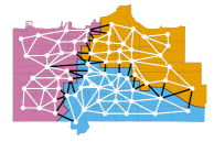
(a) The Erie graph. Edges that cross from one administrative unit to another are colored black.

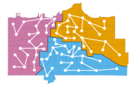
(b) Spanning trees drawn on each administrative unit.

(c) The quotient multigraph. Edges connecting boundary units in the original graphs become edges in the multigraph.

(d) The final spanning tree. A spanning tree on the quotient multigraph connects the trees on each administrative unit.

Figure 3: The two-step spanning tree sampling procedure applied to the city of Erie, Pennsylvania, with three arbitrary administrative units indicated by the colored sections of each map.

To implement this constraint, we draw the spanning trees in step (a) of Algorithm 2 in two substeps such that we sample from a specific subset of all spanning trees. First, we use Wilson’s algorithm to draw a spanning tree on each administrative unit $a\in A$, and then we connect these spanning trees to each other by drawing a spanning tree on the quotient multigraph $\widetilde{G}_{i}\,/\sim_{\eta}$. Figure 3 illustrates this process. This approach is similar to the independently-developed multi-scale merge-split algorithm of Autry et al., (2020).

Drawing the spanning trees in two steps limits the trees used to those which, when restricted to the nodes $\eta^{-1}(a)$ in any administrative unit $a$, are still spanning trees. The importance of this restriction is that cutting any edge in such a tree will either split the map exactly along administrative boundaries (if the edge is on the quotient multigraph) or split one administrative unit in two and preserve administrative boundaries everywhere else. Since the algorithm has $n-1$ stages, this limits the support of the sampling distribution to maps with no more than $n-1$ administrative splits.

The two-step construction makes clear that the total number of such spanning trees is given by

$$\tau_{\eta}(\widetilde{G}_{i})\ =\ \tau(\widetilde{G}_{i}\,/\sim_{\eta})\prod_{a\in A}\tau(\widetilde{G}_{i}\cap\eta^{-1}(a)),$$ (6)

where $\widetilde{G}_{i}\cap\eta^{-1}(a)$ denotes the subgraph of $\widetilde{G}_{i}$ which lies in unit $a$, and we take $\tau(\varnothing)=1$. Replacing $\tau$ with $\tau_{\eta}$ in the expression for the weights $w_{i}^{(j)}$ and $w^{(j)}$ then gives the modified algorithm that asymptotically samples from

$$\pi_{\eta}([\xi])\ \propto\ \exp\{-J(\xi)\}\tau_{\eta}(\xi)^{\rho}\mathbf{1}_{\{\xi\text{ connected}\}}\mathbf{1}_{\{\operatorname{dev}(\xi)\leq D\}}\mathbf{1}_{\{\operatorname{spl}(\xi)\leq n-1\}}.$$ (7)

This idea can in fact be extended to arbitrary levels of nested administrative hierarchy. We can, for example, limit not only the number of split counties but also the number of split cities and Census tracts to $n-1$ each, since tracts are nested within cities, which are nested within counties. To do so, we begin by drawing spanning trees using Wilson’s algorithm on the smallest administrative units. We then connect spanning trees into larger and larger trees by drawing spanning trees on the quotient graphs of each higher administrative level. (In this approach, cities which cross county boundaries must be split in two, and regions outside of cities must be treated as their own pseudo-city.) Even with multiple levels of administrative hierarchy, the calculation of the number of spanning trees is still straightforward, by analogy to Equation (6).

5 An Empirical Validation Study

Although the proposed algorithm has desirable theoretical properties, it is important to empirically assess its performance (Fifield et al., 2020b, ). We examine whether or not the proposed algorithm can produce a sample of redistricting maps that is actually representative of a target distribution, and how the diagnostics of Section 4.4.4 correlate with sampling accuracy.

Our validation setting is the 6-by-6 grid map shown in Figure 4. This map is small enough to obtain all possible redistricting plans with six contiguous districts using an efficient enumeration algorithm (see, e.g., Fifield et al., 2020b, ). Each precinct in the grid has an equal population. There are over 356 billion unlabeled plans with six districts, 451,206 of which have districts with exactly balanced populations. We demonstrate that the proposed algorithm can efficiently approximate a realistic target distribution on this set of balanced plans. Appendix B contains an additional validation study with four districts using a 50-precinct map taken from the state of Florida, where the population of each precinct varies.

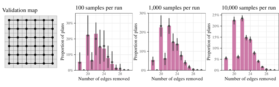
Figure 4: The 6-by-6 map used in validation (left). The remaining panels compare the distribution of the number of removed edges in the enumerated distribution (purple bars) and the sampled distribution (grey) over a number of sample sizes $S$. The dots are the mean histogram estimate across the 24 independent runs, and represent the algorithm’s bias. The vertical lines are 90% confidence intervals for the histogram estimates, and represent the sampling variability. They are calculated from the standard deviation of the estimates across the runs.

We set the target distribution by choosing $\rho=1$, which as discussed above will generate compact districts. Since this value of $\rho$ makes the proposal and sampling distributions as close as possible, the SMC algorithm will operate at peak efficiency. The validation study in Appendix B explores a wider range of values of $\rho$. As we have noted in Section 3, values of $\rho$ other than 1 may not be computationally feasible for larger redistricting problems with many more precincts.

We run Algorithm 2 on a logarithmically-spaced range of sample sizes $S$ ranging from 10 to 10,000. While $S=10$ is far too small to use in any real analysis, we include it here for illustrative purposes to demonstrate the high variability and potential bias of the algorithm when $S$ is too small. At each sample size, we perform 24 independent runs of the algorithm, each of size $S$, which allows for accurate calculation of standard errors and $\hat{R}$ for summary statistics.

To validate the algorithm, we compare the distribution of a summary statistics from each sample to the true distribution obtained by reweighting the enumerated plans according to the target measure, which is proportional to $\tau(\xi)$. The summary statistic used here is the number of edges that must be removed to form each set of districts, $\operatorname{rem}(\xi)\cdot|E(G)|$. As discussed in Section 3.3, this statistic is highly correlated with the target $\tau(\xi)$, and so is a good test of the algorithm.

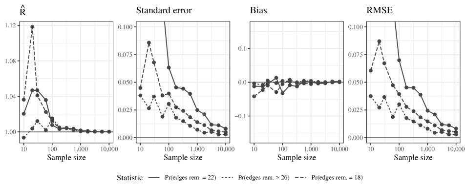
Figure 5: Convergence diagnostic $\hat{R}$ (on a log scale), standard errors, bias, and RMSE for the same three compactness summary statistics, calculated across 24 independent runs of the SMC algorithms. Values are plotted versus sample size $S$ per run.

These comparisons are summarized in the right three panels of Figure 4, which show the true distribution of the number of edges removed in purple, with the estimated histogram overlaid as solid points, for a range of sample sizes. Each histogram estimate produced by the SMC algorithm is accompanied by a 90% confidence interval produced using the standard errors calculated across the 24 independent runs (i.e., the standard deviations of the estimates for each run). With as few as $S=100$ samples, the SMC estimates are already close to the true distribution. In fact, if we tested the null hypothesis that each estimate is centered at the true value, we would only reject for one of the twelve nonzero true values at the 10% level, within the range of what would be expected by chance given the sampling variability. As the sample size increases, the variance of the SMC estimates decreases, until by $S=10,000$ samples it is mostly negligible. Overall, the agreement between the sampling and target distributions is excellent, indicating that the SMC algorithm is able to accurately sample from the target distribution in this setting.

We next study more quantitatively the quality of the SMC sample as the sample size increases, and in particular how well the diagnostics recommended in Section 4.4.4 can be used as a proxy for this quality. To do so, we focus on three particular estimands that can be obtained from the distribution of edges removed: the probability of removing exactly 22 edges (the target median; true probability 0.2328), the probability of removing exactly 18 edges (true value 0.0542), and the probability of removing more than 26 edges (true value 0.0204). The latter two statistics are especially useful as tests of the algorithm’s sampling accuracy, since they require estimating small tail probabilities which may correspond to very few redistricting plans. On the lower tail, there are just 2 possible unlabeled plans which remove exactly 18 edges, though together they comprise over 5% of the target distribution. The upper tail probability corresponds to the $p$-value a researcher would use for testing whether an enacted plan with 26 removed edges was significantly less compact than would be expected under the target distribution.

For each sample size from the SMC algorithm, we calculate the $\hat{R}$ diagnostic, and standard errors for these three summary statistics. Note that neither of these calculations requires access to the enumerated ground truth. We also compute the bias and the root mean-square error (RMSE) for the estimates, comparing to the true values from the enumerated target distribution. Ideally, the always-computable $\hat{R}$ and standard errors will well represent the generally uncomputable bias and RMSE.

Figure 5 summarizes the results of this experiment. As expected, as the SMC sample size $S$ increases, $\hat{R}$, the standard errors, and the relative RMSE also decrease. The $\hat{R}$ values fall below our recommended cutoff of 1.05 by $S=60$, indicating that for samples this large and greater, each independent run is producing similar estimates and the SMC algorithm has likely converged to the target distribution. Indeed, the estimates’ bias is closely centered around zero in this range. However, standard errors are significantly larger for the smaller sample sizes. This tracks the pattern observed in the validation above: at small sample sizes, the SMC estimates were on average unbiased for the target distribution, but had significant sampling variability.

Importantly, the calculated standard errors track the actual RMSE extremely closely, demonstrating their value as an observable proxy for this measure of sampling accuracy. In other words, with low $\hat{R}$ indicating likely algorithmic convergence (and therefore unbiasedness), the overall algorithmic error is driven almost entirely by the sampling variability, which is measurable with the standard errors.

6 Analysis of the 2011 Pennsylvania Redistricting

As discussed in Section 2, in the process of determining a remedial redistricting plan to replace the 2011 General Assembly map, the Pennsylvania Supreme Court received submissions from seven parties. In this section, we compare four of these maps to both the original 2011 plan and the remedial plan ultimately adopted by the court. We study the governor’s plan and the House Democrats’ plan; the petitioner’s plan (specifically, their “Map A”), which was selected from an ensemble of 500 plans used as part of the litigation; and the respondent’s plan, which was drawn by Republican officials.

6.1 The Setup

To evaluate these six plans, we drew reference maps from the target distribution given in Equation (7) by using the proposed algorithm along with the modifications presented in Section 4.5 to cap the number of split counties at 17 (out of a total of 67), in line with the court’s mandate. We set $\rho=1$ to put most of the sample’s mass on compact districts, and enforced $\operatorname{dev}(\xi)\leq 0.001$ to reflect the “one person, one vote” requirement.

This population constraint translates to a tolerance of around 700 people, in a state where the median precinct has 1,121 people. Like most research on redistricting, we use precincts because they represent the smallest geographical units for which election results are available. To draw from a stricter population constraint we would need to use the 421,545 Census blocks in Pennsylvania rather than the 9,256 precincts, which would significantly increase the computational burden.

6.2 Comparison with an Analogous MCMC Algorithm

We first compare the computational efficiency of the SMC algorithm with a merge-split-type MCMC algorithm (Carter et al.,, 2019; DeFord et al.,, 2021). The merge-split algorithm here uses a spanning tree-based proposal identical to the splitting procedure described in Algorithm 1: it merges adjacent districts, draws a spanning tree on the merged district, and splits it to ensure the population constraint is met. A Metropolis-Hastings correction is used, analogous to the SMC reweighting step. In fact, the implementation (contained in our open-source redist package) shares much of the same code base, which allows for performance comparisons that better reflect the different algorithmic strategies, rather than different algorithmic implementations.

The MCMC chains are each initialized with a random SMC sample, and run for 500 warm-up iterations before samples are recorded. We let the sample size vary from 100 to 4,000 for the SMC algorithm and from 100 to 8,000 for the MCMC algorithm. For each sample size, we perform four independent runs of each algorithm. The average acceptance rate for the MCMC algorithm across the four chains was 88.7%.

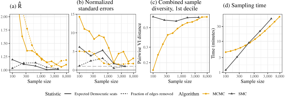
Figure 6: A comparison of sampling efficiency for SMC and MCMC algorithms using the same transition kernel. (a) Convergence diagnostic $\hat{R}$ for two summary statistics plotted against the sample size. (b) Standard errors for two statistics, normalized by the standard error for the SMC algorithm at 4,000 samples (to put the two statistics on the same scale), by sample size. (c) First decile of the pairwise variation of information distance (a measure of sample diversity) by sample size. Distance measures were computed with the combined sample of four independent runs. (d) Sampling time by sample size.

Figure 6(a) shows the $\hat{R}$ values of two summary statistics (Democratic seats and compactness) by sample size $S$ per run. By this convergence heuristic, the SMC algorithm converges more quickly, with lower $\hat{R}$ values than the MCMC algorithm for a given sample size. According to the check that $\hat{R}\leq 1.05$, the SMC algorithm has approximately converged with $S=1,600$, while the MCMC algorithm has still not converged after with than 8,000 post-warmup samples (over 7,000 unique accepted proposals), at which point the MCMC algorithm has been running 2.4 times longer than the SMC algorithm.

We find a similar story in examining the standard errors of the two statistics, which are shown in Figure 6(b) after being normalized to be on comparable scales. With four independent runs per algorithm, standard error estimates themselves are rather noisy, but the overall trend mirrors the findings for $\hat{R}$. Even at large sample sizes, the MCMC standard errors are 1.5–5 times larger than their SMC counterparts, although the MCMC standard errors are not meaningful without the underlying chains having converged.

Figure 6(c) examines the sampling efficiency from the perspective of sample diversity. As discussed in Section 4.4.4, the pairwise variation of information (VI) distance provides a way to quantify how similar the plans in each sample are to one another. If the distribution of these pairwise VI distances has a long lower tail, then there are a significant number of plans which are very similar. Figure 6(c) shows the first decile of the pairwise VI distances in the combined sample (i.e., pooled across all four runs) for each algorithm as the sample size increases. Because of the sequential nature of the MCMC algorithms, the sample diversity doesn’t match that of the SMC algorithms until there are at least 3,000 samples. This is reflected in the lag-1 autocorrelation of the MCMC sample, which was 0.982 for Democratic seats and 0.984 for compactness. Autocorrelation is of course not a direct measure of sampling efficiency, but this comparison serves to underscore the differences in the types of samples generated by each algorithm for finite sample sizes.

Figure 6(d) shows how long each algorithm takes to run for a given number of samples. Because of the fixed warm-up cost of the MCMC algorithm, it is slower than the SMC algorithm for fewer than 600 samples. Asymptotically, both algorithms have runtime linear in the number of samples. But the per-sample cost of the MCMC algorithm is lower, since only two districts are redrawn, rather than the entire map.

6.3 Compactness and County Splits

While the results of the comparison above suggest that 1,600 SMC samples is enough for Pennsylvania, we perform the rest of our analysis with 4,000 samples from one of the SMC runs. Apart from the $\hat{R}$ diagnostic examined in detail above, the other SMC diagnostics of Section 4.4.4 all indicated no problems with the generated sample.

Figures 7(a) and (b) show distribution of the fraction of edges removed $\operatorname{rem}(\xi)$ and the number of county splits $\operatorname{spl}(\xi)$ across the reference maps generated by our algorithm. The figure also shows these values for each of the six plans. The 2011 General Assembly plan is a clear outlier for both statistics, being far less compact and splitting far more counties than any of the reference plans and all of the remedial plans. Among the remedial plans, the petitioner’s is almost an outlier in being too compact, although this is perhaps not surprising—the map was generated by an algorithm explicitly designed to optimize over criteria such as population balance and compactness (Chen,, 2017). The other plans’ compactness falls within the range of the reference sample.

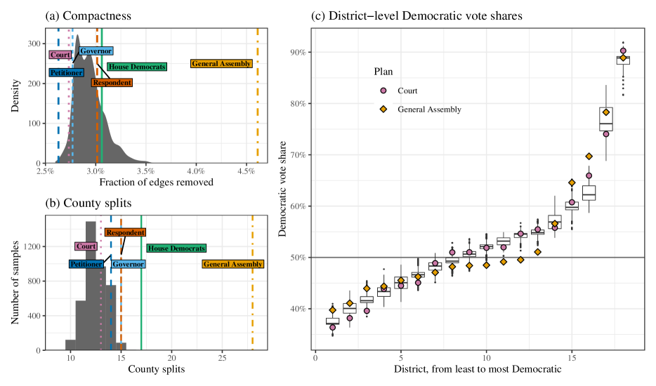
Figure 7: Summary statistics for the sampled and comparison plans: (a) compactness (smaller means more compact) and (b) county splits. Panel (c) shows the Democratic two-party vote share by district, where within each plan districts are ordered by Democratic vote share.

Figure 7(b) shows that all of the submitted remedial plans, as well as the reference sample, followed the court’s instructions to limit the number of county splits. Yet around half of the reference maps split fewer than 13 counties, the minimum number of splits found in any of the remedial plans. This may be a result of the strict population constraint (all six plans were within 1 person of equal population across all districts), or a different prioritization between the various constraints imposed.

6.4 Partisan Analysis

While important, the outlier status of the General Assembly plan as regards compactness and county splits is not sufficient to show that it is a partisan gerrymander. To evaluate the partisan implications of the six plans, we take a precinct-level baseline voting pattern and aggregate it by district to explore hypothetical election outcomes under the six plans and the reference maps. The baseline pattern is calculated by averaging the vote totals for the three presidential elections and three gubernatorial elections that were held in Pennsylvania from 2000 to 2010. These election data were also used during litigation. While being far from a perfect way to create counterfactual election outcomes, this simple averaging of statewide results is often used in academic research and courts. The values of $\hat{R}$ for the mean and various quantiles of the district-level vote shares were all within standard convergence ranges.

Then, within each plan, we number the districts by their baseline Democratic two-party vote share, so District 1 is the least Democratic and District 18 the most. Figure 7(c), analogous to Figure 7 in Herschlag et al., (2017), presents the distribution of the Democratic two-party vote share for each of the districts across the reference maps, and also shows the values for the General Assembly plan (orange triangles) and the court’s adopted plan (purple circles). When compared to the reference maps and the court’s plan, the General Assembly plan tends to yield smaller Democratic vote share in competitive districts ($p$-values of 0.0162, 0.0002, 0.0002, and 0.0002 for Districts 9–12 compared to the reference set) while giving larger Democratic vote share in non-competitive districts. The effect of this is to produce 6 Democratic seats, on average, under the General Assembly plan, compared to a range of 8–12 under the reference sample ($p$-value 0.0002) and 11 under the Court plan. All of these findings provide evidence that the General Assembly plan was gerrymandered in favor of Republicans by packing Democratic voters into non-competitive districts.

7 Concluding Remarks

Redistricting sampling algorithms allow for the empirical evaluation of a redistricting plan by generating alternative plans under a certain set of constraints. Researchers and policymakers can compute various statistics from the redistricting plan of interest and compare them with the corresponding statistics based on these sampled plans. Unfortunately, existing approaches often struggle when applied to real-world problems, owing to the scale of the problems and the number of constraints involved.

The SMC algorithm presented here can provably asymptotically sample from a specific target distribution. Because of the constructive sampling approach, it does not face the problem of potential reducibility that MCMC algorithms have, and performs more efficiently in a realistic applied setting than a MCMC algorithm that uses an identical proposal distribution. The proposed method also incorporates, by design, the common redistricting constraints of population balance, geographic compactness, and minimizing administrative splits. We expect these advantages of the SMC algorithm to meaningfully improve the reliability of outlier analysis in real-world redistricting cases.

The proposed approach has some important limitations. Like other redistricting sampling algorithms, if the target distribution strays too far from the proposal distribution, the quality of the generated sample will suffer dramatically. Close examination of diagnostic measures like $\hat{R}$, standard errors, sample diversity, and per-iteration efficiency measures like weight variance and the number of surviving plans is required to provide confidence that the algorithm is sampling accurately and has converged for particular quantities of interest. Our open-source software provides these diagnostics so that analysts can use the proposed algorithm successfully.

One important drawback particular to the SMC algorithm arises in situations with dozens or hundreds of separate districts. Like any other SMC or particle resampling scheme, as the number of iterations (districts) grows, eventually all of the samples will share a common ancestor. While this is not a problem in many SMC applications (such as Bayesian inference), for redistricting, this means that all of the sampled plans will share one or more districts that are completely identical. Any summary statistics which rely on these districts will have very large standard errors and may not converge even with a large number of samples. While this problem will be readily identified with the diagnostics we propose here, there is little the analyst can do to address the issue beyond increasing the sample size and possibly combining many independent runs of the algorithm. One interesting avenue for future research would be to examine whether several applications of an MCMC kernel at various points in the SMC algorithm could help refresh the sample and counteract the tendency to collapse to a single ancestor.

Future research should also explore the possibility of improving several design choices in the algorithm to further increase its efficiency. Wilson’s algorithm, for instance, can be generalized to sample from edge-weighted graphs. Choosing weights appropriately could lead to trees which induce maps that are more balanced or more compact. And the procedure for choosing edges to cut, while allowing for the sampling probability to be calculated, introduces inefficiencies by leading to many rejected maps. Further improvements in either of these areas should allow us to better sample and investigate redistricting plans over large maps and with even more complex sets of constraints.

Finally, we believe that the application of these sampling algorithms to real-world redistricting problems is essential. We have applied the SMC algorithm to the 2020 Congressional redistricting in all 50 states (McCartan et al.,, 2022), and this allowed us to evaluate the degree of partisan gerrymandering across states (Kenny et al.,, 2022). Such applications shed light on substantive political science theories, and highlight new methodological challenges.

Appendix A Proofs of Propositions

*

Proof.

Any spanning tree can be decomposed into two other trees and an edge joining them. Let $T\cup e\cup T^{\prime}$ denote the spanning tree obtained by joining two other spanning trees, $T$ and $T^{\prime}$, with an edge $e$. Then Equation (3) can be written as

$$q(G_{i}\mid\widetilde{G}_{i-1})=\sum_{\begin{subarray}{c}T^{(1)}\in\mathcal{T}(G_{i})\\ T^{(2)}\in\mathcal{T}(\widetilde{G}_{i})\end{subarray}}\sum_{e\in\mathcal{C}(T^{(1)},T^{(2)})}q(G_{i}\mid T^{(1)}\cup e\cup T^{(2)})\,\tau(\widetilde{G}_{i-1})^{-1}.$$

Now, $q(G_{i}\mid T^{(1)}\cup e\cup T^{(2)})$ is determined by whether whether $e^{*}=e$, i.e., if $e$ is the edge selected to be cut. If $e$ has $d_{e}$ in the top $k_{i}$ (if it induces one of the best $k_{i}$ balanced splits), then it has a $1/k_{i}$ probability of being selected in step (c) and cut. If $d_{e}$ is not in the top $k_{i}$, then this probability is zero.

Everything written to this point holds regardless of whether $G_{i}$ is a valid district (i.e., satisfies $\operatorname{pop}(V_{i})\in[P_{i}^{-},P_{i}^{+}]$). From here onwards we will restrict our attention to valid districts only. Notice that the forward-looking bounds $P_{i}^{-}$ and $P_{i}^{+}$ are stricter than merely ensuring $\operatorname{dev}(G_{i})\leq D$. That is, conditional on $\operatorname{pop}(V_{i})\in[P_{i}^{-},P_{i}^{+}]$, we must also have $\operatorname{dev}(G_{i})\leq D$.

Therefore, if a sorted edge $e_{j}$ in any spanning tree induces such a balanced partition, we must have $j\leq K_{i}$, where as in the main text $K_{i}$ counts the maximum number of such edges across all possible spanning trees. Thus, so long as we set $k_{i}\geq K_{i}$, we will have $d_{e}\leq D$.

Furthermore, across all spanning trees $T^{(1)}\in\mathcal{T}(G_{i})$ and $T^{(2)}\in\mathcal{T}(\widetilde{G}_{i})$, and connecting edges $e\in E(T^{(1)},T^{(2)})$, the value of $d_{e}$ is constant, since removing $e$ induces the same districting. Combining these two facts, we have, conditional on satisfying the bounds $P_{i}^{-}$ and $P_{i}^{+}$,

$$q(e^{*}=e\mid T^{(1)}\cup e\cup T^{(2)},\operatorname{pop}(V_{i})\in[P_{i}^{-},P_{i}^{+}])\ =\ k_{i}^{-1},$$

which does not depend on $T^{(1)}$, $T^{(2)}$, or $e$. We may therefore write the conditional sampling probability as

$$q(G_{i}\mid\widetilde{G}_{i-1},\operatorname{pop}(V_{i})\in[P_{i}^{-},P_{i}^{+}]) \ =\ \sum_{\begin{subarray}{c}T^{(1)}\in\mathcal{T}(G_{i})\\ T^{(2)}\in\mathcal{T}(\widetilde{G}_{i})\end{subarray}}\sum_{e\in\mathcal{C}(T^{(1)},T^{(2)})}\frac{1}{k_{i}\tau(\widetilde{G}_{i-1})}$$

$$\ =\ \frac{\tau(G_{i})\tau(\widetilde{G}_{i})}{\tau(\widetilde{G}_{i-1})k_{i}}|\mathcal{C}(G_{i},\widetilde{G}_{i})|,$$ (8)

where as in the main text we let $\mathcal{C}(G,H)$ represent the set of edges joining nodes in a subgraph $G$ to nodes in a subgraph $H$. ∎

* The proof proceeds by showing that the weights in Algorithm 2 are of a form derived from an existing SMC algorithm with an established central limit theorem.

Proof.

We can associate our target measure $\pi([\xi])$ on unlabeled redistricting plans with a corresponding measure on labeled plans

$$\tilde{\pi}(\xi)\coloneqq\psi([\xi])^{-1}\pi([\xi]),$$

so that the pushfoward measure obtained by mapping $\xi\mapsto[\xi]$ recovers $\pi$.

Our SMC algorithm will operate on labeled plans, targeting $\tilde{\pi}$, so that the resulting plans, when considered as representatives of their corresponding unlabeled plans, will be representative of $\pi$ in the sense given by the theorem statement. Recall that a labeled redistricting plan $\xi$ is just a tuple of graph partitions $(G_{1},G_{2},\dots,G_{n})$. We begin by extending $\tilde{\pi}(\xi)$ to a series of measures on partial plans,

$$\tilde{\pi}_{i}(G_{1},G_{2},\dots,G_{i}) :\propto\prod_{j=1}^{i}\frac{\tau(G_{j})^{\rho}\tau(\widetilde{G}_{j})}{\tau(\widetilde{G}_{j-1})}\mathbf{1}_{\operatorname{pop}(V_{j})\in[P_{j}^{-},P_{j}^{+}]}$$

$$\propto\tau(\widetilde{G}_{j})\prod_{j=1}^{i}\tau(G_{j})^{\rho}\mathbf{1}_{\operatorname{pop}(V_{j})\in[P_{j}^{-},P_{j}^{+}]},$$

for $1\leq i\leq n-2$, and where we have simplified the telescoping product in the second equality. Recall that the $\widetilde{G}_{i}$ are determined completely by $G_{1},G_{2},\dots,G_{i}$.

For $i=n-1$, the above definition would yield

$$\tilde{\pi}_{n-1}(G_{1},G_{2},\dots,G_{i})\propto\tau(\widetilde{G}_{n-1})\prod_{j=1}^{n-1}\tau(G_{j})^{\rho}\mathbf{1}_{\operatorname{pop}(V_{j})\in[P_{j}^{-},P_{j}^{+}]},=\tau(\xi)\tau(G_{n})^{1-\rho}\mathbf{1}_{\operatorname{dev}(\xi)\leq D},$$

which is close to but not quite the target measure. So we instead define $\pi_{n-1}\coloneqq\tilde{\pi}$; i.e., we add the additional terms $\exp(-J(\xi))$ and $\psi([\xi])$ and adjust for $\tau(G_{n})^{1-\rho}$.

With these partial-plan measures defined, notice that the incremental weight $w_{i}^{(j)}$ for partial plans with $1\leq i\leq n-2$ and $\operatorname{pop}(V_{j})\in[P_{j}^{-},P_{j}^{+}]$ may be written as

$$w_{i}^{(j)} =\tau(G_{i}^{(j)})^{\rho-1}\frac{k_{i}}{|\mathcal{C}(G_{i}^{(j)},\widetilde{G}_{i}^{(j)})|}$$

$$=\frac{\tau(G_{i}^{(j)})^{\rho}\tau(\widetilde{G}_{i}^{(j)})}{\tau(\widetilde{G}_{i-1}^{(j)})}\quantity(\frac{\tau(G_{i}^{(j)})\tau(\widetilde{G}_{i}^{(j)})}{\tau(\widetilde{G}_{i-1}^{(j)})}\frac{|\mathcal{C}(G_{i}^{(j)},\widetilde{G}_{i}^{(j)})|}{k_{i}})^{-1}$$

$$=\frac{\tilde{\pi}_{i}(G_{1},\dots,G_{i})}{\tilde{\pi}_{i-1}(G_{1},\dots,G_{i-1})q(G_{i}\mid\widetilde{G}_{i-1},\operatorname{pop}(V_{i})\in[P_{i}^{-},P_{i}^{+}])}.$$ (9)

For the final weighting at split $i=n-1$, the incremental weight (i.e., not including the residual previous weights $\quantity(\prod_{i=1}^{n-2}w_{i}^{(j)})^{1-\alpha}$ given by step (c) of Algorithm 2 is

$$\exp(-J(\xi^{(j)})) w_{n-1}^{(j)}\psi([\xi])^{-1}\quantity(\tau(G_{n-1}^{(j)}))^{\rho-1}$$

$$=\frac{\tilde{\pi}_{n-1}(G_{1},\dots,G_{n-1})}{\tilde{\pi}_{n-2}(G_{1},\dots,G_{n-2})q(G_{n-1}\mid\widetilde{G}_{n-2},\operatorname{pop}(V_{n-1})\in[P_{n-1}^{-},P_{n-1}^{+}])},$$

since this weight includes exactly the same additional terms as $\tilde{\pi}_{n-1}$ mentioned above. So in fact Equation (9) holds for all $1\leq i\leq n-1$.

These incremental weights are precisely those of the SMC partial rejection control algorithm of Peters et al., (2012) (see also LeGland and Oudjane, (2005)), with the weights set to zero for invalid samples and the partial rejection threshold set to the minimum possible nonzero weight. So after pushing forward to unlabeled plans, we gain immediately the theorem proved in that work (its Equation 6), viz., that for all measurable $h$ on unlabeled plans and as $S\to\infty$, we have

$$\sqrt{S}\quantity(\operatorname{\mathbb{E}}_{\pi_{S}}[h([\xi])]-\operatorname{\mathbb{E}}_{\pi}[h([\xi])])\xrightarrow{\,d\,}\mathcal{N}\quantity(0,V_{\text{SMC}}(h)),$$

for asymptotic variance $V_{\text{SMC}}(h)$ given by Equation 7 of the same work. ∎

Appendix B Additional Validation Example

This section reports the results of another validation study applied to a 50-precinct map taken from the state of Florida. As in Section 5, we use the efficient enumeration algorithm of Fifield et al., 2020b to obtain all possible redistricting maps with three and four contiguous districts, and use these plans as a baseline to validate the proposed algorithm. The left plot of Figure B.1 below shows the validation map.

Figure B.1: The 50-precinct Florida map used for validation (left) and the joint distribution of Republican dissimilarity and compactness on the map over all partitions into four districts with $\operatorname{dev}(\xi)\leq 0.10$ (right).

There are 112,515,494 partitions of the map into four districts, 33,635 of which have $\operatorname{dev}(\xi)\leq 0.10$. We evaluate the accuracy of the proposed algorithm, and compare it to the same MCMC algorithm used in Section 6, across a range of target distributions, with $\rho$ running from 0.8 to 1.2 The right plot of Figure B.1 shows the joint distribution of compactness and the summary statistic we use for the validation, the Republican dissimilarity index (Massey and Denton,, 1988). With this validation map, Republican dissimilarity is reasonably sensitive to the compactness of districts. This makes dissimilarity a good test statistic for comparing distributions that differ primarily in their average compactness.

Figure B.2: Quantile-quantile plots for 1,500 MCMC and SMC samples of Republican dissimilarity across a range of target distributions with different compactness parameters $\rho$.

For each target distribution, we sample 1,500 redistricting plans from both the SMC and MCMC algorithms, and repeat the sampling four times in order to produce $\hat{R}$ estimates. The MCMC algorithm is initialized with a random SMC-drawn map and first run for 500 warm-up iterations. To validate and compare the samples, we reweight the enumerated redistricting plans by $\tau(\xi)^{\rho}$, and then produce quantile-quantile plots of the Republican dissimilarity index, which are shown in Figure B.2.

Across the range of $\rho$ values, the agreement between the SMC sample and target distributions is excellent, even in the lower tail. The $\hat{R}$ values for the SMC algorithm were also all less than 1.003. The MCMC algorithm fares well in general but has noticeable bias for $\rho=0.9$ and $\rho=1.2$, and has some additional misses for the other target distributions as well, which manifest as small protuberances in the quantile-quantile plot. The $\hat{R}$ values for the MCMC algorithm were all less than 1.004, indicating that the overall location and scale of the Republican dissimilarity were estimated well, but $\hat{R}$ is not designed to capture these smaller-scale deviations from the target distribution.

Here and in Section 5, we validated and compared the SMC and MCMC algorithms with several summary statistics. This reflects the applied use case for redistricting analysis. But it is also informative to study how well the SMC algorithm can target the actual distribution of plans themselves. Of course, we cannot expect the algorithm to perform well in this regard if there are fewer samples then there are plans, which is the case in almost all real-world problems. So we subset the enumerated plans to those with $\operatorname{dev}(\xi)\leq 0.01$, of which there are just 38. We first generate 10,000 samples from the SMC algorithm, targeting a distribution with $\rho=1$. We measure the discrepancy between the sampled distribution of the 38 plans and the enumerated set weighted to $\tau(\xi)$ with the total variation distance, which is 0.0178 for this sample. Increasing the sample size to 50,000 decreases the total variation distance to 0.0149.

Appendix C Algorithm Implementation Details

C.1 Estimating $K_{i}$

A natural approach to estimating $K_{i}$ is to draw a moderate number of spanning trees $\mathcal{T}_{i}\subseteq\mathcal{T}(\widetilde{G}_{i})$ and compute $ok(T)$ for each $T\in\mathcal{T}_{i}$. The sample maximum, or the sample maximum plus some small buffer amount, would then be an estimate of the true maximum $\widehat{K}_{i}$ and an appropriate choice of $k_{i}$. In practice, we find little noticeable loss in algorithmic accuracy even if $k_{i}<K_{i}$. The following proposition theoretically justifies this finding. As above, $d_{e}$ represents the population deviation of the district induced by removing edge $e$ from a spanning tree.

Proposition 1.

The probability $q(e=e^{*}\mid\mathcal{F})$, i.e., the probability that an edge $e$ is selected to be cut at iteration $i$, given that the tree $T$ containing $e$ has been drawn, and that $e$ would induce a valid district, satisfies

$$\max\quantity{0,q(d_{e}\leq d_{e_{k_{i}}}\mid\mathcal{F})\quantity(1+\frac{1}{k_{i}})-1}\leq q(e=e^{*}\mid\mathcal{F})\leq\frac{1}{k_{i}},$$

where $\mathcal{F}$ is the $\sigma$-field generated by $\{T,\operatorname{pop}(V_{i})\in[P_{i}^{-},P_{i}^{+}]\}$.

Proof.

We can write

$$q(e=e^{*}\mid\mathcal{F})\ =\ q(e=e^{*},d_{e}\leq d_{e_{k_{i}}}\mid\mathcal{F})\ =\ \frac{1}{k_{i}}q(d_{e}\leq d_{e_{k_{i}}}\mid\mathcal{F}),$$

This holds because the edge $e$ will not be cut unless $d_{e}\leq d_{e_{k_{i}}}$, i.e., if $e$ is among the top $k_{i}$ edges. We then have immediately that $q(e=e^{*}\mid\mathcal{F})\leq k_{i}^{-1}$. Additionally, using the lower Fréchet inequality, we find the lower bound

$$q(e=e^{*}\mid\mathcal{F})\ =\ q(e=e^{*},d_{e}\leq d_{e_{k_{i}}}\mid\mathcal{F})$$

$$\geq\ \max\quantity{0,q(e=e^{*}\mid\mathcal{F})+q(d_{e}\leq d_{e_{k_{i}}}\mid\mathcal{F})-1}$$

$$=\ \max\quantity{0,\frac{1}{k_{i}}q(d_{e}\leq d_{e_{k_{i}}}\mid\mathcal{F})+q(d_{e}\leq d_{e_{k_{i}}}\mid\mathcal{F})-1}$$

$$=\ \max\quantity{0,q(d_{e}\leq d_{e_{k_{i}}}\mid\mathcal{F})\quantity(1+\frac{1}{k_{i}})-1}.\qed$$

If $k_{i}\geq K_{i}$, then $q(e=e^{*}\mid\mathcal{F})$ is exactly $k_{i}^{-1}$, a fact which is used in the proof of Proposition 4.2. This result, which is proved using a simple Fréchet bound, shows that as long as $q(d_{e}\leq d_{e_{k_{i}}}\mid\mathcal{F})$ is close to 1, using $k_{i}^{-1}$ in Proposition 4.2 is a good approximation to the true sampling probability.

Having sampled $\mathcal{T}_{i}$, we can compute for each value of $k$ the sample proportion of trees where a randomly selected edge $e$ among the top $k$ of edges of the tree is also among the top $k$ for the other trees—in effect estimating $q(d_{e}\leq d_{e_{k_{i}}}\mid\mathcal{F})$. We may then choose $k_{i}$ to be the smallest $k$ for which this proportion exceeds a pre-set threshold (e.g., 0.99). We have found that this procedure, repeated at the beginning of each sampling stage, efficiently selects $k_{i}$ without compromising the ability to sample from the target distribution.

C.2 Calculating $\psi([\xi])$

To calculate $\psi([\xi])$, we first observe that sequentially valid labelings of a particular unlabeled plan are in bijective correspondence with certain increasing sequences of connected subgraphs of the quotient graph $G/\xi$. Specifically, as noted in the text, for every $1\leq i\leq n-1$, the subgraph $A_{i}\coloneqq\{i+1,i+2,\dots,n\}$ of $G/\xi$ is connected if and only if $\xi$ is a sequentially valid labeling. Let $j=n-i$; then the sequence $A_{j}$ is increasing. Going from $A_{j}$ to $A_{j+1}$ for any $j$ involves adding a vertex in $G/\xi$ which is adjacent to $A_{j}$. This fact provides an easy scheme to generate the number of sequentially valid labelings: for each vertex $v$ in $G/\xi$, let $A_{1}=\{v\}$. Then pick a neighbor of $A_{1}$ and add it to the set to form $A_{2}$. Continue in this fashion until $A_{n-1}$ contains all but one vertex of $G/\xi$. Undoing our bijection, this remaining vertex is labeled 1; the vertex added between $A_{n-2}$ and $A_{n-1}$ is labeled 2, and so on.

Figure C.3 illustrates this scheme on district-level graph for the Pennsylvania court-imposed plan. We pick an arbitrary vertex, denoted by “A” in Figure C.3(a). Then we pick a neighbor, denoted “B,” and add it to the subgraph. We continue this way, adding the vertices indicated by the alphabetical ordering, until we have covered the whole district-level graph. Then the last vertex added, “R,” is labeled 1 in the district labeling, as shown in Figure C.3(b). Vertex “Q” is labeled 2, and so on, until vertex “A” is labeled 18. One can easily check that this labeling is sequentially valid—at every point, the region of the map corresponding to unlabeled districts is contiguous.

Figure C.3: Schematic of the process to generate a sequentially valid labeling, using the district-level graph for the Pennsylvania court-imposed plan. Subgraphs are built in alphabetical order in panel (a): $\{A\},\{A,B\},\dots,\{A,B,\dots,Q\}$. This corresponds to a sequentially valid labeling shown in panel (b).

As Section 4.4.2 mentioned, we adopt different strategies for calculating $\psi([\xi])$ when $n\leq 13$ and $n>13$. When there are no more than 13 districts, we simply recurse down the tree of possibilities for generating all sequentially valid plans. In the example of Figure C.3, we have 18 options for the first vertex in the subgraph. Once we have picked vertex “A”, then we could add “B” or “C”. If we add “B”, then we could add “C”, “D”, or “G”.

Clearly this tree grows quite large very quickly. Fortunately, there are many duplicate nodes—in our example, adding vertex $B$ and then $C$ in sequence produces the same subgraph as if we had added $C$ and then $B$. Thus by memoizing our counting function we can significantly reduce the number of tree branches we must explore in full.

When $n>13$, it is no longer computationally feasible to perform the recursion for each sampled plan in what will often be a large number of sampled plans. In these cases (it should be noted that for the 2020 redistricting cycle, only nine states had more than 13 districts), we can only estimate the number of sequentially valid labelings. To do so, we generate a large number of random sequentially valid labelings by following the scheme outlined above, picking vertices of $G/\xi$ to add to each $A_{j}$ uniformly at random. Since we observe the number of candidate vertices to add at each stage, and because each set of choices produces a unique sequentially valid labeling, we can compute the probability of drawing each sequentially valid labeling directly.

Denote the probability distribution created by this sampling scheme by $p_{\text{sv}}$, and the (not-probability) measure which assigns mass 1 to all $n!$ relabelings by $\mu_{\text{all}}$. Our goal here is to estimate

$$\int\mathbf{1}\{\sigma\text{ is sequentially valid}\}\differential\mu_{\text{all}}(\sigma)$$

the total number of sequentially valid labelings. This can be done with our sample from $p_{\text{sv}}$, since it is supported on precisely the same set for which the indicator function takes a value of 1. We need only take the mean of the inverse of the probability of each sampled labeling.

This importance sampling estimate is quite accurate, since the proposal support matches the target support exactly, and there is not too much variation in the proposal probabilities. The estimate can be made arbitrarily good by increasing the number of importance samples. This is demonstrated in Figure C.4, which shows how the bias in importance sampling estimates varies with the number of importance samples and the overall size of the district-level graph. In our software, we use on the order of 1,500 samples for $n=14$ by default, and more when $n$ is larger (e.g., around 3,000 for the $n=28$ Florida congressional districts). These numbers are chosen to ensure that the relative standard error (also known as the coefficient of variation) of the $\psi([\xi])$ estimate is controlled to a reasonable amount, something we demonstrate next for the case of Pennsylvania.

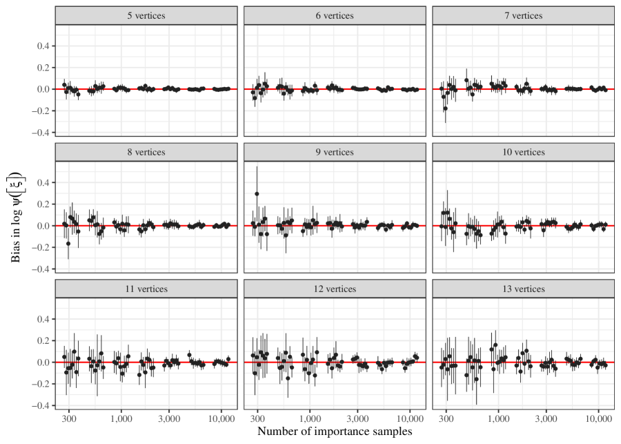
Figure C.4: Bias in importance sampling estimates of $\log\psi([\xi])$ by the number of importance samples and the number of vertices in the district-level graph. District-level graphs were selected as random subsets of the graph shown in C.3. Eight replicate experiments were performed for each importance sample size and graph size. The vertical bars for each point span two standard errors in either direction. Standard errors were calculated with the delta method.

For the district-level graph shown above in C.3, we have $\log\psi([\xi])=29.999$, calculated exactly using the recursive procedure described above. Using the importance sampling procedure with 2,000 samples, we estimate a value of $29.949$. This corresponds to a relative error of 0.051. We can also calculate the relative standard error of this example estimate with the delta method, which yields 0.052. In other words, the importance sampling error in the estimate of $\psi([\xi])$ is on the order of 5%. This is also small on the scale of the variation in $\psi([\xi])$ across plans: for the six comparison plans used in the main text, $\log\psi([\xi])$ ranges from 28.456 to 30.317. So the error in the importance sampling estimate ($|29.949-29.999|=0.05$) is just 2.7% of the range of $\log\psi([\xi])$ across these six plans.

Finally, we note that the procedures used here to calculate $\psi([\xi])$ can also be applied to partial plans. Notating this formally is more difficult, but a partial plan can be viewed as a (unbalanced) plan with fewer districts. Calculating $\psi$ for these partial plans and incorporating them into the SMC weights in Algorithm 2 improves the sampling efficiency without changing the target distribution, as long as each partial $\psi$’s contribution to the weights is canceled in the following iteration. This is the approach taken by our software implementation.

C.3 Stabilizing Importance Weights

When $\rho\neq 1$ or when the constraints imposed by $J$ are severe, there can be substantial variance in the importance sampling weights. For large maps with $\rho=0$, for instance, the weights will generally span hundreds if not thousands of orders of magnitude. This reflects the general computational difficulty in sampling uniformly from constrained graph partitions. As Najt et al., (2019) show, sampling of node-balanced graph partitions is computationally intractable in the worst case. In such cases, the importance sampling estimates will be highly variable, and resampling based on these weights may lead to degenerate samples with only one unique map.

When the importance weights are variable but not quite so extreme, we find it useful to truncate the normalized final weights (such that their mean is 1) from above at a value $w_{\max}$ at the end of sampling. The theoretical basis for this maneuver is provided by Ionides, (2008), who proved that as long as $w_{\max}\to\infty$ and $w_{\max}/S\to 0$ as $S\to\infty$, the resulting estimates are consistent and have bounded variance (since the truncation occurs only after the final SMC step, these conclusions, which were made in the context of importance sampling, carry over.) One such choice we have found to work well for the weights generated by this sampling process is $w_{\max}=S^{0.4}/100$, though for particular maps other choices of exponent and constant multiplier may be superior.

Truncation is no panacea, however. As with any method that relies on importance sampling, it is critical to examine the distribution of importance weights to ensure that they will yield acceptable resamples.

C.4 Computational Complexity

The two asymptotically slowest steps of the SMC algorithm are computing $\tau(G_{i})$ for every district $G_{i}$ and drawing a spanning tree using Wilson’s algorithm for each iteration. All other steps, such as computing $d_{e}$ and $|\mathcal{C}(G_{i}^{(j)},\widetilde{G}_{i}^{(j)})|$, are linear in the number of vertices, and are repeated at most once per iteration. Computing $\tau(G_{i})$ requires computing a determinant, which currently has computational complexity $O(|V_{i}(\xi)|^{2.373})$ though most implementations are $O(|V_{i}(\xi)|^{3})$. Since this must be done for each district of size roughly $m/n$, the total complexity for sampling one plan is $O(n\cdot(m/n)^{2.373})$. For the spanning trees, the expected runtime of Wilson’s algorithm is the mean hitting time of the graph, which is $O(m^{2})$ in the worst case. So the total complexity for each sample is roughly $O(nm^{2}+m^{2.373}n^{-1.373})$ (ignoring the random rejection procedure). Note that when $\rho=1$, we need not compute $\tau(G_{i})$, and the total complexity is roughly $O(nm^{2})$.

References

- Akitaya et al., (2022) Akitaya, H. A., Korman, M., Korten, O., Souvaine, D. L., and Tóth, C. D. (2022). Reconfiguration of connected graph partitions via recombination. Theoretical Computer Science.
- Autry et al., (2020) Autry, E., Carter, D., Herschlag, G., Hunter, Z., and Mattingly, J. (2020). Multi-scale merge-split Markov chain Monte Carlo for redistricting. Working paper.
- Bangia et al., (2017) Bangia, S., Graves, C. V., Herschlag, G., Kang, H. S., Luo, J., Mattingly, J. C., and Ravier, R. (2017). Redistricting: Drawing the line. arXiv preprint arXiv:1704.03360.
- Bozkaya et al., (2003) Bozkaya, B., Erkut, E., and Laporte, G. (2003). A tabu search heuristic and adaptive memory procedure for political districting. European journal of operational research, 144(1):12–26.
- Cannon et al., (2022) Cannon, S., Duchin, M., Randall, D., and Rule, P. (2022). Spanning tree methods for sampling graph partitions. arXiv preprint arXiv:2210.01401.
- Carter et al., (2019) Carter, D., Herschlag, G., Hunter, Z., and Mattingly, J. (2019). A merge-split proposal for reversible Monte Carlo Markov chain sampling of redistricting plans. arXiv preprint arXiv:1911.01503.
- Chatterjee and Diaconis, (2018) Chatterjee, S. and Diaconis, P. (2018). The sample size required in importance sampling. The Annals of Applied Probability, 28(2):1099–1135.
- Chen, (2017) Chen, J. (2017). Expert report of Jowei Chen, Ph.D. Expert witness report in League of Women Voters v. Commonwealth.
- Chen and Rodden, (2013) Chen, J. and Rodden, J. (2013). Unintentional gerrymandering: Political geography and electoral bias in legislatures. Quarterly Journal of Political Science, 8(3):239–269.
- Chikina et al., (2017) Chikina, M., Frieze, A., and Pegden, W. (2017). Assessing significance in a Markov chain without mixing. Proceedings of the National Academy of Sciences, 114(11):2860–2864.
- Chikina et al., (2019) Chikina, M., Frieze, A., and Pegden, W. (2019). Understanding our Markov Chain significance test: A reply to Cho and Rubinstein-Salzedo. Statistics and Public Policy, 6(1):50–53.
- Cho and Liu, (2018) Cho, W. K. T. and Liu, Y. Y. (2018). Sampling from complicated and unknown distributions: Monte Carlo and Markov chain Monte Carlo methods for redistricting. Physica A: Statistical Mechanics and its Applications, 506:170–178.
- Cho and Rubinstein-Salzedo, (2019) Cho, W. K. T. and Rubinstein-Salzedo, S. (2019). Understanding significance tests from a non-mixing Markov Chain for partisan gerrymandering claims. Statistics and Public Policy, 6(1):44–49.
- Cirincione et al., (2000) Cirincione, C., Darling, T. A., and O’Rourke, T. G. (2000). Assessing South Carolina’s 1990s congressional districting. Political Geography, 19(2):189–211.
- Cover and Thomas, (2006) Cover, T. M. and Thomas, J. A. (2006). Elements of information theory. John Wiley & Sons, 2nd edition.
- DeFord et al., (2021) DeFord, D., Duchin, M., and Solomon, J. (2021). Recombination: A family of Markov chains for redistricting. Harvard Data Science Review. https://hdsr.mitpress.mit.edu/pub/1ds8ptxu.
- Del Moral et al., (2006) Del Moral, P., Doucet, A., and Jasra, A. (2006). Sequential monte carlo samplers. Journal of the Royal Statistical Society: Series B (Statistical Methodology), 68(3):411–436.
- Doucet et al., (2001) Doucet, A., de Freitas, N., and Gordon, N. (2001). Sequential Monte Carlo methods in practice. Springer, New York.
- Dube and Clark, (2016) Dube, M. P. and Clark, J. T. (2016). Beyond the circle: Measuring district compactness using graph theory. In Annual Meeting of the Northeastern Political Science Association.
- Duchin, (2018) Duchin, M. (2018). Outlier analysis for Pennsylvania congressional redistricting.
- (21) Fifield, B., Higgins, M., Imai, K., and Tarr, A. (2020a). Automated redistricting simulation using Markov chain Monte Carlo. Journal of Computational and Graphical Statistics, 29(4):715–728.
- (22) Fifield, B., Imai, K., Kawahara, J., and Kenny, C. T. (2020b). The essential role of empirical validation in legislative redistricting simulation. Statistics and Public Policy, 7(1):52–68.
- Gelman et al., (2013) Gelman, A., Carlin, J. B., Stern, H. S., Dunson, D. B., Vehtari, A., and Rubin, D. B. (2013). Bayesian data analysis.
- Gelman and Rubin, (1992) Gelman, A. and Rubin, D. B. (1992). Inference from iterative simulation using multiple sequences. Statistical science, 7(4):457–472.
- Guth et al., (2020) Guth, L., Nieh, A., and Weighill, T. (2020). Three applications of entropy to gerrymandering. arXiv preprint arXiv:2010.14972.
- Herschlag et al., (2017) Herschlag, G., Ravier, R., and Mattingly, J. C. (2017). Evaluating partisan gerrymandering in Wisconsin. arXiv preprint arXiv:1709.01596.
- Ionides, (2008) Ionides, E. L. (2008). Truncated importance sampling. Journal of Computational and Graphical Statistics, 17(2):295–311.
- Kenny et al., (2020) Kenny, C. T., McCartan, C., Fifield, B., and Imai, K. (2020). redist: Computational algorithms for redistricting simulation. https://CRAN.R-project.org/package=redist.
- Kenny et al., (2022) Kenny, C. T., McCartan, C., Simko, T., Kuriwaki, S., and Imai, K. (2022). Widespread partisan gerrymandering mostly cancels nationally, but reduces electoral competition. arxiv preprint arXiv:2208.06968.
- Kostochka, (1995) Kostochka, A. V. (1995). The number of spanning trees in graphs with a given degree sequence. Random Structures & Algorithms, 6(2-3):269–274.
- League of Women Voters v. Commonwealth, (2018) League of Women Voters v. Commonwealth (2018). 178 A. 3d 737 (Pa: Supreme Court).
- Lee and Whiteley, (2018) Lee, A. and Whiteley, N. (2018). Variance estimation in the particle filter. Biometrika, 105(3):609–625.
- LeGland and Oudjane, (2005) LeGland, F. and Oudjane, N. (2005). A sequential particle algorithm that keeps the particle system alive. In 2005 13th European Signal Processing Conference, pages 1–4. IEEE.
- Liu et al., (2001) Liu, J. S., Chen, R., and Logvinenko, T. (2001). A theoretical framework for sequential importance sampling with resampling. In Sequential Monte Carlo methods in practice, pages 225–246. Springer.
- Liu et al., (1998) Liu, J. S., Chen, R., and Wong, W. H. (1998). Rejection control and sequential importance sampling. Journal of the American Statistical Association, 93(443):1022–1031.
- Liu et al., (2016) Liu, Y. Y., Cho, W. K. T., and Wang, S. (2016). PEAR: a massively parallel evolutionary computation approach for political redistricting optimization and analysis. Swarm and Evolutionary Computation, 30:78–92.
- Macmillan, (2001) Macmillan, W. (2001). Redistricting in a GIS environment: An optimisation algorithm using switching-points. Journal of Geographical Systems, 3(2):167–180.
- Magleby and Mosesson, (2018) Magleby, D. B. and Mosesson, D. B. (2018). A new approach for developing neutral redistricting plans. Political Analysis, 26(2):147–167.
- Massey and Denton, (1988) Massey, D. S. and Denton, N. A. (1988). The dimensions of residential segregation. Social forces, 67(2):281–315.
- Mattingly and Vaughn, (2014) Mattingly, J. C. and Vaughn, C. (2014). Redistricting and the will of the people. arXiv preprint arXiv:1410.8796.
- McCartan et al., (2022) McCartan, C., Kenny, C. T., Simko, T., Garcia III, G., Wang, K., Wu, M., Kuriwaki, S., and Imai, K. (2022). Simulated redistricting plans for the analysis and evaluation of redistricting in the united states. Scientific Data, 9(1):689.
- McKay, (1981) McKay, B. D. (1981). Spanning trees in random regular graphs. In Proceedings of the Third Caribbean Conference on Combinatorics and Computing. Citeseer.
- Mehrotra et al., (1998) Mehrotra, A., Johnson, E. L., and Nemhauser, G. L. (1998). An optimization based heuristic for political districting. Management Science, 44(8):1100–1114.
- Najt et al., (2019) Najt, L., Deford, D., and Solomon, J. (2019). Complexity and geometry of sampling connected graph partitions. arXiv preprint arXiv:1908.08881.
- National Conference of State Legislatures, (2021) National Conference of State Legislatures (2021). Redistricting criteria. Available at https://www.ncsl.org/research/redistricting/redistricting-criteria.aspx.
- Olsson and Douc, (2019) Olsson, J. and Douc, R. (2019). Numerically stable online estimation of variance in particle filters. Bernoulli, 25(2):1504–1535.
- Peters et al., (2012) Peters, G. W., Fan, Y., and Sisson, S. A. (2012). On sequential monte carlo, partial rejection control and approximate bayesian computation. Statistics and Computing, 22(6):1209–1222.
- Polsby and Popper, (1991) Polsby, D. D. and Popper, R. D. (1991). The third criterion: Compactness as a procedural safeguard against partisan gerrymandering. Yale Law & Policy Review, 9(2):301–353.
- Tutte, (1984) Tutte, W. T. (1984). Graph Theory. Addison-Wesley.
- Vehtari et al., (2019) Vehtari, A., Gelman, A., Simpson, D., Carpenter, B., and Bürkner, P.-C. (2019). Rank-normalization, folding, and localization: An improved r for assessing convergence of mcmc. arxiv. arXiv preprint arXiv:1903.08008.
- Wilson, (1996) Wilson, D. B. (1996). Generating random spanning trees more quickly than the cover time. In Proceedings of the twenty-eighth annual ACM symposium on Theory of computing, pages 296–303.
- Wu et al., (2015) Wu, L. C., Dou, J. X., Sleator, D., Frieze, A., and Miller, D. (2015). Impartial redistricting: A Markov Chain approach. arXiv preprint arXiv:1510.03247.