An estimator for predictive regression:
reliable inference for financial economics††thanks: Thanks to Isaiah Andrews, Joseph Blitzstein, Andrew Patton, Ashesh
Rambachan, Julia Shephard and particularly Jihyun Kim and Nour Meddahi. The
code which produces all the simulation results is in sign1.r. The
code which produces all the empirical results (including downloading the
data) is in RegFinance1.r and Recursive1.r.
Abstract
Estimating linear regression using least squares and reporting robust standard errors is very common in financial economics, and indeed, much of the social sciences and elsewhere. For thick tailed predictors under heteroskedasticity this recipe for inference performs poorly, sometimes dramatically so. Here, we develop an alternative approach which delivers an unbiased, consistent and asymptotically normal estimator so long as the means of the outcome and predictors are finite. The new method has standard errors under heteroskedasticity which are easy to reliably estimate and tests which are close to their nominal size. The procedure works well in simulations and in an empirical exercise. An extension is given to quantile regression.
Keywords: Median; Prediction; Quantile; Quantile regression; Regression; Robustness; Robust standard errors; Tails.
1 Introduction
Think about an outcome variable and predictors . Throughout assume and exist (meaning and ). Write , where T denotes a transpose, then . I will work with a linear in parameters “predictive regression,”
| (1) |
is my estimand and inference about is my goal.
The motivation for this paper is that thick tailed predictors with heteroskedastic outcomes are very common in financial economics. Finance researchers nearly always assume that the mean of asset returns exists, while the vast bulk believe the variance exists. Due to the empirical evidence of their sample instability and the results from applying extreme value theory to estimate the data’s tail index, many are skeptical that third or fourth moments exist (e.g. the accessible review of Cont (2001)). This challenges traditional least squares based “robust standard errors” type inference methods nearly universally used in financial economics, which rely on these higher order moments for their justification. This credibility gap rarely impacts the way applied researchers behave, perhaps understandably so because it is less than clear what action to take without potentially employing quite complicated methods. This paper provides a simple solution to this problem.
More broadly, the use of traditional least squares based robust standard errors is very common in many areas of applied statistics (e.g. see the beginning of King and Roberts (2015) for a discussion of the use in political science and MacKinnon (2012) for a discussion of the econometrics literature). The methods developed here could prove useful in other applied fields, for thick tailed data is very common, although often less apparent than in the data rich environment of financial economics.
The core of this paper focuses on the sample , a sequence of pairs of i.i.d. random variables which each obeys (1), highlighting
The presence of reduces the influence of thick tailed predictors, making valid inference possible for problems in financial economics. Downweighting extreme predictors is at the heart of the “bounded-influence function” part of the robustness literature. A classic reference to that work is Krasker and Welsch (1982). My focus is on the contribution can make to allowing valid inference about under heteroskedasticity.
Then
so, if the symmetric is invertible, then
Crucially
which will drive the robustness of to thick tailed predictors.
will be conditionally (on the predictors) unbiased, consistent, asymptotically normal with a variance which can be estimated by
| (2) |
where , so long as and . In practice I take , so the truncation is irrelevant except for the most extraordinary predictors. Without the truncation we need the additional condition that .
In comparison, Assumption 4 of White (1980) spells out that Eicker (1967), Huber (1967) and White (1980) robust standard errors needs for inference on based on least squares
to be asymptotically valid. Recall these standard errors are based on
Unfortunately, financial economists may well not have those four moments available to them. Monte Carlo and empirical results presented later will demonstrate this asymptotic worry is important in practice. Further, the results suggest that even if more moments exist than four the finite sample inference is still very fragile unless is very substantial. Overall, in my opinion, the evidence suggests Eicker (1967), Huber (1967) and White (1980) type “robust standard errors” are not credible in financial economics. is one potential solution.
The same line of argument holds for inference on the -quantile regression:
The estimand is, again, . Recall the check-function notation . I advocate the estimator
noting is convex in with bounded subderivative
This is an alternative to the celebrated Koenker and Bassett (1978) estimator
which has the unbounded subderivative
When then is, famously, the least absolute deviation (LAD) estimator of Boscovich from 1805. Unfortunately, inference on is, again, not robust to thick tailed predictors and so is not, in my opinion, credible for financial economics. The math is more complicated for than , but the source of weakness is exactly the same. is one potential consistent and asymptotically normal solution. Is easy to compute? is applied to the preprocessed data and , noting
The preprocessing stabilizes statistical inference, while existing software can be used without any further changes.
The remaining parts of this paper are as follows. In Section 2 I will focus on a scalar predictor and explain where comes from and derive its main inferential properties. While doing this I will review the literature on this topic, linking results across different intellectual fields.
In Section 3 I provide conditions for identifying and derive a corresponding method of moments estimator . Section 4.1 holds the main condition properties of , conditioning on the predictors. Section 4.2 contains the corresponding unconditional properties of . In both sections is compared to the corresponding least squares estimator . Section 5 presents the results from various simulation experiments to see how effective the asymptotics guidance is.
Section 6 contains results from a massive number of hypothesis tests using , where I identify stocks with high betas or low betas. This allows me to form high (or low) beta portfolios, which is a potentially useful investment vehicle for investors unable to take on financial leverage (e.g. young savers into pensions). I also study how these procedures work as they are rolled through the time series database.
2 Why is interesting and the literature
The main virtues of are seen in the most stripped down case: the focus of this section.
Assume a linear in parameters “predictive regression”
| (3) |
for outcome and scalar predictor , where . As each item is a scalar, no bolding will be used here. Upper cases denote random variables, lower cases fixed numbers.
Then,
so
implying
where and .
I give nine features of , weaving them together with a literature review.
2.1 Ways of deriving
The first three features are different ways of deriving .
First, multiply both sides of (3) by , then
If and exist, then unconditionally
Crucially , so a sufficient condition for to exist is that . The same argument implies exists if . If, in addition, then
So a sufficient condition for to be identified is and . Let be a sequence of pairs of random variables which each obeys (3). Then
| (4) |
is a method of moments estimator. By the strong law of large numbers, under just two conditions, and ,
Hence is consistent if the data is a tad less thick tailed than, for example, Cauchy random variables.
Second, is an Instrumental Variable (IV) estimator, where the “instruments” are . Often, IV estimators behave notoriously poorly in many of their applications as the “relevance” condition of instrumental variables is “weak” (e.g. the reviews in Andrews et al. (2019)). This is not the case here, as the relevance condition should hold strongly.
Third, is the maximum quasi-likelihood (ML) estimator from the contrived model . This implies the existence of a quasi-likelihood , which downweights predictors with very large compared to the tradition homoskedastic quasi-likelihood case. invites a Gaussian prior for given the predictors, delivering a Gaussian quasi-posterior for given the outcomes and predictors.
My fourth point is different. Divide the top and bottom of (4) by and write
then the geometry of the estimator is shown in Figure 1, where the slope of the green line is . The length of horizontal red line is , while the vertical red line moves down from to .
2.2 Major properties of
The next two features are the main inferential properties of .
Fifth, in terms of conditional inference, if the pairs are independent and (3) holds for each , then , where and the observed predictors . Further, for if ,
Then can be estimated by (this will be discussed in more detail shortly). This makes inference based on the approximate pivot
effective for thick tailed heteroskedastic data. Whether the researcher assumes homoskedasticity or not does not change the form of . It was this property which initially made me interested in .
Sixth, in terms of unconditional inference, if the pairs are independent and identically distributed (i.i.d.), then the strong law of large numbers implies that, as ,
so long as and . Here, is a “pseudo-true” value of . If (3) holds, then Adam’s Law implies that and , so , forcing . Further, defining and additionally assuming , then unconditionally
hence heteroskedasticity has no impact on the limit distribution of . Further, can be estimated by . Finally, define where , so
If exists then can be consistently estimated by . More broadly, if does not exist then performs poorly in theory and in simulations (this will be reported in Sections 4.3 and 5). Instead, a weighted version, which clips the estimator for large absolute predictors, where the weight , is consistent for , requiring, again just requiring . In simulations, I take (so if then ), so the clipping will have literally no impact on nearly all applied work. However, the evidence suggests the weight is a worthwhile guardrail for very thick tailed data.
2.3 Relating to other estimators
Seventh, in the context of linear regressions for stable random variables, Blattberg and Sargent (1971) derived
regarding the predictors as non-stochastic, minimizing the -stable scale in the class of linear unbiased estimators. When , would be , but they did not cover that case, nor its analytic properties. When standard errors are not robust to heteroskedasticity. Samorodnitsky et al. (2007) studied the distributional properties of under very heavy tails in , but assuming independence between the predictors and the regression errors. This independence assumption takes them outside our interests. Gorji and Aminghafari (2019) builds on Blattberg and Sargent (1971) and Samorodnitsky et al. (2007) towards non-parametric regression.
Eighth, So and Shin (1999) studied estimating autoregressions with the instrument , yielding an estimator
To So and Shin (1999), had attractive properties in heavy tailed time series. They call this a “Cauchy estimator”, after Cauchy (1836) (who followed up his first paper with 6 others around this topic), noting that can be thought of as an instrumental variable estimator and a generalized least squares estimator. The historians of least squares and regression in statistics usually associate Cauchy’s work with numerical interpolation (e.g. Seal (1967), Ch. 13 of Farebrother (1999) and Ch. 4 of Heyde and Seneta (1977)). It matches only in the scalar case with no intercept. Heyde and Seneta (1977) detail Cauchy’s work on regression from a modern perspective. Ch. 13.5 of Linnik (1961) discusses the multivariate Cauchy’s method, proving it is unbiased and derives the variance of in the scalar case for non-stochastic predictors under homoskedasticity.
Phillips et al. (2004) generalized the So and Shin (1999) use of in an autoregression to an “instrument generating function” , where is an asymptotically homogenous function. Kim and Meddahi (2020) mention the So and Shin (1999) approach to fitting autoregressions in the context of time series of realized volatility type objects (which tend to be thick tailed). They also link to Samorodnitsky et al. (2007). Their interest was in consistent estimation for time series with heavy tailed regression errors. Ibragimov et al. (2020) look at time series estimators of type under volatility clustering.
Mikosch and de Vries (2013) studied the properties of least squares under heavy tailed predictors, providing interesting results and references. Hill and Renault (2010) devised trimming methods for the GMM which allow for both heavy tailed variables and Gaussian limit theory. Hallin et al. (2010) looked at using rank based methods in regression context with heavy tailed data, while Butler et al. (1990) use adaptive statistical models for regressions, assuming predictors and prediction errors are independent.
Ninth, more broadly, Balkema and Embrechts (2018) provides a review of a substantial literature on robust estimation and heavy tailed data, as well as comparing procedures using Monte Carlo methods. Related work is Kurz-Kim and Loretan (2014). Nolan and Ojeda-Revah (2013) looks at linear regressions with heavy tailed errors. Of course, these last two papers interface with the influential robustness literature, reviewed by Hampel et al. (2005). Sun et al. (2020) is an interesting recent paper which is close to our setup. It uses a Huber loss for a linear predictive regression where the threshold is selected adaptively so that asymptotically they still recover the estimand, the parameter indexing the predictive regression. The Sun et al. (2020) procedure is likely to be asymptotically more efficient than .
The use of
is a special case of the important wide ranging work on the bounded influence function literature, which goes back to Mallows (1975a, b) and Krasker and Welsch (1982). Most of their focus is on efficient robust estimation of (or, in particular, M-estimator generalizations). My interest is in being able to estimate the standard errors under heteroskedasticity so that inference in financial economics is reliable.
2.4 Comparing to least squares
I now compare to the ML estimator from the conditionally Gaussian linear regression ,
the celebrated “least squares” estimator. Of course, under homoskedasticity, will be more efficient than . For i.i.d. pairs, famously, if enough moments exist, then unconditionally
Then estimates . Define where, again, . Then
which needs to behave well as an estimator of , in theory and in simulations. If enough moments exist, then, taken together, this motivates robust standard errors based on , following Eicker (1967), Huber (1967) and White (1980) (where Assumption 4 spells out the need for ). Robust standard errors are used in vast numbers of applied papers. Unfortunately is a poor estimator unless (i) is very large, (ii) is known to be independent of or (iii) the predictors are thin tailed. This makes valid inference based on the asymptotic pivot
challenging for data in finance. It is well known that often has poor finite sample properties, although the infeasible version of this does not. Some try to mend this problem using a bootstrap of the approximate pivot or an Edgeworth expansion, e.g. MacKinnon and White (1985), Hall (1992), MacKinnon (2012) and Hausman and Palmer (2012).
As I said, under homoskedasticity will be more efficient than (e.g. the Gauss-Markov Theorem or, in the Gaussian outcomes case, Cramér-Rao inequality), with
by Jensen’s inequality. This point goes back at least to Ch. 13.5 of Linnik (1961). If , with equal probability, then , so is fully efficient. Of course it is, in that case, so . Under , then hence the is substantially more efficient than . Under the thicker tailed , so . If is very thick tailed, then can go to infinity in cases where is finite. Then is a much more precise estimator, on average, but the Gaussian CLT no longer holds for in cases where the CLT for is still useful. This suggests CLT for may be a more practical guide in the kind of thick tailed data often seen in finance, for example.
3 Identification and estimation of
Again, think about an outcome variable and predictors , where and . The following is enough to establish identification of .
Assumption 1 (Joint law of )
-
A1.
and . Write ,
-
A2.
There exists a single such that
(5) so all .
-
A3.
is positive definite.
As A1 includes an intercept, note that , while .
Theorem 1
Under A1,
exists and is symmetric, positive semidefinite. Under A1+A3, it is also positive definite.
Proof. so A1 implies exists. By construction, it is symmetric, positive semi-definite. Assumption A3 pushes this to positive definite. QED.
The estimand will be , while will be a “nuisance”. Using Theorem 1, the following is straightforward.
Theorem 2 (Identification)
Assume A1-A3, then
| (6) | |||||
This Theorem says that and can be uniquely determined, that is, identified, from , and . Further, and crucially, all three of these terms are guaranteed to exist if both and exist. Adding Assumption A3 is the only substantial assumption made beyond the core model A1 and A2.
Now turn to estimation.
Let be a sequence of pairs of random variables which each obeys A1-A3.
Define
Importantly, and is symmetric and positive semi-definite.
We now introduce a method of moment estimator of .
Definition 1
Assume is positive definite. Using the moment condition (6), define a method of moment estimator
is an instrumental variable (IV) estimator, that uses the as instruments (although note that is buried within ).
Example 1
If and no intercept, so , then ,
which is non-centered (prediction) version of the estimator discussed in Section 2.
It is sometimes helpful to unpack into its elements .
Theorem 3
Assume . Define the weights and weighted averages
and the weighted sums of outer products
Then
delivering the -th residual , .
Proof. Given in the Appendix.
Example 2
If then
and
4 Properties of
4.1 Conditional properties of
There are two broad ways of performing inference on the parameters that index a predictive regression: conditionally and unconditionally. First, focus on the conditional case.
Assumption 2 (Conditional assumptions)
-
B1.
The matrix
is positive definite.
-
B2.
The pairs are independent.
-
B3.
, for .
-
B4.
The matrix
is positive definite.
-
B5.
, for , where .
Write all the random predictors as and their observed version in the sample as .
Theorem 4
If B1-B2 and A1-A2 hold for each , then . If B1-B3 and A1-A2 hold, then
Further, under B1-B5, there exists a constant , such that
where denotes the set of all convex subsets of and
Proof. Given in the Appendix.
The first two results are of a familiar form. The last result is a type of Berry-Esseen bound. Although the Berry-Esseen bound looks at first sight asymptotic, it is not, it is exact. Assumption B5 is a Lyapunov-type condition. It has the asymptotic implications that under B1-B5, so as increases
The Berry-Esseen bound provides guidance if increases with (so long as and are well behaved as increases).
Remark 1
Assume is non-singular. Then Theorem 4 corresponds to the classical and
where . Assume is positive definite. The corresponding Berry-Esseen bound is
where denotes the set of all convex subsets of and
Finally,
Example 3
4.2 Unconditional inference
The corresponding result for unconditional inference is stated in Theorem 5. The proof is a straightforward application of the usual limit theory for the method of moments, thinking of the problem as a type of two step estimation problem (e.g. Newey and McFadden (1994)).
Theorem 5
Assume , a compact parameters space. Assume that the pairs are i.i.d. obeying A1-A3 and write as the true values under this sampling. Writing , and , then as , so
assuming , where .
Proof. Given in the Appendix.
Section 3 showed that the existence of and is a sufficient condition for and to both exist. Hence the central limit theory for can hold in cases where the variance of and the variance of do not exist. What is needed is the existence of the conditional variance of the outcomes given the predictors. To remove the conditional variance assumption a switch in estimand is needed, e.g. to one based on quantiles. This will be discussed in Section 7.
Remark 2
The result above compares to the classical
assuming and exist and is invertible.
Example 4
(Continuing Example 2) When , then write , recalling , so
Remark 3
The i.i.d. assumption on the sequence of pairs in Theorem 5 is not what drives the result. That assumption can be replaced by assuming the sequence is a martingale difference with respect to the sequence’s natural filtration.
4.3 Estimating the standard errors
In practice estimating or is delicate. The estimation challenge for thick tailed predictors has been understated in the applied finance literature.
Focus on the scalar predictor case with no intercept, so , to concentrate on the important ideas. Then . The extension to the general case is immediate. Then
so define
as an estimator of . Then, converges to using the strong law of large numbers as . What happens to the two other terms in the above expression?
Now, if , under the conditions of Theorem 5,
while
as long as exists (in which case ). Then, under the conditions of Theorem 5,
But what happens if does not exists? The CLT for does not change and is well behaved. However, trouble brews in the terms and . In our simulations, becomes inadequate if ceases to exist.
To entirely circumvent this problems, I use a weighted estimator, where the weights will be denoted ,
This clips regression residuals associated with large predictors. Then,
As , these three results imply that
even if does not exist.
In our simulation and empirical work we take . If , the scaled threshold is . This implies the weight function will not clip any regression residual unless the associated predictor is extraordinarily unusual. For thin tailed predictors, clipping is neither helpful or harmful. For thick tailed predictors, it is deeply important. As researchers usually do not know the tail behavior of their predictors, the safe approach is to always include the weighting function.
More broadly, the same line of argument applies to
where now , so long as . More straightforwardly, by the strong law of large numbers
so long as exists – which is true so long as exists.
Thus asymptotically valid estimators of the standard errors can be computed without needing any more assumptions about higher order moments.
As mentioned in the introduction, for least squares, their robust standard errors need at least the fourth moments of the predictors to be valid. This is spelt out in Assumption 4 of White (1980).
Example 5
5 Simulation experiment
In this section I focus on the performance of the approximate pivots
in the case with an intercept and one predictor, so , where the weight function for is , . The truncation in has no impact except for the very extreme cases we discuss in Section 5.3, which studies in the case where . Recall, theory suggests that weighting is needed in that case.
The simulation design I initially use is based around regressing stock returns on a broad based index, to estimate a “beta”. The design mimics the empirical challenge tackled in the next section. That challenge looks at 2 years of weekly percentage arithmetic returns on a major U.S. company, , and will be the S&P500 index arithmetic returns. In the empirical work this will be implemented for more than 400 individual companies, using hypothesis tests based on and to identify stocks with very high or very low betas.
5.1 Initial experiment
Assume
and
This implies that, for every value of , the , , and . The simulations will have homoskedasticity, but the approximate pivots will be computed without imposing that. Importantly if the is not asymptotically N(0,1), while will be. Hence is expected to have poor performance unless is substantially above 4. This is what you will see in the simulations.
To calibrate this using universally available data, I look at weekly arithmetic (total) returns on the SPDR S&P 500 ETF Trust (SPY) from 1st August 2018 to 4th August 2020, downloaded using the R package Quantmod from Yahoo’s database. The R code for this download, delivering a vector of weekly returns “X” is
getSymbols("SPY",from=’2018-08-01’,to=’2020-08-04’,verbose = TRUE); head(SPY);
XdataM = (to.weekly(SPY))$SPY.Adjusted
X = data.matrix(100*diff(XdataM)/lag(XdataM))[-1];
The sample mean and standard deviation suggest taking , , and the ML estimator of , computed using R’s function fitdistr for the student-t distribution, is 2.16 with a standard error of around 0.5. This is not an unusual result — typical extreme value theory estimates of the tail index of equity indexes suggest 2 but not 4 moments exist.
To nudge towards safer grounds for least squares, in the simulations we will use , a little larger than I saw in the data. Later, we will explore many different values of .
The initial focus is on the case where , , , , , and . In this case, the predictors have 2 but not 3 moments.
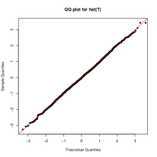
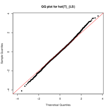
I will initially summarize results using QQ plots, based on 3,000 replications, comparing the simulated quantiles of and to quantiles of their baseline.
The resulting QQ plots for and are given in the left hand side of Figure 2 for . The results for are strong, matching the Gaussian limit theorem throughout except perhaps in the very extreme tails. The results for are terrible.
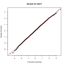
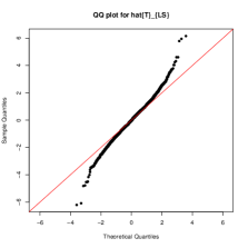
Perhaps poor behavior for is to be expected given is low.
The right hand side of Figure 2 gives the results for the corresponding easier case of . The performance of does not change very much, again providing very solid results. The is much better than in the heavier tail case, no longer terrible, just poor. This case is a situation where the limit theory for is valid, it is just not very accurate in practice.
5.2 More extensive experiments
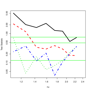
To compare performance in a wide set of diverse environments, I used the Cramér-von-Mises statistic to measure how non-Gaussian replications of and were, for a variety of values of and , as well as . The Cramér-von-Mises test statistic is reviewed in Baringhouse and Henze (2017). It is viewed as one of the most powerful distributional tests. To benchmark the values of the Cramér-von-Mises statistic of normality, the green horizontal lines are the 0.5, 0.95 and 0.99 quantiles of the distribution of the Cramér-von-Mises test statistic computed using 500,000 replications under the null of i.i.d. . The test is implemented in R using the function cvm.test(data, "pnorm",mean=0,sd=1).
The results are given in Figure 3. Crucially, notice that all plots use log-scales on both the -axis and the -axis. The dotted red line is the result for , while the black line is the corresponding results for . The -axis is the value of ; the -axis is the Cramér-von-Mises test statistic. The 1st and 3rd graph have , the 2nd and 4th have . The left hand side corresponds to , the right hand side .
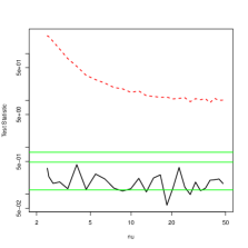
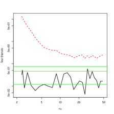
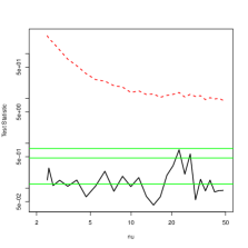
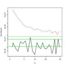
The results for are encouraging. Even with 500,000 replications it is typically not possible to reasonably reject normality of even with . When is at the bottom end of the plots, and , there is some evidence of a tiny amount of non-normality. The value of does not impact the results materially. As increases to 250 the results improve, a little.
For the results uniformly reject normality, typically dramatically. As increases the rejections become less significant, as expected. As increases to 250 the results improve, but only by a little.
5.3 Pushing to the case where
To assess the approximation for when , I ran a separate experiment. This experiment is less relevant to major equity data, although some commodity market price moves have extraordinarily thick tails and it is interesting theoretically. I excluded from consideration, as the previous experiment has shown it would have weak performance and the asymptotics is far from being valid.
It was less than clear to me how to generate predictors which are broadly comparable in scale across difference values of . I eventually settled on
which scales the student-t random variable so whatever the value of .
Figure 4 shows the results for (black line), (red dotted line), (green dots) and (blue line), here with throughout. The Figures again plot the Cramér-von-Mises test statistic against based on replications.
The results are encouraging, although not entirely positive. For small and small , significant distortion is present. Samples of around 1,000 do deliver results for which are hard to reject from a null of , even in cases where the predictors are just slightly less thick tailed than Cauchy.
Without the weighting function in , these simulations fall apart when . In that situation, I found no sign that increasing improves the behavior of . This is in line with the suggestions from the theory than once moments somewhat above the second do to not exist then the weight function becomes useful and eventually essential if . I recommend always including the weight function in practice. It is harmless for thin tailed data and essential for very thick tailed data.
6 Empirical work
6.1 Background
Some investors, such as young workers saving into pensions who do not have a mortgage, are unable to take on the level of financial leverage they may rationally desire due to administrative rules or the inability to borrow against their human capital. One viable investment strategy is to overweight their portfolio with high beta stocks, that is, stocks which move more strongly with the main market indexes than most stocks. This is discussed in Black (1972), amongst others. In finance betas are usually measured by regressing the returns on the individual stock on a wide market index. Such betas are used directly in vast numbers of empirical papers and drive other methods such as “Fama-MacBeth regressions”. All of these empirical results are fragile due to the thick tailed index returns.
Typically high beta investments will have high risk in order to potentially capture high expected returns. The opposite of this is attractive to a different type of investor. Some investors search out low beta stocks, hoping to have low risk, positive risk premium although relatively low expected return. This is discussed in Baker et al. (2011), who also review the extensive literature on this topic.
6.2 Selection by hypothesis test
But how to select high beta stocks and low beta stocks? Once selected, these groups of stocks could potentially be placed into portfolios or packaged as low and high beta ETFs.
In this Section selection will be regarded as a hypothesis testing problem. The -th stock will be labelled a high beta stock if we can reject the null
where is the beta of the -th stock.
I will label the -th stock a low beta stock if the null
is rejected.
The tests will be based on the approximate pivots
rejecting the nulls using a one-sided test with nominal size of 5%. I will compare the results for with the one based on .
6.3 Data
I downloaded the data from Yahoo for stock prices from 1 August 2018 to 4th August 2020. The S&P500 was measured using the SPDR S&P 500 ETF Trust (SPY). I converted these into weekly percentage arithmetic returns. These weekly returns will be compared to the returns on 416 individual stocks, which are components of the S&P500. The list of the stocks is available in RegFinance1.r, which produces all the results given in this Section.
Why weekly returns? There are virtues in using higher frequency data than weekly returns to estimate betas. In theory they can produce vastly more precise estimates. High frequency versions of regression include Barndorff-Nielsen and Shephard (2004), Barndorff-Nielsen et al. (2011) and Bollerslev et al. (2020). These sophisticated data hungry methods try to overcome the impact of nonsynchronous trading and differential rates of price discovery. However, they miss the impact of overnight returns. Daily returns capture overnight effects, but have significant lead-lag correlations. The hope with weekly returns is that most of the impact of these dependencies will be averaged away or dwarfed by other long-term effects. Many practitioners go further than this and use 2 to 5 years of monthly returns, but we do not follow that route. Further, some of the volatility clustering seen in finance is taken out by using weekly returns rather than high frequency returns.
6.4 Cross-sectional results
The right hand side of Figure 5 plots the cross-section of against . The left hand side gives the corresponding result for . The major impact of moving from to is that delivers some estimators with tiny standard errors, which is not the case with .

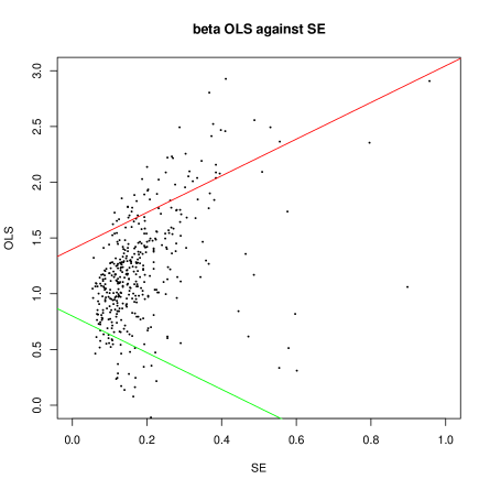
Indeed the smallest standard error for in the cross-section is around 0.054, while the minimum for is around 0.080 — around 50% higher.
Table 1 provides summary statistics on the cross-section of and . The estimates have roughly the same level, with roughly the same spread. The are slightly lower than the in this sample, across the distribution. Over the entire cross-section is a little above , as we would expect, but the difference is very modest. This suggests that a potential worry over being generally much less precise than is not compelling here. Table 1 also details the cross-section of against . These are very similar, which is also true of the and .
| Mean | 1.17 | 1.21 | 0.184 | 0.184 | 0.067 | 0.100 | 0.402 | 0.420 |
|---|---|---|---|---|---|---|---|---|
| Q(0.1) | 0.619 | 0.644 | 0.103 | 0.087 | -0.548 | -0.427 | 0.240 | 0.247 |
| Q(0.5) | 1.16 | 1.17 | 0.155 | 0.152 | 0.164 | 0.148 | 0.347 | 0.359 |
| Q(0.9) | 1.76 | 1.83 | 0.287 | 0.304 | 0.546 | 0.547 | 0.603 | 0.663 |
The left hand side of Figure 6 plots against in the cross-section. The blue line is a 45 degree line, while a cross-sectional regression of against yields an intercept of 0.150 (S.E. of 0.026) and slope of 0.849. The . The least squares linear regression line is shown in the figure by the red line. Overall the picture shows the two sets of estimates are comparable. The tend to be slightly pulled up for low betas and pulled down for high betas, when lined up with the corresponding .
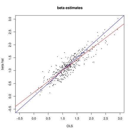
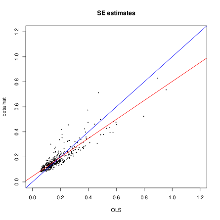
The right hand side of Figure 6 plots against in the cross-section. The blue line is a 45 degree line, while a cross-sectional regression of against yields an intercept of 0.045 (S.E. of 0.004) and slope of 0.757. The . The least squares linear regression line is shown in the Figure by the red line. When the S.E.s are low the is materially higher than the . However, for high S.E.s this is not the case. There is more discordance between and than and . In terms of against , they have a correlation of about 0.94, so are not plotted here.
Overall, these summary measures suggest that inference based on and may yield less extreme conclusions than those based on and .
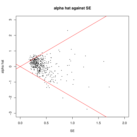
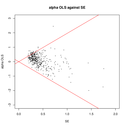
Figure 7 mimics Figure 5, but now for alpha. The differences between , and , are much smaller than in the beta case. Inference based on and should be very similar to that based on and .
Figure 5 shows the critical values for and for the high beta null, plotted as the red line (with an intercept of 1.4 and slope of 1.64). Any estimate above the red line corresponds to a statistically significant high beta. The corresponding results below the green line are statistically significant low beta stocks.
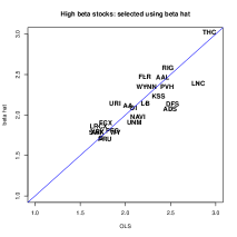
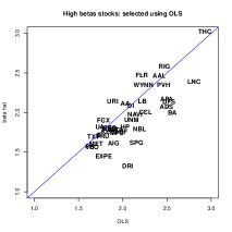
Table 2 provides a summary of the results from the tests for the nulls for the high and low betas. For both tests, it gives the number of rejections of the null together with the number of agreements. For the high beta stocks tests are much more liberal than . It is rare for to find a high beta stock which is not found by , but common to see high beta stocks selected by but not . The results are more scattered for the test of the low beta stocks.
| Agree | |||
|---|---|---|---|
| High beta | 36 | 49 | 32 |
| Low beta | 37 | 32 | 23 |
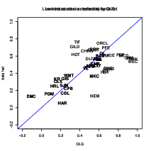
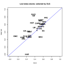
This is highlighted by Figure 8, plotting against for selected stocks. The 1st and 3rd selection is carried out by , the 2nd and 4th by . The left hand side of the Figure shows results for the selection of high beta stocks. The right hand side gives the corresponding selected low beta stocks. The labels are the individual stock tickers.
For the high beta selections, the selected stocks have both estimators and indicating pretty high betas. When the selection is based on the results are more variable.
For low beta selection, the story is much more mixed.
6.5 Rolling betas
Empirical researchers often deal with time-varying betas by using moving block, or rolling, averages — see Engle (2016) for an alternative model based approach and a discussion of the literature. In our context a rolling average approach computes the statistics and on the last 100, say, weeks of data, moving that window through time.
What do the pairs ,, and the two pair of pairs (corresponding to the high and low beta hypotheses) look like over the last 15 years for the first stock in our database, ABT, Abbott Laboratories? Now the data starts on 1 January 2005 and the rolling window always covers 100 weeks of data. In this entire database there are 358 stocks.
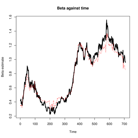

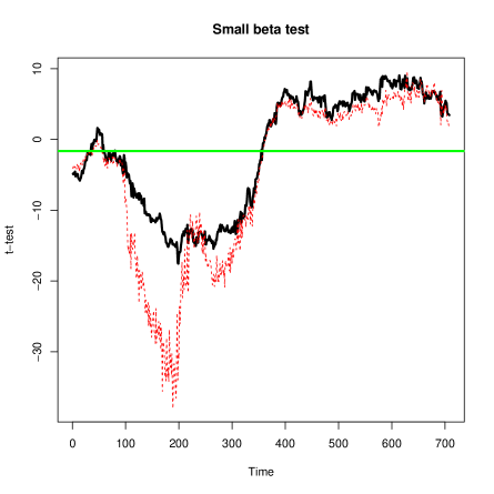
Figure 9 contains the results for ABT: is drawn using a thick black line; using a dotted red line. The beta estimates , broadly track one another. The coefficient does not go as high as the during higher beta periods, nor as low during lower beta periods.
I would like you to mostly focus on is the right hand side picture, which plots the pair through time. Although they follow the same general level through time, is very rough, sometimes moving dramatically over a few datapoints, as individual pairs of data fall in or out of the 100 day window. This is exactly what was feared in the introduction, it is very sensitive to large moves in the predictors. is much smoother, as if it has been time-series smoother — but it has not been. It drifts down and then up, the range moving by a factor of 2 in the picture.
This result is typical in the cross-section. Averaging over all time periods and across all stocks, the first element of Table 3 shows the square root of the average squared 100 times the daily time series changes in . This is just below 2.5, while the corresponding result for is around 15% higher. There are much bigger differences in the roughness of the standard deviations. The average movement of is around 70% higher than the result for .
| 2.44 | 2.84 | 0.152 | 0.269 |
|---|
One implication of this can be seen in Figure 10 for ABT. On the left hand side the pair is plotted against time for the large beta hypothesis test. The test based on least squares is very jagged through time, moving around week by week dramatically. The main driver of these moves are the jagged standard errors. The thick black line, corresponding to is again smooth. The same holds for the small beta test picture, which is the right hand side picture. Here the test rejects the null and selects this stock as a small beta stock for roughly the same period, but this is lucky for the evidence is very strong which makes choosing between using and moot.
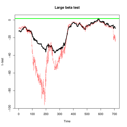
The evidence from looking at rolling betas is that the classic standard errors move around dramatically, easily upended by a single pair of data. More solid inference can be carried out using .
6.6 Rolling low and high beta portfolios
Using hypothesis tests based on the rolling estimates ,, and corresponding standard errors , I built each week an equal weighted high beta and low beta portfolio. The stocks are selected using a hypothesis test, which means the number of stocks in portfolio is random — an alternative would be to put a fixed number of stocks in the portfolio, selecting the stocks with the lowest -values. These portfolios are then used through the next week’s data to form a return over a week. This procedure is run through the entire sample period. Table 4 reports out of sample summary statistics of these two portfolios.
The results for the portfolio selected using test statistics based on and are similar.
The high beta portfolios produce what is expected: a higher average return and a substantially higher standard deviation, compared to the index. Their Sharpe ratios are not very different than the index, while their own betas are high, around 1.75, while the corresponding alphas are statistically close to 0.
The statistic “Share” is the time series average of the proportion of the cross-section which is in the portfolio. Hence the low beta portfolio contains around 13% of the stocks, the high beta portfolios contain around 7%. The “” is the time series average of the difference in holdings, so if the universe of stocks is 1,000 and the “” then on average 1 stock moves into or out of the portfolio each week. In our case the universe of stocks is 358, so on average 3 stocks come into or out of the portfolios each week.
| Portfolio type | E | sd | Sharpe | alpha | beta | Share | |
|---|---|---|---|---|---|---|---|
| Index | 0.194 | 2.49 | 0.077 | 0 | 1 | 0 | 0 |
| Low beta | 0.213 | 1.96 | 0.109 | 0.093 (0.041) | 0.625 | 0.136 | 0.008 |
| Low beta | 0.222 | 1.88 | 0.118 | 0.111 (0.042) | 0.573 | 0.137 | 0.008 |
| High beta | 0.361 | 5.05 | 0.071 | 0.018 | 1.77 | 0.076 | 0.007 |
| High beta | 0.359 | 5.09 | 0.070 | 0.018 | 1.75 | 0.076 | 0.006 |
The low beta portfolios are more interesting economically: their low beta should deliver a portfolio with low average returns and low standard deviations, but actually the average returns are higher than for the index, and this pushes the Sharpe ratio up. When these portfolios are regressed against the index, the betas are around two thirds, while they have positive alpha (the figure in brackets are standard errors). This is certainly not an unexpected result from the applied finance literature. The low beta premium is reported extensively in the literature, see Baker et al. (2011) for a review.
7 Median predictive regression
To finish the substance of this paper, it is useful to note that some of these points generalize.
Write denotes the -th quantile of the generic scalar random variable . The classic text on quantile regression is Koenker (2005). Here the focus will be on the “median predictive regression,” the case where , but the ideas hold for general quantile predictive regressions. To match the above treatment of linear predictive regression, the focus will be on the centered parameterization
| (7) |
is the estimand and inference about is my goal.
Inference on is traditionally based on the storied least absolute deviation estimator
whose asymptotic variance is typically estimated by
where and the shrinking bandwidth and as increases. This approach needs at least four moments (e.g. assuming the density of is bounded) of the predictors to yield asymptotically valid inference. Hence LAD based inference is, in my opinion, also not credible for financial economics. It has the same problem as inference for least squares under heteroskedasticity. This lack of credibility also directly applies, in my opinion, to the celebrated Koenker and Bassett (1978) check based estimator for quantile regression (recall it is the LAD estimator in the 0.5-quantile case).
For median predictive regression I advocate
noting is convex in , the and has subderivative
As before so . Hence is robust, having a bounded loss function and a bounded subderivative (Mallows (1975a, b), Krasker and Welsch (1982) and Giloni et al. (2006))111The approach can be made even more robust by reparameterization the predictive median regression, replacing the center by the element-by-element median, then taking as the element-by-element sample median allowing . This then contributes to , where I have normalized by , avoiding any squaring of data. Then has the same characteristics as before. . Inference will be based on
where and the shrinking bandwidth and as increases.
is applied to the preprocessed data and . The preprocessing stabilizes statistical inference, while existing software can be used without any further changes to find .
Example 6
If there is no intercept and a single predictor, then and
so implying
the median slope from to . This has some similarities to the Theil–Sen estimator and the repeated median estimator.
Feasible inference for will be valid if the predictors have at least two moments. Hence these assumptions are plausible for data in financial economics. To formalize this, the Assumptions will again be written in two blocks.
Assumption 3
-
C1.
Assume , write and define
-
C2.
There exists a single such that
so all .
-
C2.
is a continuous random variable with a conditional density .
-
D1.
are i.i.d.;
-
D2.
;
-
D3.
is positive definite.
Theorem 6 provides the main features of .
Theorem 6
is convex in and
Under Assumptions C1-C3 and D1-D3, as increases
further
where, writing ,
Proof: Given in the Appendix.
To carry out inference and need to be estimated well. I advocate and : this is discussed in Section 9.5 in the Appendix.
8 Conclusions
I have advocated estimating linear in parameters predictive regressions using rather than the celebrated least squares estimators . Why? has relatively simple standard errors which are robust to thick tailed predictors. This robustness leads, in practice, to nominal tests which are close to being valid (i.e. correct size), as well as standard errors which a reasonable smooth through time for rolling estimators.
There are downsides with . gains precise from being super sensitive to unusual predictors. downweights these low probability but influential predictors. Sometimes it is good to take full advantage of every scrap of available information. In that case it makes sense to use . But replication and testing in that environment will be fragile, sensitive to one or two datapoints. is a more conservative estimator, it even works with data as thick tailed as nearly Cauchy. Empirically in finance, the average standard deviation for is close to , so the practical loss of precision seems modest.
The concerns and solutions extend to quantile regression. Inference base on is not robust to thick tailed predictors, while is. It raises no new issues in terms of computation.
9 Appendix
9.1 Proof of Theorem 3
Now
and
Now
so that
Rearranging gives the result for . Note that
Then
then using a matrix inverse gives the result.
9.2 Proof of Theorem 4
B1 is needed for to exist. Define the predictive regression errors , for . Then
Then under A2 and B2,
while under B2 and B3
Then the conditional unbiasedness and conditional variance follow.
What remains is the Berry-Esseen type result. The approach is to use the Bentkus (2005) version. It is stated here for convenience.
Theorem 7
(Bentkus (2005)) Suppose are zero mean, independent in , then
where
where denotes the set of all convex subsets of
Now
The are conditionally independent with variances
and the corresponding sums
is invertible using B1 and B4. Then
which is positive definite, so
Then define the corresponding skewness terms
which exists using B5.
9.3 Proof of Theorem 5
Stack the moment conditions:
where . Crucially does not depend upon . Then
while
where here I write and . Of course
The crucial matrix zeros follow by Adam’s law applied to
Further,
The term is not of central importance, but takes the form
Finally, notice A3 means that is symmetric and invertible. The result then follows conventionally.
QED.
9.4 Proof of Theorem 6
We start with a statement and proof of a preliminary theory.
Theorem 8
, then is convex in , writing , then
and
and under C2
Under C1 and C2, define and . Then
Proof.
Ignore subscripts
so is convex. Scaling by has no impact on convexity.
Define and , then
and so by triangular inequality
By Cauchy-Schwartz
Applying the same argument the other way, we have
so
This bounding implies all moments of must exist.
The subderivative is straightforward, as is the stated conditional variance as
and the squared sign function is . Now let , then
Now, for ,
and, for ,
Hence
using the convention . Then so assuming range of does not depend upon , using Leibnitz’s rule
The results on the moments of are straightforward.
QED.
We now move to the proof of the main parts of the theorem.
Proof of Theorem 8, shows that
so the mean of exists. Theorem 8 says is convex and thus so is , as indeed is . Under D1, the strong law of large numbers (10) implies
| (10) |
As is convex, pointwise convergence implies uniform convergence.
All that remains is to check that is the global minimizer of the convex ? We know this from the derivative and second derivative of with respect to evaluated at so long as exists. But Assumption Q4 is enough to guarantee this. D3 is enough for this to to be guaranteed to be a unique minimum at .
Now turn to the CLT.
Recall under C1 and D2, exists. Further, under C1,C2 and D2 exists. Additionally under D3, it is also positive definite. The sole challenge here is that is not differentiable at for which and has derivatives which are either 0 or not defined.
We use a stochastic equicontinuity argument. A review is provided by Andrews (1994). Now write
which is the sums of i.i.d. terms, while recall is bounded above by 1. Further, in the special case , and .
By mean value Theorem, there exists a such that
Now so
Hence
The challange is the limit law of
As is always bounded above and below by 1, this setup is contained in type I class of Andrews (1994), so the law of is the same as the law of . But that law follows from Lindeberg-Levy CLT
The rest is straightforward.
QED.
9.5 Estimating the asymptotic variance
Focus on the two stage method of moment estimator. Now
by, respectively, the strong law of large numbers and the uniform strong law of large numbers as for all . So
The harder term is and, for a bandwidth , the
Suppose we had some data then estimate the joint density by the kernel
where are zero mean kernel densities, and plug it into
This suggests the use a rectangular kernel
which needs and as increases so long as
Here .
References
- Andrews (1994) Andrews, D. W. K. (1994). Empirical process methods in econometrics. In R. F. Engle and D. McFadden (Eds.), Hanbook of Econometrics, Volume 4, pp. 2247–2294. Elsevier.
- Andrews et al. (2019) Andrews, I., J. Stock, and L. Sun (2019). Weak instruments in IV regression: Theory and practice. Annual Review of Economics 11, 727–753.
- Baker et al. (2011) Baker, M., B. Bradley, and J. Wurgler (2011). Benchmarks as limits to arbitrage: Understanding the low‐volatility anomaly. Financial Analysts Journal 67, 1–15.
- Balkema and Embrechts (2018) Balkema, G. and P. Embrechts (2018). Linear regression for heavy tails. Risks 6, 1–70.
- Baringhouse and Henze (2017) Baringhouse, L. and N. Henze (2017). Cramér–von Mises distance: probabilistic interpretation, confidence intervals, and neighbourhood-of-model validation. Journal of Nonparametric Statistics 29, 167–188.
- Barndorff-Nielsen et al. (2011) Barndorff-Nielsen, O. E., P. R. Hansen, A. Lunde, and N. Shephard (2011). Multivariate realised kernels: consistent positive semi-definite estimators of the covariation of equity prices with noise and non-synchronous trading. Journal of Econometrics 162, 149–169.
- Barndorff-Nielsen and Shephard (2004) Barndorff-Nielsen, O. E. and N. Shephard (2004). Econometric analysis of realised covariation: high frequency covariance, regression and correlation in financial economics. Econometrica 72, 885–925.
- Bentkus (2005) Bentkus, V. (2005). A Lyapunov-type bound in . Theory of Probability and its Applications 49, 311–323.
- Black (1972) Black, F. (1972). Capital market equilibrium with restricted borrowing. Journal of Business 4, 444–455.
- Blattberg and Sargent (1971) Blattberg, R. and T. J. Sargent (1971). Regression with non-Gaussian disturbances: Some sampling results. Econometrica 39, 501–510.
- Bollerslev et al. (2020) Bollerslev, T., A. Patton, J. Li, and R. Quaedvlieg (2020). Realized semicovariances. Econometrica. Forthcoming.
- Butler et al. (1990) Butler, R. J., J. B. MacDonald, R. D. Nelson, and S. B. White (1990). Robust and partially adaptive estimation of regression models. The Review of Economics and Statistics 72, 321–327.
- Cauchy (1836) Cauchy, A. (1836). On a new formula for solving the problem of interpolation in a manner applicable to physical investigations. Philosophical Magazine 8, 459–468.
- Cont (2001) Cont, R. (2001). Empirical properties of asset returns: Stylized facts and statistical issues. Quantitative Finance 1, 223–236.
- Eicker (1967) Eicker, F. (1967). Limit theorems for regressions with unequal and dependent errors. In Proceedings of the Fifth Berkeley Symposium on Mathematical Statistics and Probability, Volume 1, pp. 59–82. Berkeley: University of California.
- Engle (2016) Engle, R. F. (2016). Dynamic conditional beta. Journal of Financial Econometrics 14, 643–667.
- Farebrother (1999) Farebrother, R. W. (1999). Fitting Linear Relationships: A history of the calculus of observations 1750–1900. New York: Springer.
- Giloni et al. (2006) Giloni, A., J. Simonoff, and B. Sengupta (2006). Robust weighted LAD regression. Computational Statistics and Data Analysis 50, 3124–3140.
- Gorji and Aminghafari (2019) Gorji, F. and M. Aminghafari (2019). Robust nonparametric regression for heavy-tailed data. Journal of Agricultural, Biological, and Environmental Statistics. Forthcoming.
- Hall (1992) Hall, P. G. (1992). The Bootstrap and Edgeworth Expansion. New York: Springer.
- Hallin et al. (2010) Hallin, M., Y. Swan, T. Verdebout, and D. Veredas (2010). One-step R-estimation in linear models with stable errors. Journal of Econometrics 172, 195–204.
- Hampel et al. (2005) Hampel, F., E. M. Ronchetti, P. J. Rousseeuw, and W. A. Stahel (2005). Robust Statistics: The Approach based on Influence Functions. New York: Wiley.
- Hausman and Palmer (2012) Hausman, J. and C. Palmer (2012). Heteroskedasticity-robust inference in finite samples. Economics Letters 116, 232–235.
- Heyde and Seneta (1977) Heyde, C. C. and E. Seneta (1977). I.J. Bienayme. Statistical Theory Anticipated. Springer. Studies in the History of Mathematics and Physical Sciences, volume 3.
- Hill and Renault (2010) Hill, J. B. and E. Renault (2010). Generalized method of moments with tail trimming. Unpublished paper: Department of Economics, UNC.
- Huber (1967) Huber, P. J. (1967). The behavior of maximum likelihood estimates under nonstandard conditions. In Proceedings of the Fifth Berkeley Symposium on Mathematical Statistics and Probability, pp. 221–233. University of California Press.
- Ibragimov et al. (2020) Ibragimov, R., J. Kim, and A. Shrobotov (2020). New robust inference for predictive regressions. Unpublished paper: Imperial College, London.
- Kim and Meddahi (2020) Kim, J. and N. Meddahi (2020). Volatility regressions with fat tails. Journal of Econometrics. Forthcoming.
- King and Roberts (2015) King, G. and M. E. Roberts (2015). How robust standard errors expose methodological problems they do not fix, and what to do about it. Political Analysis 23, 159–179.
- Koenker (2005) Koenker, R. (2005). Quantile Regression. Cambridge: Cambridge University Press.
- Koenker and Bassett (1978) Koenker, R. and G. Bassett (1978). Regression quantiles. Econometrica 46, 33–50.
- Krasker and Welsch (1982) Krasker, W. S. and R. E. Welsch (1982). Efficient bounded-influence regression estimation. Journal of the American Statistical Association 77, 595–604.
- Kurz-Kim and Loretan (2014) Kurz-Kim, J. and M. Loretan (2014). A note on the coefficient of determination in regression models with infinite-variance variables. Journal of Econometrics 181, 15–24.
- Linnik (1961) Linnik, Y. (1961). Method of Least Squares and Principal Theory of Observations. New York: Pergamon Press.
- MacKinnon and White (1985) MacKinnon, J. G. and H. White (1985). Some heteroskedastic-consistent covariance matrix estimators with improved finite sample properties. Journal of Econometrics 29, 305–325.
- MacKinnon (2012) MacKinnon, R. (2012). Thirty years of heteroskedasticity-robust inference. In X. Chen and N. Swanson (Eds.), Recent Advances and Future Directions in Causality, Prediction, and Specification Analysis, pp. 437–461. Springer.
- Mallows (1975a) Mallows, C. L. (1975a). Influence functions. Presented at the NBER conference on Robust Regression, Cambridge, MA.
- Mallows (1975b) Mallows, C. L. (1975b). On some topics in robustness. Unpublished paper: Bell Telephone Laboratories, Murray Hill, New Jersey.
- Mikosch and de Vries (2013) Mikosch, T. and C. G. de Vries (2013). Heavy tails of OLS. Journal of Econometrics 172, 205–21.
- Newey and McFadden (1994) Newey, W. K. and D. McFadden (1994). Large sample estimation and hypothesis testing. In R. F. Engle and D. McFadden (Eds.), The Handbook of Econometrics, Volume 4, pp. 2111–2245. North-Holland.
- Nolan and Ojeda-Revah (2013) Nolan, J. P. and D. Ojeda-Revah (2013). Linear and nonlinear regression with stable errors. Journal of Econometrics 172, 186–194.
- Phillips et al. (2004) Phillips, P. C. B., J. Y. Park, and Y. Chang (2004). Nonlinear instrumental variable estimation of an autoregression. Journal of Econometrics 118, 219–246.
- Samorodnitsky et al. (2007) Samorodnitsky, G., S. T. Rachev, J.-R. Kurz-Kim, and S. V. Stoyanov (2007). Asymptotic distribution of unbiased linear estimators in the presence of heavy-tailed stochastic regressors and residuals. Probability and Mathematical Statistics 27, 275–302.
- Seal (1967) Seal, H. L. (1967). Studies in the history of probability and statistics. XV: The historical development of the Gauss linear model. Biometrika 67, 1–24.
- So and Shin (1999) So, B. S. and D. W. Shin (1999). Cauchy estimators for autoregressive processes with applications to unit root tests and confidence intervals. Econometric Theory 15, 165–176.
- Sun et al. (2020) Sun, Q., W. Zhou, and J. Fan (2020). Adaptive Huber regression. Journal of the American Statistical Association 115, 254–265.
- White (1980) White, H. (1980). A heteroskedasticity-consistent covariance matrix estimator and a direct test for heteroskedasticity. Econometrica 48, 817–838.