Gravity field modeling using space frequency signal transfer technique between satellites
Abstract
Here we provide an alternative approach to determine the Earth’s external gravitational potential field based on low-orbit target satellite (TS), geostationary satellites (GS), and microwave signal links between them. By emitting and receiving frequency signals controlled by precise clocks between TS and GS, we can determine the gravitational potential (GP) at the TS orbit. We set the TS with polar orbits, altitude of around 500 km above ground, and three evenly distributed GSs with equatorial orbits, altitudes of around 35000 km from the Earth’s center. In this case, at any time the TS can be observed via frequency signal links by at least one GS. In this way we may determine a potential distribution over the TS-defined sphere (TDS), which is a sphere that best fits the TS’ orbits. Then, based on the potential distribution over the TDS, an Earth’s external gravitational field can be determined. Simulation results show that the accuracy of the potential filed established based on 30-days observations can achieve decimeter level if optical atomic clocks with instability of are available. The formulation proposed in this study may enrich the approachs for determining the Earth’s external gravity field.
JGR: Solid Earth
School of Resource, Environmental Science and Engineering, Hubei University of Science and Technology, Xianning, Hubei, China Time and Frequency Geodesy Research Center, Department of Geophysics, School of Geodesy and Geomatics, Wuhan University Key Lab of Surveying Eng. and Remote Sensing, Wuhan University
WenBin Shenwbshen@sgg.whu.edu.cn \correspondingauthorXinyu Xuxyxu@sgg.whu.edu.cn
Low- and high-orbit satellites are connected by frequency links controlled by precise clocks.
Gravitational potential along the orbit of low-orbit satellite is determined.
Optic-clock-based Earth’s gravity field could be established.
1 Introduction
The Earth’s gravity field is a fundamental physical field of the Earth. Since gravity field has various and significant applications in many fields and branches, its determination is one of the main tasks in geodetic community. If the density distribution of the Earth is given, one may determine the gravitational potential (GP) field both inside and outside the Earth (namely in whole space domaion) by Newtonian integral formula, and consequently the gravity field in whole space is determined by applying the gradient operator to the gravity potential (geopotential) field, where geopotential is the sum of GP and the centrifugal force potential generated by the Earth’s rotation. However, since the Earth’s density distribution (e.g. the preliminary reference Earth model, PREM) (Dziewonski \BBA Anderson, \APACyear1981) was poorly determined, the gravity field determined based on density distribution cannot satisfy the general application requirements. Fortunately, one can determine the external gravity field with successive accuracy requirement if some kind of distribution related to gravity (for instance the gravity distribution or gravity potential distribution) over the Earth’s surface (boundary) is given (Hofmann-Wellenhof \BBA Moritz, \APACyear2005). How to determine a gravity field (or equivalently gravity potential field) based on the given distribution values on the boundary (e.g. the Earth’s surface) is referred to as the geodetic boundary value problem (GBVP). A generally accepted approach to solve this boundary problem is to use the spherical harmonic analysis, which can successfully express the external gravity field once a full coverage of the gravity (or geopotential) measurements over the Earth’s surface or a surface (e.g. a surface defined by the orbits of a flying satellite) enclosing the whole solid Earth is provided. To overcome difficulties in practical measurements on the Earth’s surface, especially in mountain areas and ocean areas, there appeared different satellite-based gravity measurement techniques, which have their own advantages especially in the aspect of full coverage over the Earth.
Kaula (\APACyear1966) proposed the method of establishing gravity model by observing the orbit perturbation of artificial satellites, and solve the coefficient of GP. Since the new satellite gravity missions appeared (e.g., the CHAMP mission (Reigber \BOthers., \APACyear2002) launched on 2000, the GRACE twin satellite mission (Tapley \BOthers., \APACyear2004) launched on 2002, the GOCE mission launched on 2009), scholars have paid extensive attention on the recovery of satellite gravity field and various methods have been proposed, such as orbital perturbation (Hwang, \APACyear2001), harmonic analysis (Reubelt \BOthers., \APACyear2003), satellite accelerations (Ditmar \BBA Sluijs, \APACyear2004) and energy integral (Jekeli, \APACyear1999; Han \BOthers., \APACyear2002; Visser \BOthers., \APACyear2003). These satellite-based gravity measurement techniques have their own advantages especially in the aspect of full coverage over the Earth.
For example, the Gravity Field and Steady-State Ocean Circulation Explorer (GOCE) mission, which aims to make detailed measurements of Earth’s gravity field, leading to discoveries about gravity field determination and ocean circulation investigations (Drinkwater \BOthers., \APACyear2003; Hirt \BOthers., \APACyear2012). GOCE satellite system flies in a near-polar orbit with an altitude of about 250 km above the ground, consisting of an on-board three-axis gravity gradiometer, GNSS receiver, satellite-to-satellite tracking and relevant equipments (Bock \BOthers., \APACyear2011; Hirt \BOthers., \APACyear2012). Concerning the global gravity field determination aspect, the GOCE’s mission may map gravity field features with 1 to 2 cm accuracy for geoid undulations and about 1 mgal for gravity, down to scales of about 100 km, or spherical harmonic degree about 200 (Pail \BOthers., \APACyear2011; Hirt \BOthers., \APACyear2012). Since the GOCE satellite retired in 2013, the current satellite gravity mission on-going is the GRACE Follow-On (Kornfeld \BOthers., \APACyear2019), which is a twin satellite system with the height of about 500 km. These satellite-based gravity measurements have greatly improved our understanding of the Earth’s gravity field (Flechtner \BOthers., \APACyear2016; Kvas \BBA Mayer-Gürr, \APACyear2019; Pail \BOthers., \APACyear2019).
In recent years, thanks to the quick development of time and frequency science, the optical-atomic clocks (OACs) with stability and accuracy better than level in several hours have been developed in laboratory environment (Mehlstäubler \BOthers., \APACyear2018; McGrew \BOthers., \APACyear2018; Huang \BOthers., \APACyear2019; Oelker \BOthers., \APACyear2019). Especially, portable and on-board-satellite clocks with ultra-high stability will be available in the near future (Schiller \BOthers., \APACyear2012; Altschul \BOthers., \APACyear2014; Hannig \BOthers., \APACyear2019). This provides potential realization in the near future to determine the GP differences between a satellite and a ground station using precise atomic-clock-related frequency signal links based upon general relativity theory (GRT) (Einstein, \APACyear1915). Suppose a satellite sends frequency signals and two receivers on different ground stations receive the signals, then the geopotential difference between the two stations can be determined by observing the frequency shift (W. Shen \BOthers., \APACyear2011). However, how to practically and precisely extract the frequency shift signals caused by the geopotential difference between a ground station and a satellite is a challenging problem, due to the fact that Doppler effects, ionosphere and troposphere effects contaminate the observations seriously. In order to overcome these difficulties, recently a more precise formulation of the satellite frequency signal transfer (SFST) approach based on tri-frequency combination technique was established (Z. Shen \BOthers., \APACyear2016, \APACyear2017), which aims to determine the GP difference between a satellite and a ground station or between two satellites at an accuracy level of several centimeters if high-precise frequency signal links are established. To precisely compare the frequency signals, the relative stability of clocks should reach about in several hours (corresponding to about 1 cm in height) for the practical applications of SFST method in geodesy.
Based on the SFST technique, in this study we formulate an alternative approach to determine the Earth’s external gravity field, which is completely different from the conventional ones. The basic idea, which was put forward several years ago by our group (Z. Shen \BBA Shen, \APACyear2017) is that the GP along a low-orbit target satellite (TS) can be determined using frequency signal links between TS and geostationary satellites (GSs). In section 2 we briefly introduce the relativistic geodesy and SFST technique, by which the GP difference between the TS and GS could be determined. Then we formulate an approach to show how to determine a GP distribution over a TS-altitude defined sphere (TSS), which is bounded by the flights of the TS and defined as the sphere that can best fit the TS’s orbits. Given the GP distribution over the TSS, a global gravity field (or Earth’s gravity model) could be determined. In sections 3 and 4, we conducted simulation experiments, and results show that the proposed approach in this study is prospective. In section 5 we summarize the main results and discuss relevant potential issues.
2 Method
2.1 Gravity frequency shift
The GRT predicts that the frequency (or tick rate) of a clock is related to the geopotentials at the place where the clock is located. Specifically, suppose two clocks are located at different positions and where the geopotential values are and respectively, and accurate to , the frequencies and of the two clocks satisfy the following equation (Weinberg, \APACyear1972; Bjerhammar, \APACyear1985)
| (1) |
where is the speed of light in vacuum, , are high order terms which can be neglected in the case that the two stations are in the vicinity of Earth. If the clock frequencies and are precisely measured and compared, the geopotential difference between and can be derived. The study of geodesy problems (such as geopotential determination) by the method of clock comparison is regarded as relativistic geodesy (Flury, \APACyear2016; Puetzfeld \BBA Lämmerzahl, \APACyear2019).
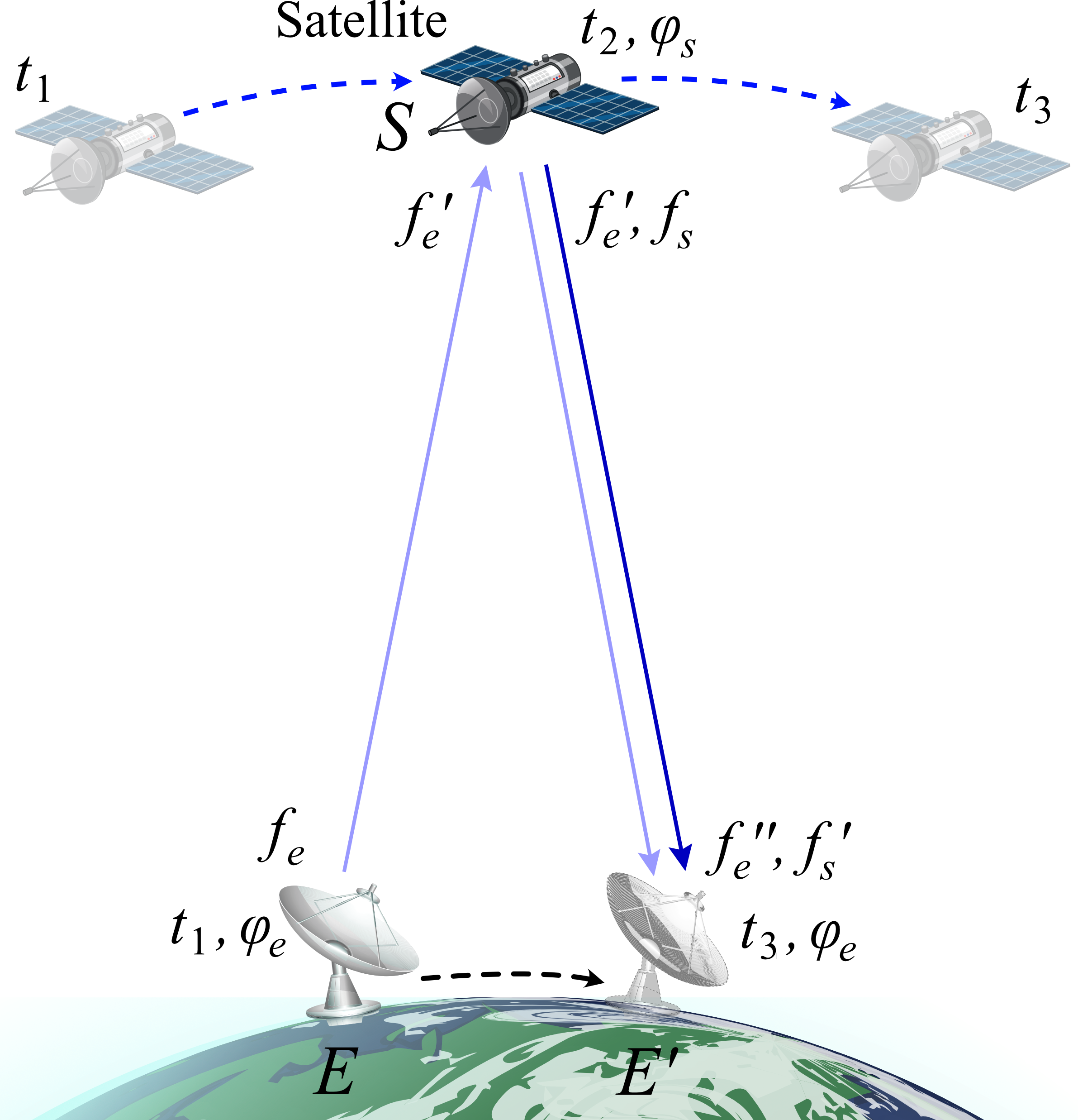
Currently, there are three kinds of method to compare clocks located at different places: (1) clock transportation (Kopeikin \BOthers., \APACyear2016; Grotti \BOthers., \APACyear2018), (2) transfer frequency signals via optical fibre links (Takano \BOthers., \APACyear2016; Wu \BOthers., \APACyear2019; Z. Shen, Shen, Peng\BCBL \BOthers., \APACyear2019), and (3) transfer frequency signals via satellite and free-space links (Deschênes \BOthers., \APACyear2016; Z. Shen \BOthers., \APACyear2017). The first two methods are suitable for clocks comparison on ground, while the third method is designed for satellite clocks comparison. But transferring frequency signals via satellite is much more complex than Eq. (1). For example, the satellite is in high-speed motion state which gives rise to Doppler effects; the mediums in space (such as ionosphere and troposphere) will also cause frequency shifts during a microwave or optical signal’s propagation through them. In order to address these problem, Kleppner \BOthers. (\APACyear1970) proposed a method to transfer microwave frequency signal between a satellite and a ground site; and it is successfully applied for verifying Einstein’s equivalence principle (Vessot \BBA Levine, \APACyear1979; Vessot \BOthers., \APACyear1980). The main idea of the frequency transfer method is that a satellite and a ground site are connected by 3 microwave links simultaneously (as depicted in Fig. 1). In this case the first order Doppler effect and most of the medium influence will be canceled out in the output beat frequency
| (2) |
where and are emitted frequency from ground site and satellite respectively; they are received as and at satellite and ground site respectively. For each microwave link, the emitted frequency values are different from the received values. When the frequency signal is received at satellite, it is transmitted immediately and received at ground site as . Details can be referred to Vessot \BBA Levine (\APACyear1979).
Kleppner’s method was later improved and introduced to relativistic geodesy for GP determination (Z. Shen \BOthers., \APACyear2016, \APACyear2017), and was regarded as satellite frequency signal transmission (SFST) method. According to SFST, the GP difference between a satellite and a ground site is given in the following form (Z. Shen \BOthers., \APACyear2017)
| (3) |
where is the GP difference between the satellite and the ground station, and are velocities of satellite and ground site respectively, () are quantities related to the positions and velocities of the satellite and ground site, second Newtonian potential, vector potential, and third- and forth-order terms, is the correction terms for ionospheric, tropospheric and tidal effect, denote high order terms that can be neglected. Details can be referred to Z. Shen \BOthers. (\APACyear2017).
The theoretical precision of Eq. (3) is at the level, much better than the original formula applied in GP-A experiment where its theoretical precision is limited to . The precision of SFST method for determining GP is about several centimeters, provided that the stability of OACs can reach level (Z. Shen \BOthers., \APACyear2017).
2.2 Determination of gravitational potential along the target satellite orbit
Suppose the GP value of a ground station is given, then we can determine the GP values of a satellite by establishing SFST links between them. If the GP distribution (GPD) over a TSS (e.g. GOCE-type or GRACE-type satellite) is determined, the Earth’s external gravity field can be determined correspondingly (see Sect. 4). However, since the orbit of a satellite for the purpose of determining the gravity field is relatively close to ground (e.g., the height of GRACE satellite is about 500 km), only a short arc length of the orbit is visible to a certain ground station. If we want to determine the GPD over the TDS, hundreds of ground datum stations with given GP values are needed in order to guarantee that the satellite can connect to at least 1 ground station at any time (Z. Shen \BOthers., \APACyear2018), which is impractical for the foreseeable future.
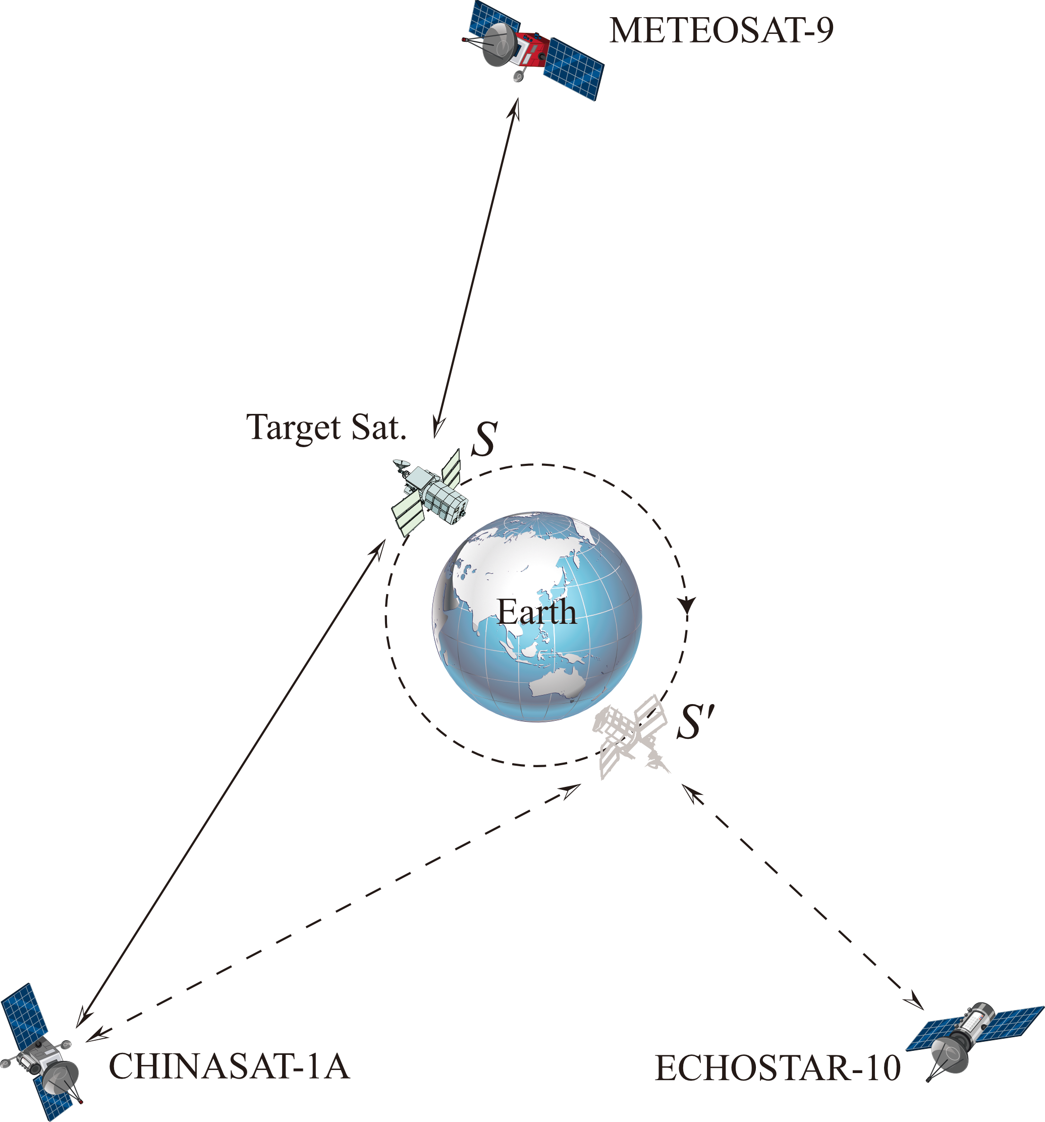
Although the SFST method described in Sect. 2.1 was originally designed for determining the GP difference between a satellite and a ground site, it can also be used for determining the GP difference between two satellites after some modification (Z. Shen, Shen\BCBL \BBA Zhang, \APACyear2019). Suppose a TS (with low earth orbit) is connected to a GS (with high earth orbit), then the setup of the SFST links between them are depicted as Fig. 2.
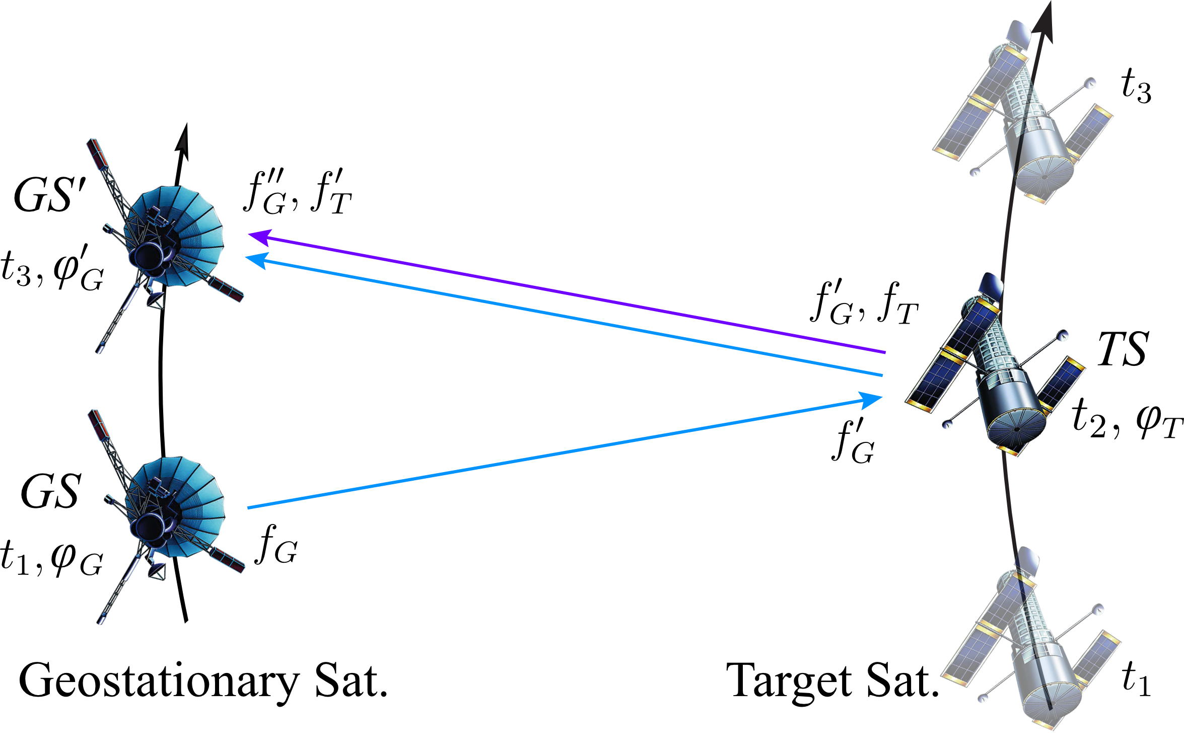
An emitter of the geostationary satellite emits a frequency signal at time . When the signal is received by the target satellite at time , it immediately transmits the received signal and emits a frequency signal simultaneously. These two signals transmitted and emitted from the satellite are received by a receiver at geostationary satellite at time , which are noted as and , respectively. During the period of the emitting and receiving, the position of the geostationary satellite in space has been changed from to . Since the target satellite transmits and emits signals at the same instant it receives signal; its position in the signal links is supposed to be the point at time . If we set , the gravitational difference between the and can be expressed as
| (4) |
where the foot mark and denote the and respectively, and the beat frequency is given by.
| (5) |
Note that there might be a small amount of latency during the transmitting, thereby the positions of the satellite is slightly different at the time it receives and emits signals. Suppose the delay of the signal transponder is about 800 ns (Pierno \BBA Varasi, \APACyear2013), and the orbit height of TS is about 500 km (the velocity is about 7.6 km/s); then the satellite moves only 0.62 mm between receiving and emitting signals, and this influence can be neglected for the SFST links (Z. Shen \BOthers., \APACyear2016).
Similar to the satellite-to-ground link, if the GP difference between the GS and TS are measured by SFST method, and the absolute GP values of the GS is given, then the GP values of the TS can be derived. The height of a GS is about 35790 km above the equator. If the TS is a low orbit satellite satellite whose height is about 500 km above the geoid (e.g., the case of GRACE-FO satellite), then the GS can cover more than half of the TS’s orbit sphere, as depicted in Fig. 3. Therefore only two evenly distributed GS is sufficient for incessantly SFST links between a GS and the TS, and the GP values of the TS’s orbit sphere can be determined correspondingly. However, in practice it is better to apply three evenly distributed GSs for more reliable and stable connections, as shown in Fig. 5
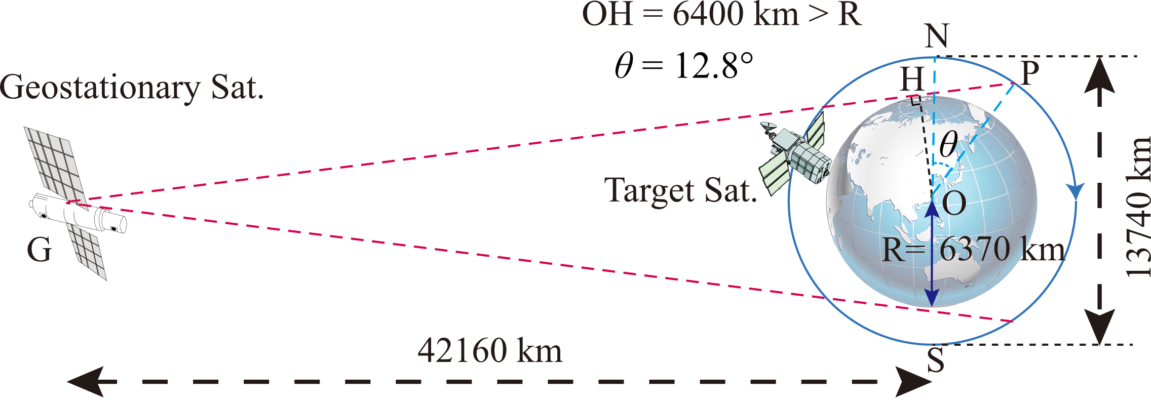
If the GPD over the TSS is given, one can derive the gravity field outside the TSS, and according to the spherical harmonic expansion formula, the determined gravity field outside the TSS can also be expanded to the Earth’s surface (Heiskanen \BBA Moritz, \APACyear1967).
3 Simulation Experiments
In this section we conducted several simulation experiments to verify the SFST method for satellite gravity model establishment. Currently, the most precise atomic clock onboard a satellite is only about ( in second) in stability (Laurent \BOthers., \APACyear2015; Liu \BOthers., \APACyear2018). While the best optical atomic clock on ground have reached the stability of (Oelker \BOthers., \APACyear2019). In the prospect of much better clocks onboard satellites in the future, our experiments will adopt different clock stability levels from to ; and the results can show us the minimum requirements of clock stability for a satellite gravity model in a certain precision.
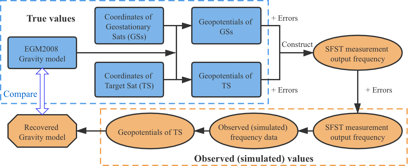
The scheme of a simulation experiment is comparing a prior satellite gravity model to a recovered one, as depicted in Fig. 4; details are explained in the following subsections.
3.1 Input data
In Sect. 2.2 we have shown that two GSs are sufficient for incessant SFST links to a TS. But in practice it is more reliable to adopt three evenly distributed GSs above the equator. Therefore in our experiments we chose the meteorological satellite METEOSAT-9 of EU (at 9.2∘E), the communication satellite CHINASAT-1A of China (at 130.0∘E), and the communication satellite ECHOSTAR-10 of US (at 110.2∘W) as the GSs; and the GRACE-FO 1 satellite (orbit height is about 500 km) as the TS. The setup of the experiment is depicted in Fig 5.
The orbital period of TS (GRACE-FO 1) is about 1.6 h, and the inclination of TS is about 89∘. For the purpose of obtaining the GP data over its orbit sphere with a resolution of , the observations should continue for at least 576 hours (24.0 day), with observation interval being smaller than 8.0 second. Therefore, we set the observational time span as 30.0 days, and the observation interval as 1 second, which fully satisfies the resolution requirements. For every observation the TS is connected to a nearest visible GS with SFST links. For the purpose of simulation, the orbits data of these four satellites (one TS and three GSs) can be generated from two-line element set (TLE) data by simplified general perturbations models 4 (SGP4) (Croitoru \BBA Oancea, \APACyear2016). The GPs at orbits of these satellites can be calculated by EGM2008 model (Pavlis \BOthers., \APACyear2012). Then the GP difference between the TS and one proper GS can be obtained. These data are all regarded as true values, hence the errors of orbit data and gravitational potential model EGM2008 are not considered.
The frequency of a microwave signal will be affected by ionosphere and troposphere environment. We adopt the International Reference Ionosphere Model (Rawer \BOthers., \APACyear1978; Bilitza \BOthers., \APACyear2017) to obtain the electron density values to estimate the ionospheric influence (Namazov \BOthers., \APACyear1975). Since the height of TS is about 500 km which is much higher than the troposphere layer (typically from ground to 60 km height), the influence of troposphere can be neglected. The GP at the satellites’ orbits will also be influenced by periodical tidal effects, which are well modeled (Voigt \BOthers., \APACyear2017) and can be removed by some mature softwares such as ETERNA (Wenzel, \APACyear1996) or Tsoft (Van Camp \BBA Vauterin, \APACyear2005). In our experiment we use ETERNA to generate and analyze tide signals. These tidal signals also include the influences of other planets (such as Venus, Jupiter etc.) besides the Sun and the Moon.
| Entities | Values of Parameters |
|---|---|
| GS Satellite | METEOSAT-9 |
| CHINASAT-1A | |
| ECHOSTAR-10 | |
| TS Satellite | GRACE FO 1 |
| Gravity field model | EGM2008 |
| Ionospheric model | International Reference Ionosphere |
| Tide correction | ETERNA |
| Observation duration | Jan 01 Jan 30, 2020 |
| Mearsurement interval | 1 s |
3.2 The “Observed” GP along the TS orbit
After setting the input data, the next step focuses on determining the GP values at TS’s orbit. There are 3 GSs, denoted as respectively. As we take a SFST measurement (every 1 second), we can obtain an observed GP difference value according to Eq. (4). If the GP of is given, the observed GP can be derived as .
The observed values are different from true GP value because they are influenced by various error sources. In this simulation experiment we have considered clock error , ionosphere residual error , satellite’s position and velocity errors and , GS’s potential errors and tidal correction residual error . The above mentioned various errors are considered as noises, which are added to the true values. The total errors are expressed in the following form
| (6) |
and the observed values can be expressed as
| (7) |
The magnitude and behavior of each kind of error play important role in this experiment; thereby we need to investigate different error models based on different error sources to make the simulation case more close to the real case.
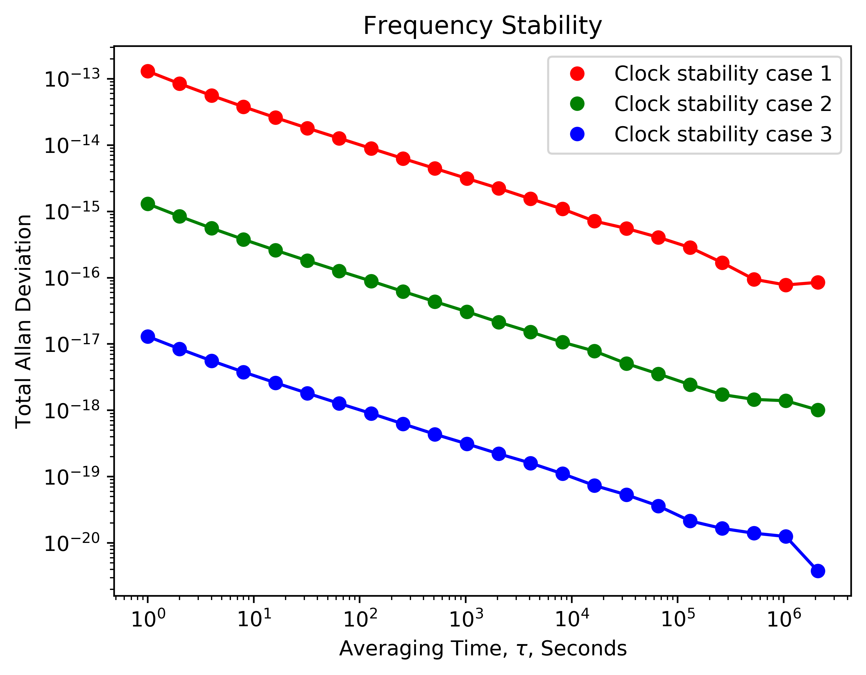
We first set the clock error magnitude of as , which is achievable currently. Considering the present best clocks with stability of in several hours, we reduce the magnitude of to and respectively to improve the observations. Although there are many kinds of random noises that affect Atomic clocks’ signals (Major, \APACyear2013), the most prominent components are white frequency modulation and random walk frequency modulation (Galleani \BOthers., \APACyear2003). Correspondingly the behaviors of clock errors are modeled as following equation
| (8) |
where , , and are constant coefficients, and are both standard white Gaussian noises. Each term in the right side of Eq.(8) has clear physical meaning; specifically denotes the initial frequency difference, is the drift term, is the white noise component, and represents the random walk effect. As we set proper values of constant coefficients in accordance with the performance of OACs in Oelker \BOthers. (\APACyear2019), a series of frequency comparison data with errors embedded can be generated. The statistic property of three clock error series are shown in Fig. 6.
Other error sources are discussed in detail in Z. Shen \BOthers. (\APACyear2017). Although Z. Shen \BOthers. (\APACyear2017) focus on the satellite to ground case, we can use similar methods to analyze the errors in the satellite to satellite case, and most of them demonstrate the same magnitude. The magnitudes of these error sources are listed in Table 2.
As for the mathematical model of these errors, we adopt a general error model which contains systematic (initial) offset, drift and white Gaussian noises for each of the error source, expressed as the following equation
| (9) |
where , and are constant coefficients, which are randomly set in accordance with the error magnitudes listed in Table 2
| Influence factor | (Residual) Error magnitude in |
|---|---|
| ionospheric correction residual | |
| tidal correction residual | |
| position & velocity | (10 mm and 0.1mm/s a) |
| clock error |
a Satellite’s position errors are assumed as 10 mm (Kang \BOthers., \APACyear2006), velocity errors are assumed as 0.1mm/s (Sharifi \BOthers., \APACyear2013);
According to Eqs. (8) and (9), we can generate the noise signals term in Eq. (7) based on the magnitudes and nature of the error sources at any time. Noted that the first 4 terms or the right side of Eq. (7) are true values, the 5th terms () is the corrections of ionosphere and tide effect. The values of these 5 terms can be directly calculated. Therefore we can get a set of relevant ”Observed” values, which constitute time series of TS’s gravitational potential as the left side of Eq. (7). Since the TS flies over the whole Earth in a period of about 30 d, these values are corresponding to the gravitational potential at different time points on the TS’s orbits and we obtain a set of values related to orbit data.
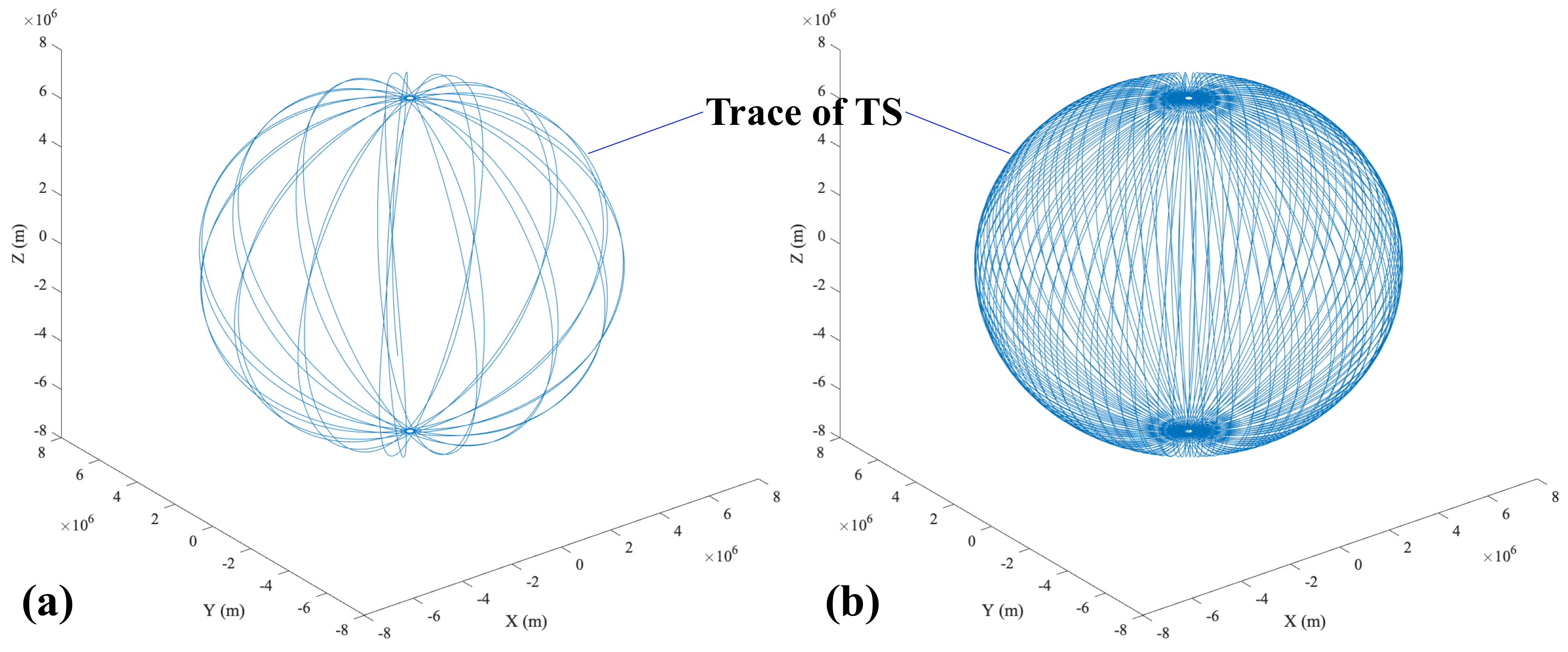
3.3 Determination of the GPD over the TSS
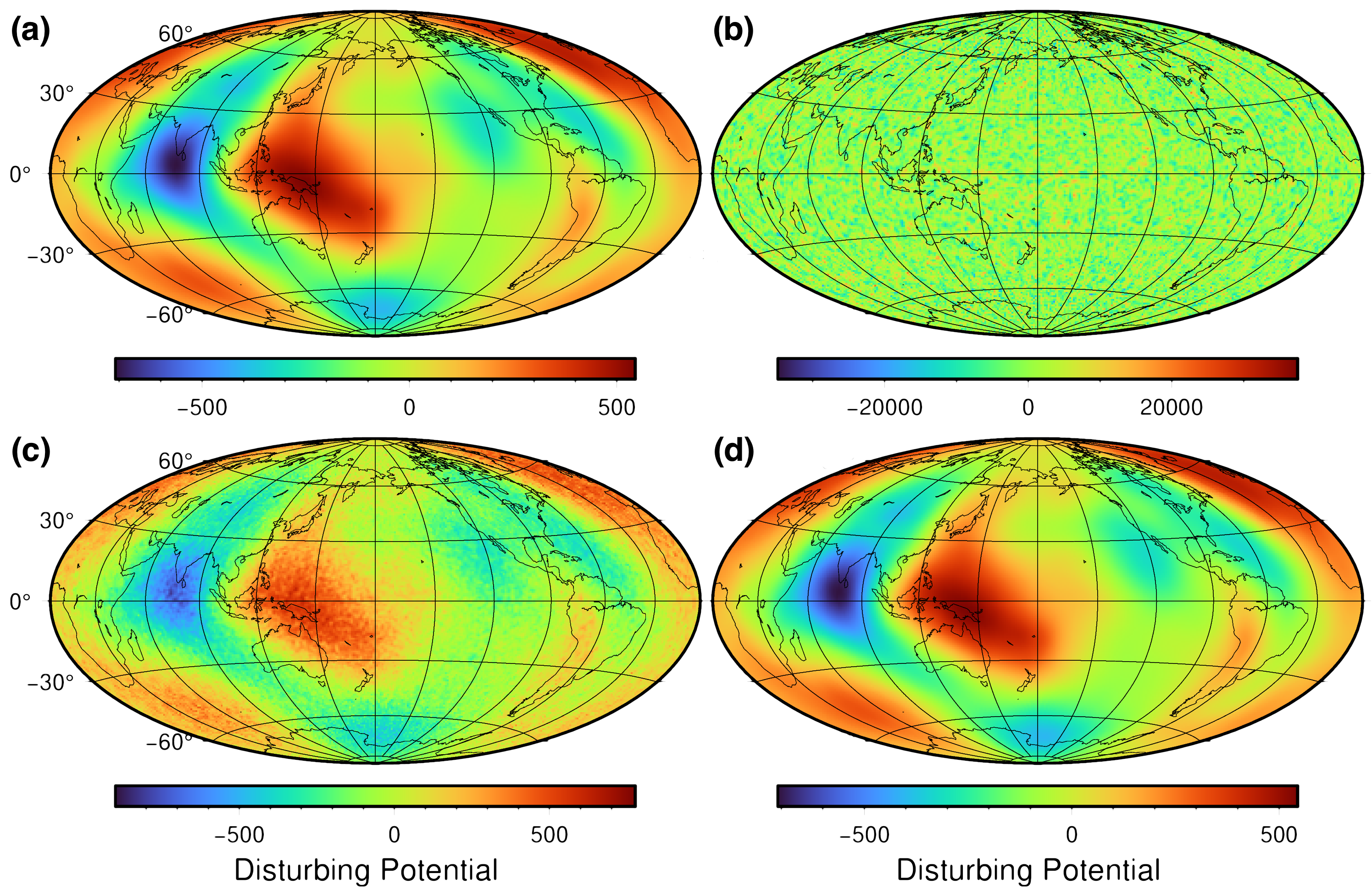
After a continuous observation of 30.0 days (720.0 hours), there are 324,000 observed GP points distributed over the TSS enclosing the Earth (see Fig. 7). The corresponding disturbing potentials of the three different experiment cases are depicted in Fig. 8, where the first subfigure demonstrates the disturbing potential of EGM2008 as true values. we can see that the observe results of case 1 (clock instability of ) seems to be useless, but the observe results of case 3 (clock instability of ) are almost identical with the true values. In the next section, we will calculate the spherical harmonic expansion coefficients for 3 different recovered Earths gravity field models (REGMs) based on the observed GP values in our simulation experiments. These coefficients will be compared with the true value of EGM2008 to evaluate their accuracy.
4 Determination of the Earth’s external gravitational potential field
Based on the determined GPD over the TDS using frequency links, we can determine the gravitational potential field outside the solid Earth by least-squares (LS) approach. The Earth’s gravitational potential at a point outside the Earth can be expanded into a series of spherical harmonics (Hofmann-Wellenhof \BBA Moritz, \APACyear2005)
| (10) |
where the spherical coordinates represent a 3-D position in the Earth-Centered, Earth-Fixed (ECEF) reference frame, is the geocentric radius, and are the spherical co-latitude and longitude respectively, is the geocentric gravitational constant, is the semi-major axis of the reference ellipsoid, and the (fully-normalized) geopotential coefficients which describe the external gravitational field of the Earth, are the (fully-normalized) associated Legendre functions of degree and order , and is the maximum degree of the harmonic expansion.
For the linear observation equation Eq. (10), the functional and statistical models of the gravitational field recovery from the GPD observations are defined by a standard Gauss-Markov model as follows:
| (11) |
where is the vector of GP observations, is the design matrix, is the vector of (unknown) geopotential coefficients to be estimated, is the vector of observation errors, is the error variance-covariance matrix, is the weight matrix, is the inverse of the weight matrix, and is the variance component.
Based on the data processing method described above, we estimated three REGMs up to degree and order 200 from GP values distributed over the TSS in three different cases, corresponding respectively the clock’s instabilities of , and . Here we set the weight matrix as a unit matrix by considering that the noise in GP observations is white noise. The absolute values of the coefficient differences (logarithm representation) between the recovered harmonic expansion coefficients of Earth’s gravity field and that of EGM2008 are illustrated globally in Fig. 9 as (a), (b) and (c).
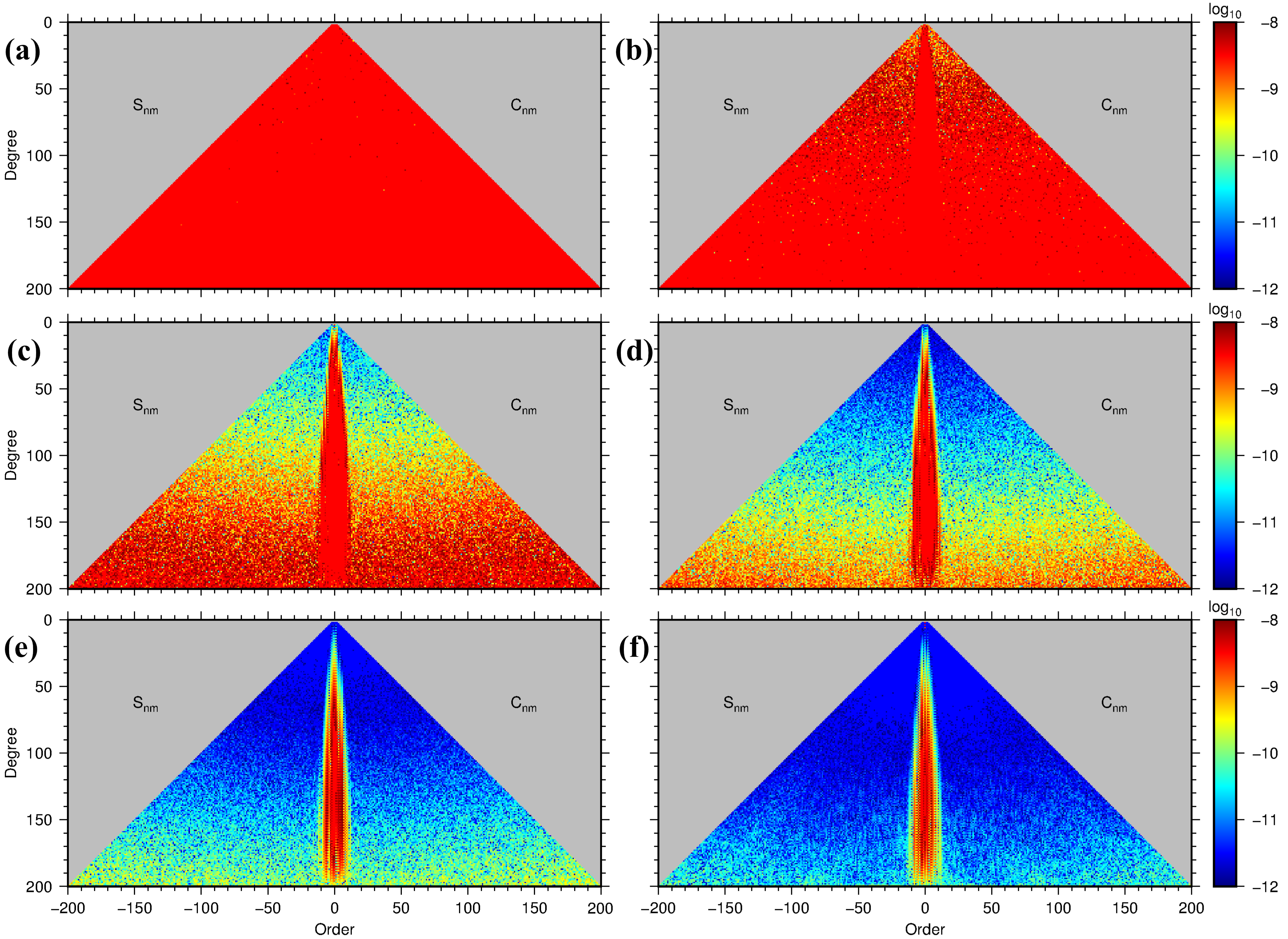
The results show that if the clock instability is poorer than (as cases (a) and (b)),the precision of recovered Earth’s gravity fields is poor. When the clock instability reach as case (c), we can obtain a fairly good coefficients for orders and degrees lower than 50. In addition, the zonal and near-zonal coefficients of REGMs are worse than other kinds of coefficients when the clock’s instability reaches . This is due to the fact that we did not use any regularized technique to deal with the ill-posed problem caused by the polar gap of GOCE mission. However, even if we use the regularized technique to deal with the ill-posed problem, the above mentioned problem still exists (Baur \BOthers., \APACyear2014).
The performance of REGMs can also be evaluated by the calculated GPs at the TSS (TS-orbit defined spherical surface). The mean offset and standard deviation (STD) of the calculated GP distribution difference between EGM2008 and REGMs over TSS are illustrated in Table 3. The STDs of GPD over the TSS are respectively 1135.3232 , 11.3758 and 0.114 for cases (a), (b) and (c).
| Case | Clock precision | Mean offset () | STD () |
|---|---|---|---|
| (a) | 0.9142 | 1135.3232 | |
| (b) | 0.2094 | 11.3758 | |
| (c) | -0.0009 | 0.1142 | |
| (d) | -0.0001 | 0.0114 | |
| (e) | -2.5e-6 | 0.0013 | |
| (f) | NA | 2.4e-8 | 0.0006 |
If the clock instabilities can be improved to or even level, some other error sources, such as ionospheric residual and velocity error, will take dominant and become the bottle neck for the precision of recovered coefficients. In that case, further detailed analysis or corrections for various error sources is required for establishing better correction models. Since there might be an extended period for us to set onboard clocks of instability level, in this paper we will leave that researches for future works. However, in order to show the potential of this method, we conducted two simplified experiments that The total error (the sum of clock errors and various other error sources) of SFST links are set to and respectively as illustrated in Fig. 9 (d) and (e). We can see that if the total error magnitudes can reduced to , the recovered harmonic expansion coefficients show fairly good quality, close to that recovered from the true values as illustrated in Fig. 9 (f). The REGM’s precision of case (d), (e) and (f) are shown in table 3.
5 Conclusion
In this paper we formulated an alternative method to determine satellite gravity field based on precise clocks and frequency signals transfer. It is a new application of general relativistic theory in geodesy, and the gravity field can be determined at the precision levels of about , and , given the clock stabilities of , and respectively. Currently the stability of a satellite’s onboard clock is about , and it is the main error influence for GP determination and EGM establishment. However, precise optical atomic clocks have reached level under laboratory environments (Oelker \BOthers., \APACyear2019). It is foreseeable that in the near future the stability of onboard atomic clocks can achieve a similar level, and the precision of the EGM established by intersatellite SFST method can reach 1 cm level. Compared to the conventionally used methods of establishing satellite gravity model such as using gravimeter and gravity gradiometer to measure the first-order and second-order derivative of potential, the SFST method may directly determine the GPs, simplifying in some sense the estimation of the harmonic coefficients of Earth’s gravity field.
According to this study, once the onboard clocks’ stabilities reach the level of , the relativistic method will be applicable for high precision satellite gravity field determination, and can be used to provide a decimeter level Earth gravity model with a resolution of around . If clock stabilities are better than ( or even for instance), various other error sources (ionosphere and troposphere correction residual errors, satellite position errors, et al.) will be the bottle-neck for determining a precise Earth’s gravity field, and more precise error correction models need to be established.
Acknowledgements.
This study is supported by National Natural Science Foundation of China (NSFC) (grant Nos. 41721003, 41631072, 41874023, 41804012, 41429401, 41574007), and Natural Science Foundation of Hubei Province (grant No. 2019CFB611).References
- Altschul \BOthers. (\APACyear2014) \APACinsertmetastarAltschul2014-og{APACrefauthors}Altschul, B., Bailey, Q\BPBIG., Blanchet, L., Bongs, K., Bouyer, P., Cacciapuoti, L.\BDBLWolf, P. \APACrefYearMonthDay2014\APACmonth01. \BBOQ\APACrefatitleQuantum Tests of the Einstein Equivalence Principle with the STE-QUEST Space Mission Quantum tests of the einstein equivalence principle with the STE-QUEST space mission.\BBCQ \APACjournalVolNumPagesAdv. Space Res.551501–524. \PrintBackRefs\CurrentBib
- Baur \BOthers. (\APACyear2014) \APACinsertmetastarBaur2014-oa{APACrefauthors}Baur, O., Bock, H., Höck, E., Jäggi, A., Krauss, S., Mayer-Gürr, T.\BDBLZehentner, N. \APACrefYearMonthDay2014\APACmonth10. \BBOQ\APACrefatitleComparison of GOCE-GPS gravity fields derived by different approaches Comparison of GOCE-GPS gravity fields derived by different approaches.\BBCQ \APACjournalVolNumPagesJ. Geodesy8810959–973. \PrintBackRefs\CurrentBib
- Bilitza \BOthers. (\APACyear2017) \APACinsertmetastarBilitza2017-zr{APACrefauthors}Bilitza, D., Altadill, D., Truhlik, V., Shubin, V., Galkin, I., Reinisch, B.\BCBL \BBA Huang, X. \APACrefYearMonthDay2017\APACmonth02. \BBOQ\APACrefatitleInternational reference ionosphere 2016: From ionospheric climate to real-time weather predictions International reference ionosphere 2016: From ionospheric climate to real-time weather predictions.\BBCQ \APACjournalVolNumPagesSpace Weather152418–429. \PrintBackRefs\CurrentBib
- Bjerhammar (\APACyear1985) \APACinsertmetastarBjerhammar1985-bd{APACrefauthors}Bjerhammar, A. \APACrefYearMonthDay1985\APACmonth01. \BBOQ\APACrefatitleOn a relativistic geodesy On a relativistic geodesy.\BBCQ \APACjournalVolNumPagesBull. Am. Assoc. Hist. Nurs.593207–220. \PrintBackRefs\CurrentBib
- Bock \BOthers. (\APACyear2011) \APACinsertmetastarBock2011-la{APACrefauthors}Bock, H., Jäggi, A., Meyer, U., Visser, P., van den IJssel, J., van Helleputte, T.\BDBLHugentobler, U. \APACrefYearMonthDay2011\APACmonth05. \BBOQ\APACrefatitleGPS-derived orbits for the GOCE satellite GPS-derived orbits for the GOCE satellite.\BBCQ \APACjournalVolNumPagesJ. Geodesy8511807–818. \PrintBackRefs\CurrentBib
- Croitoru \BBA Oancea (\APACyear2016) \APACinsertmetastarRomania2016-aa{APACrefauthors}Croitoru, E\BHBII.\BCBT \BBA Oancea, G. \APACrefYearMonthDay2016\APACmonth06. \BBOQ\APACrefatitleSatellite tracking using norad two-line element set format Satellite tracking using norad two-line element set format.\BBCQ \APACjournalVolNumPagesAFASES 2016181423–432. \PrintBackRefs\CurrentBib
- Deschênes \BOthers. (\APACyear2016) \APACinsertmetastarDeschenes2016-pr{APACrefauthors}Deschênes, J\BHBID., Sinclair, L\BPBIC., Giorgetta, F\BPBIR., Swann, W\BPBIC., Baumann, E., Bergeron, H.\BDBLNewbury, N\BPBIR. \APACrefYearMonthDay2016\APACmonth05. \BBOQ\APACrefatitleSynchronization of Distant Optical Clocks at the Femtosecond Level Synchronization of distant optical clocks at the femtosecond level.\BBCQ \APACjournalVolNumPagesPhys. Rev. X62021016. \PrintBackRefs\CurrentBib
- Ditmar \BBA Sluijs (\APACyear2004) \APACinsertmetastarDitmar2004-si{APACrefauthors}Ditmar, P.\BCBT \BBA Sluijs, A\BPBIA\BPBIv\BPBIE\BPBIv\BPBId. \APACrefYearMonthDay2004\APACmonth09. \BBOQ\APACrefatitleA technique for modeling the Earth’s gravity field on the basis of satellite accelerations A technique for modeling the earth’s gravity field on the basis of satellite accelerations.\BBCQ \APACjournalVolNumPagesJ. Geodesy78112–33. \PrintBackRefs\CurrentBib
- Drinkwater \BOthers. (\APACyear2003) \APACinsertmetastarDrinkwater2003-os{APACrefauthors}Drinkwater, M\BPBIR., Floberghagen, R., Haagmans, R., Muzi, D.\BCBL \BBA Popescu, A. \APACrefYearMonthDay2003. \BBOQ\APACrefatitleGOCE: ESA’s First Earth Explorer Core Mission GOCE: ESA’s first earth explorer core mission.\BBCQ \BIn G. Beutler, M\BPBIR. Drinkwater, R. Rummel\BCBL \BBA R. Von Steiger (\BEDS), \APACrefbtitleEarth Gravity Field from Space — From Sensors to Earth Sciences: Proceedings of an ISSI Workshop 11–15 March 2002, Bern, Switzerland Earth gravity field from space — from sensors to earth sciences: Proceedings of an ISSI workshop 11–15 march 2002, bern, switzerland (\BPGS 419–432). \APACaddressPublisherDordrechtSpringer Netherlands. \PrintBackRefs\CurrentBib
- Dziewonski \BBA Anderson (\APACyear1981) \APACinsertmetastarDziewonski1981-kj{APACrefauthors}Dziewonski, A\BPBIM.\BCBT \BBA Anderson, D\BPBIL. \APACrefYearMonthDay1981\APACmonth06. \BBOQ\APACrefatitlePreliminary reference Earth model Preliminary reference earth model.\BBCQ \APACjournalVolNumPagesPhys. Earth Planet. Inter.254297–356. \PrintBackRefs\CurrentBib
- Einstein (\APACyear1915) \APACinsertmetastarEinstein1915-tv{APACrefauthors}Einstein, A. \APACrefYearMonthDay1915\APACmonth01. \BBOQ\APACrefatitleDie Feldgleichungen der Gravitation Die feldgleichungen der gravitation.\BBCQ \APACjournalVolNumPagesSitzungsberichte der Königlich Preußischen Akademie der Wissenschaften (Berlin), Seite 844-847.1844–847. \PrintBackRefs\CurrentBib
- Flechtner \BOthers. (\APACyear2016) \APACinsertmetastarFlechtner2016-jp{APACrefauthors}Flechtner, F., Neumayer, K\BHBIH., Dahle, C., Dobslaw, H., Fagiolini, E., Raimondo, J\BHBIC.\BCBL \BBA Güntner, A. \APACrefYearMonthDay2016\APACmonth03. \BBOQ\APACrefatitleWhat Can be Expected from the GRACE-FO Laser Ranging Interferometer for Earth Science Applications? What can be expected from the GRACE-FO laser ranging interferometer for earth science applications?\BBCQ \APACjournalVolNumPagesSurv. Geophys.372453–470. \PrintBackRefs\CurrentBib
- Flury (\APACyear2016) \APACinsertmetastarFlury2016-bw{APACrefauthors}Flury, J. \APACrefYearMonthDay2016\APACmonth07. \BBOQ\APACrefatitleRelativistic geodesy Relativistic geodesy.\BBCQ \APACjournalVolNumPagesJ. Phys. Conf. Ser.7231012051. \PrintBackRefs\CurrentBib
- Galleani \BOthers. (\APACyear2003) \APACinsertmetastarGalleani2003-hu{APACrefauthors}Galleani, L., Sacerdote, L., Tavella, P.\BCBL \BBA Zucca, C. \APACrefYearMonthDay2003\APACmonth06. \BBOQ\APACrefatitleA mathematical model for the atomic clock error A mathematical model for the atomic clock error.\BBCQ \APACjournalVolNumPagesMetrologia403S257. \PrintBackRefs\CurrentBib
- Grotti \BOthers. (\APACyear2018) \APACinsertmetastarGrotti2018-ap{APACrefauthors}Grotti, J., Koller, S., Vogt, S., Häfner, S., Sterr, U., Lisdat, C.\BDBLCalonico, D. \APACrefYearMonthDay2018\APACmonth05. \BBOQ\APACrefatitleGeodesy and metrology with a transportable optical clock Geodesy and metrology with a transportable optical clock.\BBCQ \APACjournalVolNumPagesNat. Phys.145437–441. \PrintBackRefs\CurrentBib
- Han \BOthers. (\APACyear2002) \APACinsertmetastarHan2002-oe{APACrefauthors}Han, S\BHBIC., Jekeli, C.\BCBL \BBA Shum, C\BPBIK. \APACrefYearMonthDay2002\APACmonth08. \BBOQ\APACrefatitleEfficient gravity field recovery using in situ disturbing potential observables from CHAMP: GRAVITY FIELD RECOVERY FROM CHAMP Efficient gravity field recovery using in situ disturbing potential observables from CHAMP: GRAVITY FIELD RECOVERY FROM CHAMP.\BBCQ \APACjournalVolNumPagesGeophys. Res. Lett.291636–1–36–4. \PrintBackRefs\CurrentBib
- Hannig \BOthers. (\APACyear2019) \APACinsertmetastarHannig2019-yh{APACrefauthors}Hannig, S., Pelzer, L., Scharnhorst, N., Kramer, J., Stepanova, M., Xu, Z\BPBIT.\BDBLSchmidt, P\BPBIO. \APACrefYearMonthDay2019\APACmonth05. \BBOQ\APACrefatitleTowards a transportable aluminium ion quantum logic optical clock Towards a transportable aluminium ion quantum logic optical clock.\BBCQ \APACjournalVolNumPagesRev. Sci. Instrum.905053204. \PrintBackRefs\CurrentBib
- Heiskanen \BBA Moritz (\APACyear1967) \APACinsertmetastarHeiskanen1967-ue{APACrefauthors}Heiskanen, W\BPBIA.\BCBT \BBA Moritz, H. \APACrefYearMonthDay1967\APACmonth12. \BBOQ\APACrefatitlePhysical geodesy Physical geodesy.\BBCQ \APACjournalVolNumPagesBull. Geodesique861491–492. \PrintBackRefs\CurrentBib
- Hirt \BOthers. (\APACyear2012) \APACinsertmetastarHirt2012-yg{APACrefauthors}Hirt, C., Kuhn, M., Featherstone, W\BPBIE.\BCBL \BBA Göttl, F. \APACrefYearMonthDay2012\APACmonth05. \BBOQ\APACrefatitleTopographic/isostatic evaluation of new-generation GOCE gravity field models: TOPOISOSTATIC EVALUATION OF GOCE GRAVITY Topographic/isostatic evaluation of new-generation GOCE gravity field models: TOPOISOSTATIC EVALUATION OF GOCE GRAVITY.\BBCQ \APACjournalVolNumPagesJ. Geophys. Res.117B5. \PrintBackRefs\CurrentBib
- Hofmann-Wellenhof \BBA Moritz (\APACyear2005) \APACinsertmetastarHofmann-Wellenhof2005-ur{APACrefauthors}Hofmann-Wellenhof, B.\BCBT \BBA Moritz, H. \APACrefYear2005. \APACrefbtitlePhysical geodesy Physical geodesy. \APACaddressPublisherSpringer. \PrintBackRefs\CurrentBib
- Huang \BOthers. (\APACyear2019) \APACinsertmetastarHuang2019-ez{APACrefauthors}Huang, Y., Guan, H., Zeng, M., Tang, L.\BCBL \BBA Gao, K. \APACrefYearMonthDay2019\APACmonth01. \BBOQ\APACrefatitle40Ca+ ion optical clock with micromotion-induced shifts below 10-18 40Ca+ ion optical clock with micromotion-induced shifts below 10-18.\BBCQ \APACjournalVolNumPagesPhys. Rev. A991011401. \PrintBackRefs\CurrentBib
- Hwang (\APACyear2001) \APACinsertmetastarHwang2001-jc{APACrefauthors}Hwang, C. \APACrefYearMonthDay2001\APACmonth05. \BBOQ\APACrefatitleGravity recovery using COSMIC GPS data: application of orbital perturbation theory Gravity recovery using COSMIC GPS data: application of orbital perturbation theory.\BBCQ \APACjournalVolNumPagesJ. Geodesy752117–136. \PrintBackRefs\CurrentBib
- Jekeli (\APACyear1999) \APACinsertmetastarJekeli1999-gr{APACrefauthors}Jekeli, C. \APACrefYearMonthDay1999\APACmonth10. \BBOQ\APACrefatitleThe determination of gravitational potential differences from satellite-to-satellite tracking The determination of gravitational potential differences from satellite-to-satellite tracking.\BBCQ \APACjournalVolNumPagesCelest. Mech. Dyn. Astron.75285–101. \PrintBackRefs\CurrentBib
- Kang \BOthers. (\APACyear2006) \APACinsertmetastarKang2006-ix{APACrefauthors}Kang, Z., Tapley, B., Bettadpur, S., Ries, J., Nagel, P.\BCBL \BBA Pastor, R. \APACrefYearMonthDay2006\APACmonth01. \BBOQ\APACrefatitlePrecise orbit determination for the GRACE mission using only GPS data Precise orbit determination for the GRACE mission using only GPS data.\BBCQ \APACjournalVolNumPagesJ. Geodesy806322–331. \PrintBackRefs\CurrentBib
- Kaula (\APACyear1966) \APACinsertmetastarKaula1966-ke{APACrefauthors}Kaula, W\BPBIM. \APACrefYear1966. \APACrefbtitleTheory of Satellite Geodesy: Applications of Satellites to Geodesy Theory of satellite geodesy: Applications of satellites to geodesy. \APACaddressPublisherDover Publications. \PrintBackRefs\CurrentBib
- Kleppner \BOthers. (\APACyear1970) \APACinsertmetastarKleppner1970-db{APACrefauthors}Kleppner, D., Vessot, R\BPBIF\BPBIC.\BCBL \BBA Ramsey, N\BPBIF. \APACrefYearMonthDay1970\APACmonth01. \BBOQ\APACrefatitleAn orbiting clock experiment to determine the gravitational red shift An orbiting clock experiment to determine the gravitational red shift.\BBCQ \APACjournalVolNumPagesAstrophys. Space Sci.6113–32. \PrintBackRefs\CurrentBib
- Kopeikin \BOthers. (\APACyear2016) \APACinsertmetastarKopeikin2016-dk{APACrefauthors}Kopeikin, S\BPBIM., Kanushin, V\BPBIF., Karpik, A\BPBIP., Tolstikov, A\BPBIS., Gienko, E\BPBIG., Goldobin, D\BPBIN.\BDBLHanikova, E\BPBIA. \APACrefYearMonthDay2016\APACmonth07. \BBOQ\APACrefatitleChronometric measurement of orthometric height differences by means of atomic clocks Chronometric measurement of orthometric height differences by means of atomic clocks.\BBCQ \APACjournalVolNumPagesGravitation Cosmol.223234–244. \PrintBackRefs\CurrentBib
- Kornfeld \BOthers. (\APACyear2019) \APACinsertmetastarKornfeld2019-er{APACrefauthors}Kornfeld, R\BPBIP., Arnold, B\BPBIW., Gross, M\BPBIA., Dahya, N\BPBIT., Klipstein, W\BPBIM., Gath, P\BPBIF.\BCBL \BBA Bettadpur, S. \APACrefYearMonthDay2019\APACmonth05. \BBOQ\APACrefatitleGRACE-FO: The Gravity Recovery and Climate Experiment Follow-On Mission GRACE-FO: The gravity recovery and climate experiment Follow-On mission.\BBCQ \APACjournalVolNumPagesJ. Spacecr. Rockets563931–951. \PrintBackRefs\CurrentBib
- Kvas \BBA Mayer-Gürr (\APACyear2019) \APACinsertmetastarKvas2019-vj{APACrefauthors}Kvas, A.\BCBT \BBA Mayer-Gürr, T. \APACrefYearMonthDay2019\APACmonth12. \BBOQ\APACrefatitleGRACE gravity field recovery with background model uncertainties GRACE gravity field recovery with background model uncertainties.\BBCQ \APACjournalVolNumPagesJ. Geodesy93122543–2552. \PrintBackRefs\CurrentBib
- Laurent \BOthers. (\APACyear2015) \APACinsertmetastarLaurent2015-ly{APACrefauthors}Laurent, P., Massonnet, D., Cacciapuoti, L.\BCBL \BBA Salomon, C. \APACrefYearMonthDay2015. \BBOQ\APACrefatitleThe ACES/PHARAO space mission The ACES/PHARAO space mission.\BBCQ \APACjournalVolNumPagesC. R. Phys.165540–552. \PrintBackRefs\CurrentBib
- Liu \BOthers. (\APACyear2018) \APACinsertmetastarLiu2018-oo{APACrefauthors}Liu, L., Lü, D\BHBIS., Chen, W\BHBIB., Li, T., Qu, Q\BHBIZ., Wang, B.\BDBLWang, Y\BHBIZ. \APACrefYearMonthDay2018\APACmonth07. \BBOQ\APACrefatitleIn-orbit operation of an atomic clock based on laser-cooled 87Rb atoms In-orbit operation of an atomic clock based on laser-cooled 87rb atoms.\BBCQ \APACjournalVolNumPagesNat. Commun.912760. \PrintBackRefs\CurrentBib
- Major (\APACyear2013) \APACinsertmetastarMajor2013-qc{APACrefauthors}Major, F\BPBIG. \APACrefYear2013. \APACrefbtitleThe Quantum Beat: The Physical Principles of Atomic Clocks The quantum beat: The physical principles of atomic clocks. \APACaddressPublisherSpringer Science & Business Media. \PrintBackRefs\CurrentBib
- McGrew \BOthers. (\APACyear2018) \APACinsertmetastarMcGrew2018-og{APACrefauthors}McGrew, W\BPBIF., Zhang, X., Fasano, R\BPBIJ., Schäffer, S\BPBIA., Beloy, K., Nicolodi, D.\BDBLLudlow, A\BPBID. \APACrefYearMonthDay2018\APACmonth12. \BBOQ\APACrefatitleAtomic clock performance enabling geodesy below the centimetre level Atomic clock performance enabling geodesy below the centimetre level.\BBCQ \APACjournalVolNumPagesNature564773487–90. \PrintBackRefs\CurrentBib
- Mehlstäubler \BOthers. (\APACyear2018) \APACinsertmetastarMehlstaubler2018-da{APACrefauthors}Mehlstäubler, T\BPBIE., Grosche, G., Lisdat, C., Schmidt, P\BPBIO.\BCBL \BBA Denker, H. \APACrefYearMonthDay2018\APACmonth06. \BBOQ\APACrefatitleAtomic clocks for geodesy Atomic clocks for geodesy.\BBCQ \APACjournalVolNumPagesRep. Prog. Phys.816064401. \PrintBackRefs\CurrentBib
- Namazov \BOthers. (\APACyear1975) \APACinsertmetastarNamazov1975-qa{APACrefauthors}Namazov, S\BPBIA., Novikov, V\BPBID.\BCBL \BBA Khmel’nitskii, I\BPBIA. \APACrefYearMonthDay1975\APACmonth04. \BBOQ\APACrefatitleDoppler frequency shift during ionospheric propagation of decameter radio waves (review) Doppler frequency shift during ionospheric propagation of decameter radio waves (review).\BBCQ \APACjournalVolNumPagesRadiophys. Quantum Electron.184345–364. \PrintBackRefs\CurrentBib
- Oelker \BOthers. (\APACyear2019) \APACinsertmetastarOelker2019-wm{APACrefauthors}Oelker, E., Hutson, R\BPBIB., Kennedy, C\BPBIJ., Sonderhouse, L., Bothwell, T., Goban, A.\BDBLYe, J. \APACrefYearMonthDay2019\APACmonth10. \BBOQ\APACrefatitleDemonstration of stability at 1 s for two independent optical clocks Demonstration of stability at 1 s for two independent optical clocks.\BBCQ \APACjournalVolNumPagesNat. Photonics1310714–719. \PrintBackRefs\CurrentBib
- Pail \BOthers. (\APACyear2011) \APACinsertmetastarPail2011-qy{APACrefauthors}Pail, R., Bruinsma, S., Migliaccio, F., Förste, C., Goiginger, H., Schuh, W\BHBID.\BDBLTscherning, C\BPBIC. \APACrefYearMonthDay2011\APACmonth11. \BBOQ\APACrefatitleFirst GOCE gravity field models derived by three different approaches First GOCE gravity field models derived by three different approaches.\BBCQ \APACjournalVolNumPagesJ Geod8511819. \PrintBackRefs\CurrentBib
- Pail \BOthers. (\APACyear2019) \APACinsertmetastarPail2019-ao{APACrefauthors}Pail, R., Yeh, H\BHBIC., Feng, W., Hauk, M., Purkhauser, A., Wang, C.\BDBLXu, H. \APACrefYearMonthDay2019\APACmonth11. \BBOQ\APACrefatitleNext-Generation Gravity Missions: Sino-European Numerical Simulation Comparison Exercise Next-Generation gravity missions: Sino-European numerical simulation comparison exercise.\BBCQ \APACjournalVolNumPagesRemote Sensing11222654. \PrintBackRefs\CurrentBib
- Pavlis \BOthers. (\APACyear2012) \APACinsertmetastarPavlis2012-fw{APACrefauthors}Pavlis, N\BPBIK., Holmes, S\BPBIA., Kenyon, S\BPBIC.\BCBL \BBA others. \APACrefYearMonthDay2012. \BBOQ\APACrefatitleThe development and evaluation of the Earth Gravitational Model 2008 (EGM2008) The development and evaluation of the earth gravitational model 2008 (EGM2008).\BBCQ \APACjournalVolNumPagesJournal of Geophysical Research: Solid Earth117B4B04406. \PrintBackRefs\CurrentBib
- Pierno \BBA Varasi (\APACyear2013) \APACinsertmetastarPierno2013-ub{APACrefauthors}Pierno, L.\BCBT \BBA Varasi, M. \APACrefYearMonthDay2013\APACmonth06. \APACrefbtitleSwitchable delays optical fibre transponder with optical generation of doppler shift Switchable delays optical fibre transponder with optical generation of doppler shift (\BNUM 8466831). \PrintBackRefs\CurrentBib
- Puetzfeld \BBA Lämmerzahl (\APACyear2019) \APACinsertmetastarPuetzfeld2019-sl{APACrefauthors}Puetzfeld, D.\BCBT \BBA Lämmerzahl, C. (\BEDS). \APACrefYear2019. \APACrefbtitleRelativistic Geodesy: Foundations and Applications Relativistic geodesy: Foundations and applications. \APACaddressPublisherSpringer, Cham. \PrintBackRefs\CurrentBib
- Rawer \BOthers. (\APACyear1978) \APACinsertmetastarRawer1978-fl{APACrefauthors}Rawer, K., Bilitza, D.\BCBL \BBA Ramakrishnan, S. \APACrefYearMonthDay1978. \BBOQ\APACrefatitleGoals and status of the International Reference Ionosphere Goals and status of the international reference ionosphere.\BBCQ \APACjournalVolNumPagesRev. Geophys.162177. \PrintBackRefs\CurrentBib
- Reigber \BOthers. (\APACyear2002) \APACinsertmetastarReigber2002-uf{APACrefauthors}Reigber, C., Balmino, G., Schwintzer, P., Biancale, R., Bode, A., Lemoine, J\BHBIM.\BDBLZhu, S\BPBIY. \APACrefYearMonthDay2002\APACmonth07. \BBOQ\APACrefatitleA high-quality global gravity field model from CHAMP GPS tracking data and accelerometry (EIGEN-1S): A GLOBAL GRAVITY FIELD MODEL A high-quality global gravity field model from CHAMP GPS tracking data and accelerometry (EIGEN-1S): A GLOBAL GRAVITY FIELD MODEL.\BBCQ \APACjournalVolNumPagesGeophys. Res. Lett.291437–1–37–4. \PrintBackRefs\CurrentBib
- Reubelt \BOthers. (\APACyear2003) \APACinsertmetastarReubelt2003-yb{APACrefauthors}Reubelt, T., Austen, G.\BCBL \BBA Grafarend, E\BPBIW. \APACrefYearMonthDay2003\APACmonth08. \BBOQ\APACrefatitleHarmonic analysis of the Earth’s gravitational field by means of semi-continuous ephemerides of a low Earth orbiting GPS-tracked satellite. Case study: CHAMP Harmonic analysis of the earth’s gravitational field by means of semi-continuous ephemerides of a low earth orbiting GPS-tracked satellite. case study: CHAMP.\BBCQ \APACjournalVolNumPagesJ. Geodesy775257–278. \PrintBackRefs\CurrentBib
- Schiller \BOthers. (\APACyear2012) \APACinsertmetastarSchiller2012-ps{APACrefauthors}Schiller, S., Gorlitz, A., Nevsky, A., Alighanbari, S., Vasilyev, S., Abou-Jaoudeh, C.\BDBLLevi, F. \APACrefYearMonthDay2012\APACmonth04. \BBOQ\APACrefatitleThe space optical clocks project: Development of high-performance transportable and breadboard optical clocks and advanced subsystems The space optical clocks project: Development of high-performance transportable and breadboard optical clocks and advanced subsystems.\BBCQ \BIn \APACrefbtitle2012 European Frequency and Time Forum 2012 european frequency and time forum (\BPGS 412–418). \APACaddressPublisherIEEE. \PrintBackRefs\CurrentBib
- Sharifi \BOthers. (\APACyear2013) \APACinsertmetastarSharifi2013-bm{APACrefauthors}Sharifi, M\BPBIA., Seif, M\BPBIR.\BCBL \BBA Hadi, M\BPBIA. \APACrefYearMonthDay2013. \BBOQ\APACrefatitleA Comparison Between Numerical Differentiation and Kalman Filtering for a Leo Satellite Velocity Determination A comparison between numerical differentiation and kalman filtering for a leo satellite velocity determination.\BBCQ \APACjournalVolNumPagesArtificial Satellites483103–110. \PrintBackRefs\CurrentBib
- W. Shen \BOthers. (\APACyear2011) \APACinsertmetastarShen2011-fm{APACrefauthors}Shen, W., Ning, J., Liu, J., Li, J.\BCBL \BBA Chao, D. \APACrefYearMonthDay2011\APACmonth01. \BBOQ\APACrefatitleDetermination of the geopotential and orthometric height based on frequency shift equation Determination of the geopotential and orthometric height based on frequency shift equation.\BBCQ \APACjournalVolNumPagesNat. Sci.35388–396. \PrintBackRefs\CurrentBib
- Z. Shen \BOthers. (\APACyear2018) \APACinsertmetastarShen2018-jq{APACrefauthors}Shen, Z., Shen, W.\BCBL \BBA Zhang, S. \APACrefYearMonthDay2018\APACmonth04. \BBOQ\APACrefatitleDetermination of the gravitational potential at GOCE-type satellite orbit using frequency signal transmission approach Determination of the gravitational potential at GOCE-type satellite orbit using frequency signal transmission approach.\BBCQ \BIn \APACrefbtitle20st EGU General Assembly, EGU2018 20st EGU general assembly, EGU2018 (\BPG 19415). \PrintBackRefs\CurrentBib
- Z. Shen, Shen\BCBL \BBA Zhang (\APACyear2019) \APACinsertmetastarShen2019-hk{APACrefauthors}Shen, Z., Shen, W.\BCBL \BBA Zhang, S. \APACrefYearMonthDay2019\APACmonth04. \BBOQ\APACrefatitleDetermination of gravitational potential distribution over a geocentric quasi-sphere based on satellite-to-satellite frequency transmitting Determination of gravitational potential distribution over a geocentric quasi-sphere based on satellite-to-satellite frequency transmitting.\BBCQ \BIn \APACrefbtitle21st EGU General Assembly, EGU2019 21st EGU general assembly, EGU2019 (\BPG 4591). \PrintBackRefs\CurrentBib
- Z. Shen \BBA Shen (\APACyear2017) \APACinsertmetastarShen2017-xg{APACrefauthors}Shen, Z.\BCBT \BBA Shen, W\BHBIB. \APACrefYearMonthDay2017. \BBOQ\APACrefatitleDetermination of gravitational potential distribution over a geocentric quasi- sphere based on links between GRACE- and GNSS-type satellites Determination of gravitational potential distribution over a geocentric quasi- sphere based on links between GRACE- and GNSS-type satellites.\BBCQ \BIn \APACrefbtitle19th EGU General Assembly, EGU2017 19th EGU general assembly, EGU2017 (\BPG 11250). \PrintBackRefs\CurrentBib
- Z. Shen, Shen, Peng\BCBL \BOthers. (\APACyear2019) \APACinsertmetastarShen2019-od{APACrefauthors}Shen, Z., Shen, W\BHBIB., Peng, Z., Liu, T., Zhang, S.\BCBL \BBA Chao, D. \APACrefYearMonthDay2019\APACmonth04. \BBOQ\APACrefatitleFormulation of Determining the Gravity Potential Difference Using Ultra-High Precise Clocks via Optical Fiber Frequency Transfer Technique Formulation of determining the gravity potential difference using Ultra-High precise clocks via optical fiber frequency transfer technique.\BBCQ \APACjournalVolNumPagesJ. Earth Sci.302422–428. \PrintBackRefs\CurrentBib
- Z. Shen \BOthers. (\APACyear2016) \APACinsertmetastarShen2016-lc{APACrefauthors}Shen, Z., Shen, W\BHBIB.\BCBL \BBA Zhang, S. \APACrefYearMonthDay2016\APACmonth08. \BBOQ\APACrefatitleFormulation of geopotential difference determination using optical-atomic clocks onboard satellites and on ground based on Doppler cancellation system Formulation of geopotential difference determination using optical-atomic clocks onboard satellites and on ground based on doppler cancellation system.\BBCQ \APACjournalVolNumPagesGeophys. J. Int.20621162–1168. \PrintBackRefs\CurrentBib
- Z. Shen \BOthers. (\APACyear2017) \APACinsertmetastarShen2017-kg{APACrefauthors}Shen, Z., Shen, W\BHBIB.\BCBL \BBA Zhang, S. \APACrefYearMonthDay2017\APACmonth07. \BBOQ\APACrefatitleDetermination of Gravitational Potential at Ground Using Optical-Atomic Clocks on Board Satellites and on Ground Stations and Relevant Simulation Experiments Determination of gravitational potential at ground using Optical-Atomic clocks on board satellites and on ground stations and relevant simulation experiments.\BBCQ \APACjournalVolNumPagesSurv. Geophys.384757–780. \PrintBackRefs\CurrentBib
- Takano \BOthers. (\APACyear2016) \APACinsertmetastarTakano2016-dr{APACrefauthors}Takano, T., Takamoto, M., Ushijima, I., Ohmae, N., Akatsuka, T., Yamaguchi, A.\BDBLKatori, H. \APACrefYearMonthDay2016\APACmonth08. \BBOQ\APACrefatitleGeopotential measurements with synchronously linked optical lattice clocks Geopotential measurements with synchronously linked optical lattice clocks.\BBCQ \APACjournalVolNumPagesNat. Photonics1010662. \PrintBackRefs\CurrentBib
- Tapley \BOthers. (\APACyear2004) \APACinsertmetastarTapley2004-tc{APACrefauthors}Tapley, B\BPBID., Bettadpur, S., Watkins, M.\BCBL \BBA Reigber, C. \APACrefYearMonthDay2004\APACmonth05. \BBOQ\APACrefatitleThe gravity recovery and climate experiment: Mission overview and early results: GRACE MISSION OVERVIEW AND EARLY RESULTS The gravity recovery and climate experiment: Mission overview and early results: GRACE MISSION OVERVIEW AND EARLY RESULTS.\BBCQ \APACjournalVolNumPagesGeophys. Res. Lett.319L09607. \PrintBackRefs\CurrentBib
- Van Camp \BBA Vauterin (\APACyear2005) \APACinsertmetastarVan_Camp2005-qt{APACrefauthors}Van Camp, M.\BCBT \BBA Vauterin, P. \APACrefYearMonthDay2005\APACmonth06. \BBOQ\APACrefatitleTsoft: graphical and interactive software for the analysis of time series and Earth tides Tsoft: graphical and interactive software for the analysis of time series and earth tides.\BBCQ \APACjournalVolNumPagesComput. Geosci.315631–640. \PrintBackRefs\CurrentBib
- Vessot \BBA Levine (\APACyear1979) \APACinsertmetastarVessot1979-ot{APACrefauthors}Vessot, R\BPBIF\BPBIC.\BCBT \BBA Levine, M\BPBIW. \APACrefYearMonthDay1979\APACmonth02. \BBOQ\APACrefatitleA test of the equivalence principle using a space-borne clock A test of the equivalence principle using a space-borne clock.\BBCQ \APACjournalVolNumPagesGen. Relat. Grav.103181–204. \PrintBackRefs\CurrentBib
- Vessot \BOthers. (\APACyear1980) \APACinsertmetastarVessot1980-ax{APACrefauthors}Vessot, R\BPBIF\BPBIC., Levine, M\BPBIW., Mattison, E\BPBIM., Blomberg, E\BPBIL., Hoffman, T\BPBIE., Nystrom, G\BPBIU.\BDBLWills, F\BPBID. \APACrefYearMonthDay1980\APACmonth12. \BBOQ\APACrefatitleTest of Relativistic Gravitation with a Space-Borne Hydrogen Maser Test of relativistic gravitation with a Space-Borne hydrogen maser.\BBCQ \APACjournalVolNumPagesPhys. Rev. Lett.45262081–2084. \PrintBackRefs\CurrentBib
- Visser \BOthers. (\APACyear2003) \APACinsertmetastarVisser2003-xw{APACrefauthors}Visser, P\BPBIN\BPBIA\BPBIM., Sneeuw, N.\BCBL \BBA Gerlach, C. \APACrefYearMonthDay2003\APACmonth06. \BBOQ\APACrefatitleEnergy integral method for gravity field determination from satellite orbit coordinates Energy integral method for gravity field determination from satellite orbit coordinates.\BBCQ \APACjournalVolNumPagesJ. Geodesy773207–216. \PrintBackRefs\CurrentBib
- Voigt \BOthers. (\APACyear2017) \APACinsertmetastarVoigt2017-qc{APACrefauthors}Voigt, C., Förste, C., Wziontek, H., Crossley, D., Meurers, B., Pálinkáš, V.\BDBLSun, H. \APACrefYearMonthDay2017. \BBOQ\APACrefatitleThe Data Base of the International Geodynamics and Earth Tide Service (IGETS) The data base of the international geodynamics and earth tide service (IGETS).\BBCQ \BIn \APACrefbtitle19th EGU General Assembly, EGU2017 19th EGU general assembly, EGU2017 (\BPG 4947). \PrintBackRefs\CurrentBib
- Weinberg (\APACyear1972) \APACinsertmetastarWeinberg1972-le{APACrefauthors}Weinberg, S. \APACrefYear1972. \APACrefbtitleGravitation and Cosmology: Principles and Applications of the General Theory of Relativity Gravitation and cosmology: Principles and applications of the general theory of relativity. \APACaddressPublisherNew YorkWiley. \PrintBackRefs\CurrentBib
- Wenzel (\APACyear1996) \APACinsertmetastarWenzel1996-tk{APACrefauthors}Wenzel, H\BHBIG. \APACrefYearMonthDay1996. \BBOQ\APACrefatitleThe nanogal software: Earth tide data processing package ETERNA 3.30 The nanogal software: Earth tide data processing package ETERNA 3.30.\BBCQ \APACjournalVolNumPagesBull. Inf. Marées Terrestres1249425–9439. \PrintBackRefs\CurrentBib
- Wu \BOthers. (\APACyear2019) \APACinsertmetastarWu2019-wq{APACrefauthors}Wu, H., Müller, J.\BCBL \BBA Lämmerzahl, C. \APACrefYearMonthDay2019\APACmonth03. \BBOQ\APACrefatitleClock networks for height system unification: a simulation study Clock networks for height system unification: a simulation study.\BBCQ \APACjournalVolNumPagesGeophys. J. Int.21631594–1607. \PrintBackRefs\CurrentBib