Identification of Time-Varying Transformation Models with Fixed Effects, with an Application to Unobserved Heterogeneity in Resource Shares

Abstract

We provide new results showing identification of a large class of fixed-$T$ panel models, where the response variable is an unknown, weakly monotone, time-varying transformation of a latent linear index of fixed effects, regressors, and an error term drawn from an unknown stationary distribution. Our results identify the transformation, the coefficient on regressors, and features of the distribution of the fixed effects. We then develop a full-commitment intertemporal collective household model, where the implied quantity demand equations are time-varying functions of a linear index. The fixed effects in this index equal logged resource shares, defined as the fractions of household expenditure enjoyed by each household member. Using Bangladeshi data, we show that women’s resource shares decline with household budgets and that half of the variation in women’s resource shares is due to unobserved household-level heterogeneity.

1 Introduction

We provide sufficient conditions for point-identification in a general class of fixed-$T$ time-varying nonlinear panel models. This class has a response variable equal to a time-varying weakly monotonic transformation of a linear index of regressors, fixed effects, and error terms. In contrast, almost all existing results for this class of models require time-invariance of the transformation. Our theorems imply novel identification results for time-varying versions of some commonly used models.

Specifically, we consider models of the type:

$$Y_{it}=h_{t}(\alpha_{i}+X_{it}\beta-U_{it}),i=1,\dots,n,\,t=1,\dots,T\geq 2,$$ (1.1)

where $h_{t}$ is an unknown weakly monotonic transformation, $\alpha_{i}$ are unobserved individual-specific effects, $X_{it}$ is a vector of strictly exogenous observed explanatory variables with coefficients $\beta$, and $U_{it}$ is an error term drawn from a stationary distribution.

Our setting has the following four features:

1. fixed-$T$ —in fact $T=2$ is sufficient for our results;

2. $h_{t}$ may be time-varying and weakly monotonic;

3. $h_{t}$ and the distribution of $U_{it}$ may be nonparametric;

4. and, the fixed effects $\alpha_{i}$ are unrestricted.

The panel model literature is very large, with many papers showing identification of $\beta$, and sometimes of $h_{t}$, in models with two or three of the four features above (see, e.g., Arellano and Bonhomme, (2011) for an overview). Ours is the first paper to study identification of models with these four features, all of which are demanded by our microeconomic model and empirical application. We refer to (1.1) together with the four features above as the fixed-effects linear transformation (FELT) model, following the terminology in Abrevaya, (1999).

Our contribution is at least three-fold. First, we provide sufficient conditions for the identification of $h_{t}$ and $\beta$ for models in the FELT class. Second, for the case where $h_{t}$ is strictly monotonic, we provide results on the identification of some features of the distribution of fixed effects. Third, we provide a full-commitment intertemporal collective household model whose implied quantity demand equations lie in the FELT class, and estimate the model using Bangladeshi panel data.

We provide sufficient conditions for the point-identification of $h_{t}$ and $\beta$ in (1.1) for two non-nested cases: one where $U_{it}$ is drawn from an arbitrary but stationary distribution, and one where it is drawn from the logistic distribution. Our approach provides a systematic way of analyzing models nested in the FELT class. An immediate implication of our work is that extensions to time-varying and/or nonparametric counterparts of well-known models can now be shown to be identified. For example, the following models are all nested in the FELT class and are now identified: ordered choice with time-varying thresholds; censored regression with time-varying censoring points; the multiple-spell generalized accelerated failure-time (GAFT) duration model; and the Box-Cox panel model with time-varying parameters.

For the case where $h_{t}$ is strictly monotonic we provide additional identification results for the conditional mean (up to location) and the conditional variance of the distribution of fixed effects. To the best of our knowledge, there are no results in the fixed-$T$, fixed-effects, nonlinear panel literature that cover this aspect of model identification.

Our theoretical work builds on established results from Doksum and Gasko, (1990) and Chen, (2002) who show that cross-sectional transformation models can in general be binarized into a set of related binary choice models. In this paper, we show that we can binarize in a panel setting when the transformation $h_{t}$ varies in an arbitrary way over time.

The key innovation underlying our theoretical work is time-varying binarization. For an arbitrary threshold $y_{t}$, we define the following binary random variable:

$$D_{t}\left(y_{t}\right) \equiv 1\left\{Y_{t}\geq y_{t}\right\}$$ (1.2)

$$=1\left\{U_{t}\leq\alpha+X_{t}\beta-h_{t}^{-}\left(y_{t}\right)\right\},$$

where $h_{t}^{-}$ is the generalized inverse of $h_{t}$ and where the equality follows from specification (1.1) and weak monotonicity of $h_{t}$. Varying the threshold $y_{t}$ in (1.2) across time periods converts a FELT model into a collection of binary choice models. This conversion is what we call time-varying binarization. However, to the best of our knowledge, previous papers that used binarization in a panel setting, e.g., Chen, 2010a , Chernozhukov et al., (2020), restrict the thresholds to be equal across time periods, i.e. $y_{t}=y$ for all $t$. Essentially, it is the relaxation of this restriction that enables us to show identification of time-varying transformations $h_{t}$.

Once a FELT model has been converted into a collection of binary choice models via time-varying binarization, we invoke Chamberlain, (1980) and Manski, (1987) to show identification of the resulting binary choice models. We then re-assemble the identified models to obtain identification of $h_{t}$ and $\beta$ in the FELT model. Omitting the fact that any FELT model can be transformed into many binary choice models obtains identification of $\beta$ only.

We provide a full-commitment intertemporal collective household model that implies time-varying quantity demand functions of the form (1.1). The nonlinear quantity demand functions in our model are time-varying because quantity demands depend on prices, and prices are unobserved but vary across the waves of our panel. The fixed effects in our economic model have a clear interpretation: they are logged resource shares, defined as the fractions of total household expenditure consumed by each of its members. Resource shares are not directly observable, but are important because unequal resource shares across household members signal within-household inequality. Our econometric results then imply that the quantity demand equations, the mean (up to location), and the variance of the resource shares are all identified. This is useful because it allows us to characterize the variation of, or inequality in, resource shares.

Our intertemporal collective household model —along with the identification results above— permits the use of short panel data to study resource shares within households. Previous cross-sectional methods to measure resource shares have imposed the identifying restriction that resource shares do not vary with household budgets, e.g., Dunbar et al., (2013), and have relied on a random-effects model for unobserved heterogeneity in resource shares, e.g., Dunbar et al., 2019a . Our framework relaxes both these restrictions, and shows how panel data can enrich the study of resource shares. Ours are the first empirical estimates of a full-commitment collective household model in a short panel, and we demonstrate the importance of accounting for both observed and unobserved heterogeneity in women’s resource shares.

Using a two-period Bangladeshi panel dataset on household expenditures, we show that less than half of the variation in women’s resource shares can be explained by observed covariates. This means that there is much more inequality within households than would be suggested by variation in observed factors. We also find that women’s resource shares are negatively correlated with household budgets. This means that women in poorer households have larger resource shares, and are therefore less poor than their household budgets would suggest. Further, that resource shares are found to covary with household budgets suggests caution in using the cross-sectional identifying restriction of independence suggested by Dunbar et al., (2013).

Section 2 provides a review of the related literature. In Sections 3 and 4, we provide our main identification results. Section 5 introduces our collective household model, which uses data described in Section 6. We present estimates of women’s resource shares in Section 7. All proofs, descriptive statistics for the data, additional robustness results and estimation details are in the Appendix.

2 Existing Literature

We describe in detail how we connect to, first, the econometrics literature, and, second, to the literature on collective household models.

2.1 Fixed-$T$ Nonlinear Panel Models with Fixed Effects

The literature on panel models is vast. Despite the vastness of this literature, we are not aware of any paper that delivers all four features discussed above. Below, we highlight the key differences between our approach and approaches in the literature that lack one or more of our key features.

Feature 1: We show identification in fixed-$T$ panel models. The incidental parameter problem occurs in fixed-effect panel models with a finite number of time periods, see Neyman and Scott, (1948). Ours is a fixed-$T$ approach, with $n\to\infty$ and works even if $T=2$. A large literature analyzes the behavior of fixed effects procedures under the alternative assumption that the number of time periods goes to infinity, e.g., Hahn and Newey, (2004), Arellano and Hahn, (2007), Arellano and Bonhomme, (2009), Fernández-Val, (2009), Fernández-Val and Weidner, (2016), and Chernozhukov et al., (2020). In this setting, it is generally possible to identify each fixed effect, and consequently, the distribution of fixed effects. In our model, we show identification of specific moments of this distribution even though the number of time periods is fixed.

Feature 2: We allow weakly monotonic time-varying transformation $h_{t}$. Abrevaya, (1999) provides a consistent estimator of $\beta$ (the “leapfrog” estimator) in the FELT model under the restriction that the transformations are strictly monotonic. Abrevaya, (2000) considers a model that allows for weak monotonicity but restricts the transformations to be time-invariant (and allows for nonseparable errors). He provides a consistent estimator for $\beta$ only. A literature on duration models also considers time-invariant transformations that are weakly monotonic due to censoring, e.g., Lee, (2008), Khan and Tamer, (2007), Chen, 2010a ; Chen, 2010b ; Chen and Zhou, (2012); Chen, (2012), and Chen and Zhou, (2012); we review this below.

A more recent literature has focused on identification issues in a class of panel models with potentially non-monotonic but time-invariant structural functions (or strong assumptions on how those functions vary over time), e.g., Hoderlein and White, (2012), Chernozhukov et al., (2013), Chernozhukov et al., (2015). These papers focus on (partial) identification of partial effects, and the approaches employed there preclude identification of the structural function(s) or of the distribution of fixed effects.

Feature 3: We allow nonparametric transformations and nonparametric errors. Bonhomme, (2012) proposes a general-purpose likelihood-based approach to obtain identification for models with parametric $h_{t}$ and parametric $U_{it}$, even allowing for dynamics. Our model requires strictly exogenous regressors, precluding many dynamic structures. But, our Theorems 1 and 2 apply even when $h_{t}$ is nonparametric, $U_{it}$ is nonparametric, or both are nonparametric.

The setting with parametric transformations and parametric errors covers many models previously shown to be identified, including the time-invariant fixed-effect panel versions of: binary choice (e.g., Rasch, (1960), Chamberlain, (1980), Magnac, (2004), and Chamberlain, (2010)); the linear regression model with normal errors; and the ordered logit model (e.g., Das and van Soest, (1999); Baetschmann et al., (2015); Muris, (2017)). Application of our results immediately shows identification of the time-varying versions of these models. This result is novel for the ordered logit model, where our results imply identification of time-varying thresholds.

Parametric transformation models with nonparametric errors are widely studied, starting with Manski, (1987) for the binary choice fixed effects model. (Aristodemou, ming provides partial identification results for ordered choice with nonparametric errors.) Parametric panel data censored regression models also fit into our framework, and were studied intensively starting with Honoré, (1992), see also, e.g., Charlier et al., (2000), Honoré and Kyriazidou, (2000), Chen, (2012). These papers show identification of $\beta$ for the linear model with time-invariant censoring and nonparametric errors. In this context, our results show identification of models that were not previously known to be identified. In particular, the model is identified even if the transformation is nonparametric (as opposed to linear or Box-Cox) and time-varying and/or where the censoring cutoff is time-varying.

Duration models can be recast as transformation models with nonparametric transformations (see Ridder, (1990)). Consequently, the large literature on identification of duration models is related to our work.

Consider the multiple-spell mixed proportional hazards (MPH) model with spell-specific baseline hazard, analyzed in Honoré, (1993). This model can be obtained from FELT by letting (i) $h_{t}^{-1}(v)=\log\left\{\int_{0}^{v}\lambda_{0t}\left(u\right)du\right\}$, where $\lambda_{0t}$ is the baseline hazard for spell $t$, (ii) $\alpha_{i}$ and $U_{it}$ are independent across $t$, and (iii) $U_{it}$ is independent of $X_{i}$ and distributed as EV1. Honoré, (1993) derives sufficient conditions for the identification of this model (Lee, (2008) provides consistent estimators under other parametric error distributions). Our theorems immediately provide the novel result that this model is identified when the error terms are drawn from a nonparametric distribution.

Consider the single-spell generalized accelerated failure time (GAFT) model introduced by Ridder, (1990) (see also van den Berg, (2001)) that has non EV1 errors, and is consistent with a duration model. Just like the MPH model, it can be extended to a multiple-spell setting, see, e.g., Evdokimov, (2011). Abrevaya, (1999) shows that $\beta$ in the multiple-spell GAFT model is consistently estimated. However, he does not show identification of the transformation $h_{t}$, which can be seen as dual to identification of the spell-specific baseline hazard function. Evdokimov, (2011) considers identification of a related version of the multiple-spell GAFT with spell-specific baseline hazard, but requires continuity of $\alpha_{i}$ and at least 3 spells ($T\geq 3)$. Our results show identification of both $\beta$ and $h_{t}$ in the multiple-spell GAFT model, imposing no restrictions on $\alpha_{i}$ and requiring just 2 spells ($T=2$).

Feature 4: We allow for unrestricted fixed effects. A related literature considers restrictions on the joint distribution of $\left(\alpha_{i},X_{i1},...,X_{iT}\right)$. For example, Altonji and Matzkin, (2005) impose exchangeability on this joint distribution, and Bester and Hansen, (2009) restricts the dependence of $\alpha_{i}$ on $\left(X_{i1},...,X_{iT}\right)$ to be finite-dimensional. In our model this joint distribution is unrestricted.

A further group of papers establishes identification of panel models, including the distribution of $\alpha_{i}$, by using techniques from the measurement error literature that: (i) impose various assumptions on $\alpha_{i}$, such as full support and/or continuous distribution; (ii) assume serial independence of $U_{it}$; and (iii) restrict the conditional distribution of $\left(\alpha_{i},U_{i1},\dots,U_{iT}\right)$ conditional on $\left(X_{i1},...,X_{iT}\right)$, see, Evdokimov, (2010), Evdokimov, (2011), Wilhelm, (2015), and Freyberger, (2018). In contrast, our results on the identification of the conditional variance of $\alpha_{i}$ do not require (i). All our other results, including identification of the dependence of $\alpha_{i}$ on observed covariates, are free of assumptions like (i), (ii) and (iii).

Finally, special regressor approaches (see the review in Lewbel, (2014)) have identifying power in transformation models with fixed effects. They require the availability of a continuous variable that is independent of the fixed effects. With such a variable, one can show identification of transformation models in the cross-sectional case (Chiappori et al., (2015)) and in the panel data case, e.g., Honoré and Lewbel, (2002), Ai and Gan, (2010), Lewbel and Yang, (2016), Chen et al., (2019). Our results do not invoke a special regressor. Further, we are not aware of any special regressor-based papers that identify time-varying transformations or the distribution of fixed effects.

We also show identification of some aspects of the distribution of fixed effects. Correlated random effects models identify the distribution of individual effects, but at the cost of restricting their distribution. To our knowledge, we are the first to show identification of moments of this distribution in a nonlinear panel model, when that distribution is unrestricted.

We show the practical importance of these innovations in our empirical work below. Identification of the conditional mean and variance of the distribution of fixed effects in a context with time-varying transformations is essential to our investigation of women’s access to household resources in rural Bangladeshi.

2.2 Microeconomic Models of Collective Households

Dating back at least to Becker, (1962), collective household models are those in which the household is characterized as a collection of individuals, each of whom has a well-defined objective function, and who interact to generate household level decisions such as consumption expenditures. Efficient collective household models are those in which the individuals in the household are assumed to reach the (household) Pareto frontier. Chiappori, (1988, 1992) showed that, like in earlier results in general equilibrium theory, the assumption of Pareto efficiency is very strong. Essentially, it implies that the household can be seen as maximizing a weighted sum of individual utilities, where the weights are called Pareto weights. This in turn implies that the household-level allocation problem is observationally equivalent to a decentralized, person-level, allocation problem.

In this decentralized allocation, each household member is assigned a shadow budget. They then demand a vector of consumption quantities given their preferences and their personal shadow budget, and the household purchases the sum of these demanded quantities (adjusted for shareability/economies of scale and for public goods within the household). For the special case of an assignable good, which is demanded by a single known household member, the household purchases exactly what that person demands given their shadow budget.

Resource shares, defined as the ratio of each person’s shadow budget to the overall household budget, are useful measures of individual consumption expenditures. If there is intra-household inequality, these resource shares would be unequal. Consequently, standard per-capita calculations (assigning equal resource shares to all household members) would yield invalid measures of individual consumption and poverty (see, e.g., Dunbar et al., (2013)). In this paper, we show identification of the conditional mean (up to location) and conditional variance of the distribution of resource shares in a panel data context.

There are many ways to identify resource shares with cross-sectional data. A common identifying assumption (used by, e.g., Dunbar et al., (2013)) is that resource shares are independent of household budgets in a cross-sectional sense. This identifying restriction has been used to estimate resource shares, within-household inequality and individual-level poverty in many countries (Dunbar et al., (2013) and Dunbar et al., 2019a in Malawi; Bargain et al., (2014) in Cote d’Ivoire; Calvi, (2019) in India; Vreyer and Lambert, (2016) in Senegal; Bargain et al., (2018) in Bangladesh). In our model, we show identification of the response of the conditional mean of resource shares to observed covariates, even if resource shares are correlated with (lifetime) household budgets. Consequently, we can test this identifying restriction.

Dunbar et al., (2013) does not accommodate unobserved heterogeneity in resource shares. Two newer papers, Chiappori and Kim, (2017) and Dunbar et al., 2019b consider identification in cross-sectional data with unobserved household-level heterogeneity in resource shares. Like Chiappori and Kim, (2017) and Theorem 1 in Dunbar et al., 2019b , our work investigates identification of the distribution of resource shares up to an unknown normalization. However, the results in those papers are of the random effects type. That is, the authors impose the restriction that the conditional distribution of resource shares is independent of the household budget. In this paper, we consider a panel data setting with household-level unobserved heterogeneity in resource shares, without any restriction on the distribution of resource shares. Further, we show sufficient conditions for identification of the conditional variance of (logged) resource shares.

The literature cited above considered one-period micro-economic models. But, many interesting questions about households, and the distribution of resources within households, are dynamic in nature. For example: how do household members share risk?; how do household investments relate to individual consumption?; how can we use information from multiple time periods to estimate resource shares when there is unobserved household-level heterogeneity?

Chiappori and Mazzoco, (2017) review the literature on collective household models in an intertemporal setting. These models generally come in two flavours–limited commitment or full commitment–depending on whether or not the household can commit to a permanent Pareto weight at the moment of household formation. Full-commitment models answer “yes”, and limited-commitment model answer “no”. Limited commitment models have commanded the most theoretical attention. Much effort has gone into testing the full-commitment model against a limited-commitment alternative, e.g., Ligon, (1998); Mazzocco, (2007); Mazzocco et al., (2014); Voena, (2015).

Fewer papers study the identification of Pareto weights or resource shares in an intertemporal context. Lise and Yamada, (2019) use a long panel of Japanese household consumption data to estimate how Pareto weights (which are dual to resource shares) depend on observed covariates and on unanticipated shocks. Their model does not allow for correlated unobserved heterogeneity, and they require many observations for each household (so as to see when Pareto weights change). They find evidence that Pareto weights do change, so that the full-commitment model does not hold in Japan.

Our model is one of full-commitment, allows for correlated unobserved household-level heterogeneity, and is identified in a short (e.g., 2 period) panel. So we provide a complement to the approach of Lise and Yamada, (2019) for cases where the data are not rich enough to estimate a limited-commitment model. The key cases here are where the panel is too short to see changes in Pareto weights, or where the observed covariates leave too much room for unobserved heterogeneity. The cost of covering these cases is the assumption of full commitment.

Full commitment models are more restrictive, but may be useful nonetheless. Chiappori and Mazzoco, (2017) write “In more traditional environments (such as rural societies in many developing countries), renegotiation may be less frequent since the cost of divorce is relatively high, threats of ending a marriage are therefore less credible, and noncooperation is less appealing since households members are bound to spend a lifetime together.” We use a full commitment setting to estimate resource shares for rural Bangladeshi households.

In this paper, we adapt the general full-commitment framework of Chiappori and Mazzoco, (2017) to the scale economy and sharing model of Browning et al., (2013). Then, like Dunbar et al., (2013) do in their cross-sectional analysis, we identify resource shares on the basis of household-level demand functions for assignable goods. In our general model, observed household-level quantity demand functions for assignable goods depend on resource shares, and resource shares depend a time-invariant factor (a fixed effect) representing the initial (and permanent) Pareto weights of household members.

We then provide a parametric form for utility functions that results in demand equations for assignable goods that are nonlinear in shadow budgets, and have logged shadow budgets that are linear in logged household budgets and a fixed effect. Further, demand equations are time-varying because prices vary over time. Such demand equations fall into the FELT class, and are therefore identified in our short-panel setting. The parametric model also gives meaning to the fixed effect: it equals a logged resource share, so its distribution is an economically interesting object. So, our micro-economic theory demands an econometric model that allows for time-varying transformations and that can identify moments of the conditional distribution of fixed effects.

3 Identification

Dropping the $i$ subscript, let $Y=\left(Y_{1},...,Y_{T}\right)^{{}^{\prime}}$ and $X=\left(X_{1}^{\prime},...,X_{T}^{\prime}\right)^{{}^{\prime}}$. We then rewrite FELT as a latent variable model:

$$Y_{t} =h_{t}(Y_{t}^{*})=h_{t}\left(\alpha+X_{t}\beta-U_{t}\right),$$ (3.1)

$$U_{t} |\alpha,X\sim F_{t}(u|\alpha,X),$$

and denote the supports of $Y_{t},\,Y_{t}^{*},\,X_{t}$ by $\mathcal{Y}\subseteq\mathbb{R}$, $\mathcal{\mathcal{\mathcal{Y}}^{\textnormal{*}}=\mathbb{R}},$ and $\mathcal{X}\subseteq\mathbb{R}^{K}$, respectively.

We provide sufficient conditions for identification of $\left(\beta,h_{t}\right)$. We consider two non-nested cases. The first case does not impose parametric restrictions on the distribution of $U_{t}$, requiring only that it is conditionally stationary. In this case, the idiosyncratic errors may be serially dependent and heteroskedastic. The second case assumes that $U_{t},\,t=1,\cdots,T$, are serially independent, standard logistic, and strictly exogenous. It may appear that the second case is a special case of the first. However, the second case requires weaker assumptions on the distribution of the regressors (c.f. Assumption 3 below) while imposing stronger assumptions on the error distribution. For both cases, we maintain the assumption below:

Assumption 1.

[Weak monotonicity] For each $t$, the transformation $h_{t}:\mathcal{\mathcal{Y^{\mbox{*}}}}\rightarrow\mathcal{Y}$ is unknown, non-decreasing, right continuous, and non-constant.

This assumption allows us to work with the generalized inverse $h_{t}^{-}:\mathcal{Y}\rightarrow\mathcal{Y}^{*}$, defined as:

$$h_{t}^{-}\left(y\right)\equiv\inf\left\{y^{*}\in\mathcal{\mathcal{Y}^{\textnormal{*}}}:\mbox{ }y\leq h_{t}\left(y^{*}\right)\right\},$$

with the convention that $\text{inf}\left(\emptyset\right)=\text{inf}\left(\mathcal{Y}\right)$.

3.1 Identification strategy: time-varying binarization

It is well-known (see e.g. Doksum and Gasko, (1990) and Chen, (2002)) that cross-sectional transformation models can be binarized into a set of binary choice models. Binarization has been used previously in panel settings (see e.g. Chen, 2010a , Chernozhukov et al., (2020)), but those approaches have restricted the threshold to be equal across time periods. An exception is Muris, (2017), who uses time-varying thresholds in a panel ordered logit model with a time-invariant and parametric transformation.

We now describe time-varying binarization. For an arbitrary threshold $y_{t}\in\underline{\mathcal{Y}}\equiv\mathcal{Y}\backslash\inf\mathcal{Y}$, we define the following binary random variable:

$$D_{t}\left(y_{t}\right) \equiv 1\left\{Y_{t}\geq y_{t}\right\}$$ (3.2)

$$=1\left\{U_{t}\leq\alpha+X_{t}\beta-h_{t}^{-}\left(y_{t}\right)\right\},$$

where the equality follows from specification (1.1) and weak monotonicity of $h_{t}$. Varying the threshold $y_{t}$ in (3.2) across time periods converts any FELT model into a collection of binary choice models.

Two time periods are sufficient for our identification results, so we let $T=2$ in what follows. Consider the vector of binary variables

$$D\left(y_{1},y_{2}\right)\equiv\left(D_{1}\left(y_{1}\right),D_{2}\left(y_{2}\right)\right),$$

for any two points $(y_{1},y_{2})\in\mathcal{\underline{\mathcal{Y}}}^{2}$. Our identification strategy for $\left(\beta,h_{1},h_{2}\right)$ is based on the observation that $D\left(y_{1},y_{2}\right)$ follows a fixed effects binary choice model for any $(y_{1},y_{2})\in\mathcal{\underline{\mathcal{Y}}}^{2}$. This result is summarized in Lemma 1 below.

The proof of identification proceeds in three steps. First, we show identification of $\beta$ and of $h_{2}^{-}\left(y_{2}\right)-h_{1}^{-}\left(y_{1}\right)$ for arbitrary $\left(y_{1},y_{2}\right)\in\mathcal{\underline{\mathcal{Y}}}^{2}$. In the resulting binary choice model relating $D_{t}\left(y\right)$ to $X$, the difference $h_{2}^{-}\left(y_{2}\right)-h_{1}^{-}\left(y_{1}\right)$ is the coefficient on the differenced time dummy, and $\beta$ is the regression coefficient on $X_{2}-X_{1}$. For a given binary choice model, identification of $\beta$ and of $h_{2}^{-}\left(y_{2}\right)-h_{1}^{-}\left(y_{1}\right)$ follows Manski, (1987) for the nonparametric version of FELT, and Chamberlain, (2010) for the logistic version. This result is summarized in Theorem 1 below.

Second, we show that varying the pair $\left(y_{1},y_{2}\right)$ over $\underline{\mathcal{Y}}^{2}$ obtains identification of

$$\left\{h_{2}^{-}\left(y_{2}\right)-h_{1}^{-}\left(y_{1}\right),\,\left(y_{1},y_{2}\right)\in\underline{\mathcal{Y}}^{2}\right\}.$$

Third, we show that identification of this set of differences obtains identification of $h_{1}$ and $h_{2}$ under a normalization assumption on $h_{1}^{-}$. This result is presented in Theorem 2.

Figures 3.1 and 3.2 illustrate the intuition behind our identification strategy for two arbitrary functions, $h_{1}$ and $h_{2}$, both accommodated by FELT. The line with kinks and a flat part represents an arbitrary function $h_{1}$, while the solid curve represents an arbitrary function $h_{2}$. Consider Figure 3.1. Pick a $y_{1}\in\mathcal{\underline{\mathcal{Y}}}$ on the vertical axis. For all $y\leq y_{1}$, $h_{1}\left(y\right)$ gets mapped to zero, while for all $y>y_{1}$, it gets mapped to one. Now pick a $y_{2}\in\underline{\mathcal{Y}}$. For all $y\leq y_{2}$, $h_{2}\left(y\right)$ gets mapped to zero, while for all $y>y_{2}$, it gets mapped to one. This gives rise to a fixed effects binary choice model for $\left(D_{1}\left(y_{1}\right),D_{2}\left(y_{2}\right)\right)$, also plotted in the figure as the grey solid lines. Our first result in Theorem 1 identifies the difference $h_{1}^{-}\left(y_{1}\right)-h_{2}^{-}\left(y_{2}\right)$ at arbitrary points $\left(y_{1},y_{2}\right)$, as well as the coefficient $\beta$. It is clear that normalizing $h_{1}^{-}\left(.\right)$ at an arbitrary point identifies the function $h_{2}^{-}\left(y_{2}\right)$ at an arbitrary point $y_{2}$. This is captured in Figure 3.2. There, for an arbitrary $y_{0}\text{, }h_{1}^{-}\left(y_{0}\right)=0.$ Then, as $y_{2}$ is arbitrary, Figure 3.2 shows that moving $y_{2}$ on its support traces out the generalized inverse $h_{2}^{-}$ on its domain. Theorem 2 wraps up this argument by showing that $h_{1}$ and $h_{2}$ are identified from their generalized inverses.

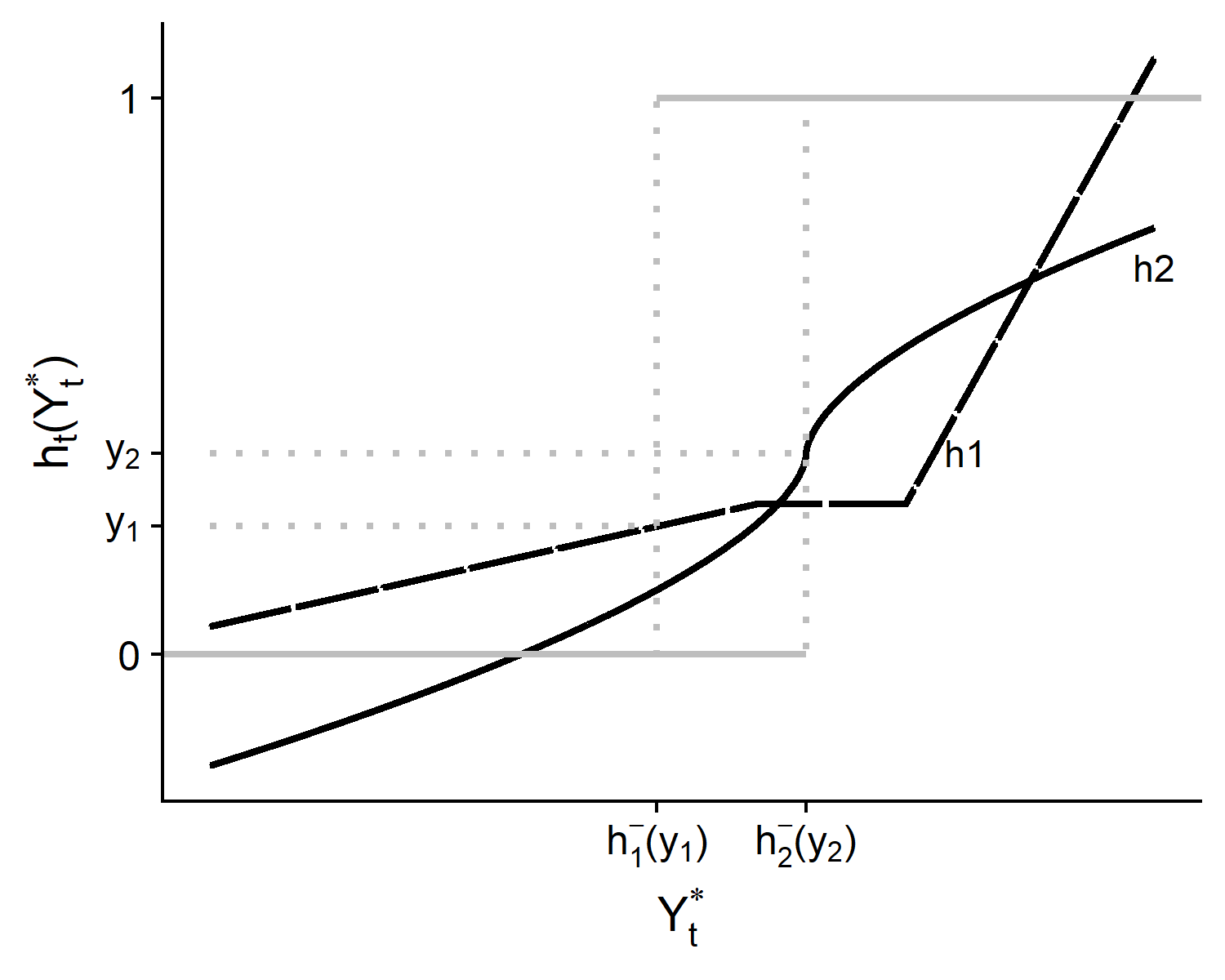
Figure 3.1: FELT functions $h_{1}$ and $h_{2}$.

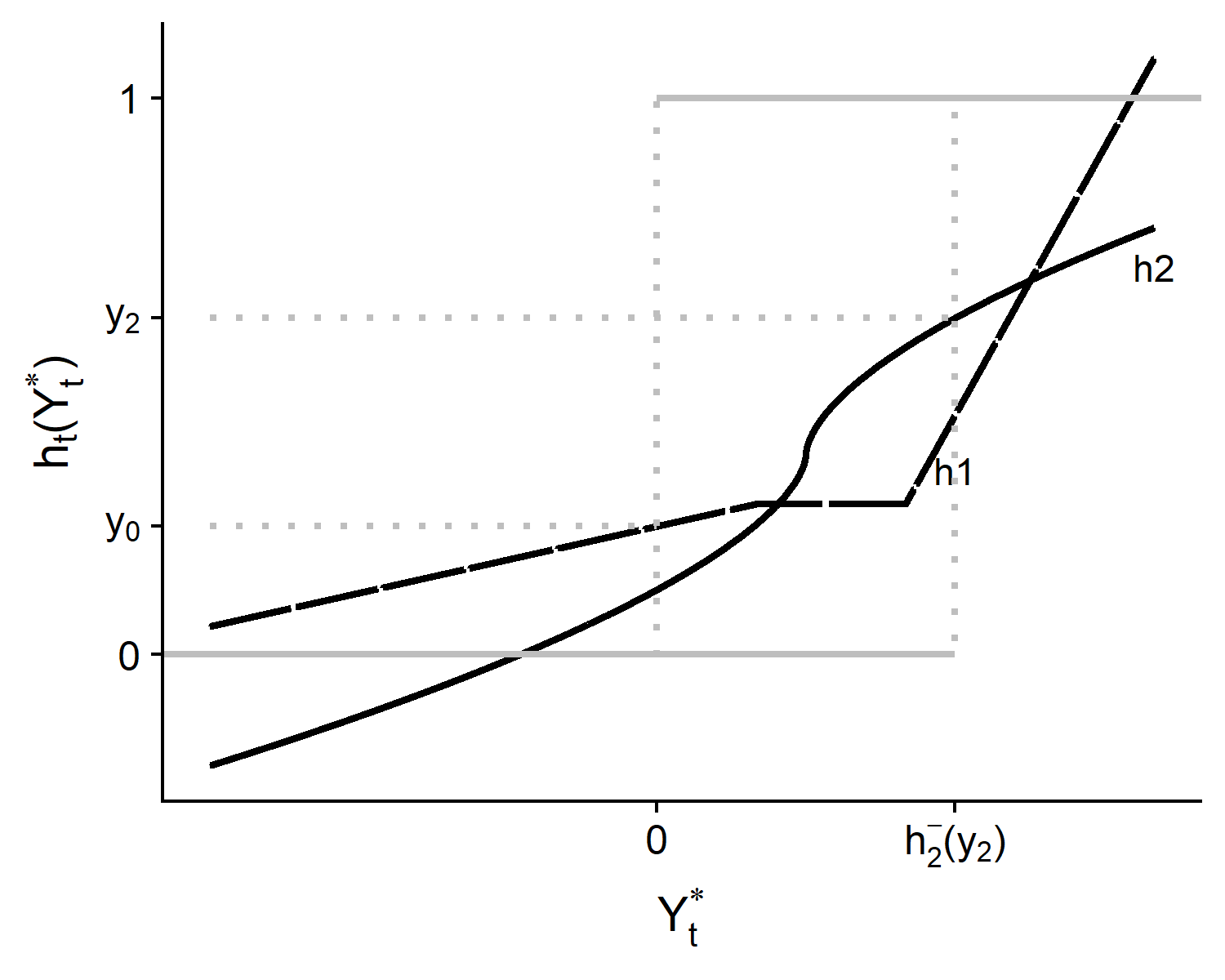
Figure 3.2: Normalization and tracing.

3.2 Nonparametric errors

In this section, we provide nonparametric identification results for $\left(\beta,h_{1},h_{2}\right)$. Parts of our identification proof build on Manski, (1987), who in turn builds on Manski, (1975, 1985).

Assumption 2.

[Error terms]

(i) $F_{1}(u|\alpha,X)=F_{2}(u|\alpha,X)\equiv F(u|\alpha,X)$ for all $(\alpha,X)$;

(ii) The support of $F(\left.u\right|\alpha,X)$ is $\mathbb{R}$ for all $\left(\alpha,X\right)$.

Assumption 2 places no parametric distributional restrictions on the distribution of $U_{it}$ and allows the stochastic errors $U_{it}$ to be correlated across time. The first part of the assumption, 2(i), is a stationarity assumption, requiring time-invariance of the distribution of the error terms conditional on the trajectory of the observed regressors and on the unobserved heterogeneity. This assumption excludes lagged dependent variables as covariates. Additionally, as noted by, e.g., Chamberlain, (2010), although it allows for heteroskedasticity, it restricts the relationship between the observed regressors and $U_{it}$ by requiring that even when $x_{1}\not=x_{2}$, $U_{1}$ and $U_{2}$ have equal skedasticities. This type of stationarity assumption is common in linear and nonlinear panel models, e.g., Chernozhukov et al., (2013) and references therein.

Assumption 2(ii) requires full support of the error terms. It guarantees that, for any pair $\left(y_{1},y_{2}\right)\in\underline{\mathcal{Y}}^{2}$, the probability of being a switcher is positive. In our context, being a switcher refers to the event $D_{1}\left(y_{1}\right)+D_{2}\left(y_{2}\right)=1$, so that Assumption 2 guarantees that $P\left(D_{1}\left(y_{1}\right)+D_{2}\left(y_{2}\right)=1\right)>0$. This assumption is similar to Assumption 1 in Manski, (1987).

Let $\Delta X\equiv X_{2}-X_{1}\,$ and for an arbitrary pair $(y_{1},y_{2})\in\mathcal{\underline{Y}}^{2},$ define

$$\gamma\left(y_{1},y_{2}\right) \equiv h_{2}^{-}\left(y_{2}\right)-h_{1}^{-}\left(y_{1}\right).$$ (3.3)

Lemma 1.

Suppose that $\left(Y,X\right)$ follows the model in (3.1). Let Assumptions 1 and 2 hold. Then for all $\left(y_{1},y_{2}\right)\in\underline{\mathcal{Y}}^{2},$

$$\operatorname{med}\left(D_{2}\left(y_{2}\right)-D_{1}\left(y_{1}\right)|X,\,D_{1}\left(y_{1}\right)+D_{2}\left(y_{2}\right)=1\right)=\operatorname{sgn}\left(\Delta X\beta-\gamma\left(y_{1},y_{2}\right)\right).$$ (3.4)

Proof.

The proof builds on Manski, (1985, 1987), and is presented in Appendix A.1. ∎

Let $W\equiv(\Delta X,-1)^{\prime}$ and $\theta\left(y_{1},y_{2}\right)\equiv\left(\beta,\gamma\left(y_{1},y_{2}\right)\right),$ so that $\left(\ref{eq:med_sgn}\right)$ can be written as

$$\text{med}\left(D_{2}\left(y_{2}\right)-D_{1}\left(y_{1}\right)|X,D_{1}\left(y_{1}\right)+D_{2}\left(y_{2}\right)=1\right)=\text{sgn}\left(W\theta\left(y_{1},y_{2}\right)\right).$$

For identification of $\theta\left(y_{1},y_{2}\right)$ we impose the following additional assumptions.

Assumption 3.

[Covariates]

(i) The distribution of $\Delta X$ is such that at least one component of $\Delta X$ has positive Lebesgue density on $\mathbb{R}$ conditional on all the other components of $\Delta X$ with probability one. The corresponding component of $\beta$ is non-zero.

(ii) The support of $W$ is not contained in any proper linear subspace of $\mathbb{R}^{K+1}$.

Assumption 3(i) requires that the change in one of the regressors be continuously distributed conditional on the other components. Assumption 3(ii) is a full rank assumption. These assumptions are standard in the binary choice literature concerned with point identification of the parameters.

Assumption 3 resembles Assumption 2 in Manski, (1987), the difference being that our assumption concerns $W$, which includes a constant that captures a time trend. The presence of this constant requires sufficient variation in $X_{t}$ over time. No linear combination of the components of $X_{t}$ can equal the time trend.

Assumption 4.

[Normalization-$\beta$] For any $(y_{1},y_{2})\in\mathcal{\underline{Y}}^{2},$ $\theta\left(y_{1},y_{2}\right)\in\Theta=\mathcal{B}\times\mathbb{R},$ where $\mathcal{B}=\left\{\beta:\beta\in\mathbb{R}^{K},\|\beta\|=1\right\}$.

Assumption 4 imposes a normalization on $\beta$, namely that the norm of the regression coefficient equals 1. Scale normalizations are standard in the binary choice literature, and are necessary for point identification when the distribution of the error terms is not parameterized. Normalizing $\beta$ (instead of $\theta$) avoids a normalization that would otherwise depend on the choice of $\left(y_{1},y_{2}\right)$. In this way, the scale of $\beta$ remains constant across different choices of $\left(y_{1},y_{2}\right)$. Alternatively, one can normalize the coefficient on the continuous covariate (cf. Assumption 3(i)) to be equal to one. In our economic model in Section 5 the latter assumption holds automatically.

Theorem 1.

Suppose that $\left(Y,X\right)$ follows the model in (3.1), and let the distribution of $\left(Y,X\right)$ be observed. Let Assumptions 1, 2, 3, and 4 hold. Then, for an arbitrary pair $\left(y_{1},y_{2}\right)\in\underline{\mathcal{Y}}^{2},$ $\theta\left(y_{1},y_{2}\right)$ is identified.

Proof.

The proof proceeds by showing that FELT can be converted into a binary choice model for an arbitrary pair $\left(y_{1},y_{2}\right),$ and then builds on Theorem 1 in Manski, (1987), which in turn uses results in Manski, (1985). See Appendix A.2. ∎

So far, we have identified the regression coefficient $\beta$ and the difference in the generalized inverses at arbitrary pairs $\left(y_{1},\,y_{2}\right)$. We consider now identification of the functions $h_{1}$ and $h_{2}$ on $\underline{\mathcal{Y}}$.

Assumption 5.

[Normalization-$h_{1}$] For some $y_{0}\in\mathcal{\underline{\mathcal{Y}}},$ $h_{1}^{-}\left(y_{0}\right)=0$.

Such a normalization is standard in transformation models, see, e.g., Horowitz, (1996). Without this normalization, all identification results hold up to $h_{1}^{-}\left(y_{0}\right)$. We normalize the function in the first time period only, imposing no restrictions on the function in the second period beyond that of weak monotonicity (cf. Assumption 1). In Section 4, we show that this normalization assumption is not necessary for our results on the identification of the conditional mean or of the conditional variance of the fixed effects.

Theorem 2.

Suppose that $\left(Y,X\right)$ follows the model in (3.1), and let the distribution of $\left(Y,X\right)$ be observed. Under Assumptions 1, 2, 3, 4, and 5, the transformations $h_{1}$ and $h_{2}$ are identified.

Proof.

The proof proceeds by identifying the generalized inverses of monotone functions, which obtains identification of the pre-images of $h_{1}$ and $h_{2}$. This obtains identification of the functions themselves. See Appendix A.3. ∎

3.3 Logit errors

In this section, we show identification of $\left(\beta,h_{1},h_{2}\right)$ when the error terms are assumed to follow the standard logistic distribution. The logistic case is not nested in the nonparametric case. In particular, when the errors are logistic, we do not require a continuous regressor. However, we require conditional serial independence of the error terms.

Assumption 6.

[Logit] (i) $F_{1}(u|\alpha,X)=F_{2}$$\left(u|\alpha,X\right)=\Lambda\left(u\right)=\frac{\exp\left(u\right)}{1+\exp\left(u\right)}$, and $U_{1}$ and $U_{2}$ are independent; (ii) $E(W^{\prime}W)$ is invertible.

Assumption 6(i) strengthens Assumption 2 by requiring the errors to follow the standard logistic distribution and to be serially independent. Note that one consequence of this assumption, which specifies the variance of the error terms to be equal to 1, is to eliminate the need to normalize $\beta$. On the other hand, Assumption 6(ii) imposes weaker restrictions on the observed covariates relative to Assumption 3, since it does not require the existence of a continuous covariate. Sufficient variation in $\Delta X$ is sufficient to obtain identification of the vector $\beta$ when the error terms follow the standard logistic distribution.

Theorem 3.

Suppose that $\left(Y,X\right)$ follow the model in (3.1), and let the distribution of $\left(Y,X\right)$ be observed. Let Assumptions 1 and 6 hold. Then, for an arbitrary pair $\left(y_{1},y_{2}\right)\in\mathcal{\underline{Y}}^{2},$ $\theta\left(y_{1},y_{2}\right)$ is identified. Additionally, letting Assumption 5 hold, then the transformations $h_{1}\left(\cdot\right)$ and $h_{2}\left(\cdot\right)$ are identified.

Proof.

See Appendix A.4. ∎

4 Conditional distribution of fixed effects

If $(h_{1},h_{2})$ are invertible, we can use the previous identification theorem to identify features of the distribution of the fixed effects conditional on observed regressors. These features are the change in the conditional mean function of $\alpha$ and the conditional variance of $\alpha$ conditional on $X_{1},X_{2}$. These results are relevant since in our collective household model, the fixed effects represent the log of resource shares, and both the standard deviation of these resource shares and the response of their conditional mean to covariates are key parameters of interest in the empirical literature. As this is relevant to our application, we note here that a normalization assumption, such as 4, on the demand function in the first period is not necessary for these results on the resource shares because, e.g., we only need their deviation with respect to the mean of the fixed effects.

In this section, we provide sufficient conditions for the identification of the change in the conditional mean function of the fixed effects, defined as:

$$\mu\left(x\right)\equiv E\left[\left.\alpha\right|X=x\right],\text{ for all $x\in\mathcal{X},$}$$ (4.1)

as well as for the conditional variance of the fixed effects. For these results, the normalization assumption 5 is not necessary. To provide intuition for this, let

$$c_{1}\equiv h_{1}^{-1}\left(y_{0}\right),$$

at an arbitrary $y_{0}\in\mathcal{\underline{Y}}$ and $g_{t}\left(y\right)\equiv h_{t}^{-1}\left(y\right)-c_{1}$ for all $y\in\mathcal{\underline{Y}}$. Note that Theorem 1 recovers

$$\widetilde{U}_{t}\equiv\alpha-U_{t}=h_{t}^{-1}\left(Y_{t}\right)-X_{t}\beta,$$

up to $c_{1}$, so that the joint distribution of $\left(\widetilde{U}_{1},\widetilde{U}_{2},X_{1},X_{2}\right)$ is identified up to $c_{1}$. By placing restrictions on the distribution of $\left(\alpha,U_{1},U_{2},X_{1},X_{2}\right)$, we can then recover our features of interest.

Theorem 4.

(i) Let the assumptions of Theorem 1 hold, and additionally assume that (4a) $\left(h_{1},h_{2}\right)$ are strictly increasing, and (4b) let $m\in\mathbb{R}$ be an unknown constant such that $E\left(\left.U_{t}\right|X=x\right)=m$, for all $x\in\mathcal{X}$. Then, for any $x,x^{\prime}\in\mathcal{X}$, the change in the conditional mean function $\mu\left(x\right)-\mu\left(x^{\prime}\right)$ is identified and given by

$$\mu\left(x\right)-\mu\left(x^{{}^{\prime}}\right)=E\left[\left.g_{t}\left(Y_{t}\right)-X_{t}\beta\right|X=x\right]-E\left[\left.g_{t}\left(Y_{t}\right)-X_{t}\beta\right|X=x^{{}^{\prime}}\right].$$

Proof.

See Appendix A.5. ∎

Remark 1.

As opposed to our main identification result in Theorem 2, Theorem 4 does not use a normalization on the functions $\left(h_{1},h_{2}\right)$. If we were to impose the normalization in Assumption 5, the conditional mean function $\mu\left(x\right)$ would be identified for all $x\in\mathcal{X}$. This result provides justification for nonparametric regression of $\alpha$ on observables (up to location).

Remark 2.

Under slightly weaker conditions, we can obtain the projection coefficients of $\alpha$ on $X_{t}$. This is of interest for our empirical application. Recall that the joint distribution of $\left(\widetilde{U}_{1},\widetilde{U}_{2},X_{1},X_{2}\right)$ is identified up to $c_{1}$. Then, assuming $\text{Cov}\left(U_{s},X_{t}\right)=0$, we can identify the projection coefficient of $\alpha$ on $X_{t}$ from

$$\left[\text{Var}\left(X_{t}\right)\right]^{-1}\text{Cov}\left(\alpha,X_{t}\right)=\left[\text{Var}\left(X_{t}\right)\right]^{-1}\text{Cov}\left(\alpha-U_{s},X_{t}\right)=\left[\text{Var}\left(X_{t}\right)\right]^{-1}\text{Cov}\left(\widetilde{U}_{s},X_{t}\right).$$

Second, define the conditional variance of the fixed effects as

$$\sigma_{\alpha}^{2}\left(x\right)\equiv Var\left[\left.\alpha\right|X=x\right],\text{ for all $x\in\mathcal{X}.$}$$ (4.2)

For this second result, we strengthen our assumptions to include, among others, serial independence of the error term. This allows us to pin the persistence in unit $i$’s time series on $\alpha_{i}$ instead of on serial dependence in the errors.

Theorem 5.

Let the assumptions of Theorem 1 hold and assume that (5a) $\left(h_{1},h_{2}\right)$ are strictly increasing, and (5b) $Cov\left[\left.\alpha,U_{t}\right|X=x\right]=0$ for all $x\in\mathcal{X}$ and $t$, and (5c) $Cov\left[\left.U_{1},U_{2}\right|X=x\right]=0$ for all $x\in\mathcal{X}$. Then for all $x\in\mathcal{X},$ the conditional variance function $\sigma_{\alpha}^{2}\left(x\right)$ is identified and given by:

$$\sigma_{\alpha}^{2}\left(x\right)=Cov\left(\left.g_{2}\left(Y_{2}\right)-X_{2}\beta,g_{1}\left(Y_{1}\right)-X_{1}\beta\right|X=x\right).$$

Proof.

See Appendix A.5. ∎

It may be possible to obtain the entire conditional distribution of the fixed effects under the assumption that $\left(\alpha,U_{1},U_{2}\right)$ are mutually independent by using arguments similar to those in Arellano and Bonhomme, (2012).

5 Microeconomic model

In this section, we construct a model of an efficient full-commitment intertemporal collective (FIC) household. We provide sufficient conditions implying that observed household-level quantity demand equations are time-varying functions of fixed effects that lie in the FELT class.

Essentially, we adapt the intertemporal collective household model of Chiappori and Mazzoco, (2017) to the model of household scale economies given in the static household model of Browning et al., (2013). We assume efficiency, i.e. that the household members together reach the Pareto frontier. Consequently, our model does not account for inefficiency due to e.g. consumption externalities or information asymmetries.

We use subscripts $i,j,t$. Let $i=1,...,n$ index households and assume the household has a time-invariant composition, with $N_{ij}$ members of type $j$. Let $j=m,f,c$ for men, women and children. Let $t=1,2$. Let $z$ be a vector of time-varying household-level demographic characteristics, and let the numbers of household members of each type, $N_{im}$, $N_{if}$ and $N_{ic}$, be (time-invariant) elements of $z_{it}$. Like Chiappori and Mazzoco, (2017), this is a model with uncertainty, so we use the superscript $s=1,2$ to index states in the second period only. As in Chiappori and Mazzoco, (2017), the use of 2 time periods and 2 states is for illustration only; the model goes through with any finite number of states or periods. Similarly, inclusion of a risky asset would not change the features of the model that we use.

Indirect utility, $V_{j}(p,x,z)$, is the maximized value of utility given a budget constraint defined by prices $p$ and budget $x$, given characteristics $z$. Let $V_{j}$ be strictly concave in the budget $x$. Indirect utility depends on time only through its dependence on the budget constraint and time-varying demographics $z$. Let $v_{ijt}\equiv V_{j}(p_{t},x_{it},z_{it})$ denote the utility level of a person of type $j$ in household $i$ in period $t$.

Household decisions are made on the basis of individual shadow budget constraints, reflecting the economic environment within the household. These shadow constraints are characterized by a shadow price vector faced by all members and shadow budgets which may differ across household members. Let $A_{it}\equiv A(z_{it})$ be a diagonal matrix that gives the shareability of each good, and let it depend on demographics $z_{it}$ (including the numbers of household members). More shareable goods have lower shadow prices of within-household consumption.

For nonshareable goods, the corresponding element of $A_{it}$ equals $1$; for shareable goods, it is less than $1$, possibly as small as $1/N_{i}$ where $N_{i}$ is the number of household members. Goods may be partly shareable, with an element of $A_{it}$ between $1/N_{i}$ and $1$. With market prices $p_{t}$, within-household shadow prices are given by the linear transformation $A_{it}p_{t}$.

Browning et al., (2013) also allow for inequality in shadow budgets. Let $\eta_{ijt}$ be the resource share of type $j$ in household $i$ in time period $t$. It gives the fraction of the household budget consumed by that type. Each person of the $N_{ij}$ people of type $j$ consumes $\eta_{ijt}/N_{ij}$ of the household budget $x_{it}$, so they each have a shadow budget of $\eta_{ijt}x_{it}/N_{ij}$.

Each household member faces a shadow budget of $\eta_{ijt}x_{it}/N_{ij}$ and shadow prices of $A_{it}p$_t, so that, within the household, indirect utility is given by

$$v_{ijt}=V_{j}\left(A_{it}p_{t},\eta_{ijt}x_{it}/N_{ij},z_{it}\right).$$ (5.1)

Let $V_{xj}(p,w,z)\equiv\partial V_{j}(p,w,z)/\partial w$ be the monotonically decreasing marginal utility of person $j$ with respect to their shadow budget. Then, $V_{xj}\left(A_{it}p_{t},\eta_{ijt}x_{it}/N_{ij},z_{it}\right)$ is the value of their marginal utility evaluated at their shadow budget constraint.

Let $p_{2}^{s},z_{i2}^{s},\overline{x}_{i}^{s}$ for $s=1,2$ be the possible realizations of state-dependent variables that occur with household-specific probabilities $\pi_{i}^{1}$ and $\pi_{i}^{2}$ (which sum to $1$). Here, $\overline{x}_{i}^{s}$ is the state-specific lifetime wealth of household $i$, revealed in period $2$.

Pareto weights $\phi_{ij}$ vary arbitrarily across households, and depend, for example, on the household-specific expectation of lifetime wealth at the moment of household formation. Because ours is a full commitment model, Pareto weights do not have a time subscript because they are fixed at the moment of household formation, when the full-commitment contract is set. This household-level time-invariant variable will form the basis of our fixed-effects variation.

As in Chiappori and Mazzoco, (2017),the assumption of efficiency implies that we can represent the household’s decisions via the Bergson-Samuelson Welfare Function, $W_{i}$, for the household is

$$W_{i}\equiv\sum_{j=1}^{J}N_{ij}\phi_{ij}\left[v_{ij1}+\sum_{s=1}^{2}\rho_{i}\pi_{i}^{s}v_{ij2}^{s}\right].$$ (5.2)

The term in square brackets is the expected lifetime utility, discounted by the discount factor $\rho_{i}$, of each member of type $j$ in household $i$. Each member of type $j$ gets the Pareto weight $\phi_{ij}$. The assumption of efficiency implies that the household reaches the Pareto Frontier; the Pareto weights pinpoint which point on the Frontier is chosen by the household.

Next, substitute indirect utility (5.1) for utility $v_{ij1}$ and $v_{ij2}^{s}$ into (5.2), and form the Lagrangian using the intertemporal budget constraint with interest rate $\tau$, $x_{i1}+x_{i2}^{s}/(1+\tau)=\overline{x}_{i}^{s}$, and the adding-up constraints on resource shares, $\sum_{j}\eta_{ij1}=\sum_{j}\eta_{ij2}^{s}=1.$ Each household $i$ chooses $x_{i1},$ $\eta_{ij1}$ and $\eta_{ij2}^{s}$ to maximize $W_{i}$. Solving this optimization problem obtains for any two types, $j$ and $k$, that:

$$\frac{\phi_{ij}}{\phi_{ik}}=\frac{V_{xk}(A_{i1}p_{1},\eta_{ik1}x_{i1}/N_{ik},z_{i1})}{V_{xj}(A_{i1}p_{1},\eta_{ij1}x_{i1}/N_{ij},z_{i1})}=\frac{V_{xk}(A_{i2}p_{2}^{s},\eta_{ik2}^{s}x_{i2}^{s}/N_{ik},z_{i2}^{s})}{V_{xj}(A_{i2}p_{2}^{s},\eta_{ij2}^{s}x_{i2}^{s}/N_{ij},z_{i2}^{s})},$$ (5.3)

for $s=1,2$ for all $i$. That is, the household chooses resource shares so as to equate ratios of marginal utilities with ratios of Pareto weights.

An assignable good is one where we observe the consumption of that good by a specific person (or type of person). Assuming the existence of a scalar-value demand function $q_{j}(p,x,z)$ for an assignable and non-shareable good (e.g., food or clothing) for a person of type $j$, Browning et al., (2013) show that the household’s quantity demand, $Q_{ijt}$, for the assignable good for each of the $N_{ij}$ people of type $j$ is given by

$$Q_{ijt}=q_{j}(A_{it}p_{t},\eta_{ijt}x_{it}/N_{ij},z_{it}).$$

Assuming that the assignable good is a normal good implies that $q_{j}$ is strictly increasing in its second argument, and is therefore strictly monotonic.

Since $p_{t}$ is unobserved and varies over time, we can express $Q_{ijt}$ as a time-varying function of observed data. Defining $\widetilde{q}_{jt}(x,z)=q_{j}(p_{t},x,z)$, we have

$$Q_{ijt}=\widetilde{q}_{jt}(\eta_{ijt}x_{it}/N_{ij},z_{it}).$$ (5.4)

This is the structural demand equation that we ultimately bring to the data.

The model above determines resource share via the first-order conditions (5.3), and these resource shares depend on time-invariant Pareto weights $\phi_{ij}$. But these resource shares are a vector of implicit functions, which may be hard to work with. To make the model tractable, we impose sufficient structure on utility functions to find closed forms for resource shares.

In our empirical example below, we work with data that have time-invariant demographic characteristics, so let $z_{it}=z_{i}$ be fixed over time. This implies that the shareability of goods embodied in $A$ is time-invariant: $A_{it}=A_{i}=A(z_{i})$. We will estimate the demand equation for women’s food in nuclear households comprised of $1$ man, $1$ woman and $1-4$ children, so $N_{if}=N_{im}=1$.

Let indirect utilities be in the price-independent generalized logarithmic (PIGL) class (Muellbauer, (1975, 1976)) given by

$$V_{j}(p,x,z)=C_{j}(p,z)+\left(B(p,z)x\right)^{r(z)}/r(z).$$ (5.5)

Here, $V_{j}$ is homogeneous of degree $1$ in $p,x$ if $C_{j}$ is homogeneous of degree $0$ in $p$ and $B$ is homogeneous of degree $-1$ in $p$. $V$ is increasing in $x$ if $B(p,z)$ is positive and $V$ is concave in $x$ if $r(z)<1$. In terms of preferences, this class is reasonably wide. It gives quasihomothetic preferences if $r(z)=1$, and PIGLOG preferences as $r(z)\rightarrow 0$ (this includes the Almost Ideal Demand System of Deaton and Muellbauer, (1980)).

The functions $C_{j}$ vary across types $j$, and so the model allows for preference heterogeneity between types, e.g., between men and women. The restrictions that $B(p,z)$ and $r(z)$ don’t vary across $j$ and that $r(z)$ does not depend on prices $p$ are important: as we see below, they imply that resource shares are constant over time.

Substituting into the BCL model, observed demographics and period $t$ budgets, we have that marginal utilities are given by

$$V_{xj}(A_{it}p_{t},\eta_{ijt}x_{it}/N_{ij},z_{it})=B(A_{i}p_{t},z_{i})^{r(z_{i})}\left(\eta_{ijt}x_{it}/N_{ij}\right)^{r(z_{i})-1}.$$

For $r(z_{i})\neq 1$, and for any pair of types $j,k\text{, }$we substitute into (5.3) and rearrange to get

$$\left(\frac{\eta_{ikt}}{\eta_{ijt}}\right)=\frac{N_{ik}}{N_{ij}}\left(\frac{\phi_{ij}}{\phi_{ik}}\right)^{1/\left(r(z_{i})-1\right)}.$$ (5.6)

The household chooses resource shares in each period and each state to satisfy (5.6). Since the right-hand side has no variation over time or state, this implies that, given PIGL utilities (5.5), the resource shares in a given household $i$ are independent of period $t$ and state $s$. However, resource shares do vary with both observed and unobserved variables across households $i$.

Let the fixed resource shares that solve the first-order conditions with PIGL demands be denoted $\overline{\eta}_{ij}$, and define

$$\alpha_{i}\equiv\ln\left(\overline{\eta}_{if}/N_{if}\right)=\ln\overline{\eta}_{if},$$ (5.7)

to equal to the logged resource share of the woman in the household.

Let there be a multiplicative Berkson, (1950) measurement error denoted $\exp\left(-U\right)$ which multiplies the budget, so that if we observe $x$, the actual budget is $x/\exp\left(U\right)$. The measurement error is i.i.d. across time and households, which implies stationarity of $U$. Here, the measurement error does not affect resource shares, but does affect the distribution of observed quantity demands. Then household demand for women’s food (the assignable good), $Q_{ift}$, is given by

$$Q_{ift}=\widetilde{q}_{ft}(\exp\left(\alpha_{i}\right)x_{it}/\exp\left(U_{it}\right),z_{i}).$$

This is a FELT model, conditional on covariates:

$$Y_{it}=h_{t}(Y_{it}^{*},z_{i}),$$ (5.8)

where $h_{t}(Y_{it}^{*},z_{i})=\widetilde{q}_{ft}\left(\exp\left(Y_{it}^{*}\right),z_{i}\right)$, $Y_{it}^{*}=\alpha_{i}+X_{it}-U_{it}$, and $X_{it}=\ln x_{it}$ is the logged household budget.

The assumption that the assignable good is normal means that the time-varying functions $h_{t}$ are strictly monotonic in $Y_{it}^{*}$. One could additionally impose that the demand functions $\widetilde{q}_{ft}$ come from the application of Roy’s Identity to the indirect utility function (5.5). These demand functions equal a coefficient times the shadow budget plus a coefficient times the shadow budget raised to a power, where the coefficients are time-varying and depend on $z_{i}$. We do not impose that additional structure here; instead, we show in Section 7 that the estimated demand curves given by FELT are close to the PIGL shape restrictions.

Here, the time-dependence of $h_{t}$ is economically important; it is driven by the price-dependence of preferences and by the fact that prices are common to all households $i$ but vary over time $t$. Further, the fixed effects $\alpha_{i}$ are economically meaningful parameters: they are equal to the logged women’s resource shares in each household. The standard deviation of the logs is a common inequality measure, and the standard deviation of $\alpha_{i}$ is identified by FELT given strict monotonicity, as we show in Section 4. Further, the covariation of $\alpha_{i}$ with observed regressors is identified.

6 Data

We use data from the $2012$ and $2015$ Bangladesh Integrated Household Surveys. This data set is a household survey panel conducted jointly by the International Food Policy Research Institute and the World Bank. In this survey, a detailed questionnaire was administered to a sample of rural Bangladeshi households. This data set has two useful features for our purposes: 1) it includes person-level data on food intakes and household-level data on total household expenditures; and 2) it is a panel, following roughly $6000$ households over two (nonconsecutive) years. The former allows us to use food as the assignable good to identify our collective household model parameters. The latter allows us to model household-level unobserved heterogeneity in women’s resource shares.

The questionnaire was initially administered to $6503$ households in $2012$, drawn from a representative sample frame of all rural Bangladeshi households. Of these, $6436$ households remained in the sample in $2015$. In these data, expenditures on food include imputed expenditure from home production. We drop households with a discrepancy between people reported present in the household and the personal food consumption record, and households with no daily food diary data. Of the remaining data, $6205$ households have total expenditures reported for both $2012$ and $2015$.

In this paper, we focus on households that do not change members between periods. There are $1920$ households whose composition is unchanged between $2012$ and $2015$. Roughly half of these households have more than one adult man or more than one adult women. To simplify the interpretation of estimated resource shares we focus on nuclear households. This leaves $871$ nuclear households comprised of one man, one woman and $1$ to $4$ children, where children are defined to be $14$ years old or younger.

Our household-level annual expenditure, $x_{it},$ is the sum of total expenditure on, and imputed home-produced consumption of, the following categories of consumption: rent, food, clothing, footwear, bedding, non-rent housing expense, medical expenses, education, remittances, religious food and other offerings (jakat/ fitra/ daan/ sodka/ kurbani/ milad/ other), entertainment, fines and legal expenses, utensils, furniture, personal items, lights, fuel and lighting energy, personal care, cleaning, transport and telecommunication, use-value from assets, and other miscellaneous items. These spending levels derive from one-month and three-month duration recall data in the questionnaire, and are grossed up to the annual level. Estimation uses $X_{it}=\ln x_{it}$, the natural logarithm of annual consumption.

The assignable good, $Y_{it}$, is annual expenditure on food for the woman. The surveys contains a one-day (24-hour) food diary with data on person-level quantities (measured in kilograms) of food consumption in 7 categories: Cereals, Pulses, Oils; Vegetables; Fruits; Proteins; Drinks and Others. These consumption quantities include home-produced food and purchased food and gifts. They include both food consumed in the home (both cooked at home and prepared ready-to-eat food), as well as food consumed outside the home (at food carts or restaurants). These one-day food quantities are transformed into one-day food expenditures by multiplying by estimated village-level unit-values (following Deaton, (1997)), and from this, the woman’s share of one-day household food expenditure is calculated. Finally, the woman’s annual expenditure on food is calculated as her share of one-day food expenditure multiplied by the household’s total annual food expenditure (from recall data).

Our model is also conditioned on a set of time-invariant demographic variables $z_{i}$. We include several types of observed covariates in $z_{i}$ that may affect both preferences and resource shares: 1) the age in $2012$ of the adult male; 2) the age in $2012$ of the adult female; 3) the average age in $2012$ of the children; 4) the average education in years of the adult male; 5) the average education in years of the adult female; 6) an indicator that the household has 2 children; 7) an indicator that the household has 3 or 4 children; and 8) the fraction of children that are girls.

For the first five of these demographic variables, in order to reduce the support of the regressors, we top- and bottom-code each variable so that values above (below) the $95^{th}$ ($5^{th}$) percentiles equal the $95^{th}$ ($5^{th}$) percentile values. For all seven of these variables, we standardize the location and scale so that their support is $[0,1]$. This support restriction simplifies our monotonicity restrictions when it comes to estimation, as explained in Section 7.

We do not trim the data for outliers in the budget or food quantity demands. Instead, we trim the support of the estimated nonparametric regression functions to account for fact that these estimators are high-variance near their boundaries.

Table $2$ in the Appendix, Section C gives summary statistics on these data.

7 Estimation of Resource Shares

Following our identification results, estimation could be based on composite versions of the maximum score estimator or the conditional logit estimator (see Botosaru and Muris, (2017)). Here, we instead follow a sieve GMM approach that facilitates the inclusion of a large vector of demographic conditioning variables $z$ and the imposition of strict monotonicity on the demand functions (aka: normality of the assignable good).

The women’s food demand equation (5.8) is a FELT model, conditional on observed covariates $z$. Denote the inverse demand functions $g_{t}(Y_{it},z_{it})=h_{t}^{-1}(\cdot,z_{it})$. Given (5.8) a two-period setting with $t=1,2$, and time-invariant demographics $z_{it}=z_{i}$, we have

$$\alpha_{i}+X_{it}-U_{it}=g_{t}(Y_{it},z_{i}),$$ (7.1)

implying the conditional moment condition

$$E\left[\left.g_{2}(Y_{i2},z_{i})-g_{1}(Y_{i1},z_{i})-\triangle X_{it}\right|X_{i1},X_{i2},z_{i}\right]=0,$$ (7.2)

using stationarity of the conditional distribution of the Berkson errors $\exp\left(-U_{it}\right)$.

We provide a detailed description of our GMM estimator in Appendix B. Briefly, we approximate the inverse demand functions, $g_{t}$, $t=1,2,\text{ }$ using 8th order Bernstein polynomials to impose monotonicity (estimates for other orders are reported in Appendix D) and use the nonparametric bootstrap for inference. Because the nonparametric bootstrap may not be valid for this case, we take our estimated confidence intervals with caution, see Appendix B.

We characterize several interesting features of the distribution of resource shares. Recall from Theorems 4 and 5 that identification of features of this distribution does not impose a normalization on assignable good demand functions, and only identifies the distribution of logged resource shares (fixed effects) up to location. Consequently, we only identify features of the resource share distribution up to a scale normalization. This is related to identification results in Chiappori and Ekeland, (2009) which show identification up to location using assignable goods.

Let $\widehat{g}_{it}=\widehat{g}_{t}(Y_{it},z_{i})$ equal the predicted values of the inverse demand functions at the observed data. Recall that $g_{t}\left(Y_{it},z_{i}\right)=\alpha_{i}+X_{it}-U_{it},$ so we can think of $\widehat{g}_{it}-X_{it}$ as a prediction of $\alpha_{i}-U_{it}$. We then compute the following summary statistics of interest, leaving the dependence of $\hat{g}_{it},\,t=1,2,$ on $z_{i}$ implicit:

1. an estimate of the standard deviation of $\alpha_{i}$ given by

   $$\hat{std}\left(\alpha\right)=\sqrt{\hat{cov}\left(\left(\widehat{g}_{i2}-X_{i2}\right),\left(\widehat{g}_{i1}-X_{i1}\right)\right)},$$

   where $\hat{cov}$ denotes the sample covariance. The standard deviation of logs is a standard (scale-free) inequality measure. So this gives a direct measure of inter-household variation in women’s resource shares.

2. an estimate of the standard deviation of the projection error, $e_{i},$ of $\alpha_{i}$ on $\bar{X}_{i}=\frac{1}{2}\left(X_{i1}+X_{i2}\right)$ and $Z_{i}$. Consider the projection

   $$\alpha_{i}=\gamma_{1}\bar{X}_{i}+\gamma_{2}Z_{i}+e_{i},$$

   where $Z_{i}$ contains a constant. We are interested in the standard deviation of $e_{i}$. To obtain this parameter, we compute estimators for $\gamma_{1},\gamma_{2}$ from the pooled linear regression of $\hat{g}_{it}-X_{it}$ on $\bar{X}_{i}\text{ and }Z_{i}.$ Call these estimators $\hat{\gamma}_{1},\hat{\gamma}_{2}$. Then, as in $\hat{std}\left(\alpha\right)$ in (1), an estimate of the standard deviation of $e_{i}$ is given by:

   $$\hat{std}\left(e_{i}\right)=\sqrt{\hat{cov}\left(\left(\widehat{g}_{i2}-X_{i2}-\hat{\gamma}_{1}\bar{X}_{i}-\hat{\gamma}_{2}Z_{i}\right),\left(\widehat{g}_{i1}-X_{i1}-\hat{\gamma}_{1}\bar{X}_{i}-\hat{\gamma}_{2}Z_{i}\right)\right)}.$$

   This object measures the amount of variation in $\alpha_{i}$ that cannot be explained with observed regressors. If it is zero, then we don’t really need to account for household-level unobserved heterogeneity in resource shares. It is much larger than zero, then accounting for household-level unobserved heterogeneity is important.

3. an estimate of the standard deviation of $\alpha_{i}+X_{it}$ for $t=1,2$, computed as

   $$\hat{std}\left(\alpha_{i}+X_{it}\right) =\sqrt{\hat{var}\left(\alpha_{i}\right)+\hat{var}\left(X_{it}\right)+2\hat{cov}\left(\alpha_{i},X_{it}\right)},$$

   where

   $$\hat{cov}\left(\alpha_{i},X_{i1}\right) =cov\left(\hat{g}_{i1}-X_{i1},X_{i1}\right),$$

   $$\hat{cov}\left(\alpha_{i},X_{i2}\right) =cov\left(\hat{g}_{i2}-X_{i2},X_{i2}\right),$$

   and $\hat{var}\left(\alpha_{i}\right)=\left(\hat{std}\left(\alpha\right)\right)^{2}$ and $\hat{var}\left(X_{it}\right),\,t=1,2,$ is observed in the data. Since $\alpha_{i}+X_{it}$ is a measure of the woman’s shadow budget, $\hat{std}\left(\alpha_{i}+X_{it}\right)$ is a measure of inter-household inequality in women’s shadow budgets. This inequality measure is directly comparable to the standard deviation of $X_{i}$ (shown in Table 1), which measures inequality in household budgets.

4. an estimate of the covariance of $\alpha_{i},X_{it}$ for $t=1,2$, denoted $\hat{cov}\left(\alpha_{i},X_{it}\right)$. This object is of direct interest to applied researchers using cross-sectional data to identify resource shares. If this covariance is non-zero, then the independence of resource shares and household budgets is cast into doubt, and identification strategies based on this restriction are threatened.

Of these, the first 2 summary statistics are about the variance of fixed effects, and are computed using data from both years. Their validity requires serial independence of the measurement errors $U_{it}$. In contrast, the second 2 summary statistics are about the correlation of fixed effects with the household budget, and are computed at the year level. They are valid with stationary $U_{it}$, even in the presence of serial correlation.

We also consider the multivariate relationship between resource shares, household budgets and demographics. Recall that the fixed effect $\alpha_{i}$ subject to a location normalization; this means that resource shares are subject to a scale normalization. So, we construct an estimate of the woman’s resource share in each household as $\widehat{\eta}_{i}=\exp\left(\frac{1}{2}\left(\hat{g}_{i1}-X_{i1}\right)+\left(\hat{g}_{i2}-X_{i2}\right)\right)$, normalized to have an average value of $0.33$. Then, we regress estimated resource shares $\widehat{\eta}_{i}$ on $\bar{X}_{i}$ and $Z_{i}$, and present the estimated regression coefficients, which may be directly compared with similar estimates in the cross-sectional literature.

The estimated coefficient on $X_{i}$ gives the conditional dependence of resource shares on household budgets, and therefore speaks to the reasonableness of the restriction that resource shares are independent of those budgets (an identifying restriction used in the cross-sectional literature). Finally, using the estimate of the variance of fixed effects, we construct an estimate of $R^{2}$ in the regression of resource shares on observed covariates. This provides an estimate of how much unobserved heterogeneity matters in the overall variation of resource shares.

8 Results

Figure 8.1 shows our estimates of $h_{1}$ and $h_{2}$ (or, equivalently, of $g_{1}$ and $g_{2}$) for $K=8$, for a family with two children with mean values, $\overline{z}$, of the other demographics. The figures have food quantities $q_{t}$ on the vertical axis and $\widehat{g}_{t}\left(q_{t}\right)$ on the horizontal axis, so the horizontal axis is like a predicted logged household budget. Solid lines give the nonparametric estimates, and 95% pointwise confidence bands for the nonparametric estimates are denoted by dotted lines. Additionally, to provide reassurance that the PIGL utility model—which implies the FELT demand curves—fits the data adequately, we display the PIGL demand curve closest to the FELT estimates in each time period with dashed lines.

Note that since $g_{t}$ are identified only up to location (of $g_{1}$), we normalize the average of $\widehat{g}_{t}$ to half the geometric mean of household budgets at $t=$$1$, $\overline{x}_{1}$. Because estimated nonparametric regression functions can be ill-behaved near their boundaries, we truncate the estimated functions at the 5th and 95th percentiles of the distribution of $q_{t}$ in each $t$. The key message from Figure 8.1 is that these estimated demand curves are somewhat nonlinear, estimated reasonably precisely, and not too far from PIGL. The estimated PIGL curvature parameter is $r(\overline{z})=0.06$, which means that food demands are close to PIGLOG (as in Banks et al., (1997)).

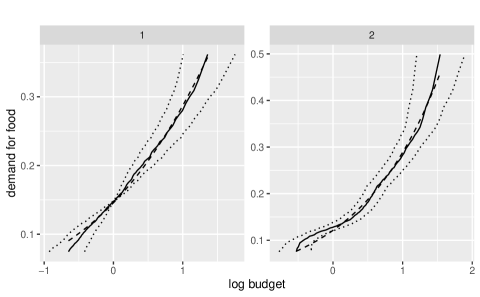
Figure 8.1: Estimated demand functions. Solid line is the nonparametric estimate, evaluated at the mean value of the demographics. The dotted lines indicate the 95% confidence interval. The dashed line is the PIGL closest to the nonparametric estimate. Left panel is for period 1, right panel is for period 2.

Table 1 gives our summary statistics (items 1-4 above), with bootstrapped 95% confidence intervals, for our estimates with 8 Bernstein polynomials (see the Appendix for other lengths of the Bernstein sieve). In the lower panel, we provide estimated regression coefficients, also with bootstrapped 95% confidence intervals, where we regress estimated resource shares $\widehat{\eta}_{i}$ on log-budgets $\overline{X}_{i}$ and demographics $z_{i}$.

	Estimate	q(2.5)	q(97.5)
$n=871$
Variability of fixed effects $\alpha_{i}$
$\hat{std}\left(\alpha_{i}\right)$	0.2647	0.1518	0.3707
$\hat{std}\left(e_{i}\right)$	0.1637	0.1262	0.1931
$\hat{cov}\left(\alpha_{i},X_{i1}\right)$	-0.0901	-0.1292	-0.0429
$\hat{cov}\left(\alpha_{i},X_{i2}\right)$	-0.1034	-0.1418	-0.0561
$\hat{std}\left(\alpha_{i}+X_{i1}\right)$	0.3537	0.2720	0.4605
$\hat{std}\left(\alpha_{i}+X_{i2}\right)$	0.3763	0.3010	0.4760
Regression estimates
$R^{2}$: $\overline{X}_{i},z_{i}$ on $\eta_{i}$	0.5205	0.3361	0.6508
$\overline{X}_{i}$	-0.0452	-0.0700	-0.0196
age–woman	-0.2513	-0.4437	-0.0545
age–man	0.2845	0.1389	0.4191
2 children	-0.0502	-0.1694	0.0413
3 or 4 children	-0.1248	-0.2407	0.0140
avg age of children	-0.0095	-0.1979	0.2151
fraction girl children	0.0136	-0.0881	0.1246
education–woman	-0.0325	-0.1519	0.1198
education–men	-0.1330	-0.2589	-0.0015

Table 1: Estimates.

Starting with the top panel of Table 1, the standard deviation of $\alpha_{i}$ is a measure of inter-household dispersion in women’s resource shares. If this dispersion is very small, then variation in resource shares does not induce much inequality, and we can reasonably use the household-level income distribution as a proxy for person-level inequality. However, if the dispersion is large, then household-level measures of inequality could be very misleading. Note here that we focus on inequality among women, not on gender inequality, precisely because the location of resource shares is not identified.

The estimated value is roughly $0.26$, with a 95% confidence interval covering roughly $0.15$ to $0.37$. To get a sense of the magnitude for the standard deviation of logged resource shares, suppose that women’s resource shares were lognormally distributed. Then our estimated standard deviation of 0.26 is consistent with 95% of the distribution of the resource shares lying in the range $[0.25,0.75]$, which represents quite a bit of heterogeneity across households.

The next row of Table 1 considers how much of the variation in $\alpha_{i}$ we can explain with observed covariates. The standard deviation of $e_{i}$ gives a measure of the unexplained variation, and gives us an idea of whether household-level unobserved heterogeneity is an important feature of the data. If the standard deviation of $e_{i}$ is very small, then fixed effects are not needed—conditioning on observed covariates would be sufficient. Our estimate of the standard deviation of the unexplained variation in $\alpha_{i}$ is about $0.16$. This is large relative to the overall estimated standard deviation of $0.26$, and suggests that accounting for household-level unobserved heterogeneity is quite important.

The next two rows give the covariance of $\alpha_{i}$ and $X_{it}$. Here, we see that log resource shares $\alpha_{i}$ strongly and statistically significantly negatively covary with observed household budgets (the implied correlation coefficients are close to $-0.8$). This means that women in poor households are somewhat less poor than they appear (on the basis of their household budget), and women in richer households are somewhat more poor than they appear. This is consistent with households that are closer to subsistence having a more equal distribution of resources.

The next two rows give the estimated standard deviation of women’s log shadow budgets. This is a scale-free parameter: it does not depend on the location normalization of $\alpha_{i}$ (which corresponds to a scale normalization of shadow budgets). The estimated standard deviations are $0.35$ and $0.38$ in the two periods, respectively. We can compare these with the standard deviation of log-budgets, reported in Table 1, of $0.49$ and $0.53$. The point estimates suggest that there is less inequality in women’s shadow budgets than in household budgets. Although the confidence intervals are large, the test of the hypothesis that the standard deviation of log-budgets equals the standard deviation of log-shadow budgets rejects in both years.

Thus, if we take these results at face value, there is less consumption inequality among women than household-level analysis would suggest. However, another implication of this is that there is more gender inequality than household level data would suggest. The reason is that household-level analysis of gender inequality pins gender inequality on over-representation of one gender in poorer households. In our data, all households have 1 man and 1 woman, so household-level analysis of gender inequality would show zero gender inequality. But, because women in richer households have smaller resource shares, this induces gender inequality even in these data.

Finding correlation between $\alpha_{i}$ and household budgets is not sufficient to invalidate previous identification strategies for cross-sectional settings that rely on independence between resource shares and household budgets. The reason is that the independence required is conditional on other observed covariates. To get a handle on this, the bottom panel of Table 1 presents estimates of coefficients in a linear regression of normalized (to average $0.33$) estimated resource shares $\widehat{\eta}_{i}$ on log-budgets $\overline{X}_{i}$ and other covariates $z_{i}$.

The figure below shows the scatterplot of predicted resource shares versus the log household budget. Here, we see a lot of variation in resource shares, and it is clearly correlated with household budgets. The overall variation here provides an estimate of the explained sum of squares in an infeasible regression of true resource shares $\eta_{i}$ on $\overline{X}_{i}$ and $z_{i}$. We may construct an estimate of the total sum of squares of resource shares from our estimate of the standard deviation of $\alpha_{i}$. This yields an estimate of $R^{2}$ in the infeasible regression, which we interpret as the fraction of variation in resource shares explained by observables.

Figure 8.2: Scatterplot of predicted resource shares and log budget.

In the first row of the bottom panel, we see that observed variables explain roughly half the variation in resource shares (the estimate of $R^{2}$ is $0.52$). This magnitude of explained variation is very close to that reported in Dunbar et al., 2019b in their cross-sectional estimate based on Malawian data. However, whereas the estimate in Dunbar et al., 2019b is conditional on the assumption that unobserved heterogeneity in resources shares is independent of the household budget, our estimate allows for correlation of resource shares with the household budget. This large magnitude of unexplained variation (roughly half) suggests that accounting for unobserved heterogeneity in resource shares is quite important.

Consider first the coefficient on $\overline{X}_{i}$. The estimated coefficient is $-0.045$ and is statistically significantly different from $0$. This means that, even after conditioning on other covariates (many of which are highly correlated with the budget), we still see a significant relationship between resource shares and household budgets.

However, the magnitude of this effect is small. Conditional on $z_{i}$, the standard deviation of $X_{it}$ is $0.43$ in year 1 and $0.47$ in year 2. Thus, comparing two households with identical $z$ but which are one standard deviation apart in terms the household budget, we would expect the woman in the poorer household to have a resource share $2$ percentage points higher than the woman in the richer household. Thus, the bulk of the variation that makes the standard deviation of women’s shadow budgets smaller than that of household budgets is not running through the dependence of resource shares on household budgets, but rather through the dependence of resource shares on other covariates that are correlated with household budgets.

We get a very precise estimate of the conditional dependence of resource shares on household budgets. Overall, then, we see that women’s resource shares are statistically significantly correlated with household budgets, even conditional on other observed characteristics. But, the estimated difference in resource shares at different household budgets is quite small. So, we take this as evidence that the identifying restrictions used by Dunbar et al., (2013) (and Dunbar et al., 2019b ) may be false, though perhaps not very false. It does suggest that alternative identifying restrictions—such as those developed here with a panel model—may be useful.

The rows of Table 1 give several other coefficients that are comparable to other estimates in the literature. Calvi, (2019) finds that women’s resource shares in India decline with the age of the woman. In these Bangladeshi data, we find evidence that women’s resource shares are strongly negatively correlated with the age of women and positively correlated with the age of men.

Dunbar et al., (2013) find that women’s resource shares in Malawi decline with the number of children. Here, we also see that pattern: households with 2 children have women’s resource shares $5$ percentage points less than households with 1 child; households with 3 or 4 children have resource shares $12$ percentage points less. Dunbar et al., (2013) also find that Malawian women’s resource shares are higher in households with girls than households with boys. We do not see evidence of this in rural Bangladesh: the estimated coefficient on the fraction of children that are girls statistically insignificantly different from $0$.

In the Appendix, we also provide estimates analogous to Table 1 using a different assignable good: clothing. Under the model, using different assignable goods should yield the same estimates of resource shares. This is roughly what we find in our estimates using women’s clothing.

Our estimates use 8th order Bernstein polynomials to approximate the inverse demand functionsD. In Appendix B, we present estimates using Bernstein polynomials of order $K=1,4,8,10$ and show that our finite-dimensional parameter estimates have roughly the same value for $K\geq 8$.

In summary, in these rural Bangladeshi households, we find evidence that women’s resource shares have substantial dependence on household-level unobserved heterogeneity and are slightly negatively correlated with household budgets. The former suggests that random-effects type approaches to the estimation of resource shares may be inadequate. The latter suggests that consumption inequality faced by women is actually smaller than household-level consumption inequality. It also suggests that cross-sectional identification strategies invoking independence of resource shares from household budgets, such as Dunbar et al., (2013), could be complemented by panel-based identification strategies such as ours.

ONLINE APPENDICES

Appendix A Proofs

A.1 Proof of Lemma (1)

Proof.

Define $\overline{D}=1\left\{D_{1}\left(y_{1}\right)+D_{2}\left(y_{2}\right)=1\right\}$. The proof consists in showing the following:

$$\text{med}\left(D_{2}\left(y_{2}\right)-D_{1}\left(y_{1}\right)|X,\overline{\,D}=1\right)$$ (A.1)

$$= \text{sgn}\left(P\left(D\left(y_{1},y_{2}\right)=\left(0,1\right)|X,\overline{\,D}=1\right)-P\left(D\left(y_{1},y_{2}\right)=\left(1,0\right)|X,\overline{\,D}=1\right)\right)$$ (A.2)

$$= \text{sgn }\left(\frac{P\left(D\left(y_{1},y_{2}\right)=\left(0,1\right),\overline{\,D}=1|X\right)}{P(\overline{D}=1|X)}-\frac{P\left(D\left(y_{1},y_{2}\right)=\left(1,0\right),\,\overline{D}=1|X\right)}{P(\overline{D}=1|X)}\right)$$ (A.3)

$$= \text{sgn }\left(P\left(D\left(y_{1},y_{2}\right)=\left(0,1\right),\overline{\,D}=1|X\right)-P\left(D\left(y_{1},y_{2}\right)=\left(1,0\right),\overline{\,D}=1|X\right)\right)$$ (A.4)

$$= \text{sgn}\left(P\left(D\left(y_{1},y_{2}\right)=\left(0,1\right)|X\right)-P\left(D\left(y_{1},y_{2}\right)=\left(1,0\right)|X\right)\right)$$ (A.5)

$$= \text{sgn}\left(P\left(D_{2}\left(y_{2}\right)=1|X\right)-P\left(D_{1}\left(y_{1}\right)=1|X\right)\right)$$ (A.6)

$$= \text{sgn}\left(\Delta X\beta-\gamma\left(y_{1},y_{2}\right)\right)$$ (A.7)

where $\left(\ref{eq:M2}\right)$ follows since the random variable $D_{2}\left(y_{2}\right)-D_{1}\left(y_{1}\right)\in\left\{-1,1\right\}$, which implies that

$$\text{med}\left(D_{2}\left(y_{2}\right)-D_{1}\left(y_{1}\right)|X,\overline{\,D}=1\right)$$

$$= \left\{\begin{array}[]{c}1\text{ if }P\left(D\left(y_{1},y_{2}\right)=\left(0,1\right)|X,\,\overline{D}=1\right)>P\left(D\left(y_{1},y_{2}\right)=\left(1,0\right)|X,\,\overline{D}=1\right)\\ -1\text{ if }P\left(D\left(y_{1},y_{2}\right)=\left(0,1\right)|X,\,\overline{D}=1\right)<P\left(D\left(y_{1},y_{2}\right)=\left(1,0\right)|X,\,\overline{D}=1\right)\end{array},\right.$$

$\left(\ref{eq:inbetween23}\right)$ follows from the definition of conditional probability, $\left(\ref{eq:alsoinbetween23}\right)$ follows since the sign function is not affected by scaling both quantities by the same positive factor (the denominator), $\left(\ref{eq:M3}\right)$ follows by the definition of $\overline{\,D}$, and $\left(\ref{eq:M4}\right)$ follows since:

$$P\left(D_{2}\left(y_{2}\right)=1|X\right) = P\left(D\left(y_{1},y_{2}\right)=\left(0,1\right)|X\right)+P\left(D\left(y_{1},y_{2}\right)=\left(1,1\right)|X\right)$$

$$P\left(D_{1}\left(y_{1}\right)=1|X\right) = P\left(D\left(y_{1},y_{2}\right)=\left(1,0\right)|X\right)+P\left(D\left(y_{1},y_{2}\right)=\left(1,1\right)|X\right)$$

Finally, $\left(\ref{eq:M5}\right)$ follows from Assumption 2(ii), which implies that, e.g.,

$$P\left(D_{2}\left(y_{2}\right)=1|\alpha,X\right) >P\left(D_{1}\left(y_{1}\right)=1|\alpha,X\right)\Leftrightarrow\alpha+X_{2}\beta-h_{2}^{-}\left(y_{2}\right)>\alpha+X_{1}\beta-h_{1}^{-}\left(y_{1}\right).$$

Integrating both sides over the conditional distribution of $\alpha$ given $X$ obtains:

$$P\left(D_{2}\left(y_{2}\right)=1|X\right)>P\left(D_{1}\left(y_{1}\right)=1|X\right) \Leftrightarrow X_{2}\beta-h_{2}^{-}\left(y_{2}\right)>X_{1}\beta-h_{1}^{-}\left(y_{1}\right)$$

$$\Leftrightarrow \Delta X\beta-\gamma\left(y_{1},y_{2}\right)>0.$$

Result $\left(\ref{eq:med_sgn}\right)$ now follows. ∎

A.2 Proof of Theorem 1

Proof.

Following Manski, (1985), it suffices to show that for an arbitrary $\theta\in\Theta$, $\theta\neq\theta_{0}\equiv\theta_{0}\left(y_{1},y_{2}\right)$,

$$P\left(W\theta<0\leq W\theta_{0}\right)+P\left(W\theta_{0}<0\leq W\theta\right)>0.$$ (A.9)

Our proof follows very closely that in Manski, (1985), with $W\theta$ taking the role of $xb$ and $W\theta_{0}$ taking the role of $x\beta$. However, our scale normalization is different.

Without loss of generality, let $X_{K}$ be the continuous regressor in Assumption 3(i). Separate $\Delta X=\left(\Delta X_{-K},\Delta X_{K}\right)$ where the first component $\Delta X_{-K}$ represents all covariates except the $K$-th one. Similarly, for any $\theta=\left(\beta,\gamma\right)\in\Theta$, separate $\beta=\left(\beta_{-K},\beta_{K}\right)$. Furthermore denote $W_{-K}=\left(\Delta X_{-K},-1\right)$ and $\theta_{-K}=\left(\beta_{-K},\gamma\right)$.

Assume that the associated regression coefficient $\beta_{0,K}>0$. The case $\beta_{0,K}<0$ follows similarly. Let $\theta=\left(\beta,\gamma\right)\in\Theta$, $\theta\neq\theta_{0}$. As in Manski (1985, p. 318), consider three cases: (i) $\beta_{K}<0$; (ii) $\beta_{K}=0$; (iii) $\beta_{K}>0$.

Cases (i) and (ii). $\beta_{K}\leq 0$. The proof is identical to that in Manski (1985), with $X\beta$ replaced by $W\theta$. The fact that we use a different scale normalization does not come into play.

Case (iii). $\beta_{K}>0$. note that

$$P\left(W\theta<0\leq W\theta_{0}\right) =P\left(-\frac{W_{-K}\theta_{0,-K}}{\beta_{0,K}}<\Delta X_{K}<-\frac{W_{-K}\theta_{-K}}{\beta_{K}}\right).$$

$$P\left(W\theta_{0}<0\leq W\theta\right) =P\left(-\frac{W_{-K}\theta_{-K}}{\beta_{K}}<\Delta X_{K}<-\frac{W_{-K}\theta_{0,-K}}{\beta_{0,K}}\right).$$

By assumption 4, $\frac{\beta_{-K}}{\beta_{K}}\neq\frac{\beta_{0,-K}}{\beta_{0,K}}$, which shows that the first $K$ components of the vector $\theta$ are not a scalar multiple of the first $K$ components of the vector $\theta_{0}.$ Therefore, $\theta$ is not a scalar multiple of $\theta_{0}$. In particular, $\frac{\theta_{0,-K}}{\beta_{0,K}}\neq\frac{\theta_{-K}}{\beta_{K}}$. Additionally, assumption 3(ii) implies that $P\left(\frac{W_{-K}\theta_{0,-K}}{\beta_{0,K}}\neq\frac{W_{-K}\theta_{-K}}{\beta_{K}}\right)>0$. Hence at least one of the two probabilities above is positive so that (A.9) holds. ∎

A.3 Proof of Theorem 2

Proof.

Under Assumption 5, $h_{1}^{-}(y_{0})=0$. Using the pair $(y_{0},y_{2})$ for binarization thus obtains identification of

$$\gamma\left(y_{0},y_{2}\right) =h_{2}^{-}(y_{2})-h_{1}^{-}(y_{0})$$

$$=h_{2}^{-}(y_{2}).$$

By varying $y_{2}\in\mathcal{\underline{Y}}$, we identify the function $h_{2}^{-}$ from the binary choice models associated with $\left\{D\left(y_{0},y_{2}\right)=\left(D_{1}\left(y_{0}\right),D_{2}\left(y_{2}\right)\right),y_{2}\in\underline{\mathcal{Y}}\right\}$.

The pairs $(y_{0},y_{2})$ and $(y_{1},y_{2})$ identify the difference

$$\gamma\left(y_{0},y_{2}\right)-\gamma\left(y_{1},y_{2}\right) =(h_{2}^{-}(y_{2})-h_{1}^{-}(y_{0}))-(h_{2}^{-}(y_{2})-h_{1}^{-}(y_{1}))$$

$$=h_{1}^{-}(y_{1}).$$

By varying $y_{1}\in\mathcal{\underline{Y}}$ we therefore identify $h_{1}^{-}$.

Thus, the functions $h_{1}^{-}$ and $h_{2}^{-}$ are identified. Because of monotonicity of $h_{t}$ (Assumption 1), and because $\mathcal{Y}$ is known, $h_{t}^{-}$ contains all the information about the pre-image of $h_{t}$. Knowledge of the pre-image of a function is equivalent to knowledge of the function itself. Therefore, $h_{t}$ can be identified from $h_{t}^{-}$. ∎

A.4 Proof of Theorem (3)

Proof.

For the panel data binary choice model with logit errors, we obtain

$$P(D_{2}\left(y_{2}\right)=1|\overline{D}\left(y_{1},y_{2}\right)=1,X,\alpha)$$ (A.10)

$$=\frac{P(D_{2}\left(y_{2}\right)=1,\overline{D}\left(y_{1},y_{2}\right)=1|X,\alpha)}{P\left(\overline{D}\left(y_{1},y_{2}\right)=1|X,\alpha\right)}$$ (A.11)

$$=\frac{P(D_{1}\left(y_{1}\right)=0,D_{2}\left(y_{2}\right)=1|X,\alpha)}{P\left(\overline{D}\left(y_{1},y_{2}\right)=1|X,\alpha\right)}$$ (A.12)

$$=\frac{P(D_{1}\left(y_{1}\right)=0,D_{2}\left(y_{2}\right)=1|X,\alpha)}{P(D_{1}\left(y_{1}\right)=0,D_{2}\left(y_{2}\right)=1|X,\alpha)+P(D_{1}\left(y_{1}\right)=1,D_{2}\left(y_{2}\right)=0|X,\alpha)}$$ (A.13)

$$=\frac{1}{1+\frac{P(D_{1}\left(y_{1}\right)=1,D_{2}\left(y_{2}\right)=0|X,\alpha)}{P(D_{1}\left(y_{1}\right)=0,D_{2}\left(y_{2}\right)=1|X,\alpha)}}$$ (A.14)

$$=\Lambda(\Delta X\beta-\gamma(y_{1},y_{2}))$$ (A.15)

where A.11 follows from the definition of a conditional probability; A.12 follows because $D_{2}=1$ and $\bar{D}=1$ are equivalent to $D_{1}=0$ and $D_{2}=1;$ A.13 follows because $D_{1}+D_{2}=1$ happens precisely when either $\left(D_{1},D_{2}\right)=\left(1,0\right)$ or $\left(D_{1},D_{2}\right)=\left(0,1\right)$; A.14 follows by dividing by the numerator; and the final expression follows by the argument below.

Note that $\frac{P(D_{1}\left(y_{1}\right)=1,D_{2}\left(y_{2}\right)=0|X,\alpha)}{P(D_{1}\left(y_{1}\right)=0,D_{2}\left(y_{2}\right)=1|X,\alpha)}$ equals

$$\frac{P(D_{1}\left(y_{1}\right)=1|X,\alpha)P(D_{2}\left(y_{2}\right)=0|X,\alpha)}{P(D_{1}\left(y_{1}\right)=0|X,\alpha)P(D_{2}\left(y_{2}\right)=1|X,\alpha)}$$ (A.16)

$$=\frac{\Lambda\left(\alpha+X_{1}\beta-h_{1}^{-}(y_{1})\right)\left[1-\Lambda\left(\alpha+X_{2}\beta-h_{2}^{-}(y_{2})\right)\right]}{\left[1-\Lambda\left(\alpha+X_{1}\beta-h_{1}^{-}(y_{1})\right)\right]\Lambda\left(\alpha+X_{2}\beta-h_{2}^{-}(y_{2})\right)}$$ (A.17)

$$=\frac{\exp\left(\alpha+X_{1}\beta-h_{1}^{-}(y_{1})\right)}{\exp\left(\alpha+X_{2}\beta-h_{2}^{-}(y_{2})\right)}$$ (A.18)

$$=\exp\left(\left(X_{1}-X_{2}\right)\beta-\left(h_{1}^{-}(y_{1})-h_{2}^{-}(y_{2})\right)\right),$$ (A.19)

where A.16 follows from serial independence of $\left(U_{1},U_{2}\right)$ conditional on $\left(X,\alpha\right)$; A.17 from the logit model specification; and A.18 follows from

$$\Lambda\left(u\right)/\left(1-\Lambda\left(u\right)\right)=\exp\left(u\right).$$

The discussion above implies that A.10 does not depend on $\alpha$. Hence,

$$p\left(X,y_{1},y_{2}\right) \equiv P(D_{2}\left(y_{2}\right)=1|\overline{D}\left(y_{1},y_{2}\right)=1,X)$$

$$=\Lambda(\Delta X\beta-\gamma(y_{1},y_{2}))$$

$$=\Lambda\left(W\theta\left(y_{1},y_{2}\right)\right).$$

and note that $p\left(X,y_{1},y_{2}\right)$ is identified from the distribution of $\left(Y,X\right)$, which is assumed to be observed. Then

$$\theta(y_{1},y_{2})=[E(W^{\prime}W)]^{-1}E(W^{\prime}\Lambda^{-1}(p(X,y_{1},y_{2})))$$

by invertibility of $\Lambda$ and the full rank assumption on $E\left[W^{\prime}W\right]$. This establishes identification of $\beta$ and $\gamma\left(y_{1},y_{2}\right)$. The proof in Section A.3 applies, which shows the identification of $h_{1}$ and $h_{2}$. ∎

A.5 Proof of Theorems 4 and 5

Proof.

(a) Note that, without Assumption 5, it follows immediately from the proof of Theorem 2 that we can only identify $\left\{h_{t}^{-1}\left(y\right)-c_{1},y\in\mathcal{Y},t=1,2\right\}$, i.e. we identify the functions $g_{t}\left(y\right)$, $t=1,2.$

Because the functions $g_{1},g_{2}$ are identified, and because the distribution of $\left(Y,X\right)$ is observable, we can identify the distribution of the left hand side of the relation below:

$$g_{t}\left(Y_{t}\right)-X_{t}\beta =h_{t}^{-1}\left(Y_{t}\right)-X_{t}\beta-c_{1}$$

$$=\alpha-U_{t}-c_{1},$$

for $t=1,2$.

It follows that for all $x\in\mathcal{X},$

$$\mu\left(x\right) =E\left[\left.\alpha\right|X=x\right]$$

$$=E\left[\left.\alpha-U_{t}\right|X=x\right]+E\left[\left.U_{t}\right|X=x\right]$$

$$=E\left[\left.h_{t}^{-1}\left(Y_{t}\right)-X_{t}\beta\right|X=x\right]+m$$

$$=E\left[\left.g_{t}\left(Y_{t}\right)-X_{t}\beta\right|X=x\right]+c_{1}+m.$$

is identified up to the constants $c_{1}$ and $m$.

The difference in conditional means at any two values $x,x^{\prime}\in\mathcal{X}$ is therefore identified and given by:

$$\mu\left(x\right)-\mu\left(x^{{}^{\prime}}\right)=$$

$$\left(E\left[\left.g_{t}\left(Y_{t}\right)-X_{t}\beta\right|X=x\right]+c_{1}+m\right)-\left(E\left[\left.g_{t}\left(Y_{t}\right)-X_{t}\beta\right|X=x^{{}^{\prime}}\right]+c_{1}+m\right)$$

$$=E\left[\left.g_{t}\left(Y_{t}\right)-X_{t}\beta\right|X=x\right]-E\left[\left.g_{t}\left(Y_{t}\right)-X_{t}\beta\right|X=x^{{}^{\prime}}\right].$$

(b) To see that the conditional variance is identified, note that for all $x\in\mathcal{X},$

$$Cov\left(\left.g_{2}\left(Y_{2}\right)-X_{2}\beta,g_{1}\left(Y_{1}\right)-X_{1}\beta\right|X=x\right)=$$

$$=Cov\left(\left.h_{2}^{-1}\left(Y_{2}\right)-X_{2}\beta-c_{1},h_{1}^{-1}\left(Y_{1}\right)-X_{1}\beta-c_{1}\right|X=x\right)$$

$$=Cov\left(\left.\alpha-U_{1}-c_{1},\alpha-U_{2}-c_{1}\right|X=x\right)$$

$$=Var\left(\left.\alpha\right|X=x\right)-Cov\left(\left.\alpha,U_{1}\right|X=x\right)-Cov\left(\left.\alpha,U_{2}\right|X=x\right)+Cov\left(\left.U_{1},U_{2}\right|X=x\right)$$

$$=Var\left(\left.\alpha\right|X=x\right)=\sigma_{\alpha}^{2}\left(x\right),$$

where the first equality follows from the definition of $g_{t}$; the second from the model; the third equality follows from the linearity of the covariance; and the fourth equality uses assumption (4c) and (4d). ∎

Appendix B GMM Estimator

Botosaru and Muris, (2017) develop $\sqrt{n}$-asymptotically normal estimator for $\beta$ and (invertible) $h_{t}$ for the FELT model. For the empirical application in this paper, it is desirable to condition on household characteristics $z$. This extension is not covered by Botosaru and Muris, (2017). We describe here a GMM estimator that covers this case.

The women’s food demand equation (5.8) is a FELT model, conditional on observed covariates $z$. Denote the inverse demand functions $g_{t}(Y_{it},z_{it})=h_{t}^{-1}(\cdot,z_{it})$. Given (5.8) and a two-period setting with $t=1,2$, and time-invariant demographics $z_{it}=z_{i}$, we have

$$\alpha_{i}+X_{it}-U_{it}=g_{t}(Y_{it},z_{i}),$$ (B.1)

implying the conditional moment condition

$$E\left[\left.g_{2}(Y_{i2},z_{i})-g_{1}(Y_{i1},z_{i})-\triangle X_{it}\right|X_{i1},X_{i2},z_{i}\right]=0.$$ (B.2)

Sieve estimators. We approximate the inverse demand functions, $g_{t}$, $t=1,2,\text{ }$ using Bernstein polynomials. This allows us to impose monotonicity in a straightforward way, see, e.g., Wang and Ghosh, (2012). Let $k=0,...,K$ index univariate Bernstein functions denoted as $\mathcal{B}_{k}\left(\cdot,K\right)$, where $K$ is the degree of the Bernstein polynomial and where the Bernstein functions are given by:

$$\mathcal{B}_{k}\left(u,K\right)=\binom{K}{k}u^{k}\left(1-u\right)^{K-k},\,u\in\left[0,1\right].$$

Let $l=0,...,L$ index the elements of $z_{i}$, and let the first (index $0$) element of $z_{i}$ be a constant equal to 1, that is $z_{i}=\left[1,z_{i1},\dots,z_{iL}\right]$.

Our approximation to $g_{t}\left(Y_{it},z_{i}\right)$ is given by:

$$g_{t}\left(Y_{it},z_{i}\right) \approx\sum_{k=0}^{K}\beta_{kt}\left(z_{i}\right)\mathcal{B}_{k}\left(Y_{it},K\right)\approx\sum_{l=0}^{L}\sum_{k=0}^{K}z_{i}^{\left(l\right)}\beta_{kt}^{\left(l\right)}\mathcal{B}_{k}\left(Y_{it},K\right).$$

For example, when there are no covariates $L=0$, the expression above reduces to the standard Bernstein polynomial approximation $g_{t}\left(Y_{it}\right)\approx\sum_{k=0}^{K}\beta_{kt}^{\left(0\right)}\mathcal{B}_{k}\left(Y_{it},K\right).$ The Bernstein coefficients are linear functions of the demographics, and the dependence of the Bernstein coefficients on the demographics is allowed to vary with time. In this way, the relationship between the (nonlinear) demand $Y_{it}$ and the latent budget $Y_{it}^{*}$ depends on demographic characteristics and on prices, through $t$. Since Bernstein polynomials are defined on the unit interval, we normalize $Y_{it}$ to be uniform on $\left[0,1\right]$ by applying its empirical distribution function.

Unconditional moments. To form GMM estimators, we construct the following unconditional moments:

$$E\left[\left(\sum_{l=0}^{L}\sum_{k=0}^{K}z_{i}^{\left(l\right)}\left(\beta_{k2}^{\left(l\right)}\mathcal{B}_{k}\left(Y_{i2},K\right)-\beta_{k1}^{\left(l\right)}\mathcal{B}_{k}\left(Y_{i1},K\right)\right)-\triangle X_{it}\right)\mathcal{B}_{k^{\prime}}(x_{it},K)z_{i}^{\left(l^{\prime}\right)}\right]=0$$

for $k^{\prime}=0,\dots,K$, $l^{\prime}=0,\dots,L$, and $t=1,2$, and

$$E\left[\left(\sum_{l=0}^{L}\sum_{k=0}^{K}z_{i}^{\left(l\right)}\left(\beta_{k2}^{\left(l\right)}\mathcal{B}_{k}\left(Y_{i2},K\right)-\beta_{k1}^{\left(l\right)}\mathcal{B}_{k}\left(Y_{i1},K\right)\right)-\triangle X_{it}\right)X_{it}z_{i}^{\left(l^{\prime}\right)}\right]=0,$$

for $l^{\prime}=0,\dots,L$ and $t=1,2.$ We include the second condition (where the logged household budget $X_{it}$ is exogenous) because we ultimately wish to consider the correlation of $\alpha_{i}$ and $X_{it}$. For a given order of the sieve approximation, $K$, the equations above amount to a parametric linear GMM problem.

We impose increasingness on the estimates of the functions $g_{1}$ and $g_{2}$ by imposing $\beta_{kt}\left(z_{i}\right)\geq\beta_{k-1,t}\left(z_{i}\right),$ for all $z_{i}$, for all $t$, and for $k\geq 2$. This results in a quadratic programming problem with linear inequality restrictions, which we implement in R using the quadprog package.

Degree of Bernstein polynomial. Implementing this method requires the selection of the degree of the Bernstein polynomial, $K$. While developing a formal selection rule for this parameter would be desirable, it is beyond the scope of the present paper. Nonetheless, we adopt an informal selection rule for the number of Bernstein basis functions – the smoothing parameter – based on the following observation. In our semiparametric setting, the estimators are known to have the same asymptotic distribution for a range of smoothing parameters (see, e.g., Chen, (2007)). When the number of Bernstein basis functions is small, the bias dominates and the estimates exhibit a decreasing bias as the number of terms increases. On the other hand, when the number of basis functions is large, the statistical noise dominates. We implement our estimation method over a range of smoothing parameter values, that is, $K\in\left\{1,2,\dots,12\right\}$, in search of a region where the estimates are not very sensitive to small variations in the smoothing parameter. We select the mid-point of that region, so our main results use $K=8$. We present results for $K\in\left\{1,4,8,10\right\}$ in the Appendix. In the Appendix table, “X” denotes a case where an estimated variance is negative.

Confidence bands. The confidence bands presented here are computed via the nonparametric bootstrap. We acknowledge that these may not be valid as the shape constraints may be binding, see for example Andrews, (1999, 2000). Furthermore, they would have to reflect the choice of the order of the Bernstein polynomial. The theory to construct valid uniform confidence bands for our estimator is not yet available. We leave this as a topic for future research. Two possible solutions are to not impose monotonicity on the estimator for $h_{t}$ or to use a subset of households with fixed$-$z and implement the estimator proposed by Botosaru and Muris, (2017). Both monotonicity and accounting for household characteristics are essential components of our empirical application, so we do not pursue these approaches.

We use 1,000 bootstrap replications for all our results. We report pointwise 95% confidence bands. All reported estimates in the main text are bias-corrected using the bootstrap.

Estimates and parameters of interest. We present estimates for the demand functions, $\widehat{h}_{t}(x,\overline{z})=\widehat{g}_{t}^{-1}(\cdot,\overline{z})$ for $t=1,2$, where $\bar{z}$ represents a household with 1 child and has other observed characteristics that are the average of those of 1-child households. The functions $h_{t}$ (demand functions) are not of direct interest, but identification of the $h_{t}$ supports identification of moments of the distribution of fixed effects $\alpha_{i}$. In our context, $\alpha_{i}$ equals the log of the resource share of the woman in household $i$.

We characterize the following interesting features of the distribution of resource shares. Recall from Theorems 4 and 5 that identification of features of this distribution does not impose a normalization on assignable good demand functions, and only identifies the distribution of logged resource shares (fixed effects) up to location. Consequently, we only identify features of the resource share distribution up to a scale normalization.

Let $\widehat{g}_{it}=\widehat{g}_{t}(Y_{it},z_{i})$ equal the predicted values of the inverse demand functions at the observed data. Recall that $g_{t}\left(Y_{it},z_{i}\right)=\alpha_{i}+X_{it}-U_{it},$ so we can think of $\widehat{g}_{it}-X_{it}$ as a prediction of $\alpha_{i}-U_{it}$. We then compute the following summary statistics of interest, leaving the dependence of $\hat{g}_{it},\,t=1,2,$ on $z_{i}$ implicit:

1. an estimate of the standard deviation of $\alpha_{i}$ given by

   $$\hat{std}\left(\alpha\right)=\sqrt{\hat{cov}\left(\left(\widehat{g}_{i2}-X_{i2}\right),\left(\widehat{g}_{i1}-X_{i1}\right)\right)},$$

   where $\hat{cov}$ denotes the sample covariance. The standard deviation of logs is a standard (scale-free) inequality measure. So this gives a direct measure of inter-household variation in women’s resource shares.

2. an estimate of the standard deviation of the projection error, $e_{i},$ of $\alpha_{i}$ on $\bar{X}_{i}=\frac{1}{2}\left(X_{i1}+X_{i2}\right)$ and $Z_{i}$. Consider the projection

   $$\alpha_{i}=\gamma_{1}\bar{X}_{i}+\gamma_{2}Z_{i}+e_{i},$$

   where $Z_{i}$ contains a constant. We are interested in the standard deviation of $e_{i}$. To obtain this parameter, we compute estimators for $\gamma_{1},\gamma_{2}$ from the pooled linear regression of $\hat{g}_{it}-X_{it}$ on $\bar{X}_{i}\text{ and }Z_{i}.$ Call these estimators $\hat{\gamma}_{1},\hat{\gamma}_{2}$. Then, as in $\hat{std}\left(\alpha\right)$ in (1), an estimate of the standard deviation of $e_{i}$ is given by:

   $$\hat{std}\left(e_{i}\right)=\sqrt{\hat{cov}\left(\left(\widehat{g}_{i2}-X_{i2}-\hat{\gamma}_{1}\bar{X}_{i}-\hat{\gamma}_{2}Z_{i}\right),\left(\widehat{g}_{i1}-X_{i1}-\hat{\gamma}_{1}\bar{X}_{i}-\hat{\gamma}_{2}Z_{i}\right)\right)}.$$

   This object measures the amount of variation in $\alpha_{i}$ that cannot be explained with observed regressors. If it is zero, then we don’t really need to account for household-level unobserved heterogeneity in resource shares. It is much larger than zero, then accounting for household-level unobserved heterogeneity is important.

3. an estimate of the standard deviation of $\alpha_{i}+X_{it}$ for $t=1,2$, computed as

   $$\hat{std}\left(\alpha_{i}+X_{it}\right) =\sqrt{\hat{var}\left(\alpha_{i}\right)+\hat{var}\left(X_{it}\right)+2\hat{cov}\left(\alpha_{i},X_{it}\right)},$$

   where

   $$\hat{cov}\left(\alpha_{i},X_{i1}\right) =cov\left(\hat{g}_{i1}-X_{i1},X_{i1}\right),$$

   $$\hat{cov}\left(\alpha_{i},X_{i2}\right) =cov\left(\hat{g}_{i2}-X_{i2},X_{i2}\right),$$

   and $\hat{var}\left(\alpha_{i}\right)=\left(\hat{std}\left(\alpha\right)\right)^{2}$ and $\hat{var}\left(X_{it}\right),\,t=1,2,$ is observed in the data. Since $\alpha_{i}+X_{it}$ is a measure of the woman’s shadow budget, $\hat{std}\left(\alpha_{i}+X_{it}\right)$ is a measure of inter-household inequality in women’s shadow budgets. This inequality measure is directly comparable to the standard deviation of $X_{i}$ (shown in Table 1), which measures inequality in household budgets.

4. an estimate of the covariance of $\alpha_{i},X_{it}$ for $t=1,2$, denoted $\hat{cov}\left(\alpha_{i},X_{it}\right)$. This object is of direct interest to applied researchers using cross-sectional data to identify resource shares. If this covariance is non-zero, then the independence of resource shares and household budgets is cast into doubt, and identification strategies based on this restriction are threatened.

Of these, the first 2 summary statistics are about the variance of fixed effects, and are computed using data from both years. Their validity requires serial independence of the measurement errors $U_{it}$. In contrast, the second 2 summary statistics are about the correlation of fixed effects with the household budget, and are computed at the year level. They are valid with stationary $U_{it}$, even in the presence of serial correlation.

We also consider the multivariate relationship between resource shares, household budgets and demographics. Recall that the fixed effect $\alpha_{i}$ subject to a location normalization; this means that resource shares are subject to a scale normalization. So, we construct an estimate of the woman’s resource share in each household as $\widehat{\eta}_{i}=\exp\left(\frac{1}{2}\left(\hat{g}_{i1}-X_{i1}\right)+\left(\hat{g}_{i2}-X_{i2}\right)\right)$, normalized to have an average value of $0.33$. Then, we regress estimated resource shares $\widehat{\eta}_{i}$ on $\bar{X}_{i}$ and $Z_{i}$, and present the estimated regression coefficients, which may be directly compared with similar estimates in the cross-sectional literature.

The estimated coefficient on $X_{i}$ gives the conditional dependence of resource shares on household budgets, and therefore speaks to the reasonableness of the restriction that resource shares are independent of those budgets (an identifying restriction used in the cross-sectional literature). Finally, using the estimate of the variance of fixed effects, we construct an estimate of $R^{2}$ in the regression of resource shares on observed covariates. This provides an estimate of how much unobserved heterogeneity matters in the overall variation of resource shares.

We also provide estimates that use women’s clothing as the assignable non-shareable good. Here, clothing expenditure is equal to four times the reported three-month recall expenditure on the following female-specific clothing items: Saree; Blouse/ petticoat; Salwar kameez; and Orna. We note that although clothing is a semi-durable good, there are 3 years between the waves of the panel. Consequently, we do not think that the demands across periods will be strongly correlated due to the durability of clothing purchased.

Appendix table “Additional Estimates” gives results for $K\in\left\{1,4,8,10\right\}$ for food (top panel) and clothing (bottom panel). In the table, “X” denotes a case where an estimated variance is negative.

Appendix C Descriptive Statistics

Table 2: Descriptive Statistics
	raw data				top- and bottom-coded
$n=871$					and normalized
Variable	Mean	Std Dev	Min	Max	Mean	Std Dev
$X_{i1}$	11.68	0.49	10.24	13.68
$X_{i2}$	12.02	0.53	10.70	14.08
$\triangle X_{i}$	0.34	0.43	-0.94	2.31
$Y_{i1}$	1561	1277	0	13500
$Y_{i2}$	1912	1727	0	15000
age of woman	32.76	7.64	19.00	90.00	0.35	0.25
age of man	39.77	10.76	15.00	105.00	0.37	0.25
$2$ children	0.47	0.50	0.00	1.00	0.47	0.50
$3$ or $4$ children	0.19	0.39	0.00	1.00	0.19	0.39
age of children	8.37	2.75	1.00	14.00	0.50	0.25
fraction girl children	0.46	0.39	0.00	1.00	0.46	0.39
education of woman	4.10	3.43	0.00	10.00	0.44	0.37
education of man	3.41	3.74	0.00	10.00	0.34	0.37

Table 2: Summary statistics.

Appendix D Additional estimates

[H] 1 4 8 10 Estimate q(2.5) q(97.5) Estimate q(2.5) q(97.5) Estimate q(2.5) q(97.5) Estimate q(2.5) q(97.5) Variability in unobservables: Food sd_a 0.3574 0.2258 0.5025 0.3197 0.2210 0.4376 0.2647 0.1518 0.3707 0.2286 0.0462 0.3592 sd_e 0.1947 0.1401 0.2377 0.1845 0.1413 0.2202 0.1637 0.1262 0.1931 0.1631 0.1308 0.1908 sd_ax1 -0.0506 -0.0934 -0.0085 -0.0805 -0.1300 -0.0246 -0.0901 -0.1292 -0.0429 -0.0781 -0.1166 -0.0339 sd_ax2 -0.0549 -0.0979 -0.0129 -0.0832 -0.1313 -0.0277 -0.1034 -0.1418 -0.0561 -0.0930 -0.1310 -0.0497 cov_ax1 0.5159 0.4067 0.6465 0.4272 0.3279 0.5763 0.3537 0.2720 0.4605 0.3635 0.2846 0.4583 cov_ax2 0.5444 0.4489 0.6637 0.4636 0.3757 0.6107 0.3763 0.3010 0.4760 0.3822 0.3104 0.4781 Regression coefficients: Food $R^{2}:\overline{X}_{i},z_{i}$ on $\eta_{i}$ 0.6749 0.5292 0.8088 0.6341 0.4179 0.8026 0.5205 0.3361 0.6508 0.5369 0.3797 0.6447 $\overline{X}_{i}$ -0.0353 -0.0643 -0.0083 -0.0237 -0.0534 0.0039 -0.0452 -0.0700 -0.0196 -0.0481 -0.0731 -0.0234 age_women -0.1095 -0.4028 0.2182 -0.2807 -0.5228 -0.0498 -0.2513 -0.4437 -0.0545 -0.3438 -0.5891 -0.1424 age_men -0.0284 -0.3205 0.2123 0.1146 -0.0846 0.2811 0.2845 0.1389 0.4191 0.2904 0.1306 0.4392 children2 -0.1948 -0.3296 -0.0860 -0.1955 -0.3180 -0.0884 -0.0502 -0.1694 0.0413 -0.0821 -0.2229 0.0167 children3p -0.2134 -0.3372 -0.1132 -0.2231 -0.3440 -0.0991 -0.1248 -0.2407 0.0140 -0.1159 -0.2466 0.0197 age_children -0.3004 -0.5448 -0.0620 -0.0819 -0.2875 0.1477 -0.0095 -0.1979 0.2151 0.0949 -0.0910 0.3209 frac_girl -0.0338 -0.1724 0.1209 0.0674 -0.0487 0.2049 0.0136 -0.0881 0.1246 -0.0322 -0.1466 0.0854 edu_women 0.0250 -0.1319 0.1803 0.0012 -0.1546 0.2036 -0.0325 -0.1519 0.1198 -0.1096 -0.2278 0.0132 edu_men 0.0079 -0.1213 0.1533 -0.1385 -0.2764 0.0091 -0.1330 -0.2589 -0.0015 -0.0202 -0.1501 0.1298 Variability in unobservables: Cloth sd_a 0.4729 X 0.7989 0.4224 0.2622 0.6944 0.2690 0.1472 0.4265 0.2443 0.1142 0.3749 sd_e 0.2350 X 0.3936 0.2131 0.1139 0.2875 X X 0.1210 X X X sd_ax1 -0.1254 -0.2157 -0.0341 -0.0503 -0.1049 0.0304 -0.1394 -0.1745 -0.0994 -0.1659 -0.1964 -0.1340 sd_ax2 -0.1185 -0.2186 -0.0207 -0.0903 -0.1583 -0.0043 -0.1832 -0.2211 -0.1406 -0.1903 -0.2234 -0.1537 cov_ax1 0.4633 X 0.7828 0.5667 0.4144 0.8386 0.1927 X 0.4568 X X 0.3213 cov_ax2 0.5203 X 0.8248 0.5319 0.3654 0.8218 X X 0.4190 X X 0.3217 Regression coefficients: Cloth $R^{2}:\overline{X}_{i},z_{i}$ on $\eta_{i}$ 11.2428 10.9458 14.5224 0.3753 -0.0344 1.0855 0.8791 0.6307 1.2056 1.1260 0.9142 1.3417 $\overline{X}_{i}$ 0.1716 0.0975 0.2610 0.0015 -0.0509 0.0574 -0.0925 -0.1245 -0.0591 -0.1488 -0.1738 -0.1200 age_women 0.2658 -0.4693 1.1146 -0.3608 -0.6580 -0.0759 -0.2666 -0.4136 -0.0894 -0.1123 -0.2224 0.0056 age_men 0.1706 -0.3577 0.8011 0.5223 0.3033 0.8700 0.2860 0.1753 0.4254 0.1840 0.0961 0.2934 children2 -0.5101 -0.8971 -0.1832 0.0950 -0.0863 0.3863 0.0495 -0.0380 0.1572 0.0623 0.0008 0.1369 children3p -0.3017 -0.7165 0.2456 -0.1110 -0.2746 0.1671 -0.0377 -0.1448 0.2903 -0.0549 -0.1511 0.2868 age_children -1.1070 -1.7016 -0.5342 -0.0087 -0.2421 0.2433 0.0449 -0.0820 0.1722 -0.0925 -0.2044 -0.0050 frac_girl -0.0222 -0.3256 0.3410 -0.3711 -0.5782 -0.2411 0.0926 0.0196 0.1633 0.0620 0.0028 0.1103 edu_women -0.0821 -0.5592 0.3867 -0.0727 -0.2605 0.1185 -0.2170 -0.3154 -0.1348 -0.1029 -0.1815 -0.0414 edu_men -0.5244 -0.9658 -0.1072 0.0746 -0.1260 0.4180 0.0420 -0.0497 0.1742 0.0167 -0.0537 0.1036

Summary statistics for log resource shares and their projection on demographics and budget.

References

- Abrevaya, (1999) Abrevaya, J. (1999). Leapfrog estimation of a fixed-effects model with unknown transformation of the dependent variable. Journal of Econometrics, 93(2):203–228.
- Abrevaya, (2000) Abrevaya, J. (2000). Rank estimation of a generalized fixed-effects regression model. Journal of Econometrics, 95(1):1–23.
- Abrevaya and Muris, (2020) Abrevaya, J. and Muris, C. (2020). Interval censored regression with fixed effects. Journal of Applied Econometrics, 35(2):198–216.
- Ai and Gan, (2010) Ai, C. and Gan, L. (2010). An alternative root-n consistent estimator for panel data binary choice models. Journal of Econometrics, 157(1):93–100.
- Altonji and Matzkin, (2005) Altonji, J. G. and Matzkin, R. L. (2005). Cross section and panel data estimators for nonseparable models with endogenous regressors. Econometrica, 73(4):1053–1102.
- Andrews, (1999) Andrews, D. W. (1999). Estimation when a parameter is on a boundary. Econometrica, 67:1341–1383.
- Andrews, (2000) Andrews, D. W. (2000). Inconsistency of the bootstrap when a parameter is on the boundary of the parameter space. Econometrica, 68:399–405.
- Arellano and Bonhomme, (2009) Arellano, M. and Bonhomme, S. (2009). Robust priors in nonlinear panel data models. Econometrica, 77(2):489–536.
- Arellano and Bonhomme, (2011) Arellano, M. and Bonhomme, S. (2011). Nonlinear panel data analysis. Annual Review of Economics, 3(1):395–424.
- Arellano and Bonhomme, (2012) Arellano, M. and Bonhomme, S. (2012). Identifying distributional characteristics in random coefficients panel data models. Review of Economic Studies, 79(3):987–1020.
- Arellano and Hahn, (2007) Arellano, M. and Hahn, J. (2007). Understanding bias in nonlinear panel models: Some recent developments. In Blundell, R., Newey, W., and Persson, T., editors, Advances in Economics and Econometrics, pages 381–409.
- (12) Aristodemou, E. (forthcoming). Semiparametric identification in panel data discrete response models. Journal of Econometrics.
- Baetschmann et al., (2015) Baetschmann, G., Staub, K. E., and Winkelmann, R. (2015). Consistent estimation of the fixed effects ordered logit model. Journal of the Royal Statistical Society A, 178(3):685–703.
- Banks et al., (1997) Banks, J., Blundell, R., and Lewbel, A. (1997). Quadratic engel curves and consumer demand. Review of Economics and statistics, 79(4):527–539.
- Bargain et al., (2014) Bargain, O., Donni, O., and Kwenda, P. (2014). Intrahousehold distribution and poverty: Evidence from cote d’ivoire. Journal of Development Economics, 107:262–276.
- Bargain et al., (2018) Bargain, O., Lacroix, G., and Tiberti, L. (2018). Validating the collective model of household consumption using direct evidence on sharing. Partnership for Economic Policy Working Paper 2018-06.
- Becker, (1962) Becker, G. S. (1962). Investment in human capital: A theoretical analysis. Journal of Political Economy, 70(5):9–49.
- Berkson, (1950) Berkson, J. (1950). Are there two regressions? Journal of the American Statistical Association, 45(250):164–180.
- Bester and Hansen, (2009) Bester, C. A. and Hansen, C. (2009). Identification of marginal effects in a nonparametric correlated random effects model. Journal of Business and Economic Statistics, 27(2):235–250.
- Bonhomme, (2012) Bonhomme, S. (2012). Functional differencing. Econometrica, 800(4):1337–1385.