ScoreDrivenModels.jl: a Julia Package for
Generalized Autoregressive Score Models

Guilherme Bodin, Raphael Saavedra, Cristiano Fernandes, Alexandre Street ScoreDrivenModels.jl: Generalized Autoregressive Score Models in Julia ScoreDrivenModels.jl: Generalized Autoregressive Score Models in Julia Score-driven models, also known as generalized autoregressive score (GAS) models, represent a class of observation-driven time series models. They possess powerful properties, such as the ability to model different conditional distributions and to consider time-varying parameters within a flexible framework. In this paper, we present ScoreDrivenModels.jl, an open-source Julia package for modeling, forecasting, and simulating time series using the framework of score-driven models. The package is flexible with respect to model definition, allowing the user to specify the lag structure and which parameters are time-varying or constant. It is also possible to consider several distributions, including Beta, Exponential, Gamma, Lognormal, Normal, Poisson, Student’s t, and Weibull. The provided interface is flexible, allowing interested users to implement any desired distribution and parametrization. score-driven models, generalized autoregressive score models, time series models, time-varying parameters, non-Gaussian models score-driven models, generalized autoregressive score models, time series models, time-varying parameters, non-Gaussian models Guilherme Bodin (corresponding author)
Department of Electrical Engineering
Pontifícia Universidade Católica do Rio de Janeiro
R. Marquês de São Vicente, 225
Gávea, Rio de Janeiro - RJ, Brazil
E-mail:

Raphael Saavedra
Invenia Labs
95 Regent St
Cambridge CB2 1AW, United Kingdom
E-mail:

Cristiano Fernandes
Department of Electrical Engineering
Pontifícia Universidade Católica do Rio de Janeiro
R. Marquês de São Vicente, 225
Gávea, Rio de Janeiro - RJ, Brazil
E-mail:

Alexandre Street
Department of Electrical Engineering
Pontifícia Universidade Católica do Rio de Janeiro
R. Marquês de São Vicente, 225
Gávea, Rio de Janeiro - RJ, Brazil
E-mail:

1 Introduction

Time series models with time-varying parameters have become increasingly popular over the years due to their advantages in capturing dynamics of series of interest. According to cox1981parameterdriven, the mechanism driving parameter dynamics in this general class of models can be of two types: parameter-driven, as in state space models (durbin2012time; koopman2000stamp; saavedra2019statespacemodels), or observation-driven. In this work, we will focus on a recently proposed class of observation-driven models wherein the score of the predictive density is used as the driver for parameter updating (creal2013generalized; harvey2013dynamic). These models have been referred to as generalized autoregressive score (GAS) models, dynamic conditional score models, or simply score-driven models. Additionally, it has been demonstrated that well-established observation driven models, such as the GARCH (bollerslev1986generalized) and conditional duration models (engle1998duration), are particular cases of the score-driven framework.

Two of the main advantages of the GAS framework are its ability to consider different non-Gaussian distributions and its flexibility with respect to the updating mechanism, which is determined by the chosen distribution determines the model updating mechanism. These properties have led GAS models to be applied in numerous fields, such as finance (harvey2016testing; ayala2018score), actuaries (Neves2017; demelo2018forecasting), risk analysis (patton2019dynamic; nani2019value), and renewable generation (saavedra2017study; Hoeltgebaum2018). We also refer the interested reader to a large online repository of works on GAS models at http://www.gasmodel.com. This wide range of applications has motivated the development of software packages for this class of models. For instance, there are open-source packages in Python (pyfluxTaylor), R (Ardia2019), and, recently, the data consultancy company Nlitn have made publicly available the Time Series Lab (https://timeserieslab.com), a free software developed by some of the authors of the theory developed in (creal2013generalized; harvey2013dynamic).

In this paper, we present a novel open-source GAS package fully implemented in Julia (bezanson2017julia) named ScoreDrivenModels.jl (bodin2020gas). One of Julia’s main advantages is to avoid the so-called two-language problem, i.e., the dependence on subroutines implemented in lower-level languages such as C/C++ or Fortran. Julia achieves this by providing a high-level programming syntax that allows for rapid prototyping and development without sacrificing computational performance. Thus, by providing an open-source package completely written in Julia, we facilitate development and contributions by users while also maintaining a high level of code transparency. The package allows users to specify a wide variety of GAS models by choosing the conditional distribution, the autoregressive structure, and which parameters are time-varying. Finally, initialization procedures are implemented to turn the estimation process more robust for the case of seasonal time series.

The remainder of this paper is organised as follows. Section 2 provides a brief overview of the GAS framework. In Section 3, the ScoreDrivenModels.jl package is presented, including the model specification, estimation, forecasting, and simulation. Section 4 presents examples of applications to illustrate the use of the package. Conclusions are drawn in Section LABEL:sec:conclusion. Finally, the Appendix provides the derivation of the score for each implemented distribution.

2 Score-Driven Models

2.1 The GAS Framework

Let $y_{t}\in\mathbb{Y}\subseteq\mathbb{R}$ denote the dependent variable of interest, $f_{t}\in\mathcal{P}\subset\mathbb{R}^{k}$ be a vector of time-varying parameters, and $Y^{t}=\{y_{1},\dots,y_{t}\}$ and $F^{t}=\{f_{0},f_{1},\dots,f_{t}\}$ denote the sets of available information until time $t$. We assume that $y_{t}$ is generated by the probability density function conditioned on the available information (past data and time-varying parameters) and on the hyperparameter vector $\theta$, which contains the constant parameters. It follows that the predictive distribution of $y_{t}$ has a closed form, represented as:

$$p(y_{t}|F^{t},Y^{t-1};\theta)$$ (1)

In score-driven models, the updating mechanism for the time-varying parameters $f_{t}$ is given by the following equation, referred to as a GAS($p$, $q$) mechanism:

$$f_{t+1}=\omega+\sum_{i=1}^{p}A_{i}s_{t-i+1}+\sum_{j=1}^{q}B_{j}f_{t-j+1},$$ (2)

where $\omega$ is a vector of constants, coefficient matrices $A_{i}$ and $B_{j}$ have appropriate dimensions for $i=1,\dots,p$ and $j=1,\dots,q$, and $s_{t}=s_{t}(y_{t},f_{t},F_{t-1},Y_{t-1};\theta)$ is an appropriate function of past data. The unknown coefficients in Eq. (2) are functions of the vector of hyperparameters $\theta$; that is, $\omega=\omega(\theta)$, $A_{i}=A_{i}(\theta)$, and $B_{j}=B_{j}(\theta)$. At instant $t$, the update of the time-varying $f_{t}$ for the next period $t+1$ is conducted through Eq. (2), with

$$s_{t}=\mathcal{I}_{t|t-1}^{-d}\cdot\nabla_{t},\quad\quad\nabla_{t}=\frac{\partial\ln p(y_{t}|f_{t},F_{t-1},Y_{t-1};\theta)}{\partial f_{t}},$$ (3)

where $\nabla_{t}$ is the called the score and $\mathcal{I}_{t|t-1}^{-d}$ is the scaled Fisher information of the probability density $p(y_{t}|f_{t},\mathcal{F}_{t-1};\theta)$. The scaling coefficient $d$ commonly takes values in $\{0,\frac{1}{2},1\}$. It is worth mentioning that in the case where $d=\frac{1}{2}$, it follows that $\mathcal{I}_{t|t-1}^{-\frac{1}{2}}$ results from the Cholesky decomposition of $\mathcal{I}_{t|t-1}^{-1}$.

As a consequence of the time-varying mechanism for the distribution parameters presented in Eq. (2), the conditional distribution of a GAS model is capable of continuously changing based on the considered data. For instance, if the time series contains occasional volatility spikes, the model can capture this behavior through the time-varying nature of the parameters. This property is illustrated in Fig. 1.

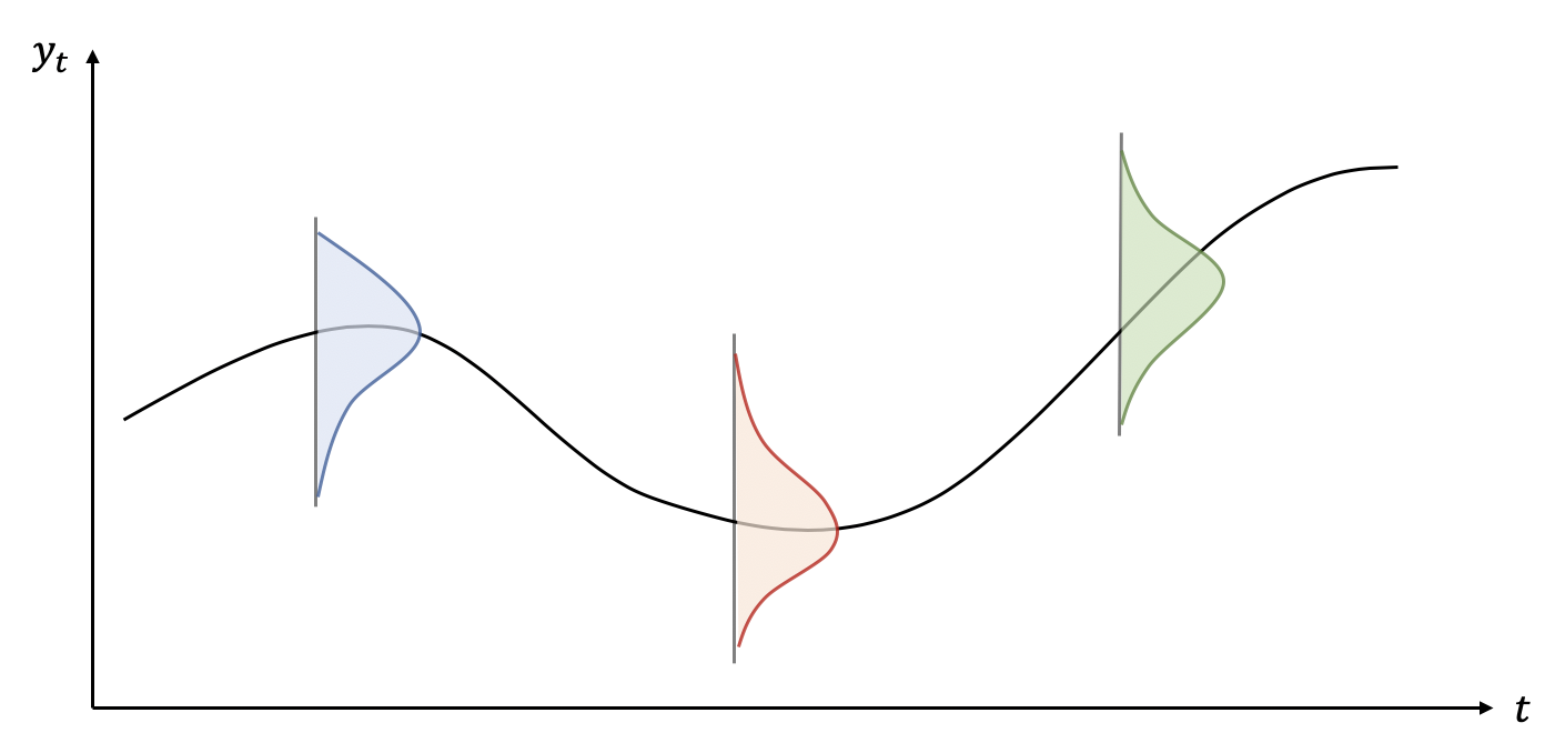
Figure 1: The GAS framework allows the conditional distribution to continuously change based on the data.

2.2 Parametrization

In the GAS updating mechanism (2), the parameter $f_{t}\in\mathcal{P}\subset\mathbb{R}^{k}$ is sometimes bounded – for example, in a Normal GAS model where the variance is time-varying, we would have $f_{t}=\sigma^{2}_{t}$ which can only assume positive values by definition. However, in some cases the recursion can lead to updates of $f_{t}\notin\mathcal{P}$. A solution is to reparametrize the equations in order to guarantee $f_{t}\in\mathcal{P}$ for every update. To that end, we follow the procedure described in creal2013generalized and present an example to illustrate it.

Let $f_{t}$ be the vector of time-varying parameters of a Normal distribution. From the properties of the distribution, it follows that $\mu_{t}\in\mathbb{R}$ and $\sigma^{2}_{t}\in\mathbb{R}^{+}$. Let us define a new time-varying parameter $\tilde{f}_{t}\in\mathbb{R}^{k}$ and a map $h:\mathcal{P}\to\mathbb{R}^{k}$, which we denote the link function in the package. In the case of the Normal distribution, a useful approach is to have an IdentityLink for $\mu_{t}$ and a LogLink for $\sigma^{2}_{t}$ as follows:

$$f_{t}=\begin{bmatrix}\mu_{t}\\ \sigma^{2}_{t}\end{bmatrix},\tilde{f}_{t}=\begin{bmatrix}\mu_{t}\\ \ln\sigma^{2}_{t}\end{bmatrix}$$ (4)

Note that the use of this parametrization will affect the recursion in Eq. (2) as well as the final expressions of $s_{t}$. Thus, let us derive the new recursion for the (2), but this time with the guarantee that every update of $f_{t}$ respects $f_{t}\in\mathcal{P}$. To that end, we also define the inverse map $h^{-1}(\cdot)$ denoted in the software as the unlink function: $f_{t}=h^{-1}(\tilde{f}_{t})$. Then, we can define the GAS updating recursion utilizing the parametrization:

$$\tilde{f}_{t+1}=\omega+\sum_{i=1}^{p}A_{i}\tilde{s}_{t-i+1}+\sum_{j=1}^{q}B_{j}\tilde{f}_{t-j+1}$$ (5)

The unknown coefficients in (5) remain as functions of $\theta$; that is, $\omega=\omega(\theta)$, $A_{i}=A_{i}(\theta)$, and $B_{j}=B_{j}(\theta)$. However, this time, we update the linked version of the time-varying parameters $\tilde{f}_{t}$ using (5). It is important to note that the expressions of $\tilde{s}_{t}$ are different for each scaling $d\in\{0,\frac{1}{2},1\}$. To compute these, we must use the derivative $\dot{h}$ of the map $h$, which is simply its Jacobian. In our example, $h$ is defined as

$$h\left(\begin{bmatrix}\mu_{t}\\ \sigma^{2}_{t}\end{bmatrix}\right)=\begin{bmatrix}h_{1}(\mu_{t})\\ h_{2}(\sigma^{2}_{t})\end{bmatrix}=\begin{bmatrix}\tilde{\mu}_{t}\\ \tilde{\sigma}^{2}_{t}\end{bmatrix}=\begin{bmatrix}\mu_{t}\\ \ln\sigma^{2}_{t}\end{bmatrix}$$ (6)

and its Jacobian is defined as

$$\dot{h}\left(\begin{bmatrix}\mu_{t}\\ \sigma^{2}_{t}\end{bmatrix}\right)=\begin{bmatrix}\frac{\partial h_{1}(\mu_{t})}{\partial\mu_{t}}&\frac{\partial h_{1}(\mu_{t})}{\partial\sigma^{2}_{t}}\\ \frac{\partial h_{2}(\sigma^{2}_{t})}{\partial\mu_{t}}&\frac{\partial h_{2}(\sigma^{2}_{t})}{\partial\sigma^{2}_{t}}\end{bmatrix}=\begin{bmatrix}1&0\\ 0&\frac{1}{\sigma^{2}_{t}}\end{bmatrix}$$ (7)

Note that $\dot{h}$ is always a diagonal matrix. The reparametrized score derivations for different scalings and different types of maps are presented in Appendix LABEL:appendix:parametrizations. Given the following definitions

$$\left.\dot{h}(f_{t})=\frac{\partial h(f_{t})}{\partial\tilde{f}_{t}}\right|_{f_{t}},\qquad\mathcal{J}_{t|t-1}\mathcal{J}_{t|t-1}^{\top}=\mathcal{I}_{t|t-1}^{-1},\qquad\tilde{\nabla}_{t}=\left(\dot{h}\right)^{-1}\nabla_{t},$$ (8)

then the linked scaled score $\tilde{s}_{t}$ can be computed as follows:

$$\tilde{s}_{t} =\left(\dot{h}\right)^{-1}\nabla_{t},\text{ for }d=0,$$ (9)

$$\tilde{s}_{t} =\mathcal{J}_{t|t-1}\nabla_{t},\text{ for }d=\frac{1}{2},$$ (10)

$$\tilde{s}_{t} =\dot{h}\mathcal{I}_{t|t-1}^{-1}\nabla_{t},\text{ for }d=1.$$ (11)

2.3 Maximum Likelihood Estimation

The vector of hyperparameters $\theta$ can be estimated via maximum likelihood:

$$\hat{\theta}={\arg\max}_{\theta}\sum_{t=1}^{N}\ln p(y_{t}|f_{t},\mathcal{F}_{t-1};\theta)$$ (12)

Evaluating the log-likelihood function of the GAS model is particularly simple. Given values for the constant parameters $\theta$, the GAS updating equation (2) outputs the conditional distribution at each time period, which generally has a closed form. Thus, it suffices to look at $\ln p(y_{t}|f_{t},\mathcal{F}_{t-1};\theta)$ for a particular value of $\theta$.

Evaluating the analytical derivatives needed to obtain the maximum likelihood is a demanding and sometimes impossible task. As a consequence, a common practice is to numerically evaluate derivatives using global optimization methods such as L-BFGS (liu1989limited) and Nelder-Mead (neldermead). Depending on the case, constrained optimization can also be applied, using, for instance, a Newton interior points method.

2.4 Forecasting

Forecasting and simulation of future scenarios are among the main goals in time series analysis. In Blasques2016, details of the procedure for out-of-sample confidence intervals for the time-varying parameters are discussed. The procedure discussed in Section 4.1 of Blasques2016 is currently implemented in ScoreDrivenModels.jl as follows:

1. Given $\hat{\theta}_{T}$ and the filtered state $\hat{f}_{T+1}$, draw $S$ values $y_{T+1}^{1},\dots,y_{T+1}^{S}$ from the estimated conditional density at $T+1$: $y_{T+1}\sim p(y_{T+1}|\hat{f}_{T+1},\hat{\theta}_{T})$ for $s=1,\dots,S$.

2. Use $y_{T+1}^{1},\dots,y_{T+1}^{S}$ and the recursion (2) to obtain the filtered values $\hat{f}_{T+2}^{1},\dots,\hat{f}_{T+2}^{S}$.

3. Repeat steps 1 and 2 $H$ times for $H$ steps ahead generating one new value of $y$ and $f$ per scenario $s$.

Once the procedure is over, $S$ scenarios for the observations within the entire horizon, $y_{T+k}^{s}$ for $k=1,\dots,H$ and $s=1,\dots,S$ have been simulated. Based on these set of scenario, one can calculate quantile forecasts, build empirical distributions, or use them to feed decision under uncertainty models, such as stochastic programming. Note that this method solely considers the uncertainty of innovations. The consideration of uncertainty on both innovations and parameters, as discussed in Blasques2016, is considered future work for the package.

3 The ScoreDrivenModels.jl Package

ScoreDrivenModels.jl enables users to create and estimate score-driven models and to perform forecasting and simulation while working purely in Julia. Its API allows users to choose between different distributions, scaling values, lag structures, and optimization methods. The basic code structure allows contributors to add new distributions and optimization methods; technical details about adding new features are available in the package documentation. Installation of the package is easily conducted using the Julia Package manager: pkg> add ScoreDrivenModels

3.1 Model Specification

To create a Model, the user must specify 1) the desired distribution, 2) the scaling, 3) the lag structure, and 4) which parameters should be considered time-varying.

1. The lag structure in a GAS($p,q$) model can be specified in two ways: either through integers p and q, which results in all lags from 1 to p and 1 to q being added, or through arrays of integers ps and qs containing only the desired lags.

2. To specify the distribution, the user needs to choose a distribution among the available ones that have an interface with Distributions.jl. The list of available distributions is displayed in Table 1. Furthermore, we refer the interested reader to Appendix LABEL:appendix:scores, where we provide details on the score calculations for each probability density made available in the package.

3. The scaling is specified by defining the value of $d$, which can be 0, 1, or $\frac{1}{2}$, respectively the identity scaling, inverse scaling, and inverse square-root scaling.

4. In order to define which distribution parameters should be time-varying, the keyword argument time_varying_params can be used. Note that the default behavior is to have all parameters as time-varying.

Distribution	Number of parameters	Identity scaling	Inverse scaling	Inverse square-root scaling
Beta	2	✓	✓	✓
BetaLocationScale	4	✓	–	–
Exponential	1	✓	✓	✓
Gamma	2	✓	✓	✓
LogitNormal	2	✓	✓	✓
LogNormal	2	✓	✓	✓
NegativeBinomial	2	✓	–	–
Normal	2	✓	✓	✓
Poisson	1	✓	✓	✓
TDist	1	✓	✓	✓
TDistLocationScale	3	✓	✓	✓
Weibull	2	✓	–	–

Table 1: List of currently implemented distributions and scalings. $\#$ represent the number of parameters of the distribution.

Once the model is specified, the unknown parameters that must be estimated are automatically represented as NaN within the Model structure. As an example, a GAS($1,2$) model with lognormal distribution and inverse square-root scaling can be created by writing the following line of code: julia> Model(1, 2, LogNormal, 0.5) ModelLogNormal,Float64([NaN, NaN], Dict(1=>[NaN 0.0; 0.0 NaN]), Dict(2=>[NaN 0.0; 0.0 NaN],1=>[NaN 0.0; 0.0 NaN]), 0.5)

Dict is the Julia data structure for dictionaries. Its use allows code flexibility enabling computational simplifications for complex lag structures. As displayed above, the unknown constant parameters to be estimated are set as NaN. In this case, the constant parameters considered in vector $\omega$ are $A_{1}$, $B_{1}$, and $B_{2}$.

In some applications, however, the user might define only one of the distribution parameters as time-varying. In the example below, the only time-varying parameter is $\mu_{t}$, so the keyword argument time_varying_params indicates a vector with only one element, [1], representing the first parameter of the lognormal distribution. A table that indicates the distribution parameters and their orders is available in the package documentation. The choice of the time-varying parameter can be expressed by the following code:

julia> Model(1, 2, LogNormal, 0.5; time_varying_params = [1]) ModelLogNormal,Float64([NaN, NaN], Dict(1=>[NaN 0.0; 0.0 0.0]), Dict(2=>[NaN 0.0; 0.0 0.0],1=>[NaN 0.0; 0.0 0.0]), 0.5) Users can also specify the lag structure by passing only the lags of interest. Note that this feature is equivalent to defining that matrices $A_{i}$ and $B_{j}$ are equal to zero for certain values $i$ and $j$. An example is a model that uses lags 1 and 12, which means that only the matrices $A_{1}$, $A_{12}$, $B_{1}$, and $B_{12}$ have nonzero entries:

julia> Model([1, 12], [1, 12], LogNormal, 0.5) ModelNormal,Float64([NaN, NaN], Dict(12=>[NaN 0.0; 0.0 NaN],1=>[NaN 0.0; 0.0 NaN]), Dict(12=>[NaN 0.0; 0.0 NaN],1=>[NaN 0.0; 0.0 NaN]), 0.5)

3.2 Estimation

Once the model is specified, the next step is estimation. Users can choose from different optimization methods provided by Optim.jl (mogensen2018optim). Since this optimization problem is non-convex, there is no guarantee that the optimal value found by the optimization method is the global optimum. To increase the chances of finding the global optimum, we run the optimization algorithm for different initial parameter values. The default method is Nelder-Mead with 3 random initial parameter values, but the optimization interface is highly flexible. Users can customize convergence tolerances, choose initial parameter values, and, depending on the optimization method, choose bounds for the parameters. By default, these initial values are the unconditional mean of $f_{t+1}$ which is given by

$$\E[f_{t+1}]=\omega\bigg{(}I-\sum_{j=1}^{q}B_{j}\bigg{)}^{-1}.$$ (13)

As an illustration, let us estimate a GAS model using the same data and specification used in the R package GAS (Ardia2019) paper with the function fit!, the data is also available in package repository (bodin2020gas). The data represents the monthly US inflation measured as the logarithmic change of the consumer price index. The model can be estimated as follows:

julia> Random.seed!(123) julia> y = vec(readdlm("../test/data/cpichg.csv")) julia> gas = Model(1, 1, TDistLocationScale, 0.0, time_varying_params=[1, 2]) julia> f = fit!(gas, y) Round 1 of 3 - Log-likelihood: -178.2064944794775 Round 2 of 3 - Log-likelihood: -178.20649327545632 Round 3 of 3 - Log-likelihood: -178.20649537930336

Users also have the option to check more detailed results of the optimization procedure by changing the keyword argument verbose. The default value of this argument is 1; to check the optimization summary, users should set the verbose level to 2, and to see the value of the objective function at each iteration of the optimization, it should be set to 3. To avoid the printing of outputs, users can set verbose = 0. To illustrate, results with level 2 is depicted below.

julia> gas = Model(1, 1, TDistLocationScale, 0.0, time_varying_params=[1, 2]) julia> f = fit!(gas, y; verbose=2) Round 1 of 3 - Log-likelihood: -178.20649402602353 Round 2 of 3 - Log-likelihood: -178.20649463073832 Round 3 of 3 - Log-likelihood: -178.2064932319776

Best initial_point optimization result: * Status: success

* Candidate solution Minimizer: [3.74e-02, -2.60e-01, 1.88e+00, …] Minimum: 1.782065e+02

* Found with Algorithm: Nelder-Mead Initial Point: [3.13e-02, 1.61e-01, 6.53e-02, …]

* Convergence measures standard-deviation <= 1.0e-06

* Work counters Seconds run: 0 (vs limit Inf) Iterations: 1345 f(x) calls: 2156

As mentioned before, while the maximization of the log-likelihood is done by default through the Nelder-Mead method with 3 random initial values, these features can be changed by the user. For example, to use the L-BFGS algorithm with 5 random initial values:

julia> gas = Model(1, 1, TDistLocationScale, 0.0, time_varying_params=[1, 2]) julia> f = fit!(gas, y; opt_method=LBFGS(gas, 5))

Once the estimation step is finished, the user can query the results by calling the function fit_stats:

julia> fit_stats(f) ——————————————————– Distribution: Distributions.LocationScaleFloat64, TDistFloat64 Number of observations: 276 Number of unknown parameters: 7 Log-likelihood: -178.2065 AIC: 370.4130 BIC: 395.7558 ——————————————————– Parameter Estimate Std.Error t stat p-value omega_1 0.0374 0.0311 1.2016 0.2686 omega_2 -0.2599 0.1409 -1.8454 0.1075 omega_3 1.8758 0.2914 6.4380 0.0004 A_1_11 0.0717 0.0184 3.8884 0.0060 A_1_22 0.4538 0.2139 2.1216 0.0715 B_1_11 0.9432 0.0272 34.6438 0.0000 B_1_22 0.8556 0.0743 11.5141 0.0000

This result matches the example discussed in Ardia2019 with the exception of omega_3, due to a difference in parametrization between the two packages. Once the parameter is recovered to its original parametrization, the result becomes the same.

3.3 Forecasting and Simulation

Forecasting in this framework is done by simulation as per Section 2.4. Function forecast runs the procedure proposed by Blasques2016 and returns a Forecast structure that has the expected value for time-varying parameters, observations, and the related scenarios used to find them. By default the structure also stores the 2.5%, 50% and 97.5% quantiles.

Next, we will present forecasting results using the previously estimated US inflation data. In the example below, the first column is the location parameter, the second column is the scale parameter, and the third column represents the degrees of freedom parameter.

julia> forec = forecast(y, gas, 12) julia> forec.parameter_forecast 12x3 ArrayFloat64,2: 0.101281 0.152362 6.52618 0.134314 0.159539 6.52618 0.165809 0.166048 6.52618 0.196427 0.171559 6.52618 0.219774 0.175267 6.52618 0.245018 0.17878 6.52618 0.267962 0.179805 6.52618 0.288717 0.182248 6.52618 0.308386 0.184336 6.52618 0.327622 0.185162 6.52618 0.348588 0.186111 6.52618 0.36383 0.186892 6.52618

We can also obtain the scenarios of observations, $y_{T+k}^{s}$ for $k=1,\dots,H$ and $s=1,\dots,S$, that generated the above forecasted values as follows:

julia> forec.observation_scenarios 12x10000 ArrayFloat64,2: 1.3839 -0.378146 … 0.561549 0.0415801 0.971144 0.116446 0.478346 0.290846 1.1637 0.439987 0.157433 -0.195271 0.50442 -0.0417178 0.204036 -0.549865 1.39936 0.149797 0.606875 -0.263888 1.04027 0.564609 … -0.234421 0.139999 0.609759 1.2166 0.236292 0.408869 0.693315 0.057054 0.802398 0.285412 0.908195 1.06543 1.22845 0.256618 1.89531 0.566139 0.808426 0.121839 1.7671 0.813116 … 0.639728 0.0408979 0.840164 0.72076 0.316973 0.300578

For the sake of clarity, the forecast $\hat{y}_{T+k}$ is the sample average of the scenarios of observations, i.e., $\hat{y}_{T+k}=S^{-1}\sum_{s=1}^{S}y_{T+k}^{s}$.

4 Applications

4.1 Hydropower Generation in Brazil

The Brazilian system operator regularly publishes an indicator of how much energy can be generated from water inflows among all hydropower plants in the country. This indicator is referred to as Affluent Natural Energy (ANE). Usually, ANE is computed in daily basis per region and then aggregated in a monthly basis as the average of each month.

Due to the high dependency of water resources, in Brazil, the monthly ANE is a key component of system operational and infrastructure planning studies. In most decision under uncertainty methodologies, it is essential to have simulated scenarios describing the empirical distribution rather than simple point forecasts.

In this section, we present an example that generates scenarios of the monthly aggregated ANE in the Northeastern region of Brazil illustrated in Fig. 2. This example employs a lognormal GAS model with tailored lag structure, identity scaling and time-varying parameter $\mu_{t}$. Finally, ANE scenarios are simulated based on the fitted hyperparameters.

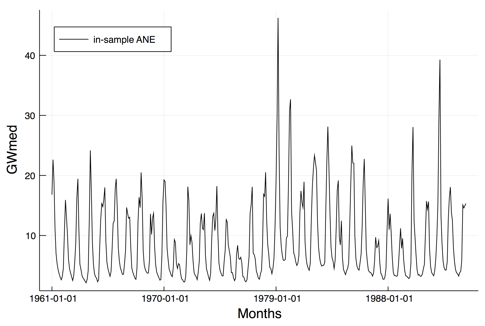
Figure 2: ANE in the Northeastern region of Brazil

In this model we utilize lags 1, 2, 11 and 12 for the score and autoregressive components; lags 1 and 2 capture the short-term trend of the series, while lags 11 and 12 capture the seasonal aspect of water inflow. The model can be written as follows:

$$\left\{\begin{array}[]{ccl}\mu_{t}&=&\omega_{1}+A_{1}s_{t-1}+A_{2}s_{t-2}+A_{11}s_{t-11}+A_{12}s_{t-12}\\ &&+B_{1}\mu_{t-1}+B_{2}\mu_{t-2}+B_{11}\mu_{t-11}+B_{12}\mu_{t-12}\\ \ln(\sigma^{2}_{t})&=&\omega_{2}\end{array}\right.$$ (14)

In this model we have also considered that the initial parameters $\mu_{1},\dots\mu_{12}$, $\sigma^{2}_{1},\dots,\sigma^{2}_{12}$, $s_{1},\dots s_{12}$ are calculated heuristically through maximum likelihood estimation in each seasonal component of the model. This way, the parameters $\mu_{1},\sigma_{1}$ are calculated by fitting a lognormal distribution in the observations $y_{1},y_{13},y_{25},\dots,y_{1+12n}$. This procedure was used in Hoeltgebaum2018. Note that this procedure, which is implemented by the function dynamic_initial_params in our package, is relevant for ensuring good estimation results when considering seasonal time series. The model is estimated as follows:

julia> Random.seed!(123) julia> y = vec(readdlm("../test/data/ane_northeastern.csv")) julia> y_train = y[1:400] julia> gas = Model([1, 2, 11, 12], [1, 2, 11, 12], LogNormal, 0.0; + time_varying_params=[1] julia> initial_params = dynamic_initial_params(y_train, gas) julia> f = ScoreDrivenModels.fit!(gas, y_train; initial_params=initial_params) julia> fit_stats(f) ——————————————————– Distribution: LogNormal Number of observations: 400 Number of unknown parameters: 10 Log-likelihood: -779.7883 AIC: 1579.5766 BIC: 1619.4912 ——————————————————– Parameter Estimate Std.Error t stat p-value omega_1 0.0135 0.0282 0.4807 0.6411 omega_2 -2.8408 0.0720 -39.4651 0.0000 A_1_11 -0.0378 0.0051 -7.4109 0.0000 A_2_11 0.0047 0.0034 1.4052 0.1903 A_11_11 -0.0178 0.0045 -3.9838 0.0026 A_12_11 0.0576 0.0052 11.0468 0.0000 B_1_11 -0.4784 0.0444 -10.7815 0.0000 B_2_11 0.4682 0.0449 10.4210 0.0000 B_11_11 -0.3055 0.0928 -3.2933 0.0081 B_12_11 1.3088 0.0962 13.6080 0.0000 Once the model is estimated we can generate 1000 ANE scenarios for the next 60 months following the methodology discussed in Section 2.4. We will utilize forecast in order to obtain the quantiles as well. The data set used to estimate the model used data from January 1961 until April 1994. To illustrate the adequacy of our model forecast, we present in Fig. 3 an out-of-sample study, where the simulated scenarios (gray lines), and related quantiles (red dotted lines) from May 1994 until April 1999 are contrasted to the actual observed values. julia> forec = forecast(y_train, gas, 60; S = 1_000, initial_params = initial_params)

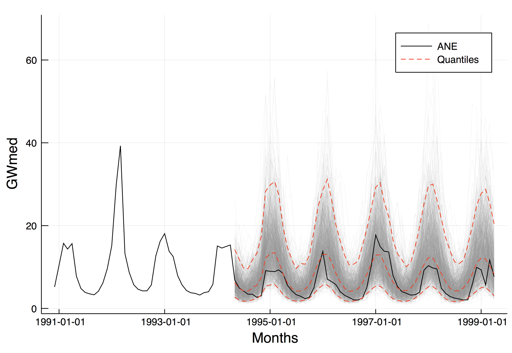
Figure 3: ANE scenarios in the Northeastern region of Brazil

4.2 GARCH Model

One of the advanced features of ScoreDrivenModels.jl is allowing users to change the default parametrization. An example of a different parametrization is the GARCH(1, 1) GAS model. It can be shown that a GAS(1, 1) is equivalent to a GARCH(1, 1) if the function $h$ is the identity (we refer the interested reader to Appendix LABEL:diffparam for further details). To ensure the equivalence, the user must define the identity link function for both time-varying parameters. To do this the user must overwrite three ScoreDrivenModel.jl methods as detailed in the following example: julia> function ScoreDrivenModels.link!(param_tilde::MatrixT, ::TypeNormal, param::MatrixT, t::Int) where T param_tilde[t, 1] = link(IdentityLink, param[t, 1]) param_tilde[t, 2] = link(IdentityLink, param[t, 2]) return end julia> function ScoreDrivenModels.unlink!(param::MatrixT, ::TypeNormal, param