Impurity induced scale-free localization

Abstract

This work develops a full framework for non-Hermitian impurity physics in a non-reciprocal lattice, with PBCs, OBCs and even their interpolations being special cases across a whole range of boundary impurity strengths. As the impurity strength is tuned, the localization of steady states can assume very rich behavior, including the expected non-Hermitian skin effect, Bloch-like states albeit broken translational invariance, and surprisingly, scale-free accumulation along or even against the direction of non-reciprocity. We further uncover the possibility of the co-existence of non-Hermitian skin effect and scale-free localization, where qualitative aspects of the system’s spectrum can be extremely sensitive to impurity strength. We have also proposed specific circuit setups for experimental detection of the scale-free accumulation, with simulation results confirming our main findings.

Spatial inhomogeneity in physical systems is the norm rather than the exception. It can trigger a wide variety of physical phenomena, such as the Anderson localization, topological edge states and topological defect states. In non-Hermitian systems, intriguing physics from spatial inhomogeneity encompasses not just the non-Hermitian skin effect (NHSE)Yao and Wang (2018); Yokomizo and Murakami (2019); Lee and Thomale (2019); Lee et al. (2018a); Kunst and Dwivedi (2019); Edvardsson et al. (2019); Yang et al. ; Zhang et al. (2019); Brandenbourger et al. (2019); Lee et al. (2019a); Mu et al. (2019); Li et al. (2019); Lee and Longhi (2020); Longhi (2020); Lee (2020); Cao et al. (2020); Xue et al. (2020); Liu et al. (2020); Rosa and Ruzzene (2020); Yoshida et al. (2020); Yi and Yang (2020); Xiao et al. (2020); Li et al. (2020); Schomerus (2020); Okuma et al. (2020); Koch and Budich (2020); Teo et al. (2020); Li et al. , but also impurity- or defect-induced topological bound states Bosch et al. (2019); Liu and Chen (2019); X. L. Zhao (2020); Liu and Chen , disorder-driven non-Hermitian topological phase transitions Luo and Zhang , as well as non-Hermitian quasi-crystals and mobility edges with an incommensurate modulation Longhi (2019); Jiang et al. (2019); Zeng et al. (2020); Claes and Hughes (2020).

Due to their emergent non-locality, non-reciprocal impurities in non-Hermitian systems generate dramatic spectral flows as their strengths are varied Xiong (2018); Lee and Thomale (2019). This has even been proposed for exponentially enhanced quantum sensing in an experimentally realistic setting Budich and Bergholtz ; McDonald and Clerk (2020). Yet, there does not exist a full framework for non-Hermitian impurity physics, with periodic and open boundary conditions (PBCs and OBCs) being special cases across a whole range of boundary impurity strengths. This work aims to fill in this important gap and reports unexpected findings of general theoretical and experimental interest.

Specifically, we discover that boundary impurities in non-reciprocal lattices can generate new types of steady-state localization behavior characterized by scale-free accumulation (SFA) of eigenstates, despite having non-power-law profile. In sharp contrast to the NHSE, the SFA direction can be counter-intuitive, opposite of the non-reciprocal directionality. With varying impurity strengths, the steady state makes transitions between the NHSE behavior, Bloch-like eigenstates with broken translational invariance, ordinary SFA, and reversed SFA. A careful inspection of these qualitatively rich transitions reveals fascinating duality relations between weak and strong inhomogeneity, yielding a big picture of non-Hermitian impurity physics. Known NHSE properties are thus revealed as only one of the many impurity-induced consequences in non-reciprocal non-Hermitian systems. Drastically different steady-state behaviors can even co-exist when next nearest hoppings are present, a useful phenomenon that can benchmark the hyper-sensitivity of non-Hermitian systems to boundary/impurity effects.

Impurity-induced SFA. – We consider impurities in the simplest 1D Hatano-Nelson chain Hatano and Nelson (1996), which already exhibits nearly the full scope of impurity-induced phenomena in more generic lattices. An impurity is represented as a modified coupling between the first and last sites:

$$H=\sum_{x=0}^{L-1}\left[e^{\alpha}\hat{c}^{\dagger}_{x}\hat{c}_{x+1}+e^{-\alpha}\hat{c}^{\dagger}_{x}\hat{c}_{x-1}\right]+\mu_{+}\hat{c}^{\dagger}_{L}\hat{c}_{0}+\mu_{-}\hat{c}^{\dagger}_{0}\hat{c}_{L}$$

with $\mu_{\pm}=\mu e^{\pm\alpha}$, $\mu$ controlling the local impurity, $\alpha>0$ and $x=0,1,...L$ labeling the lattice sites [Fig. 1(a)]. PBCs are recovered at $\mu=1$, where translational symmetry is restored and the system can be described by a Bloch Hamiltonian $H(z)=e^{\alpha}z+e^{-\alpha_{/}z}$ with $z=e^{ik}$, $k$ the quasi-momentum. Perfect OBCs yielding the NHSE are recovered at $\mu=0$, although a finite-size system behaves like OBCs when $\mu\lesssim e^{-\alpha(L+1)}$ Koch and Budich (2020). Cases with $0<\mu<1$ may be interpreted as interpolations between PBCs and OBCs, but a full picture with new physics emerges only if the whole range of $0<\mu<\infty$ is investigated. Beyond $\mu\in[0,1]$, eigenstates can exhibit weaker boundary accumulation toward either direction, even unexpectedly against the direction of non-reciprocity and NHSE [Fig. 1(b)]. Furthermore, this intriguing localization phenomenon is dubbed the SFA because the eigenstates display a scale-free spatial profile, decaying as $e^{-Cx/L}$ with constant $C$, as elaborated later. Unlike in the NHSE, the spectrum of these SFA eigenstates forms a loop that can be deformed away from, or even enclosing the PBC spectrum [Fig. 1(c)]. Different accumulation regimes exist for $\mu$ ranging from $0$ to $\infty$, and notably similar behaviors are seen in both the small and large $\mu$ limits [Fig. 1(d)]. As detailed in our concrete examples later, we find two types of dualities between $\mu$ and $\sim 1/\mu$, which allow us to probe the large $\mu$ regime from the small $\mu$ regime, and vice versa.

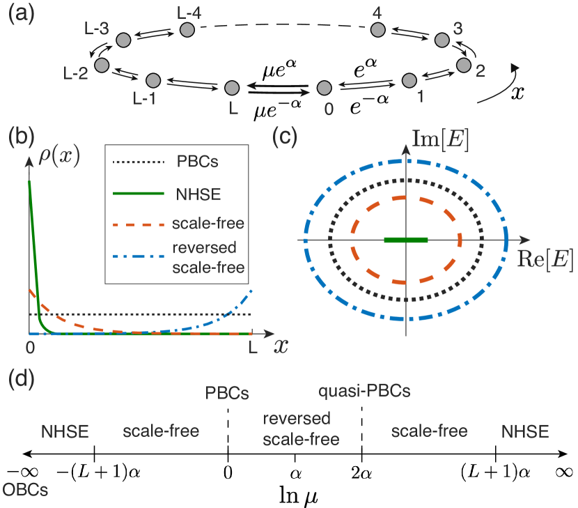
Figure 1: (a) The Hatano-Nelson model with impurity couplings $\mu e^{\pm\alpha}$. PBCs and OBCs correspond to $\mu=1$ and $0$ respectively, but other $\mu$ support qualitatively different phenomena. (b) Spatial eigenstate distributions $\rho(x)=|\psi_{x}|^{2}$ with different accumulating behaviors, with $\psi_{x}$ the wave-function value at $x$. (c) Complex spectra distinguishing the four types of eigenstates in (b). (d) Different regimes across the whole range $\mu$ are marked by different accumulation phenomena, with dualities relating strong and weak $\mu$.

Ordinary and reversed SFA. – To understand why SFA occurs, we analytically solve for the eigenstates $\Psi_{n}=\sum_{x}^{L}\psi_{x,n}\hat{c}^{\dagger}_{x}|0\rangle$, $n=0,...,L$ via $H\Psi_{n}=E_{n}\Psi_{n}$, under reasonable approximations. In the large-$\mu$ limit with $\mu\gg e^{\pm\alpha}$, two isolated eigenstates strongly localize at $x=0,L$, with eigenenergies $E_{\rm iso}\approx\pm\mu$ Sup . The other eigenstates are exponentially decaying:

$$\psi_{x,n}=e^{-\left[\kappa_{L}-i\frac{(2n+1)\pi}{L-1}\right](x-1)},x\neq 0,\kappa_{L}=\frac{\ln\mu-2\alpha}{L-1}$$ (1)

with $\psi_{0,n}\approx 0$ Sup , $n=1,2,...,L-1$ yielding $L-1$ different eigenstates. Physically, the vanishing amplitude at $x=0$ can be partially appreciated by the physics underlying electromagnetic field induced transparency Fleischhauer et al. (2005). That is, the much stronger coupling between sites $L$ and $0$ effectively makes the rest of the lattice more “transparent”, and hence suppresses the population pumping from the rest of the lattice to site 0 Sup . In a more restricted parameter regime with $e^{\alpha}\gg e^{-\alpha}$ and $\mu\ll e^{\alpha(L+1)}$, the corresponding eigenenergies can be further approximated by

$$E_{n}\approx\epsilon(k_{n}+i\kappa_{L})$$ (2)

with $k_{n}:=(2n+1)\pi/(L-1)$ and $\epsilon(k)$ the eigenenergy function at $\mu=1$ (i.e. PBCs) Sup . Remarkably, the spectrum is obtainable via a complex deformation of the PBC quasi-momentum, similar to the GBZ approach for OBC systems Yao and Wang (2018); Yokomizo and Murakami (2019); Lee and Thomale (2019). Yet, the $1/(L-1)$ coefficient in the decay exponent $\kappa_{L}$ indicates much weaker accumulation for a large system, and in fact suggests a scale-free decay profile from $x=1$ to $L$. The dependence of $\kappa_{L}$ on $\mu$ (and $L$) differs from that of impurity-induced topological localization Sup .

Counter-intuitively, reversed accumulation with negative $\kappa_{L}$ can occur when $\mu<e^{2\alpha}$, which still falls into a valid sub-regime if $\mu\gg e^{\alpha}\gg e^{-\alpha}$, as confirmed by the agreement between our approximate solutions and numerical results in Fig. 2(a). For the peculiar borderline case of $\mu=e^{2\alpha}$ between ordinary and reversed SFA, $\kappa_{L}=0$ and the eigenstates are uniformly distributed (except at $x=0$) and hence resemble Bloch states [Eq. 1 and Fig. 2(a)], even though translational invariance is broken. Indeed, the continuous part of the associated spectrum also coincides with the PBC spectrum [Eq. 2 and Fig 2(b)]. This curious case of quasi-PBC delocalized states is elaborated in the Supplemental Materials Sup . While we have considered a strong non-reciprocity of $\alpha=4$ in Fig. 2 for a better illustration, more examples with weaker $\alpha$ are found in Sup .

Figure 2: (a) Average distribution of all the anomalously accumulating eigenstates $\bar{\rho}(x)=\sum_{n=1}^{L-1}\rho_{n}(x)/(L-1)$ with $\rho_{n}(x)=|\psi_{x,n}|^{2}$ and $\alpha=4$, $L=20$. The blue, red and green cases correspond to reversed SFA, quasi-PBCs and SFA. (b) Spectra for these anomalously accumulating eigenstates, excluding the two isolated eigenstates. The black dashed curve is the true PBC spectrum ($\mu=1$), which overlaps with the quasi-PBC red curve at $\mu=e^{2\alpha}=e^{8}$. In both panels, the circles, squares, and triangles are numerical data points, and the colored solid curves are approximations from Eqs. (1),(2).

Duality between strong and weak impurity couplings.– the discussions above imply a duality between PBCs at $\mu=1$ and quasi-PBCs at $\mu=e^{2\alpha}$. This motivates us to seek duality relations for the whole range of $\mu$. For $e^{-2\alpha}\ll\mu\ll 1$, another set of exponentially decaying eigenfunctions are found, i.e.,

$$\psi^{\prime}_{x,n}=e^{-\left[\kappa_{L}^{\prime}-i\frac{2n\pi}{L+1}\right]x},\kappa_{L}^{\prime}=\frac{-\ln\mu}{L+1},$$ (3)

with

$$E^{\prime}_{n}\approx e^{\alpha}e^{\left[\ln\mu+i2n\pi\right]/(L+1)}\approx\epsilon(k_{n}^{\prime}+i\kappa_{L}^{\prime}),$$ (4)

provided that $e^{\alpha}\gg e^{-\alpha}$, where $k_{n}^{\prime}:=2n\pi/(L+1)$ Sup . Taking $\kappa_{L}$ and $\kappa_{L}^{\prime}$ as functions of $\mu$, we have $\kappa_{L}(\mu)\approx\kappa_{L}^{\prime}(e^{2\alpha}/\mu)$ for a sufficiently large system, suggesting a duality between $\mu=\mu_{\alpha}^{\pm}$ with $\mu_{\alpha}^{\pm}=e^{\alpha}A^{\pm 1}$ parametrized by a variable $A$, with $\mu_{\alpha}^{+}=\mu_{\alpha}^{-}$ at $A=1$.

This duality can be seen in both the spectrum and the eigenstate accumulation, which can be characterized by the inverse participation ratio (IPR) defined as $I_{n}=\sum_{x}|\psi_{x,n}|^{4}$ for a given eigenstate. The IPR approaches $1$ for a perfectly localized state, and $1/(L+1)$ for a spatially homogeneous one. To further characterize the different directions of the SFA states, we define a directed IPR as $I_{d,n}=\sum_{x}(x_{c}-x)|\psi_{x,n}|^{4}/(L/2)$, with $x_{c}=L/2$ being the center of the system. By definition, $I_{d}$ takes positive (negative) values for states accumulating at $x=0$ ($x=L$), and $I_{d}=0$ for a spatially homogeneous state.

In Fig. 3(a), we take averages over all continuous states for the IPRs and directed IPRs ($\bar{I}(\mu_{\alpha}^{\pm})$ and $\bar{I}_{d}(\mu_{\alpha}^{\pm})$), and present them as functions of $A$. Note that for $\mu\gg 1$, the continuous eigenstates have vanishing amplitude at $x=0$, analogous to a system with $L$, not $L+1$ sites. Therefore, to properly compare the averaged IPRs between large and small $\mu$, they are rescaled as $(\bar{I},\bar{I}_{d})\rightarrow(\bar{I},\bar{I}_{d})L/(L+1)$ for $\mu>e^{\alpha}$, and the system’s center is redefined as $x_{c}=(L-1)/2$ for the directed IPR. We can see from Fig. 3(a) that the quasi-PBCs and PBCs are recovered at $A=e^{\alpha}$ for $\mu=\mu_{\alpha}^{\pm}$ respectively, where $\bar{I}(\mu)=1/(L+1)$ and $\bar{I}_{d}(\mu)=0$ as all eigenstates are fully delocalized. The IPR profiles agree well between the dual values of $\mu$ in the regime close to PBCs and quasi-PBCs ($A\sim e^{\alpha}$), but begin to diverge when $A$ gets larger.

To understand this divergence, we unveil a second duality between $\mu\sim e^{(L+1)\alpha}$ and $\mu\sim e^{-(L+1)\alpha}$, the latter corresponds to a transition between the qualitative spectral properties found for PBCs (loops) and OBCs (lines) Koch and Budich (2020). In Fig. 3(b), we illustrate both IPRs for $\mu=\mu_{0}^{\pm}$ as functions of the variable $A$, i.e. $\mu_{0}^{\pm}=A^{\pm 1}$. The above PBC-OBC transition is seen as $\bar{I}(\mu_{0}^{-})$ and $\bar{I}_{d}(\mu_{0}^{-})$ become constant for $\ln A\geqslant(L+1)\alpha$, reflecting the OBC skin modes. Interestingly, a similar transition also occurs at large $\mu=e^{(L+1)\alpha}$, characterized by the constant IPRs in Fig. 3(b) when $\mu$ exceeds the critical value, indicating a second duality between $\mu=\mu_{0}^{\pm}$ in the large $A$ limit. These IPRs take different saturation values mainly because of the rescaling in the large $\mu$ regime with effectively different number of sites. The critical value for this transition can also be identified from our approximation of Eq. (1), where the decay exponent $\kappa_{L}=\alpha$ at $\mu=e^{(L+1)\alpha}$, recovering the decay exponent (and the imaginary flux) $\kappa_{\rm OBC}$ for NHSE under OBCs. In Fig. 3(c), we illustrate the spectra with several pairs of dual parameters, clearly showing the two types of dualities and the transition to a OBC-like spectrum.

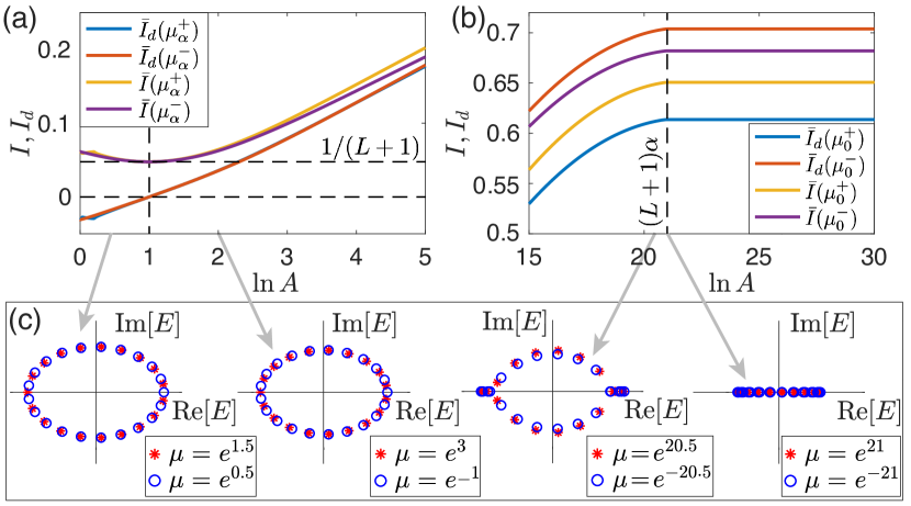
Figure 3: (a) and (b) Average IPRs defined as $\bar{I}(\mu)=\sum_{n}I_{n}/N$ and $\bar{I}_{d}(\mu)=\sum_{n}I_{n,d}/N$. The summation of $n$ runs over all continuous eigenstates, and $N=L-1$ ($L+1$) is their total number in the presence (absence) of the pair of isolated states $E_{\rm iso}\approx\pm\mu$. Colors of the curves indicate IPRs for different choices of $\mu$. Blue and red curves are almost identical in (a). (c) Spectra with dual parameters, as indicated by the gray arrows. A phase transition to OBC-like line-spectrum at $\mu=e^{\pm(L+1)\alpha}=e^{\pm 21}$, with the parameters $L=20$ and $\alpha=1$.

Co-existence of different regimes.– The decay exponents $\kappa_{L}(\mu)$ of SFA states, as induced by the impurity, are insensitive to the exact configuration of non-reciprocal hoppings in the bulk. By contrast, skin modes under OBCs may have $k$-dependent decay exponents $\kappa_{\rm OBC}(k)$ if the system has hoppings beyond nearest neighbors Lee et al. . Requiring $\kappa_{L}(\mu_{c})=\kappa_{\rm OBC}(k)$, one finds a $k$-dependent critical value of $\mu_{c}(k)$, with an intriguing consequence, namely, the co-existence of the SFA and NHSE for different eigenstates at a fixed $\mu$. Physically, this coexistence arises because at different wavenumbers $k$, an eigenstate effectively experiences couplings across different distances.

Consider a system with different forward and backward couplings ranges and an impurity between $x=0$ and $L$:

$$H_{\rm NNN}=\sum_{x=0}^{L-1}e^{\alpha}\hat{c}^{\dagger}_{x}\hat{c}_{x+1}+\mu e^{\alpha}\hat{c}^{\dagger}_{L}\hat{c}_{0}+\sum_{x=0}^{L}e^{-\alpha}\hat{c}^{\dagger}_{x}\hat{c}_{x-2}.$$ (5)

The decay exponents for the SFA at $\mu\ll 1$ and the NHSE at $\mu=0$ can be obtained as Sup ; Lee et al.

$$\kappa_{L}(\mu)=\frac{-\ln\mu}{L+1},~{}\kappa_{\rm OBC}(k)=\frac{1}{3}\ln\left[\frac{e^{2\alpha}}{2\cos(k-2j\pi/3)}\right],$$

with $j=\lfloor(k+\pi/3)/(2\pi/3)\rfloor$. In Fig. 4(a)-(c) we illustrate these two quantities versus $k$ for different $\mu$. Together with the spectra in Fig. 4(d)-(f), we see that an eigenstate always obeys the localization behavior with the smaller decaying exponent. That is, all eigenstates exhibit the SFA when $\kappa_{L}<\kappa_{\rm OBC}(k)$ in Fig. 4(a) and (d), and the NHSE when $\kappa_{L}>\kappa_{\rm OBC}(k)$ in Fig. 4(c) and (f). In the intermediate regime of Fig. 4(b) and (e), the SFA and NHSE co-exist for different $k$, as the spectrum follows the prediction of SFA when $k\in[k_{2m-1},k_{2m}]$ ($m=1,2,3$) where $\kappa_{L}$ is smaller, and the prediction of the NHSE otherwise, with $k_{2m}$ and $k_{2m-1}$ being the six special momentum values marked on Fig. 4(b) for which $\kappa_{L}=\kappa_{\rm OBC}$. As also seen from Fig. 4, due to the possibility of coexistence of the SFA and NHSE accumulation, even the qualitative spectral features are extremely sensitive to boundary impurity parameter $\mu$, an observation of general interest when it comes to build a sensing platform based on non-Hermiticity.

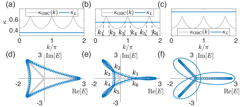
Figure 4: (a)-(c) Decaying exponents $\kappa_{L}$ and $\kappa_{\rm OBC}(k)$ of the SFA and NHSE respectively, for the Hamiltonian of Eq. (5) with different boundary impurities $\mu$. (d)-(f) Their corresponding spectra under different parameters and different boundary conditions. The blue lines, blue circles, and gray dots in (d)-(f) correspond to the spectra of the SFA where $E=\epsilon(k+i\kappa_{L})$, numerical results with a boundary impurity, and the NHSE where $E=\epsilon(k+i\kappa_{\rm OBC}(k))$ respectively, with $\epsilon(k)$ the eigenenergy under PBCs. The parameters are $\alpha=1$, $L=80$, and $\mu=10^{-30}$, $10^{-45}$, and $10^{-60}$ from left to right.

Proposed experimental demonstration.– As steady-state phenomena, the SFA can be most easily demonstrated in an electrical circuit setting. In place of the Hamiltonian, we consider the circuit Laplacian $J$ which governs its steady state response via $\mathbb{I}=J\mathbb{V}$, where the components of $\mathbb{V}$ and $\mathbb{I}$ are respectively the electrical potentials and input currents at each node. The eigenspectra and eigenstates of $J$ can be directly resolved by measuring the voltage profile Lee et al. (2018b); Helbig et al. (2019) viz.

$$V_{\alpha}=J^{-1}_{\alpha\beta}I_{\beta}=\sum_{\lambda}\frac{\langle\alpha|\psi^{R}_{\lambda}\rangle\langle\psi^{L}_{\lambda}|\mathbb{I}\rangle}{\epsilon_{\lambda}}$$ (6)

where $|\psi^{L/R}_{\lambda}\rangle$ are the left/right eigenvectors of $J$ corresponding to eigenvalue $\epsilon_{\lambda}$, and $V_{\alpha}$, $\langle\alpha|\psi^{R}_{\lambda}\rangle$ are respectively the potential and $\psi^{R}_{\lambda}$ values at the $\alpha$-th node.

To isolate a particular $\lambda^{\prime}$-th eigenmode, we tune the circuit until $\epsilon_{\lambda^{\prime}}\approx 0$, either by adjusting its variable components or by varying the AC frequency $\omega$ Lee et al. (2018b). $V_{\alpha}$ is then dominated by $\epsilon_{\lambda^{\prime}}^{-1}\langle\alpha|\psi^{R}_{\lambda^{\prime}}\rangle\langle\psi^{L}_{\lambda^{\prime}}|\mathbb{I}\rangle$. If we further connect an input current $I_{0}$ to a fixed node $\beta^{\prime}$ (the current leaves via the ground), $\langle\psi^{L}_{\lambda^{\prime}}|\mathbb{I}\rangle=I_{0}\langle\beta^{\prime}|\psi^{L}_{\lambda^{\prime}}\rangle^{*}$ and the eigenstate profile $\langle\alpha|\psi^{R}_{\lambda^{\prime}}\rangle$ across all nodes $\alpha$ becomes approximately proportional to the measured potential profile $V_{\alpha}$ i.e.

$$\psi^{R}_{\lambda^{\prime}}\approx\frac{\epsilon_{\lambda^{\prime}}\mathbb{V}}{I_{0}\langle\beta^{\prime}|\psi^{L}_{\lambda^{\prime}}\rangle^{*}}\propto\mathbb{V}.$$ (7)

In other words, $\psi_{\lambda^{\prime}}^{R}$ can be approximately measured through $\mathbb{V}$ when it is topolectrically resonant ($\epsilon_{\lambda^{\prime}}\approx 0$).

A circuit Laplacian $J$ with a similar form as $H$ of Eq. 1 can be realized with the $L+1$-node LC circuit of Fig. 5a. Adjacent nodes acquire asymmetric non-Hermitian couplings through an INIC Hofmann et al. (2019); Helbig et al. (2020) in series with a capacitor $C_{1}$, which together contribute an admittance of $i\omega C_{1}\left(\begin{matrix}-1&1\\ -1&1\end{matrix}\right)$ to the Laplacian Hofmann et al. (2019); Sup . The extent of asymmetry is regulated by another parallel capacitor $C_{2}$, such that $C_{1}/C_{2}=\tanh\alpha$ Sup . To implement an “impurity” coupling between nodes $L$ and $0$, we connect an extra variable inductor $l$ in series with the parallel INIC $+$ capacitors configuration, such that the admittance in both directions is uniformly scaled by a factor of $\mu(\omega)=\mu(\omega)=(1-\omega^{2}l(C_{2}-C_{1}))^{-1}$ Sup .

Figure 5: (a) The circuit of Eq. 8, whose asymmetric couplings are implemented through INICs and capacitors. The extra variable inductor $l$ gives rise to a coupling “impurity”. Suitably designed grounding elements Sup enable desired eigenstates to be isolated at appropriate $\omega$. (b) Simulated impedance measurements across the impurity at various $\mu$, with position $\omega$ and height of impedance peaks loosely corresponding to the real and imaginary parts of the spectrum $\epsilon/(i\omega C)$ (inset). Parameters used are $L=9$, $C_{1}=1$ and $C_{2}=3$, so that $C=\sqrt{8}$ and $\alpha=0.364$. (c) Simulated electrical potential measurements vs. the profile of the bulk eigenstate with largest $\epsilon/(i\omega C)$, tuned close to resonance via Eq. 2. Not only is Eq. 7 accurate, the nature of eigenstate accumulation also agrees perfectly with the regimes of Fig. 1d. Parameters are $L=20$, $C_{1}=2.9$, $C_{2}=3$, such that $2\alpha\approx 4$.

To measure the profile of a desired eigenmode $\psi^{R}_{\lambda^{\prime}}$, we first need to shift its eigenvalue $\epsilon_{\lambda^{\prime}}$ maximally close to $0$. This can be achieved with additional identical grounding inductors $l_{g}$ at each bulk node, together with more carefully designed grounding circuits $j_{0},j_{L}$ at the impurity nodes Sup . In all, our circuit Laplacian takes the form

$$J= \biggl{[}\mu(\omega)\left(e^{\alpha}|L\rangle\langle 0|+e^{-\alpha}|0\rangle\langle L|\right)+\sum_{x=0,\pm}^{L-1}e^{\pm\alpha}|x\rangle\langle x\pm 1|$$

$$-\sum_{x=0}^{L}\left(2\cosh\alpha-\omega_{0}^{2}/\omega^{2}\right)|x\rangle\langle x|\biggl{]}\times i\omega C$$ (8)

where $C_{1}=C\sinh\alpha$, $C_{2}=C\cosh\alpha$ and $\omega^{-2}_{0}=l_{gr}C$, which is equal to $-i\omega CH$ (Eq. 1) up to a tunable real shift (the $|x\rangle\langle x$ term). Plotted in Fig. 5b are simulated impedance measurements $Z_{0,L}=\sum_{\lambda}\epsilon_{\lambda}^{-1}\langle\Delta|\psi^{R}_{\lambda}\rangle\langle\psi_{\lambda}^{L}|\Delta\rangle$, $|\Delta\rangle=|0\rangle-|L\rangle$ Lee et al. (2018b) across the impurity as $\omega$ is varied, for different $\mu(\omega)=\mu$ adjusted through the inductors $l$. The impedance peaks correspond to values of $\omega$ where a Laplacian eigenvalue $\epsilon\approx 0$. For instance, the strongest peaks belonging to $\ln\mu=0,1$ arise from eigenvalues already on the real line (inset), while the weakest peaks from $\ln\mu=2$ are due to eigenvalues far from the real line. The entire spectrum (inset) can be reconstructed via systematic impedance measurements Helbig et al. (2019); Li et al. .

At these impedance peaks, the potential profile approximately corresponds to the eigenstate profile of the resonant eigenmode, as verified by simulated measurements [Fig 5c]. We clearly observe reversed and non-reversed eigenstates at different $\mu$, perfectly as predicted [Figs. 1d,2a]. Physically, the reversed voltage profile is a steady-state solution that represents a compromise between the competing non-reciprocal feedback mechanisms from the op-amps in the INICs. Scale-free behavior can be similarly detected when new nodes are introduced. More generally, we expect to measure these new forms of impurity-induced eigenstate accumulation in a variety of media whose steady-state description involve non-Hermitian asymmetric couplings Helbig et al. (2020); Hofmann et al. (2020); Weidemann et al. (2020).

Discussion.- Boundary impurities in a non-Hermitian non-reciprocal lattice are found to induce rich transitions between NHSE, Bloch-like and SFA eigenstates along or against the direction of non-reciprocity, with stimulating duality relations between cases of weak and strong impurity strength. Recognizing now that the well-known NHSE is only one of many impurity-induced consequences, a new basket of non-Hermitian phenomena may be explored, with the coexistence of SFA and NHSE shown as an example.

Supplementary Materials

I Derivation of circuit Laplacian

Here we provide a detailed derivation of the Laplacian (Eq. 11 of the main text) of the circuit as illustrated in Fig. 5 of the main text, and also furnish more details about its grounding connections. This circuit design is inspired by previous experimental cicuit realizations of various topological and non-Hermitian states Ningyuan et al. (2015); Lee et al. (2018b); Imhof et al. (2018); Kotwal et al. (2019); Lu et al. (2019); Olekhno et al. (2020); Lee et al. (2019b); Bao et al. (2019); Zhang et al. (2020).

The Laplacian $J$ is defined as the operator that connects the vectors of input current and electrical potential via $\mathbb{I}=J\mathbb{V}$. In this work, we design a circuit array that (i) is non-Hermitian and non-reciprocal, with right/left couplings proportional to $e^{\pm\alpha}$, (ii) has special impurity couplings (in both directions) that are stronger than the rest by a tunable factor of $\mu=\mu(\omega)$ and (iii) also contains suitable grounding elements that allows the Laplacian eigenvalue spectrum to be shifted uniformly as desired.

For (i), the unbalanced couplings $\propto e^{\pm\alpha}$ can be implemented by a parallel configuration of a capacitor $C_{2}$, and a combination of another capacitor $C_{1}$ that is connected in series with an INIC (negative impedance converter with current inversion). As elaborated in Ref. Hofmann et al. (2019), an INIC is an arrangement of operation amplifiers (op-amps) that reverses the sign of the impedance of components “in front of” it. Specifically, for a generic ideal INIC configuration as shown in Fig. S1a, the input currents and potentials at the two ends obey

$$\left(\begin{matrix}I_{A}\\ I_{B}\end{matrix}\right)=\frac{1}{Z_{A}-Z_{B}}\left(\begin{matrix}1&-1\\ 1&-1\end{matrix}\right)\left(\begin{matrix}V_{A}\\ V_{B}\end{matrix}\right)$$ (S1)

where $Z_{A},Z_{B}$ are the impedances of components A and B. The Laplacian matrix above is not just asymmetric and hence non-Hermitian, but is also inversely proportional to the difference between the two impedances, contrary to the usual case without the INIC.

To implement the $\propto e^{\pm\alpha}$ couplings, we consider parallel configurations of two capacitors $C_{1},C_{2}$, one on its own, and the other in series with an INIC (Fig. S1b). This gives a Laplacian contribution of

$$J_{\text{NN}}=i\omega C_{1}\left(\begin{matrix}1&-1\\ 1&-1\end{matrix}\right)+i\omega C_{2}\left(\begin{matrix}1&-1\\ -1&1\end{matrix}\right)=i\omega\left(\begin{matrix}C_{2}-C_{1}&C_{1}-C_{2}\\ -C_{1}-C_{2}&C_{1}+C_{2}\end{matrix}\right)=i\omega C\left(\begin{matrix}e^{-\alpha}&-e^{-\alpha}\\ -e^{\alpha}&e^{\alpha}\end{matrix}\right)$$ (S2)

if we set $C_{1}=C\sinh\alpha$, $C_{2}=C\cosh\alpha$, $C=\sqrt{C_{2}^{2}-C_{1}^{2}}$ a reference capacitance scale. If we connect each node of a OBC linear circuit array with these parallel configuration units, we end up with the Laplacian

$$J_{\text{OBC}} =i\omega\biggl{[}(C_{2}-C_{1})|0\rangle\langle 0|+(C_{2}+C_{1})|L\rangle\langle L|+\sum_{x=1}^{L-1}2C_{2}|x\rangle\langle x|-\left(\sum_{x=0}^{L-1}(C_{2}+C_{1})|x\rangle\langle x+1|+(C_{2}-C_{1})|x\rangle\langle x-1|\right)\biggl{]}$$

$$=i\omega C\biggl{[}e^{-\alpha}|0\rangle\langle 0|+e^{\alpha}|L\rangle\langle L|+\sum_{x=1}^{L-1}(2\cosh\alpha)|x\rangle\langle x|-\left(\sum_{x=0}^{L-1}e^{\alpha}|x\rangle\langle x+1|+e^{-\alpha}|x\rangle\langle x-1|\right)\biggl{]}.$$ (S3)

Note that the coefficient of $|x\rangle\langle x|$ merely sums out the total outgoing hopping amplitude.

To implement (ii) the impurity couplings that are equally asymmetric, but larger than the other couplings by a factor of $\mu$, we connect a tunable inductor $l$ with admittance $(i\omega l)^{-1}$ in series with the abovementioned parallel configuration (Fig. S1c). Elementary applications of Kirchhoff’s law gives us

$$J_{\text{imp. NN}}=i\omega\frac{(i\omega l)^{-1}}{(i\omega l)^{-1}+i\omega(C_{2}-C_{1})}\left(\begin{matrix}C_{2}-C_{1}&C_{1}-C_{2}\\ -C_{1}-C_{2}&C_{1}+C_{2}\end{matrix}\right)=\frac{1}{1-\omega^{2}(C_{2}-C_{1})l}J_{\text{NN}}=\mu(\omega)J_{\text{NN}}$$ (S4)

which is proportional to $J_{\text{NN}}$ at the two nodes coupled by the impurity, up to a factor of $\mu(\omega)=\frac{1}{1-\omega^{2}(C_{2}-C_{1})l}$. In other words, the impurity strength $\mu(\omega)$ can be adjusted both by changing the AC frequency $\omega$, or by tuning the inductor $l$ itself. Note that the upper-left term of $J_{\text{bdry. NN}}$ reduces to the simple result that the combined impedance of components connected in series is just the sum of their impedances.

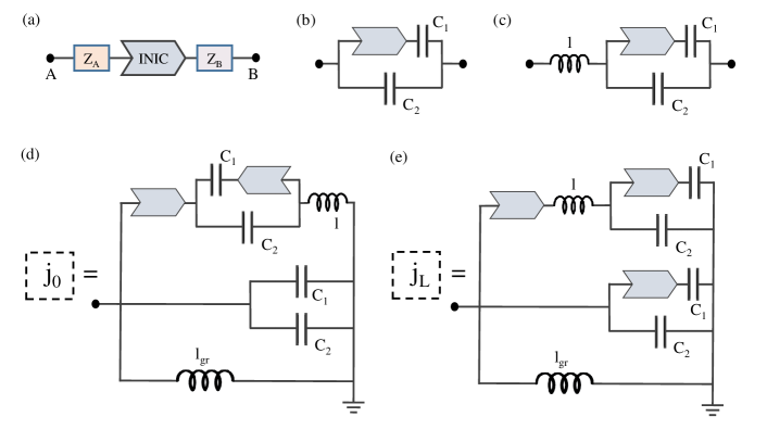
Figure S1: (a) Two generic elements with impedances $Z_{A},Z_{B}$ connected in series at either side of an INIC (elaborated in Ref. Hofmann et al. (2019)) give rise to a non-Hermitian Laplacian Eq. S1. (b) Asymmetric couplings of the simplest form (Eq. S2) can be realized with a parallel configuration containing one INIC and two capacitors. (c) An impurity bond consisting of tunable equivalently rescaled asymmetric couplings (Eq. S4) can be realized with a variable inductor $l$ connected in series with $J_{\text{NN}}$. (d,e) Explicit example realizations of $j_{0},j_{L}$ grounding components needed to make the grounding terms of the impurity nodes equivalent to the others’. Changing the AC frequency $\omega$ effects an uniform shift in Laplacian eigenvalues through $(i\omega l_{gr})^{-1}$.

The third important feature (iii), which is the implementation of grounding components that allow for a uniform shift in Laplacian eigenvalues, is more tricky. With ground connections given by $J_{\text{gr}}=\sum_{x=0}^{L}j_{x}|x\rangle\langle x|$, the circuit Laplacian we have is given by (impurity is between the $L$-th and $0$-th nodes)

$$J=J_{\text{OBC}}+J_{\text{imp. NN}}+J_{\text{gr}}=i\omega C \biggl{[}\mu(\omega)\left(e^{\alpha}|0\rangle\langle 0|+e^{-\alpha}|L\rangle\langle L|-e^{\alpha}|L\rangle\langle 0|-e^{-\alpha}|0\rangle\langle L|\right)+e^{-\alpha}|0\rangle\langle 0|+e^{\alpha}|L\rangle\langle L|$$

$$+\sum_{x=1}^{L-1}(2\cosh\alpha)|x\rangle\langle x|-\left(\sum_{x=0}^{L-1}e^{\alpha}|x\rangle\langle x+1|+e^{-\alpha}|x\rangle\langle x-1|\right)\biggl{]}+\sum_{x=0}^{L}j_{x}|x\rangle\langle x|.$$ (S5)

Notably, the on-site terms are not even uniform. For identification with the Hatano-Nelson model with a single coupling impurity (Eq. 1 of the main text), we need to add adding grounding terms such that they are not just uniform but also tunable i.e. giving rise to a tunable multiple of the $(L+1)$-by-$(L+1)$ identity matrix. Since nodes $1$ through $L-1$ already have the same onsite coefficient of $2i\omega C\cosh\alpha$, we just need to ground them via identical inductors $l_{\text{gr}}$, such that $j_{x}=(i\omega l_{\text{gr}})^{-1}$ for $x=1,...,L-1$. The more tricky part is grounding nodes $0$ and $L$ with appropriate sets of components with combined admittance $j_{0},j_{L}$ such that all onsite terms are equal. We first tidy up Eq. S5 such that the NN couplings, bulk groundings and impurity groundings are grouped together:

$$J= i\omega C\biggl{[}-\mu(\omega)\left(e^{\alpha}|L\rangle\langle 0|+e^{-\alpha}|0\rangle\langle L|\right)-\left(\sum_{x=0}^{L-1}e^{\alpha}|x\rangle\langle x+1|+e^{-\alpha}|x\rangle\langle x-1|\right)\biggl{]}+\sum_{x=1}^{L-1}\left(2i\omega C_{2}+(i\omega l_{\text{gr}})^{-1}\right)|x\rangle\langle x|$$

$$+\left[i\omega\mu(\omega)(C_{2}+C_{1})+i\omega(C_{2}-C_{1})+j_{0}\right]|0\rangle\langle 0|+\left[i\omega\mu(\omega)(C_{2}-C_{1})+i\omega(C_{2}+C_{1})+j_{L}\right]|L\rangle\langle L|.$$ (S6)

For all onsite terms to be equal, we hence require that

$$j_{0}=(i\omega l_{\text{gr}})^{-1}+i\omega(1-\mu(\omega))(C_{2}+C_{1}),$$ (S7)

$$j_{L}=(i\omega l_{\text{gr}})^{-1}+i\omega(1-\mu(\omega))(C_{2}-C_{1}).$$ (S8)

Recall from Eq. S4 that $i\omega\mu(\omega)(C_{2}\pm C_{1})$ are the admittances of the $J_{\text{imp. NN}}$ configuration with respect to the ground. The remaining admittances $i\omega(C_{2}\pm C_{1})$ can be realized by the configuration of $J_{NN}$ (Eq. S2). As such, $j_{0}$ and $j_{L}$ can be realized by the configurations illustrated in Figs. S1d and e.

All in all, our circuit Laplacian takes the form

$$J= i\omega C\biggl{[}-\mu(\omega)\left(e^{\alpha}|L\rangle\langle 0|+e^{-\alpha}|0\rangle\langle L|\right)-\left(\sum_{x=0}^{L-1}e^{\alpha}|x\rangle\langle x+1|+e^{-\alpha}|x\rangle\langle x-1|\right)\biggl{]}+\sum_{x=0}^{L}\left(2i\omega C_{2}+(i\omega l_{\text{gr}})^{-1}\right)|x\rangle\langle x|$$ (S9)

whose realization is illustrated in Fig. 5 of the main text.

II Scale-free accumulation in the Hatano-Nelson model with a boundary impurity

II.1 Strong impurity

We consider the following Hamiltonian

$$H = \sum_{x=0}^{L-1}e^{\alpha}\hat{c}^{\dagger}_{x}\hat{c}_{x+1}+e^{-\alpha}\hat{c}^{\dagger}_{x}\hat{c}_{x-1}$$ (S10)

$$+\mu_{+}\hat{c}^{\dagger}_{L}\hat{c}_{0}+\mu_{-}\hat{c}^{\dagger}_{0}\hat{c}_{L}.$$

Solving eigen-equation $H\Psi_{n}=E_{n}\Psi_{n}$ with $\Psi_{n}=\sum_{x}^{L}\psi_{x,n}\hat{c}^{\dagger}_{x}|0\rangle$ the $n$th eigenstate of the system, we obtain the following recursive conditions

$$e^{\alpha}\psi_{x+1,n}+e^{-\alpha}\psi_{x-1,n} = E_{n}\psi_{x,n}$$ (S11)

for $x=1,2,...,L-1$, and

$$\mu e^{\alpha}\psi_{0,n}+e^{-\alpha}\psi_{L-1,n} = E_{n}\psi_{L,n},$$ (S12)

$$e^{\alpha}\psi_{1,n}+\mu e^{-\alpha}\psi_{L,n} = E_{n}\psi_{0,n}.$$ (S13)

Intuitively, when $\mu$ is large, two isolated solutions localized around $x=0$ and $x=L$ are expected due to the strong couplings between these two sites. Assuming these solutions decay exponentially from the two sites into the bulk, we find that they can be explicitly expressed as

$$\psi_{0}^{+}=\psi_{L}^{+}e^{-\alpha},~{}\psi_{x}^{+}=\frac{e^{-\alpha}}{\mu}\psi_{x-1}^{+}~{}{\rm for}~{}x=1,2,...,~{}\psi_{x}^{+}=\frac{e^{\alpha}}{\mu}\psi_{x+1}^{+}~{}{\rm for}~{}x=L,L-1,...;$$ (S14)

$$\psi_{0}^{-}=-\psi_{L}^{-}e^{-\alpha},~{}\psi_{x}^{-}=-\frac{e^{-\alpha}}{\mu}\psi_{x-1}^{-}~{}{\rm for}~{}x=1,2,...,~{}\psi_{x}^{-}=-\frac{e^{\alpha}}{\mu}\psi_{x+1}^{-}~{}{\rm for}~{}x=L,L-1,...,$$ (S15)

whose eigenenergies are given by

$$E^{\pm}_{\rm iso}=\pm(\mu+\frac{1}{\mu}).$$ (S16)

These solutions are valid providing $\mu>e^{\pm\alpha}$, so that they indeed decay from $x=0$ and $x=L$ into the bulk; and $(e^{\pm\alpha}/\mu)^{L}\sim 0$, so that they have vanishing amplitudes in the middle of the system. In the main text, we have assumed $\mu\gg e^{\pm\alpha}$, therefore the above conditions are satisfied and we have $E^{\pm}_{\rm iso}\approx\pm\mu$.

For convenience, we label these two isolated eigenstates with $n=0$ and $n=L$ respectively. The other $L-1$ eigenstates of $n\in[1,L-1]$, referred as continuous eigenstates as they have a continuous spectrum, shall mainly distribute within the rest $L-1$ sites of the system with eigenenergies $E_{n}\ll\mu$, thus we shall have a vanishing $\psi_{0,n}$ from Eq. (S12). We further consider an ansatz of exponentially decaying eigenstates given by

$$\psi_{0,n}\ll 1,~{}\psi_{x,n}=e^{-M_{n}(x-1)}~{}{\rm for}~{}x\neq 0.$$ (S17)

Substituting the ansatz into Eq. (S13), we obtain

$$-e^{\alpha}=\mu e^{-\alpha}e^{-M_{n}(L-1)},$$

yielding

$$M_{n}=\frac{\ln\mu-2\alpha-i(2n+1)\pi}{L-1}:=\kappa_{L}-\frac{i(2n+1)\pi}{L-1}.$$ (S18)

However, Eqs. (S11) and (S12) give different eigenenergies with this exponentially decaying solution. A consistent solution can be obtained by further requiring $e^{\alpha}\gg e^{-\alpha}$ and $e^{\alpha}e^{-M_{n}}\gg e^{-\alpha}e^{M_{n}}$. The first condition corresponds to a strong non-reciprocity of the system, and the second one is equivalent to $\mu\ll e^{(L+1)\alpha}$, which is generally satisfied for a large enough system. Under these conditions, Eq. (S11) gives

$$E_{n}\approx e^{\alpha}e^{-M_{n}}=e^{\alpha}e^{-\left[\ln\mu-2\alpha-i(2n+1)\pi\right]/(L-1)}\approx\epsilon(k_{n}+i\kappa_{L}),$$ (S19)

with $k_{n}:=(2n+1)\pi/(L-1)$, $n=1,2,...,L-1$, and $\epsilon(k)\approx e^{\alpha}e^{ik}$ the eigenenergies under PBCs and the strong non-reciprocity. On the other hand, since now we have $\mu\gg e^{\alpha}\sim E_{n}\gg e^{-\alpha}$, the second term of Eq. (S12) can be neglected, yielding

$$|\psi_{0,n}|\approx|\frac{e^{-M_{n}L}}{\mu}|\approx\frac{e^{2\alpha}}{2\mu}\ll 1,$$ (S20)

in consistent with the vanishing $\psi_{0,n}$ obtained previously.

In Fig. S2, we compare numerical results under several different parameter regimes with the above approximation, which works well when $\mu\gg e^{\alpha}$, and $e^{\alpha}\gg e^{-\alpha}$, and $\mu\ll e^{(L+1)\alpha}$ [Fig. S2(a) and (d)]. In most other parameter regimes, while the eigenenergies and distribution of individual eigenstates cannot be predicted accurately, the average distribution of all continuous eigenstates is still in good consistence with Eqs. (S17) and (S18), as shown in the middle and right columns of Fig. S2. On the other hand, when $\mu$ approach the value of $e^{(L+1)\alpha}$, the system goes into the OBCs-like regime with the NHSE, and our approximation of the SFA is no longer valid, as discussed in the main text.

Figure S2: (a)-(c) Spatial distribution of continuous eigenstates and their (d)-(f) eigenenergies of the model of Eq. (S10). The distribution is defined as $\rho_{n}(x)=|\psi_{x,n}|^{2}$ and $\bar{\rho}(x)=\sum_{n}\rho_{n}(x)/(L-1)$. Red dashed lines indicate analytical results from the approximation. Parameters are $L=40$, and (a)(d) $\alpha=2$, $\mu=e^{1}0$; (b)(e) $\alpha=2$, $\mu=e^{2}$; and (c)(f) $\alpha=1$, $\mu=e^{1}0$.

II.2 Weak impurity

Next we consider a weak impurity limit with $\mu\ll 1$ and a strong non-reciprocity $e^{\alpha}\gg e^{-\alpha}$, and another ansatz

$$\psi^{\prime}_{x,n}=e^{-M^{\prime}_{n}x}.$$ (S21)

with $M_{n}>0$, as we observe no reversed accumulation in the regime with $\mu<1$. Thus Eq. (S13) is simplified as

$$e^{\alpha}e^{-M^{\prime}_{n}}=E^{\prime}_{n}.$$ (S22)

Substituting the above equation to Eq. (S12) with its second term being neglected, one can obtain

$$M^{\prime}_{n}=\frac{-\ln\mu-i2n\pi}{L+1}:=\kappa_{L}^{\prime}-\frac{i2n\pi}{L+1}.$$ (S23)

This solution also confirms that the second term of Eq. (S12) is neglectable comparing to the rest two terms. The eigenenergies are thus directly given by Eq. (S22).

III Quasi-PBC delocalized eigenstates

To gain further insights into the quasi-PBCs at $\mu=2\alpha$, let us exploit the following effective translational invariant Hamiltonian, $\bar{H}_{\rm PBC}(k)=H_{\rm PBC}(k+i\kappa_{L})$, with its real-space form reads as

$$\bar{H}_{\rm PBC} = \sum_{x=0}^{L}e^{-\kappa_{L}}e^{\alpha}\hat{c}^{\dagger}_{x}\hat{c}_{x+1}+e^{\kappa_{L}}e^{-\alpha}\hat{c}^{\dagger}_{x}\hat{c}_{x-1}.$$ (S24)

In above site $L+1$ is understood as site 0. According to our spectral results in Eq. 2 in the main text, $\bar{H}_{\rm PBC}$, though having an extra $\kappa_{L}$ related imaginary flux, yields the approximate eigenvalues of our lattice system for $\mu=e^{(L-1)\kappa_{L}+2\alpha}$. We next remove the imaginary flux in the bulk by applying a similarity transformation $\bar{H}_{\rm PBC}^{\prime}=S_{L}^{-1}\bar{H}_{\rm PBC}S_{L}$ with $S_{L}={\rm Diag}\{1,e^{\kappa_{L}},e^{2\kappa_{L}},...,e^{\kappa_{L}L}\}$. This gives (without changing the eigenvalues)

$$\bar{H}_{\rm PBC}^{\prime} = \sum_{x=0}^{L-1}e^{\alpha}\hat{c}^{\dagger}_{x}\hat{c}_{x+1}+e^{-\alpha}\hat{c}^{\dagger}_{x}\hat{c}_{x-1}$$ (S25)

$$+e^{-\kappa_{L}(L+1)}e^{\alpha}\hat{c}^{\dagger}_{L}\hat{c}_{0}+e^{\kappa_{L}(L+1)}e^{-\alpha}\hat{c}^{\dagger}_{0}\hat{c}_{L}.$$

So long as $L$ is sufficently large, we still have $\kappa_{L}(L+1)\approx\ln\mu-2\alpha$, thus the boundary hopping in $\bar{H}_{\rm PBC}^{\prime}$ shown above becomes

$$\mu^{-1}e^{3\alpha}\hat{c}^{\dagger}_{L}\hat{c}_{0}+\mu e^{-3\alpha}\hat{c}^{\dagger}_{0}\hat{c}_{L}.$$ (S26)

It is seen that at $\mu=e^{2\alpha}$, $\bar{H}_{\rm PBC}^{\prime}$ recovers the original Hamiltonian under PBCs. This is fully consistent with the observation from Eq. 1 in the main text, namely, the decay exponent $\kappa_{L}=0$ for $\mu=e^{2\alpha}$. The above treatment is however more stimulating to digest situations with $\mu\neq e^{2\alpha}$, where the translational invariance of $\bar{H}_{\rm PBC}^{\prime}$ is broken at the boundary. For $\mu>e^{2\alpha}$, the hopping from $x=L$ to $x=0$ is further enhanced whereas the opposite hopping is further suppressed (as respectively compared with the translational invariant case). The eigenstates are then expected to populate more at $x=0$. Likewise, eigenstates should accumulate more at $x=L$ when $\mu<e^{2\alpha}$, thereby exhibiting the reversed SFA.

IV Different accumulating behaviors of the model with two non-reciprocity length scales

We consider a system with nearest-neighbor backward couplings and next-nearest-neighbor forward couplings, and a local impurity between sites $x=0$ and $x=L$, described by the Hamiltonian

$$H_{\rm NNN} = \sum_{x=0}^{L-1}\left[e^{\alpha}\hat{c}^{\dagger}_{x}\hat{c}_{x+1}+\mu e^{\alpha}\hat{c}^{\dagger}_{L}\hat{c}_{0}\right]+\sum_{x=0}^{L}e^{-\alpha}\hat{c}^{\dagger}_{x}\hat{c}_{x-2}.$$ (S27)

Solve eigen-function $H_{\rm NNN}\Psi_{n}=E_{n}\Psi_{n}$ with $\Psi_{n}=\sum_{x}^{L}\psi_{x,n}\hat{c}^{\dagger}_{x}|0\rangle$, the recursive conditions of $\psi_{x,n}$ are given by

$$e^{\alpha}\psi_{x+1,n}+e^{-\alpha}\psi_{x-2,n}=E_{n}\psi_{x,n}$$ (S28)

for $x=1,2,...,L-1$, and

$$\mu e^{\alpha}\psi_{0,n}+e^{-\alpha}\psi_{L-2,n} = E_{n}\psi_{L,n},$$ (S29)

$$e^{\alpha}\psi_{1,n}+e^{-\alpha}\psi_{L-1,n} = E_{n}\psi_{0,n}.$$ (S30)

Similarly to the model of Eq. (S10) at weak impurity limit, we consider the parameter regime with $\mu\ll 1$ and $e^{\alpha}\gg e^{-\alpha}$, and the same SFA solution can be obtained as

$$\psi_{x,n}=e^{-M_{n}x},~{}M_{n}=\frac{-\ln\mu-i2n\pi}{L+1}:=\kappa_{L}-\frac{i2n\pi}{L+1}.$$ (S31)

On the other hand, to solve the OBC system with $\mu=0$, we consider the an imaginary flux $\kappa_{\rm OBC}(k)$ under PBCs, corresponding an effective Hamiltonian

$$\bar{H}_{\rm NNN}(k)=H_{\rm NNN}(k+i\kappa_{\rm OBC}(k))=ze^{\alpha}+e^{-\alpha}/z^{2},$$ (S32)

with $z=e^{i[k+i\kappa_{\rm OBC}(k)]}$. The OBC system is described by a GBZ, where the eigenenergies satisfy $\bar{E}(k_{1})=\bar{E}(k_{2})$ for pairs of quasi-momenta with $\kappa_{\rm OBC}(k_{1})=\kappa_{\rm OBC}(k_{2})$. Numerically, we find that this condition is satisfied when $k_{1}+k_{2}=0$, $2\pi/3$, and $4\pi/3$, for $k_{1},k_{2}\in[-\pi/3,\pi/3]$, $[\pi/3,\pi]$, and $[\pi,5\pi/3]$, respectively. With these relations between $k_{1}$ and $k_{2}$, we obtain

$$\kappa_{\rm OBC}(k) = \frac{1}{3}\ln\left[\frac{e^{2\alpha}}{2\cos(k-2j\pi/3)}\right],$$ (S33)

with $j=\lfloor(k+\pi/3)/(2\pi/3)\rfloor$.

V Co-existence of SFA and topological localization

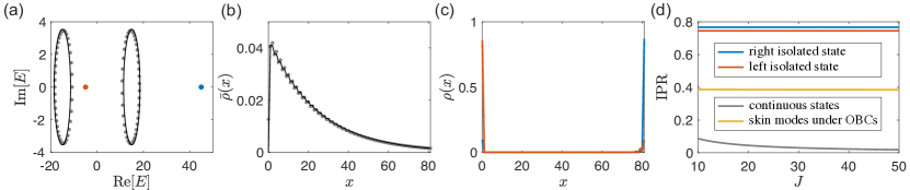
Figure S3: (a) the full spectrum of the SSH model with a local on-site potential, gray dots are the continuous states, blue and red dots are the two topological/isolated states. (b) the average distribution of the continuous states. (c) The distributions of the topological/isolated states. (4d) IPR versus system’s size for different eigenstates of the system with a local on-site potential, and for skin modes under OBCs. The results for continuous states and skin modes are the average values of all corresponding eigenstates. Parameters are $\alpha=2$, $t_{ab}=15$, $\mu=40$, and $J=40$ for (a,b,c).

In this section we consider a non-Hermitian topological system with non-reciprocal couplings, where SFA and topological localization exist for different eigenstates of the system. The explicit model we consider is a non-reciprocal Su-Schrieffer-Heeger (SSH) model Su et al. (1979), described by the Hamiltonian

$$H = \sum_{j=0}^{J}e^{\alpha}\hat{a}^{\dagger}_{j}\hat{b}_{j}+e^{-\alpha}\hat{b}^{\dagger}_{j}\hat{a}_{j}$$ (S34)

$$+t_{ab}\hat{b}^{\dagger}_{j}\hat{a}_{j+1}+h.c.+\mu\hat{b}^{\dagger}_{J}\hat{b}_{J}$$

with $J+1$ the number of unit cells. Note that instead of enhanced boundary couplings, here spatial inhomogeneity is induced by an on-site potential acting on a single lattice site, so that only one isolated state shall emerge due to the impurity, in the absence of a nontrivial topology. The existence of isolated boundary states and their connection to the bulk topology has been studied in Ref. Liu and Chen , and here we shall focus on the topologically nontrivial regime of $t_{ab}>e^{\alpha}$, with strong local potential $\mu\gg t_{ab}$. By solving the eigen-equation $H\Psi_{n}=E_{n}\Psi_{n}$ with eigenstates defined as $\Psi_{n}\sum_{j}^{J}(\psi^{a}_{j,n}\hat{a}^{\dagger}_{j,n}+\psi^{b}_{j,n}\hat{b}^{\dagger}_{j,n})|0\rangle$, we obtain the solutions

$$\psi^{b}_{j,n} = e^{-\left[\kappa_{J}-i(2n+1)\pi/J\right]j},\psi_{j,n}^{a}=\phi_{j-1,n}^{b},$$

$$\kappa_{J} \approx \left[\ln\mu-\alpha\right]/J$$ (S35)

with a continuous spectrum

$$E_{n}\approx\pm\left(t_{ab}+\frac{e^{\alpha-\kappa_{J}}e^{\left[\alpha-i(2n+1)\pi\right]/J}}{2}\right),$$ (S36)

exhibiting the same scale-free decaying behavior as in the main text, due to the $1/J$ coefficient in $\kappa_{J}$.

In the parameter regime we choose, the system holds two eigenstates isolated from the continuous spectrum, as shown in Fig. S3(a). Associated with the nontrivial bulk topology, these two states localized at $j=0$ and $j=J$ respectively [Fig. S3(b)], with the later one affected more by the local potential at $j=J$ and having an eigenenergy $E\approx\mu$. On the other hand, both of these two states exhibit a much stronger accumulation to the boundary, in contrast with the continuous states illustrated in Fig. S3(c).

To further characterize their difference, we calculate the inverse participation ratio (IPR) defined as ${\rm IPR}=\sum_{j}(|\psi^{a}_{j}|^{4}+|\psi^{b}_{j}|^{4})$ for the isolated states, continuous states, and skin modes under OBCs (with $\mu=0$), and demonstrate it versus the system’s size $J$ in Fig. S3(d). Besides their weaker accumulation reflected by a smaller IPR, the continuous states are less localized for a larger size of the system, due to the $1/J$ coefficient in the decaying exponent $\kappa_{J}$. On the other hand, the IPR for isolated states, and for the skin modes under OBCs, remains a constant when increasing the size.

References

- Yao and Wang (2018) Shunyu Yao and Zhong Wang, “Edge states and topological invariants of non-hermitian systems,” Phys. Rev. Lett. 121, 086803 (2018).
- Yokomizo and Murakami (2019) Kazuki Yokomizo and Shuichi Murakami, “Non-bloch band theory of non-hermitian systems,” Physical review letters 123, 066404 (2019).
- Lee and Thomale (2019) Ching Hua Lee and Ronny Thomale, “Anatomy of skin modes and topology in non-hermitian systems,” Phys. Rev. B 99, 201103 (2019).
- Lee et al. (2018a) Ching Hua Lee, Guangjie Li, Yuhan Liu, Tommy Tai, Ronny Thomale, and Xiao Zhang, “Tidal surface states as fingerprints of non-hermitian nodal knot metals,” arXiv preprint arXiv:1812.02011 (2018a).
- Kunst and Dwivedi (2019) Flore K Kunst and Vatsal Dwivedi, “Non-hermitian systems and topology: A transfer-matrix perspective,” Physical Review B 99, 245116 (2019).
- Edvardsson et al. (2019) Elisabet Edvardsson, Flore K Kunst, and Emil J Bergholtz, “Non-hermitian extensions of higher-order topological phases and their biorthogonal bulk-boundary correspondence,” Physical Review B 99, 081302 (2019).
- (7) Zhesen Yang, Kai Zhang, Chen Fang, and Jiangping Hu, “Auxiliary generalized brillouin zone method in non-hermitian band theory,” 1912.05499v1 .
- Zhang et al. (2019) Kai Zhang, Zhesen Yang, and Chen Fang, “Correspondence between winding numbers and skin modes in non-hermitian systems,” arXiv preprint arXiv:1910.01131 (2019).
- Brandenbourger et al. (2019) Martin Brandenbourger, Xander Locsin, Edan Lerner, and Corentin Coulais, “Non-reciprocal robotic metamaterials,” Nature communications 10, 1–8 (2019).
- Lee et al. (2019a) Ching Hua Lee, Linhu Li, and Jiangbin Gong, “Hybrid higher-order skin-topological modes in nonreciprocal systems,” Phys. Rev. Lett. 123, 016805 (2019a).
- Mu et al. (2019) Sen Mu, Ching Hua Lee, Linhu Li, and Jiangbin Gong, “Emergent fermi surface in a many-body non-hermitian fermionic chain,” arXiv preprint arXiv:1911.00023 (2019).
- Li et al. (2019) Linhu Li, Ching Hua Lee, and Jiangbin Gong, “Geometric characterization of non-hermitian topological systems through the singularity ring in pseudospin vector space,” Physical Review B 100, 075403 (2019).
- Lee and Longhi (2020) Ching Hua Lee and Stefano Longhi, “Ultrafast and anharmonic rabi oscillations between non-bloch-bands,” arXiv preprint arXiv:2003.10763 (2020).
- Longhi (2020) Stefano Longhi, “Non-bloch-band collapse and chiral zener tunneling,” Physical Review Letters 124, 066602 (2020).
- Lee (2020) Ching Hua Lee, “Many-body topological and skin states without open boundaries,” arXiv preprint arXiv:2006.01182 (2020).
- Cao et al. (2020) Yang Cao, Yang Li, and Xiaosen Yang, “Non-hermitian bulk-boundary correspondence in periodically driven system,” arXiv preprint arXiv:2007.13499 (2020).
- Xue et al. (2020) Wen-Tan Xue, Ming-Rui Li, Yu-Min Hu, Fei Song, and Zhong Wang, “Non-hermitian band theory of directional amplification,” arXiv preprint arXiv:2004.09529 (2020).
- Liu et al. (2020) Chun-Hui Liu, Kai Zhang, Zhesen Yang, and Shu Chen, “Helical damping and anomalous critical non-hermitian skin effect,” arXiv preprint arXiv:2005.02617 (2020).
- Rosa and Ruzzene (2020) Matheus IN Rosa and Massimo Ruzzene, “Dynamics and topology of non-hermitian elastic lattices with non-local feedback control interactions,” New Journal of Physics 22, 053004 (2020).
- Yoshida et al. (2020) Tsuneya Yoshida, Tomonari Mizoguchi, and Yasuhiro Hatsugai, “Mirror skin effect and its electric circuit simulation,” Physical Review Research 2, 022062 (2020).
- Yi and Yang (2020) Yifei Yi and Zhesen Yang, “Non-hermitian skin modes induced by on-site dissipations and chiral tunneling effect,” arXiv preprint arXiv:2003.02219 (2020).
- Xiao et al. (2020) Lei Xiao, Tianshu Deng, Kunkun Wang, Gaoyan Zhu, Zhong Wang, Wei Yi, and Peng Xue, “Non-hermitian bulk–boundary correspondence in quantum dynamics,” Nature Physics , 1–6 (2020).
- Li et al. (2020) Linhu Li, Ching Hua Lee, and Jiangbin Gong, “Topological switch for non-hermitian skin effect in cold-atom systems with loss,” Physical Review Letters 124, 250402 (2020).
- Schomerus (2020) Henning Schomerus, “Nonreciprocal response theory of non-hermitian mechanical metamaterials: Response phase transition from the skin effect of zero modes,” Physical Review Research 2, 013058 (2020).
- Okuma et al. (2020) Nobuyuki Okuma, Kohei Kawabata, Ken Shiozaki, and Masatoshi Sato, “Topological origin of non-hermitian skin effects,” Phys. Rev. Lett. 124, 086801 (2020).
- Koch and Budich (2020) Rebekka Koch and Jan Carl Budich, “Bulk-boundary correspondence in non-hermitian systems: stability analysis for generalized boundary conditions,” The European Physical Journal D 74, 1–10 (2020).
- Teo et al. (2020) Wei Xin Teo Teo, Linhu Li, Xizheng Zhang, and Jiangbin Gong, “Topological characterization of non-hermitian multiband systems using majorana’s stellar representation,” Physical Review B 101, 205309 (2020).
- (28) Linhu Li, Ching Hua Lee, Sen Mu, and Jiangbin Gong, “Critical non-hermitian skin effect,” 2003.03039v1 .
- Bosch et al. (2019) Martí Bosch, Simon Malzard, Martina Hentschel, and Henning Schomerus, “Non-hermitian defect states from lifetime differences,” Physical Review A 100, 063801 (2019).
- Liu and Chen (2019) Chun-Hui Liu and Shu Chen, “Topological classification of defects in non-hermitian systems,” Physical Review B 100, 144106 (2019).
- X. L. Zhao (2020) L. B. Fu X. X. Yi X. L. Zhao, L. B. Chen, “Topological phase transition of non‐hermitian crosslinked chain,” Annalen der Physik 532, 1900402 (2020).
- (32) Yanxia Liu and Shu Chen, “Diagnosis of bulk phase diagram of non-reciprocal topological lattices by impurity modes,” 2001.05688v1 .
- (33) Xi-Wang Luo and Chuanwei Zhang, “Non-hermitian disorder-induced topological insulators,” 1912.10652v1 .
- Longhi (2019) Stefano Longhi, “Topological phase transition in non-hermitian quasicrystals,” Physical Review Letters 122, 237601 (2019).
- Jiang et al. (2019) Hui Jiang, Li-Jun Lang, Chao Yang, Shi-Liang Zhu, and Shu Chen, “Interplay of non-hermitian skin effects and anderson localization in nonreciprocal quasiperiodic lattices,” Physical Review B 100, 054301 (2019).
- Zeng et al. (2020) Qi-Bo Zeng, Yan-Bin Yang, and Yong Xu, “Topological phases in non-hermitian aubry-andré-harper models,” Physical Review B 101, 020201 (2020).
- Claes and Hughes (2020) Jahan Claes and Taylor L Hughes, “Skin effect and winding number in disordered non-hermitian systems,” arXiv preprint arXiv:2007.03738 (2020).
- Xiong (2018) Ye Xiong, “Why does bulk boundary correspondence fail in some non-hermitian topological models,” Journal of Physics Communications 2, 035043 (2018).
- (39) Jan Carl Budich and Emil J. Bergholtz, “Non-hermitian topological sensors,” 2003.13699v1 .
- McDonald and Clerk (2020) Alexander McDonald and Aashish A Clerk, “Exponentially-enhanced quantum sensing with non-hermitian lattice dynamics,” arXiv preprint arXiv:2004.00585 (2020).
- Hatano and Nelson (1996) Naomichi Hatano and David R. Nelson, “Localization transitions in non-hermitian quantum mechanics,” Phys. Rev. Lett. 77, 570–573 (1996).
- (42) “Supplemental materials,” Supplemental Materials .
- Fleischhauer et al. (2005) Michael Fleischhauer, Atac Imamoglu, and Jonathan P. Marangos, “Electromagnetically induced transparency: Optics in coherent media,” Rev. Mod. Phys. 77, 633–673 (2005).
- (44) Ching Hua Lee, Linhu Li, Ronny Thomale, and Jiangbin Gong, “Unraveling non-hermitian pumping: emergent spectral singularities and anomalous responses,” 1912.06974v2 .
- Lee et al. (2018b) Ching Hua Lee, Stefan Imhof, Christian Berger, Florian Bayer, Johannes Brehm, Laurens W Molenkamp, Tobias Kiessling, and Ronny Thomale, “Topolectrical circuits,” Communications Physics 1, 1–9 (2018b).
- Helbig et al. (2019) Tobias Helbig, Tobias Hofmann, Ching Hua Lee, Ronny Thomale, Stefan Imhof, Laurens W Molenkamp, and Tobias Kiessling, “Band structure engineering and reconstruction in electric circuit networks,” Physical Review B 99, 161114 (2019).
- Hofmann et al. (2019) Tobias Hofmann, Tobias Helbig, Ching Hua Lee, Martin Greiter, and Ronny Thomale, “Chiral voltage propagation and calibration in a topolectrical chern circuit,” Physical review letters 122, 247702 (2019).
- Helbig et al. (2020) T Helbig, T Hofmann, S Imhof, M Abdelghany, T Kiessling, LW Molenkamp, CH Lee, A Szameit, M Greiter, and R Thomale, “Generalized bulk–boundary correspondence in non-hermitian topolectrical circuits,” Nature Physics , 1–4 (2020).
- Hofmann et al. (2020) Tobias Hofmann, Tobias Helbig, Frank Schindler, Nora Salgo, Marta Brzezińska, Martin Greiter, Tobias Kiessling, David Wolf, Achim Vollhardt, Anton Kabaši, et al., “Reciprocal skin effect and its realization in a topolectrical circuit,” Physical Review Research 2, 023265 (2020).
- Weidemann et al. (2020) Sebastian Weidemann, Mark Kremer, Tobias Helbig, Tobias Hofmann, Alexander Stegmaier, Martin Greiter, Ronny Thomale, and Alexander Szameit, “Efficient light funneling based on the non-hermitian skin effect,” arXiv preprint arXiv:2004.01990 (2020).
- Ningyuan et al. (2015) Jia Ningyuan, Clai Owens, Ariel Sommer, David Schuster, and Jonathan Simon, “Time-and site-resolved dynamics in a topological circuit,” Phys. Rev. X 5, 021031 (2015).
- Imhof et al. (2018) Stefan Imhof, Christian Berger, Florian Bayer, Johannes Brehm, Laurens W Molenkamp, Tobias Kiessling, Frank Schindler, Ching Hua Lee, Martin Greiter, Titus Neupert, et al., “Topolectrical-circuit realization of topological corner modes,” Nature Physics 14, 925 (2018).
- Kotwal et al. (2019) Tejas Kotwal, Henrik Ronellenfitsch, Fischer Moseley, Alexander Stegmaier, Ronny Thomale, and Jörn Dunkel, “Active topolectrical circuits,” arXiv preprint arXiv:1903.10130 (2019).
- Lu et al. (2019) Yuehui Lu, Ningyuan Jia, Lin Su, Clai Owens, Gediminas Juzeliūnas, David I Schuster, and Jonathan Simon, “Probing the berry curvature and fermi arcs of a weyl circuit,” Physical Review B 99, 020302 (2019).
- Olekhno et al. (2020) Nikita A Olekhno, Egor I Kretov, Andrei A Stepanenko, Polina A Ivanova, Vitaly V Yaroshenko, Ekaterina M Puhtina, Dmitry S Filonov, Barbara Cappello, Ladislau Matekovits, and Maxim A Gorlach, “Topological edge states of interacting photon pairs emulated in a topolectrical circuit,” Nature Communications 11, 1–8 (2020).
- Lee et al. (2019b) Ching Hua Lee, Tobias Hofmann, Tobias Helbig, Yuhan Liu, Xiao Zhang, Martin Greiter, and Ronny Thomale, “Imaging nodal knots in momentum space through topolectrical circuits,” arXiv preprint arXiv:1904.10183 (2019b).
- Bao et al. (2019) Jiacheng Bao, Deyuan Zou, Weixuan Zhang, Wenjing He, Houjun Sun, and Xiangdong Zhang, “Topoelectrical circuit octupole insulator with topologically protected corner states,” Physical Review B 100, 201406 (2019).
- Zhang et al. (2020) Weixuan Zhang, Deyuan Zou, Wenjing He, Jiacheng Bao, Qingsong Pei, Houjun Sun, and Xiangdong Zhang, “Topolectrical-circuit realization of 4d hexadecapole insulator,” arXiv preprint arXiv:2001.07931 (2020).
- Su et al. (1979) W. P. Su, J. R. Schrieffer, and A. J. Heeger, “Solitons in polyacetylene,” Phys. Rev. Lett. 42, 1698–1701 (1979).