Vanadium Abundance Derivations in 255 Metal-poor Stars

Abstract

We present vanadium (V) abundances for 255 metal-poor stars, derived from high-resolution optical spectra from the Magellan Inamori Kyocera Echelle spectrograph on the Magellan Telescopes at Las Campanas Observatory, the Robert G. Tull Coudé Spectrograph on the Harlan J. Smith Telescope at McDonald Observatory, and the High Resolution Spectrograph on the Hobby-Eberly Telescope at McDonald Observatory. We use updated V i and V ii atomic transition data from recent laboratory studies, and we increase the number of lines examined (from 1 to 4 lines of V i, and from 2 to 7 lines of V ii). As a result, we reduce the V abundance uncertainties for most stars by more than 20 % and expand the number of stars with V detections from 204 to 255. In the metallicity range $-$4.0 $<$ [Fe/H] $<-$1.0, we calculate the mean ratios [V i/Fe i] $=-0.10\pm 0.01~{}(\sigma=0.16)$ from 128 stars with $\geq$ 2 V i lines detected, [V ii/Fe ii] $=+0.13\pm 0.01~{}(\sigma=0.16)$ from 220 stars with $\geq$ 2 V ii lines detected, and [V ii/V i] $=+0.25\pm 0.01~{}(\sigma=0.15)$ from 119 stars. We suspect this offset is due to non-LTE effects, and we recommend using [V ii/Fe ii], which is enhanced relative to the solar ratio, as a better representation of [V/Fe]. We provide more extensive evidence for abundance correlations detected previously among scandium, titanium, and vanadium, and we identify no systematic effects in the analysis that can explain these correlations.

1 Introduction

Metal-poor stars in the halo record the early chemical enrichment history of the Galaxy. With only a few prior stellar explosions pouring metals into the environment, their chemical compositions tell us about the nucleosynthetic processes responsible for creating many of the heavy elements in the universe. Many theoretical supernova (SN) models have been used to provide predictions about the relative chemical abundances in these metal-poor stars.

In particular, the nucleosynthesis of iron-group elements has been studied in detail to inform Galactic chemical evolution models (e.g., Kobayashi et al. 2011; Curtis et al. 2019). In general, these elements are produced mostly in core-collapse supernovae (CCSNe) and explosive stellar yields. Specifically, scandium (Sc, $Z=21$), titanium (Ti, $Z=22$), and vanadium (V, $Z=23$) are produced by explosive silicon burning and oxygen burning in the core collapse SN phase, while the other iron-group elements are also produced by incomplete or complete silicon burning in the CCSNe ejecta (Woosley & Weaver, 1995). While significant developments in abundance derivations have been made over the past decade, challenges exist for obtaining reliable abundances for these elements. Vanadium, along with other iron-group elements (21 $\leq Z\leq$ 28), is present in the atmospheres of metal-poor stars mostly in the ionized state. These ionized-species transitions usually require blue or ultraviolet (UV) spectra for detection. They also require accurate laboratory atomic transition data to yield reliable abundances. Using accurate and precise transition probabilities and hyperfine/isotopic substructure atomic data from the Wisconsin atomic physics group, Sneden et al. (2016) derived iron-group element abundances for the very metal-poor star HD 84937. They discovered that the abundances of scandium, titanium, and vanadium were all enhanced, relative to iron (Fe, $Z=26$) in HD 84937, and they confirmed that similar correlations exist among larger samples of metal-poor stars using data from Cayrel et al. (2004), Cohen et al. (2004, 2008), Barklem et al. (2005), Lai et al. (2008), Yong et al. (2013), and Roederer et al. (2014). Recently, Cowan et al. (2020) reported iron-group abundances for three main-sequence turnoff stars with metallicities [Fe/H] $\sim-3$, confirming and extending the trends found in Sneden et al. (2016).

So far, current CCSN models cannot fully explain the correlations observed in the halo metal poor stars. Sneden et al. (2016) described the possible common production process for titanium and vanadium, but they raised questions on the theoretical reasons for the correlation between scandium and the other two elements. Not only is it unclear how the complex production history of scandium ties to its correlation with vanadium and titanium, but the abundance of scandium itself is also difficult to reproduce theoretically. Our current Galactic chemical evolution (GCE) models, in general, underestimate the abundances of scandium, titanium, and vanadium in metal-poor stars (Kobayashi et al., 2006).

It has been suggested that a 50 % hypernova fraction at early Galactic times may be able to explain the overall overabundance of these elements (Umeda & Nomoto, 2002; Kobayashi et al., 2006). Umeda & Nomoto calculated nucleosynthesis with CCSNe models and compare them with observations to constrain the parameters, with an emphasis on trying to recover the high iron-group element production. They find that deep mixing, deep mass cuts, smaller neutron excesses, and larger explosion energies produce higher iron-group abundances in general. Yet, even then scandium is still underproduced, although a better match could potentially be obtained by introducing jets and neutrino effects (Kobayashi et al., 2006, 2011). Following that direction, Curtis et al. (2019) managed to reproduce most of the abundance measurements of the very metal-poor star HD 84937, studied in Sneden et al. (2016), using CCSNe models that consistently capture the neutrino interactions, but with large variations in scandium and zinc. It is also unclear how these new CCSNe models will impact the GCE calculations, which require the inclusion of a stellar initial mass function, star formation history, and other factors. Therefore, so far, the correlations observed in samples of many metal-poor stars cannot be explained by current CCSN models.

The abundances reported in the large-sample studies comprise a heterogeneous set, with variations in stellar evolutionary states, spectral wavelength coverage, resolution, and signal-to-noise, and analytical techniques. Moreover, these abundances may not be reliable due to the lack of accurate atomic transition data. In particular, vanadium had fewer reliable transitions available for measurement prior the publication of new laboratory atomic data from Lawler et al. (2014) and Wood et al. (2014). Roederer et al. (2014) presented V i detections in 134 stars (including 16 without V ii) from 1 V i line, V ii detections in 188 stars (including 70 without V i) from 2 V ii lines, for a total of 204 stars with either V i or V ii detections. To further test the correlations found by Sneden et al. (2016), we apply the improved atomic data to rederive the vanadium abundances for stars in this sample.

In Section 2, we provide a quick review of the high-resolution spectroscopic data from Roederer et al. (2014). We discuss the analysis methods and uncertainty estimates in Section 3, where we also include the individual fitting for each transition and the calibrations applied. The new vanadium abundances and their correlations with other parameters are presented in Section 4. We discuss the significance of our results in Section 5, and we conclude in Section 6.

We adopt the standard definitions of elemental abundances and ratios. The logarithmic absolute abundance for element X is defined as the number of atoms of X per $10^{12}$ hydrogen atoms, $\log\epsilon\text{(X)}\equiv\log_{10}{(N_{X}/N_{H})}+12.0$. For elements X and Y, the logarithmic abundance ratio relative to the solar ratio is defined as [X/Y] $\equiv\log_{10}{(N_{X}/N_{Y})}-\log_{10}{(N_{X}/N_{Y})}_{\odot}$. We adopt the solar abundances of Asplund et al. (2009), where $\log\epsilon\text{(V)}=3.93$. We note that, when denoted with the ionization state (e.g., $\log\epsilon\text{(X~{}{i})}$), the value still represents the total elemental abundance, derived from transitions of that particular ionization state after applying Saha ionization corrections.

2 Observations

In this work, we adopt the same sample and spectra used in the Roederer et al. (2014) study without change. It should be noted that these targets were selected from various surveys in a highly heterogeneous manner. They are stars that are deemed to be chemically interesting and bright enough to be suitable for high resolution, high S/N spectroscopy. Thus, they do not represent an unbiased stellar population. Yet, the selection criteria do not include any constraints on the vanadium abundances of the targets, so this sample was chosen without bias to the vanadium abundances.

For most of the stars, the spectroscopy was obtained using the Magellan Telescopes at Las Campanas Observatory using the Magellan Inamori Kyocera Echelle (MIKE) spectrograph (Bernstein et al., 2003). The MIKE spectra cover wavelengths of 3350-7250 Å, with $R\sim 41,000$ and S/N $\sim 40$ per resolution element (RE) at 3950 Å.  Some observations were made with the Robert G. Tull Coudé Spectrograph (Tull et al., 1995) on the 2.7 m Harlan J. Smith Telescope at McDonald Observatory (MCD), with narrower wavelength coverage 3700-5700 Å, $R\sim 30,000$, and S/N $\sim 50$ $\text{RE}^{-1}$ at 3950 Å.  The narrower wavelength coverage at the blue end prevents us from using two useful short-wavelength V ii lines to derive abundances. The narrower wavelength coverage at the red end does not cause problems. Other observations were made with the High Resolution Spectrograph on the 9.2m Hobby-Eberly Telescope at McDonald Observatory (HET), with wavelength coverage 3900-6800 Å, $R\sim 30,000$, and S/N $\sim 20$ $\text{RE}^{-1}$ at 3950 Å.  The 3900 Å blue cutoff of the HET spectra limits the V ii transitions to four lines. Further details of the instrument setup and observing strategy may be found in Roederer et al. (2014).

In total, 250 stars were observed with MIKE, 52 with MCD, and 19 with HET.  Accounting for the repeat observations of stars and three double-lined spectroscopic binaries, which are not examined here, 313 stars are available for examination. The duplicate observations of the same stars using different instruments serves as a tool to examine consistency across instruments, which is further discussed in Section 3.4.

3 Methods

3.1 Model Atmospheres

For the model atmospheres, we adopt the same set of MARCS models (Gustafsson et al., 2008) that was used in Roederer et al. (2014). We assume 1D, plane-parallel, static model atmospheres in local thermodynamic equilibrium (LTE) throughout the line-forming layers. As described in Roederer et al., most of the model atmosphere parameters are derived from the spectra. The effective temperatures ($T_{\rm eff}$) are derived by enforcing that the iron abundances derived from the neutral lines have no trend with the excitation potential (E.P.) of the lower level of the transition. The typical statistical uncertainty in $T_{\rm eff}$ ranges from 40-50 K.  Similarly, microturbulence velocities ($v_{\rm t}$) are derived by requiring no trend with line strength. The statistical uncertainty in $v_{\rm t}$ is approximately 0.06 km s^-1. Surface gravities (log g) are derived by interpolation from $T_{\rm eff}$using theoretical isochrones in the $\text{Y}^{2}$ grid (Demarque et al., 2004), except for the horizontal branch (HB), main sequence (MS), and blue straggler-like (BS) classes, which are derived using the usual method of requiring the ionization balance between Fe i and Fe ii. The statistical uncertainty in log g ranges between 0.15 and 0.25 dex. The overall metallicity is simply the iron abundance derived from Fe ii lines. The statistical uncertainty for metallicity is approximately 0.07 dex. All uncertainties mentioned above do not include the systematic uncertainties. We adopt these derived model parameters and the associated models for the spectral synthesis in this work to derive vanadium abundances.

As discussed extensively in Roederer et al. (2014), systematic uncertainties are very difficult to quantify accurately. They can be estimated by comparing the derived stellar parameters obtained through different techniques. Roederer et al. (2014) provides systematic uncertainties of the stellar parameters for different evolutionary stages in this sample. For example, the systematic difference in log g values can be calculated from the $\text{Y}^{2}$ set of isochrones and another set in common use, the PARSEC grid (Bressan et al., 2012). For metal-poor red giants, the difference in log g at fixed $T_{\rm eff}$ is $\approx$ 0.2–0.3 dex, with the $\text{Y}^{2}$ set of models giving larger log g values. For metal-poor subgiants, the difference is even smaller, $<$ 0.1 dex, and the two sets of isochrones yield nearly identical results around 6000 K. These systematic differences are comparable to the 1$\sigma$ statistical uncertainties in the log g values, and they would affect all stars of similar $T_{\rm eff}$ equally. Such changes have minimal impact on the derived [V/Fe] ratios. (Section 4.1). For our purpose, which is to compare abundances ratios of stars within the sample itself, it is sufficient to just consider the statistical uncertainties. Furthermore, when we discuss the correlation of vanadium abundances with other iron-group elements in Section 4.3, the abundance ratios of those elements are also derived based on the same models.

3.2 Abundance Analysis

We derive the vanadium abundances using synthetic spectra generated with the LTE line analysis code MOOG (Sneden, 1973; Sobeck et al., 2011). The analysis code produces synthetic spectra sets based on different assumptions on vanadium abundance of each star. We then obtain the vanadium abundance for each star by iterative comparison of the synthetic spectra to the observed spectrum. Line lists used for the syntheses, including the new laboratory transition data for both V i (Lawler et al., 2014) and V ii (Wood et al., 2014), are listed in Table 1. We start with 6 V i and 20 V ii lines that are available in the wavelength range of our spectra. We generate test syntheses for all 26 lines in stars ranging from metal-poor subgiants (CS 22886–012) to metal-rich red giants (HD 21581). We identify 4 V i and 7 V ii lines that are relatively strong and unblended across a range of $T_{\rm eff}$ and metallicities. The table provides the E.P. and the $\log gf$ value for each line we select. There are more lines available as compared to those in Roederer et al. (2014). All of them, except for one V i line and one V ii line, include hyperfine structure (HFS). They are indicated in Table 1.

The HFS line component patterns for V i have been constructed from laboratory measurements of the HFS $A$ (magnetic dipole) constants, and (much smaller) $B$ (electric quadrupole) constants when available, as discussed in Lawler et al. (2014) and references therein. Lawler et al. combined previous measurements of HFS $A$ constants with their FTS spectra to extract HFS $A$ constants for many additional levels that had not been measured directly, and we make use of the expanded set of transitions connecting these levels. Wood et al. (2014) used a similar strategy to measure new HFS $A$ constants for V ii. These patterns are of high quality and permit reliable de-saturation of strong V i and V ii lines in stellar spectra. Lines with no available HFS are marked in Table 1. These lines had no or minimal profile broadening in the laboratory spectra, indicating that their HFS constants are small, so they can be treated as single lines with minimal loss of accuracy.

Table 1: Transitions of Neutral and Ionized Vanadium

Species	$\lambda$ ( Å)	E. P. (eV)	$\log gf$
V i	4111.779	0.30	$+$0.40
V i	4379.230	0.30	$+$0.58
V i	4389.979	0.28	$+$0.22
V i	4408.196	0.28	$-$0.05
V ii	3517.299	1.13	$-$0.24
V ii	3545.196	1.09	$-$0.32
V ii	3715.464	1.57	$-$0.22
V ii	3951.957	1.48	$-$0.73
V ii	4002.928	1.43	$-$1.44
V ii	4005.702	1.82	$-$0.45
V ii	4023.377	1.80	$-$0.61

When fitting the synthetic spectra to the observed spectrum, in most cases we adjust only the smoothing. For some of the evolved red giants with $T_{\rm eff}$ lower than 5200 K, where molecular CH bands are significant, we adopt a typical value of ¹²C/¹³C = 5 (e.g., Gratton et al. 2000) when generating the synthetic spectra. Doing so greatly improves the agreement between synthetic and observed spectra near the CH band region, and thus provides a better fit for the V i line at 4389 Å.  There are 102 stars with synthetic spectra configured this way, most of which are red giants. The adopted ¹²C/¹³C has no impact on the derived V abundances for all other stars or any other V i or V ii lines.

Figure 1 and Figure 2 present two synthetic matching examples with BD $-$15^∘5781 (a red giant) and HD 132475 (a sub-giant). The resulting line-by-line $\log\epsilon$ measurements are summarized in Tables 2 and 3, where we include the wavelength ($\lambda$) at which the measurement is made. In Table 4, we also present the result combining all measurements for each star, together with the class, effective temperature ($T_{\rm eff}$), surface gravity (log g), as well as metallicity ([Fe i/H] and [Fe ii/H]). For stars with only an upper limit available, we indicate that fact with an upper limit flag (U. L.), and we note the line from which the upper limit is determined.

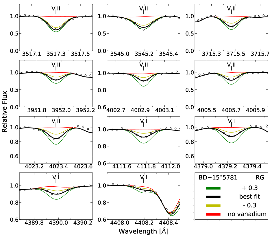
Figure 1: Observed (points) and synthetic (lines) spectra for a representative red giant, BD $-$15^∘5781. The first seven lines shown are V ii lines, while the last four lines are V i lines. The best-fit lines are for each line individually. Note that the vertical axis range is adjusted for some of the weak lines to provide a clearer visualization of the best fit.

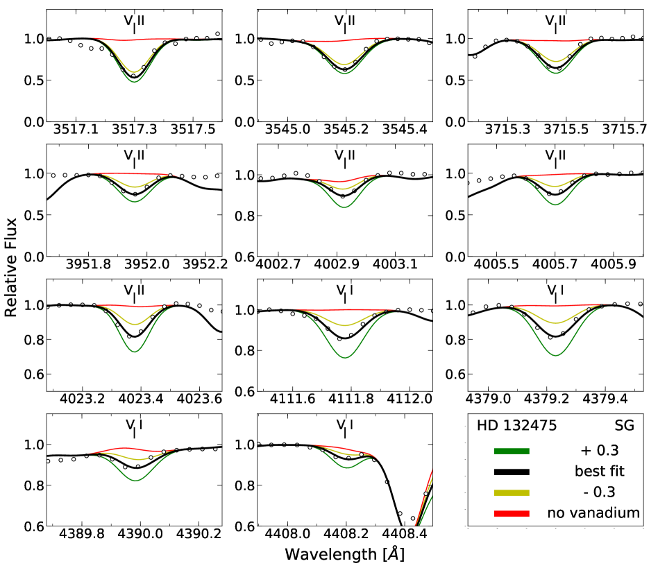
Figure 2: Observed (points) and synthetic (lines) spectra for a representative sub-giant, HD 132475.

Table 2: Abundances Derived from Neutral Vanadium Lines

Star	Wavelength (Å)	$\log\epsilon$ (V i)	$\sigma$
BD $+$10∘2495	4111.779	1.51	0.10
BD $+$10∘2495	4379.230	1.39	0.06
BD $+$10∘2495	4389.979	1.42	0.10
BD $+$10∘2495	4408.196	1.33	0.20
BD $+$19∘1185a	4111.779	2.44	0.20
BD $+$19∘1185a	4379.230	2.53	0.10
BD $+$19∘1185a	4389.979	2.56	0.15
BD $+$19∘1185a	4408.196	2.38	0.10

Note. — The model atmosphere uncertainty is not included in here for reasons discussed in Section 3.3. The complete version of Table 2 is available in the online edition of the journal. A short version is included here to demonstrate its form and content.

Table 3: Abundances Derived from Ionized Vanadium Lines

Star	Wavelength (Å)	$\log\epsilon$ (V ii)	$\sigma$
BD $+$10∘2495	3715.464	1.70	0.17
BD $+$10∘2495	3951.957	1.77	0.18
BD $+$10∘2495	4002.928	1.69	0.11
BD $+$10∘2495	4005.702	1.87	0.15
BD $+$10∘2495	4023.377	1.87	0.11
BD $+$19∘1185a	3715.464	2.74	0.18
BD $+$19∘1185a	3951.957	2.76	0.14
BD $+$19∘1185a	4002.928	2.71	0.20
BD $+$19∘1185a	4005.702	2.86	0.06

Note. — The model atmosphere uncertainty is not included in here for reasons discussed in Section 3.3. The complete version of Table 3 is available in the online edition of the journal. A short version is included here to demonstrate its form and content.

3.3 Uncertainties

The statistical uncertainty for $\log\epsilon$(V) of each line includes the fitting uncertainty of the measurement and the uncertainty in the $\log gf$ of the line transition (Lawler et al., 2014; Wood et al., 2014). The fitting uncertainties are estimated based on the spectrum synthesis matching. The typical fitting uncertainty for the sample is approximately 0.15 dex. In most cases, the fitting uncertainty is much larger than the transition probability uncertainty, because the lines we adopted are all major branches that are understood and measured to great precision (typically 0.02 dex uncertainty) in the laboratory. For each given star, we weight the vanadium abundance measurement from each line by the inverse-square of the statistical uncertainty to calculate the total statistical uncertainty of the star. In cases when the few measurements agree exactly, we set an arbitrary minimum statistical weighted uncertainty of 0.05 dex.

The abundance uncertainty introduced by the uncertainties in the model atmosphere parameters is extracted from the vanadium abundances derived by Roederer et al. (2014). Although we use more lines in this work, we still decided to adopt the same model atmosphere uncertainties. While individual lines with different E.P. will have different model $T_{\rm eff}$ sensitivities, the lines we have used here have a very similar range of E.P. as the ones used in Roederer et al. (2014), as shown in Table 1. Thus we expect the newly added lines will respond to the model atmosphere parameter uncertainties similarly to the lines used in the previous work. We combine the extracted model atmosphere uncertainties with the total fitting statistical uncertainties.

Our study has made several improvements relative to Roederer et al. (2014) that reduce the overall abundance uncertainties in most stars. In particular, we use improved atomic transition data with almost negligible uncertainties in the $\log gf$ value of the line. More importantly, we use more lines so that we have better statistics. The statistical uncertainty approaches the fitting uncertainty as the number of lines we use for each star increases, assuming there is no intrinsic scattering in the vanadium measurement from different lines. The typical size of this statistical uncertainty is 0.10 for the 50 most metal-poor stars and 0.08 for the 50 most metal-rich stars. Yet, the final total uncertainties are dominated by the model uncertainty because the typical size of the model atmosphere uncertainties is approximately 0.17. On average, the total uncertainties increase by only a small amount ($<10$%) as we move from the metal-rich to the metal-poor stars.

3.4 Internal Comparisons

Stars with just one measured V i or V ii transition have larger star-to-star scatter in a given [Fe/H] domain than do stars with multiple measurements. We perform statistical tests to determine if single-line abundance results should be dropped from further analyses. Statistical tests (KS test, Kolmogorov 1933; Smirnov 1948; Anderson test, Stephens 1974; Mann-Whitney U test, Mann & Whitney 1947) show a strong indicator that the stars with only one measurement are not drawn from the same distribution as the stars with multiple measurements. The KS test, for example, gives a p-value of $1.15\times 10^{-9}$. We thus treat these stars with less confidence and advise readers to be cautious when using these measurements for other purposes. In most of the figures, we use “x” s to indicate the stars with only one measurement, and we exclude these stars from further analysis of the aggregated sample.

To examine the consistency between spectra taken by different telescopes and instruments, we examined the five stars that are observed multiple times with MIKE, MCD, and HET: HD 106373, HD 108317, HD 122563, HD 132475, and HE 1320-1339. All of these stars have one observation in MIKE, and another observation in MCD.  HD 122563 was also observed with the HET.  We find good agreement, both through a line-by-line abundance comparison and a weighted average abundance comparison. As shown in Figure 3, most of the results agree to within 1$\sigma$, which we consider to be satisfactory.

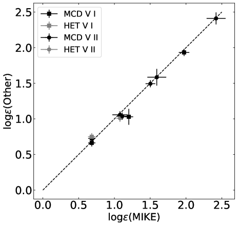
Figure 3: Comparison of the stars observed with multiple spectrographs in the sample. Each data point represents a star, and the position of the data point represents their derived $\log\epsilon$ value from different spectra. The black dots give the comparison between MIKE and MCD, and the gray square gives the comparison between MIKE and HET.  The dashed line represents perfect agreement.

3.5 Comparison with Previous Results

We compare our derived $\log\epsilon$(V) values to those obtained previously by Roederer et al. (2014). We find in general good agreement between them as shown in the top panels of Figure 4. The offsets remain consistent with zero within 1$\sigma$ as shown in Figure 5. Furthermore, the remaining offsets (0.05 dex for V i and 0.06 dex for V ii) can be entirely explained by the differences in the $\log gf$ values adopted by each study. We also examine the uncertainties in these values. The bottom panels of Figure 4 compare the uncertainties derived by Roederer et al. (2014) with those derived in our work. As expected, the uncertainties are in general improved, especially for abundances derived from V ii lines, thanks to the improved atomic transition data and increased number of lines used. Comparing the stars that have measurements in both studies, we improve the median uncertainties in the logarithmic abundances by 27 % (from 0.13 to 0.09 dex) for V i and 26 % (from 0.27 to 0.20 dex) for V ii.

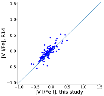
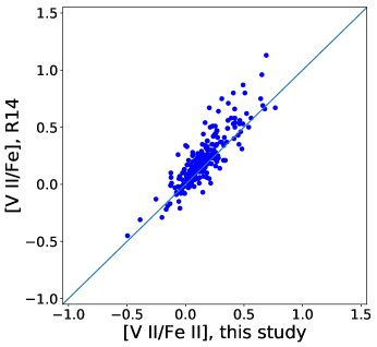
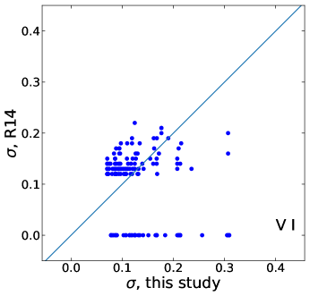
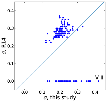
Figure 4: Comparison of the [V/Fe] ratios and the uncertainties with those from Roederer et al. (2014) (R14). The blue lines represents perfect agreement between the two studies. The points at y=0.0 in the $\sigma$ plots correspond to stars with no measurement of V in the R14 sample.

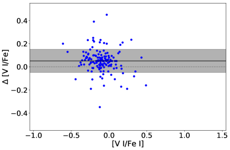
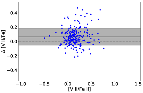
Figure 5: The difference between this study and Roederer et al. (2014) as a function of the [V/Fe] ratios derived in this work. The dashed line represents no difference. The solid black line and the gray band represent the mean and 1$\sigma$ interval of the differences.

We also compared our result with the metal-poor star HD 84937 studied extensively in Lawler et al. (2014), Wood et al. (2014), and Sneden et al. (2016). Using spectra that cover a wider wavelength range, those studies provided detailed chemical abundances for this star with updated transition data, which we have also used in this work. As a consistency check, we adopt the ATLAS9 AODFNEW model with stellar parameters adopted by these previous studies ($T_{\rm eff}$ = 6300 K, log g = 4.0, [Fe/H] = $-2.15$, $v_{\rm t}$ = 1.5 km s^-1). We obtain individual line measurements that agree with those from Lawler et al. (2014) for V i and Wood et al. (2014) for V ii with differences $\leq$ 0.03 dex, which is well within our measurement uncertainty. For mean abundances, Sneden et al. (2016) reported $\log\epsilon(\text{V}~{}\textsc{i})=1.890\pm 0.070$ from 9 lines and $\log\epsilon(\text{V}~{}\textsc{ii})=1.871\pm 0.075$ from 68 lines. After applying the same calibration applied to all other stars in our sample (see Section 3.6), we obtain $\log\epsilon(\text{V}~{}\textsc{ii})$ = 1.95, giving [V ii/Fe ii] $=+0.33$. For V i, we detect only the line at 4379 Å.  The single measurement, $\log\epsilon(\text{V}~{}\textsc{i})=1.87$, gives [V i/Fe i] = +0.26. Both agree with the Sneden et al. (2016) values.

3.6 Trends with Wavelength

As discussed extensively in Roederer et al. (2012, 2014, 2018), the continuous opacity is mainly contributed by the H^- in the atmosphere for most of the stars in our sample, with a minor contribution from the bound-free opacity from H i. At wavelengths shorter than the Balmer limit at $\approx 3647$ Å, the bound-free opacity increases from the Paschen continuum to the Balmer continuum with a discontinuous jump, causing an overall increase in the overall continuous opacity. This change in the continuous opacity may not be fully and accurately accounted for in the spectrum synthesis, possibly leading to underestimated results for the vanadium abundances from the four shortest wavelength lines (3517.299 Å, 3545.196 Å, 3715.464 Å, and 3951.957 Å), as shown in Figure 6. Neglecting 3D convection effects could also lead to a similar result, which explains why some species experience this effect but others may not (see discussion in Roederer et al. 2018). Underestimated log g values will not explain the low abundances from lines at wavelengths shorter than the Balmer limit because changing changing the log g values of the model atmosphere would similarly affect the abundances derived from all V ii lines examined in this study.

This so-called “Balmer Dip Effect” is significant for about half of the available V ii lines. We decided it is necessary to apply an empirical calibration to the four shortest wavelength V ii lines. The calibration is determined based on the weighted average $\log\epsilon$(V ii) for each star computed with only the three longest wavelength lines (4002.928 Å, 4005.702 Å, and 4023.377 Å), which we have taken to be the correct vanadium abundance and are not affected by the continuum change.

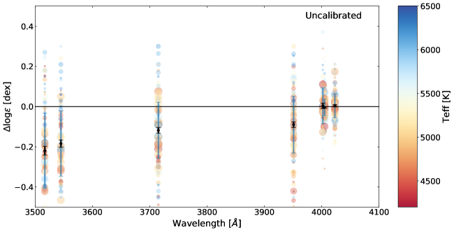
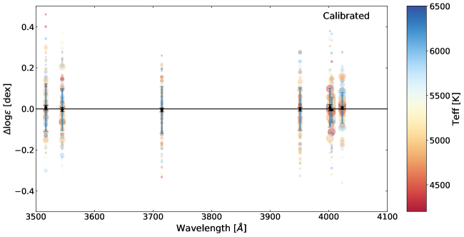
Figure 6: The difference between the fitting from an individual line and the average calculated from the three longest wavelength lines, averaged over all stars with MIKE data, before calibration (top panel) and after calibration (bottom panel). The horizontal line represents no offset relative to the mean abundance derived from the three lines with $\lambda>4000$ Å.  The data points are color coded by temperature, with point size determined by the uncertainty in the measurement.

To keep consistency in how each star in the sample contributes to determining the calibration, we assessed the calibration using only the stars observed with MIKE, as only they have spectra extended across all seven lines. This effect is most significant in cooler stars, and it gets weaker as the temperature increases. We separate the MIKE stars into four temperature groups and fit a line to determine the amount of calibration needed for each line as a function of temperature. The fitting and its corresponding uncertainty is conducted using the Scipy package $curve\_fit$ function (Jones et al., 2001), which is essentially least-squares fitting. The result is shown in Figure 7.

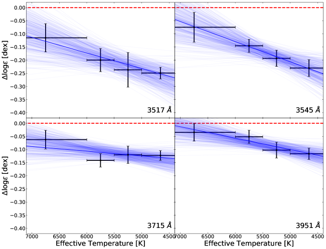
Figure 7: The calibration fitting for the four bluest V ii lines that are affected by the Balmer region continuum effect. The horizontal error bars represent the range of $T_{\rm eff}$ of the stars that are used to generate the data point. The vertical error bars represent the uncertainty in the offset that needs to be calibrated for the particular $T_{\rm eff}$ group. The set of lines in the figure is generated using a Monte Carlo method to provide a visualization of the fitting uncertainty. They are generated by fitting the resampled offsets from the four $T_{\rm eff}$ groups.

After applying the calibration, the measurements from the calibrated four lines (3517.299 Å, 3545.196 Å, 3715.464 Å, and 3951.957 Å) are able to statistically match the measurements from the other three lines within 1$\sigma$. However, due to the uncertainties introduced by the calibration, these calibrated data now receive a lower weight in determining the final abundance for each star, as shown in Figure 6. We also point out that the same calibration is applied to the upper limits.

The V i lines we used are in a longer wavelength region that is not affected, so no calibrations are applied to them.

3.7 Final Abundances

In total, we have 190 stars in this sample with V i detections (including 10 without V ii) from 4 lines, 251 stars with V ii detections (including 71 without V i) from 7 lines, and 255 stars with either V i or V ii. After the calibration has been applied, we weight the vanadium measurements by their overall uncertainties to calculate the final abundance for each star. We combine the measurements from the seven ionized lines, and the four neutral lines, to generate the ionized and neutral abundances of vanadium respectively. The final abundances are shown in Table 4. Figure 8 shows the [V/Fe] ratios as a function of metallicity. In the metallicity range $-$4.0 $<$ [Fe/H] $<-$1.0, the mean [V i/Fe i] ratio is [V i/Fe i] $=-0.10\pm 0.01~{}(\sigma=0.16)$ dex from 128 stars with $\geq$ 2 V i lines detected, and the mean [V ii/Fe ii] ratio is [V ii/Fe ii] $=+0.13\pm 0.01~{}(\sigma=0.16)$ dex from 220 stars with $\geq$ 2 V ii lines detected.

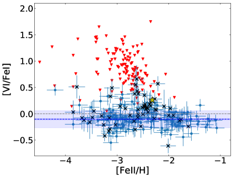
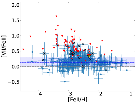
Figure 8: [V/Fe] as a function of metallicity. The blue dots are detections, red triangles are upper limits, and black crosses are stars with only one line detected. The yellow star is HD 84937. The blue lines represent the weighted average of the whole sample calculated using stars with $\geq$ 2 lines of a given V species detected. The bands represent 1$\sigma$ intervals.

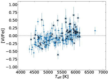
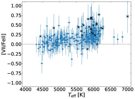
Figure 9: [V/Fe] as a function of $T_{\rm eff}$. Note that the upper limits and the stars with only one detected line are excluded.

Table 4: Final Abundances for the Sample

						V i						V ii
Star	Class	$T_{\rm eff}$(K)	log g	[Fe i/H]	[Fe ii/H]	U. L.	U. L. $\lambda$	[V i/Fe i]	$\sigma$	$N$		U. L.	U. L. $\lambda$	[V ii/Fe ii]	$\sigma$	$N$
BD $+$10∘2495	RG	4890	1.85	-2.16	-2.14	0	–	-0.36	0.10	4		0	–	-0.01	0.19	5
BD $+$19∘1185a	MS	5440	4.30	-1.25	-1.25	0	–	-0.21	0.12	4		0	–	0.15	0.14	4
BD $+$24∘1676	SG	6140	3.75	-2.70	-2.54	1	4111.779	0.81	–	0		0	–	0.32	0.23	3
BD $+$26∘3578	SG	6060	3.75	-2.60	-2.41	0	–	0.10	0.14	1		0	–	0.22	0.22	2
BD $+$29∘2356	RG	4710	1.75	-1.73	-1.62	0	–	-0.24	0.20	1		0	–	0.16	0.18	4
BD $+$44∘0493	RG	5040	2.10	-4.28	-4.26	1	4111.779	1.27	–	0		1	3715.464	0.97	–	0

Note. — The complete version of Table 4 is available in the online edition of the journal. A short version is included here to demonstrate its form and content.

4 Results

4.1 Trends with Stellar Parameters

We first examine the [V/Fe] abundance ratios as a function of $T_{\rm eff}$ in Figure 9. There is a difference of about 0.3 dex in the mean [V/Fe] ratios between the coolest stars (around 4500 K) and the warmest stars (around 6200 K), with the warmest stars showing higher [V/Fe] ratios on average. Trends that are similar in both magnitude and direction are found among the [Sc/Fe], [Ti/Fe], [Cr/Fe], and [Mn/Fe] ratios in the Roederer et al. (2014) sample, leading us to conclude that the stellar parameters and Fe abundances are responsible for these trends. Resolving the issue could require a reanalysis of the stellar parameters and metallicities for the entire sample, which is beyond the scope of the present study.

We also examine the [V/Fe] abundance ratios as a function of [Fe/H] and stellar evolutionary state in Figure 10. We regard the [V ii/Fe] ratios to be better representations of the [V/Fe] ratios in these stars than the [V i/Fe] ratios, which are likely subject to departures from LTE (Section 4.2). Among the red giants in the sample, which extend across the widest range in metallicity (roughly $-4.0<$ [Fe/H] $<-1.5$), there is no dependence of [V ii/Fe] on [Fe/H].

The trend of increasing [V/Fe] ratios with decreasing metallicity among subgiants is likely caused by the fact that we need a much stronger line to get a valid detection from these warm, low-metallicity stars. The higher the temperature, as well as the lower the metallicity and vanadium abundance, the higher that limit is. We perform a separate test to determine where those limits lie. We generate model atmospheres at several typical temperatures and metallicities that resemble the actual sample. Using these hypothetical model atmospheres, we determine the minimum detectable abundance based on our synthetic spectra.  The stars with one or no vanadium lines detected are consistent with these tests.

Many of the subgiants at the lower metalliciy end in Figure 10 have only one detection from the strongest line. Since these stars have only one detection, and that detection lies near the limit for minimum detectable vanadium abundances, we decide to exclude them from subsequent analyses. When we examine correlations between vanadium and other iron-group elements (Section 4.3), these stars are not included or shown in the figures.

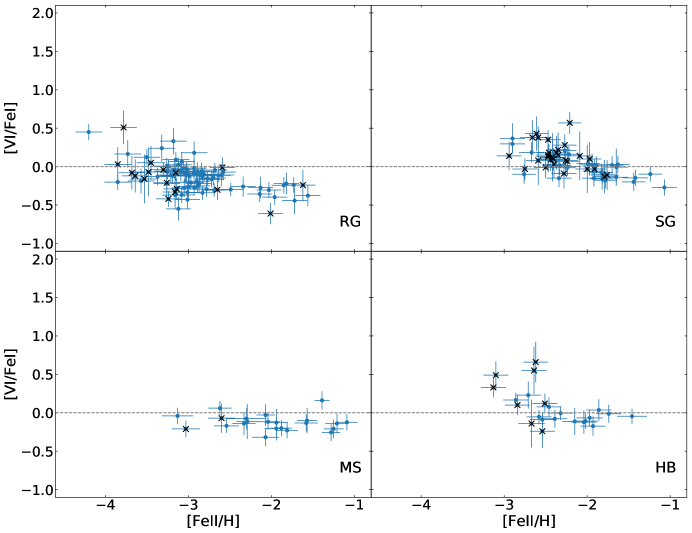
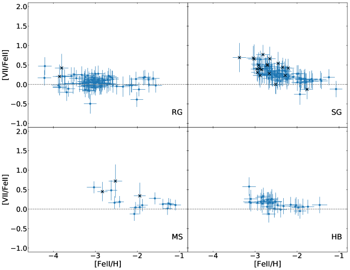
Figure 10: [V/Fe] as a function of metallicity in separate class groups. The legend is the same as in Figure 8, and upper limits have been omitted.

We also investigate the impact of the stellar parameter uncertainties on the derived [V/Fe] ratios. For this test, we select two representative red giants with similar stellar parameters and metallicities (HD 21581 (catalog HD 21581): $T_{\rm eff}$ = 4940 K, log g = 2.10, $v_{\rm t}$ = 1.50 km s^-1, [Fe/H] = $-$1.82; HD 126238 (catalog HD 126238): $T_{\rm eff}$ = 4750 K, log g = 1.65, $v_{\rm t}$ = 1.55 km s^-1, [Fe/H] = $-$1.96) and contrasting vanadium abundances ([V ii/Fe ii] = $+$0.19, derived from 6 V ii lines; and [V ii/Fe ii] = $-$0.13, derived from 7 V ii lines, respectively). We resample the stellar parameters $10^{3}$ times assuming normal error distributions on $T_{\rm eff}$, log g, $v_{\rm t}$, and [M/H], and we recompute the vanadium abundances for each new combination of parameters. The resamples include the dependence of log g on $T_{\rm eff}$ through the $\text{Y}^{2}$ isochrones. For this test, we approximate the abundances derived via spectrum synthesis as equivalent widths.

Figure 11 illustrates the results of this test. Three important features are found. First, the [V/Fe] ratios from lines of both neutral and ionized species show minimal sensitivity to variations in the stellar parameters. Secondly, the [V/Fe] ratio is consistently higher when derived from lines of ionized atoms than lines of neutral atoms (see also Section 4.2). Finally, the contrast between the high [V/Fe] ratio in HD 21581 (catalog HD 21581) and the low [V/Fe] ratio in HD 126238 (catalog HD 126238) is always present, suggesting that there are intrinsic [V/Fe] differences from one star to another (see also Section 4.3). These three behaviors are largely unaffected by uncertainties in the stellar parameters.

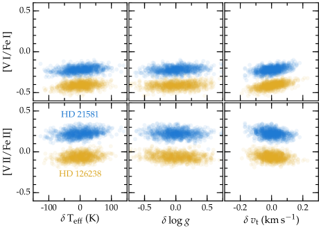
Figure 11: Comparison of the [V/Fe] ratios for two representative red giants as a function of changes in the stellar parameters. The blue points represent the results for HD 21581 (catalog HD 21581), and the yellow points represent the results for HD 126238 (catalog HD 126238). The three columns represent changes in $T_{\rm eff}$, log g, and $v_{\rm t}$ relative to the median value of each parameter. Notice that there is minimal change in the [V/Fe] ratio for each star, whether derived from lines of the neutral or ionized species, and the high value of [V/Fe] in HD 21581 (catalog HD 21581) robustly remains in contrast to the low value of [V/Fe] in HD 126238 (catalog HD 126238).

4.2 Possible Non-LTE Effects

We examine possible non-LTE effects by comparing the vanadium abundance derived from neutral vanadium and that from ionized vanadium. Our calculations are made assuming LTE Saha ionization equilibrium. We see in Figure 12 that the neutral vanadium lines give slightly lower vanadium abundances than the ionized vanadium lines, [V ii/V i] $=+0.25\pm 0.01~{}(\sigma=0.15)$ dex from 119 stars. This suggests that non-LTE effects may be important, and we assume that over-ionization of neutral vanadium is occurring. No non-LTE studies of vanadium abundances in late-type stars have been conducted, and we encourage non-LTE calculations for neutral vanadium in the future to test this hypothesis and obtain more accurate results for abundances derived from V i lines.

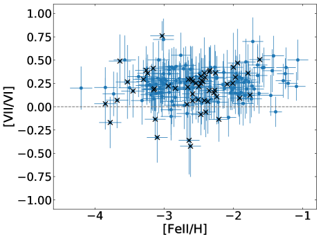
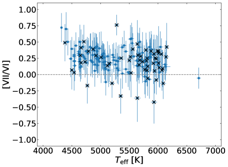
Figure 12: Comparison of [V ii/V i] as a function of [Fe/H] (top) and $T_{\rm eff}$ (bottom).

The V ii lines we use are connected to the low metastable levels of the ion, which are the primary population reservoir levels for vanadium in the atmospheres of late-type stars. Therefore, we consider the abundances derived from the V ii lines to be less affected by non-LTE effects, and they should provide more accurate abundances (cf. Lawler et al. 2013).

When calculating the vanadium abundance ratio using the neutral lines, we use the iron abundance derived from the neutral iron species for consistency, and vice versa for the abundance ratio derived from the ionized vanadium lines. We note this fact by writing [V i/Fe i] and [V ii/Fe ii] when possible. Furthermore, when we examine the correlations between the vanadium abundances derived in this study and other iron-group elements from Roederer et al. (2014) (Section 4.3), we compare abundances derived from neutral iron-group species with those from neutral vanadium and abundances derived from ionized iron-group species with those from ionized vanadium.

4.3 Correlation with Other Iron-group Elements

We observed in Section 4.1 that there are intrinsic differences in the [V/Fe] ratios found among this sample of stars, and we showed that these differences are not a consequence of uncertainties in the stellar parameters. These differences also cannot be attributed to the $\log gf$ values. Systematic uncertainties in the laboratory $\log gf$ values for all of the lines of iron-group elements considered here—including scandium, titanium, and vanadium—are small (typically $<$ 5 % or $<$ 0.02 dex), so they are effectively negligible in the abundance error budget.

Following Sneden et al. (2016) and Cowan et al. (2020), we examine whether these differences may be related to correlations among scandium, titanium, and vanadium. For this test, we adopt the abundances of other iron-group elements presented by Roederer et al. (2014). For completeness, we examine whether correlations exist between all other pairs of iron-group elements. We check for correlations in the [X/Fe] ratios, where X represents Sc ii, Ti i, Ti ii, V i, V ii, Cr i, Cr ii, Mn i, Mn ii, Co i, and Ni i.

Since the abundances are all derived quantities, we apply an orthogonal distance regression (ODR) to the sample to obtain the slope as a measure of the correlation. To incorporate the uncertainties in the measurements, we generate 1000 re-samplings of the measurements based on the uncertainties, and we apply ODR to the re-sampled data. Because the slope distributions for most pairs of elements are not Gaussian, the medians are taken as the final results, with the 16 % and 84 % intervals as the standard deviations. We compute the significance of the correlation as the slope divided by the standard deviation. Other fitting methods, such as the merit function maximization and the Markov chain Monte Carlo (MCMC) method, yield consistent results. The fitting results over the entire sample are shown in Figure 13. The figure shows the significance of the correlation between each possible pair of iron-group elements by the shade. For example, the slope of [V i/Fe] versus [Ti i/Fe] is $2.07\pm 0.29$ with a significance greater than 7$\sigma$, whereas [Cr ii/Fe] versus [V ii/Fe] has slope $0.06\pm 0.06$ with a significance less than 1$\sigma$. Among all the correlations involving vanadium, we see more significant correlations with ionized scandium and neutral as well as ionized titanium. The ODR gives significance for these correlation greater than 3$\sigma$. We present the three correlation fits between scandium, titanium, and vanadium in Figure 14 to better illustrate the significance of the correlation slope. We also apply the ODR to subgroups divided according to metallicities and evolutionary stages and obtain results that agree with the behavior of the full sample.

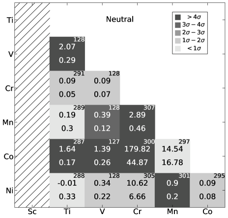
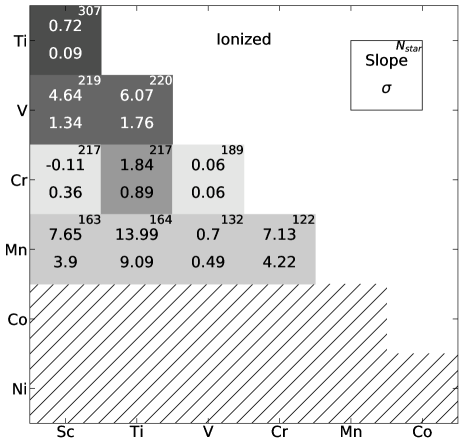
Figure 13: A summary of the slopes for the correlation fittings between 11 iron-group species, expressed as [X/Fe], with neutral species in the upper panel and ionized species in the lower panel. The color of the squares represent the significance of the correlation, as indicated in the upper panel. The meaning of the numbers are given in the lower panel, where slope is the median of the slopes from 1000 resampling, $\sigma$ is distance from the median to the 16 % and 84 % intervals, and $N_{star}$ is the number of stars used in each correlation calculation. The hatching indicates correlations where we have no available abundances to perform the fitting.

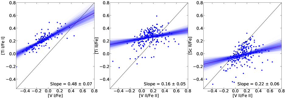
Figure 14: Correlation fitting for three pairs of iron-group elements. The panels show the high-significance correlations between scandium, titanium, and vanadium. The best fit recorded in Figure 13 is plotted as the solid line, with all 1000 re-samplings plotted in low opacity. A 45^∘ dashed line is included for comparison. Note the axes are swapped as compared to the correlation fits shown in Figure 13 to keep vanadium consistently on the x-axis. The slope printed at the lower right corner of each panel is changed accordingly, but they maintain the same significance as a result of ODR.

These correlations among scandium, titanium, and vanadium cannot be a consequence of the correlations with $T_{\rm eff}$ that were noted in Section 4.1. If they were, then we would also expect to see correlations between these elements and chromium and manganese; no significant correlations are detected between chromium or manganese and scandium or titanium, and there are other reasons to disfavor those between vanadium, chromium, and manganese (see below). Furthermore, as shown by Cowan et al. (2020), correlations among scandium, titanium, and vanadium are detected in multiple independent datasets whose stars do not show any correlations with $T_{\rm eff}$.

We also notice significant correlations between cobalt, manganese, and other elements. In particular, [Co i/Fe i] shows significant correlations with [Ti i/Fe i], [V i/Fe i], and [Cr i/Fe i]. We present the correlation fits of vanadium with chromium, manganese, cobalt, and nickel in Figure 15. There are, however, reasons to discount these other correlations. As pointed out by Cowan et al. (2020), neutral cobalt, which is a trace species, yields substantially higher abundances than ionized cobalt in the three metal-poor stars examined in that study. Non-LTE effects on the abundance derived from Co i lines can be substantial (Bergemann et al., 2010). Cowan et al. concluded that the abundances derived from neutral cobalt likely are not correct. Although we do not have cobalt measurements from Co ii lines to make the same comparison for our sample, it is likely that our neutral cobalt measurements are affected by the same issue. Any correlations between cobalt and other iron-group elements found here should be treated with caution.

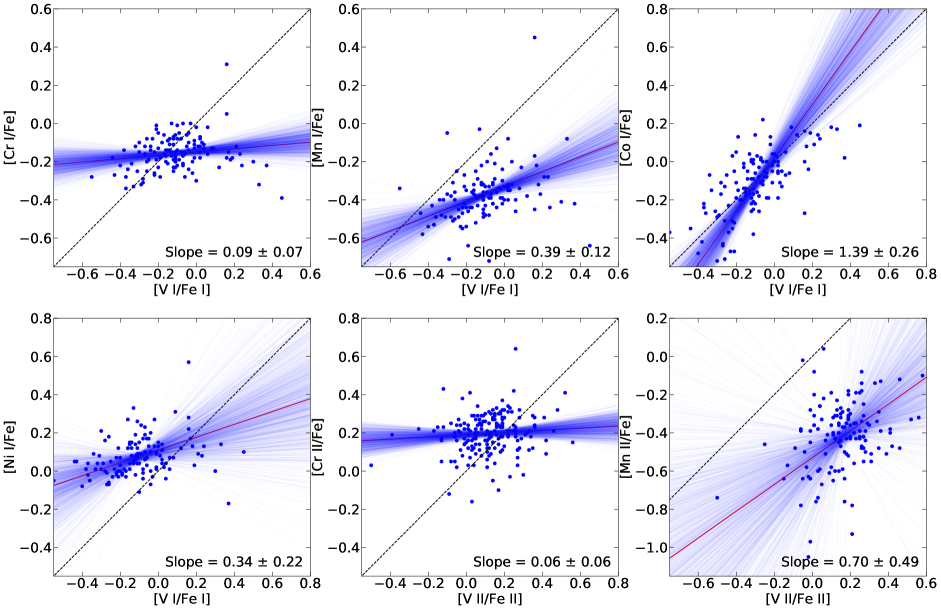
Figure 15: Correlation fitting for six pairs of iron-group elements. The panels show the correlations between vanadium, chromium, manganese, cobalt, and nickel. The first, fourth, fifth, and sixth correlations are not significant, whereas the second and third are significant. For reasons stated in the text, we conclude the correlations among vanadium, manganese, and cobalt are not reliable.

Non-LTE effects may also be responsible for correlations involving neutral titanium, vanadium, chromium, manganese, and nickel. These elements have low first ionization potentials ($<$ 7.7 eV), so their neutral species are distinct minorities in the atmospheres of the stars in our sample. Previous calculations have shown that non-LTE effects can be significant (e.g., Ti: Sitnova et al. 2020; Cr: Bergemann & Cescutti 2010; Mn: Bergemann & Gehren 2008). No non-LTE studies of nickel abundances are available, but nickel has a similarly low first ionization potential, so levels of its neutral species could reasonably be expected to deviate from their LTE populations.

These concerns motivate our recommendation to favor the correlation results derived from the majority ion species and disfavor the results derived from the neutral species. As shown in the bottom panel of Figure 13, scandium, titanium, and vanadium correlate significantly with each other, and similar correlations are not found among chromium or manganese. We conclude these observed correlations most likely arise from the production mechanism rather than systematic or observational effects.

5 Discussion

The super-solar [V ii/Fe] ratio indicates a potential dominance of massive Type II SNe in early Galactic nucleosynthesis, because vanadium is more abundantly produced by more massive Type II SNe (Chieffi & Limongi, 2004). Environments with more massive Type II SNe would also explain the super-solar ratios of titanium. The correlated scandium, titanium, and vanadium abundances suggest that these three elements may be produced under similar conditions. Titanium is sometimes referred to as an $\alpha$ element. It seems unlikely, however, that these three elements are produced along with the $\alpha$ elements in the SNe that enriched the stars in our sample. As discussed in Curtis et al. (2019), Cowan et al. (2020), and references therein, the nucleosynthesis origin of these elements in Type II SNe occurs mainly in proton-rich inner layers during complete silicon burning. Their production is complex, and current models remain unable to fully reproduce the observed abundance ratios.

The correlations we identify are not related to those found among more metal-rich stars. In near-solar metallicity stars, for example, Hasselquist et al. (2017) pointed out that vanadium and manganese are expected to be more metallicity-dependent than iron, causing the relative abundances of these two elements to increase with metallicity (Andrews et al., 2017). It is indeed observed that [V/Fe] and [Mn/Fe] increase with [Fe/H] in the Milky Way (MW) and Sagittarius (Sgr) dwarf galaxy samples, although both ratios are deficient in Sgr relative to the MW.  This metallicity-dependent correlation is different from the one identified in the present study, which focuses on much more metal-poor stars where minimal metallicity dependence is observed in the [V/Fe] ratios.

6 Conclusions

Using improved atomic transition data, we rederived the vanadium abundances for 255 metal-poor stars from Roederer et al. (2014). With an increase from 3 to 11 lines used, we obtained consistent measurements with the previous study but smaller uncertainties. As shown in Section 4, our work further supports the existence of correlations between scandium, titanium, and vanadium in metal-poor stars. With many more lines used, we have greater confidence in the reliability of these rederived vanadium abundances. By examining trends of individual lines and overall abundances with stellar parameters, we have identified no systematic effects in the analysis that could account for the correlations observed. We conclude that the correlations are, therefore, very likely a result of nucleosynthesis at early Galactic time.

As summarized in Section 1, we do not yet have an explanation for the correlations, especially between scandium, titanium, and vanadium. The complex production history of scandium in CCSNe makes it difficult to understand how it is related to vanadium and titanium (Sneden et al., 2016). It is possible to reproduce the overall iron-group element abundances by including a larger hypernova fraction and taking into account the effect of neutrino interactions and jets (Umeda & Nomoto, 2002; Kobayashi et al., 2006, 2011; Curtis et al., 2019). Yet, it is still unclear how the current CCSNe models will impact the GCE calculations, and whether they can reproduce the correlations seen in observations. More theoretical works are needed to explain the correlations between scandium, titanium, and vanadium.

References

- Andrews et al. (2017) Andrews, B. H., Weinberg, D. H., Schönrich, R., & Johnson, J. A. 2017, The Astrophysical Journal, 835, 224, doi: 10.3847/1538-4357/835/2/224
- Asplund et al. (2009) Asplund, M., Grevesse, N., Sauval, A. J., & Scott, P. 2009, ARA&A, 47, 481, doi: 10.1146/annurev.astro.46.060407.145222
- Barklem et al. (2005) Barklem, P. S., Christlieb, N., Beers, T. C., et al. 2005, A&A, 439, 129, doi: 10.1051/0004-6361:20052967
- Bergemann & Cescutti (2010) Bergemann, M., & Cescutti, G. 2010, A&A, 522, A9, doi: 10.1051/0004-6361/201014250
- Bergemann & Gehren (2008) Bergemann, M., & Gehren, T. 2008, A&A, 492, 823, doi: 10.1051/0004-6361:200810098
- Bergemann et al. (2010) Bergemann, M., Pickering, J. C., & Gehren, T. 2010, MNRAS, 401, 1334, doi: 10.1111/j.1365-2966.2009.15736.x
- Bernstein et al. (2003) Bernstein, R., Shectman, S. A., Gunnels, S. M., Mochnacki, S., & Athey, A. E. 2003, in Proc. SPIE, Vol. 4841, Instrument Design and Performance for Optical/Infrared Ground-based Telescopes, ed. M. Iye & A. F. M. Moorwood, 1694–1704, doi: 10.1117/12.461502
- Bressan et al. (2012) Bressan, A., Marigo, P., Girardi, L., et al. 2012, MNRAS, 427, 127, doi: 10.1111/j.1365-2966.2012.21948.x
- Cayrel et al. (2004) Cayrel, R., Depagne, E., Spite, M., et al. 2004, A&A, 416, 1117, doi: 10.1051/0004-6361:20034074
- Chieffi & Limongi (2004) Chieffi, A., & Limongi, M. 2004, The Astrophysical Journal, 608, 405, doi: 10.1086/392523
- Cohen et al. (2008) Cohen, J. G., Christlieb, N., McWilliam, A., et al. 2008, ApJ, 672, 320, doi: 10.1086/523638
- Cohen et al. (2004) —. 2004, ApJ, 612, 1107, doi: 10.1086/422576
- Cowan et al. (2020) Cowan, J. J., Sneden, C., Roederer, I. U., et al. 2020, ApJ, 890, 119, doi: 10.3847/1538-4357/ab6aa9
- Curtis et al. (2019) Curtis, S., Ebinger, K., Fröhlich, C., et al. 2019, ApJ, 870, 2, doi: 10.3847/1538-4357/aae7d2
- Demarque et al. (2004) Demarque, P., Woo, J.-H., Kim, Y.-C., & Yi, S. K. 2004, ApJS, 155, 667, doi: 10.1086/424966
- Gratton et al. (2000) Gratton, R. G., Sneden, C., Carretta, E., & Bragaglia, A. 2000, A&A, 354, 169
- Gustafsson et al. (2008) Gustafsson, B., Edvardsson, B., Eriksson, K., et al. 2008, A&A, 486, 951, doi: 10.1051/0004-6361:200809724
- Hasselquist et al. (2017) Hasselquist, S., Shetrone, M., Smith, V., et al. 2017, The Astrophysical Journal, 845, 162, doi: 10.3847/1538-4357/aa7ddc
- Hunter (2007) Hunter, J. D. 2007, Computing in Science and Engineering, 9, 90, doi: 10.1109/MCSE.2007.55
- Jones et al. (2001) Jones, E., Oliphant, T., Peterson, P., & et al. 2001, SciPy: Open source scientific tools for Python, online. http://www.scipy.org/
- Kobayashi et al. (2011) Kobayashi, C., Karakas, A. I., & Umeda, H. 2011, Monthly Notices of the Royal Astronomical Society, 414, 3231, doi: 10.1111/j.1365-2966.2011.18621.x
- Kobayashi et al. (2006) Kobayashi, C., Umeda, H., Nomoto, K., Tominaga, N., & Ohkubo, T. 2006, The Astrophysical Journal, 653, 1145, doi: 10.1086/508914
- Kolmogorov (1933) Kolmogorov, A. N. 1933, G. Ist. Ital. Attuari., 4, 83
- Kramida et al. (2018) Kramida, A., Ralchenko, Y., Reader, J., & NIST ASD Team. 2018, NIST Atomic Spectra Database (ver. 5.5.6), [Online]. Available: https://physics.nist.gov/asd, National Institute of Standards and Technology, Gaithersburg, MD.
- Lai et al. (2008) Lai, D. K., Bolte, M., Johnson, J. A., et al. 2008, ApJ, 681, 1524, doi: 10.1086/588811
- Lawler et al. (2013) Lawler, J. E., Guzman, A., Wood, M. P., Sneden, C., & Cowan, J. J. 2013, ApJS, 205, 11, doi: 10.1088/0067-0049/205/2/11
- Lawler et al. (2014) Lawler, J. E., Wood, M. P., Den Hartog, E. A., et al. 2014, ApJS, 215, 20, doi: 10.1088/0067-0049/215/2/20
- Mann & Whitney (1947) Mann, H. B., & Whitney, D. R. 1947, Ann. Math. Statist., 18, 50, doi: 10.1214/aoms/1177730491
- Roederer et al. (2014) Roederer, I. U., Preston, G. W., Thompson, I. B., et al. 2014, AJ, 147, 136, doi: 10.1088/0004-6256/147/6/136
- Roederer et al. (2018) Roederer, I. U., Sneden, C., Lawler, J. E., et al. 2018, ApJ, 860, 125, doi: 10.3847/1538-4357/aac6df
- Roederer et al. (2012) Roederer, I. U., Lawler, J. E., Sobeck, J. S., et al. 2012, ApJS, 203, 27, doi: 10.1088/0067-0049/203/2/27
- Sitnova et al. (2020) Sitnova, T. M., Yakovleva, S. A., Belyaev, A. K., & Mashonkina, L. I. 2020, arXiv e-prints, arXiv:2005.03801. https://arxiv.org/abs/2005.03801
- Smirnov (1948) Smirnov, N. 1948, Ann. Math. Statist., 19, 279, doi: 10.1214/aoms/1177730256
- Sneden et al. (2016) Sneden, C., Cowan, J. J., Kobayashi, C., et al. 2016, ApJ, 817, 53, doi: 10.3847/0004-637X/817/1/53
- Sneden (1973) Sneden, C. A. 1973, PhD thesis, The University of Texas at Austin.
- Sobeck et al. (2011) Sobeck, J. S., Kraft, R. P., Sneden, C., et al. 2011, AJ, 141, 175, doi: 10.1088/0004-6256/141/6/175
- Stephens (1974) Stephens, M. A. 1974, Journal of the American Statistical Association, 69, 730. http://www.jstor.org/stable/2286009
- Tull et al. (1995) Tull, R. G., MacQueen, P. J., Sneden, C., & Lambert, D. L. 1995, PASP, 107, 251, doi: 10.1086/133548
- Umeda & Nomoto (2002) Umeda, H., & Nomoto, K. 2002, The Astrophysical Journal, 565, 385, doi: 10.1086/323946
- van der Walt et al. (2011) van der Walt, S., Colbert, S. C., & Varoquaux, G. 2011, Computing in Science Engineering, 13, 22, doi: 10.1109/MCSE.2011.37
- Wood et al. (2014) Wood, M. P., Lawler, J. E., Den Hartog, E. A., Sneden, C., & Cowan, J. J. 2014, ApJS, 214, 18, doi: 10.1088/0067-0049/214/2/18
- Woosley & Weaver (1995) Woosley, S. E., & Weaver, T. A. 1995, ApJS, 101, 181, doi: 10.1086/192237
- Yong et al. (2013) Yong, D., Norris, J. E., Bessell, M. S., et al. 2013, ApJ, 762, 26, doi: 10.1088/0004-637X/762/1/26