Central exclusive production of scalar and pseudoscalar charmonia in the light-front $k_{T}$-factorization approach

Abstract

We study exclusive production of scalar $\chi_{c0}\equiv\chi_{c}(0^{++})$ and pseudoscalar $\eta_{c}$ charmonia states in proton-proton collisions at the LHC energies. The amplitudes for $gg\to\chi_{c0}$ as well as for $gg\to\eta_{c}$ mechanisms are derived in the $k_{T}$-factorization approach. The $pp\to pp\eta_{c}$ reaction is discussed for the first time. We have calculated rapidity, transverse momentum distributions as well as such correlation observables as the distribution in relative azimuthal angle and $(t_{1},t_{2})$ distributions. The latter two observables are very different for $\chi_{c0}$ and $\eta_{c}$ cases. In contrast to the inclusive production of these mesons considered very recently in the literature, in the exclusive case the cross section for $\eta_{c}$ is much lower than that for $\chi_{c0}$ which is due to a special interplay of the corresponding vertices and off-diagonal UGDFs used to calculate the cross sections. We present the numerical results for the key observables in the framework of potential models for the light-front quarkonia wave functions. We also discuss how different are the absorptive corrections for both considered cases.

I Introduction

The central exclusive diffractive processes in proton-proton collisions at high energies have attracted recently a lot of attention. These processes lead to very unusual final states. For example, in the central exclusive production one produces one or a few particles at central rapidities which are fully measured. There are no other tracks in the detectors. The incoming protons remain intact (in the virtue of “elastic diffraction”) or are excited into small mass hadronic systems, which disappear into the beam pipe. We consider here simultaneously two such reactions, $pp\>\rightarrow p\>\chi_{c0}\>\>p$ and $pp\>\rightarrow p\>\eta_{c}\>\>p$, which are well suited to be analysed in the framework of the so-called Durham model formulated by Khoze, Martin and Ryskin (see Ref. KMR and references therein). From the experimental point of view, there is a rapidity gap, between each of the protons and the produced $\chi_{c0}$ or $\eta_{c}$ states. These processes hence provide a very clean environment for the study of the produced hadronic systems tightly connected to poorly known soft and semi-hard QCD dynamics. For a review of conceptual and experimental challenges with such central exclusive production (CEP) reactions, see for example Ref. Albrow:2010yb .

The theory of the CEP of single $\chi_{cJ}$, $J=0,1,2$ mesons, with a correct account for the spin of the mesons and precise kinematics of the production process has been worked out earlier by Pasechnik, Szczurek and Teryaev (PST) in a series of papers Pasechnik:2007hm ; Pasechnik:2009bq ; Pasechnik:2009qc . The numerical calculations were done for the Tevatron energies. In this analysis, the non-relativistic QCD (NRQCD) methods were applied. So far, only CEP of light pseudoscalar mesons was discussed in the literature Pasechnik:2007hm ; LNS2014 . There rather nonperturbative effects strongly dominate (see Ref. LNS2014 ). Very recently in Ref. Machado2020 the production of $\chi_{c0}$ at the LHC was discussed in the $k_{T}$-factorisation and saturation dipole-model inspired approaches. The analysis was performed there in the NRQCD approach and using a single model for the unintegrated gluon distribution (UGDs) and a particular prescription for the off-diagonal UGD. Given a particular importance of the CEP of heavy quarkonia for ongoing and future experimental studies, we revisit and extend this analysis to account for additional effects and sources for theoretical uncertainties (such as the shapes of the charmonia wave functions and a treatment of the absorptive corrections, as well as an accurate treatment of the phase space and production kinematics) as well as incorporate the pseudoscalar $\eta_{c}$ final state for the first time.

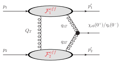
Figure 1: Generic diagram for the Durham model approach to the considered exclusive production processes.

Recently our group showed how to include relativistic corrections for the inclusive production of $\eta_{c}$ BPSS2019 and very recently for inclusive production of $\chi_{c0}$ BPSS2020 using the light-cone wave functions of the charmonia derived from the well-known $c\bar{c}$ interquark potential models. It is the aim of the present paper to do a similar study for the exclusive case. In addition, there is no such a study on the $pp\to pp\eta_{c}$ CEP available in the literature. In contrast, inclusive production of $\eta_{c}(1S)$ was measured by the LHCb collaboration in proton-proton collisions for $\sqrt{s}$ = 7, 8, 13 TeV LHCb . Is such a measurement possible for the exclusive production of $\eta_{c}$? This study is a first step to address this important question. An analysis of inclusive diffractive production of $\eta_{c}(1S)$ was done recently in Tichouk:2020dut .

In the present paper, we wish to discuss in parallel the exclusive production process of both the scalar $\chi_{c0}$ and pseudoscalar $\eta_{c}$ quarkonia For illustration of the corresponding production mechanism initially proposed by the Durham group KMR , see Fig. 1. We start with a brief introduction into the formalism for $pp\to p\,\chi_{c0}\,p$ and $pp\to p\,\eta_{c}\,p$ reactions based upon the Durham model of CEP KMR setting up the necessary notation and conventions. In this model, a quarkonium state is produced via fusion of two virtual active gluons accompanied by an extra exchange with a screening gluon as is shown in Fig. 1. The additional exchange of the gluon provides colour conservation and hence the effective color singlet exchange in the $t$-channel. As a result, in the final state, in addition to the meson produced mainly at central rapidities, there are two forward protons that retain most of their initial energy. We intend to calculate the integrated cross sections for such processes as well as several differential distributions relevant for future measurements. We wish to discuss both the hard and soft processes involved in these reactions in the light-front QCD approach, to consider several prescriptions on how to calculate the off-diagonal UGDs (some of them have already been used previously in the literature) and to estimate the absorptive corrections in the differential distributions.

II Virtual gluon fusion into pseudo(scalar) charmonia

Below, we shall consider the hard $\chi_{c0}(1P)$ and $\eta_{c}(1S)$ charmonia production subprocesses separately.

II.1 The light-cone amplitude for $g^{*}g^{*}\to\chi_{c0}(1P)$ process

The gluon-gluon fusion vertex is proportional to the reduced amplitude ${\cal T}_{\mu\nu}$ as follows:

$${\cal V}^{ab}_{\mu\nu}(g^{*}g^{*}\to\chi_{c0}) = 4\pi\alpha_{s}{{\mbox{\rm Tr}}[t^{a}t^{b}]\over\sqrt{N_{c}}}\,2{\cal T}_{\mu\nu}={4\pi\alpha_{s}\over\sqrt{N_{c}}}\,\delta^{ab}{\cal T}_{\mu\nu}\,,$$ (1)

$${\cal T}_{\mu\nu}=-\delta^{\perp}_{\mu\nu}(q_{1},q_{2})G_{\rm TT}(q_{1}^{2},q_{2}^{2})\,+e_{\mu}^{L}(q_{1})e_{\nu}^{L}(q_{2})G_{\rm LL}(q_{1}^{2},q_{2}^{2})\,,$$ (2)

where $\alpha_{s}$ is the strong coupling, $N_{c}=3$ and $t^{a}$ are the number of colors and $SU(3)$ group generators in QCD, respectively, and

$$\left(\begin{array}[]{c}G_{\rm TT}\\ G_{\rm LL}\end{array}\right) = \begin{pmatrix}-|\mbox{\boldmath$q$}_{1}||\mbox{\boldmath$q$}_{2}|&(q_{1}\cdot q_{2})\\ (q_{1}\cdot q_{2})&-|\mbox{\boldmath$q$}_{1}||\mbox{\boldmath$q$}_{2}|\end{pmatrix}\;\left(\begin{array}[]{c}G_{1}\\ G_{2}\end{array}\right)\;,$$ (7)

while the relevant kinematical variables are displayed in Fig. 1. Here, we have the projector on transverse polarization states

$$-\delta^{\perp}_{\mu\nu}(q_{1},q_{2})=-g_{\mu\nu}+{1\over X}\Big{(}(q_{1}\cdot q_{2})(q_{1\mu}q_{2\nu}+q_{1\nu}q_{2\mu})-q_{1}^{2}q_{2\mu}q_{2\nu}-q_{2}^{2}q_{1\mu}q_{1\nu}\Big{)}\,,$$ (9)

with $X=(q_{1}\cdot q_{2})^{2}-q_{1}^{2}q_{2}^{2}$. The longitudinal polarization vectors read as follows

$$e_{\mu}^{L}(q_{1}) = \sqrt{{-q_{1}^{2}\over X}}\Big{(}q_{2\mu}-{q_{1}\cdot q_{2}\over q_{1}^{2}}q_{1\mu}\Big{)}\,,\qquad e_{\nu}^{L}(q_{2})=\sqrt{{-q_{2}^{2}\over X}}\Big{(}q_{1\nu}-{q_{1}\cdot q_{2}\over q_{2}^{2}}q_{2\nu}\Big{)}\,.$$ (10)

The convoluted form of reduced amplitude can be written as

$${\cal T}=n^{+}_{\nu}n^{-}_{\mu}{\cal T_{\mu\nu}}=|\mbox{\boldmath$q$}_{1}||\mbox{\boldmath$q$}_{2}|G_{1}(q_{1}^{2},q_{2}^{2})+(\mbox{\boldmath$q$}_{1}\cdot\mbox{\boldmath$q$}_{2})G_{2}(q_{1}^{2},q_{2}^{2})\,,$$ (11)

in terms of the light cone vectors $n^{\pm}_{\nu}=(1,0,0,\pm 1)$. The form factors here $G_{i}(\mbox{\boldmath$q$}_{1}^{2},\mbox{\boldmath$q$}_{2}^{2})$ have the integral representations in terms of the $P$-wave charmonia wave function $\psi_{\chi}(z,\mbox{\boldmath$k$})$ (see Ref. BPSS2020 for more details)

$$G_{1}(\mbox{\boldmath$q$}_{1}^{2},\mbox{\boldmath$q$}_{2}^{2}) = |\mbox{\boldmath$q$}_{1}||\mbox{\boldmath$q$}_{2}|\,{4m_{c}\over\mbox{\boldmath$q$}_{2}^{2}}\int{dzd^{2}\mbox{\boldmath$k$}\over z(1-z)16\pi^{3}}\psi_{\chi}(z,\mbox{\boldmath$k$})\,2z(1-z)(2z-1)\Big{[}{1\over\mbox{\boldmath$l$}_{A}^{2}+\varepsilon^{2}}-{1\over\mbox{\boldmath$l$}_{B}^{2}+\varepsilon^{2}}\Big{]}$$

$$G_{2}(\mbox{\boldmath$q$}_{1}^{2},\mbox{\boldmath$q$}_{2}^{2}) = 4m_{c}\int{dzd^{2}\mbox{\boldmath$k$}\over z(1-z)16\pi^{3}}\psi_{\chi}(z,\mbox{\boldmath$k$})\Big{[}{1-z\over\mbox{\boldmath$l$}_{A}^{2}+\varepsilon^{2}}+{z\over\mbox{\boldmath$l$}_{B}^{2}+\varepsilon^{2}}\Big{]}$$ (12)

$$+ {4m_{c}\over\mbox{\boldmath$q$}_{2}^{2}}\int{dzd^{2}\mbox{\boldmath$k$}\over z(1-z)16\pi^{3}}\psi_{\chi}(z,\mbox{\boldmath$k$})4z(1-z)\Big{[}{\mbox{\boldmath$q$}_{2}\cdot\mbox{\boldmath$l$}_{A}\over\mbox{\boldmath$l$}_{A}^{2}+\varepsilon^{2}}-{\mbox{\boldmath$q$}_{2}\cdot\mbox{\boldmath$l$}_{B}\over\mbox{\boldmath$l$}_{B}^{2}+\varepsilon^{2}}\Big{]}\,,$$

where $z$ is a $c$-quark (or $\bar{c}$-antiquark) momentum fraction, $k$ is the relative $c\bar{c}$ transverse momentum, $m_{c}$ is the mass of $c$-quark, and the shorthand notations

$$\varepsilon^{2} = z(1-z)\mbox{\boldmath$q$}_{1}^{2}+m_{c}^{2}\,,\qquad\mbox{\boldmath$l$}_{A}=\mbox{\boldmath$k$}-(1-z)\mbox{\boldmath$q$}_{2}\,,\qquad\mbox{\boldmath$l$}_{B}=\mbox{\boldmath$k$}+z\mbox{\boldmath$q$}_{2}\,,$$ (13)

have been introduced.

II.2 The light cone amplitude for $g^{*}g^{*}\to\eta_{c}$ process

In Ref. BPSS2019 , we introduced the covariant form of the vertex for two off-shell gluon fusion into $\eta_{c}$ meson:

$${\cal V}^{ab}_{\mu\nu}=(-i)4\pi\alpha_{s}\epsilon_{\mu\nu\alpha\beta}q^{\alpha}q^{\beta}{\delta^{ab}\over 2\sqrt{N_{c}}}2I(\mbox{\boldmath$q$}_{1}^{2},\mbox{\boldmath$q$}_{2}^{2})\,,$$ (14)

where $I(\mbox{\boldmath$q$}_{1}^{2},\mbox{\boldmath$q$}_{2}^{2})=F_{\gamma^{*}\gamma^{*}\to\eta_{c}}(\mbox{\boldmath$q$}_{1}^{2},\mbox{\boldmath$q$}_{2}^{2})/(e^{2}_{c}\sqrt{N_{c}}$), or in the convoluted form:

$${\cal V}^{ab}=(-i)4\pi\alpha_{s}{\delta^{ab}\over\sqrt{N_{c}}}I(\mbox{\boldmath$q$}_{1}^{2},\mbox{\boldmath$q$}_{2}^{2})|\mbox{\boldmath$q$}_{1}||\mbox{\boldmath$q$}_{2}|\sin(\phi_{1}-\phi_{2})\,,$$ (15)

with $(\phi_{1}-\phi_{2})$ being the angle between $\mbox{\boldmath$q$}_{1}$ and $\mbox{\boldmath$q$}_{2}$. We then express $I(\mbox{\boldmath$q$}_{1}^{2},\mbox{\boldmath$q$}_{2}^{2})$ in terms of light-cone wave functions as follows Babiarz:2019sfa

$$I(\mbox{\boldmath$q$}_{1}^{2},\mbox{\boldmath$q$}_{2}^{2}) = 4m_{c}\int{dzd^{2}\mbox{\boldmath$k$}\over z(1-z)16\pi^{3}}\psi_{\eta}(z,\mbox{\boldmath$k$})\Big{\{}{1-z\over(\mbox{\boldmath$k$}-(1-z)\mbox{\boldmath$q$}_{2})^{2}+z(1-z)\mbox{\boldmath$q$}_{1}^{2}+m_{c}^{2}}$$ (16)

$$+ {z\over(\mbox{\boldmath$k$}+z\mbox{\boldmath$q$}_{2})^{2}+z(1-z)\mbox{\boldmath$q$}_{1}^{2}+m_{c}^{2}}\Big{\}}\,,$$

where $\psi_{\eta}(z,\mbox{\boldmath$k$})$ is the wave function of $\eta_{c}(1S)$ meson.

III Matrix element for $pp\to ppM$ reaction

The amplitude for the CEP process for a given meson $V\equiv\chi_{c0},\,\eta_{c}$ reads:

$${\cal M} = {s\over 2}\pi^{2}{1\over 2}{\delta_{c_{1}c_{2}}\over N_{c}^{2}-1}\int d^{2}\mbox{\boldmath$Q$}\;{\cal V}^{c_{1}c_{2}}{{\cal F}_{g}^{\rm off}(x_{1},x^{\prime},\mbox{\boldmath$Q$}^{2},\mbox{\boldmath$q$}_{1}^{2},\mu^{2},t_{1}){\cal F}_{g}^{\rm off}(x_{2},x^{\prime},\mbox{\boldmath$Q$}^{2},\mbox{\boldmath$q$}_{2}^{2},\mu^{2},t_{2})\over\mbox{\boldmath$Q$}^{2}\mbox{\boldmath$q$}_{1}^{2}\mbox{\boldmath$q$}_{2}^{2}}\,,$$ (17)

in terms of the “active” (fusing into $V$) $x_{1,2}$ and “screening” $x^{\prime}$ (connecting both proton lines) gluon momentum fractions. The screening gluon carries a transverse momentum $Q$, while the transverse momenta of active gluons are denoted by $\mbox{\boldmath$q$}_{1},\mbox{\boldmath$q$}_{2}$. The generalized unintegrated gluon distributions (UGDs) also depend on the hard scale of the process $\mu$ (see below). The $2\to 3$ total cross section can be calculated generically as follows:

$$\sigma = {1\over 2s}\int|{\cal M}|^{2}(2\pi)^{4}\delta^{4}(p_{1}+p_{2}-p_{1}^{\prime}-p_{2}^{\prime}-p_{V})$$ (18)

$$\times \Big{(}{1\over 2(2\pi)^{3}}\Big{)}^{3}(dy_{1}^{\prime}d^{2}\mbox{\boldmath$p$}_{1}^{\prime})(dy_{2}^{\prime}d^{2}\mbox{\boldmath$p$}_{2}^{\prime})(dyd^{2}\mbox{\boldmath$p$}_{V})\,,$$

or, following a simplification done in Ref. Szczurek:2006bn , as

$$\sigma={1\over 2s}{1\over 2^{8}\pi^{4}s}\int|{\cal M}|^{2}dt_{1}dt_{2}dyd\phi\,.$$ (19)

Above, $t_{1}=(p_{1}-p_{1}^{\prime})^{2}$, $t_{2}=(p_{2}-p_{2}^{\prime})^{2}$ and $\phi\in(0,2\pi)$ is the relative azimuthal angle between the outgoing protons, $s$ is the $pp$ center-of-mass energy squared, $y$ is rapidity of the outgoing meson $V$.

IV Different approaches to off-diagonal gluon densities

In the forward limit of small $t_{1,2}\to 0$ corresponding to $\mbox{\boldmath$Q$}^{2}\simeq\mbox{\boldmath$q$}_{1,2}^{2}\equiv Q_{\perp}^{2}$, the generalized UGDs in Eq. (17) are simplified and are considered as functions of only one transverse momentum, i.e.

$${\cal F}_{g}^{\rm off}(x_{1},x^{\prime},\mbox{\boldmath$Q$}^{2},\mbox{\boldmath$q$}_{1}^{2},\mu^{2},t_{1})\to{\cal F}_{g}^{\rm off}(x_{1},x^{\prime},Q_{\perp}^{2},\mu^{2},t_{1})\,.$$ (20)

The Khoze-Martin-Ryskin (KMR) prescription for the off-diagonal (“skewed”) UGD includes a Sudakov form factor $T_{g}(q_{\perp}^{2},\mu^{2})$ and is typically written as KMR

$${\cal F}_{g,{\rm KMR}}^{\rm off}(x,x^{\prime},Q_{\perp}^{2},\mu^{2};t)=R_{g}{d\over{d{\rm ln}}q_{\perp}^{2}}\Big{[}xg(x,q_{\perp}^{2})\sqrt{T_{g}(q_{\perp}^{2},\mu^{2})}\Big{]}_{q_{\perp}^{2}=Q_{\perp}^{2}}F(t)\,,$$ (21)

with gluon virtualities $q_{\perp}^{2}\equiv\mbox{\boldmath$q$}^{2}$ playing a role of the momentum scale squared in the collinear gluon density $xg(x,q_{\perp}^{2})$, and with the nucleon form factor $F(t)$ often parameterised in the following two ways

$$F(t)={4m_{p}^{2}-2.79t\over(4m_{p}^{2}-t)(1-t/0.71)^{2}}\qquad{\rm or}\qquad F(t)=\exp\Big{(}{bt\over 2}\Big{)}\,,\quad b=4\,{\rm GeV}^{-2}\,,$$ (22)

with $m_{p}$ being the proton mass, corresponding to the isoscalar nucleon form factor Donnachie:1987pu or the QCD elastic profile factor, respectively.

The Sudakov form factor is taken as:

$$T_{g}(q_{\perp}^{2},\mu^{2})=\exp\Big{[}-\int_{q_{\perp}^{2}}^{\mu^{2}}{{d\mbox{\boldmath$k$}_{\perp}^{2}\over\mbox{\boldmath$k$}_{\perp}^{2}}{\alpha_{s}(k_{\perp}^{2})\over 2\pi}}\int_{0}^{1-\Delta}{\Big{[}zP_{gg}(z)+\sum_{q}P_{qg}(z)\Big{]}dz}\Big{]},$$ (23)

with the hard scale $\mu^{2}=M^{2}_{V}+q_{\perp}^{2}\,$ and $\Delta=k_{\perp}/(k_{\perp}+\mu)$.

Regarding the longitudinal momentum fractions, central diffractive production is dominated by the region $x^{\prime}\ll x_{1,2}\ll 1$. We thus compute the skewedness correction $R_{g}$ in Eq. (21) using a method proposed and derived for the collinear off-diagonal gluon distributions Shuvaev:1999ce :

$$R_{g}={2^{2\lambda+3}\over\sqrt{\pi}}{\Gamma(\lambda+5/2)\over\Gamma(\lambda+4)}\,,\qquad\lambda={d\over d{\rm ln}(1/x)}\Big{[}{\rm ln}\Big{(}xg(x,q_{\perp}^{2})\Big{)}\Big{]}\,.$$ (24)

In a slightly off-forward case $t_{1,2}\not=0$, the choice of $Q_{\perp}$ in the off-diagonal KMR gluon in Eq. (21) becomes somewhat arbitrary. In practical calculations, we use the so-called “minimum prescription” proposed by the Durham group, by substituting $Q^{2}_{\perp}~{}\to{\rm min}(Q^{2}_{\perp},q^{2}_{\perp})$ in Eq. (21), with transverse momentum of an active gluon $q_{\perp}$ and transverse momentum of the screening gluon $Q_{\perp}$. In addition, we suggest a geometrical average of active and screening gluon momenta as $Q^{2}_{\perp}\to\sqrt{Q^{2}_{\perp}q^{2}_{\perp}}$ – an option, called BPSS in the following, for brevity.

We vary our results by also using the modified off-diagonal CDHI gluon defined as Cudell:2008gv

$${\cal F}^{\rm off}_{g,{\rm CDHI}}(x,x^{\prime},Q_{\perp},\mu^{2};t)=R_{g}\Big{[}{\partial\over\partial\log\bar{Q}^{2}}\sqrt{T_{g}(\bar{Q}^{2},\mu^{2})}\,xg(x,\bar{Q}^{2})\Big{]}\cdot{2Q_{\perp}^{2}q_{\perp}^{2}\over Q_{\perp}^{4}+q_{\perp}^{4}}\cdot F(t)\,,$$ (25)

where $\bar{Q}^{2}=(Q^{2}_{\perp}+q^{2}_{\perp})/2$. In order to take into account the saturation effects, we use of the simplest saturation-based UGD inspired by the Golec-Biernat-Wüsthoff (GBW) model GolecBiernat:1999qd . In order to extrapolate it into the off-diagonal domain, we use the prescription proposed in Ref. Pasechnik:2007hm (further referred to as the PST prescription):

$${\cal F}^{\rm off}_{g,{\rm GBW}}=\sqrt{Q_{\perp}^{2}f^{\rm GBW}_{g}(x^{\prime},Q_{\perp}^{2})q_{\perp}^{2}f^{\rm GBW}_{g}(x,q_{\perp}^{2})}\,\sqrt{T_{g}(q_{\perp}^{2},\mu^{2})}\,F(t)\,,$$ (26)

$$f^{\rm GBW}_{g}(x,q_{\perp}^{2})={3\,\sigma_{0}\over 4\pi^{2}\alpha_{s}}R_{0}^{2}\,q_{\perp}^{2}\exp[R_{0}^{2}\,q_{\perp}^{2}]\,,$$

where $f^{\rm GBW}_{g}$ is the diagonal GBW UGD, and $x^{\prime}=|\mbox{\boldmath$Q$}|/\sqrt{s}$, $R_{0}=(x/x_{0})^{\lambda/2}$. In practical calculations, we have used the following fitted values of the GBW parameters obtained by Golec-Biernat and Sapeta Golec-Biernat:2017lfv : $\sigma_{0}=29.12$ mb, $\lambda=0.277$, $x_{0}/10^{-4}=0.41$, with $\alpha_{s}(q_{\perp}^{2})={\rm min}(0.82,{4\pi\over 9\log(Q^{2}/\Lambda^{2}_{\rm QCD})})$ and $Q^{2}={{\rm max}}(q_{\perp}^{2},0.22\,{\rm GeV}^{2})$, $\Lambda_{\rm QCD}^{2}=0.04\,{\rm GeV}^{2}$.

As an alternative model based on the color dipole cross section, we used a fit obtained by Rezaeian and Schmidt Rezaeian:2013tka . While the GBW model resembles the eikonal unitarization, the Rezaeian-Schmidt cross section uses a form of the dipole cross section proposed in Ref. Iancu:2003ge which is motivated by the BFKL equation and its nonlinear generalizations. We computed the corresponding UGD $f^{\rm RS}_{g}(x,|\mbox{\boldmath$q$}|)$ as

$$f^{RS}_{g}(x,|\mbox{\boldmath$q$}|)=\mbox{\boldmath$q$}^{2}{\sigma_{0}\over\alpha_{s}}{N_{c}\over 8\pi^{2}}\int_{0}^{\infty}rdr\,J_{0}(|\mbox{\boldmath$q$}|r)\Big{(}1-{\sigma(x,r)\over\sigma_{0}}\Big{)}\,.$$ (27)

As an example, we have used the first set of parameters from Table I in Ref. Rezaeian:2013tka .

V Numerical results

In the CEP processes at high energies, it is mandatory to consider gluons carrying very small longitudinal momentum fractions $x$. For this purpose, in practical calculations we use a few parton distribution functions (PDFs): JR14NLO JR14 ($Q_{0T}^{2}=0.8\,{\rm GeV}^{2}$), GJR08NLO GJR08 ($Q_{0T}^{2}=0.5\,{\rm GeV}^{2}$) and GRV94NLO GRV ($Q_{0T}^{2}=0.4\,{\rm GeV}^{2}$). In Fig. 2, we illustrate the shape of the corresponding gluon PDFs at scales and longitudinal momenta fractions typical for the considered $pp\to pp\eta_{c}$ and $pp\to pp\chi_{c,0}$ CEP processes. In the range of scales under discussion, the gluon PDFs from the literature differ considerably. We do not employ the Durham or CTEQ PDFs for which the initial scales for evolution are rather high making them difficult to be applied in the context of the exclusive reactions discussed here.

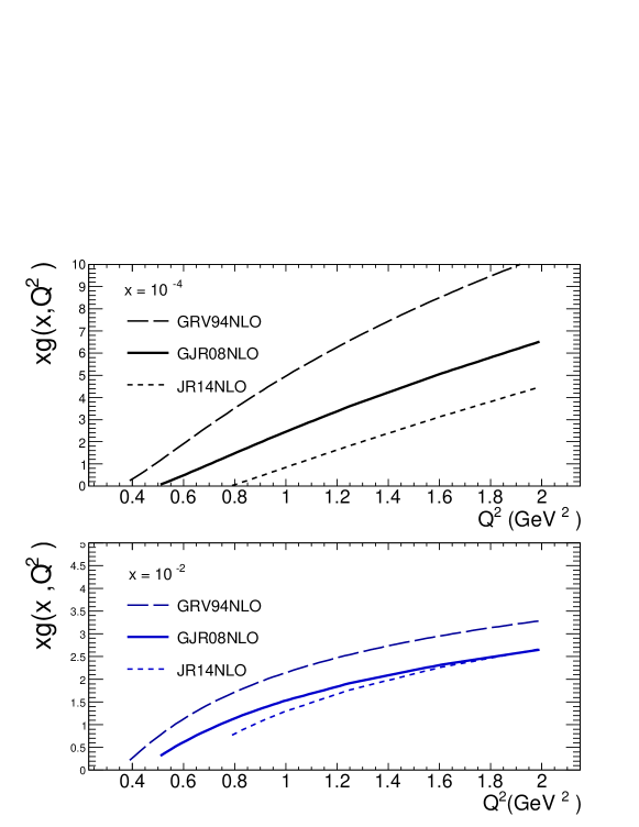
Figure 2: Collinear gluon PDF as a function of the hard scale of the process and for typical longitudinal gluon momentum fractions, $x=10^{-4}$ (upper plot) and $x=10^{-2}$ (lower plot).

The total cross sections computed over the full phase space for each PDF mentioned above are listed in Tables 1 and 2, for $\chi_{c0}$ and $\eta_{c}$, respectively. The integrated cross section for $pp\to pp\chi_{c0}$ at $\sqrt{s}=$ 13 TeV is shown in Table 1 for different off-diagonal UGD prescriptions for the effective $Q_{iT}^{2}$ summarized as follows:

• (a) Durham prescription (Eq. (21)): $Q_{iT}^{2}=\min(Q_{T}^{2},q_{iT}^{2})$  ,

• (b) BPSS prescription (Eq. (21)): $Q_{iT}^{2}=\sqrt{Q_{T}^{2}q_{iT}^{2}}$  ,

• (c) CDHI prescription (Eq. (25)): $Q_{iT}^{2}=(Q_{T}^{2}+q_{iT}^{2})/2$  ,

• (d) PST off-diagonal UGD (Eq. (26))  .

For $\chi_{c}$ production, these prescriptions lead to similar cross sections of the order of 1 $\mu$b before including absorption effects. The corresponding gap survival factor is of the order of 0.1 as will be discussed at the end of this section.

Table 1: Total cross section for $\chi_{c0}$ at $\sqrt{s}=13\,{\rm TeV}$ with $R_{g}=1.0$ and $R_{g}$ according to Eq. (24). In order to obtain the cross section, several gluon distributions were used with $Q_{0T}^{2}\geq 0.4\,{\rm GeV}^{2}$ for GRV94NLO, $Q_{0T}^{2}\geq 0.5\,{\rm GeV}^{2}$ for GJR08NLO, and $Q_{0T}^{2}\geq 0.8\,{\rm GeV}^{2}$ for JR14NLO. The light-cone form factor for the $gg\to\chi_{c0}$ coupling was calculated using the Buchmüller-Tye potential (for more details, see Ref. BPSS2020 ) No gap survival factor is included here.

KMR Skewed gluon $0.8\,{\rm GeV}^{2}\leq Q_{0T}^{2}$, JR14NLO	$\sigma_{\rm tot}$ [nb], $R_{g}=1.0$	$\sigma_{\rm tot}$ [nb], $R_{g}(x,Q_{iT}^{2})$
CDHI, $Q_{iT}^{2}=(Q_{T}^{2}+q_{iT}^{2})/2.$	$0.42\cdot 10^{3}$	$1.1\cdot 10^{3}$
KMR, $Q_{iT}^{2}=\sqrt{Q_{T}^{2}\cdot q_{iT}^{2}}$	$0.36\cdot 10^{3}$	$0.94\cdot 10^{3}$
KMR, $Q_{iT}^{2}=\min(Q_{T}^{2},q_{iT}^{2})$	$0.20\cdot 10^{3}$	$0.52\cdot 10^{3}$
KMR Skewed gluon $0.5\,{\rm GeV}^{2}\leq Q_{0t}^{2}$, GJR08NLO	$\sigma_{\rm tot}$ [nb], $R_{g}=1.0$	$\sigma_{\rm tot}$ [nb], $R_{g}(x,Q_{iT}^{2})$
CDHI, $Q_{iT}^{2}=(Q_{T}^{2}+q_{iT}^{2})/2.$	$0.46\cdot 10^{3}$	$1.57\cdot 10^{3}$
KMR, $Q_{iT}^{2}=\sqrt{Q_{T}^{2}\cdot q_{iT}^{2}}$	$0.64\cdot 10^{3}$	$2.1\cdot 10^{3}$
KMR, $Q_{iT}^{2}=\min(Q_{T}^{2},q_{iT}^{2})$	$0.34\cdot 10^{3}$	$1.1\cdot 10^{3}$
KMR Skewed gluon $0.4\,{\rm GeV}^{2}\leq Q_{0T}^{2}$, GRV94NLO	$\sigma_{\rm tot}$ [nb], $R_{g}=1.0$	$\sigma_{\rm tot}$ [nb], $R_{g}(x,Q_{iT}^{2})$
CDHI, $Q_{iT}^{2}=(Q_{T}^{2}+q_{iT}^{2})/2.$	$1.88\cdot 10^{3}$	$9.02\cdot 10^{3}$
KMR, $Q_{iT}^{2}=\sqrt{Q_{T}^{2}\cdot q_{iT}^{2}}$	$3.03\cdot 10^{3}$	$13.4\cdot 10^{3}$
KMR, $Q_{iT}^{2}=\min(Q_{T}^{2},q_{iT}^{2}),0.4{\rm GeV}^{2}\leq Q_{0T}^{2}$	$1.4\cdot 10^{3}$	$6.1\cdot 10^{3}$
KMR, $Q_{iT}^{2}=\min(Q_{T}^{2},q_{iT}^{2}),0.8{\rm GeV}^{2}\leq Q_{0T}^{2}$	$0.75\cdot 10^{3}$	$3.9\cdot 10^{3}$
PST Skewed gluon	$\sigma_{\rm tot}$ [nb]	-
PST prescription, GBW	$0.44\cdot 10^{3}$	-
PST prescription, RS	$0.52\cdot 10^{3}$	-

In Table 2 we present similar results for $\eta_{c}$ production. The total cross section for the $\eta_{c}$ production is 3-4 orders of magnitude smaller than that for $\chi_{c0}$, i.e. surprisingly small. The cross section for the PST prescription for off-diagonal gluon is quite similar as for the Durham and CDHI prescriptions in the case of $\chi_{c0}$, while the spread in the total cross section for $\eta_{c}$ is much higher.

Table 2: The same as in Table 1 but for the $\eta_{c}$ meson. The light-cone form factor for the $gg\to\eta_{c}(1S)$ coupling was calculated using the power-law potential (for more details, see Ref. BPSS2019 ).

KMR Skewed gluon, $0.8{\rm GeV}^{2}\leq Q_{0T}^{2}$, JR14NLO	$\sigma_{\rm tot}$ [nb], $R_{g}=1.0$	$\sigma_{\rm tot}$ [nb], $R_{g}(x,Q_{iT}^{2})$
CDHI, $Q_{iT}^{2}=(Q_{T}^{2}+q_{iT}^{2})/2.$	$1.1$	$2.4$
KMR, $Q_{iT}^{2}=\sqrt{Q_{T}^{2}\cdot q_{iT}^{2}}$	$0.39$	$1.2$
KMR, $Q_{iT}^{2}=\min(Q_{T}^{2},q_{iT}^{2})$	$0.13$	$0.25$
KMR Skewed gluon, $0.5{\rm GeV}^{2}\leq Q_{0T}^{2}$, GJR08NLO	$\sigma_{\rm tot}$ [nb], $R_{g}=1.0$	$\sigma_{\rm tot}$ [nb], $R_{g}(x,Q_{iT}^{2})$
CDHI, $Q_{iT}^{2}=(Q_{T}^{2}+q_{iT}^{2})/2.$	$2.2$	$5.6$
KMR, $Q_{iT}^{2}=\sqrt{Q_{T}^{2}\cdot q_{iT}^{2}}$	$0.52$	$2.1$
KMR, $Q_{iT}^{2}=\min(Q_{T}^{2},q_{iT}^{2}),0.5{\rm GeV}^{2}\leq Q_{0T}^{2}$	$0.44$	$1.3$
KMR, $Q_{iT}^{2}=\min(Q_{T}^{2},q_{iT}^{2}),0.8{\rm GeV}^{2}\leq Q_{0T}^{2}$	$0.22$	$0.45$
KMR Skewed gluon, $0.4{\rm GeV}^{2}\leq Q_{0T}^{2}$, GRV94NLO	$\sigma_{\rm tot}$ [nb], $R_{g}=1.0$	$\sigma_{\rm tot}$ [nb], $R_{g}(x,Q_{iT}^{2})$
CDHI, $Q_{iT}^{2}=(Q_{T}^{2}+q_{iT}^{2})/2.$	$1.2\cdot 10^{2}$	$7.8\cdot 10^{3}$
KMR, $Q_{iT}^{2}=\sqrt{Q_{T}^{2}\cdot q_{iT}^{2}}$	$2.2$	$1.3\cdot 10^{3}$
KMR, $Q_{iT}^{2}=\min(Q_{T}^{2},q_{iT}^{2}),0.4{\rm GeV}^{2}\leq Q_{0T}^{2}$	$2.8$	$1.0\cdot 10^{1}$
KMR, $Q_{iT}^{2}=\min(Q_{T}^{2},q_{iT}^{2}),0.8{\rm GeV}^{2}\leq Q_{0T}^{2}$	$1.25$	$2.9$
PST Skewed gluon	$\sigma_{\rm tot}$ [nb]	-
PST, GBW	$1.9$	-
PST, RS	$4.1$

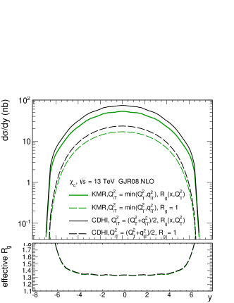
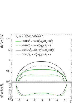
Figure 3: The rapidity distribution for $\chi_{c0}$, $\eta_{c}$ quarkonia CEP and effective $R_{g}$ factor calculated with the GJR08NLO parton distribution function. No gap survival factor is included here.

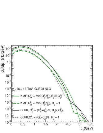
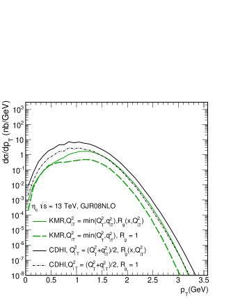
Figure 4: Distribution in transverse momentum of the $\chi_{c0}$ (left) and $\eta_{c}$ (right) quarkonia CEP, respectively, with different treatment of $R_{g}$ factor. No gap survival factor is included here.

In Fig. 3 we show the rapidity distribution of $\chi_{c,0}$ (left) and $\eta_{c}$ (right) quarkonia CEP. We show results for the Durham (min) and CDHI prescription for the off-diagonal UGDFs. We present results for $R_{g}=$ 1 as well as with $R_{g}$ calculated according to the Shuvaev prescription (see Eq. (24)). Inclusion of $R_{g}$ increases the cross section by a factor of 3-4. While for $\chi_{c0}$ the difference of the results for the Durham prescription and the CDHI prescription is small, for $\eta_{c}$ the difference is of the order of magnitude size.

The distribution in transverse momentum are shown in Fig. 4. The distribution for $\eta_{c}$ and $\chi_{c0}$ CEP are somewhat different. The maximum of the cross-section for $\eta_{c}$ is at $p_{T}\sim 1\,{\rm GeV}$ and the dip at vanishing $p_{T}$ is more pronounced.

In Fig. 5 we show two-dimensional distributions in $(t_{1},t_{2})$ ($t_{1}$, $t_{2}$ are four-momenta squared transferred in the proton lines), for $pp\to pp\eta_{c}(1S)$ CEP process at $\sqrt{s}=13\,{\rm TeV}$. Here, we present results for several prescriptions for the off-diagonal KMR UGDFs: with the Durham prescription – left-upper panel, the BPSS prescription – right-upper panel, and the CDHI prescription – left-lower panel as well as the PST prescription for off-diagonal UGD using the diagonal GBW UGDF – right-lower panel. No gap survival effect is incorporated here. The results appear to be reasonably stable with respect to a change in the UGDs modelling, while the BPSS prescription differ in the distribution shape.

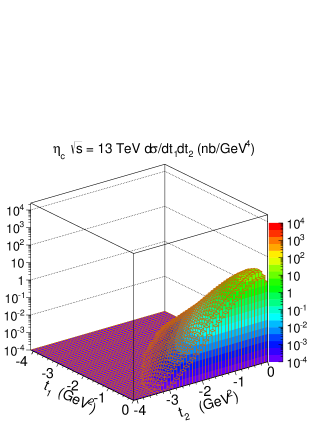
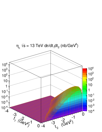
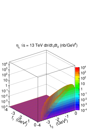
Figure 5: Distribution in $t_{1}\times t_{2}$ for CDHI (left-upper), BPSS (right-upper) and Durham (left-lower) prescriptions calculated with the GJR08NLO gluon distribution function and for the PST off-diagonal UGD computed with the diagonal GBW UGD (right-lower) for $\eta_{c}$ CEP for $\sqrt{s}=13\,{\rm TeV}$. No gap survival factor is included here.

For completeness, in Fig. 6 we show similar results for the $\chi_{c0}$ production. In this case, all prescriptions for effective transverse momenta (Durham, BPSS, and CDHI prescriptions) lead to fairly similar results. Here the cross sections are peaked at $t_{1}$ = 0, $t_{2}$ = 0.

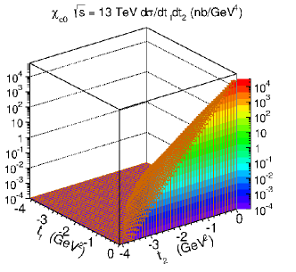
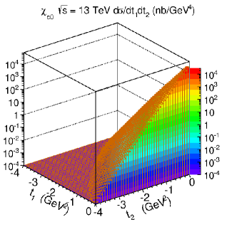
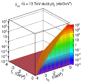
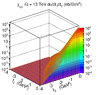
Figure 6: Distribution in $t_{1}\times t_{2}$ for CDHI (left-upper), BPSS ($Q_{iT}^{2}=\sqrt{q_{iT}^{2},Q_{T}^{2}}$) (right-upper) and Durham ($Q^{2}_{iT}=\min(q^{2}_{iT},Q^{2}_{T})$) (left-lower) prescriptions calculated with the GJR08NLO gluon distribution function and for the PST off-diagonal UGD computed with the diagonal GBW UGD (right-lower) for $\chi_{c0}$ for $\sqrt{s}=13\,{\rm TeV}$. No gap survival factor is included here.

In Fig. 7 we show relative azimuthal angle (between outgoing protons) distributions. The distribution for $\chi_{c0}$ (left) is very different than that for $\eta_{c}$ (right). While for $\chi_{c0}$ there is one maximum for the back-to-back configurations, there are two maxima for $\eta_{c}$. The cross section vanishes in the back-to-back kinematics in the case of $\eta_{c}$ CEP. The exact position of the maxima depends on the details of the treatment of the off-diagonal UGDs so their experimental identification could pin down the correct theoretical modelling of these objects.

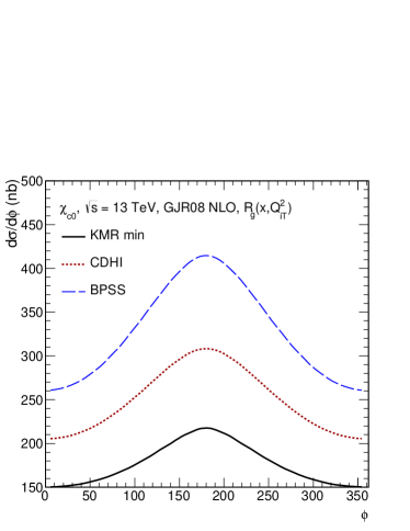
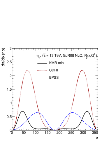
Figure 7: Distribution in relative azimuthal angle between outgoing protons, for $\chi_{c0}$ – left panel, and for $\eta_{c}$ – right panel, using different prescriptions for UGDs. No gap survival factor is included here.

Finally, we wish to compare our results for the exclusive reactions $pp\to pp\eta_{c}$ and $pp\to pp\chi_{c0}$ with their inclusive production counterparts as calculated recently in Refs. BPSS2019 and BPSS2020 . In Figs. 8 and 9 we show the numerical results (rapidity and transverse momentum distributions) for $\eta_{c}$ and $\chi_{c0}$, respectively. While for $\eta_{c}$ production the cross section for the exclusive process is a few orders of magnitude lower than that for the inclusive case, this is quite different for $\chi_{c0}$ meson. Both for rapidity and transverse momentum distributions the results for the exclusive case are very different compared to the inclusive case.

The two UGDs obtained from the dipole cross section, labelled GBW and RS, give rise to similar distributions. For the case of $\eta_{c}$ the RS UGD gives a larger cross section than that obtained with the GBW model, while in the case of $\chi_{c}$ their sizes are very similar.

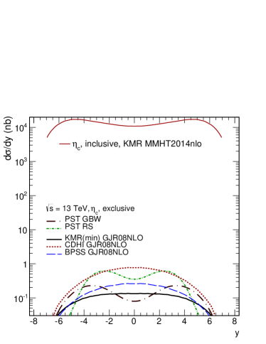
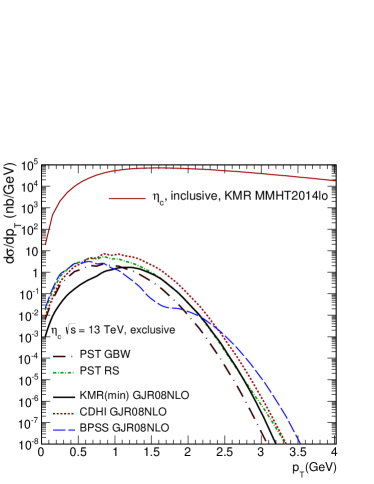
Figure 8: Comparison of exclusive and inclusive $\eta_{c}$ production at $\sqrt{s}=13\,{\rm TeV}$. No gap survival factor is included for the exclusive reaction.

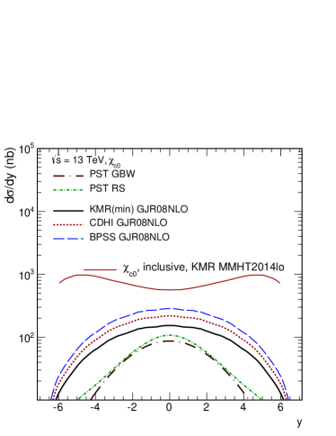
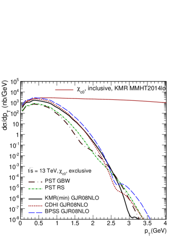
Figure 9: Comparison of exclusive and inclusive $\chi_{c0}$ production at $\sqrt{s}=13\,\rm{TeV}$. No gap survival factor is included for the exclusive reaction.

VI Absorptive corrections

It is understood that the Born-level cross sections receive absorptive corrections through hadronic rescatterings at large distances. These are related to the interactions of spectator partons Bjorken:1992er . They give rise to the so-called gap survival probability in exclusive reactions. The calculation of the latter poses a difficult problem, which has not been solved yet in a way fully consistent with the perturbative QCD approach to the production amplitude.

Numerous approaches exist in the literature, some of them are based on soft multi-Pomeron exchanges Gotsman:1999xq ; Kaidalov:2001iz ; Ostapchenko:2017prv , while other approaches avoid the decomposition into Born term and absorptive correction altogether treating the absorptive effects dynamically Flensburg:2012zy ; Rasmussen:2015qgr and at the amplitude level in the dipole picture Pasechnik:2011nw ; Pasechnik:2012ac ; Kopeliovich:2018lha , and some of them relate the gap survival probability to the absence of multiparton interactions Lonnblad:2016hun ; Babiarz:2017jxc .

It is also understood that the gap survival must depend on the kinematics of the process. Here, we wish to discuss the absorptive corrections at the amplitude level, in a simple quantum-mechanical treatment. To this end, we adopt a simple effective Reggeon Field Theory motivated approach.

In the simplified case where only “elastic rescattering” is taken into account, the amplitude looks as follows:

$${\cal M}(Y,y,\mbox{\boldmath$p$}_{1},\mbox{\boldmath$p$}_{2})={\cal M}^{(0)}(Y,y,\mbox{\boldmath$p$}_{1},\mbox{\boldmath$p$}_{2})-\delta{\cal M}(Y,y,\mbox{\boldmath$p$}_{1},\mbox{\boldmath$p$}_{2})\,.$$ (28)

Here $Y=\log(s/m_{p}^{2})$ is the rapidity difference between the colliding beams at center-of-mass energy $\sqrt{s}$, $y$ is the cm-rapidity of the produced meson $V$, and $\mbox{\boldmath$p$}_{1,2}$ are the transverse momenta of outgoing protons.

The absorptive correction is then computed as follows

$$\delta{\cal M}(Y,y,\mbox{\boldmath$p$}_{1},\mbox{\boldmath$p$}_{2})=\int{d^{2}\mbox{\boldmath$k$}\over 2(2\pi)^{2}}\,T(s,\mbox{\boldmath$k$}){\cal M}^{(0)}(Y,y,\mbox{\boldmath$p$}_{1}+\mbox{\boldmath$k$},\mbox{\boldmath$p$}_{2}-\mbox{\boldmath$k$})\,,$$ (29)

with

$$T(s,\mbox{\boldmath$k$})=\sigma^{pp}_{\rm tot}(s)\,\exp\Big{(}-{1\over 2}B_{\rm el}(s)\mbox{\boldmath$k$}^{2}\Big{)}\,.$$

At $\sqrt{s}=13\,{\rm TeV}$ we take $\sigma^{pp}_{\rm tot}=(110.6\pm 3.4)\,{\rm mb}$ and the nuclear slope $B_{\rm el}=(20.36\pm 0.19)\,{\rm GeV}^{-2}$ Antchev:2017dia . In a double-Regge approach, the Born-level amplitude has the form

$${\cal M}^{(0)}(Y,y,\mbox{\boldmath$p$}_{1},\mbox{\boldmath$p$}_{2})=is\Phi_{1}(\mbox{\boldmath$p$}_{1})R_{\bf I\!P}(Y-y,\mbox{\boldmath$p$}_{1}^{2})\,V(\mbox{\boldmath$p$}_{1},\mbox{\boldmath$p$}_{2})R_{\bf I\!P}(y,\mbox{\boldmath$p$}_{2}^{2})\Phi_{2}(\mbox{\boldmath$p$}_{2})\;.$$ (31)

Here, $R_{\bf I\!P}(y,\mbox{\boldmath$p$}^{2})$ are the Pomeron Regge-propagators, and $V(\mbox{\boldmath$p$}_{1},\mbox{\boldmath$p$}_{2})$ is the ${\bf I\!P}{\bf I\!P}\to{\rm Meson}$ vertex.

Let us now briefly discuss the vertices $V(\mbox{\boldmath$p$}_{1},\mbox{\boldmath$p$}_{2})$. The most general form of the Pomeron-Pomeron-particle vertex for a spinless particle can be written as a Fourier expansion:

$$V(\mbox{\boldmath$p$}_{1},\mbox{\boldmath$p$}_{2})=V_{0}(\mbox{\boldmath$p$}_{1}^{2},\mbox{\boldmath$p$}_{2}^{2})+\sum_{n\geq 1}\Big{(}V^{+}_{n}(\mbox{\boldmath$p$}_{1}^{2},\mbox{\boldmath$p$}_{2}^{2})\cos(n\phi)+V^{-}_{n}(\mbox{\boldmath$p$}_{1}^{2},\mbox{\boldmath$p$}_{2}^{2})\sin(n\phi)\Big{)}\,.$$ (32)

For a scalar particle, all $V^{-}_{n}=0$, while for the pseudoscalar $V_{0}=0,\,V^{+}_{n}=0$. For definiteness, let us concentrate on only the first order, $n=1$. We thus adopt ($V^{0+}$ for scalar and $V^{0-}$ for pseudoscalar state):

$$V^{0+}(\mbox{\boldmath$p$}_{1},\mbox{\boldmath$p$}_{2}) = V_{0}+V^{+}_{1}\,(\mbox{\boldmath$p$}_{1}\cdot\mbox{\boldmath$p$}_{2})=V_{0}\Big{(}1+\tau B_{D}(\mbox{\boldmath$p$}_{1}\cdot\mbox{\boldmath$p$}_{2})\Big{)}\,\quad{\rm with}\,\quad\tau\equiv{V^{+}_{1}\over B_{D}V_{0}}$$

$$V^{0-}(\mbox{\boldmath$p$}_{1},\mbox{\boldmath$p$}_{2}) = V_{1}^{-}\,[\mbox{\boldmath$p$}_{1},\mbox{\boldmath$p$}_{2}]\,.$$ (33)

We further neglect a possible dependence of vertices $V_{i}^{\pm}$ on $\mbox{\boldmath$p$}_{1}^{2}$ and $\mbox{\boldmath$p$}_{2}^{2}$.

Table 3: $V_{0}$ and $\tau$ at midrapidity of $\chi_{c0}$, for several prescriptions for off-diagonal UGDs.

$\chi_{c0}$	$V_{0}^{+}$ [$\sqrt{\rm nb}/{\rm GeV}^{2}$]	$\tau$	$B_{D}[{\rm GeV}^{-2}]$	$g_{\rm abs}$	$\beta$	$\sigma_{\rm tot}|_{y=0}$ [nb]	$\sigma_{\rm tot}^{\rm abs}|_{y=0}$ [nb]	$S^{2}_{y=0}$
PST GBW	$-$2062	$-$0.31	5.7	0.71	0.18	17	3.7	0.21
PST RS	$-$2381	$-$0.28	5.9	0.70	0.18	21	4.5	0.21
CDHI GJR08NLO	$-$2985	$-$0.135	4.5	0.76	0.15	42	7.5	0.18
KMR GJR08NLO	$-$2167	$-$0.11	4.5	0.77	0.15	29	3.7	0.13
BPSS GJR08NLO	$-$3118	$-$0.135	4.5	0.77	0.15	61	8.0	0.13

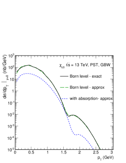
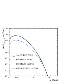
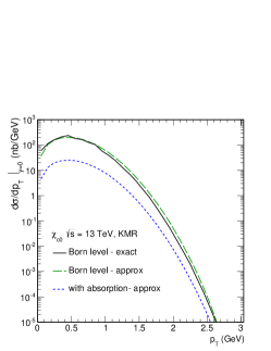
Figure 10: Transverse momentum distribution of $\chi_{c0}$ CEP at $y=0$, with the PST-GBW, the CDHI and Durham prescription.

Table 4: An example of $V_{1}$ values at midrapidity of $\eta_{c}$ in the CEP process, for several prescriptions for off-diagonal UGDs.

$\eta_{c}$	$V_{1}^{-}$ [$\sqrt{\rm nb}/{\rm GeV}^{4}$]	$B_{D}[{\rm GeV}^{-2}]$	$g_{\rm abs}$	$\beta$	$\sigma_{\rm tot}|_{y=0}$ [nb]	$\sigma_{\rm tot}^{\rm abs}|_{y=0}$ [nb]	$S^{2}_{y=0}$
PST GBW	194.	3.4	0.83	0.12	$1.8\times 10^{-2}$	$3.9\times 10^{-3}$	0.21
PST RS	400.	3.2	0.84	0.12	$9.0\times 10^{-3}$	$1.9\times 10^{-3}$	0.21
CDHI GJR08NLO	651.	3.5	0.81	0.13	$1.8\times 10^{-1}$	$4.0\times 10^{-2}$	0.22
KMR GJR08NLO	1015.	4.7	0.76	0.16	$1.3\times 10^{-1}$	$3.0\times 10^{-2}$	0.29
BPSS GJR08NLO	1490.	7.0	0.66	0.20	$5.8\times 10^{-2}$	$2.2\times 10^{-2}$	0.38

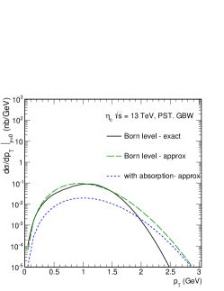
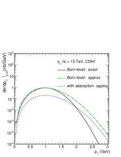
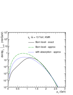
Figure 11: Distribution in transverse momentum of $\eta_{c}$ in the CEP process for PST-GBW, CDHI and Durham prescriptions at $y=0$.

Our amplitude is normalized in such a way that the expression

$$d\sigma={1\over 256\pi^{5}s^{2}}|{\cal M}(Y,y,\mbox{\boldmath$p$}_{1},\mbox{\boldmath$p$}_{2})|^{2}dyd^{2}\mbox{\boldmath$p$}_{1}d^{2}\mbox{\boldmath$p$}_{2}d^{2}\mbox{\boldmath$p$}\,\delta^{(2)}(\mbox{\boldmath$p$}+\mbox{\boldmath$p$}_{1}+\mbox{\boldmath$p$}_{2})$$ (34)

holds. We will now concentrate on central diffractive production, i.e. we fix the meson rapidity to be $y=0$. Below we adopt $\sqrt{s}=13\,{\rm TeV}$. We can therefore forget about the Regge-propagators in Eq. (31), and without loss of generality we write

$$\Phi_{1,2}(\mbox{\boldmath$p$}_{1,2})=\exp\Big{(}-{1\over 2}B_{D}\mbox{\boldmath$p$}^{2}_{1,2}\Big{)}\,.$$ (35)

Then, using the vertices of Eq. (33), the transverse momentum distributions of the mesons at the Born level are obtained as

$${d\sigma^{0+}_{\rm Born}\over dydp^{2}_{T}}\Big{|}_{y=0} = {\exp[-{1\over 2}B_{D}p_{T}^{2}]V_{0}^{2}\over 512\pi^{3}B_{D}}\Big{\{}1-\tau(1-{1\over 2}B_{D}p_{T}^{2})+{\tau^{2}\over 2}\Big{(}1-{1\over 2}B_{D}p_{T}^{2}+{1\over 8}B_{D}^{2}p_{T}^{4}\Big{)}\Big{\}}$$

$${d\sigma^{0-}_{\rm Born}\over dydp_{T}^{2}}\Big{|}_{y=0} = {(V_{1}^{-})^{2}\over 512\pi^{3}}{p_{T}^{2}\over 4B_{D}^{2}}\exp[-{1\over 2}B_{D}p_{T}^{2}]\,.$$ (36)

Now, the absorptive corrections require the evaluation of the loop integral

$$\delta{\cal M}(Y,0,\mbox{\boldmath$p$}_{1},\mbox{\boldmath$p$}_{2}) = \int{d^{2}\mbox{\boldmath$k$}\over 2(2\pi)^{2}}\,T(s,\mbox{\boldmath$k$})\exp\Big{(}-{1\over 2}B_{D}(\mbox{\boldmath$p$}_{1}+\mbox{\boldmath$k$})^{2}\Big{)}\exp\Big{(}-{1\over 2}B_{D}(\mbox{\boldmath$p$}_{2}-\mbox{\boldmath$k$})^{2}\Big{)}$$ (37)

$$\times V(\mbox{\boldmath$p$}_{1}+\mbox{\boldmath$k$},\mbox{\boldmath$p$}_{2}-\mbox{\boldmath$k$})=\exp\Big{(}-{1\over 2}B_{D}(\mbox{\boldmath$p$}_{1}^{2}+\mbox{\boldmath$p$}_{2}^{2})\Big{)}$$

$$\times \int{d^{2}\mbox{\boldmath$k$}\over 2(2\pi)^{2}}\exp\Big{(}-{1\over 2}(B_{\rm el}(s)+2B_{D})\mbox{\boldmath$k$}^{2}-B_{D}\mbox{\boldmath$k$}\cdot(\mbox{\boldmath$p$}_{1}-\mbox{\boldmath$p$}_{2})\Big{)}\,$$

$$\times {\sigma^{pp}_{\rm tot}(s)\,V(\mbox{\boldmath$p$}_{1}+\mbox{\boldmath$k$},\mbox{\boldmath$p$}_{2}-\mbox{\boldmath$k$})}\,.$$

It is useful to introduce the dimensionless quantities

$$g_{\rm abs}={\sigma^{pp}_{\rm tot}(s)\over 4\pi(B_{\rm el}(s)+2B_{D})}\,\quad{\rm and}\quad\,\beta={B_{D}\over B_{\rm el}(s)+2B_{D}}\,.$$ (38)

Then, the absorptive corrections are obtained as

$$\delta{\cal M}^{0+}(Y,0,\mbox{\boldmath$p$}_{1},\mbox{\boldmath$p$}_{2}) = g_{\rm abs}V_{0}\exp\Big{(}-{1\over 2}B_{D}(\mbox{\boldmath$p$}_{1}^{2}+\mbox{\boldmath$p$}_{2}^{2})\Big{)}\,\exp\Big{(}{1\over 2}\beta B_{D}(\mbox{\boldmath$p$}_{1}-\mbox{\boldmath$p$}_{2})^{2}\Big{)}$$

$$\times \Big{\{}1+\beta(1+\beta)\tau B_{D}(\mbox{\boldmath$p$}_{1}^{2}+\mbox{\boldmath$p$}_{2}^{2})+(\mbox{\boldmath$p$}_{1}\cdot\mbox{\boldmath$p$}_{2})\tau B_{D}\Big{(}1-2\beta(1+\beta)\Big{)}\Big{\}}\,,$$

$$\delta{\cal M}^{0-}(Y,0,\mbox{\boldmath$p$}_{1},\mbox{\boldmath$p$}_{2}) = (1-\beta)g_{\rm abs}V_{1}^{-}\exp\Big{(}-{1\over 2}B_{D}(\mbox{\boldmath$p$}_{1}^{2}+\mbox{\boldmath$p$}_{2}^{2})\Big{)}\,\exp\Big{(}{1\over 2}\beta B_{D}(\mbox{\boldmath$p$}_{1}-\mbox{\boldmath$p$}_{2})^{2}\Big{)}$$ (40)

$$\times [\mbox{\boldmath$p$}_{1},\mbox{\boldmath$p$}_{2}](1-\beta)\Big{(}1-\beta B_{D}(\mbox{\boldmath$p$}_{1}\cdot\mbox{\boldmath$p$}_{2})\Big{)}\,,$$

for the scalar and pseudoscalar meson, respectively. We now adjust the constants $V_{0},V_{1}^{\pm}$, as well as $B_{D}$, to our numerical results obtained for the Born-level amplitude.

In Tables 3 and 4, we show the parameters obtained for different prescriptions for the generalized unintegrated gluon distribution, GBW as well as the CDHI and Durham prescriptions for the GJR08NLO gluon distribution. We also show the gap survival factors

$$S^{2}\equiv{d\sigma/dy\Big{|}_{y=0}\over d\sigma_{\rm Born}/dy\Big{|}_{y=0}}\,.$$ (41)

We observe that depending on the gluon distribution used, we obtain for the $\chi_{c}$ the gap survival values of $S^{2}=0.13\div 0.21$, while for the $\eta_{c}$ production they are systematically somewhat higher, $S^{2}=0.21\div 0.38$. Notice, that the $\eta_{c}$ amplitude, due to the vanishing in forward direction, is more peripheral than the one for $\chi_{c}$ production. However also notice that the both reactions have significantly different values of the effective diffraction slopes $B_{D}$. Regarding the diffraction slope we furthermore observe a strong model dependence, especially for the $\eta_{c}$ case.

Our simplified double-Regge approach works reasonably well. In Fig. 10, we show the cross section $d\sigma/dydp_{T}$ at $y=0$ for the $\chi_{c}$ for the three different generalized UGD prescriptions. Shown is the exact numerical result of the Born amplitude (solid line) as well as the result of our effective Regge amplitude fit (long-dashed line). By the short-dashed line we show the differential cross section including absorptive corrections on top of the Regge amplitude Born term. We see from these figures that the effective Regge amplitude form is reasonably accurate for $p_{T}\mathrel{\hbox to0.0pt{\lower 4.0pt\hbox{\hskip 1.0pt$\sim$}\hss}\raise 1.0pt\hbox{$<$}}1.5\,{\rm GeV}$, with a slight ambiguity in the slope $B_{D}$. In the case of the $\eta_{c}$ shown in Fig. 11, the effective Regge fit works almost perfectly for the PST-GBW and CDHI prescriptions, while for the Durham case the description is rather poor.

In our calculation of absorptive corrections, we restricted ourselves to the so-called elastic rescattering correction. We wish to point out, that the often applied multichannel models that account for the possible diffractively excitated intermediate states, are constructed for soft diffractive processes. In our case we deal with a Born level processes with (semi-)hard gluon exchanges, which will favour a coupling to small color dipoles in each proton. It is not clear that the diffractive final states that dominate soft diffractive dissociation at the LHC have a large overlap with the relevant dipole sizes.

In this regard we wish to point to the work of Refs. Pasechnik:2011nw ; Pasechnik:2012ac ; Kopeliovich:2018lha . In these works it is argued, that for certain hard inclusive diffractive processes (part of) the rescattering corrections are in fact already included effectively in the dipole cross section. The consistent formalism for exclusive channels remains an important task for the future.

VII Conclusion

In the present paper we have calculated the key observables of central exclusive $\chi_{c0}$ and $\eta_{c}$ quarkonia production in proton-proton collisions at the LHC within a formalism proposed earlier by the Durham group for central exclusive Higgs boson production.

The $\chi_{c0}$ meson CEP was already computed in the literature previously, while $\eta_{c}$ production has been analysed here for the first time. Compared to the previous calculations we have used here modern versions of collinear gluon distributions to generate off-diagonal unintegrated gluon distributions.

In the present analysis we have also used the $gg\to\eta_{c}$ and $gg\to\chi_{c0}$ transition amplitudes calculated using the light-cone $c\bar{c}$ wave functions obtained in the framework of potential models. We have performed similar calculations for inclusive production of $\eta_{c}$ and $\chi_{c0}$ very recently and showed that one can very well describe the experimental data for $\eta_{c}(1S)$ meson measured in last few years by the LHCb collaboration. Our previous results showed that in the inclusive case the cross section for $\eta_{c}$ is significantly larger than that for $\chi_{c0}$.

It was the main aim of the present paper to make a similar analysis for the exclusive production case, which for the case of $\eta_{c}$ not done so far in the literature. In contrast to the inclusive case, we have found that for the CEP the situation reverses i.e. the corresponding cross section for exclusive $\eta_{c}$ production is considerably smaller than its counterpart for exclusive $\chi_{c0}$ production, at least, for the hard part obtained using the Durham or Cudell et al prescriptions for calculation of the scale in the off-diagonal unintegrated gluon distribution. The reason is a specific interplay of the off-diagonal UGDs and virtual gluon – virtual gluon – quarkonium vertex.

We also proposed a way to calculate the soft effects (in the region of small gluon transverse momenta) using the GBW or RS UGDs, which were obtained from the respective color dipole cross sections, and a simple (PST) prescription for its off-diagonal extrapolation. In this case, the cross section is only slightly smaller for $\eta_{c}$ than for $\chi_{c0}$ production. We have also discussed to which extent the absorption effects for $pp\to pp\eta_{c}$ are different than those for $pp\to pp\chi_{c0}$. We find that the absorptive corrections for the $\eta_{c}$ somewhat smaller, which correlates with a very different $(t_{1},t_{2})$ dependence for the corresponding Born amplitudes. However, there is a rather strong model dependence on the Born-amplitude.

It would be desirable to measure the cross section for $pp\to pp\eta_{c}$ by identifying $\eta_{c}$ e.g. in the $p\bar{p}$ decay channel as was done in the inclusive case. It could be interesting to estimate the signal-to-background ratio before the real experiment. The $pp\to ppp\bar{p}$ continuum was calculated previously by Lebiedowicz, Nachtmann and Szczurek LNS_ppbar and a first experimental evidence was obtained very recently by the STAR collaboration at RHIC STAR_exclusive . Also the $pp\to pp\gamma\gamma$ reaction could be considered as an alternative to measure the $pp\to pp\eta_{c}$ reaction.

References

• (1) V. A. Khoze, A. D. Martin, M. G. Ryskin and W. J. Stirling, Eur. Phys. J. C 35, 211-220 (2004);
L. A. Harland-Lang, V. A. Khoze, M. G. Ryskin and W. J. Stirling, Int. J. Mod. Phys. A 29, 1430031 (2014).
• (2) M. G. Albrow, T. D. Coughlin and J. R. Forshaw, Prog. Part. Nucl. Phys.  65 149 (2010).
• (3) R. S. Pasechnik, A. Szczurek and O. V. Teryaev, Phys. Rev. D 78, 014007 (2008).
• (4) R. S. Pasechnik, A. Szczurek and O. V. Teryaev, Phys. Lett. B 680, 62 (2009).
• (5) R. S. Pasechnik, A. Szczurek and O. V. Teryaev, Phys. Rev. D 81, 034024, (2010).
• (6) P. Lebiedowicz, O. Nachtmann and A. Szczurek, Annals Phys. 344, 301-339 (2014).
• (7) F. Kopp, M. B. Gay Ducati and M. V. T. Machado, Phys. Lett. B 806, 135492 (2020).
• (8) I. Babiarz, R. Pasechnik, W. Schäfer and A. Szczurek, JHEP 02, 037 (2020).
• (9) I. Babiarz, R. Pasechnik, W. Schäfer and A. Szczurek, JHEP 06, 101 (2020).
• (10) R. Aaij et al. [LHCb collaboration], Eur. Phys. J. C 75, no.7, 311 (2015);
R. Aaij et al. [LHCb collaboration], Eur. Phys. J. C 80, no.3, 191 (2020).
• (11) Tichouk, H. Sun and X. Luo, Phys. Rev. D 101, no.9, 094006 (2020).
• (12) I. Babiarz, V. P. Goncalves, R. Pasechnik, W. Schäfer and A. Szczurek, Phys. Rev. D 100, no.5, 054018 (2019).
• (13) A. Szczurek, R. Pasechnik and O. Teryaev, Phys. Rev. D 75, 054021 (2007).
• (14) A. Donnachie and P. V. Landshoff, Phys. Lett. B 185, 403 (1987).
• (15) A. Shuvaev, K. J. Golec-Biernat, A. D. Martin and M. Ryskin, Phys. Rev. D 60, 014015 (1999).
• (16) J. R. Cudell, A. Dechambre, O. F. Hernandez and I. P. Ivanov, Eur. Phys. J. C 61, 369 (2009).
• (17) K. J. Golec-Biernat and M. Wüsthoff, Phys. Rev. D 60, 114023 (1999).
• (18) K. Golec-Biernat and S. Sapeta, JHEP 03, 102 (2018).
• (19) A. H. Rezaeian and I. Schmidt, Phys. Rev. D 88, 074016 (2013) [arXiv:1307.0825 [hep-ph]].
• (20) E. Iancu, K. Itakura and S. Munier, Phys. Lett. B 590, 199-208 (2004) [arXiv:hep-ph/0310338 [hep-ph]].
• (21) P. Jimenez-Delgado and E. Reya, Phys. Rev. D 89 no.7, 074049 (2014).
• (22) M. Gluck, P. Jimenez-Delgado, E. Reya and C. Schuck, Phys. Lett. B 664, 133-138 (2008).
• (23) M. Gluck, E. Reya and A. Vogt, Z. Phys. C 67, 433-448 (1995).
• (24) J. D. Bjorken, Phys. Rev. D 47, 101-113 (1993).
• (25) E. Gotsman, E. Levin and U. Maor, Phys. Rev. D 60, 094011 (1999).
• (26) A. B. Kaidalov, V. A. Khoze, A. D. Martin and M. G. Ryskin, Eur. Phys. J. C 21, 521-529 (2001).
• (27) S. Ostapchenko and M. Bleicher, Eur. Phys. J. C 78, no.1, 67 (2018).
• (28) C. Flensburg, G. Gustafson and L. Lönnblad, JHEP 1212, 115 (2012).
• (29) C. O. Rasmussen and T. Sjöstrand, JHEP 1602, 142 (2016).
• (30) R. S. Pasechnik and B. Z. Kopeliovich, Eur. Phys. J. C 71, 1827 (2011).
• (31) R. Pasechnik, B. Kopeliovich and I. Potashnikova, Phys. Rev. D 86, 114039 (2012).
• (32) B. Z. Kopeliovich, R. Pasechnik and I. K. Potashnikova, Phys. Rev. D 98, no. 11, 114021 (2018).
• (33) L. Lönnblad and R. Žlebčík, Eur. Phys. J. C 76 (2016) no.12, 668.
• (34) I. Babiarz, R. Staszewski and A. Szczurek, Phys. Lett. B 771, 532-538 (2017).
• (35) G. Antchev et al. [TOTEM Collaboration], Eur. Phys. J. C 79, no.2, 103 (2019).
• (36) P. Lebiedowicz, O. Nachtmann and A. Szczurek, Phys. Rev. D97, 094027 (2018).
• (37) J. Adam et al. [STAR Collaboration], JHEP 07, 178 (2020).