Sensitivity of direct detection experiments to neutrino magnetic dipole moments

Abstract

With large active volume sizes dark matter direct detection experiments are sensitive to solar neutrino fluxes. Nuclear recoil signals are induced by ⁸B neutrinos, while electron recoils are mainly generated by the pp flux. Measurements of both processes offer an opportunity to test neutrino properties at low thresholds with fairly low backgrounds. In this paper we study the sensitivity of these experiments to neutrino magnetic dipole moments assuming 1, 10 and 40 tonne active volumes (representative of XENON1T, XENONnT and DARWIN), 0.3 keV and 1 keV thresholds. We show that with nuclear recoil measurements alone a 40 tonne detector could be as competitive as Borexino, TEXONO and GEMMA, with sensitivities of order $8.0\times 10^{-11}\,\mu_{B}$ at the $90\%$ CL after one year of data taking. Electron recoil measurements will increase sensitivities way below these values allowing to test regions not excluded by astrophysical arguments. Using electron recoil data and depending on performance, the same detector will be able to explore values down to $4.0\times 10^{-12}\mu_{B}$ at the $90\%$ CL in one year of data taking. By assuming a 200-tonne liquid xenon detector operating during 10 years, we conclude that sensitivities in this type of detectors will be of order $10^{-12}\,\mu_{B}$. Reducing statistical uncertainties may enable improving sensitivities below these values.

I Introduction

Dark matter (DM) direct detection experiments are already sensitive to solar neutrinos. In its latest data sets, XENON1T has reported signals in both coherent elastic neutrino-nucleus scattering (CE$\nu$NS) and neutrino-electron elastic scattering Aprile et al. (2019, 2020a). It is natural to expect that with increasing active volumes and exposures, XENONnT Aprile et al. (2016), LZ Akerib et al. (2018), and DARWIN Aalbers et al. (2016) will provide larger statistics in both channels. Threfore, their results will enable precise measurements of neutrino properties complementing those coming from present and near-future dedicated neutrino experiments (see, e.g. Deniz et al. (2010); An et al. (2016); Acciarri et al. (2015); Strauss et al. (2017); Hakenmüller et al. (2019); Aguilar-Arevalo et al. (2019)). The opportunities these data offer include—but are not limited to— studies of new interactions in the neutrino sector by means of light vector and scalar mediators, neutrino non-standard interactions, and neutrino electromagnetic properties Baudis et al. (2014); Cerdeño et al. (2016); Dutta et al. (2017); Aristizabal Sierra et al. (2018); Gonzalez-Garcia et al. (2018); Aristizabal Sierra et al. (2019a); Papoulias et al. (2018); Hsieh et al. (2019). They will also provide a playground for precise measurements of solar neutrino fluxes, including those from the solar CNO cycle Newstead et al. (2018), as well as for tests of solar models and solar neutrino matter effects Aalbers et al. (2020).

With precise discrimination, measurements of electron or nuclear recoils alone can determine the presence of new physics. That could be the case—for instance—of the recent electron excess reported by the XENON1T collaboration Aprile et al. (2020a), if indeed new physics is responsible for such a signal. Ideally, a physical explanation of an electron excess would produce a particular signature in the corresponding nuclear channel. However, an observation of a signal e.g. in electron recoils does not necessarily implies an observation of nuclear recoils. The main reason being the energy thresholds involved. For $\sim 0.1\,$keV thresholds, electron recoils are driven by pp neutrino fluxes, while nuclear recoils by ⁸B neutrinos. In $\text{cm}^{-2}\text{s}^{-1}$ units, these fluxes differ by about four orders of magnitude Bahcall et al. (2005). Thus, unless the new physics effects are way more pronounced in the $\nu-N$ cross section, one expects the electron recoil signal to be more prominent (possibly only observable in that channel). An extreme case of such scenario would be a nucleon-phobic light vector mediator, in which case only an excess in electron recoils could be observed.

However, there are other cases in which either the electron or nuclear recoil signal can come along with a signal in the other channel. Arguably the most remarkable example in this case is given by photon exchange. As soon as the new physics couples to photons, depending on the size of the new physics couplings, there will be new contributions to electron and nuclear recoil signals . In the case of neutrino detection, any of its electromagnetic couplings will lead to both electron and nuclear recoils, again depending on their size both processes could be observed. This discussion is of course not only related to neutrinos, a typical example involving DM is given by dark photon portals in which kinetic mixing allows coupling of the dark and visible (SM) sectors Okun (1982); Holdom (1986).

Motivated by the latest XENON1T result Aprile et al. (2020a), in this paper we study the extent at which neutrino electromagnetic properties can be tested at XENON1T, XENONnT and DARWIN using combined electron and nuclear recoil measurements. We consider neutrino magnetic dipole moments and determine the discovery reach under simplified detector and signal assumptions. This includes one, ten and forty tonne active volumes, $100\%$ detector efficiency and $0.3\,\text{keV}$ and $1\,\text{keV}$ energy thresholds. The former motivated by Ref. Lenardo et al. (2019), while the latter determined by future detector performances Aprile et al. (2016); Akerib et al. (2018); Aalbers et al. (2016). In all cases our toy experiments correspond to the SM electron and nuclear recoil spectra (measured in events/tonne/year/keV). For CE$\nu$NS we assume two background hypotheses, $68\%$ and $25\%$ of the signal rate. While for $\nu-e$ elastic scattering we instead use expected backgrounds at XENON1T, XENONnT and DARWIN as given in Refs. Aprile et al. (2020a, b); Aalbers et al. (2020). Needless to say, these assumptions—in particular for CE$\nu$NS—are just representative of how the actual detectors performances and data sets will look like, but allow us to visualize how competitive these detectors will be when compared to neutrino dedicated experiments.

The remainder of this paper is organized as follows. In Sec. II we shortly discuss CE$\nu$NS, $\nu-e$ elastic scattering as well as neutrino magnetic dipole moments and their corresponding differential cross sections. In Sec. III we describe our statistical analysis and present our results. Finally in Sec. IV we summarize and present our conclusions.

II CE$\nu$NS, $\nu-e$ elastic scattering and neutrino magnetic dipole moments

In the SM, CE$\nu$NS is a neutral current process in which the neutrino energy involved, $E_{\nu}\lesssim 100\,$MeV, is such that the transferred momentum implies the individual nucleon amplitudes sum up coherently. This results in an approximately overall enhancement of the cross section, determined by $N^{2}$, where $N$ refers to the number of neutrons of the target nuclei Freedman (1974); Freedman et al. (1977). Given the constraints over the neutrino energy probe, possible neutrinos that can induce the process are limited to neutrinos produced in pion decay-at-rest, reactor and solar neutrinos. Other possible sources include sub-GeV atmospheric neutrinos, diffuse supernova (SN) background (DSNB) neutrinos and a SN burst. However, their detection is less certain. Sub-GeV atmospheric neutrinos and DSNB fluxes are small, and so very large exposures are required for their detection Newstead et al. (2020). Observation of a SN burst is not guaranteed, although it is expected to happen at certain point Lang et al. (2016).

The differential cross section for this process involves a zero-transferred momentum component and a nuclear form factor that accounts for nuclear structure. It is given by Freedman (1974)

$$\frac{d\sigma_{\nu-N}}{dE_{r}}=\frac{G_{F}^{2}}{2\pi}m_{N}g_{N}^{2}\left(2-\frac{m_{N}E_{r}}{E_{\nu}^{2}}\right)\,F^{2}(E_{r})\ .$$ (1)

Here $g_{N}=(A-Z)g_{N}^{n}+Zg_{V}^{p}$, where $g_{N}^{n}=2g_{N}^{d}+g_{N}^{u}$ and $g_{N}^{p}=g_{N}^{d}+2g_{N}^{u}$ with the quark electroweak couplings given by $g_{N}^{d}=-1/2+2/3\sin^{2}\theta_{W}$ and $g_{N}^{u}=1/2-4/3\sin^{2}\theta_{W}$. For the weak mixing angle we use $\sin^{2}\theta_{W}=0.23122$ Patrignani and Group (2016). For the nuclear form factor we adopt the Helm parametrization and assume the the same root-mean-square radii for the proton and neutron distributions. Assuming otherwise requires weighting the neutron and proton contributions with independent form factors Aristizabal Sierra et al. (2019c). Note that for the energies we are interested in the form factor plays a somewhat minor role.

Solar neutrinos are subject to neutrino flavor conversion, which depending on the process of the pp chain they originate from can be matter enhanced. Assuming the two-flavor approximation (mass dominance limit $\Delta m_{13}^{2}\to\infty$), two neutrino flavors reach the detector. One mainly an electron flavor, $\nu_{e}$, with a muon contamination suppressed by the reactor mixing angle. And a second one, $\nu_{a}$, that is a superposition of muon and tau flavors with the admixture controlled by the atmospheric mixing angle. Neutrino-electron scattering induced by solar neutrinos receives therefore contributions from neutral and charged current. Neutral from $\nu_{e}-e$ and $\nu_{a}-e$ interactions, while charged from $\nu_{e}-e$ alone. The differential cross section reads Vogel and Engel (1989)

$$\frac{d\sigma_{\nu-e}}{dE_{r}}=\frac{G_{F}^{2}m_{e}}{2\pi} \left[(g_{V}+g_{A})^{2}+(g_{V}-g_{A})^{2}\left(1-\frac{E_{r}}{E_{\nu}}\right)^{2}\right.$$

$$\left.(g_{A}^{2}-g_{V}^{2})\frac{m_{e}E_{r}}{E_{\nu}^{2}}\right]\ ,$$ (2)

with the vector and axial couplings given by

$$g_{V}=2\sin^{2}\theta_{W}\pm\frac{1}{2}\ ,\qquad g_{A}=\pm\frac{1}{2}\ .$$ (3)

Here ‘$+$’ holds for $\nu_{e}$, while ‘$-$’ for $\nu_{a}$.

II.1 Neutrino magnetic/electric dipole moments and cross sections

Possible neutrino electromagnetic couplings are determined by the neutrino electromagnetic current, which decomposed in terms of electromagnetic form factors leads to four diagonal independent couplings in the zero-transferred momentum limit: electric charge, magnetic dipole moment Fujikawa and Shrock (1980); Schechter and Valle (1981); Pal and Wolfenstein (1982); Kayser (1982); Nieves (1982); Shrock (1982), electric dipole moment and anapole moment Kayser (1982). Depending on whether neutrinos are Dirac or Majorana and on whether CP and CPT are exact symmetries in the new physics sector, some of these couplings may vanish Kayser (1982); Nieves (1982). They are subject to a variety of limits from laboratory experiments Canas et al. (2016) that include PVLAS Della Valle et al. (2016), neutron $\beta$ decay Foot et al. (1990), TRISTAN, LEP and CHARM-II Hirsch et al. (2003), MUNU Daraktchieva et al. (2005), Super-Kamiokande Liu et al. (2004), TEXONO Deniz et al. (2010), GEMMA Beda et al. (2010) and Borexino Phase-II Agostini et al. (2017). They are constrained by cosmology and astrophysical observations as well, including primordial nucleosynthesis Grifols and Masso (1987), neutrino star turning Studenikin and Tokarev (2014), supernova and stellar cooling Barbiellini and Cocconi (1987); Grifols and Masso (1989); Raffelt (1990a, b). For an extensive review on this constraints see Ref. Giunti and Studenikin (2015) (see Ref. Brdar et al. (2020) as well for constraints involving order MeV right-handed neutrinos).

At the effective level the magnetic/dipole couplings can be written according to

$$-\mathcal{L}^{D} =\frac{1}{2}\overline{\nu_{L_{i}}}\sigma_{\mu\nu}\left(\mu_{ij}^{D}+\gamma_{5}\epsilon_{ij}^{D}\right)\nu_{R_{j}}\ +\text{H. c.},$$

$$-\mathcal{L}^{M} =\frac{1}{2}\overline{\nu_{L_{i}}^{c}}\sigma_{\mu\nu}\left(\mu_{ij}^{M}+\gamma_{5}\epsilon_{ij}^{M}\right)\nu_{L_{j}}\ +\text{H. c.}$$ (4)

Note that electron recoil experiments cannot differentiate between Dirac or Majorana couplings, nor between magnetic/electric moments or transitions. In the mass eigenstate basis, processes induced by interactions (II.1) are sensitive to the effective parameter Beacom and Vogel (1999)

$$\mu_{\nu_{\text{eff}}}^{2}=\sum_{j}\left|\sum_{k}A_{k}(E_{\nu},L)(\mu_{kj}-i\epsilon_{kj})\right|^{2}\ ,$$ (5)

where $A_{k}(E_{\nu},L)$ refers to the amplitude of the $k$-th massive neutrino state at detection point. The effective coupling takes different forms depending on whether neutrinos are Dirac or Majorana as well as on the flavor scheme adopted (see e.g. Ref. Canas et al. (2016)). We will therefore use this effective coupling in our calculations, since it can be useful from the phenomenological point of view. As a simple illustration of this point, we can consider the case of diagonal couplings $\mu_{e}$ and $\mu_{a}$. In the two-flavor approximation and for oscillation parameters as required by the LMA-MSW solution the effective coupling takes the form Agostini et al. (2017)

$$\mu_{\nu_{\text{eff}}}^{2}\simeq P_{ee}\mu_{e}^{2}+(1-P_{ee})\mu_{a}^{2}\ .$$ (6)

Here $P_{ee}$ is the electron neutrino survival probability (see discussion in next section) and we have used $\sin^{4}\theta_{13}\ll 1$. The analysis of neutrino magnetic interactions is therefore a multiparameter problem that can be reduced to a single parameter problem with the aid of (5). Using this parametrization, the $\nu-e$ differential cross section reads Vogel and Engel (1989)

$$\frac{d\sigma_{\nu}}{dE_{r}}=\pi\alpha\,\frac{\mu_{\nu_{\text{eff}}}^{2}}{m_{e}^{2}}\left(\frac{E_{\nu}-E_{r}}{E_{r}}\right)\ ,$$ (7)

where $\mu_{\nu_{\text{eff}}}$ has been normalized to the Bohr magneton. For CE$\nu$NS the differential cross section has the same structure but comes along with the number of target protons squared $Z^{2}$ and a nuclear form factor. Because of the Coulomb divergence the cross section is forward peaked, a behavior that becomes rather pronounced at low recoil energies. The most salient feature of neutrino magnetic moment interactions is thus spectral distortions.

Component	Kinematic limit [keV]
pp	$2.64\times 10^{2}$
7Be ($E_{\nu}=0.3\,$MeV)	$2.31\times 10^{2}$
7Be ($E_{\nu}=0.8\,$MeV)	$6.64\times 10^{2}$
pep	$1.18\times 10^{3}$
hep	$1.85\times 10^{4}$
8B	$1.63\times 10^{4}$ $(4.48)$
13N	$9.88\times 10^{2}$
15O	$1.51\times 10^{3}$
17F	$1.52\times 10^{3}$

Table 1: Kinematic recoil energy limit for the different neutrino components of the solar pp and CNO cycles in neutrino-electron scattering. Included as well in parenthesis is the kinematic limit for ⁸B in CE$\nu$NS. The values displayed follow from the BS05 standard solar model Bahcall et al. (2005).

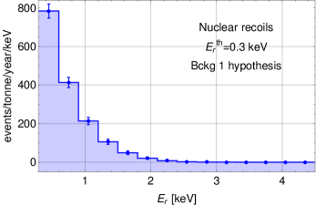
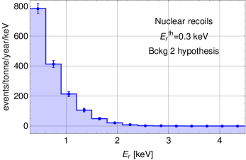
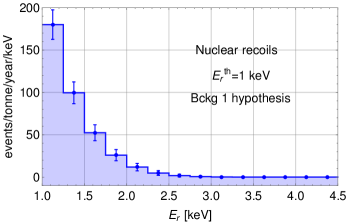
Figure 1: Top graphs: CE$\nu$NS toy experiment signals for a $0.3\,$keV threshold with a background amounting to $68\%$ (left) and $25\%$ (right) of the signal rate, Bckg 1 and Bckg 2 hypotheses respectively. The result assumes 100% detector efficiency and one tonne-year exposure. Bottom graphs: Same as the top graphs but for $1\,$keV threshold instead. For the CE$\nu$NS analysis, these are the “experimental” signals we have assumed. As can be seen, results are rather sensitive to threshold choices.

For all the cross sections we have discussed maximum recoil energies are written as

$$\text{Neutrino-electron}:\quad E_{r}^{\text{max}} =\frac{2E_{\nu}^{2}}{m_{e}+2E_{\nu}}\ ,$$

$$\text{Neutrino-nucleus}:\quad E_{r}^{\text{max}} =\frac{2E_{\nu}^{2}}{m_{N}+2E_{\nu}}\simeq\frac{2E_{\nu}^{2}}{m_{N}}\ ,$$ (8)

with the approximation being fairly good for all isotopes of interest, particularly for xenon.

II.2 Recoil spectra

The recoil spectrum for nuclear and electron recoils proceeds from a convolution of neutrino fluxes and neutrino cross sections. In the case of nuclear recoils, they will be sensitive to all neutrino flavors on equal footing. For electron recoils the situation is different since electron neutrinos are subject as well to charged current processes, while the other flavors do not. Fluxes, therefore, should be weighted by the neutrino oscillation survival probability $P_{ee}$, which proceeds from an average over neutrino trajectory, including all neutrino fluxes $d\Phi/dE_{\nu}$ (pp and CNO cycles) and involving neutrino production distributions as predicted by the standard solar model (see e.g. Aristizabal Sierra et al. (2018)). For its calculation we have employed those given by the BS05 model Bahcall et al. (2005) and the neutrino oscillation parameters best-fit-point values in de Salas et al. (2018). Inclusion of neutrino magnetic moments can involve neutrino oscillation probabilities too, depending on whether the new couplings are or not flavor dependent.

For thresholds above $\sim 0.1\,$keV CE$\nu$NS is sensitive only to the ⁸B neutrino flux (the hep flux is too suppressed to give a sizable signal). Neutrino-electron elastic scattering instead is sensitive to all solar neutrino fluxes, and so it is dominated by pp neutrinos. Contribution form other fluxes is small, with the main contribution given by the $0.86\,$MeV ⁷Be line (see e.g. Aristizabal Sierra et al. (2020)). We write then the recoil spectra as follows

$$\frac{dR_{\nu-N}}{dE_{r}}= N_{N}\int_{E_{\text{min}}}^{E_{\text{max}}}\,\frac{d\Phi_{{}^{8}\text{B}}}{dE_{\nu}}\left[\frac{d\sigma_{\nu-N}}{dE_{r}}+\frac{d\sigma_{\nu}}{dE_{r}}\right]dE_{\nu}\ ,$$

$$\frac{dR_{\nu-e}}{dE_{r}}= N_{e}\int_{E_{\text{min}}}^{E_{\text{max}}}\,\sum_{\alpha}\frac{d\Phi_{\alpha}}{dE_{\nu}}\left[P_{ee}\frac{d\sigma_{\nu-e}}{dE_{r}}\right.$$

$$\left.+(1-P_{ee})\frac{d\sigma_{\nu_{a}}}{dE_{r}}+\frac{d\sigma_{\nu}}{dE_{r}}\right]dE_{\nu}\ .$$ (9)

Here $N_{N}$ and $N_{e}$ refer to the number of nuclei and electrons in the detector, $E_{\nu}^{\text{min}}=\sqrt{m_{N}E_{r}/2}$ for CE$\nu$NS and $E_{\nu}^{\text{min}}=[E_{r}+(E_{r}^{2}+2E_{r}m_{e})^{1/2}]/2$ for $\nu-e$ scattering. Index $\alpha$ runs over pp, ⁸B, hep, ⁷Be, pep ¹³N, ¹⁵O and ¹⁷F. $E_{\nu}^{\text{max}}$ is determined by the kinematic tail of the corresponding flux as displayed in Tab. 1.

III Sensitivity to neutrino magnetic moments

Xenon multi-ton scale DM detectors rely on photon (scintillation) and electron (ionization) signals Aprile et al. (2016); Aalbers et al. (2016). Photons are detected through photosensors that produce a prompt S1 signal. Electrons, instead, are drifted upwards with the aid of an electric field, resulting in a delayed S2 signal. S1 and S2 signals in turn allow the reconstruction of the radial position and depth of a given interaction, together with the energy reconstruction of an event. Their ratio, S2/S1, provides a way to descriminate between electron and nuclear recoils. Moreover, the dual-phase technology, allows to get more information on the S2 signal improving the resolution power of these detectors. The combination of these features provides a powerful tool for event selection over background and this will eventually enable the reconstruction of new physics signals, if any, through the discrimination of electronic and nuclear signatures.

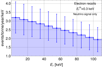
Figure 2: Neutrino-electron signal for a $0.3\,$keV threshold with error bars amounting to $68\%$ of the signal rate. The calculation assumes 100% detector efficiency and a one tonne-year exposure. Results are rather insensitive to threshold shifts (0.3 keV to 1 keV).

To assess the sensitivity of direct detection experiments to neutrino magnetic moments we use a spectral chi-square test assuming various detector configurations as follows. One, ten and forty tonne active volume sizes, 0.3 keV and 1 keV thresholds. For CE$\nu$NS we adopt two background hypotheses, $68\%$ and $25\%$ of the signal rate. For $\nu-e$ elastic scattering instead we use the expected backgrounds at XENON1T, XENONnT and DARWIN reported in Refs. Aprile et al. (2020a, b); Aalbers et al. (2020). They include material radioactivity, double beta decays of ¹³⁶Xe and ¹²⁴Xe decays via double electron capture, among others. Although we take these assumptions as representative of XENON1T, XENONnT and DARWIN, their main motivation is that of comparing the impact of different active volumes as well as different thresholds and backgrounds in the reach of direct detection experiments to neutrino electromagnetic properties.

Under these assumptions we first calculate the signals that define our toy experiments for both CE$\nu$NS and $\nu-e$ elastic scattering, considered in all cases as the SM prediction ($\mu_{\nu_{\text{eff}}}=0$). For CE$\nu$NS, recoil energies are taken up to the ⁸B kinematic threshold, $\sim 4.5\,$keV. For $\nu-e$ scattering the pp-induced signal extends up to 264 keV (see Tab. 1). However, we consider recoil energies only up to $105\,$keV, point at which the signal drops. Covering up to the kinematic limit does not have a substantial impact in our results. The resulting toy experiments signals are shown in Fig. 1 for CE$\nu$NS and in Fig. 2 for $\nu-e$ scattering. Note that we have only shown signals at different thresholds for the case of CE$\nu$NS. We found that for $\nu-e$ scattering, changing the threshold from $0.3\,$keV to $1\,$keV has a negligible effect, which means that toy experiments for any of those thresholds produce, in practice, the same signal. The reason is justified by the fact that the $0.7\,$keV shift in energy threshold for $\nu-e$ scattering in the region of interest, reduces the energy range by 0.7%, while for CE$\nu$NS by 15%.

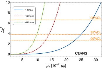
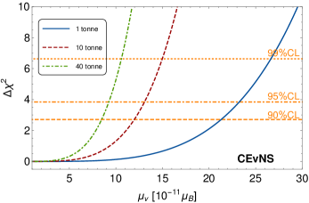
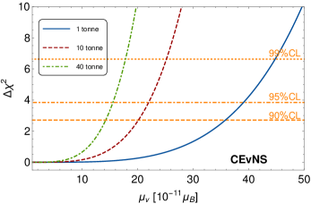
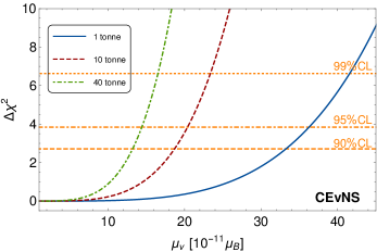
Figure 3: Top graphs: Nuclear recoil sensitivities to neutrino magnetic dipole moments in a 1, 10 and 40 tonne active volume detectors during a one-year data taking. The result assumes a $0.3\,$keV threshold, $100\%$ detector efficiency and backgrounds amounting to $68\%$ (left) and $25\%$ (right) of the signal rate, Bckg 1 and 2 hypotheses respectively. Bottom graphs: Same as top graphs, but assuming a $1\,$keV threshold. In contrast to electron recoils, results are rather sensitive to threshold performances.

We define our binned chi-square test according to

$$\chi^{2}=\sum_{i}\frac{1}{\sigma_{i}^{2}}\left(\left.\frac{dR_{i}}{dE_{r}}\right|_{\text{SM}}-\left.\frac{dR_{i}}{dE_{r}}\right|_{\mu_{\nu_{\text{eff}}}}\right)^{2}\ ,$$ (10)

where the recoil spectra in the second term includes both the SM and neutrino magnetic moment contributions to the signal. For our analysis we sample over $\mu_{\nu_{\text{eff}}}$ from $10^{-9}\,\mu_{B}$ and as low as $10^{-13}\,\mu_{B}$ for both CE$\nu$NS and $\nu-e$ scattering channels. The results of the analysis are shown in Fig. 3, which display $\Delta\chi^{2}$ versus $\mu_{\nu_{\text{eff}}}$ (in $\mu_{B}$ units) calculated for the four different combinations in Fig. 1. The results for different active volume sizes are shown in each plot, proving that an enhancement from 1 to 40 tonne (XENON1T to DARWIN) will improve the sensitivity by a factor $\sim 2.5$ at the $90\%$CL. As can be seen this sensitivity factor enhancement is independent of threshold and background conditions.

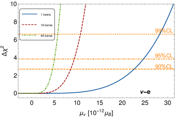
Figure 4: Electron recoil sensitivities to neutrino magnetic dipole moments in 1, 10 and 40 tonne active volume detectors during a one-year data taking. The result assumes a $0.3\,$keV threshold, $100\%$ detector efficiency and backgrounds for XENON1T, XENONnT and DARWIN as given in Refs. Aprile et al. (2020a, b); Aalbers et al. (2020). The result is rather insensitive to threshold shifts (0.1 keV to 1 keV).

A direct comparison of the results can be done as follows: panels in the same row share the same threshold, while those in the same column share the same background hypothesis. We can conclude that decreasing backgrounds may allow a sensitivity enhancement of order $15\%$ at the $90\%$CL. Clearly, our background hypotheses are somewhat arbitrary. Changing them will quantitatively affect this conclusion, but the qualitative feature will be unchanged. Changing the threshold—as expected—has a similar impact on sensitivities, they are degraded by going from 0.3 keV to 1 keV. Overall the best sensitivity is obtained with a 40-tonne active volume with low background and threshold, top-right graph where we can see that values as small as $8.0\times 10^{-11}\mu_{B}$ at the $90\%$CL can be explored. This result is remarkable since it shows that if a $0.3\,$keV threshold is attainable, experiments with characteristics as those of DARWIN will be able to explore regions in parameter space rather comparable to those explored by Borexino, TEXONO and GEMMA Agostini et al. (2017); Deniz et al. (2010); Beda et al. (2010) even in nuclear recoil measurements. Furthermore, it demonstrates that even in its nuclear recoil data sets DARWIN will be able to test regions close to those not yet ruled out by astrophysical arguments, $\mu_{\nu}|_{\text{astro}}\lesssim 3\times 10^{-12}\,\mu_{B}$ Raffelt (1990b). If such threshold is not achievable, and measurements are “limited” to 1 keV threshold instead, with low backgrounds still sensitivities like those of Borexino, TEXONO and GEMMA will be within reach in the nuclear recoil channel as the bottom-right graph in Fig. 3 shows.

For the neutrino-electron scattering case sensitivities are way better, as expected. Results of our analysis for this process are shown in Fig. 4, which displays $\Delta\chi^{2}$ versus $\mu_{\nu_{\text{eff}}}$. They have been obtained by using the toy experiment signal shown in Fig. 2, and by sampling over $\mu_{\nu_{\text{eff}}}$ in the same range as in the CE$\nu$NS analysis. Thanks to the low thresholds and large volume sizes, sensitivities will outpass those achieved in Borexino, TEXONO and GEMMA even in the 1-tonne detector case (representative of XENON1T). At the 90%CL sensitivities reach values of order $2.3\times 10^{-11}\mu_{B}$. Considering the 40-tonne detector instead, sensitivities improve to values of about $4\times 10^{-12}\mu_{B}$ at the 90%CL.

These values are of the same order and can become more competitive than those derived from astrophysical arguments, which then brings the question of the sensitivities that could be reached with other detector configurations. This question is particularly relevant in the light of existing theoretical bounds derived using effective theories or renormalizable models, which lead to values of about $10^{-14}\,\mu_{B}$ Babu and Mohapatra (1990); Barr et al. (1990); Bell et al. (2005); Davidson et al. (2005); Bell et al. (2006). If one takes the bound from astrophysical arguments at face value, the region of interest then spans roughly two orders of magnitude.

To determine the degree at which the full region can be covered we have calculated the sensitivity in electron recoils that could be achieved in a hypothetical 200-tonne liquid xenon detector under the most favorable assumptions in ten years of data taking. We regard this case as the most optimistic one, and so it fixes the most ambitious sensitivity one could expect. The result is displayed in Fig. 5, which shows $\Delta\chi^{2}$ versus $\mu_{\nu_{\text{eff}}}$ for the assumed configurations. The result includes as well an additional background assumption amounting to $5\%$ of the signal rate, background 3 hypothesis. This result shows that if low thresholds are achieved in this type of detectors, the final sensitivity to neutrino magnetic dipole moments will be of order $10^{-12}\,\mu_{B}$ with little dependence on background. Under the background 2 hypothesis the best sensitivity that can be achieved is about $1.9\times 10^{-12}\,\mu_{B}$ at the 90%CL, while with the background 3 hypothesis this value improves to $1.8\times 10^{-13}\,\mu_{B}$ at the 90%CL. Finally, we have checked whether reducing statistical uncertainties could allow further improvements of these sensitivities. Assuming the background 3 hypothesis and reducing $\sigma_{a}$ in Eq. (10) by a $0.1$ factor we have found that sensitivities could improve close to values of order $10^{-13}\,\mu_{B}$.

In summary one can can fairly say that the full region of interest cannot be covered, but perhaps a reasonable fraction of it could. Whether this is the case will largely depend on the size of statistical uncertainties. If they are substantially reduced, these detectors could eventually test regions of parameter space where non-zero neutrino magnetic moments could induce sizable signals.

IV Conclusions

With large fiducial volumes DM direct detection experiments are sensitive to solar neutrinos fluxes. Indeed, the statistics in both nuclear and electron recoils is expected to be large. This is the case, for instance, in XENON1T which has already collected a substantial number of events in both channels Aprile et al. (2019, 2020a). Motivated by the large statistics expected, in this paper we have studied the sensitivity of those measurements to neutrino magnetic dipole moments. We have considered different detector configurations, which although rather generic are representative of XENON1T, XENONnT and DARWIN. By generating toy experiments signals given by the SM prediction plus two background hypotheses for nuclear recoils ($68\%$ and $25\%$ of the signal rate) and actual background for electron recoils, we have done a chi-square test analysis to determine the reach these detectors would have.

In the case of CE$\nu$NS we have found that sensitivities can be comparable to those reached by neutrino-electron elastic scattering dedicated experiments such as TEXONO, Borexino and GEMMA Deniz et al. (2010); Agostini et al. (2017); Beda et al. (2010). The best sensitivity can be achieved with the 40-tonne detector, with a 0.3 keV threshold and low background. In one year of data taking such detector could explore regions in parameter space down to values of order $8.0\times 10^{-11}\mu_{B}$ at the 90%CL. The 1-tonne detector operating with the same threshold and low background as well could achieve values of about $21.5\times 10^{-11}\,\mu_{B}$ at the 90% CL. These sensitivities can be certainly improved with larger data taking times, but even assuming only one year is already sufficient to make nuclear recoil measurements competitive with current limits.

Sensitivities with neutrino-electron elastic scattering are way better. Furthermore, they are rather insensitive to recoil thresholds. Shifting from $0.3$ keV to $1$ keV changes the events/tonne/year rate in less than 1%. In the ideal case of a 40-tonne detector with a 0.3 keV threshold, regions with values as small as $\sim 4.0\times 10^{-12}\mu_{B}$ at the 90%CL could be explored. This means that using electron recoil measurements these detectors can explore regions of parameter space not yet ruled out by astrophysical arguments. We have found that even the 1-tonne detector might be able to reach values of order $2.3\times 10^{-11}\mu_{B}$ at the 90%CL in only one year of data taking. Note that this result is inline with the neutrino magnetic hypothesis considered by XENON1T in its electron excess analysis Aprile et al. (2020a). These results show that searches for neutrino magnetic signals are already dominated by this type of detectors and will keep being so in the future.

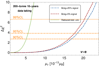
Figure 5: Electron recoil sensitivities to neutrino magnetic dipole moments in a 200-tonne liquid xenon detector under the background 2 and background 3 hypotheses ($25\%$ and $5\%$ of the signal rate) assuming 100% detector efficiency. Results from an analysis with a reduced statistical uncertainty are given by the dotted green curve. The result is obtained for 10 years of data taking.

Finally, we have quantified the degree at which these detectors could cover the $10^{-14}\mu_{B}-10^{-12}\mu_{B}$ region with increasing data taking. To do so we calculated sensitivities for a hypothetical 200-tonne detector under two background hypotheses, $25\%$ and $5\%$ of the signal rate and 10 years of data taking. Our findings show that under these—somewhat extreme—conditions, sensitivities can reach values of order $1.9\times 10^{-12}\,\mu_{B}$ ($1.8\times 10^{-12}\,\mu_{B}$) at the 90%CL for the background 2 (background 3) hypothesis. Covering the full region of interest seems unlikely, but a reasonable fraction is potentially testable if statistical uncertainties can be further suppressed. These detectors thus have a chance to eventually observe neutrino magnetic moment induced signals.

References

- Aprile et al. (2019) E. Aprile et al. (XENON), Phys. Rev. Lett. 123, 251801 (2019), eprint 1907.11485.
- Aprile et al. (2020a) E. Aprile et al. (XENON) (2020a), eprint 2006.09721.
- Aprile et al. (2016) E. Aprile et al. (XENON), JCAP 1604, 027 (2016), eprint 1512.07501.
- Akerib et al. (2018) D. S. Akerib et al. (LUX-ZEPLIN) (2018), eprint 1802.06039.
- Aalbers et al. (2016) J. Aalbers et al. (DARWIN), JCAP 1611, 017 (2016), eprint 1606.07001.
- Deniz et al. (2010) M. Deniz et al. (TEXONO), Phys. Rev. D 81, 072001 (2010), eprint 0911.1597.
- An et al. (2016) F. An et al. (JUNO), J. Phys. G 43, 030401 (2016), eprint 1507.05613.
- Acciarri et al. (2015) R. Acciarri et al. (DUNE) (2015), eprint 1512.06148.
- Strauss et al. (2017) R. Strauss et al., Eur. Phys. J. C77, 506 (2017), eprint 1704.04320.
- Hakenmüller et al. (2019) J. Hakenmüller et al., Eur. Phys. J. C 79, 699 (2019), eprint 1903.09269.
- Aguilar-Arevalo et al. (2019) A. Aguilar-Arevalo et al. (CONNIE) (2019), eprint 1906.02200.
- Baudis et al. (2014) L. Baudis, A. Ferella, A. Kish, A. Manalaysay, T. Marrodan Undagoitia, and M. Schumann, JCAP 01, 044 (2014), eprint 1309.7024.
- Cerdeño et al. (2016) D. G. Cerdeño, M. Fairbairn, T. Jubb, P. A. N. Machado, A. C. Vincent, and C. Boehm, JHEP 05, 118 (2016), [Erratum: JHEP09,048(2016)], eprint 1604.01025.
- Dutta et al. (2017) B. Dutta, S. Liao, L. E. Strigari, and J. W. Walker, Phys. Lett. B773, 242 (2017), eprint 1705.00661.
- Aristizabal Sierra et al. (2018) D. Aristizabal Sierra, N. Rojas, and M. H. G. Tytgat, JHEP 03, 197 (2018), eprint 1712.09667.
- Gonzalez-Garcia et al. (2018) M. C. Gonzalez-Garcia, M. Maltoni, Y. F. Perez-Gonzalez, and R. Zukanovich Funchal, JHEP 07, 019 (2018), eprint 1803.03650.
- Aristizabal Sierra et al. (2019a) D. Aristizabal Sierra, B. Dutta, S. Liao, and L. E. Strigari, JHEP 12, 124 (2019a), eprint 1910.12437.
- Papoulias et al. (2018) D. K. Papoulias, R. Sahu, T. S. Kosmas, V. K. B. Kota, and B. Nayak (2018), eprint 1804.11319.
- Hsieh et al. (2019) C.-C. Hsieh, L. Singh, C.-P. Wu, J.-W. Chen, H.-C. Chi, C.-P. Liu, M. K. Pandey, and H. T. Wong, Phys. Rev. D 100, 073001 (2019), eprint 1903.06085.
- Newstead et al. (2018) J. L. Newstead, L. E. Strigari, and R. F. Lang (2018), eprint 1807.07169.
- Aalbers et al. (2020) J. Aalbers et al. (DARWIN) (2020), eprint 2006.03114.
- Bahcall et al. (2005) J. N. Bahcall, A. M. Serenelli, and S. Basu, Astrophys. J. 621, L85 (2005), eprint astro-ph/0412440.
- Aristizabal Sierra et al. (2019b) D. Aristizabal Sierra, V. De Romeri, and N. Rojas, JHEP 09, 069 (2019b), eprint 1906.01156.
- Okun (1982) L. Okun, Sov. Phys. JETP 56, 502 (1982).
- Holdom (1986) B. Holdom, Phys. Lett. B166, 196 (1986).
- Lenardo et al. (2019) B. Lenardo et al. (2019), eprint 1908.00518.
- Freedman (1974) D. Z. Freedman, Phys. Rev. D9, 1389 (1974).
- Freedman et al. (1977) D. Z. Freedman, D. N. Schramm, and D. L. Tubbs, Ann. Rev. Nucl. Part. Sci. 27, 167 (1977).
- Newstead et al. (2020) J. L. Newstead, R. F. Lang, and L. E. Strigari (2020), eprint 2002.08566.
- Lang et al. (2016) R. F. Lang, C. McCabe, S. Reichard, M. Selvi, and I. Tamborra, Phys. Rev. D94, 103009 (2016), eprint 1606.09243.
- Patrignani and Group (2016) C. Patrignani and P. D. Group, Chinese Physics C 40, 100001 (2016), URL http://stacks.iop.org/1674-1137/40/i=10/a=100001.
- Aristizabal Sierra et al. (2019c) D. Aristizabal Sierra, J. Liao, and D. Marfatia, JHEP 06, 141 (2019c), eprint 1902.07398.
- Vogel and Engel (1989) P. Vogel and J. Engel, Phys. Rev. D39, 3378 (1989).
- Fujikawa and Shrock (1980) K. Fujikawa and R. Shrock, Phys. Rev. Lett. 45, 963 (1980).
- Schechter and Valle (1981) J. Schechter and J. W. F. Valle, Phys. Rev. D24, 1883 (1981), err. D25, 283 (1982).
- Pal and Wolfenstein (1982) P. B. Pal and L. Wolfenstein, Phys. Rev. D25, 766 (1982).
- Kayser (1982) B. Kayser, Phys. Rev. D 26, 1662 (1982).
- Nieves (1982) J. F. Nieves, Phys. Rev. D 26, 3152 (1982).
- Shrock (1982) R. E. Shrock, Nucl. Phys. B206, 359 (1982).
- Canas et al. (2016) B. Canas, O. Miranda, A. Parada, M. Tortola, and J. W. Valle, Phys. Lett. B 753, 191 (2016), [Addendum: Phys.Lett.B 757, 568–568 (2016)], eprint 1510.01684.
- Della Valle et al. (2016) F. Della Valle, A. Ejlli, U. Gastaldi, G. Messineo, E. Milotti, R. Pengo, G. Ruoso, and G. Zavattini, Eur. Phys. J. C 76, 24 (2016), eprint 1510.08052.
- Foot et al. (1990) R. Foot, G. C. Joshi, H. Lew, and R. Volkas, Mod. Phys. Lett. A 5, 95 (1990), [Erratum: Mod.Phys.Lett.A 5, 2085 (1990)].
- Hirsch et al. (2003) M. Hirsch, E. Nardi, and D. Restrepo, Phys. Rev. D 67, 033005 (2003), eprint hep-ph/0210137.
- Daraktchieva et al. (2005) Z. Daraktchieva et al. (MUNU), Phys. Lett. B 615, 153 (2005), eprint hep-ex/0502037.
- Liu et al. (2004) D. Liu et al. (Super-Kamiokande), Phys. Rev. Lett. 93, 021802 (2004), eprint hep-ex/0402015.
- Beda et al. (2010) A. Beda, V. Brudanin, V. Egorov, D. Medvedev, V. Pogosov, M. Shirchenko, and A. Starostin (2010), eprint 1005.2736.
- Agostini et al. (2017) M. Agostini et al. (Borexino), Phys. Rev. D 96, 091103 (2017), eprint 1707.09355.
- Grifols and Masso (1987) J. Grifols and E. Masso, Mod. Phys. Lett. A 2, 205 (1987).
- Studenikin and Tokarev (2014) A. I. Studenikin and I. Tokarev, Nucl. Phys. B 884, 396 (2014), eprint 1209.3245.
- Barbiellini and Cocconi (1987) G. Barbiellini and G. Cocconi, Nature 329, 21 (1987).
- Grifols and Masso (1989) J. Grifols and E. Masso, Phys. Rev. D 40, 3819 (1989).
- Raffelt (1990a) G. G. Raffelt, Phys. Rept. 198, 1 (1990a).
- Raffelt (1990b) G. Raffelt, Phys. Rev. Lett. 64, 2856 (1990b).
- Giunti and Studenikin (2015) C. Giunti and A. Studenikin, Rev. Mod. Phys. 87, 531 (2015), eprint 1403.6344.
- Brdar et al. (2020) V. Brdar, A. Greljo, J. Kopp, and T. Opferkuch (2020), eprint 2007.15563.
- Beacom and Vogel (1999) J. F. Beacom and P. Vogel, Phys. Rev. Lett. 83, 5222 (1999), eprint hep-ph/9907383.
- de Salas et al. (2018) P. F. de Salas, D. V. Forero, C. A. Ternes, M. Tortola, and J. W. F. Valle, Phys. Lett. B782, 633 (2018), eprint 1708.01186.
- Aristizabal Sierra et al. (2020) D. Aristizabal Sierra, V. De Romeri, L. Flores, and D. Papoulias (2020), eprint 2006.12457.
- Aprile et al. (2020b) E. Aprile et al. (XENON) (2020b), eprint 2007.08796.
- Babu and Mohapatra (1990) K. Babu and R. Mohapatra, Phys. Rev. Lett. 64, 1705 (1990).
- Barr et al. (1990) S. M. Barr, E. Freire, and A. Zee, Phys. Rev. Lett. 65, 2626 (1990).
- Bell et al. (2005) N. F. Bell, V. Cirigliano, M. J. Ramsey-Musolf, P. Vogel, and M. B. Wise, Phys. Rev. Lett. 95, 151802 (2005), eprint hep-ph/0504134.
- Davidson et al. (2005) S. Davidson, M. Gorbahn, and A. Santamaria, Phys. Lett. B 626, 151 (2005), eprint hep-ph/0506085.
- Bell et al. (2006) N. F. Bell, M. Gorchtein, M. J. Ramsey-Musolf, P. Vogel, and P. Wang, Phys. Lett. B 642, 377 (2006), eprint hep-ph/0606248.