QBMMlib: A library of quadrature-based moment methods

Abstract

QBMMlib is an open source Mathematica package of quadrature-based moment methods and their algorithms. Such methods are commonly used to solve fully-coupled disperse flow and combustion problems, though formulating and closing the corresponding governing equations can be complex. QBMMlib aims to make analyzing these techniques simple and more accessible. Its routines use symbolic manipulation to formulate the moment transport equations for a population balance equation and a prescribed dynamical system. However, the resulting moment transport equations are unclosed. QBMMlib trades the moments for a set of quadrature points and weights via an inversion algorithm, of which several are available. Quadratures then closes the moment transport equations. Embedded code snippets show how to use QBMMlib, with the algorithm initialization and solution spanning just 13 total lines of code. Examples are shown and analyzed for linear harmonic oscillator and bubble dynamics problems.

Version	v1.0
Link to code	github.com/sbryngelson/QBMMlib
License	GPL 3
Versioning	git
Language	Wolfram Language / Mathematica
Requirements	Mathematica v8.0+
Support email	spencer@caltech.edu

Table 1: Code metadata

1 Motivation and significance

QBMMlib is an open-source library and solves population balance equations (PBEs) using quadrature-based moment methods (QBMMs). PBEs model the evolution of a number density function (NDF) [1, 2, 3, 4, 5]. Such models are useful, for example, in fluid dynamics simulations involving dispersions, wherein the NDF evolution can represent growth, shrinkage, coalescence, breakup, and relative motion [6, 7, 8, 9, 10, 11, 12, 13, 14], Example engineering applications of this are combustion (e.g. soot dynamics in flames) [15, 16, 17, 18] and aerosols (e.g. sprays) [19, 20, 21].

PBEs can be solved by the method of classes [22, 23] or the method of moments (MOM) [24, 25]. QBMMlib employs the MOM because it can more naturally handle problems with multiple internal coordinates (e.g. velocities). Figure 1 shows a typical QBMM-based solution procedure. The MOM represents the NDF via a set of statistical moments and the transport equations for them follow from the PBE. Inverting the moments to a set of weights and abscissas provides a basis for approximating the unclosed transport equations via quadrature (QMOM) [26].

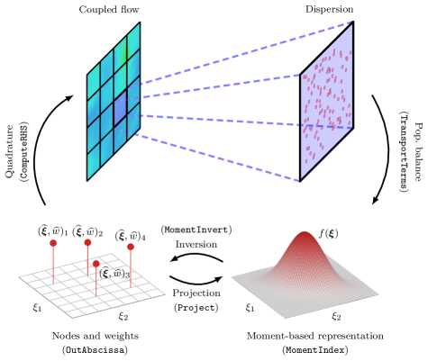
Figure 1: Schematic illustration of the QMOM solution method for flowing dispersions. QBMMlib routines are in parentheses.

Variations on QMOM are plentiful. One can change the inversion procedure: Wheeler’s algorithm can solve single internal coordinate problems [27] and algorithms exist for enforcing distribution shape (extended-QMOM (EQMOM) [28], anisotropic-Gaussian [29, 30]) and hyperbolicity (hyperbolic-QMOM (HyQMOM) [31]). The quadrature weights and abscissas can also evolve directly (direct-QMOM (DQMOM) [32, 33, 34]). One complication is that multiple internal coordinate problems do not admit a unique choice in moment set [35]. However, conditioning one direction on the others provides a particularly robust moment inversion technique (conditional-QMOM (CQMOM) [36] and -HyQMOM (CHyQMOM) [37]). For these reasons, QBMMlib uses Wheeler’s algorithm (or its adaptive counterpart) or HyQMOM for one-dimensional moment inversion and CQMOM and CHyQMOM handle multi-dimensional problems.

There is one other actively developed open source QBMM solver: OpenQBMM [38, 39]. It is a library for OpenFOAM [40] and implements CQMOM and (3-node) CHyQMOM. MFiX [41, 32] and Fluidity [42] use DQMOM, though modern conditional methods (e.g. CQMOM and CHyQMOM) generally outperform it [7]. Note that these are fully-coupled flow solvers. QBMMlib instead decouples these problems and solves the moment transport equations directly for an input dynamical system. This makes it preferable for prototyping and testing on novel physical problems. In pursuit of this, QBMMlib places emphasis on expressive programming, simple interfaces, and symbolic computation where possible. As a result, it can solve PBE-based problems with just a few lines of code.

Section 2 describes QBMMlib’s implementation of the PBE and QBMMs. Section 3 verifies its methods and demonstrates its capabilities for three example problems. Section 4 discusses the utility and novelty of QBMMlib, which concludes the paper.

2 Software description

QBMMlib is a collection of Mathematica functions for solving PBEs via QBMMs. Table 2 describes the public-facing routines. These routines are also documented and accessible in Mathematica via

• Get["QBMMlib"];?QBMMlib`*

Figure 1 illustrates their places in the model and its solution procedure. TransportTerms computes the moment transport equations for the moment set of MomentIndex. MomentInvert inverts these moments to weights and abscissas that close the moment set via quadrature (ComputeRHS) and project it onto a realizable moment space (Project). The next sections describe the details of these routines.

TransportTerms	Input:	Governing equation (eqn, e.g. (1)) and its variables
	Output:	Coefficients (coefs) and exponents (exps) of moment transport equations
MomentIndex	Input:	Number of nodes (n, $N_{\boldsymbol{\widehat{\xi}}}$), inversion method (method)
	Output:	Moment set indices (momidx, $\vec{\bm{k}}$)
	Options:	Number of permutations (default: 1)
MomentInvert	Input:	Moment set (moments, $\vec{\bm{M}}$) and its indices
	Output:	Optimal set of abscissas (xi, $\boldsymbol{\widehat{\xi}}$) and weights (w, $\bm{\widehat{w}}$)
	Options:	Method, Permutation (default: 12 ($\xi_{1}|\xi_{2}$), $N_{\boldsymbol{\xi}}>1$ only)
ComputeRHS	Input:	Abscissas, weights, moment set indices, transport coefficients
	Output:	Right-hand-side of moment transport equation (rhs, $\vec{\bm{F}}$)
	Options:	Third coordinate direction abscissas ($N_{\boldsymbol{\xi}}=2$ only)
Project	Input:	Abscissas, weights, moment set indices
	Output:	Projected moment set (momentsP, $\vec{\bm{M}}$)
OutAbscissa	Input:	Abscissas
	Output:	Threaded abscissas

Table 2: Example public-facing routines. Parenthetical variables correspond to the code snippets and notation of section 2.

2.1 Population balance equations $\mathrm{(}\mathtt{TransportTerms}\mathrm{)}$

QBMMlib can solve one- and two-dimensional populations balance equations. A third direction can be added if its NDF is stationary. The two-dimensional case is detailed here without loss of generality. For illustration, consider

$$\ddot{x}=g(x,\dot{x}),$$ (1)

where the dots indicate partial time derivatives, $g$ is a function, and $\boldsymbol{\xi}=\{x,\dot{x}\}$ are the internal coordinates. The number density function $f$ describes the state and statistics of this system in the $\boldsymbol{\xi}$-space. A population balance equation (PBE) governs $f$ as

$$\frac{\partial f}{\partial t}+\frac{\partial}{\partial x}(f\dot{x})+\frac{\partial}{\partial\dot{x}}(f\ddot{x})=0,$$ (2)

where the zero right-hand-side indicates conservation of $f$, though sinks and sources can model aggregation and breakup [35]. Quadrature-based methods to solving (2) represent $f$ by a set of raw moments $\vec{\bm{M}}$ as $f(\vec{\bm{M}})$. The moment indices $\vec{\bm{k}}=\{l,m\}=\{(0,0),\dots\}$ associated the carried moment set $\vec{\bm{M}}=\{M_{l,m}\}$ depend upon the moment inversion procedure and the number of quadrature points (details follow in section 2.2).

The raw moments are

$$M_{p_{1},\dots,p_{N_{\boldsymbol{\xi}}}}\equiv\int_{\Omega}f(\boldsymbol{\xi})\prod_{j=1}^{N_{\boldsymbol{\xi}}}\xi_{j}^{p_{j}}\text{d}\xi_{j}$$ (3)

where $p_{j}$ (for $j=1,\dots,N_{\boldsymbol{\xi}}$) are the moment indices, $N_{\boldsymbol{\xi}}$ is the number of internal coordinates ($N_{\boldsymbol{\xi}}=2$ in (1)), and $\Omega$ is the domain of $f$. These moments evolve as

$$\frac{\partial\vec{\bm{M}}}{\partial t}=\vec{\bm{F}}(\vec{\bm{M}}),$$ (4)

where, for (1),

$$F_{l,m}=lM_{l-1,m+1}+m\int_{\Omega}\ddot{x}\,x^{l}\dot{x}^{m-1}f\,\text{d}\boldsymbol{\xi}.$$ (5)

This forcing follows from the PBE via integration-by-parts [43]. For the prescribed dynamics $\ddot{x}$ (as in (1)), the integral term of (5) is equivalent to a sum of moments. For example, if

$$\ddot{x}=x+\dot{x},$$

then $$\quad\int_{\Omega}\ddot{x}x^{l}\dot{x}^{m-1}f\text{d}\boldsymbol{\xi}=M_{l+1,m-1}+M_{l,m},$$

so $$\quad F_{l,m}=lM_{l-1,m+1}+m(M_{l+1,m-1}+M_{l,m}).$$ (6)

The routine TransportTerms manipulates the PBE (as in 6) to determine the coefficients and moment indices that constitute $\bm{F}$. The code snippet below demonstrates this functionality for the dynamics of 1.

• eqn = x[t]+x’[t] == x’’[t];{coefs,exps} =     TransportTerms[eqn,x[t],t]

• {{c[2],c[2],c[1]},{{1+c[1],-1+c[2]}, {c[1],c[2]},{-1+c[1],1+c[2]}}}

Here, the unassigned coefficients c[1] and c[2] correspond to the moment indices $l$ and $m$ of 5.

2.2 Moment inversion and quadrature weights
$\mathrm{(}\mathtt{MomentIndex,MomentInvert}\mathrm{)}$

MomentInvert inverts the set of raw moments $\vec{\bm{M}}$ into a set of quadrature weights $\bm{\widehat{w}}$ and abscissas (nodes) $\boldsymbol{\widehat{\xi}}$:

$$\vec{\bm{M}}\to\{\bm{\widehat{w}},\boldsymbol{\widehat{\xi}}\}$$ (7)

Many algorithms can perform this procedure, each with its own relative merits, as discussed in section 1. Common approaches for one-dimensional moment sets ($N_{\boldsymbol{\xi}}=1$) are QMOM [24, 26] and hyperbolic QMOM (HyQMOM) [31]. For higher-dimensional moment sets ($N_{\boldsymbol{\xi}}>1$) conditioned moment methods are cheaper and more stable than performing QMOM on each coordinate direction individually [36]. Such conditioned methods perform 1D moment inversion in one coordinate direction, then condition the next directions on the previous ones [36]. Examples of these are conditional-QMOM (CQMOM) and conditional-HyQMOM (CHyQMOM) [31, 37]. The order that this conditioning is done is called the permutation. For 2D problems their are two permutations, $\xi_{1}|\xi_{2}$ (coordinate direction $\xi_{2}$ conditioned on $\xi_{1}$) and the reverse, $\xi_{2}|\xi_{1}$.

Table 3: Example optimal $N_{\boldsymbol{\xi}}=2$ moment sets for permutations as labeled.

	(a) CQMOM [—– $\xi_{1}|\xi_{2}$ – – $\xi_{2}|\xi_{1}$]		(b) CHyQMOM
(i) $N_{\widehat{\xi}}=2$	$M_{0,0}$ $M_{0,1}$ $M_{0,2}$ $M_{0,3}$ 3-4 $M_{1,0}$ $M_{1,1}$ $M_{1,2}$ $M_{1,3}$ 3-4 $M_{2,0}$ $M_{2,1}$ $M_{3,0}$ $M_{3,1}$		$M_{0,0}$ $M_{0,1}$ $M_{0,2}$ $M_{1,0}$ $M_{1,1}$ $M_{2,0}$
(ii) $N_{\widehat{\xi}}=3$	$M_{0,0}$ $M_{0,1}$ $M_{0,2}$ $M_{0,3}$ $M_{0,4}$ $M_{0,5}$ 4-6 $M_{1,0}$ $M_{1,1}$ $M_{1,2}$ $M_{1,3}$ $M_{1,4}$ $M_{1,5}$ $M_{2,0}$ $M_{2,1}$ $M_{2,2}$ $M_{2,3}$ $M_{2,4}$ $M_{2,5}$ 4-6 $M_{3,0}$ $M_{3,1}$ $M_{3,2}$ $M_{4,0}$ $M_{4,1}$ $M_{4,2}$ $M_{5,0}$ $M_{5,1}$ $M_{5,2}$		$M_{0,0}$ $M_{0,1}$ $M_{0,2}$ $M_{0,3}$ $M_{0,4}$ $M_{1,0}$ $M_{1,1}$ $M_{2,0}$ $M_{3,0}$ $M_{4,0}$

The indices that makeup a so-called optimal set $\vec{\bm{M}}$ depend on the moment inversion method and the number of quadrature nodes used in each internal coordinate direction $N_{\widehat{\xi}}$. Here, “optimal” constrains the number of moments (and their order) required to yield a full-rank and square coefficient matrix [44]. Optimal moment sets are more stable and smaller (and so cheaper) than non-optimal ones. For $N_{\boldsymbol{\xi}}=1$ single-coordinate problems the optimal moment indices are $\vec{\bm{M}}=\{M_{0},M_{1},\dots,M_{2N_{\widehat{\xi}}-1}\}$ for QMOM and $\vec{\bm{M}}=\{M_{0},M_{1},\dots,M_{2N_{\widehat{\xi}}-2}\}$ for HyQMOM. Table 2.2 shows the optimal moment sets QBMMlib uses for $N_{\boldsymbol{\xi}}=2$ two-dimensional problems [36, 31]. MomentIndex computes these moment indices given the inversion algorithm (method) and number of quadrature points (n) in each internal coordinate direction ($N_{\widehat{\xi}}$). The code snippet below computes the moment set corresponding to $N_{\widehat{\xi}_{1}}=N_{\widehat{\xi}_{2}}=2$ via CHyQMOM.

• method = "CHYQMOM";n = {2,2};momidx = MomentIndex[n,method]

• {{0,0},{1,0},{0,1},{2,0},{1,1},{0,2}}

MomentInvert then inverts the moment set $\vec{\bm{M}}$ to a set of weights and abscissas (as in (7)). In the following Mathematica code snippet, the moment set $\vec{\bm{M}}$ (moments) is initialized via a two-dimensional Gaussian distribution (BinormalDistribution), though in principle $\vec{\bm{M}}$ can be any realizable moment set. The method inversion algorithm then converts it to quadrature weights (w) and abscissas (xi).

• mu1 = mu2 = 1; sig1 = sig2 = 0.3;rho = 0.5;f = BinormalDistribution[{mu1,mu2},      {sig1,sig2},rho];GenMoment[i_] := Moment[f,i];moments = Map[GenMoment,momidx];{w,xi} = MomentInvert[moments,momidx,     Method->method];

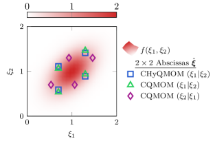
Figure 2: Abscissas $\boldsymbol{\widehat{\xi}}$ corresponding to the number density function example $f$ of section 2.2. Different moment inversion algorithms and permutations are shown for $N_{\widehat{\xi}_{1}}=N_{\widehat{\xi}_{2}}=2$ as labeled.

Figure 2 shows the abscissas for different moment inversion algorithms. Their locations in the internal coordinate space $\boldsymbol{\xi}$ are different, though their weights are such that each quadrature reproduces the exact (up to) second-order moments. We verify that QBMMlib has this property to the carried precision. We discuss the QBMMlib quadrature routines used for this next.

2.3 Moment system closure via quadrature $\mathrm{(}\mathtt{ComputeRHS}\mathrm{)}$

Quadrature approximates the raw moments defined in (3) and required by (5) as

$$\prod_{j=1}^{N_{\boldsymbol{\xi}}}\sum_{i=1}^{N_{\widehat{\xi}_{j}}}\widehat{w}_{j,i}\,\widehat{\xi}_{j,i}^{p_{j}}\to M_{p_{1},\dots,p_{N_{\boldsymbol{\xi}}}}$$ (8)

where $\widehat{\xi}_{j,i}$ (for $i=1,\dots,N_{\widehat{\xi}_{j}}$) are the abscissa for internal coordinate direction $\xi_{j}$ (for $j=1,\dots,N_{\boldsymbol{\xi}}$). These quadrature approximations build $\vec{\bm{F}}$ of (5) (F) via the QBMM function ComputeRHS. ComputeRHS approximates (via quadrature) and sums the required moments (exps) and their coefficients (coefs) for each moment index (momidx). The code snippet below shows this implementation in QBMMlib.

• F = ComputeRHS[w,xi,momidx,               {coefs,exps}];

2.4 Realizable time integration $\mathrm{(}\mathtt{Project}\mathrm{)}$

Stable and realizable time integration of (4) requires recasting the moment set $\vec{\bm{M}}$ from its weights and abscissas [13]. QBMMlib function Project performs this projection. A time integrator (e.g. Euler’s method) then computes the next iteration of the moment set (moments). The code snippet below shows an example QBMMlib projection and Euler time step (with time step size dt).

• momentsP = Project[w,xi,momidx];moments = momentsP + dt F;

QBMMlib also includes an adaptive strong-stability-preserving (SSP) third-order-accurate Runge–Kutta (RK) time integrator, RK23 [45]. The difference between the SSP–RK3 solution an embedded second-order-accurate SSP-RK solution provides a first-order approximation of the time step error. The time step size adjustment is then proportional to this error. The illustrative examples of the next section use this adaptive time stepping procedure.

3 Illustrative examples

3.1 Linear harmonic oscillator

The example case of section 2, including 6, is a linear harmonic oscillator. This moment system is linear and thus closed, so it can also verify the solution methods of QBMMlib via comparison to Monte Carlo simulations.

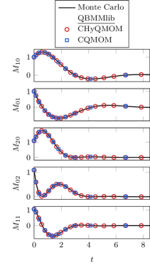
Figure 3: Evolution of the first- and second-order moments in time $t$ for the linear harmonic oscillator example problem. Monte Carlo simulation serves as the truth and the symbols show QBMMlib solutions using $N_{\widehat{\xi}_{1}}=N_{\widehat{\xi}_{2}}=2$ CHyQMOM and CQMOM.

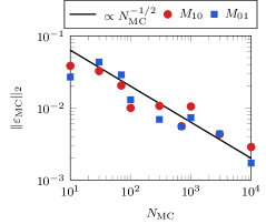
Figure 4: Nominal differences $\lVert\varepsilon_{\text{MC}}\rVert_{2}$ between the first-order moments of Monte Carlo simulation ensembles (of size $N_{\text{MC}}$) and the approximations of CHyQMOM (via QBMMlib). The expected convergence power law $\lVert\varepsilon_{\text{MC}}\rVert_{2}\propto 1/\sqrt{N_{\text{MC}}}$ is also shown.

Figure 3 shows the evolution of CQMOM and CHyQMOM moment sets and compares them to Monte Carlo surrogate truth solutions. The behavior of the first-order moments ($M_{10}$ and $M_{01}$) match the positions and velocities expected of a linear oscillator. Further, the QBMMlib solutions match the moments of the Monte Carlo simulations to plotting accuracy. The $L_{2}$ norm $\lVert\cdot\rVert_{2}$ of the error quantifies this matching as

$$\varepsilon_{\text{MC}}(t)\equiv\frac{M_{ij}^{\text{(MC)}}(t)-M_{ij}^{\text{(QBMM)}}(t)}{\max_{t}M_{ij}^{\text{(QBMM)}}(t)}$$ (9)

where superscripts (MC) and (QMOM) are correspond to Monte Carlo and QBMMlib simulations, respectively. Figure 4 shows $\lVert\varepsilon_{\text{MC}}\rVert_{2}$ for varying Monte Carlo ensemble size $N_{\text{MC}}$ and QBMMlib method CHyQMOM, though the Monte Carlo moment errors dominate the QBMM ones and so CQMOM has the same results. Indeed, the error converges at the expected rate.

3.2 Bubble cavitation

The dynamics of a cavitating gas bubble dispersion serves as a two-internal-coordinate nonlinear example problem. The Rayleigh–Plesset equation models the bubble dynamics [46]:

$$R\ddot{R}+\frac{3}{2}\dot{R}^{2}+\frac{4}{\mbox{Re}}\frac{\dot{R}}{R}=\frac{1}{R^{3}}-C_{p},$$ (10)

where $R$ is the bubble radius, Re is the Reynolds number (dimensionless ratio of inertial to viscous effects), and $C_{p}$ is the dimensionless pressure ratio between the suspending fluid and bubbles. Thus, $R$ and $\dot{R}$ are the two internal coordinates ($\boldsymbol{\xi}$). For our purposes it suffices to ignore surface tension effects (following (10)) and use $C_{p}=1/0.3$ to represent a relatively large pressure ratio. This formulation is non-dimensionalized by the (monodisperse) equilibrium bubble radius and suspending fluid density and pressure. The initial NDF is a log-normal distribution in the $R$-coordinate (shape parameters $\mu_{R}=1,\sigma_{R}=0.2$) and a normal distribution in the $\dot{R}$ coordinate ($\mu_{\dot{R}}=0$, $\sigma_{\dot{R}}=0.1$). The NDF is initially uncorrelated.

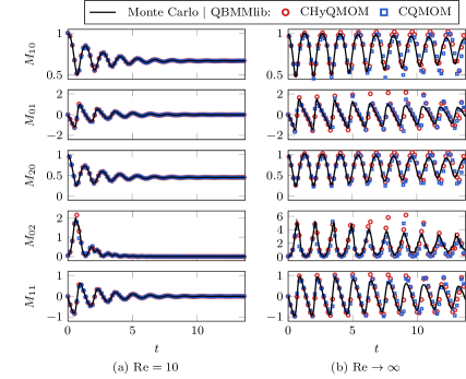
Figure 5: Evolution of the first- and second-order moments for (a) viscous and (b) inviscid bubble dynamics as labeled. Exact moments are approximated by a (sufficiently well converged) $N_{\text{MC}}=5000$ Monte Carlo simulation. The symbols show QBMMlib solutions for $N_{\widehat{\xi}_{1}}=N_{\widehat{\xi}_{2}}=2$ CHyQMOM and CQMOM, as labeled.

Figure 5 shows the moment dynamics for two bubble dispersions problems: (a) viscous $\mbox{Re}=10$ and (b) inviscid $\mbox{Re}\to\infty$. Here, $\mbox{Re}=10$ is the Reynolds number that corresponds to $1\text{\,}\mathrm{\SIUnitSymbolMicro m}$ bubbles in water and $\mbox{Re}\to\infty$ represents ignoring viscous effects. Invoking $\mbox{Re}\to\infty$ is not appropriate for most cavitation problems of physical relevance, though it provides a useful reference. In both cases the mean bubble radius $M_{10}$ oscillates and damps. This damping is more significant in (a) than (b) due to viscous effects, as expected. In the $\mbox{Re}=10$ case, this is sufficient for the QBMMlib-predicted moments to match the Monte Carlo results. However, for $\mbox{Re}\to\infty$, the evolving moment set is unable to faithfully represent the bubble oscillations, particularly at long times. Indeed, a mismatch between the Monte Carlo and QBMMlib results is clear for $M_{02}$ and $M_{11}$. These differences are qualitatively similar for both the CQMOM and CHyQMOM algorithms. This is because closing the moment system requires extrapolating out of the represented moment space, which is of similar fidelity for both algorithms.

4 Impact and conclusions

This paper introduced QBMMlib, a library for solving PBEs using quadrature-based moment methods. It is a Wolfram Language package, which is useful for automating the procedure of using QBMMs for simulating phenomena like bubble and particle dynamics. This includes constructing a moment set for a given QBMM, determining the right-hand-side functions corresponding to a governing equation automatically, and inverting the moment set for quadrature points to close the system. These routines leverage Mathematica’s symbolic algebra features and include modern QMOM and conditional-QMOM methods. Having these features available in a unified framework is helpful, particularly when it is unclear what QBMM will be appropriate (or stable) for the model dynamics. Our searches suggest that QBMMlib is the only library, open source or otherwise, that provides such capabilities. Given this, QBMMlib should help researchers prototyping QBMMs for their physical problems (or developing new QBMMs entirely). Indeed, the authors used QBMMlib to guide the implementation of CHyQMOM for phase-averaged bubble cavitation into MFC, the first flow solver with this capability [47, 48].

Conflict of Interest

We wish to confirm that there are no known conflicts of interest associated with this publication and there has been no significant financial support for this work that could have influenced its outcome.

Acknowledgements

The authors appreciate the insights of Professor Alberto Passalacqua when developing this library. The US Office of Naval Research supported this work under grant numbers N0014-17-1-2676 and N0014-18-1-2625.

References

- Ramkrishna [2000] D. Ramkrishna, Population Balances, Academic Press, New York, USA, 2000.
- Chapman et al. [1990] S. Chapman, T. G. Cowling, D. Burnett, The mathematical theory of non-uniform gases: An account of the kinetic theory of viscosity, thermal conduction and diffusion in gases, Cambridge University Press, 1990.
- Vanni [2000] M. Vanni, Approximate population balance equations for aggregation breakage processes, J. Colloid Interface Sci. 221 (2000) 143–160.
- Smoluchowski [1916] M. Smoluchowski, Über brownsche molekularbewegung unter einwirkung äußerer kräfte und deren zusammenhang mit der verallgemeinerten diffusionsgleichung, Annalen der Physik 353 (1916) 1103–1112.
- Solsvik and Jakobsen [2015] J. Solsvik, H. A. Jakobsen, The foundation of the population balance equation: A review, J. Disp. Sci. Tech. 36 (2015) 510–520.
- Buffo et al. [2012] A. Buffo, M. Vanni, D. Marchisio, Multidimensional population balance model for the simulation of turbulent gas–liquid systems in stirred tank reactors, Chem. Eng. Sci. 70 (2012) 31–44.
- Buffo et al. [2013] A. Buffo, M. Vanni, D. L. Marchisio, R. O. Fox, Multivariate quadrature-based moments methods for turbulent polydisperse gas–liquid systems, Int. J. Multiph. Flow 50 (2013) 41–57.
- Liao et al. [2014] Y. Liao, D. Lucas, E. Krepper, Application of new closure models for bubble coalescence and breakup to steam–water vertical pipe flow, Nucl. Eng. Des. 279 (2014) 126 – 136.
- Li et al. [2017] D. Li, Z. Gao, A. Buffo, W. Podgorska, D. L. Marchisio, Droplet breakage and coalescence in liquid–liquid dispersions: Comparison of different kernels with EQMOM and QMOM, AIChE J. 63 (2017) 2293–2311.
- Gao et al. [2016] Z. Gao, D. Li, A. Buffo, W. Podgórska, D. L. Marchisio, Simulation of droplet breakage in turbulent liquid–liquid dispersions with CFD-PBM: Comparison of breakage kernels, Chem. Eng. Sci. 142 (2016) 277–288.
- Fox [2008] R. O. Fox, A quadrature-based third-order moment method for dilute gas–particle flows, J. Comp. Phys. 227 (2008) 6313–6350.
- Desjardins et al. [2008] O. Desjardins, R. O. Fox, P. Villedieu, A quadrature-based moment method for dilute fluid-particle flows, J. Comp. Phys. 227 (2008) 2514–2539.
- Nguyen et al. [2016] T. T. Nguyen, F. Laurent, R. O. Fox, M. Massot, Solution of population balance equations in applications with fine particles: Mathematical modeling and numerical schemes, J. Comp. Phys. 325 (2016) 129–156.
- Kong and Fox [2017] B. Kong, R. O. Fox, A solution algorithm for fluid–particle flows across all flow regimes, J. Comp. Phys. 344 (2017) 575–594.
- Kazakov and Frenklach [1998] A. Kazakov, M. Frenklach, Dynamic modeling of soot particle coagulation and aggregation: Implementation with the method of moments and application to high-pressure laminar premixed flames, Combust. Flame 114 (1998) 484–501.
- Balthasar and Kraft [2003] M. Balthasar, M. Kraft, A stochastic approach to calculate the particle size distribution function of soot particles in laminar premixed flames, Combust. Flame 133 (2003) 289–298.
- Pedel et al. [2014] J. Pedel, J. N. Thornock, S. T. Smith, P. J. Smith, Large eddy simulation of polydisperse particles in turbulent coaxial jets using the direct quadrature method of moments, Int. J. Multiph. Flow 63 (2014) 23–38.
- Mueller et al. [2009] M. E. Mueller, G. Blanquart, H. Pitsch, A joint volume-surface model of soot aggregation with the method of moments, Proc. Combust. Inst. 32 I (2009) 785–792.
- Sibra et al. [2017] A. Sibra, J. Dupays, A. Murrone, F. Laurent, M. Massot, Simulation of reactive polydisperse sprays strongly coupled to unsteady flows in solid rocket motors: Efficient strategy using Eulerian multi-fluid methods, J. Comp. Phys. 339 (2017) 210–246.
- Laurent and Massot [2001] F. Laurent, M. Massot, Multi-fluid modelling of laminar polydisperse spray flames: Origin, assumptions and comparison of sectional and sampling methods, Combust. Theor. Model. 5 (2001) 537–572.
- Hussain et al. [2015] M. Hussain, J. Kumar, E. Tsotsas, A new framework for population balance modeling of spray fluidized bed agglomeration, Particuology 19 (2015) 141–154.
- Ando et al. [2011] K. Ando, T. Colonius, C. E. Brennen, Numerical simulation of shock propagation in a polydisperse bubbly liquid, Int. J. Multiph. Flow 37 (2011) 596–608.
- Bryngelson et al. [2019] S. H. Bryngelson, K. Schmidmayer, T. Colonius, A quantitative comparison of phase-averaged models for bubbly, cavitating flows, Int. J. Multiph. Flow 115 (2019) 137–143.
- Hulburt and Katz [1964] H. M. Hulburt, S. Katz, Some problems in particle technology: A statistical mechanical formulation, Chem. Eng. Sci. 19 (1964) 555–574.
- Moyal [1949] J. E. Moyal, Stochastic processes and statistical physics, J. Roy. Stat. Soc. B 11 (1949).
- McGraw [1997] R. McGraw, Description of aerosol dynamics by the quadrature method of moments, Aerosol Sci. Technol. 27 (1997) 255–265.
- Wheeler [1974] J. C. Wheeler, Modified moments and Gaussian quadratures, Rocky Mt. J. Math. 4 (1974) 287–296.
- Yuan et al. [2012] C. Yuan, F. Laurent, R. O. Fox, An extended quadrature method of moments for population balance equations, J. Aerosol Science 51 (2012) 1–23.
- Patel et al. [2017] R. G. Patel, O. Desjardins, B. Kong, J. Capecelatro, R. O. Fox, Verification of Eulerian–Eulerian and Eulerian–Lagrangian simulations for turbulent fluid–particle flows, AIChE J. 63 (2017) 5396–5412.
- Kong et al. [2017] B. Kong, R. O. Fox, H. Feng, J. Capecelatro, R. Patel, O. Desjardins, Euler–Euler anisotropic Gaussian mesoscale simulation of homogeneous cluster-induced gas–particle turbulence, AIChE J. 63 (2017) 2630–2643.
- Fox et al. [2018] R. O. Fox, F. Laurent, A. Vié, Conditional hyperbolic quadrature method of moments for kinetic equations, J. Comput. Phys. 365 (2018) 269–293.
- Marchisio and Fox [2005] D. L. Marchisio, R. O. Fox, Solution of population balance equations using the direct quadrature method of moments, J. Aerosol Sci. 36 (2005) 43–73.
- Fox [2003] R. O. Fox, Computational models for turbulent reacting flows, Cambridge University Press, 2003.
- Fox [2006] R. O. Fox, Bivariate direct quadrature method of moments for coagulation and sintering of particle populations, J. Aerosol Science 37 (2006) 1562–1580.
- Marchisio and Fox [2013] D. L. Marchisio, R. O. Fox, Computational models for polydisperse particulate and multiphase systems, Cambridge University Press, 2013.
- Yuan and Fox [2011] C. Yuan, R. O. Fox, Conditional quadrature method of moments for kinetic equations, J. Comput. Phys. 230 (2011) 8216–8246.
- Patel et al. [2019] R. G. Patel, O. Desjardins, R. O. Fox, Three-dimensional conditional hyperbolic quadrature method of moments, J. Comp. Phys. X 1 (2019) 100006.
- Passalacqua et al. [2018] A. Passalacqua, F. Laurent, E. Madadi-kandjani, J. C. Heylmun, R. O. Fox, An open-source quadrature-based population balance solver for OpenFOAM, Chem. Eng. Sci. 176 (2018) 306–318.
- Passalacqua et al. [2019] A. Passalacqua, J. Heylmun, M. Icardi, E. Madadi, P. Bachant, X. Hu, OpenQBMM 5.0.1 for OpenFOAM 7, Zenodo, 2019.
- Weller et al. [1998] H. G. Weller, G. Tabor, H. Jasak, C. Fureby, A tensorial approach to computational continuum mechanics using object-oriented techniques, Comput. Phys. 12 (1998) 620–631.
- Fan et al. [2004] R. Fan, D. L. Marchisio, R. O. Fox, Application of the direct quadrature method of moments to polydisperse gas–solid fluidized beds, Powder Tech. 139 (2004) 7–20.
- Davies et al. [2011] D. R. Davies, C. R. Wilson, S. C. Kramer, Fluidity: A fully unstructured anisotropic adaptive mesh computational modeling framework for geodynamics, Geochem. Geophys. Geosys. 12 (2011).
- Bryngelson et al. [2020] S. H. Bryngelson, A. Charalampopoulos, T. P. Sapsis, T. Colonius, A Gaussian moment method and its augmentation via LSTM recurrent neural networks for the statistics of cavitating bubble populations, Int. J. Multiph. Flow 127 (2020) 103262.
- Fox [2009] R. O. Fox, Optimal moment sets for multivariate direct quadrature method of moments, Industrial and Engineering Chemistry Research 48 (2009) 9686–9696.
- Gottlieb et al. [2011] S. Gottlieb, D. Ketcheson, C.-W. Shu, Strong stability preserving Runge–Kutta and multistep time discretizations, World Scientific, 2011.
- Brennen [1995] C. E. Brennen, Cavitation and bubble dynamics, Oxford University Press, 1995.
- Zhang and Prosperetti [1994] D. Z. Zhang, A. Prosperetti, Ensemble phase-averaged equations for bubbly flows, Phys. Fluids 6 (1994).
- Bryngelson et al. [2020] S. H. Bryngelson, K. Schmidmayer, V. Coralic, J. C. Meng, K. Maeda, T. Colonius, MFC: An open-source high-order multi-component, multi-phase, and multi-scale compressible flow solver, Comp. Phys. Comm. (2020) 107396.