Transfer Learning for Protein Structure Classification at Low Resolution

Abstract

Structure determination is key to understanding protein function at a molecular level. Whilst significant advances have been made in predicting structure and function from amino acid sequence, researchers must still rely on expensive, time-consuming analytical methods to visualise detailed protein conformation. In this study, we demonstrate that it is possible to make accurate ($\geq$80%) predictions of protein class and architecture from structures determined at low ($>$3$\mathrm{\SIUnitSymbolAngstrom}$) resolution, using a deep convolutional neural network trained on high-resolution ($\leq$3$\mathrm{\SIUnitSymbolAngstrom}$) structures represented as 2D matrices. Thus, we provide proof of concept for high-speed, low-cost protein structure classification at low resolution, and a basis for extension to prediction of function. We investigate the impact of the input representation on classification performance, showing that side-chain information may not be necessary for fine-grained structure predictions. Finally, we confirm that high-resolution, low-resolution and NMR-determined structures inhabit a common feature space, and thus provide a theoretical foundation for boosting with single-image super-resolution.

I Introduction

Proteins are large biological molecules consisting of chains of amino acids that are of particular interest to life science research, as they perform a wide variety of essential functions in the cell (Alberts et al., 2007). Functional characterisation of proteins can be arduous, and as such structural biologists can rely on the close relationship between structure and function to predict activity from structure given a known taxonomy of well-characterised protein folds (Whisstock and Lesk, 2003), to complement sequence alignment studies (Eisenhaber, 2000). Broadly speaking, the greater the resolution of a solved structure (given in $\mathrm{\SIUnitSymbolAngstrom}$ngströms, 10^-10m), the more information can be derived from it: individual atoms can be resolved below 1$\mathrm{\SIUnitSymbolAngstrom}$, the polypeptide backbone and amino acid side-chains under 3$\mathrm{\SIUnitSymbolAngstrom}$, and protein backbone conformation at over 3$\mathrm{\SIUnitSymbolAngstrom}$ (Berman et al., 2000), see Fig. 1. The need for atomic resolution is reflected in publication bias, with structures determined at $\leq$3$\mathrm{\SIUnitSymbolAngstrom}$ currently making up 93% of the Protein Data Bank (PDB) (Berman et al., 2000).

Unfortunately, high-resolution structure solving is challenging and represents a fundamental bottleneck in research: to date, more than 120 million amino acid sequences have been determined, but only 160,000 structures have been published (Berman et al., 2000, UniProt, 2015). X-Ray Crystallography (XRC) has historically been the most commonly used technique in protein structure determination, but is time-consuming and expensive: competition for access to facilities is fierce, and costs can reach $100,000 per structure (Stevens, 2003). The requirement for crystallisation also excludes certain protein groups of interest, including some large transmembrane assemblies (Meury et al., 2011). Nuclear Magnetic Resonance (NMR) can yield information not only on topology but on dynamics, but has historically been limited to small soluble proteins (Sugiki et al., 2017). The advent of cryo-Electron Microscopy (cryo-EM) has permitted the visualisation of proteins in near-native conformations at under 2$\mathrm{\SIUnitSymbolAngstrom}$, but the technique remains prohibitively expensive (Peplow, 2017, Hand, 2020).

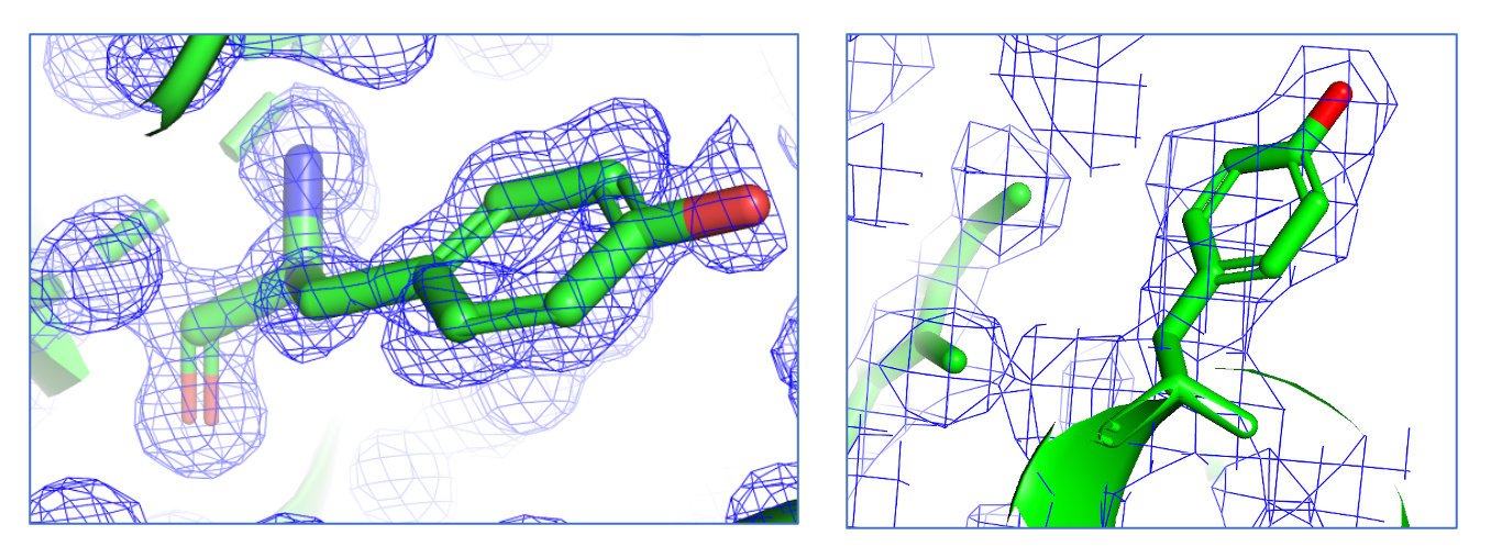
Figure 1: Impact of resolution on structure determination. Myoglobin tyrosine 103 shown from structures 1a6m (1$\mathrm{\SIUnitSymbolAngstrom}$) and 108m (2.7$\mathrm{\SIUnitSymbolAngstrom}$). Electron density displayed as blue cages, atoms shown as sticks. Adapted from PDB 101 (Berman et al., 2000) and produced using pyMol (DeLano, 2020).

As a result, the holy grail of structural biology has become the accurate prediction of protein structure from amino acid sequence alone (Kuhlman and Bradley, 2019). Recent years have seen huge progress in the field, but there remains room for improvement: the best predictors of the most recent Critical Assessment of Structure Prediction competition (CASP13) achieving not more than 80% accuracy in ab initio backbone placement for the most challenging structures (Kryshtafovych et al., 2019). Furthermore, common metrics of predictive accuracy, such as precision of contact prediction, GDT_TS and RMSD, do not take into account amino acid side-chain placement, which is crucial to understanding protein function (Zemla, 2003, Kryshtafovych et al., 2019).

II Problem statement

In light of these challenges, before and if sequence-based structure prediction is solved and/or low-cost, high-resolution imaging becomes widely available, the ability to make accurate predictions of protein structure and function from low-resolution data could feasibly accelerate the pace of research.

Building on previous work (Sikosek, 2019), this project sets out to identify whether the features learned by convolutional neural networks (CNNs) trained on 2D representations of high-resolution structures (defined as $\leq$3$\mathrm{\SIUnitSymbolAngstrom}$) can be used accurately to classify fine-grained protein fold topology from structures determined at low resolution ($>$3$\mathrm{\SIUnitSymbolAngstrom}$). Secondly, we seek to identify which form of input performs best in protein structure classification (PSC), comparing atom selections representative of low, medium and high information content.

III Contribution

We show for the first time that it is feasible to make accurate ($\geq$ 80%) predictions of protein class and architecture from structures solved at low resolution, including a challenging set determined with NMR. In this way, we provide a theoretical basis for mapping between low- and high-resolution structures, and for extension to function prediction. We find that the best predictors are those trained on matrices encoding distances between C_α, C_β, oxygen and nitrogen atoms of the protein backbone (Fig. 2), outperforming heavy atom and alpha carbon selections, and so demonstrate the importance of selecting a representation appropriate to the task. Finally, we achieve benchmark classification performance (89% accuracy) on prediction of homologous superfamily from over 5,150 possible categories, using a four-component ensemble of deep CNNs.

IV Background

IV-A Artificial neural networks (ANNs)

ANNs are a family of machine learning algorithms whose architecture is loosely analogous to the neurons of the mammalian brain, and which have been shown to be powerful predictive tools in disciplines including computer vision and natural language processing (Krizhevsky et al., 2012, Devlin et al., 2019). ANNs are composed of sequential layers of simple computational units (nodes), in which the output of any node is an elementwise combination of its inputs passed through some non-linear activation function (Goodfellow et al., 2016). Given sufficient data, the parameters of these models may be learned via back-propagation in response to a training signal (le Cun, 1988), enabling ANNs to learn arbitrarily complex predictive functions. The more intermediate or ”hidden” layers to a network - deep ANNs having two or more such layers - the more complex the function it can learn, at the cost of greater computational complexity.

IV-B Convolution for image classification and transfer learning

Convolutional neural networks (CNNs) are ANNs containing one or more convolutional layer and which are applied to data with a known grid-like topology, such as images and videos (Goodfellow et al., 2016). The convolution operation allows a layer to scan over its input matrix with a sliding window of stacked nodes (kernels), storing the strongest node outputs in an “activation map” via a pooling operation (LeCun et al., 1990). The power of CNNs in image classification has long been recognised: from Yann LeCun’s work on recognising handwritten digits, to the use of deeper networks and innovative model architectures to label images from the ImageNet repository (LeCun et al., 1990, Krizhevsky et al., 2012, He et al., 2016, Simonyan and Zisserman, 2015). Subsequent work showed that the discriminatory features learned by these models in one image domain (the source) can be transferred to classify data in a separate, noisier or more challenging domain (the target). Examples of such transfer learning approaches include pre-training a network on an image classification task and fine-tuning on a separate object detection task (Razavian et al., 2014), and simultaneous learning between paired high- and low-quality images (Chen et al., 2015).

IV-C Representing proteins as images: protein distance maps

Computational biologists have profited from these advances by converting publicly available three-dimensional protein structures into two-dimensional protein distance maps (hereafter, PDMs): symmetric matrices encoding the pairwise distances between atoms i and j (a_i, a_j) of a solved structure (Phillips, 1970, Hu et al., 2002).

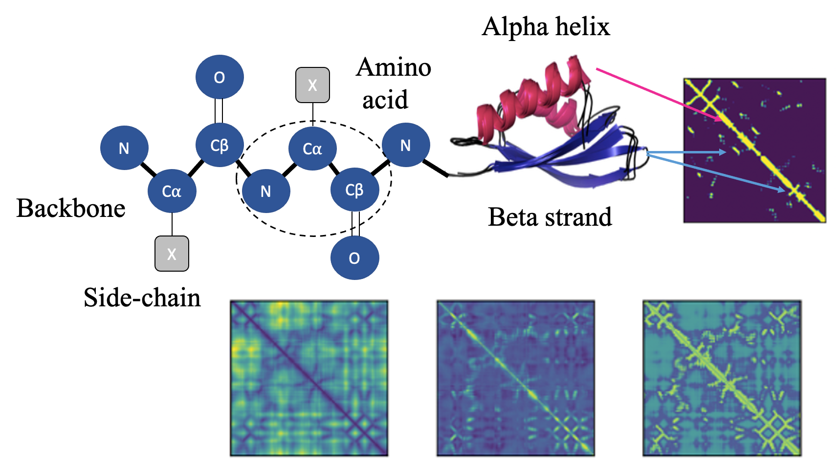
Figure 2: Representing proteins in two dimensions. Top left: Maps may be constructed from distances between the alpha carbon (C_α), beta carbon (C_β), polypeptide backbone (thick black line) or heavy atoms (all non-Hydrogen atoms) of a protein. A single amino acid is shown in the dotted circle. Adapted from (Anand and Huang, 2018). Top centre: Illustrative secondary structure shown from CATH domain 3.30.70.380 (Orengo et al., 1997). Top right: Example contact map. Bottom row (from left to right): Example distance map, anisotropic network model (ANM) and non-bonded (NB) energy matrices (Sikosek, 2019).

PDMs have the advantage over 3D structure representations of reducing both computational load and sensitivity to feature rotation or translation (Sikosek, 2019), and are generally presented in one of two common forms (Fig. 2). Contact maps are binary matrices wherein two atoms are identified as being in contact if they fall within a set distance of one another, typically 7-8$\mathrm{\SIUnitSymbolAngstrom}$ (Duarte et al., 2010). Distance maps directly encode the Euclidean distances between atoms of the protein (De Melo et al., 2006, Pietal et al., 2015). The patterns that appear in these maps correspond to characteristic structural elements, for example alpha helices and beta sheets, as pictured in Fig. 2.

PDMs may be generated from the distances between different selections of atoms, including the alpha (C_α) and/or beta (C_β) carbons of the polypeptide backbone, or the heavy (non-hydrogen) atoms of the backbone and side-chains. The relative merits of different representations remain disputed: Duarte et al. (2010) concluded that a combination of C_α and C_β atoms outperforms individual components (and particularly C_α) when reconstructing 3D protein structures from contact maps, whilst C_α maps performed better than side-chain geometric centres for enzyme class prediction in a study by Da Silveira et al. (2009), and heavy atom representations performed well in a more recent publication from Newaz et al. (2020).

Diverse uses have been found for PDMs in computational biology. Key amongst these are protein structure classification (PSC), as in the present study; retrieval of similar proteins (Liu et al., 2018); as an intermediate step in three-dimensional structure prediction from amino acid sequence (Kuhlman and Bradley, 2019); and even in de novo protein design (Anand and Huang, 2018).

IV-D Related work: Protein structure classification

PSC is the task of assigning a candidate structure to one of a set of discrete three-dimensional patterns (folds) containing the same arrangement and topology of secondary structural elements (Craven et al., 1995). Common reference taxonomies include the class, fold, superfamily and family hierarchies of the structural classification of proteins (SCOP) dataset (Fox et al., 2014), and the class, architecture, fold and homologous superfamily classifications of CATH (Orengo et al., 1997). Notably, PSC may also serve as a convenient objective for producing vector embeddings of protein structures for use in some secondary task (Sikosek, 2019), the implications of which are explored in Section VIII.

A review of the literature was conducted to identify historic approaches to PSC, detailed in Appendix Table AVIII-B. Three broad methodologies were encountered: those in which traditional machine learning algorithms were applied to features extracted from PDMs (Shi and Zhang, 2009, Taewijit and Waiyamai, 2010, Vani and Kumar, 2016, Pires et al., 2011); a second set training deep CNNs directly on large datasets of maps (Sikosek, 2019, Eguchi and Huang, 2020); and ensemble models combining different approaches (Zacharaki, 2017, Newaz et al., 2020). Studies relying on features derived from amino acid sequence alone are not listed exhaustively, however state of the art is included in Table AVIII-B for completeness (Xia et al., 2017, Hou et al., 2018).

Many early PSC studies extracted features from subsets of non-redundant structures labelled according to SCOP class and fold, mining secondary structural features from distance maps using hand-crafted algorithms (Shi and Zhang, 2009, Vani and Kumar, 2016). The best-performing of these (Pires et al., 2011) extracted frequency statistics of C_α distances and applied K-Nearest Neighbour classifier or Random Forest classifiers to these features, achieving 94% on prediction of SCOP family.

Among the best results in CATH classification have been those achieved using deep CNNs (Sikosek, 2019, Eguchi and Huang, 2020) and ensembles (Newaz et al., 2020). A modified version of DenseNet121, capable of simultaneous multi-class, multi-label prediction of CATH categories, demonstrated up to 87% accuracy on the most challenging task, being prediction of homologous superfamily from over 2000 possible classes (Sikosek, 2019). This model was trained on heavy atom distance maps augmented with measures of intrinsic molecular motion and non-bonded energy, as described in (Sikosek, 2019), illustrated in Fig. 2 (bottom row) and detailed below. The resultant model was subsequently used to produce protein fingerprints, efficient feature vectors produced by the penultimate layer of the trained CNN (Fig. 3) and used in a subsequent step as the input to a random forest prediction of a secondary task: small molecule binding activity as measured by ChEMBL.

Eguchi and Huang (2020) deployed a six-layer CNN with up-sampling and deconvolution for semantic segmentation (pixelwise labelling) of C_α distance maps. Applying their model to a CATH non-redundant dataset augmented with cropping and sub-sampled to balance class representation, this group achieved up to 88% per structure accuracy of architecture prediction. It is important to note that the primary aim of the study was not accurate structure-level classification, but rather labelling individual amino acids according to CATH architecture, achieving an impressive average accuracy of 91%.

Newaz et al. (2020) combined models trained on different representations into ensembles for PSC. Among these, distances between the heavy atoms in a protein structure were described as ordered sub-graphs (graphlets), whose frequencies then served as an input feature for logistic regression. This study reported 93%-100% per-class accuracy on CATH homologous superfamily prediction when combining graphlet, sequence and Tuned Gaussian Interval (GIT) representations. It is important to note that only those classes and sub-classes with thirty or more instances were included in the analysis. This permitted a statistically meaningful comparison of different feature inputs and methods; however, the resultant accuracies may not be representative of performance across the universe of possible folds.

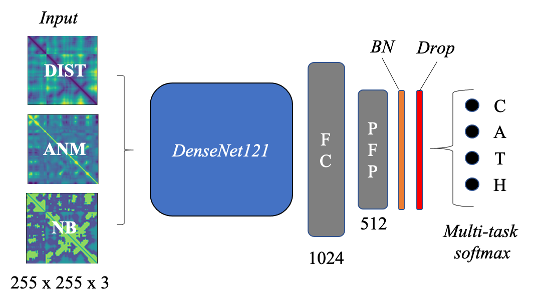
Figure 3: Architecture of the model. Abbreviations. DIST: Distance matrix; ANM: Anisotropic network model; NB: Non-bonded energy; FC: Fully connected (Dense) layer; PFP: protein fingerprint; BN: batch normalisation; Drop: Dropout. Channel depth is shown below the input, FC and PFP layers.

V Methods

V-A Datasets

Protein domains from the CATH non-redundant domain set (v4.2) (Orengo et al., 1997) were assigned to one of three groups according to resolution: “High-resolution” (HR, $\leq$3$\mathrm{\SIUnitSymbolAngstrom}$), “Low-Resolution” (LR, $>$3$\mathrm{\SIUnitSymbolAngstrom}$) and “NMR” (characterised using solution or solid-state NMR). Unlike in previous studies, instances were not excluded on the basis of chain length or a minimum per class frequency, in order to expose the models to as many representative folds as possible. This variance is reflected in the small differences in frequency of T and H classes between datasets (Table A2). The impact of class imbalance on model performance is discussed in VI-A and VIII).

V-B Pre-processing

Structure files from each group were parsed to obtain a stack of distance map, anisotropic network model (ANM) and non-bonded energy (NB) matrices, following (Sikosek, 2019) and described in Algorithm 1. In this way, each image passed to the network encoded information relating to spatial positioning, flexibility and non-bonded energy potentials between each atom of the matrix, respectively.

Initially, PDB files were processed with ABS-PDB2PQR (Jurrus et al., 2018) using an AMBER forcefield, as detailed in Sikosek (2019). Euclidean distance, ANM cross-correlation and NB matrices were then extracted from PQR files for each domain with ProDy (Bakan et al., 2011), using either alpha carbon (CA), backbone (BB) or heavy atom (HEAVY) selections (see Fig. 2 and Algorithm 1). These atom selections were taken to be representative of low, medium and high information content, respectively: CA maps included the distances between C_α atoms only; BB selections including information from C_α, C_β, oxygen and nitrogen; and heavy atom selections including distances between all non-hydrogen atoms, inclusive of side-chains. Summary statistics for each of the nine datasets are provided in Table A2.

Distance matrices were clipped at a maximum distance of 50$\mathrm{\SIUnitSymbolAngstrom}$ (three standard deviations from the mean distance across all maps), and ANM matrices between -1 and +1, before rescaling distance, ANM and NB matrices (in the range [0, 100], [-100, 100] and [-1000, 1000] respectively) for memory-efficient storage. All representations were reshaped with bicubic interpolation and stacked to give a set of 255x255x3-dimensional matrices, comparable to the three channels of RGB colour images.

Algorithm 1 High- to Low-Resolution Domain Transfer

% Extract matrices from structure files %

procedure Parse(domainlist, atomgroup)

    for domainID in domainlist do

         struct $\leftarrow$ parsePQR(pdb2Pqr(domainID))

         atoms $\leftarrow$ selectAtoms(struct, atomgroup)

         ANM $\leftarrow$ ANM(crossCorrelate(atoms))

         charges $\leftarrow$ getCharge(atoms)

         for i in range length(atoms) do

             for j in range length(atoms) do

                 dist[i,j] $\leftarrow$ Euclidean(atoms[i], atoms[j])

                 NB[i,j] $\leftarrow$ getNB(charges[i,j], atoms[i,j])                       

         dist $\leftarrow$ Resize(Clip(dist,0,50),(255,255)*100)

         ANM $\leftarrow$ Resize(Clip(ANM,-1,1),(255,255)*100)

         NB $\leftarrow$ Resize(NB,(255,255)*1000)

         return [dist,ANM,NB], domainID     

    % Train CNN ensemble and return best prediction%

procedure Ensemble(HRInputs, Labels, TestSet)

    for d, Dataset in HRInputs do

         TrainedModel $\leftarrow$ Train(CNN, Dataset, Labels)

         Ensemble[d] $\leftarrow$ TrainedModel     

    w $\leftarrow$ 1$/$ length(Ensemble)

    for model in Ensemble do

         P_test[model] $\leftarrow$ w$*$Predict(model, TestSet)     

    Predicted $\leftarrow$ $\underset{c\in{C},p\in{P}}{\arg\max}$ P_test

    return Predicted

    

% High- to low-resolution domain transfer %

procedure Transfer(HRdomains, TestDomains)

    for atom in CA, BB, HEAVY do

         HRInputs, Labels $\leftarrow$ PARSE(HRDomains, atom)     

    TestSet,TestLabels $\leftarrow$PARSE(TestDomains,atomgroup)

    Predicted $\leftarrow$ ENSEMBLE(HRInputs, Labels, TestSet)

    Accuracy, F1 $\leftarrow$ Evaluate(Predicted,TestLabels)

V-C Model Architecture

Fig. 3 describes the architecture of the deep CNN used in this study, a modified version of pre-trained DenseNet121 from Keras (Chollet, 2015), adapted from (Sikosek, 2019). The final layer of the off-the shelf Keras model was replaced with a single fully-connected protein fingerprint (PFP) layer of 512 dimensions, followed by batch normalisation and dropout layers for regularisation of learned features. The output of these layers was then passed to four parallel softmax activation layers corresponding to the 4 (Class; Task C), 41 (Architecture; Task A), 1391 (Topology; Task T) and 6070 (Homologous Superfamily; Task H) possible categories of the CATH dataset. This framework was adopted with deployment in mind; however, it should be noted that a maximum of 1276/1391 T and 5150/6070 H classes were included in the training set (Table A2). A simple 5-layer CNN was also constructed for comparison, the details of which are included in Fig. A1.

V-D Training

Model training and optimisation studies were performed on one of the three high-resolution datasets (HRCA, HRBB, HRHEAVY), with the aim of maximising test time performance on the most challenging classification task (H). 10% of each high-resolution dataset was retained as a test set for evaluation.

All models were trained to minimise categorical cross entropy loss for a maximum of 150 epochs on a single NVIDIA Tesla T4 GPU, using a 40% validation ratio, shuffled batches of 32 instances and 25% dropout. The initial learning rate was set at 0.001 using an Adam optimiser with no early stopping, and learning rate reduction of 20% enabled after a plateau of 5 epochs, to a minimum of 0.0001.

V-E Evaluation

In order to determine the impact of atom selection on performance, predictive accuracy of models trained on HRCA, HRBB or HRHEAVY datasets was first assessed on held-out test data from the corresponding high-resolution test set, such that a model trained on a high-resolution backbone (HRBB) training set would be evaluated on the HRBB test set. The performance of the best of these models, DenseNet121 trained on HRBB (DN_HRBB) was then evaluated on the high-resolution test sets from other atom selections (HRCA, HRHEAVY) and on the entire low-resolution and NMR datasets (LRCA, LRBB, LRHEAVY, NMRCA, NMRBB and NMRHEAVY).

In addition to accuracy, best model performance was assessed using the F1-score, a harmonic mean of precision and recall that takes account of per-class performance, and the PFP homogeneity score proposed by Sikosek (2019). For the latter, the quality of feature vectors extracted from the PFP layer of trained models (see Fig. 3) was evaluated by clustering instances with K-means (MacQueen, 1967) according to k possible classes for a given task, and comparing the overlap of actual and best predicted label clusters using the homogeneity score functionality of scikit-learn (Pedregosa et al., 2011). Best clusters were identified after 10 iterations following initialisation with kmeans++.

Finally, the best models from each atom selection (DN_HRCA, DN_HRBB and DN_HRHEAVY) were combined into an ensemble (DN_E1), giving each component an equally weighted vote and assigning the most confident weighted prediction as the predicted label, evaluating on all nine test sets. A second four-member ensemble (DN_E2) was also developed that incorporated an additional model trained on distance only HRBB inputs (DN_HRBB_DIST).

VI Results

Average test time accuracy for models trained and tested on HRCA, HRBB and HRHEAVY data is presented in Fig. 4 and Table A3. To assess the contribution of ANM and NB layers to model performance, a model was trained on a modified HRBB dataset comprising triplicate stacks of distance matrices, shown in Fig. 4 (HRBB_DIST) and Table A3. Performance of the best (DN_HRBB) model on HR (held-out), LR and NMR test sets for all three atom selections is presented in (Fig. 5 and Table A4). The results of combining the best models into weighted ensembles is presented in (Tables 1, A5 and A6).

VI-A Impact of atom selection on classification performance

Fig. 4 and Table A3 confirm the finding of Sikosek (2019) that model performance overall correlates with complexity of the task for all atom selections, with highest accuracy seen for task C and worst for task H on all test sets. Across all four tasks, models trained on HRBB maps outperformed those trained on HRCA and HRHEAVY atom selections. For task H, inspection of 95% confidence intervals showed this difference to be statistically significant in both cases (mean accuracy of 67% for HRBB, p$<$0.05, N=3). Average accuracy was numerically lower for HRHEAVY (61%) than HRCA (63%) atom selections, but not significantly so. F1 scores (Table A3) followed a similar trend, but were generally 1-4% lower than the corresponding accuracies, indicating an adverse impact on model performance of class imbalance (detailed in Table A7).

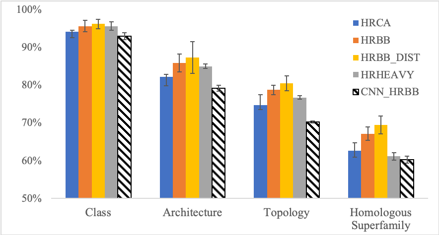
Figure 4: Mean accuracy of models trained and tested on HRCA, HRBB, or HRHEAVY datasets. Error bars show 95% confidence interval. CA: Alpha carbon; BB: Backbone; BB_DIST: triplicate stack of distance matrices; HEAVY: heavy atom selection; CNN_HRBB: CNN comparator, see Fig A1.

TABLE 1: Best performance for DN_HRBB, DN_E1 and DN_E2

Dataset	DN_HRBB				DN_E1				DN_E2
	C	A	T	H	C	A	T	H	C	A	T	H
HRCA	98%	92%	89%	84%	96%	92%	90%	84%	96%	92%	90%	84%
HRBB	96%	86%	79%	81%	94%	90%	86%	80%	96%	93%	92%	89%
HRHEAVY	56%	26%	16%	1%	94%	76%	63%	58%	94%	76%	63%	58%
LRCA	93%	80%	67%	51%	90%	80%	69%	53%	81%	54%	44%	39%
LRBB	92%	79%	64%	48%	87%	78%	66%	49%	79%	52%	42%	37%
LRHEAVY	38%	13%	9%	1%	89%	64%	50%	43%	29%	3%	40%	40%
NMRCA	91%	79%	63%	46%	88%	80%	65%	47%	78%	56%	39%	33%
NMRBB	91%	79%	61%	44%	86%	79%	62%	44%	83%	57%	41%	34%
NMRHEAVY	38%	7%	3%	1%	88%	64%	46%	36%	28%	6%	38%	32%
Comparators
Benchmark (Sikosek, 2019)	99%	95%	92%	87%
CNN_HRBB	93%	79%	70%	60%
DN_HRBB: DenseNet121 trained on HRBB; DN_E1: Ensemble 1; DN_E2: Ensemble 2; CNN_HRBB: CNN comparator,
see Fig A1. Best performers are underlined for HR (DN_E2), LR (DN_E1) and NMR (DN_E1) test sets.

Replacing the ANM and NB layers of HRBB instances with copies of the distance matrix layer improved average accuracy marginally across tasks when compared with a distance-ANM-NB stack (Fig. 4 and Table A3). However, this improvement (69% vs. 67% for task H) was not found to be statistically significant.

When evaluating trained models on task H with held-out high-resolution data (Fig. 5, Tables 1 and A4), the best (DN_HRBB) model performed better on the HRCA dataset (84% for task H) than on HRBB data (81%), and was unable to make predictions from HRHEAVY data (1%). The former figures compare well with 87% accuracy in the benchmark study (Sikosek, 2019), despite having markedly more classes to choose from (5,150 vs 2,714, Table AVIII-B). A 5-layer CNN, trained and tested on HRBB data (CNN_HRBB, Fig. A1), performed worse than the average for corresponding DN_HRBB model across all tasks.

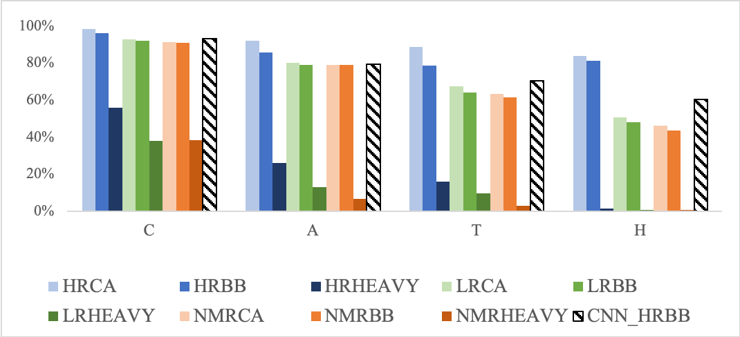
Figure 5: Accuracy of DN_HRBB on C, A, T and H tasks across test sets. CNN_HRBB: CNN comparator.

PFP homogeneity correlated broadly with accuracy and F1 scores for the high-resolution test sets: learned embeddings produced by DN_HRBB form clusters close to their true labels when provided with inputs from HRCA (84% homogeneity for task C) and HRBB (83%) datasets, but not for HRHEAVY (0%) (Table A4). PFP homogeneity was consistently lower for the present study when compared with benchmark experiments (Sikosek, 2019), but followed a similar trend across tasks.

Application of a random forest classifier to the 512-dimensional protein fingerprints produced by DN_HRBB from each test set did not improve classification performance compared to DenseNet121 alone (Table A8).

VI-B Performance of trained models on low-resolution and NMR datasets

The best-performing single model (DN_HRBB) is able to make predictions of over 91%, 79%, 63% and 46% for class, architecture, topology and homologous superfamily across LRCA and NMRCA datasets (Fig. 5 and Table A4). Predictions were consistently better for LR than for NMR datasets across all test sets. As for HR test sets, performance of DN_HRBB was better for CA than for BB test sets, and was very poor (1%) for heavy atom selections. Accuracy and F1 scores corresponded very closely for these analyses, and PFP homogeneity scores followed a similar trend to those observed for tests on HR datasets (Table A4). Any attempts to fine-tune trained models for improved performance on low-resolution or NMR datasets led to loss of performance.

VI-C Ensemble models

A mixed ensemble of HRCA, HRBB and HRHEAVY models (DN_E1) is able to make task H predictions from HR, LR and NMR data that are similar to or better than the best HRBB-only model across all classes and atom selections (Tables 1 and A5). Inclusion of both mixed (distance, ANM and NB) and distance-only representations (model DN_E2, Tables 1 and A6) improved performance on the HR datasets - up to 89% accuracy on HRBB (87% F1) - but damaged predictions on the LR and NMR test sets when compared with E1.

VII Discussion

VII-A Models trained on backbone selections outperform those trained on alpha carbon or heavy atoms

DN_HRBB achieved up to 84% accuracy in homologous superfamily prediction on high-resolution test sets (Tables 1 and A4). This compares well not only with benchmark CATH prediction accuracy from distance maps (87%, over fewer classes), but with sequence-dependent prediction algorithms such as DeepSF, which achieved 75% test accuracy on the 1175 folds of SCOP1.75 (Hou et al., 2018) (Table AVIII-B).

Models trained on HRBB data performed better than HRCA or HRHEAVY equivalents (Fig. 4 and Table A3) when testing on held-out data from the same high-resolution dataset. This is unsurprising when comparing backbone representations with the more compact C_α representations, and falls in line with the findings of Duarte et al. (2010). One might expect models trained on heavy atom selections to perform better, as they contain additional information on the relative spatial orientation of side-chain atoms in addition to the carbon, oxygen and nitrogen atoms of the polypeptide backbone (Fig. 2). However, this information is not necessarily required for CATH classification, which is defined using secondary structural characterisation (topology of the backbone), combined with functional annotation using SwissProt (Orengo et al., 1997). As an additional benefit, HRBB representations occupy on average 20% of the memory of HRHEAVY equivalents before pre-processing (Table A2).

The comparative reduction in performance between HRBB and HRHEAVY-trained models could possibly be attributed to loss of representative images during parsing from PDB source structures (HRHEAVY contains 1,932 fewer training instances). An alternative explanation is information loss during rescaling, the average matrix containing 1,234 atoms for heavy and 635 atoms for BB datasets (Table A2). Reshaping matrices to 255x255 therefore imposes a 23- and 6-fold reduction in area, respectively, compared with a 3-fold upscale for CA instances.

VII-B Complex representations may not be required for accurate fold classification

Ablation experiments that removed the ANM and NB layers of the input representation did not significantly impact the point accuracy of predictions made when compared with a distance-ANM-NB stack, but did seem to increase the variance of both accuracy and F1 (Table A3). This implies that the distance matrix plays a dominant role in model training, but that a more varied input may result in improvements to the diversity (and so robustness) of learned features, as illustrated in the domains triggering maximal activation in the first layer (Fig. A2).

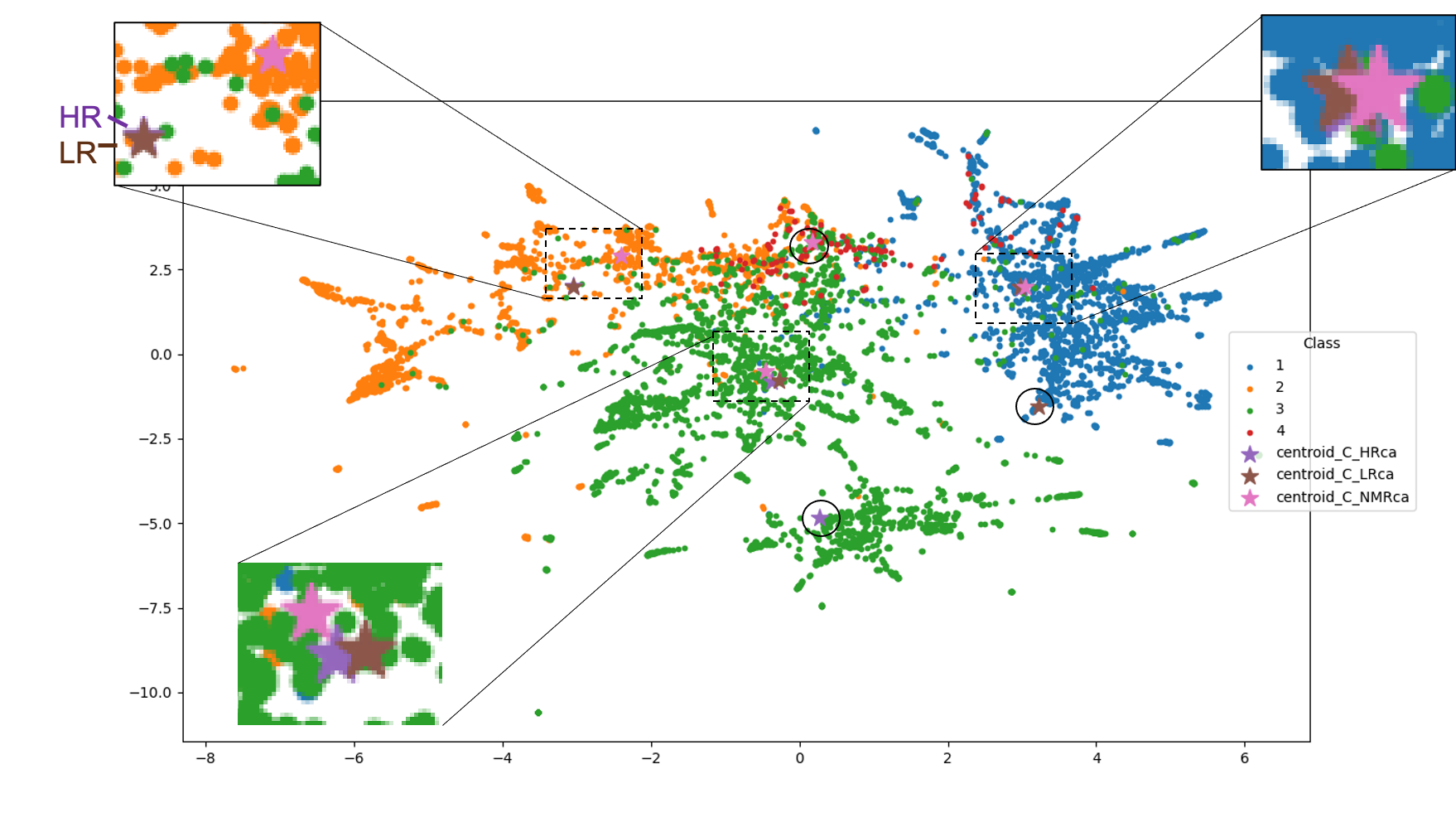
Figure 6: Co-localisation of cluster centroids for HR, LR and NMR datasets. Coloured dots: instances consolidated from HR, LR and NMR datasets and coloured according to class. Stars: cluster centroids. Black circles: misplaced centroids for class 4.

DN_HRBB is able to make more accurate predictions from HRCA than from HRBB data (84% vs. 81%, Fig. 5, Tables 1 and A4). This suggests a shared feature space between the two datasets, presumably the relative position of the alpha carbons in the C_α, C_β, O, N repeating unit of the polypeptide backbone. This signifies that one can train the classifier using (BB) representations of intermediate complexity, and deploy on compact (CA) representations whilst simultaneously improving performance. The same is not true of heavy atom selections, where performance of HRBB drops to 1% (Table 1), possibly as the inclusion of side-chain distances masks the distinctive signals between C_α and C_β atoms. Whilst side-chain information might not be required for accurate CATH classification, it may be useful where learned embeddings are transferred to some secondary task such as prediction of functional site location (Buturovic et al., 2014), small molecule binding (Sikosek, 2019) or structure retrieval (Liu et al., 2018). Heavy atom selections should therefore not be discounted until the relationship between the input representation and the training objective is fully characterised.

VII-C Models trained on HR data can be used to make fold predictions from LR and NMR data

As expected from results with high-resolution data, DN_HRBB performance is better for C, A and T than for H tasks for both low-resolution and NMR datasets. For C and A tasks in particular, accuracies are only marginally worse than seen for the HR test sets (Fig 5) and are improved further using ensembles (Table 1). Whilst one might expect reasonably accurate predictions from structures determined at 3-4$\mathrm{\SIUnitSymbolAngstrom}$ as in the LR datasets (Table A2), the performance of the classifier on NMR structures is more surprising where, as a non-diffraction method, resolution is commonly low ($>$4$\mathrm{\SIUnitSymbolAngstrom}$) or unspecified (999$\mathrm{\SIUnitSymbolAngstrom}$). Further, the nature of the atomic coordinates differs, being an average over an ensemble of possible structures for NMR, and a point estimate based on electron density for XRC and cryo-EM stuctures (Berman et al., 2000).

The ability of the trained model accurately to predict protein class and architecture from LR and NMR test sets is likely attributable to shared patterns of interatomic distances between datasets. To test this hypothesis, 512-dimensional protein fingerprints produced by DN_HRBB were compared for HRCA, LRCA and NMRCA test sets, by computing cluster centroids (class-specific averages) using K-means, and transforming the resultant vectors into two dimensions with t-SNE (Van Der Maaten and Hinton, 2008), shown in Fig. 6.

Comparing the distribution of transformed embeddings (dots, all datasets combined) and centroids (stars, cluster averages for individual datasets) shows that HRCA, LRCA and NMRCA centroids co-localise for classes 1-3 (mainly $\alpha$, mainly $\beta$, and $\alpha$-$\beta$) but not for class 4 (few secondary structures). For the dominant classes (1-3), HR (purple) and LR (brown) centroids are generally closer together, and NMR centroids (pink) are close to but generally separate from HR/LR equivalents. The latter may reflect the different methodology for structure determination by NMR, or the composition of proteins suitable for this technique, being generally small (an average of 94 residues, Table A2) and soluble (Berg JM, Tymoczko JL, 2002). Class 4 instances (shown in red) are underrepresented and exhibit significant overlap with classes 1-3: The K-means algorithm therefore fails to identify them as a discrete cluster (centroids in black circles). This is perhaps unsurprising as the minor class is made up of irregular domains with little secondary structure (Orengo et al., 1997). Class imbalance and overlap for class 4 is reflected in weighted average F1 scores (52% vs. 94%-97%, Table A7).

VII-D A multi-model ensemble achieves benchmark performance on high-resolution datasets

A weighted ensemble (DN_E2) of models is able not only to outperform single model-equivalents (Table 1), but achieves 89% accuracy (87% F1) on class H prediction from HRBB data, a marginal improvement on the benchmark (Sikosek, 2019). Comparing the results achieved for DN_E1 and DN_E2 illustrates that ensemble components can be tuned to perform on different tasks and input representations, DN_E1 performing better on low-resolution data and E2 on high-resolution data (Table 1).

VIII Limitations and further work

The present study has shown that sequence and side-chain information may not be required for accurate prediction of structure classification at high-resolution. However, it should be noted that PSC often serves as a convenient training objective to produce embeddings as an input for some secondary task, particularly in identifying related domains (Liu et al., 2018), rather than as the primary task per se. A crucial extension of this work is therefore to assess the impact of including side-chain information and/or sequence information on performance in secondary tasks, for example on the ”TAPE” tasks developed by Rao et al. (2019).

Class imbalance is a well-known challenge in protein structure classification (Vani and Kumar, 2016). In previous studies, datasets have been carefully trimmed in order to balance representation, for example by including only those classes with thirty or more representative structures (Newaz et al., 2020). This approach was discounted in the present study, training on all available instances from the CATH non-redundant dataset in order to maximise coverage of the universe of possible classes. As a result, many categories of superfamily are represented by a single domain, and the vast majority (92-98%) of superfamilies contain fewer than ten instances (Table A2). This imbalance generates a risk that trained models not be able correctly to classify new unseen minority class instances, which could be assessed in future studies by testing model performance using other datasets such as SCOP (Fox et al., 2014). Possible techniques to counteract class imbalance include boosting minority representation in the training set with additional structures drawn from PDB, synthetic minority oversampling (SMOTE) as in (Vani and Kumar, 2016), or sub-cropping (Eguchi and Huang, 2020). Other possible avenues to explore include objective function re-weighting (Eguchi and Huang, 2020), weighted ensembles of class-specific models, and minority class incremental rectification (Dong et al., 2019).

We have shown that it is possible to make accurate ($\geq$80%) predictions of protein class (C) and architecture (A) from low-resolution and even NMR data, but that performance drops significantly for the more challenging topology and homologous superfamily tasks. One possible approach to improving performance on low-resolution structures is to integrate representations of the same class obtained using different experimental methods into individual instances, an example of multi-view learning (Zhao et al., 2017).

Finally, the evidence presented confirms that low-resolution and NMR structures inhabit a common feature space with high-resolution data, and so provides a theoretical basis for mapping between the domains using techniques such as single image super-resolution (Dong et al., 2016). Such a mapping could help to overcome the bottleneck in obtaining high-resolution structures and so accelerate the pace of future research into human health and disease.

Appendix

VIII-A Figures

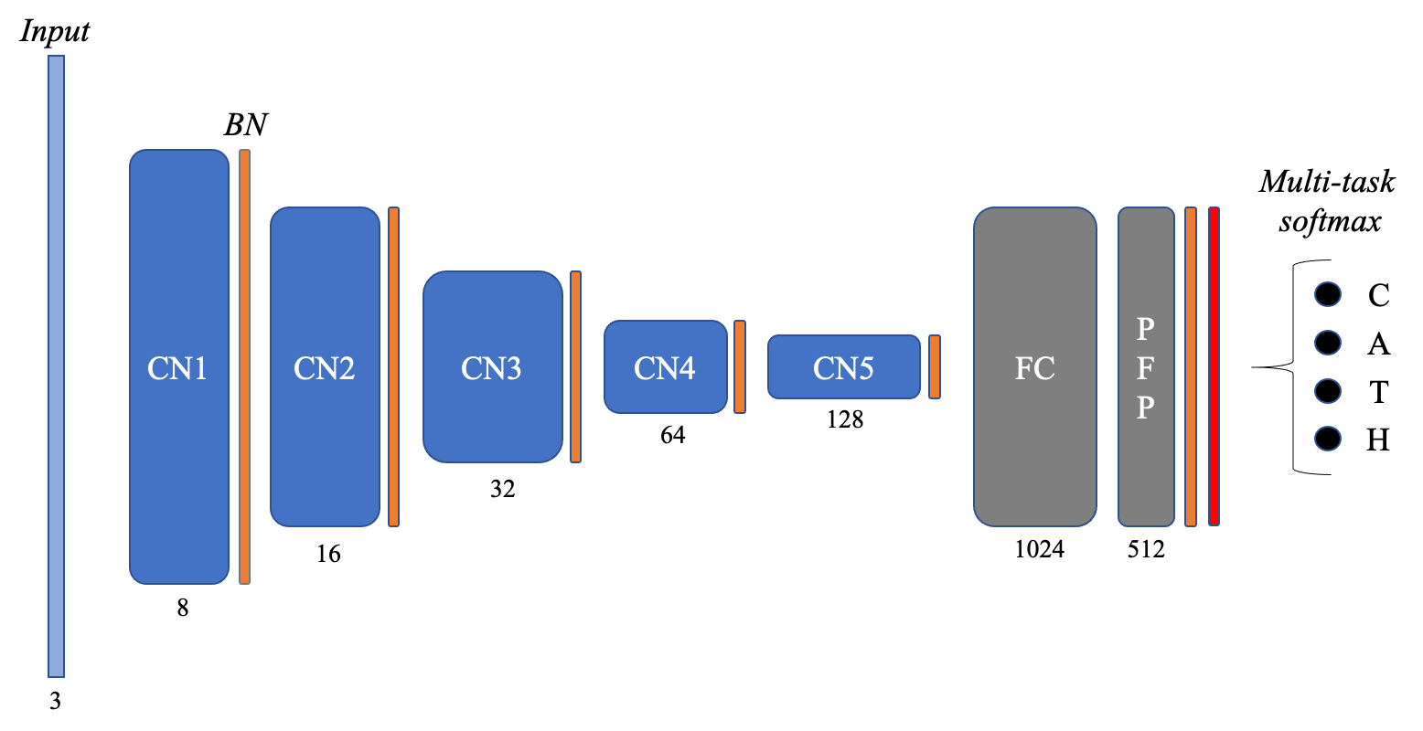
Fig. A 1: CNN Architecture. A simple CNN was prepared in Keras as a comparator for DenseNet121 as pictured above. Convolutional layers were initialised with glorot uniform distribution, and training was carried out on HRBB as specified for DenseNet121 in Section V-D. CN: Convolutional layer; BN: Batch normalisation; FC: Fully connected (Dense) layer; PFP: Protein fingerprint (Dense) layer; Drop: Dropout layer. CN specifications (kernel, stride): CN1 (4,1); CN2 (4,2); CN3&4 (4,4); CN5 (4,2).

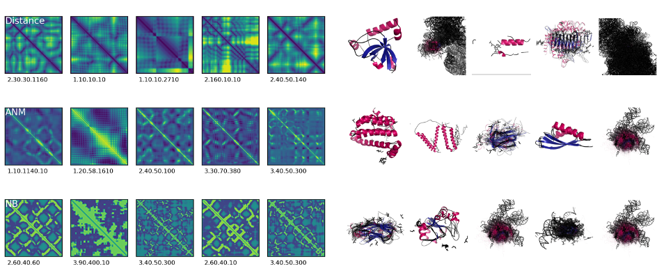
Fig. A 2: Strongest activation maps (left) and corresponding superfamily architectures (right) for distance, ANM and NB layers. Top five activations maps (maximum summed intensity) were extracted for the LRCA dataset from the first layer of DN_HRBB. CATH classifications are shown beneath each activation in the format C.A.T.H. Each channel of the first layer responds maximally to different features and domain families. One exception is superfamily 3.40.50.300 (P-loop containing nucleoside triphosphatases), which appears twice for the NB layer and once for the ANM layer, but not for the distance layer.

VIII-B Tables

Table A 1: Prior art in protein structural classification

Model	Representation	N	Task	Performance
Traditional machine learning approaches
Shi and Zhang (2009): SVM	Secondary structure features mined from Cα distance maps	313	SCOP	Acc :
			Class (4)	91%
			Fold (27)	51%-75%
Pires et al. (2011): KNN / Random Forest	Cut-off Scanning Matrix + SVD from Cα distance maps		EC	P :
		566	Enzyme superfamily (6)	99%
		55,475	Enzyme subfamily (7)	95%
			SCOP∗
		110,799	Class	95%
		108,332	Fold	92%
		106,657	Superfamily	93%
		102,100	Family	94%
Taewijit and Waiyamai (2010): SVM	HMM sequence embeddings + SCCP mined from Cα contact maps	2,640	Enzyme subfamily (16)	Acc : 73%-79%
Vani and Kumar (2016): C4.5 Decision Tree + SMOTE	Secondary structure features mined from Cα distance maps	330	SCOP fold (27)	F1 : 72%
Deep CNNs
Sikosek (2019): Pre-trained DenseNet121	Heavy atom distances + NB + ANM	20,798	CATH	Acc :
			C (4)	99%
			A (40)	95%
			T (1364)	92%
			H (2714)	87%
Eguchi and Huang (2020): 6-layer CNN with ‘pixel shuffle’ and deconvolution	Cα distance maps	126,069	CATH: A (40)	Acc : 88%
Ensembles
Zacharaki (2017): Deep CNN ensemble + SVM/KNN	Amino acid torsion angles + Cα distance maps	44,661	Enzyme superfamily (6)	Acc : 90%
Newaz et al. (2020): Logistic regression	Protein structure networks (heavy atoms $\leq$6$\mathrm{\SIUnitSymbolAngstrom}$) + sequence + GIT (“Concatenate”)	9,440	CATH	Acc :
			C (3)	94%
			A (10)	87%-90%
			T (14)	88%-99%
			H (5)	93%-100%
This study: DenseNet121 ensemble	Backbone atom distances + NB + ANM	15,116-17,048	CATH	Acc :
			C (4)	96%
			A (37)	93%
			T (1276)	92%
			H (5150)	89%
Prediction from sequence
Xia et al. (2017): SVM + HMM Ensemble	Amino acid sequence	6,451	SCOP	Acc : 91%
			Fold (184)
Hou et al. (2018): Deep 1D CNN	Amino acid sequence	15,956	SCOP	Acc : 75%
			Fold (1,195)
Abbreviations. Methods: ANM: Anisotropic Network Model; GIT: tuned Gauss Intervals; HMM: Hidden Markov Model
KNN: K-Nearest Neighbour; NB: Non-bonded energy; SCCP: Sub-Structural Contact Pattern; SMOTE: Synthetic Majority
Oversampling Technique SVD, Single Value Decomposition; SVM, Support Vector Machine; N: total size of dataset. Datasets: CATH:
Class, Architecture, Topology, Homolgous superfamily; EC: Enzyme Classification; SCOP: structural classification of proteins. Metrics:
Acc: Accuracy; F1: F1-score; P: precision.∗Number of categories per class not stated, reference database contains 6, 7, 8 and 24
categories for the four levels of the SCOP hierarchy.

Table A 2: Summary statistics for high-resolution (HR), low-resolution (LR) and NMR datasets

Atom selection	Instances				Classes					Res.∗	Length∗∗	Length∗∗	Size∗∗
	Ntotal	Ntrain	Nval	Ntest	NCC	NCA	NCT	NCH	NCH<10	($\mathrm{\SIUnitSymbolAngstrom}$)	(atoms)	(residues)	(Kb)
High-Resolution ($\leq$3$\mathrm{\SIUnitSymbolAngstrom}$)
HRCA	28,188	15,222	10,148	2,819	4	41	1,276	5,129	91%	2 (1,3)	159	161	35
HRBB	28,412	15,342	10,228	2,841	4	41	1,276	5,150	91%		635	161	167
HRHEAVY	25,192	13,604	9,069	2,519	4	41	1,269	5,002	92%		1234	106	765
Low-Resolution ($>$3$\mathrm{\SIUnitSymbolAngstrom}$)
LRCA	1,663			1,663	4	28	375	885	98%	3 (3,4)	151	153	176
LRBB	1,585	N/A		1,585	4	28	369	859	98%		603	153	176
LRHEAVY	1,633			1,633	4	28	370	873	98%		1,173	153	817
NMR
NMRCA	2,902			2,902	4	26	397	1,045	96%	999 (4,999)	94	92	6
NMRBB	2,872	N/A		2,872	4	26	396	1,039	96%		375	92	52
NMRHEAVY	2,875			2,875	4	26	395	1,036	96%		735	92	238
Abbreviations: CA: alpha carbon; BB: backbone; N: Number of instances; NC: Number of classes; NCH<10: Proportion of H classes having fewer than
ten instances; Res.: Resolution.∗Mean over all instances of the dataset, (min,max), ∗∗ Mean length before pre-processing

Table A 3: Impact of atom selection on model performance

Representation	Ntrain	Ntest	Test Accuracy
			C	A	T	H
HRCA	16,913	2,360	94 $\pm$ 0.4%	82% $\pm$ 0.6%	75% $\pm$ 2.6%	63% $\pm$ 2.2%
HRBB	17,048	2,818	96 $\pm$ 1.5%	86% $\pm$ 2.4%	79% $\pm$ 1.3%	67% $\pm$ 1.7%
HRBB_DIST_ONLY	17,396	2,899	96 $\pm$ 1.2%	87% $\pm$ 4.2%	80% $\pm$ 2.0%	69% $\pm$ 2.4%
HRHEAVY	15,116	2,519	96 $\pm$ 1.1%	85% $\pm$ 0.6%	77% $\pm$ 0.5%	61% $\pm$ 1.0%
CNN_HRBB	17,048	2,818	93 $\pm$ 1.0%	79% $\pm$ 0.8%	70% $\pm$ 0.2%	60% $\pm$ 0.9%
Benchmark (Sikosek, 2019)	12,479	8,319	99%	95%	92%	87%
Representation	Ntrain	Ntest	F1-score
			C	A	T	H
HRCA	16,913	2,360	94 $\pm$ 0.5%	82% $\pm$ 0.5%	73% $\pm$ 3.1%	59% $\pm$ 2.3%
HRBB	17,048	2,818	96 $\pm$ 1.6%	86% $\pm$ 2.6%	77% $\pm$ 1.4%	64% $\pm$ 2.0%
HRBB_DIST_ONLY	17,396	2,899	96 $\pm$ 1.3%	87% $\pm$ 4.5%	80% $\pm$ 2.9%	68% $\pm$ 4.6%
HRHEAVY	15,116	2,519	95 $\pm$ 1.2%	85% $\pm$ 0.5%	75% $\pm$ 0.5%	59% $\pm$ 1.0%
CNN_HRBB	17,048	2,818	93 $\pm$ 0.9%	79% $\pm$ 0.8%	68% $\pm$ 0.1%	57% $\pm$ 1.7%

Table A 4: HRBB performance across test sets

Representation	Ntest	Test Accuracy
		C	A	T	H
High-Resolution ($\leq$3$\mathrm{\SIUnitSymbolAngstrom}$)
HRCA	2,360	98%	92%	89%	84%
HRBB	2,818	96%	86%	79%	81%
HRHEAVY	2,519	56%	26%	16%	1%
Low-Resolution ($>$3$\mathrm{\SIUnitSymbolAngstrom}$)
LRCA	1,663	93%	80%	67%	51%
LRBB	1,585	92%	79%	64%	48%
LRHEAVY	1,634	38%	13%	9%	1%
NMR
NMRCA	3,047	91%	79%	63%	46%
NMRBB	3,017	91%	79%	61%	44%
NMRHEAVY	3,019	38%	7%	3%	1%
Benchmark (Sikosek, 2019)	8,319	99%	95%	92%	87%
Representation	Ntest	F1-score
		C	A	T	H
High-Resolution ($\leq$3$\mathrm{\SIUnitSymbolAngstrom}$)
HRCA	2,360	98%	92%	88%	84%
HRBB	2,818	96%	85%	77%	65%
HRHEAVY	2,519	40%	11%	4%	0%
Low-Resolution ($>$3$\mathrm{\SIUnitSymbolAngstrom}$)
LRCA	1,663	93%	80%	67%	51%
LRBB	1,585	92%	79%	64%	46%
LRHEAVY	1,634	21%	3%	2%	0%
NMR
NMRCA	3,047	91%	79%	63%	46%
NMRBB	3,017	90%	78%	61%	44%
NMRHEAVY	3,019	21%	1%	0%	0%
Representation	Ntest	PFP homogeneity
		C	A	T	H
High-Resolution ($\leq$3$\mathrm{\SIUnitSymbolAngstrom}$)
HRCA	2,360	84%	68%	90%	94%
HRBB	2,818	83%	70%	87%	92%
HRHEAVY	2,519	0%	0%	0%	0%
Low-Resolution ($>$3$\mathrm{\SIUnitSymbolAngstrom}$)
LRCA	1,663	55%	57%	85%	93%
LRBB	1,585	44%	58%	85%	94%
LRHEAVY	1,634	0%	0%	0%	0%
NMR
NMRCA	3,047	50%	61%	82%	90%
NMRBB	3,017	52%	60%	82%	90%
NMRHEAVY	1,634	0%	0%	0%	0%
Benchmark (Sikosek, 2019)	8,319	93%	89%	95%	97%

Table A 5: Test set performance of ensemble DN_E1

Atom selection	Ntest	Accuracy				F1-score
		C	A	T	H	C	A	T	H
High-Resolution ($\leq$3$\mathrm{\SIUnitSymbolAngstrom}$)
HRCA	2,360	96%	92%	90%	84%	96%	92%	89%	82%
HRBB	2,818	94%	90%	86%	80%	94%	90%	86%	77%
HRHEAVY	2,519	94%	76%	63%	58%	93%	76%	61%	57%
Low-Resolution ($>$3$\mathrm{\SIUnitSymbolAngstrom}$)
LRCA	1,663	90%	80%	69%	53%	90%	81%	69%	51%
LRBB	1,585	87%	78%	66%	49%	87%	79%	66%	47%
LRHEAVY	1,634	89%	64%	50%	43%	89%	66%	50%	44%
NMR
NMRCA	3,047	88%	80%	65%	47%	87%	81%	65%	47%
NMRBB	3,017	86%	79%	62%	44%	85%	79%	62%	43%
NMRHEAVY	3,019	88%	64%	46%	36%	87%	69%	51%	39%
BENCHMARK (Sikosek, 2019)	12,479	99%	95%	92 %	87%

Table A 6: Test set performance of ensemble E2

Atom selection	Ntest	Accuracy				F1-score
		C	A	T	H	C	A	T	H
High-Resolution ($\leq$3$\mathrm{\SIUnitSymbolAngstrom}$)
HRCA	2,360	96%	92%	90%	84%	96%	92%	89%	82%
HRBB	2,818	96%	93%	92%	89%	96%	94%	92%	87%
HRHEAVY	2,519	94%	76%	63%	58%	93%	76%	61%	57%
Low-Resolution ($>$3$\mathrm{\SIUnitSymbolAngstrom}$)
LRCA	1,663	81%	54%	44%	39%	81%	57%	52%	42%
LRBB	1,585	79%	52%	42%	37%	79%	54%	51%	39%
LRHEAVY	1,634	29%	3%	40%	40%	13%	4%	47%	42%
NMR
NMRCA	3,047	78%	56%	39%	33%	78%	57%	47%	37%
NMRBB	3,017	83%	57%	41%	34%	82%	56%	48%	37%
NMRHEAVY	3,019	28%	6%	38%	32%	12%	5%	45%	36%
BENCHMARK (Sikosek, 2019)	12,479	99%	95%	92 %	87%

Table A 7: Per category performance of HRBB model on HRBB test set

CATH label	Description	Precision	Recall	F1-score	Support
Class
1	Mainly alpha	97%	96%	97%	655
2	Mainly beta	94%	94%	94%	589
3	Alpha - beta	97%	97%	97%	1554
4	Few secondary structures	50%	55%	52%	20
Architecture
1.10	Orthogonal bundle	86%	90	88	389
1.20	Up-down bundle	82%	74%	78%	206
1.25	Alpha horseshoe	88%	88%	88%	49
1.40	Alpha solenoid	100%	100%	100%	1
1.50	Alpha / alpha barrel	91%	100%	95%	10
2.10	Ribbon	64%	80%	71%	20
2.20	Single sheet	47%	38%	42%	24
2.30	Roll	83%	75%	79%	73
2.40	Beta barrel	84%	86%	85%	137
2.50	Clam	100%	50%	67%	2
2.60	Sandwich	98%	94%	96%	250
2.70	Distorted sandwich	73%	92%	81%	12
2.80	Trefoil	92%	100%	96%	12
2.90	Orthogonal prism	100%	100%	100%	2
2.100	Aligned prism	100%	67%	80%	3
2.102	3-layer sandwich	50%	100%	67%	1
2.105	3 propeller	0%	0%	0%	0
2.110	4 propeller	0%	0%	0%	0
2.115	5 propeller	67%	100%	80%	4
2.120	6 propeller	100%	83%	91%	6
2.130	7 propeller	100%	100%	100%	14
2.140	8 propeller	100%	100%	100%	1
2.150	2 solenoid	100%	100%	100%	1
2.160	3 solenoid	100%	93%	96%	14
2.170	Beta complex	47%	62%	53%	13
2.180	Shell	0%	0%	0%	0
3.10	Roll	76%	70%	73%	105
3.15	Super roll	100%	100%	100%	3
3.20	Alpha-beta barrel	93%	51%	66%	128
3.30	2-layer sandwich	83%	86%	84%	399
3.40	3-layer (aba) sandwich	89%	97%	93%	702
3.50	3-layer (bba) sandwich	100%	89%	94%	28
3.55	3-layer (bab) sandwich	100%	100%	100%	2
3.60	4-layer sandwich	96%	72%	82%	32
3.65	Alpha-beta prism	100%	100%	100%	2
3.70	Box	100%	100%	100%	3
3.75	5-stranded propeller	100%	100%	100%	2
3.80	Alpha-beta horseshoe	100%	91%	95%	11
3.90	Alpha-beta complex	77%	79%	78%	137
3.100	Ribosomal protein L15	0%	0%	0%	0
4.10	Irregular	41%	55%	47%	20%

Table A 8: Applying a Random Forest ensemble to protein fingerprints

Training set	Test set	Ntest	Accuracy
			C	A	T	H
HRCA	HRCA	2,360	95%	82%	66%	47%
HRBB_DIST_ONLY	HRBB_DIST_ONLY	2,899	97%	87%	70%	52%
HR_HEAVY	HRHEAVY	2,519	95%	82%	65%	43%
HRBB	HRCA	2,360	98%	88%	72%	52%
	HRBB	2,818	96%	85%	68%	48%
	HRHEAVY	2,519	56%	26%	16%	2%
	LRCA	1,663	93%	79%	61%	41%
	LRBB	1,585	92%	78%	61%	40%
	LRHEAVY	1,634	38%	17%	10%	6%
	NMRCA	3,047	91%	81%	66%	51%
	NMRBB	3,017	92%	80%	65%	49%
	NMRHEAVY	3,019	38%	23%	7%	4%
HRBB (DenseNet121)	HRBB	2,360	96%	92%	90%	84%
Feature vectors were extracted for each test set using a model pre-trained on CA, BB
(3-part representation), BB (distance only), or heavy atom HR training sets. A Random
Forest model from the scikit-learn ensembles module was then trained and evaluated on
each set using 10-fold cross-validation. Random Forest (n_est$=$150, max_depth$=$50) was
selected on the basis of comparison with linear SVC, polynomial SVC and logistic
regressors.

References

- Alberts et al. (2007) Bruce Alberts, Alexander Johnson, Julian Lewis, Martin Raff, Keith Roberts, and Peter Walter. Molecular Biology of the Cell. Garland Science, New York, 4th edition, 2007. doi: 10.1201/9780203833445.
- Anand and Huang (2018) Namrata Anand and Possu Huang. Workshop track-ICLR 2018 Generative Modeling for Protein Structures. Iclr, 2018.
- Bakan et al. (2011) Ahmet Bakan, Lidio M. Meireles, and Ivet Bahar. ProDy: Protein dynamics inferred from theory and experiments. Bioinformatics, 2011. ISSN 13674803. doi: 10.1093/bioinformatics/btr168.
- Berg JM, Tymoczko JL (2002) Stryer L. Berg JM, Tymoczko JL. Three-Dimensional Protein Structure Can Be Determined by NMR Spectroscopy and X-Ray Crystallography. Biochemistry, 2002.
- Berman et al. (2000) Helen M. Berman, John Westbrook, Zukang Feng, Gary Gilliland, T. N. Bhat, Helge Weissig, Ilya N. Shindyalov, and Philip E. Bourne. The Protein Data Bank, 2000. ISSN 03051048.
- Buturovic et al. (2014) Ljubomir Buturovic, Mike Wong, Grace W. Tang, Russ B. Altman, and Dragutin Petkovic. High precision prediction of functional sites in protein structures. PLoS ONE, 2014. ISSN 19326203. doi: 10.1371/journal.pone.0091240.
- Chen et al. (2015) Qiang Chen, Junshi Huang, Rogerio Feris, Lisa M. Brown, Jian Dong, and Shuicheng Yan. Deep domain adaptation for describing people based on fine-grained clothing attributes. In Proceedings of the IEEE Computer Society Conference on Computer Vision and Pattern Recognition, 2015. ISBN 9781467369640. doi: 10.1109/CVPR.2015.7299169.
- Chollet (2015) François Chollet. Keras: The Python Deep Learning library. Keras.Io, 2015.
- Craven et al. (1995) M. W. Craven, R. J. Mural, L. J. Hauser, and E. C. Uberbacher. Predicting protein folding classes without overly relying on homology. Proceedings / … International Conference on Intelligent Systems for Molecular Biology ; ISMB. International Conference on Intelligent Systems for Molecular Biology, 1995. ISSN 15530833.
- Da Silveira et al. (2009) Carlos H. Da Silveira, Douglas E.V. Pires, Raquel C. Minardi, Cristina Ribeiro, Caio J.M. Veloso, Julio C.D. Lopes, Wagner Meira, Goran Neshich, Carlos H.I. Ramos, Raul Habesch, and Marcelo M. Santoro. Protein cutoff scanning: A comparative analysis of cutoff dependent and cutoff free methods for prospecting contacts in proteins. Proteins: Structure, Function and Bioinformatics, 2009. ISSN 08873585. doi: 10.1002/prot.22187.
- De Melo et al. (2006) Raquel C. De Melo, Carlos Eduardo R. Lopes, Fernando A. Fernandes, Carlos Henrique Da Silveira, Marcelo M. Santoro, Rodrigo L. Carceroni, Wagner Meira, and Arnaldo De A. Araújo. A contact map matching approach to protein structure similarity analysis. Genetics and Molecular Research, 2006. ISSN 16765680.
- DeLano (2020) W L DeLano. The PyMOL Molecular Graphics System, Version 2.3, 2020. ISSN 1348-4214.
- Devlin et al. (2019) Jacob Devlin, Ming Wei Chang, Kenton Lee, and Kristina Toutanova. BERT: Pre-training of deep bidirectional transformers for language understanding. In NAACL HLT 2019 - 2019 Conference of the North American Chapter of the Association for Computational Linguistics: Human Language Technologies - Proceedings of the Conference, 2019. ISBN 9781950737130.
- Dong et al. (2016) Chao Dong, Chen Change Loy, Kaiming He, and Xiaoou Tang. Image Super-Resolution Using Deep Convolutional Networks. IEEE Transactions on Pattern Analysis and Machine Intelligence, 2016. ISSN 01628828. doi: 10.1109/TPAMI.2015.2439281.
- Dong et al. (2019) Qi Dong, Shaogang Gong, and Xiatian Zhu. Imbalanced Deep Learning by Minority Class Incremental Rectification. IEEE Transactions on Pattern Analysis and Machine Intelligence, 2019. ISSN 19393539. doi: 10.1109/TPAMI.2018.2832629.
- Duarte et al. (2010) Jose M. Duarte, Rajagopal Sathyapriya, Henning Stehr, Ioannis Filippis, and Michael Lappe. Optimal contact definition for reconstruction of Contact Maps. BMC Bioinformatics, 2010. ISSN 14712105. doi: 10.1186/1471-2105-11-283.
- Eguchi and Huang (2020) Raphael R. Eguchi and Po Ssu Huang. Multi-scale structural analysis of proteins by deep semantic segmentation. Bioinformatics (Oxford, England), 2020. ISSN 13674811. doi: 10.1093/bioinformatics/btz650.
- Eisenhaber (2000) Frank Eisenhaber. Prediction of Protein Function Two Basic Concepts and One Practical Recipe. Database [Internet]. Austin (TX Landes Bioscience, 2000.
- Fox et al. (2014) Naomi K. Fox, Steven E. Brenner, and John Marc Chandonia. SCOPe: Structural Classification of Proteins - Extended, integrating SCOP and ASTRAL data and classification of new structures. Nucleic Acids Research, 2014. ISSN 03051048. doi: 10.1093/nar/gkt1240.
- Goodfellow et al. (2016) Ian Goodfellow, Yoshua Bengio, Aaron Courville, and Aaron Courville. Deep Learning. The MIT Press, London, England, 2016. ISBN 978-0262035613. doi: 10.1038/nmeth.3707. URL www.deeplearningbook.org.
- Hand (2020) Eric Hand. ‘We need a people’s cryo-EM.’ Scientists hope to bring revolutionary microscope to the masses. Science, 2020. ISSN 0036-8075. doi: 10.1126/science.aba9954.
- He et al. (2016) Kaiming He, Xiangyu Zhang, Shaoqing Ren, and Jian Sun. Deep residual learning for image recognition. In Proceedings of the IEEE Computer Society Conference on Computer Vision and Pattern Recognition, 2016. ISBN 9781467388504. doi: 10.1109/CVPR.2016.90.
- Hou et al. (2018) Jie Hou, Badri Adhikari, and Jianlin Cheng. DeepSF: Deep convolutional neural network for mapping protein sequences to folds. Bioinformatics, 2018. ISSN 14602059. doi: 10.1093/bioinformatics/btx780.
- Hu et al. (2002) Jingjing Hu, Xiaolan Shen, Yu Shao, Chris Bystroff, and Mohammed J Zaki. Mining Protein Contact Maps. Proceedings of the 2nd International Conference on Data Mining in Bioinformatics, 2002.
- Jurrus et al. (2018) Elizabeth Jurrus, Dave Engel, Keith Star, Kyle Monson, Juan Brandi, Lisa E. Felberg, David H. Brookes, Leighton Wilson, Jiahui Chen, Karina Liles, Minju Chun, Peter Li, David W. Gohara, Todd Dolinsky, Robert Konecny, David R. Koes, Jens Erik Nielsen, Teresa Head-Gordon, Weihua Geng, Robert Krasny, Guo Wei Wei, Michael J. Holst, J. Andrew McCammon, and Nathan A. Baker. Improvements to the APBS biomolecular solvation software suite. Protein Science, 2018. ISSN 1469896X. doi: 10.1002/pro.3280.
- Krizhevsky et al. (2012) Alex Krizhevsky, Ilya Sutskever, and Geoffrey E. Hinton. ImageNet classification with deep convolutional neural networks. In Advances in Neural Information Processing Systems, 2012. ISBN 9781627480031.
- Kryshtafovych et al. (2019) Andriy Kryshtafovych, Torsten Schwede, Maya Topf, Krzysztof Fidelis, and John Moult. Critical assessment of methods of protein structure prediction (CASP)—Round XIII, 2019. ISSN 10970134.
- Kuhlman and Bradley (2019) Brian Kuhlman and Philip Bradley. Advances in protein structure prediction and design, 2019. ISSN 14710080.
- le Cun (1988) Yann le Cun. A theoretical framework for Back-Propagation. In Proceedings of the 1988 Connectionist Models Summer School, 1988.
- LeCun et al. (1990) Yann LeCun, Bernhard E. Boser, John S. Denker, Donnie Henderson, R. E. Howard, Wayne E. Hubbard, and Lawrence D. Jackel. Handwritten digit recognition with a back-propagation network. In D. S. Touretzky, editor, Advances in Neural Information Processing Systems 2, pages 396–404. Morgan-Kaufmann, 1990.
- Liu et al. (2018) Yang Liu, Qing Ye, Liwei Wang, and Jian Peng. Learning structural motif representations for efficient protein structure search. In Bioinformatics, volume 34(17), pages i773–i780. Oxford University Press, sep 2018. doi: 10.1093/bioinformatics/bty585.
- MacQueen (1967) J B MacQueen. Kmeans and Analysis of Multivariate Observations. 5th Berkeley Symposium on Mathematical Statistics and Probability 1967, 1967. ISSN 00970433. doi: citeulike-article-id:6083430.
- Meury et al. (2011) Marcel Meury, Daniel Harder, Zöhre Ucurum, Rajendra Boggavarapu, Jean Marc Jeckelmann, and Dimitrios Fotiadis. Structure determination of channel and transport proteins by high-resolution microscopy techniques. Biological Chemistry, 2011. ISSN 14316730. doi: 10.1515/BC.2011.004.
- Newaz et al. (2020) Khalique Newaz, Mahboobeh Ghalehnovi, Arash Rahnama, Panos J. Antsaklis, and Tijana Milenković. Network-based protein structural classification. Royal Society Open Science, 2020. ISSN 2054-5703. doi: 10.1098/rsos.191461.
- Nguyen et al. (2014) Son P. Nguyen, Yi Shang, and Dong Xu. DL-PRO: A novel deep learning method for protein model quality assessment. In Proceedings of the International Joint Conference on Neural Networks, 2014. ISBN 9781479914845. doi: 10.1109/IJCNN.2014.6889891.
- Orengo et al. (1997) C. A. Orengo, A. D. Michie, S. Jones, D. T. Jones, M. B. Swindells, and J. M. Thornton. CATH - A hierarchic classification of protein domain structures. Structure, 1997. ISSN 09692126. doi: 10.1016/s0969-2126(97)00260-8.
- Pedregosa et al. (2011) Fabian Pedregosa, Gael Varoquaux, Alexandre Gramfort, Vincent Michel, Bertrand Thirion, Olivier Grisel, Mathieu Blondel, Peter Prettenhofer, Ron Weiss, Vincent Dubourg, Jake Vanderplas, Alexandre Passos, David Cournapeau, Matthieu Brucher, Matthieu Perrot, and Édouard Duchesnay. Scikit-learn: Machine learning in Python. Journal of Machine Learning Research, 2011. ISSN 15324435.
- Peplow (2017) Mark Peplow. Cryo-electron microscopy makes waves in pharma labs. Nature Reviews Drug Discovery, 2017. ISSN 14741784. doi: 10.1038/nrd.2017.240.
- Phillips (1970) D. C. Phillips. The development of crystallographic enzymology., 1970. ISSN 00678694.
- Pietal et al. (2015) Michal J. Pietal, Janusz M. Bujnicki, and Lukasz P. Kozlowski. GDFuzz3D: A method for protein 3D structure reconstruction from contact maps, based on a non-Euclidean distance function. Bioinformatics, 2015. ISSN 14602059. doi: 10.1093/bioinformatics/btv390.
- Pires et al. (2011) Douglas E.V. Pires, Raquel C. de Melo-Minardi, Marcos A. dos Santos, Carlos H. da Silveira, Marcelo M. Santoro, and Wagner Meira. Cutoff Scanning Matrix (CSM): Structural classification and function prediction by protein inter-residue distance patterns. BMC Genomics, 2011. ISSN 14712164. doi: 10.1186/1471-2164-12-S4-S12.
- Rao et al. (2019) Roshan Rao, Nicholas Bhattacharya, Neil Thomas, Yan Duan, Xi Chen, John Canny, Pieter Abbeel, and Yun S. Song. Evaluating Protein Transfer Learning with TAPE. ArXiv, jun 2019. URL http://arxiv.org/abs/1906.08230.
- Razavian et al. (2014) Ali Sharif Razavian, Hossein Azizpour, Josephine Sullivan, and Stefan Carlsson. CNN features off-the-shelf: An astounding baseline for recognition. In IEEE Computer Society Conference on Computer Vision and Pattern Recognition Workshops, 2014. ISBN 9781479943098. doi: 10.1109/CVPRW.2014.131.
- Shi and Zhang (2009) Jian Yu Shi and Yan Ning Zhang. Fast SCOP classification of structural class and fold using secondary structure mining in distance matrix. In Lecture Notes in Computer Science (including subseries Lecture Notes in Artificial Intelligence and Lecture Notes in Bioinformatics), 2009. ISBN 3642040306. doi: 10.1007978-3-642-04031-3_30.
- Sikosek (2019) Tobias Sikosek. Protein structure featurization via standard image classification neural networks. bioRxiv, page 841783, nov 2019. doi: 10.1101/841783. URL https://doi.org/10.1101/841783.
- Simonyan and Zisserman (2015) Karen Simonyan and Andrew Zisserman. Very deep convolutional networks for large-scale image recognition. In 3rd International Conference on Learning Representations, ICLR 2015 - Conference Track Proceedings, 2015.
- Stevens (2003) R. C Stevens. The cost and value of three-dimensional protein structure. Drug Discovery World, 4(3):35–48, 2003.
- Sugiki et al. (2017) Toshihiko Sugiki, Naohiro Kobayashi, and Toshimichi Fujiwara. Modern Technologies of Solution Nuclear Magnetic Resonance Spectroscopy for Three-dimensional Structure Determination of Proteins Open Avenues for Life Scientists, 2017. ISSN 20010370.