Bounds on the Lagrangian spectral metric in cotangent bundles

Abstract.

Let $N$ be a closed manifold and $U\subset T^{*}(N)$ a bounded domain in the cotangent bundle of $N$, containing the zero-section. A conjecture due to Viterbo asserts that the spectral metric for Lagrangian submanifolds that are exact-isotopic to the zero-section is bounded. In this paper we establish an upper bound on the spectral distance between two such Lagrangians $L_{0},L_{1}$, which depends linearly on the boundary depth of the Floer complexes of $(L_{0},F)$ and $(L_{1},F)$, where $F$ is a fiber of the cotangent bundle.

1. Introduction and main results

Let $N$ be a closed manifold and $T^{*}(N)$ its cotangent bundle, endowed with its standard symplectic structure. A domain $U\subset T^{*}(N)$ is called bounded if there is a Riemannian metric $g$ on $N$ such that $U$ is contained inside the unit-ball cotangent bundle of $T^{*}(N)$ with respect to the metric associated to $g$ on the fibers of $T^{*}(N)$. More specifically, $U\subset\{v\in T^{*}(N)\mid|v|\leq 1\}$, where $|\cdot|$ is the norm on the fibers of $T^{*}(N)$ corresponding to the metric $g$ via the isomorphism $T^{*}(N)\cong T(N)$ induced by $g$. Since $N$ is compact, the boundedness of $U$ is independent of the choice of $g$.

For a domain $W\subset T^{*}(N)$ we denote by $\mathcal{L}_{\text{ex}}(W)$ the collection of closed exact Lagrangian submanifolds of $W$ (exactness is considered here with respect to the canonical Liouville form) and by $\mathcal{L}_{\text{ex},N}(W)\subset\mathcal{L}_{\text{ex}}(W)$ the collection of Lagrangians that are exact isotopic (within $T^{*}(N)$) to the zero section $N\subset T^{*}(N)$.

There are several Ham-invariant metrics on $\mathcal{L}_{\text{ex},N}(T^{*}(N))$. For example, the Hofer metric on $\textnormal{Ham}(T^{*}(N))$ descends to a non-degenerate metric $d_{\text{Hof}}$ on $\mathcal{L}_{\text{ex},N}(T^{*}(N))$. Another important metric, due to Viterbo, is the spectral metric. This was originally defined for $\mathcal{L}_{\text{ex},N}(T^{*}(N))$, but thanks to more recent developments can be extended to the entire of $\mathcal{L}_{ex}(T^{*}(N))$. (See Remark 2.2.3 - (3) and Remark 2.2.2 - (2) for more on this.) The spectral distance $\gamma(L_{0},L_{1})$ between two elements $L_{0},L_{1}\in\mathcal{L}_{ex}(T^{*}(N))$ is define as:

$$\gamma(L_{0},L_{1})=c([N];L_{0},L_{1})-c([\textnormal{pt}];L_{0},L_{1}),$$ (1)

where $c([N];L_{0},L_{1})$, $c([\textnormal{pt}];L_{0},L_{1})$ stand for the spectral invariants associated to $(L_{0},L_{1})$, for the fundamental class $[N]\in H_{n}(N)$ and for the class of a point $[\textnormal{pt}]\in H_{0}(N)$, correspondingly. See §2 (and more specifically §2.2 and §2.2.4) below for the precise definitions.

It is well known that $\gamma(L_{0},L_{1})\leq d_{\text{Hof}}(L_{0},L_{1})$ for all $L_{0},L_{1}\in\mathcal{L}_{\text{ex},N}(T^{*}(N))$. However beyond this inequality, little is known about the relation between these two metrics.

Let $U\subset T^{*}(N)$ be a bounded domain. It is also known that, at least for some $N$’s, the Hofer metric on $\mathcal{L}_{\text{ex},N}(U)$ is unbounded. This has been proved for several cases like $N=S^{1}$ by Khanevsky [Kha] and is conjectured to hold for all $N$’s.

In contrast to the Hofer metric, there is the following conjecture regarding the spectral metric:

Conjecture (Viterbo).

The spectral metric on $\mathcal{L}_{\text{ex},N}(U)$ is bounded.

This was conjectured by Viterbo in [Vit1] for the case $N=\mathbb{T}^{n}$, and is expected to hold for all closed manifolds $N$. Recently Shelukhin [She2, She1] proved this conjecture for several classes of manifolds $N$ (including $\mathbb{T}^{n}$).

Our main result, which applies to all closed manifolds $N$, is the following.

Theorem A.

Let $N$ be any closed manifold and $U\subset T^{*}(N)$ a bounded domain. There exist constants $A,B>0$ that depend only on $U$ such that for every $L_{0},L_{1}\in\mathcal{L}_{\text{ex},N}(U)$ we have:

$$\gamma(L_{0},L_{1})\leq B\bigl{(}\beta(CF(L_{0},F_{q}))+\beta(CF(L_{1},F_{q}))\bigr{)}+A.$$ (2)

Here $F_{q}=T_{q}^{*}(N)$ is the fiber of the cotangent bundle at an arbitrary point $q\in N$, viewed as a Lagrangian submanifold of $T^{*}(N)$, and $\beta(CF(L_{i},F_{q}))$ is the boundary depth of the Floer complex of the pair $(L_{i},F_{q})$, $i=0,1$, defined with coefficients in $\mathbb{Z}_{2}$. See §2.1 for the definition of boundary depth.

Remarks 1.0.1.

1. Clearly, the above conjecture of Viterbo would follow from Theorem A if we can show that the boundary depth $\beta(CF(L,F_{q}))$ is uniformly bounded in $L\in\mathcal{L}_{\text{ex},N}(U)$.

2. The converse to the statement made at point (1) above turns out to be also true. Namely, if the conjecture of Viterbo holds true then the boundary depth $\beta(CF(L,F_{q}))$ is uniformly bounded in $L\in\mathcal{L}_{\text{ex},N}(U)$. This follows by a relatively simple argument that we summarize in §6.2.

3. The chain complex $CF(F_{q},L_{i})$ depends on the point $q\in N$ and so does its boundary depth $\beta(CF(L_{i},F_{q}))$. However, as we will see in §6, Lemma 6.1.1, the difference $|\beta(CF(L,F_{q^{\prime}}))-\beta(CF(L,F_{q^{\prime\prime}}))|$ is bounded, uniformly in $q^{\prime},q^{\prime\prime}\in N$, $L\in\mathcal{L}_{\text{ex},N}(U)$. Therefore the formulation of inequality (2) with constants $A,B$ that do not depend on $q$, makes sense.

4. While the chain complex $CF(L,F_{q})$ might be complicated and have arbitrary large rank, its homology is very simple: $HF(L,F_{q})\cong\mathbb{Z}_{2}$ for every $q\in N$, $L\in\mathcal{L}_{\text{ex},N}(U)$.

1.1. Strategy and main ideas in the proof

The starting point of the proof is borrowed from [FSS1] - we embed a tubular neighborhood $\mathcal{U}$ of the zero section of $T^{*}(N)$ into a real affine algebraic manifold $E$ which also serves as the total space of a Lefschetz fibration $\pi:E\longrightarrow\mathbb{C}$ endowed with a real structure. The embedding can be arranged such that the zero section is sent to (one of the components of) the real part of $E$.

The 2’nd step appeals to our previous work [BC4] which establishes canonical presentations of Lagrangians $K$ in Lefschetz fibrations as iterated cone decompositions with standard factors. These iterated cone decompositions take place in the category of modules over the Fukaya category of $E$ and hold up to quasi-isomorphisms. The factors in the decomposition of $K$ consist of the Yoneda modules of certain Lefschetz thimbles emanating from the critical points of $\pi$ along $N$, as well as some factors that involve the Floer complexes of pairs of thimbles and pairs of the type $(\text{Thimble},K)$. This makes it possible to express $CF(L,K)$ for every exact Lagrangians $L$, as an iterated cone involving chain complexes of the types $CF(L,\text{Thimble})$, $CF(\text{Thimble},K)$ and $CF$ of pairs of thimbles. Note that the 2’nd and 3’rd types do not involve $L$.

By specializing to the case $K=N$ and taking the $L$ to correspond to a Lagrangian in the neighborhood $\mathcal{U}$ of the zero-section, the previous cone decomposition of $CF(L,N)$ reduces now to terms of the type $CF(L,F_{q})$, for different critical points $q\in N$ of $\pi$, and some other fixed chain complexes that do not depend on $L$. The terms $F_{q}$ appear here because the previously mentioned thimbles coincide within $\mathcal{U}$ with the fibers $F_{q}$ of the cotangent bundle. A “local to global” argument in Floer theory shows that replacing the thimble emanating from a critical point $q\in N$ of $\pi$ by $F_{q}$ does not change the respective Floer complexes.

The next step is to analyze the spectral metric using the above cone decompositions. This requires a refinement of the cone decomposition in the realm of filtered Floer theory. It turns out that the above cone decomposition continues to hold in the filtered sense up to a bounded action shift. Therefore, in principle once can recover (up to a bounded shift) the filtered Floer homology of $(L,N)$ from the filtered Floer homology of the factors mentioned above and the knowledge of the chain maps between the factors which form the cones. In practice this not so effective, as these chain maps are in general hard to describe explicitly. Fortunately, this obstacle can be overcome by algebraic means which are described next.

The next step in the proof is purely algebraic. Here we obtain a coarse uniform upper bounds on the spectral range of filtered mapping cones $C=\text{Cone}(C^{\prime}\xrightarrow{\;f\;}C^{\prime\prime})$ between two filtered chain complexes $C^{\prime}$ and $C^{\prime\prime}$. By “spectral range” of a filtered chain complex we mean the difference between the highest and the lowest spectral invariants of that complex. It turns out that one can derive such a bound on the spectral range of $C$ which involves only the following pieces of data: the spectral ranges of $C^{\prime}$ and $C^{\prime\prime}$, the boundary depths of $C^{\prime}$ and $C^{\prime\prime}$ and the amount of filtration shift in the map $f$. A crucial point here is that our bound is uniform in $f$ in the sense that it does not involve specific information on the map $f$, except of the extent by which it shifts the filtrations. We also establish an analogous upper bound for the boundary depth of $C$. Having these two algebraic ingredients at hand, we can derive similar upper bounds for the spectral range and boundary depth of iterated cones.

The final step puts the geometry and algebra together. We apply the algebraic estimates on the spectral range to the previously mentioned cone decomposition of $CF(L,N)$. While it is possible to describe relatively precisely the chain maps between the terms in this decomposition, this is delicate. Fortunately, this is not needed here as we can easily bound the amount by which these maps shift filtrations. Consequently we obtain an upper bound on the spectral range of $CF(L,N)$ as the sum of two terms: one of them is a constant $A$ that comes from the spectral ranges of the factors in our cone decomposition (these are straightforward to determine) and some uniformly bounded errors that come from our coarse estimates. This constant depends on $\mathcal{U}$ but not on $L$ since the only appearance of $L$ in the cone decomposition of $CF(L,N)$ is in terms of the type $CF(L,F_{q})$. However, the spectral range of such terms is $0$ because $HF(L,F_{q})$ is $1$-dimensional. The second summand in our bound looks like $B\beta(CF(L,F_{q}))$, where $B$ is a constant and $\beta(CF(L,F_{q}))$ is the boundary depth of $CF(L,F_{q})$. Our main result now easily follows from these bounds.

The above is only an outline of the main ideas in the proof. Along the way there are several additional ingredients required for the proof to work. These have to do with technicalities in Floer theory, Lefschetz fibrations and filtered homological algebra.

1.2. Organization of the paper

The rest of the paper is organized as follows. Section 2 reviews necessary preliminaries on filtered Floer theory in the framework of exact Lagrangian submanifolds in Liouville manifolds. We also prove in Section 2.4 a general “local vs. global” result, comparing the Lagrangian Floer persistent homologies in a Liouville subdomain with the same type of homology in the entire Liouville manifold.

Section 3 is devoted to Lefschetz fibrations and their relevance to our problem. We go over real Lefschetz fibrations in general and then review a construction from [FSS1] which gives an embedding of a neighborhood of the zero-section in $T^{*}(N)$ into a real Lefschetz fibration $E$. We then go over a construction coming from [BC4] which alters the Lefschetz fibration $E$ into an an extended Lefschetz fibration $E^{\prime}$ containing a collection of matching spheres that will be useful for our purposes. Part of this section is devoted to showing that the construction of $E^{\prime}$ can be made while preserving a geometric setting amenable to Floer theory like exactness etc.

Section 4 is dedicated to comparison between the filtered Floer theory inside $E$ and the same theory viewed in $E^{\prime}$. In particular we show there that the matching spheres from $E^{\prime}$, constructed in Section 3, correspond in $E$ to some Lefschetz thimbles emanating from $N$. These in turn coincide near $N$ with cotangent fibers of $T^{*}(N)$. We show that these correspondences hold also in a Floer-theoretic sense.

Section 5 is central for the proof of the main theorem. There we discuss iterated cone decompositions in the Fukaya categories of $E$ and $E^{\prime}$. In particular we show how to represent Lagrangian submanifolds in $E^{\prime}$ as iterated cones with standard terms coming from the matching spheres from Section 3. Moreover, in Section 5.2 and 5.3 we extend these decompositions to the realm of Fukaya categories endowed with action filtrations. In particular we also derive a filtered version of the Seidel exact triangle associated to a Dehn-twist.

Section 6 combines the geometric contents of the previous sections together with some filtered homological algebra (developed in Section 7) to conclude the proof of the main theorem. We also sketch the argument for the converse.

The algebraic ingredients necessary for the paper are concentrated in Section 7. This is a purely algebraic section in which we study spectral invariants and boundary depth of filtered chain complexes. Special attention is given to filtered mapping cones and we establish estimates on the spectral range and boundary depth in that case.

The paper can be read linearly, with the exception of Section 7 which is the last one, but is being referred to at many instances along the paper. At the same time, Section 7 is independent of the rest the paper and can be read separately.

1.3. Acknowledgments

We thank Egor Shelukhin for suggesting this project to us and also pointed out the relevance of [FSS1] in this context. This work was initiated and partially carried out during our two weeks stay at the Mathematical Research Institute of Oberwolfach in May 2017, in the framework of the Research in Pairs program. We would like to thank the Oberwolfach Institute for the wonderful hospitality and working conditions during our visit. We would like to thank Sobhan Seyfaddini for useful discussions related to §6.2.

Contents

1. 1 Introduction and main results
2. 2 Lagrangian Floer theory and spectral invariants
3. 3 Cotangent bundles and real Lefschetz fibration
4. 4 Floer theory in $E$ versus $E^{\prime}$
5. 5 Cone decompositions in Lefschetz fibrations
6. 6 Proof of the main theorem
7. 7 Filtered homological algebra

2. Lagrangian Floer theory and spectral invariants

Here we briefly recall the definitions of spectral invariants, boundary depth and the spectral metric on the space of Lagrangian submanifolds. We refer the reader to [PRSZ, PSS, Oh1, DKM, KMN, Lec, LZ, UZ, Ush1, Ush2, Vit2] for more details on the general theory of these concepts.

2.1. Filtered chain complexes and their invariants

Fix a unital ring $R$ and let $C$ be a chain complex of $R$-modules. By a filtration on $C$ we mean an increasing filtration of subcomplexes of $R$-modules, indexed by the real numbers. More specifically, for every $\alpha\in\mathbb{R}$ we are given a subcomplex $C^{\leq\alpha}\subset C$ of $R$-modules and for every $\alpha\leq\beta$ we have $C^{\leq\alpha}\subset C^{\leq\beta}$. For simplicity we will assume from now on that the filtration on $C$ is exhaustive, i.e. $\cup_{\alpha\in\mathbb{R}}C^{\leq\alpha}=C$.

The inclusions $C^{\leq\alpha}\subset C^{\leq\beta}$, $\alpha\leq\beta$, and $C^{\leq\alpha}\subset C$ induce maps in homology which we denote by:

$$i^{\beta,\alpha}:H_{*}(C^{\leq\alpha})\longrightarrow H_{*}(C^{\leq\beta}),\quad i^{\alpha}:H_{*}(C^{\leq\alpha})\longrightarrow H_{*}(C).$$

Given a homology class $a\in H_{*}(C)$ we define its spectral invariant $\sigma(a)\in\mathbb{R}\cup\{-\infty\}$ to be

$$\sigma(a):=\inf\{\alpha\in\mathbb{R}\mid a\in\textnormal{image\,}i^{\alpha}\}.$$ (3)

Note that $\sigma(0)=-\infty$.

Another important measurement for our purposes is the boundary depth $\beta(C)$ of a filtered chain complex $C$, which is defined as follows:

$$\beta(C):=\inf\{r\geq 0\mid\,\forall\alpha,\forall c\in C^{\leq\alpha}\text{ which is a boundary in }C,\exists\,b\in C^{\leq\alpha+r}\text{ s.t. }c=d(b)\}.$$

We will elaborate more on spectral invariants, boundary depth and other measurements of filtered chain complexes in §7.

2.2. Filtered Lagrangian Floer theory

In what follows all symplectic manifolds and their Lagrangian submanifolds will be implicitly assumed to be connected, unless otherwise mentioned. And all Hamiltonian functions $[0,1]\times W\longrightarrow\mathbb{R}$ will be implicitly assumed to be compactly supported.

2.2.1. Liouville and Stein manifolds

In the following we will be mainly concerned with symplectic manifolds of two types: Liouville domains and manifolds that are Stein at infinity. We refer the reader to [CE] for the foundations of the theory of such manifolds and much more. Below we briefly recall the basic notions needed for our purposes.

A compact Liouville domain $(W,\omega=d\lambda)$ consists of a compact manifold $W$ with boundary $\partial W$ and an exact symplectic structure $\omega$, with a given primitive $1$-form $\lambda$ (called the Liouville form) such that the following holds: the Liouville vector field $X_{\lambda}$, defined by $i_{X_{\lambda}}\omega=\lambda$, is outward transverse to $\partial W$. Under this assumption the restriction $\lambda_{\partial W}:=\lambda|_{\partial W}$ is a contact form and we denote by $\xi_{\lambda}:=\ker\lambda_{\partial W}$ the contact structure defined by $\lambda_{\partial W}$ on $\partial W$. We write $\psi_{t}:W\longrightarrow W$, $t\leq 0$, for the flow of $X_{\lambda}$ (which exists for all $t\leq 0$). We have $\psi_{t}^{*}\lambda=e^{t}\lambda$ and $\psi_{t}^{*}\omega=e^{t}\omega$.

For a Liouville domain $(W,\omega=d\lambda)$, consider the embedding $\Psi:(-\infty,0]\times\partial W\longrightarrow W$, $(s,x)\longmapsto\psi_{s}(x)$. We have: $\Psi^{*}\lambda=e^{s}\lambda_{\partial W}$, $\Psi^{*}\omega=d(e^{s}\lambda_{\partial W})$. Define an almost complex structure $J^{\lambda}$ on $(-\infty,0]\times\partial W$ as follows. Fix an almost complex structure $J_{\xi_{\lambda}}$ on $\xi_{\lambda}$ which is compatible with $\omega|_{\xi_{\lambda}}$. Denote by $R_{\lambda_{\partial W}}\in T(\partial W)$ the Reeb vector field corresponding to $\lambda_{\partial W}$. Define $J^{\lambda}|_{\xi_{\lambda}}:=J_{\xi_{\lambda}}$ and $J^{\lambda}(\tfrac{\partial}{\partial s}):=R$. Note $J^{\lambda}$ is compatible with $\Psi^{*}\omega$ and moreover the function $\phi:(-\infty,0]\times\partial W\longrightarrow\mathbb{R}$, $\phi(s,x):=e^{s}$, is a potential for $\Psi^{*}\omega$, i.e.  $\Psi^{*}\omega=-dd^{J^{\lambda}}\phi$ (in fact we have $d^{J^{\lambda}}\phi=-e^{s}\lambda$). In particular, $\phi$ is $J$-plurisubharmonic (or $J$-convex). Using the map $\Psi$ we can endow $\textnormal{image}(\Psi)$ with the almost complex structure $\Psi_{*}(J^{\lambda})$ which, by abuse of notation, will also be denoted by $J^{\lambda}$. (Note that in general $J^{\lambda}$ does not extend from $\textnormal{image}(\Psi)$ to the entire of $W$.)

Sometimes it will be useful to work with the completion $(\widehat{W},\widehat{\omega}=d\widehat{\lambda})$ of a compact Liouville domain $(W,\omega=d\lambda)$. More precisely, set

$$\widehat{W}:=W\cup_{\Psi}\bigl{(}[-\epsilon,\infty)\times\partial W\bigr{)},$$

where the gluing identifies $[-\epsilon,0]\times\partial W$ with a collar neighborhood of $\partial W$ in $W$ via the map $\Psi$. The Liouville form $\widehat{\lambda}$ is defined by extending $\lambda$ from $W$ to the cylindrical part $[0,\infty)\times\partial W$ by $\widehat{\lambda}=e^{s}\lambda_{\partial W}$, where $s\in[0,\infty)$. We denote the corresponding symplectic structure by $\widehat{\omega}:=d\widehat{\lambda}$.

All the previous structures, like $X_{\lambda}$, $\psi_{t}$, $\phi$ and $J^{\lambda}$, extend in an obvious way to the completion. More specifically, the Liouville vector field $X_{\widehat{\lambda}}$ (defined by $i_{X_{\widehat{\lambda}}}\widehat{\omega}=\widehat{\lambda}$) extends $X_{\lambda}$ by $\tfrac{\partial}{\partial s}$ along the cylindrical part. We denote the flow of $X_{\widehat{\lambda}}$ by $\widehat{\psi}_{t}$. Note that this flow is complete (i.e. exists for all times $t$, both positive and negative). Next, we extend the almost complex structure $J^{\lambda}$ from $\textnormal{image\,}\Psi$ to an almost complex structure $\widehat{J}^{\lambda}$ on $(\textnormal{image\,}\Psi)\cup_{\Psi}\bigl{(}[-\epsilon,\infty)\times\partial W\bigr{)}\subset\widehat{W}$ by the same recipe defining $J^{\lambda}$, namely: $\widehat{J}^{\lambda}:=J^{\lambda}$ on $\textnormal{image\,}\Psi$, and $\widehat{J}^{\lambda}_{(s,x)}|_{\xi_{\lambda}}:=J_{\xi_{\lambda}}$, $J^{\lambda}_{(s,x)}(\tfrac{\partial}{\partial s}):=R_{\lambda_{\partial W}}$, for every $(s,x)\in[0,\infty)\times\partial W$ (where here we view $\xi_{\lambda}\subset T_{(s,x)}(s\times\partial W)$) . Finally note that the plurisubharmonic function $\phi:\textnormal{image\,}\Psi\longrightarrow\mathbb{R}$ extends to the cylindrical part $[0,\infty)\times\partial W$ by $\widehat{\phi}(s,x)=e^{s}$ and $\widehat{\lambda}=-d^{\widehat{J}^{\lambda}}\widehat{\phi}$, $\widehat{\omega}=-dd^{\widehat{J}^{\lambda}}\widehat{\phi}$.

Another type of symplectic manifolds that we will encounter are Stein manifolds, which are very much related to the above. By a Stein manifold we mean a triple $(V,J_{V},\varphi)$, where $(V,J_{V})$ is an open complex manifold (with integrable $J_{V}$) and $\varphi:V\longrightarrow\mathbb{R}$ is an exhaustion plurisubharmonic function. Exhaustion means that $\varphi$ is proper and bounded from below, and plurisubharmonic means that the $2$-form $\omega_{\varphi}:=-dd^{J_{V}}\varphi$ is compatible with $J_{V}$ (i.e. $\omega_{\varphi}(u,J_{V}u)>0$, $\forall u$ and $\omega_{\varphi}(J_{V}u,J_{V}v)=\omega_{\varphi}(u,v)$, $\forall u,v$). Denote $\lambda_{\varphi}:=-d^{J_{V}}\phi$ and for $R\in\mathbb{R}$, $V_{\varphi\leq R}:=\{x\in V\mid\varphi(x)\leq R\}$. (Similarly we have $V_{\varphi<R}$, $V_{\varphi\geq R}$ etc.) Below we will implicitly assume that $(V,J_{V},\varphi)$ is of finite type, namely that $\varphi$ has a finite number of critical points. Note that if $R$ is a regular value of $\varphi$ then $(V_{\varphi\leq R},\omega_{\varphi}=d\lambda_{\varphi})$ is a compact Liouville domain.

Another variant is symplectic manifolds that are Stein at infinity: $(V,J_{V},\varphi,R_{0},\omega)$. Here $V$ is a symplectic manifold, endowed with a (possibly non-exact) symplectic structure $\omega$. Next we have $\varphi:V\longrightarrow\mathbb{R}$, an exhaustion function with finitely many critical points. The parameter $R_{0}\in\mathbb{R}$ is a regular value of $\varphi$, and $J_{V}$ is an integrable complex structure defined on $V_{\varphi\geq R_{0}}$, and the following holds along $V_{\varphi\geq R_{0}}$: $\omega=-dd^{J_{V}}\varphi$ is compatible with $J_{V}$. Thus $\varphi$ is $J_{V}$-convex on $V_{\varphi\geq R_{0}}$.

Symplectic manifolds that are Stein at infinity admit a slightly different variant of completion, which we now briefly recall (see [EG, BC1, CE] for more details). Let $(V,J_{V},R_{0},\varphi,\omega)$ be a symplectic manifold manifold which is Stein at infinity. Let $R\geq R_{0}$ and assume that $\textnormal{Crit}(\varphi)\subset V_{\varphi<R}$. Then there exists a function $\varphi_{R}:V\longrightarrow\mathbb{R}$ with the following properties:

1. $\varphi_{R}$ is an exhaustion function and $V_{\varphi_{R}\leq R}=V_{\varphi\leq R}$. Moreover, $\varphi_{R}=\varphi$ on $V_{\varphi\leq R}$.

2. $\varphi_{R}$ has no critical points in $V_{\varphi_{R}\geq R}$.

3. $\varphi_{R}$ is plurisubharmonic on $V_{\varphi\geq R_{0}}$, i.e. $-dd^{J_{V}}\varphi_{R}$ is compatible with $J_{V}$ along $V_{\varphi\geq R_{0}}$.

4. Define the $1$-form $\widehat{\lambda}_{R}:=-d^{J_{V}}\varphi_{R}$ on $V_{\varphi\geq R_{0}}$. Define $\widehat{\omega}_{R}$ on $V$ by setting it to be $\omega$ on $V_{\varphi\leq R_{0}}$ and $\widehat{\omega}_{R}:=d\widehat{\lambda}_{R}$ on $V_{\varphi\geq R_{0}}$. Let $X_{\widehat{\lambda}_{R}}$ be the Liouville vector field, defined along $V_{\varphi\geq R_{0}}$, by $i_{X_{\widehat{\lambda}_{R}}}\widehat{\omega}_{R}=\widehat{\lambda}_{R}$. Then the flow $\widehat{\psi}^{R}_{t}:V_{\varphi\geq R_{0}}\longrightarrow V_{\varphi\geq R_{0}}$ of $X_{\widehat{\lambda}_{R}}$ exists for all $t\geq 0$.

We will call $(V,J_{V},R_{0},\varphi_{R},\widehat{\omega}_{R})$ a completion of $(V,J_{V},R_{0},\varphi,\omega)$.

Finally, we will also need the notion of Liouville manifolds that are Stein at infinity. These are symplectic manifolds that are Stein at infinity, $(V,J_{V},\varphi,R_{0},\omega=d\lambda)$, but now we assume in addition that the symplectic structure $\omega$ is globally exact with a prescribed primitive $\lambda$. Moreover, $\lambda$ is assumed to satisfy $\lambda=-d^{J_{V}}\varphi$ along $V_{\varphi\geq R_{0}}$.

Note that, as for the case of Stein manifolds, if $R\geq R_{0}$ is a regular value of $\varphi$ then $(V_{\varphi\leq R},\omega=d\lambda)$ is a compact Liouville domain.

Note also that for the completion of Liouville manifolds that are Stein at infinity, the Liouville vector field $X_{\widehat{\lambda}_{R}}$ is defined all over $V$ and moreover, its flow exists for all $t\in\mathbb{R}$.

2.2.2. Floer theory

We will work here with Floer homology and singular homology, both taken with coefficients in $\mathbb{Z}_{2}$. We will generally omit the $\mathbb{Z}_{2}$ from the notation (e.g. writing $H_{*}(L)$ for $H_{*}(L;\mathbb{Z}_{2})$). Our setting is almost identical to [Sei2, Chapter III, Section 8], with two slight differences. Firstly, we work with homological conventions rather than with cohomological ones. Secondly, we work in an ungraded setting.

Let $(V,\omega=d\lambda)$ be an exact symplectic manifold with a given primitive $\lambda$ for the symplectic structure. We assume further that this symplectic manifold is of one of the following three types:

1. $(V,d\lambda)$ is a compact Liouville domain.

2. $(V,d\lambda)$ is the completion $(\widehat{V^{\prime}},\widehat{\omega^{\prime}}=d\widehat{\lambda^{\prime}})$ of a compact Liouville domain $(V^{\prime},\omega^{\prime}=d\lambda^{\prime})$.

3. $(V,d\lambda)$ can be endowed with a structure $(V,J_{V},R_{0},\varphi,\omega=d\lambda)$ of a Liouville manifold which is Stein at infinity. In that case we also fix the additional structures $J_{V},\varphi,R_{0}$.

We denote by $\textnormal{Int\,}V$ the interior of $V$. (Note that only in case (1), we have $\textnormal{Int\,}V\subsetneqq V$.) Denote by $\mathcal{J}_{V}$ the space of $\omega$-compatible almost complex structures on $V$ which coincide with, $J^{\lambda}$ near the boundary of $V$ in case (1), or with $\widehat{J}^{\lambda}$ at infinity in case (2), or coincide with $J_{V}$ on $V_{\varphi\geq R}$ for some $R\geq R_{0}$ in case (3).

Let $L_{0},L_{1}\subset\textnormal{Int\,}V$ be two closed exact Lagrangian submanifolds. (Exactness of a Lagrangian $L$ will be generally considered with respect to the given Liouville form $\lambda$. In case we want to emphasize the form with respect to which $L$ is exact we will call $L$ a $\lambda$-exact Lagrangian.) We fix primitive functions $h_{L_{i}}:L_{i}\longrightarrow\mathbb{R}$ to $\lambda|_{L_{i}}$, $i=0,1$.

Let $H:[0,1]\times V\longrightarrow\mathbb{R}$ be a Hamiltonian function. Write $H_{t}(x)=H(t,x)$. Henceforth we will implicitly assume that there exists a compact subset $K\subset\textnormal{Int\,}V$ such that for all $t\in[0,1]$, the function $H_{t}$ is constant outside of $K$. The Hamiltonian vector field $X_{t}^{H}=X^{H_{t}}$ of $H$ is given by $\omega(X_{t}^{H},\,\cdot\,)=-dH_{t}(\,\cdot\,)$.

Denote by $\mathcal{P}_{L_{0},L_{1}}=\bigl{\{}\gamma:[0,1]\longrightarrow V\mid\gamma(0)\in L_{0},\,\gamma(1)\in L_{1}\bigr{\}}$ the space of paths with end points on $L_{0}$, $L_{1}$. The action functional $\mathcal{A}_{H}:\mathcal{P}_{L_{0},L_{1}}\longrightarrow\mathbb{R}$ is defined as follows:

$$\mathcal{A}_{H}(\gamma):=\int_{0}^{1}H(t,\gamma(t))dt-\int_{0}^{1}\lambda(\dot{\gamma}(t))dt+h_{L_{1}}(\gamma(1))-h_{L_{0}}(\gamma(0)).$$ (4)

Denote by $\mathcal{O}(H)=\mathcal{O}_{L_{0},L_{1}}(H)\subset\mathcal{P}_{L_{0},L_{1}}$ the set of Hamiltonian chords with endpoints on $(L_{0},L_{1})$, namely the set of orbits $\gamma:[0,1]\longrightarrow W$ of $X_{t}^{H}$ with $\gamma(0)\in L_{0}$, $\gamma(1)\in L_{1}$.

Let $\mathscr{D}=(H,J)$ be a regular Floer datum, consisting of a Hamiltonian function $H:[0,1]\times W\longrightarrow\mathbb{R}$ and a time-dependent almost complex structure $J=\{J_{t}\}_{t\in[0,1]}$, with $J_{t}\in\mathcal{J}_{V}$ for every $t$. Sometimes we will write $\mathcal{O}_{L_{0},L_{1}}(\mathscr{D})$ (or $\mathcal{O}(\mathscr{D})$) for $\mathcal{O}_{L_{0},L_{1}}(H)$.

The negative gradient flow of $\mathcal{A}_{H}$ (with respect to a metric on $\mathcal{P}_{L_{0},L_{1}}$ induced by $J$) gives rise to the Floer equation associated to $\mathscr{D}$:

$$u:\mathbb{R}\times[0,1]\longrightarrow M,\quad u(\mathbb{R}\times 0)\subset L_{0},\;u(\mathbb{R}\times 1)\subset L_{1},$$ (5)

$$\partial_{s}u+J_{t}(u)\partial_{t}u=J_{t}X_{t}^{H}(u),$$

$$E(u):=\int_{-\infty}^{\infty}\int_{0}^{1}\lvert\partial_{s}u\rvert^{2}dtds<\infty.$$

where $(s,t)\in\mathbb{R}\times[0,1]$. The quantity $E(u)$ in the last line of (5) is the energy of a solution $u$ and we consider only finite energy solutions. (Note also that the norm $\lvert\partial_{s}u\rvert$ in the definition of $E(u)$ is calculated with respect to the Riemannian metric associated to $\omega$ and $J_{t}$.) Solutions $u$ of (5) are also called Floer trajectories.

For $\gamma_{-},\gamma_{+}\in\mathcal{O}(H)$ we have the space of parametrized Floer trajectories $u$ connecting $\gamma_{-}$ to $\gamma_{+}$:

$$\mathcal{M}(\gamma_{-},\gamma_{+};\mathscr{D})=\Big{\{}u\mid u\text{ solves~{}\eqref{eq:floer-eq-1} and}\lim_{s\to\pm\infty}u(s,t)=\gamma_{\pm}(t)\Big{\}}.$$ (6)

Note that $\mathbb{R}$ acts on this space by translations along the $s$-coordinate. This action is generally free, with the only exception being $\gamma_{-}=\gamma_{+}$ and the stationary solution $u(s,t)=\gamma_{-}(t)$ at $\gamma_{-}$.

Whenever, $\gamma_{-}\neq\gamma_{+}$ we denote by

$$\mathcal{M}^{*}(\gamma_{-},\gamma_{+};\mathscr{D}):=\mathcal{M}(\gamma_{-},\gamma_{+};\mathscr{D})\big{/}\mathbb{R}$$ (7)

the quotient space (i.e. the space of non-parametrized solutions).

For a generic choice of Floer datum $\mathscr{D}$ the space $\mathcal{M}^{*}(\gamma_{-},\gamma_{+};\mathscr{D})$ is a smooth manifold (possibly with several components having different dimensions). Moreover, its $0$-dimensional component $\mathcal{M}^{*}_{0}(\gamma_{-},\gamma_{+};\mathscr{D})$ is compact hence a finite set.

The Floer complex $CF(L_{0},L_{1};\mathscr{D})$ is the vector space, over $\mathbb{Z}_{2}$, with a basis formed by the set $\mathcal{O}(H)$:

$$CF(L_{0},L_{1};\mathscr{D})=\bigoplus_{\gamma\in\mathcal{O}(H)}\mathbb{Z}_{2}\gamma.$$ (8)

Its differential $d:CF(L_{0},L_{1};\mathscr{D})\longrightarrow CF(L_{0},L_{1};\mathscr{D})$ is defined by counting solutions of the Floer equation:

$$d(\gamma_{-}):=\sum_{\gamma_{+}\in\mathcal{O}(H)}\#_{\mathbb{Z}_{2}}\mathcal{M}^{*}_{0}(\gamma_{-},\gamma_{+};\mathscr{D})\gamma_{+},\quad\forall\;\gamma_{-}\in\mathcal{O}(H),$$ (9)

and extending linearly over $\mathbb{Z}_{2}$. The homology of $CF(L_{0},L_{1};\mathscr{D})$ is denoted by $HF(L_{0},L_{1};\mathscr{D})$ - the Floer homology of $(L_{0},L_{1})$.

The Floer homology is independent of the choice of the Floer datum in the sense that for every two regular choices of Floer data $\mathscr{D}$, $\mathscr{D}^{\prime}$ there is a quasi-isomorphism, canonical up to chain homotopy, $\psi_{\mathscr{D},\mathscr{D}^{\prime}}:CF(L_{0},L_{1};\mathscr{D})\longrightarrow CF(L_{0},L_{1};\mathscr{D}^{\prime})$, called a continuation map. The (now canonical) isomorphisms induced in homology $H(\psi_{\mathscr{D},\mathscr{D}^{\prime}}):HF(L_{0},L_{1};\mathscr{D})\longrightarrow HF(L_{0},L_{1};\mathscr{D}^{\prime})$ form a directed system and we can regard the collection of vector spaces $HF(L_{0},L_{1};\mathscr{D})$, parametrized by regular Floer data $\mathscr{D}$, as one vector space and denote it by $HF(L_{0},L_{1})$.

2.2.3. PSS and naturality

Given a Hamiltonian function $F:[0,1]\times V\longrightarrow\mathbb{R}$, denote by $\macc@depth\char 1\relax\frozen@everymath{\macc@group}\macc@set@skewchar\macc@nested@a 111{F}(t,x):=-F(t,\phi_{t}^{F}(x))$ and $\widehat{F}(t,x)=-F(1-t,x)$. The flows of these functions are $\phi_{t}^{\macc@depth\char 1\relax\frozen@everymath{\macc@group}\macc@set@skewchar\macc@nested@a 111{F}}=(\phi_{t}^{F})^{-1}$ and $\phi_{t}^{\widehat{F}}=\phi_{1-t}^{F}\circ(\phi_{1}^{F})^{-1}$ respectively. Note that both these flows have the same time-$1$ map: $\phi_{1}^{\macc@depth\char 1\relax\frozen@everymath{\macc@group}\macc@set@skewchar\macc@nested@a 111{F}}=\phi_{1}^{\widehat{F}}=(\phi_{1}^{F})^{-1}$. For two Hamiltonian functions $F,G:[0,1]\times V\longrightarrow\mathbb{R}$, denote by $G\#F:[0,1]\times V\longrightarrow\mathbb{R}$ the function $(G\#F)(t,x)=G(t,x)+F(t,(\phi_{t}^{G})^{-1}(x))$. Its Hamiltonian flow is $\phi_{t}^{G\#F}=\phi_{t}^{G}\circ\phi_{t}^{F}$. Given a Floer datum $\mathscr{D}=(F,J)$ and a Hamiltonian flow $\phi_{t}^{G}$ generated by $G$ we denote by $\phi^{G}_{*}\mathscr{D}:=(G\#F,\phi^{G}_{*}J)$ the push-forward Floer datum, where $(\phi^{G}_{*}J)_{t}:=D\phi_{t}^{G}\circ J_{t}\circ(D\phi_{t}^{G})^{-1}$.

Let $L_{0},L_{1}\subset\textnormal{Int\,}V$ be two exact Lagrangians and assume that the Floer datum $\mathscr{D}=(F,J)$ is regular. Let $G$ be another Hamiltonian function. There is a naturality map

$$\mathcal{N}_{G}:CF(L_{0},L_{1};\mathscr{D})\longrightarrow CF(L_{,}\phi_{1}^{G}(L_{1});\phi^{G}_{*}\mathscr{D}),$$ (10)

$$\mathcal{N}_{G}(\gamma)(t):=\phi_{t}^{G}\gamma(t),\;\;\forall\gamma\in\mathcal{O}_{L_{0},L_{1}}(F).$$

The map $\mathcal{N}_{G}$ is a chain isomorphism.

Consider now a Lagrangian $L^{\prime}_{1}$ which is exact isotopic to $L_{1}$. Fix a Hamiltonian function $G$ such that $\phi_{1}^{G}(L_{1})=L^{\prime}_{1}$. The map induced in homology by $\mathcal{N}_{G}$ is compatible with the homological maps induced by continuation. Therefore $\mathcal{N}_{G}$ induces as well defined isomorphism $HF(L_{0},L_{1})\longrightarrow HF(L_{0},L^{\prime}_{1})$. Moreover, this isomorphism is independent of the choice of $G$ (among Hamiltonian functions $G$ with $\phi_{1}^{G}(L_{1})=L^{\prime}_{1}$). We thus obtain a system of canonical isomorphisms $\mathcal{N}^{L_{0}}_{L^{\prime}_{1},L_{1}}:HF(L_{0},L_{1})\longrightarrow HF(L_{0},L^{\prime}_{1})$, defined for every pair of exact isotopic Lagrangians $L_{1},L^{\prime}_{1}$. Moreover,

$$\mathcal{N}^{L_{0}}_{L_{1},L_{1}}=\textnormal{id},\quad\mathcal{N}^{L_{0}}_{L^{\prime\prime}_{1},L^{\prime}_{1}}\circ\mathcal{N}^{L_{0}}_{L^{\prime}_{1},L_{1}}=\mathcal{N}^{L_{0}}_{L^{\prime\prime}_{1},L_{1}}.$$

Remarks 2.2.1.

1. For the latter statement to hold it is important that the Lagrangians are exact, or more generally weakly exact. Indeed, in the presence of holomorphic disks (e.g. for monotone Lagrangians) the isomorphisms $\mathcal{N}^{L_{0}}_{L^{\prime}_{1},L_{1}}$ might depend on the homotopy class of the path between $L_{1}$ and $L^{\prime}_{1}$ inside the space of exact Lagrangians.

2. Denote by $*:HF(L_{0},L_{1})\otimes HF(L_{1},L^{\prime}_{1})\longrightarrow HF(L_{0},L^{\prime}_{1})$ the product induced by the chain level $\mu_{2}$-operation. Then there exists a class $c_{L_{1},L^{\prime}_{1}}\in HF(L_{1},L^{\prime}_{1})$ such that $\mathcal{N}^{L_{0}}_{L^{\prime}_{1},L_{1}}(a)=a*c_{L_{1},L^{\prime}_{1}}$ for every $a\in HF(L_{0},L_{1})$. In fact, $c_{L_{1},L^{\prime}_{1}}=\mathcal{N}^{L_{1}}_{L^{\prime}_{1},L_{1}}(e_{L_{1}})$, where $e_{L_{1}}\in HF(L_{1},L_{1})$ is the unity.

Similarly to the maps $\mathcal{N}^{L_{0}}_{L^{\prime}_{1},L_{1}}$ we also have canonical isomorphisms $\mathcal{N}^{L^{\prime}_{0},L_{0}}_{L_{1}}:HF(L_{0},L_{1})\longrightarrow HF(L_{0}^{\prime},L_{1})$, defined in an analogous way.

We now turn to the PSS isomorphism. Let $L\subset\textnormal{Int\,}V$ be an exact Lagrangian. Let $\mathfrak{m}=(f,\rho)$ be a Morse datum, consisting of a Morse function $f:L\longrightarrow\mathbb{R}$ and a Riemannian metric $\rho$ on $L$. Denote by $\mathcal{C}(L;\mathfrak{m})$ the Morse complex associated to $\mathfrak{m}$. Let $\mathscr{D}=(H,J)$ be a regular Floer datum for the pair $(L,L)$. The PSS map is a quasi-isomorphism

$$PSS_{\mathfrak{m},\mathscr{D}}:\mathcal{C}(L;\mathfrak{m})\longrightarrow CF(L,L;\mathscr{D})$$ (11)

canonical up to chain homotopy. Moreover, the maps $PSS_{\mathfrak{m},\mathscr{D}}$, defined for different $\mathfrak{m}$, $\mathscr{D}$, are compatible with the corresponding continuation maps up to chain homotopy. Consequently, the isomorphism induced by $PSS$ in homology

$$PSS:H_{*}(L)\longrightarrow HF(L,L),$$

which we also denote by $PSS$, is independent of the data $\mathfrak{m}$, $\mathscr{D}$. Moreover, this map is multiplicative (with respect to the intersection product on $H_{*}(L)$ and the triangle product induced by $\mu_{2}$ on $HF(L,L)$) and it sends the fundamental class $[L]$ to the unit $e_{L}\in HF(L,L)$. We refer the reader to [KM, Alb] for the definition and properties of this map.

Remarks 2.2.2.

1. Let $L_{0},L_{1}\subset\textnormal{Int\,}V$ be two exact Lagrangians that are exact isotopic. Choose any exact isotopy $\phi_{t}:L_{0}\longrightarrow\textnormal{Int\,}V$, $t\in[0,1]$, with $\phi_{0}=\text{inclusion of }L_{0}\subset V$ and $\phi_{1}(L_{0})=L_{1}$. By a result of Hu-Lalonde-Leclercq [HLL] the map ${\phi_{1}}_{*}:H_{*}(L_{0};\mathbb{Z}_{2})\longrightarrow H_{*}(L_{1};\mathbb{Z}_{2})$, induced in homology by $\phi_{1}$, is independent of the choice of the isotopy $\{\phi_{t}\}$. Therefore there is a canonical map $\phi_{*}:H_{*}(L_{0};\mathbb{Z}_{2})\longrightarrow H_{*}(L_{1};\mathbb{Z}_{2})$ between any two exact isotopic exact Lagrangians in $\textnormal{Int\,}V$. The map $\phi_{*}$ is compatible with Floer theory in the following sense. First note that if $\{\phi_{t}\}$ is an exact isotopy as above its time-$1$ map induces a map in Floer homology ${\phi_{1}}^{HF}:HF(L_{0},L_{0})\longrightarrow HF(L_{1},L_{1})$. Moreover, this map is independent of the choice of the isotopy (in fact, $\phi_{1}^{HF}=\mathcal{N}_{L_{1}}^{L_{1},L_{0}}\circ\mathcal{N}^{L_{0}}_{L_{1},L_{0}}$). Write $\phi^{HF}:=\phi_{1}^{HF}$. Standard arguments then show that $\phi_{*}$ equals the composition

   $$H_{*}(L_{0};\mathbb{Z}_{2})\xrightarrow{PSS}HF(L_{0},L_{0})\xrightarrow{\phi^{HF}}HF(L_{1},L_{1})\xrightarrow{PSS^{-1}}H_{*}(L_{1};\mathbb{Z}_{2}).$$

2. In general the space of exact Lagrangians in $V$ might be disconnected (and even contain Lagrangians of different topological types). However, in certain situation this is not expected to be so. For example, a version of the nearby Lagrangian conjecture asserts that if $V=T^{*}(N)$ is the cotangent bundle of a closed manifold $N$ then all exact Lagrangians are exact isotopic to the zero-section. While this is still open in general, a result of Fukaya-Seidel-Smith [FSS1, FSS2] and independently of Nadler [Nad], says that under mild topological assumptions on $N$ the following holds. Every exact Lagrangian $L\subset T^{*}(N)$ is canonically isomorphic, when viewed as an objects in the (compact) derived Fukaya category of $T^{*}(N)$, to the zero-section. Moreover, this isomorphism induces the same map $HF(L,L)\longrightarrow HF(N,N)$ as the one induced by the projection $\textnormal{pr}:T^{*}(N)\longrightarrow N$ on homology $H_{*}(L)\longrightarrow H_{*}(N)$, under the canonical identifications $HF(L,L)\cong H_{*}(L)$ and $HF(N,N)\cong H_{*}(N)$.

2.2.4. Action filtrations and Floer persistent homology

We begin by recalling the fundamentals of filtered Lagrangian Floer theory in the exact setting. Much of the general theory has been developed in [Oh1, Oh2, Lec, LZ, DKM, KMN], though in somewhat different frameworks like monotone (and weakly exact) Lagrangians. The essence however remains the same and a considerable part of these papers applies with minor changes to the exact case too.

In order to define the action functional and its induced filtrations in Floer theory we need to endow each exact Lagrangian $L$ with a primitive $h_{L}:L\longrightarrow\mathbb{R}$ of the exact form $\lambda|_{L}$. We will refer to $h_{L}$ as a marking of $L$ and to the pair $(L,h_{L})$ as a marked Lagrangian. However, for simplicity of notation we will often continue to denote marked Lagrangians by a single letter, e.g. $L$, with the understanding that the primitive $h_{L}$ has been fixed.

Let $L_{0},L_{1}\subset\textnormal{Int\,}V$ be two marked Lagrangians. Let $\mathscr{D}=(H,J)$ be a regular Floer datum for $(L_{0},L_{1})$. For $\alpha\in\mathbb{R}$ denote

$$CF^{\leq\alpha}(L_{0},L_{1};\mathscr{D}):=\bigoplus_{\gamma\in\mathcal{O}(H),\,\mathcal{A}_{H}(\gamma)\leq\alpha}\mathbb{Z}_{2}\gamma.$$ (12)

For convenience we extend $\mathcal{A}_{H}$ to all elements of $CF(L_{0},L_{1};\mathscr{D})$ by defining it on $\lambda=\sum_{i=1}^{k}a_{i}\gamma_{i}$, $a_{i}\in\mathbb{Z}_{2}$, to be:

$$\mathcal{A}_{H}(\lambda)=\max\{\mathcal{A}_{H}(\gamma_{i})\mid a_{i}\neq 0\}=\inf\bigl{\{}\alpha\mid\lambda\in CF^{\leq\alpha}(L_{0},L_{1};\mathscr{D})\bigr{\}}.$$

Here we use the convention that $\max\emptyset=-\infty$, so that $\mathcal{A}_{H}(0)=-\infty$.

The subspaces $CF^{\leq\alpha}\subset CF$ are in fact subcomplexes. This is so because for every Floer trajectory $u\in\mathcal{M}(\gamma_{-},\gamma_{+};\mathscr{D})$ we have the following action-energy relation: $\mathcal{A}_{H}(\gamma_{+})=\mathcal{A}_{H}(\gamma_{-})-E(u)\leq\mathcal{A}_{H}(\gamma_{-})$. Therefore $\mathcal{A}_{H}(d\gamma)\leq\mathcal{A}_{H}(\gamma)$, hence $d(CF^{\leq\alpha}(L_{0},L_{1};\mathscr{D}))\subset CF^{\leq\alpha}(L_{0},L_{1};\mathscr{D})$.

We write $HF^{\leq\alpha}(L_{0},L_{1};\mathscr{D}):=H_{*}(CF^{\leq\alpha}(L_{0},L_{1};\mathscr{D}))$ and for $\alpha\leq\beta\leq\infty$ we denote by $i_{\beta,\alpha}:HF^{\leq\alpha}(L_{0},L_{1};\mathscr{D})\longrightarrow HF^{\leq\beta}(L_{0},L_{1};\mathscr{D})$ the map induced by the inclusion $CF^{\leq\alpha}(L_{0},L_{1};\mathscr{D})\subset CF^{\leq\beta}(L_{0},L_{1};\mathscr{D})$. For $\beta=\infty$ we abbreviate $i^{\alpha}:=i^{\infty,\alpha}$.

The homologies $HF^{\leq\alpha}(L_{0},L_{1};\mathscr{D})$, $\alpha\in\mathbb{R}$, and the maps $i_{\beta,\alpha}$, $\alpha\leq\beta$, fit together into a persistence module which we denote by $HF^{\leq\bullet}(L_{0},L_{1};\mathscr{D})$ and call the Floer persistent homology.

Next, we briefly discuss to what extent the Floer persistent homology depends on the Floer data. The continuation maps $\psi_{\mathscr{D}^{\prime},\mathscr{D}}$ do not preserve action-filtrations in general, hence there is no meaning to write $H(CF^{\leq\alpha}(L_{0},L_{1}))$ without specifying the Floer datum. Nevertheless, if $\mathscr{D}^{\prime}=(H,J^{\prime})$ and $\mathscr{D}^{\prime\prime}=(H,J^{\prime\prime})$ are two regular Floer data with the same Hamiltonian function $H$, then one can choose the continuation map $\psi_{\mathscr{D}^{\prime\prime},\mathscr{D}^{\prime}}:CF(L_{0},L_{1};\mathscr{D}^{\prime})\longrightarrow CF(L_{0},L_{1};\mathscr{D}^{\prime\prime})$ to be action preserving. Moreover, for such Floer data, the chain homotopies between $\psi_{\mathscr{D}^{\prime},\mathscr{D}^{\prime\prime}}\circ\psi_{\mathscr{D}^{\prime\prime},\mathscr{D}^{\prime}}$ and id can be also chosen to preserve action. It follows that $\psi_{\mathscr{D}^{\prime\prime},\mathscr{D}^{\prime}}$ induces an isomorphism between the persistence modules $HF^{\leq\bullet}(L_{0},L_{1};\mathscr{D}^{\prime})$ and $HF^{\leq\bullet}(L_{0},L_{1};\mathscr{D}^{\prime\prime})$. Moreover, standard arguments imply that this isomorphism is canonical (in the sense that there is a preferred such isomorphism). Thus the Floer persistent homology of $(L_{0},L_{1})$ depends only on the Hamiltonian function in the Floer data, hence will sometimes be denoted by $HF^{\leq\bullet}(L_{0},L_{1};H)$. In case $L_{0}\pitchfork L_{1}$ we can take the Hamiltonian function to be $0$, and the Floer persistent homology using this choice will be abbreviated as $HF^{\leq\bullet}(L_{0},L_{1})$.

The persistence modules $HF^{\leq\bullet}(L_{0},L_{1};\mathscr{D})$ give rise to a variety of numerical invariants. The most important for us will be spectral invariants and boundary depth.

Given $a\in HF(L_{0},L_{1};\mathscr{D})$ we denote by $\sigma(a;L_{0},L_{1};\mathscr{D})$ the spectral invariant of $a$, defined by the recipe in (3) of §2.1 for the chain complex $CF(L_{0},L_{1};\mathscr{D})$. By the preceding discussion the spectral invariants $\sigma(a;L_{0},L_{1};(H,J))$ as well as boundary depth $\beta(CF(L_{0},L_{1};(H,J))$ do not depend on $J$, hence we will sometimes denote them by $\sigma(a;L_{0},L_{1};H)$ and $\beta(CF(L_{0},L_{1};H))$ respectively.

Next we discuss the version of spectral invariants involved in the definition of the spectral metric, namely $c(a;L_{0},L_{1})$, where $L_{0}\subset\textnormal{Int\,}V$ is a marked exact Lagrangian, $a\in H_{*}(L_{0})$, and $L_{1}\subset\textnormal{Int\,}V$ is another marked Lagrangian which is exact isotopic to $L_{0}$. (Here the marking on $L_{1}$ is arbitrary and is not assumed to be related in any way to the given marking of $L_{0}$ via any isotopy going from $L_{0}$ to $L_{1}$.) Consider the following composition of isomorphisms

$$H_{*}(L_{0})\xrightarrow{\;PSS\;}HF(L_{0},L_{0})\xrightarrow{\;\mathcal{N}^{L_{0}}_{L_{1},L_{0}}\;}HF(L_{0},L_{1}).$$

Assume first that $L_{1}$ intersects $L_{0}$ transversely. Choose an almost complex structure $J$ such that the Floer datum $(0,J)$ is regular. Consider the chain complex $CF(L_{0},L_{1};(0,J))$ endowed with the action filtration, as defined at (12). Consider also the class $\mathcal{N}^{L_{0}}_{L_{0},L_{1}}\circ PSS(a)$ viewed as an element of $H_{*}(CF(L_{0},L_{1};(0,J)))=HF(L_{0},L_{1})$. We then define

$$c(a;L_{0},L_{1}):=\sigma\bigl{(}\mathcal{N}^{L_{0}}_{L_{1},L_{0}}\circ PSS(a);L_{0},L_{1};0\bigr{)}.$$ (13)

In case $L_{0}$ and $L_{1}$ do not intersect transversely, we define

$$c(a;L_{0},L_{1})=\lim_{\|H\|\to 0}\sigma\bigl{(}\mathcal{N}^{L_{0}}_{L_{1},L_{0}}\circ PSS(a);L_{0},L_{1};H\bigr{)},$$

where $\|H\|:=\int_{0}^{1}\bigl{(}\max_{x\in V}H(t,x)-\min_{x\in V}H(t,x)\bigr{)}dt$, and $\|H\|\to 0$ through Hamiltonian functions for which $\phi_{1}^{H}(L_{0})\pitchfork L_{1}$. The fact that the limit exists and is finite follows from Lipschitz continuity of the spectral invariants $\sigma$ with respect to the Hofer norm (see e.g. [Lec]).

Finally, given an exact Lagrangian $L\subset\textnormal{Int\,}V$ we define the spectral distance $\gamma$ on the space $\mathcal{L}_{\text{ex},L}(\textnormal{Int\,}V)$ of Lagrangians in $\textnormal{Int\,}V$ which are exact isotopic to $L$ by

$$\gamma(L_{0},L_{1})=c([L_{0}];L_{0},L_{1})-c([\textnormal{pt}];L_{0},L_{1}),\quad\,\forall L_{0},L_{1}\in\mathcal{L}_{\text{ex},L}(\textnormal{Int\,}V).$$ (14)

Remarks 2.2.3.

1. The primitives $h_{L_{i}}:L_{i}\longrightarrow\mathbb{R}$ for the exact $1$-forms $\lambda|_{L_{i}}$, $i=1,2$, are uniquely determined only up to additions of constants. Similarly, one can add to the Hamiltonian function $H$ a (time dependent) constant $C(t)$. Different such choices have no effect on Floer complex $CF(L_{0},L_{1};\mathscr{D})$ and its homology, but they do add a constant to the action functional, hence shift the filtration on $CF(L_{0},L_{1};\mathscr{D})$ by an overall constant. Consequently, the spectral numbers $\sigma(a;L_{0},L_{1};H)$ and $c(a;L_{0},L_{1})$ get shifted by a constant which is independent of $a$. Let $a^{\prime},a^{\prime\prime}\in HF(L_{0},L_{1})$, $b^{\prime},b^{\prime\prime}\in H_{*}(L_{0})$. It follows that each of the differences

   $$\sigma(a^{\prime\prime};L_{0},L_{1};H)-\sigma(a^{\prime};L_{0},L_{1};H),\quad c(b^{\prime\prime};L_{0},L_{1})-c(b^{\prime};L_{0},L_{1})$$

   is independent of the preceding choices. In particular, the spectral distance $\gamma(L_{0},L_{1})$ is independent of any choice of marking on $L_{0}$ and $L_{1}$.

2. The action functional and the spectral invariants depend on the choice $\lambda$ of the Liouville form. However, altering $\lambda$ by an exact $1$-form has no effect on these quantities. More specifically, let $f:V\longrightarrow\mathbb{R}$ be a smooth function and consider $\lambda^{\prime}=\lambda+df$. The latter is also a primitive of the symplectic form $\omega$.

   Clearly, a Lagrangian in $V$ is $\lambda$-exact if and only if it is $\lambda^{\prime}$-exact. Let $L_{0},L_{1}\subset V$ be two $\lambda$-exact Lagrangians and fix primitives $h_{L_{i}}:L_{i}\longrightarrow\mathbb{R}$ for $\lambda|_{L_{i}}$, $i=0,1$. Then $h^{\prime}_{L_{i}}:=h_{L_{i}}+f|_{L_{i}}$ is a primitive for $\lambda^{\prime}|_{L_{i}}$. Denote by $\mathcal{A}^{\prime}_{H}:\mathcal{P}_{L_{0},L_{1}}\longrightarrow\mathbb{R}$ the action functional defined using $\lambda^{\prime}$ and the primitives $h^{\prime}_{L_{i}}$, and by $\mathcal{A}_{H}$ the one defined using $\lambda$ and the $h_{L_{i}}$’s. A simple calculation shows that $\mathcal{A}^{\prime}_{H}=\mathcal{A}_{H}$. It follows that the spectral invariants $\sigma$ and $c$ remain the same when replacing $\lambda$ by $\lambda^{\prime}$ (provided we use the primitives $h^{\prime}_{L_{i}}$ as above). Consequently, the spectral metric $\gamma$ remains unchanged too (the latter does not even depend on the choices of the primitive functions $h_{L_{i}}$ or $h^{\prime}_{L_{i}}$).

3. In case $V=T^{*}(N)$ is the cotangent bundle of a closed manifold $N$, one can extend the definition of the spectral invariants $c(a;L_{0},L_{1})$ as well as the spectral metric $\gamma(L_{0},L_{1})$ to arbitrary pairs of exact Lagrangians (i.e. including also pairs that are, hypothetically, not isotopic one to the other). This follows from point (2) of Remark 2.2.2.

Another source of numerical invariants comes from the barcode $\mathcal{B}(HF^{\leq\bullet}(L_{0},L_{1};\mathscr{D}))$ of the persistence module $HF^{\leq\bullet}(L_{0},L_{1};\mathscr{D})$, see [PRSZ] for the definition. Of main interest for our considerations is the boundary depth $\beta(L_{0},L_{1};\mathscr{D})$, which by definition is the length of the longest finite bar in the barcode $\mathcal{B}(HF^{\leq\bullet}(L_{0},L_{1};\mathscr{D}))$. We will discuss this invariant in more detail in §7.1, and give alternative equivalent definitions of it.

2.3. Weakly filtered Fukaya categories

Occasionally it will be convenient to view all exact Lagrangian submanifold as objects in a Fukaya category, taking into account action filtrations.

Denote by $\mathcal{F}uk(V)$ the Fukaya category whose objects are the closed marked Lagrangian submanifolds $L\subset V$ (see the beginning of §2.2.4 for the definition). Note that each underlying Lagrangian appears in this category with all its possible markings. $\mathcal{F}uk(V)$ is an $A_{\infty}$-category whose realization requires additional auxiliary structures, namely Floer data for all pairs of objects as well as coherent perturbation data for every tuple of objects. We will suppress these choices from the notation, whenever these choices are clear (or irrelevant). We refer to [Sei2] for the foundations of Fukaya categories. In contrast to this (and most) references on the subject, our Fukaya categories (and all Floer complexes in general) will be ungraded.

The Fukaya category $\mathcal{F}uk(V)$ has the structure of a so called weakly filtered $A_{\infty}$-category. This means that $\hom_{\mathcal{F}uk(V)}(L_{0},L_{1})=CF(L_{0},L_{1})$ between every pair of objects $(L_{0},L_{1})$ is a filtered chain complex, and moreover each of the higher order operations $\mu_{d}$, $d\geq 2$, preserves these filtrations up to a uniformly bounded error (i.e. the error for $\mu_{d}$ depends only on $d$, and not on the objects involved in it). We refer the reader to [BCS,  §2] for more details on this theory.

2.4. Local and global Floer theory

Let $(V,J_{V},\varphi,R_{0},\omega=d\lambda)$ be a Liouville manifold which is Stein at infinity. Let $W_{0}\subset V$ be a compact Liouville subdomain, endowed with the structures $\lambda$ and $\omega$ coming from $V$. Let $L_{0},L_{1}\subset\textnormal{Int\,}W_{0}$ be two closed marked $\lambda$-exact Lagrangian submanifolds. Consider Hamiltonian functions $H:[0,1]\times W_{0}\longrightarrow\mathbb{R}$, compactly supported in $[0,1]\times\textnormal{Int\,}W_{0}$, such that $\phi_{1}^{H}(L_{0})\pitchfork L_{1}$. We will view these also as Hamiltonian functions on $V$ by extending them to be $0$ outside $W_{0}$.

The following proposition compares the local and global Floer invariants of $(L_{0},L_{1})$. It says that the Floer homologies as well as filtered numerical invariants of $(L_{0},L_{1};H)$, when viewed either in $W_{0}$ (“local”) or in $V$ (“global”), coincide.

Proposition 2.4.1.

There exist isomorphisms of persistence modules

$$j^{\leq\bullet}:HF^{\leq\bullet}\bigl{(}L_{0},L_{1};H;(W_{0},\omega=d\lambda)\bigr{)}\longrightarrow HF^{\leq\bullet}\bigl{(}L_{0},L_{1};H;(V,\omega=d\lambda)\bigr{)}$$

defined for every pair of closed marked Lagrangians $(L_{0},L_{1})$ and $H$ as above. Moreover, the corresponding isomorphisms $j:=j^{\leq\infty}:HF\bigl{(}L_{0},L_{1};(W_{0},\omega=d\lambda)\bigr{)}\longrightarrow HF\bigl{(}L_{0},L_{1};(V,\omega=d\lambda)\bigr{)}$ on the total homologies are independent of $H$ and have the following further properties:

1. They are compatible with the triangle products.

2. They are compatible with the naturality maps $\mathcal{N}^{L_{0}}_{L^{\prime}_{1},L_{1}}$ from §2.2.3 (in case $L^{\prime}_{1}$ and $L_{1}$ are exact-isotopic) as well as with PSS (in case $L_{0}=L_{1}$).

3. They preserve spectral invariants, namely

   $$\sigma(j(a);L_{0},L_{1};H;(V,\lambda))=\sigma(a;L_{0},L_{1};H;(W_{0},\lambda)),\;\forall a\in HF(L_{0},L_{1};(W_{0},\omega)).$$

Remark 2.4.2.

Proposition 2.4.1 does not hold without the assumption that $L_{0},L_{1}$ are exact. For example, take $L_{0}=L_{1}$ to be a circle in $V=\mathbb{R}^{2}$ endowed with the standard symplectic structure $\omega_{\textnormal{std}}$, and let $W_{0}$ be a small tubular neighborhood of this circle. Then $HF(L_{0},L_{1};W_{0},\omega_{\textnormal{std}})\cong H_{*}(S^{1})$ but $HF(L_{0},L_{1};V,\omega_{\textnormal{std}})=0$.

Proof of Proposition 2.4.1.

The main idea in the proof is based on a rescaling (or shrinking) argument from [FSS1, Section 5] which we adapt here to our setting.

We will assume without loss of generality that $L_{0}\pitchfork L_{1}$ and that $H\equiv 0$. This simplifies notation and the proof of the general case is very similar to the one we will present below.

Fix $R>R_{0}$ such that $R>\max_{\overline{W}_{0}}\varphi$ (so that $\overline{W}_{0}\subset V_{\varphi<R}$). Consider the completion $(V,J_{V},R_{0},\varphi_{R},\widehat{\omega}_{R}=d\widehat{\lambda}_{R})$ of $(V,J_{V},R_{0},\varphi,\omega=d\lambda)$ as described in §2.2.1. Put $\lambda_{0}:=\lambda|_{\overline{W}_{0}}$.

Denote by $\widehat{\psi}_{t}:V\longrightarrow V$ the Liouville flow corresponding to the completion, and by $\widehat{\Psi}:\mathbb{R}\times\partial W_{0}\longrightarrow V$ the embedding $\Psi(s,x):=\widehat{\psi}_{s}(x)$. Note that $\widehat{\psi}_{t}|_{W_{0}}=\psi_{t}|_{W_{0}}$ for every $t\leq 0$, where $\psi_{t}$ is the Liouville flow corresponding to the uncompleted Liouville manifold. For an interval $I\subset\mathbb{R}$ we write $\mathcal{N}(I):=\widehat{\Psi}(I\times\partial W_{0})\subset V$.

Recall from §2.2.1 the model almost complex structure $\widehat{J}^{\lambda_{0}}$ on $\mathbb{R}\times\partial W_{0}$. Consider now its push forward $\widehat{\Psi}_{*}\widehat{J}^{\lambda_{0}}$ defined on $\mathcal{N}(\mathbb{R})$. Slightly abusing notation we will continue to denote this almost complex structure by $\widehat{J}^{\lambda_{0}}$. Note that $\mathcal{N}(\mathbb{R})$ is invariant under the flow $\widehat{\Psi}_{t}$, and moreover $\widehat{\Psi}_{t}$ is $\widehat{J}^{\lambda_{0}}$-holomorphic along $\mathcal{N}(\mathbb{R})$.

Fix $\delta>0$ small enough such that $L_{0},L_{1}\subset W_{0}\setminus\mathcal{N}([-\delta,0])$. For every $T>0$, consider the space $\mathcal{J}_{(T)}$ of almost complex structures $J$ on $V$ that have the following properties:

1. $J$ is compatible with $\widehat{\omega}_{R}$.

2. $J=\widehat{J}^{\lambda_{0}}$ on $\mathcal{N}([-\delta,T])$.

3. $J=J_{V}$ at infinity.

Denote the space of time-dependent almost complex structure $J=\{J_{t}\}_{t\in[0,1]}$ with $J_{t}\in\mathcal{J}_{(T)}$ for every $t$, by $\mathcal{J}_{(T)}^{[0,1]}$.

Lemma 2.4.3.

There exists $T_{0}>0$ such that the following holds for every $T\geq T_{0}$: for every regular Floer datum $\mathscr{D}=(0,J)$ with $J\in\mathcal{J}_{(T)}^{[0,1]}$ and every Floer strip $u:\mathbb{R}\times[0,1]\longrightarrow V$ corresponding to $(L_{0},L_{1};\mathscr{D})$ we have $\textnormal{image\,}u\subset W_{0}$.

Proof of Lemma 2.4.3.

Consider the Lagrangian submanifolds $L_{0}^{-T}:=\psi_{-T}(L_{0})$, $L_{1}^{-T}:=\psi_{-T}(L_{1})$ of $W_{0}$. Note that $L_{0}^{-T}$, $L_{1}^{-T}$ are both $\lambda$-exact and $L_{0}^{-T}\pitchfork L_{1}^{-T}$. For $x\in L_{0}\cap L_{1}$ write $x_{-T}:=\psi_{-T}(x)$. Denote by $\mathcal{A}^{(L_{0},L_{1})}$ and by $\mathcal{A}^{(L^{-T}_{0},L^{-T}_{1})}$ the action functionals of $(L_{0},L_{1})$ and of $(L_{0}^{-T},L_{1}^{-T})$ respectively, both defined with the Hamiltonian perturbation term $H\equiv 0$. A simple calculation shows that

$$\mathcal{A}^{(L^{-T}_{0},L^{-T}_{1})}(x_{-T})=e^{-T}\mathcal{A}^{(L_{0},L_{1})}(x).$$ (15)

Let $u:\mathbb{R}\times[0,1]\longrightarrow\mathbb{R}$ be a Floer strip associated to $(L_{0},L_{1};(0,J))$ with $J\in\mathcal{J}_{(T)}^{[0,1]}$. Put $v_{-T}:=\widehat{\psi}_{-T}\circ u$. Then $v_{-T}$ is a Floer strip corresponding to $(L_{0}^{-T},L_{1}^{-T};(0,(\widehat{\psi}_{-T})_{*}J)$. Note that $(\widehat{\psi}_{-T})_{*}J$ is compatible with $\widehat{\omega}_{R}$. Moreover, by the definition of $\mathcal{J}_{(T)}$ we have $(\widehat{\psi}_{T})_{*}J=J$ on $\mathcal{N}([-\delta-T,0])$. Recall also that by definition $J\equiv J^{\lambda_{0}}$ on $\mathcal{N}([\delta,0])$.

Denote the energy of Floer strips by $E$. We have:

$$E(v_{-T})=e^{-T}E(u)\leq e^{-T}\bigl{(}\max_{x\in L_{0}\cap L_{1}}\mathcal{A}^{(L_{0},L_{1})}(x)-\min_{y\in L_{0}\cap L_{1}}\mathcal{A}^{(L_{0},L_{1})}\bigr{)}.$$ (16)

By a standard energy-length (a.k.a. monotonicity) estimate for pseudo-holomorphic curves (see e.g. [FSS1, Section 5.a]) we have that $\textnormal{image\,}v_{-T}\subset W_{0}$ provided that the right-hand side of (16) is small enough, which in turn can be assured by taking $T$ to be large enough.

Now $L_{0}^{-T},L_{1}^{-T}\subset W_{0}\setminus\mathcal{N}([-\delta-T,0])$, hence by the maximum principle (applied to the $J^{\lambda_{0}}$-convex function $\phi:\mathcal{N}(\mathbb{R})\longrightarrow\mathbb{R}$, $\phi(s,x)=e^{s}$) we in fact have:

$$\textnormal{image\,}v_{-T}\subset W_{0}\setminus\mathcal{N}([-\delta-T,0]).$$

It follows that $u=\widehat{\psi}_{T}\circ v_{-T}$ has its image inside $W_{0}\setminus\mathcal{N}([-\delta,0])\subset W_{0}$. This concludes the proof of Lemma 2.4.3. ∎

We proceed now with the proof of Proposition 2.4.1. Fix $J^{\lambda_{0}}$ on $\mathcal{N}([-\delta,0])$. Consider Floer data of the type $\mathscr{D}=(H\equiv 0,J)$ with $J\in\mathcal{J}_{(T)}^{[0,1]}$. By standard transversality arguments, for every $T>0$ there exists $J$ as above which makes $\mathscr{D}$ regular. Lemma 2.4.3 implies that there exists $T_{0}>0$ such that for every $T\geq T_{0}$ and every $J\in\mathcal{J}_{(T)}^{[0,1]}$ with $(0,J)$ regular, the identity map

$$i:CF\bigl{(}L_{0},L_{1};(0,J|_{W_{0}});(W_{0},\omega=d\lambda)\bigr{)}\longrightarrow CF\bigl{(}L_{0},L_{1};(0,J);(V,\widehat{\omega}_{R}=d\widehat{\lambda}_{R})\bigr{)}$$ (17)

is a chain map. Clearly $i$ preserves action, hence induces an isomorphism of persistence modules

$$i^{\leq\bullet}:HF^{\leq\bullet}(L_{0},L_{1};H=0;(W_{0},\omega))\longrightarrow HF^{\leq\bullet}(L_{0},L_{1};H=0;(V,\widehat{\omega}_{R})).$$

Finally, note that by the maximum principle the persistence modules $HF^{\leq\bullet}(L_{0},L_{1};H=0;(V,\widehat{\omega}_{R}=d\widehat{\lambda}_{R}))$ and $HF^{\leq\bullet}(L_{0},L_{1};H=0;(V,\omega=d\lambda))$ coincide. Thus the isomorphism $i^{\leq\bullet}$ induces the isomorphism $j^{\leq\bullet}$ claimed by the proposition. It implies also the statement at point (3).

As mentioned at the beginning of the proof, the arguments above can be easily adapted to the case of Floer data of the type $\mathscr{D}=(H,J)$ with $J\in\mathcal{J}_{(T)}^{[0,1]}$ and $H:[0,1]\times V\longrightarrow\mathbb{R}$ compactly supported inside $[0,1]\times(W_{0}\setminus\mathcal{N}([-\delta,0])$.

Moreover, very similar arguments to the above imply that if $L_{0},\cdots,L_{d}\subset W_{0}\setminus\mathcal{N}([-\delta,0])$ are exact Lagrangians then there exists $T_{0}>0$ such that for every disk $S$ (with $(d+1)$ boundary punctures) and for every choice of perturbation data $\mathscr{D}_{L_{0},\ldots,L_{d}}=(K,J)$ with Hamiltonian term $K$ such that $K_{z}$ is compactly supported in $W_{0}\setminus\mathcal{N}([-\delta,0])$ for every $z\in S$ and with almost complex structure $J=\{J\}_{z\in S}$ such that $J_{z}\in\mathcal{J}_{(T)}$ for every $z\in S$, the following holds: every Floer polygon $u:S\longrightarrow V$ corresponding to $(L_{0},\ldots,L_{d};(K,J))$ satisfies $\textnormal{image\,}u\subset W_{0}$.

The statements at points (1) and (2) readily follow. ∎

3. Cotangent bundles and real Lefschetz fibration

3.1. Real Lefschetz fibrations

In this paper we will adopt the following definition of Lefschetz fibrations, essentially as in [FSS1]. By a Lefschetz fibration $\pi:E\longrightarrow\mathbb{C}$ we mean a symplectic manifold $E$, endowed with a symplectic structure $\omega_{E}$ as well as an $\omega_{E}$-compatible almost complex structure $J_{E}$ such that the following holds:

1. $\pi$ is $(J_{E},i)$-holomorphic and has a finite number of critical points. Moreover, we assume that every critical value of $\pi$ corresponds to precisely one critical point of $\pi$. We denote the set of critical points of $\pi$ by $\textnormal{Crit}(\pi)$ and by $\textnormal{Critv}(\pi)\subset\mathbb{C}$ the set of critical values of $\pi$. For every $z\in\mathbb{C}$ we denote by $E_{z}=\pi^{-1}(z)$ the fiber over $z$.

2. All the critical point of $\pi$ are ordinary double points in the following sense. For every $p\in\textnormal{Crit}(\pi)$ there exist a $J_{E}$-holomorphic chart around $p$ (hence $J_{E}$ is integrable on this chart) with respect to which $\pi$ is a holomorphic Morse function.

3. There exists and exhaustion function $\varphi_{E}:E\longrightarrow\mathbb{R}$ and $R_{0}\in\mathbb{R}$ such that $(E,J_{E},R_{0},\varphi_{E},\omega_{E})$ is a symplectic manifold which is Stein at infinity. (See §2.2.1.)

4. We assume that for every compact subset $K\subset\mathbb{C}$ there exists $R_{K}\geq R_{0}$ such that each level set $\varphi_{E}^{-1}(R)$, $R\geq R_{K}$, intersects each fiber $E_{z}$, $z\in K$, transversely. Note that this implies that for every $z\in K$, $\textnormal{Crit}(\varphi_{E}|_{E_{z}})\subset E_{\varphi_{E}\leq R}$. Thus $(E_{z},J_{E}|_{E_{z}},R_{K},\varphi_{E}|_{E_{z}},\omega_{E}|_{E_{z}})$ is a symplectic manifold which is Stein at infinity, for every $z\in K\setminus\textnormal{Critv}(\pi)$.

5. Denote by $\Gamma$ the symplectic connection on $E\setminus\textnormal{Crit}(\pi)$, associated to $\omega_{E}$. (Recall that the horizontal distribution of this connection is the $\omega_{E}$-complement of the tangent spaces of the fibers of $\pi$.) Let $\gamma:[0,1]\longrightarrow\mathbb{C}$ be a smooth curve. Then the parallel transport $\Pi_{\gamma}:E_{\gamma(0)}\longrightarrow E_{\gamma(1)}$ along $\gamma$ is well defined at infinity.

We now turn to real Lefschetz fibrations. By a real structure on a Lefschetz fibration $\pi:E\longrightarrow\mathbb{C}$ we mean an involution $c_{E}:E\longrightarrow E$ which is anti $\omega_{E}$-symplectic and covers (with respect to $\pi$) the standard complex conjugation $c_{\mathbb{C}}:\mathbb{C}\longrightarrow\mathbb{C}$. We will assume in addition that $c_{E}$ is anti $J_{E}$-holomorphic. We denote by $E_{\mathbb{R}}\subset E$ the fixed locus of $c_{E}$ and call it the real part of $E$. Note that $E_{\mathbb{R}}$ is automatically a smooth Lagrangian submanifold of $E$ (of course, it might be void).

It turns out that every smooth connected closed manifold can be realized as the real part of a Lefschetz fibration. This is proved in [FSS1, Section 3]. More precisely, in that paper the following is proved. Given a connected closed $n$-manifold $N$ and a Morse function $f:N\longrightarrow\mathbb{R}$ with the property that the level set of each critical value contains precisely one critical value, there exist the following:

1. A smooth affine variety $E$, endowed with a complex structure denote by $J_{E}$.

2. A proper holomorphic function $\pi:E\longrightarrow\mathbb{C}$.

3. A plurisubharmonic function $\varphi:E\longrightarrow\mathbb{R}$ which is proper and bounded below. Denote by $\omega_{E}=-dd^{\mathbb{C}}\varphi$ the associated symplectic structure on $E$. Put also $\lambda_{E}=-d^{\mathbb{C}}\varphi$, so that $\omega_{E}=d\lambda_{E}$. (Here and in what follows, for a real valued function $\varphi$ on a complex manifold with complex structure $J$ we denote by $d^{\mathbb{C}}\varphi$ the $1$-form $dh\circ J$.)

4. An anti-$J_{E}$-holomorphic involution $c_{E}:E\longrightarrow E$.

with the following properties:

1. The function $\varphi$ is $c_{E}$-invariant. In particular $c_{E}$ is anti-$\omega_{E}$-symplectic.

2. $\pi\circ c_{E}=c_{\mathbb{C}}\circ\pi$, i.e. $c_{E}$ covers the standard complex conjugation $c_{\mathbb{C}}$.

3. $\pi:E\longrightarrow\mathbb{C}$ is a Lefschetz fibration (in the sense of the definition from the beginning of §3.1) with respect to the structures $\omega_{E}$ and $J_{E}$. Moreover, when endowed with $c_{E}$, $\pi:E\longrightarrow\mathbb{C}$ is a real Lefschetz fibration according to the preceding definition.

4. The real part $E_{\mathbb{R}}\subset E$ (with respect to $c_{E}$) is diffeomorphic to $N$.

Moreover, $E$ and its associated structures above can be chosen such that there is a diffeomorphism $\vartheta:N\longrightarrow E_{\mathbb{R}}$ with $\pi|_{E_{\mathbb{R}}}\circ\vartheta:N\longrightarrow\mathbb{R}$ arbitrarily close to $f$ in the $C^{2}$-topology.

Note that $\textnormal{Critv}(\pi)$ is invariant under the conjugation $c_{\mathbb{C}}$, hence the points of $\textnormal{Critv}(\pi)\setminus\mathbb{R}$ come in pairs of conjugate points. Further, we have $\pi(E_{\mathbb{R}})\subset\mathbb{R}$ and $\textnormal{Critv}(\pi|_{\mathbb{R}})=\textnormal{Critv}(\pi)\cap\mathbb{R}$.

For a point $x\in\textnormal{Critv}(\pi)\cap\mathbb{R}$ denote by $T^{{}^{\uparrow}}_{x}\subset E$ the Lefschetz thimble associated to the curve $[0,\infty)\ni t\mapsto itx\in\mathbb{C}$.

3.2. Embedding the ball cotangent bundle into a real Lefschetz fibration

A simple calculation shows that $\lambda_{E}|_{E_{\mathbb{R}}}=0$, hence $E_{\mathbb{R}}\subset E$ is a $\lambda_{E}$-exact Lagrangian submanifold.

Fix a Riemannian metric on $N$ and denote by $|\cdot|$ the norm on the fibers of $T^{*}(N)$ corresponding to the Riemannian metric via the isomorphism $T^{*}(N)\cong T(N)$ induced by the same metric. We denote

$$T^{*}_{\leq r}(N)=\{v\in T^{*}(N)\mid|v|\leq r\}$$

the radius-$r$ ball cotangent bundle. Similarly we have $T^{*}_{<r}(N)$, $T^{*}_{\geq r}(N)$ etc. and more generally for any subset $I\subset\mathbb{R}$ we write $T^{*}_{I}(N)=\{v\in T^{*}(N)\mid|v|\in I\}$. Denote by $\lambda_{\text{can}}=pdq$ the standard Liouville form on $T^{*}(N)$ and let $\omega_{\text{can}}=d\lambda_{\text{can}}$ be the canonical symplectic structures. We identify $N$ with the zero section of $T^{*}(N)$.

Fix a diffeomorphism $\vartheta:N\longrightarrow E_{\mathbb{R}}$ as provided by the previous construction of the real Lefschetz fibration $\pi:E\longrightarrow\mathbb{C}$. By the Darboux-Weinstein theorem there exists $r_{0}>0$ and a symplectic embedding $\kappa:T^{*}_{\leq r_{0}}(N)\longrightarrow E$ such that $\kappa(x)=\vartheta(x)$ for every $x\in N$. Moreover, by possibly decreasing $r_{0}>0$ we can arrange that the embedding $\kappa$ sends the cotangent fibers $T^{*}_{x}(N)\cap T^{*}_{\leq r_{0}}(N)$, $x\in\vartheta^{-1}(\textnormal{Critv}(\pi|_{\mathbb{R}}))$, to the thimbles $T^{{}^{\uparrow}}_{\vartheta(x)}\cap\textnormal{image\,}(\kappa)$ in $E$. We write from now on $\mathcal{U}_{\leq r}=\kappa(T^{*}_{\leq r}(N))$ for $r\leq r_{0}$, and as before we have the analogous subsets $\mathcal{U}_{<r}$, $\mathcal{U}_{>r}$ and $\mathcal{U}_{I}$.

Next, as explained in [FSS1] the symplectic embedding $\kappa$ is exact. More precisely, there exists a function $f:T^{*}_{\leq r_{0}}(N)\longrightarrow\mathbb{R}$ such that $\kappa^{*}\lambda_{E}=\lambda_{\text{can}}+df$. Moreover, we may assume that $f|_{N}=0$. (These statements follow from the fact that $\kappa^{*}\lambda_{E}-\lambda_{\text{can}}$ is closed and vanishes along the zero-section $N\subset T^{*}_{\leq r_{0}}(N)$.) In view of point (2) of Remark 2.2.3 we can replace $\lambda_{\text{can}}$ by $\lambda:=\kappa^{*}\lambda_{E}$ and work from now on with the form $\lambda_{E}$ for defining the action functional, spectral invariants and the spectral metric for exact Lagrangians in $\mathcal{U}_{\leq r_{0}}\subset E$.

Henceforth we will identify $T^{*}_{\leq r_{0}}(N)$ with $\mathcal{U}_{\leq r_{0}}$ and write $T^{*}_{\leq r_{0}}(N)$ and $\mathcal{U}_{\leq r_{0}}$ (resp. $N$ and $E_{\mathbb{R}}$) interchangeably for the same thing.

In the following we will need a slight extension of Proposition 2.4.1 that holds also for the thimbles $T^{{}^{\uparrow}}_{x_{j}}$. Clearly the thimbles $T^{{}^{\uparrow}}_{x_{j}}$ are $\lambda_{E}$-exact Lagrangians and we fix a marking for them. Note that $\mathcal{U}_{\leq r_{0}}\subset E$ is a compact Liouville subdomain. The following shows that Proposition 2.4.1 essentially holds also for pairs of Lagrangians of the type $(L,T^{{}^{\uparrow}}_{x_{j}})$. For simplicity in this proposition we take the Hamiltonian terms in the Floer data to be $0$.

Proposition 3.2.1.

There exist isomorphisms of persistence modules

$$j^{\leq\bullet}:HF^{\leq\bullet}(L,T^{{}^{\uparrow}}_{x_{j}};(\mathcal{U}_{\leq r_{0}},\omega_{E}))\longrightarrow HF^{\leq\bullet}(L,T^{{}^{\uparrow}}_{x_{j}};(E,\omega_{E}))$$

defined for all closed marked $\lambda_{E}$-exact Lagrangians $L\subset\mathcal{U}_{\leq r_{0}}$. Moreover, the corresponding isomorphisms $j:=j^{\leq\infty}:HF(L,T^{{}^{\uparrow}}_{x_{j}};(\mathcal{U}_{\leq r_{0}},\omega_{E}))\longrightarrow HF(L,T^{{}^{\uparrow}}_{x_{j}};(E,\omega_{E}))$ on the total homologies have the following properties:

1. They are compatible with the triangle products (among closed Lagrangians).

2. They are compatible with the naturality maps $\mathcal{N}^{L^{\prime}_{0},L_{0}}_{T^{{}^{\uparrow}}_{x_{j}}}$ from §2.2.3 (in case $L^{\prime}_{0}$ and $L_{0}$ are exact-isotopic).

3. They preserve spectral invariants, namely

   $$\sigma(j(a);L,T^{{}^{\uparrow}}_{x_{j}};(\mathcal{U}_{\leq r_{0}},\lambda_{E}))=\sigma(a;L,T^{{}^{\uparrow}}_{x_{j}};(E,\lambda_{E})),\;\forall a\in HF((L,T^{{}^{\uparrow}}_{x_{j}});(\mathcal{U}_{\leq r_{0}},\omega_{E})).$$

Completely analogous statements to the above continue to hold also for pairs of the type $(T^{{}^{\uparrow}}_{x_{j}},L)$ with $L\subset\mathcal{U}_{\leq r_{0}}$ closed $\lambda_{E}$-exact Lagrangians.

We will omit the proof, as it is based on very similar ideas as the proof of Proposition 2.4.1.

3.3. The extended Lefschetz fibration

In order to use the theory developed in [BC4] we consider yet another Lefschetz fibration $\pi^{\prime}:E^{\prime}\longrightarrow\mathbb{C}$, which we call the extended fibration of $E$. The construction is taken from [BC4] and goes as follows. Write the critical values of $\pi$ as $\textnormal{Critv}(\pi)=\{x_{1},\ldots,x_{k},z_{1},\macc@depth\char 1\relax\frozen@everymath{\macc@group}\macc@set@skewchar\macc@nested@a 111{z}_{1},\ldots,z_{l},\macc@depth\char 1\relax\frozen@everymath{\macc@group}\macc@set@skewchar\macc@nested@a 111{z}_{l}\}$, where $x_{i}\in\mathbb{R}$ are the real critical values and $z_{j},\macc@depth\char 1\relax\frozen@everymath{\macc@group}\macc@set@skewchar\macc@nested@a 111{z}_{j}$ are pairs of non-real complex conjugate critical values of $\pi$. Let $p_{i}\in E_{x_{i}}$ be the critical point corresponding to $x_{i}$. Let $\nu>0$ be large enough such that $\nu>|\text{Im}\,z_{j}|$ for every $j$.

Proposition 3.3.1.

There exists a Lefschetz fibration $\pi^{\prime}:E^{\prime}\longrightarrow\mathbb{C}$ with the following properties:

1. $(E^{\prime},\pi^{\prime},J_{E^{\prime}},\omega_{E^{\prime}})$ coincides with $(E,\pi,J_{E},\omega_{E})$ over $\{z\in\mathbb{C}\mid-\nu<\text{Im}\,z\}$. Moreover, $\textnormal{Critv}(\pi^{\prime})=\{x_{1},\ldots,x_{k},x^{\prime}_{1},\ldots,x^{\prime}_{k},z_{1},\macc@depth\char 1\relax\frozen@everymath{\macc@group}\macc@set@skewchar\macc@nested@a 111{z}_{1},\ldots,z_{l},\macc@depth\char 1\relax\frozen@everymath{\macc@group}\macc@set@skewchar\macc@nested@a 111{z}_{l}\}$, namely every real critical value $x_{i}$ has now a corresponding critical value $x^{\prime}_{i}$ (which is not assumed to be real anymore). The new critical values $x^{\prime}_{i}$ have $\text{Im}\,x^{\prime}_{i}<-\nu$, and they are placed as depicted in Figure 1.

2. Denote by $\gamma_{i}\subset\mathbb{C}$, $i=1,\ldots,k$, the paths connecting $x_{i}$ with $x^{\prime}_{i}$, as in figure 1 and denote by $p^{\prime}_{i}\in E^{\prime}_{x^{\prime}_{i}}$ the critical point corresponding to $x^{\prime}_{i}$. The Lefschetz thimbles emanating from $p_{i}$ and from $p^{\prime}_{i}$ along the two opposite ends of $\gamma_{i}$ form a matching sphere $S_{i}\subset E^{\prime}$, lying over $\gamma_{i}$. (Put in different words, the vanishing cycles emanating from $p_{i}$ along $\gamma_{i}$ converge over the other end of $\gamma_{i}$ to the point $p^{\prime}_{i}$ and their union forms a smooth Lagrangian sphere $S_{i}$.)

3. The symplectic structure $\omega_{E^{\prime}}$ is exact. Moreover, it admits a primitive $\lambda_{E^{\prime}}$ which coincides with $\lambda_{E}$ over $E|_{-\nu<\text{Im}\,z}$.

4. There exists an exhaustion function $\varphi^{\prime}:E^{\prime}\longrightarrow\mathbb{R}$ and $R_{0}\in\mathbb{R}$ such that $(E^{\prime},J_{E^{\prime}},\varphi^{\prime},R_{0},\omega_{E^{\prime}})$ is a symplectic manifold which is Stein at infinity.

5. The matching spheres $S_{i}$ from (2) are $\lambda_{E^{\prime}}$-exact.

Remark 3.3.2.

We do not require that the exact $1$-form $\lambda_{E^{\prime}}$ from point (3) of the proposition coincides with $-d^{J_{E^{\prime}}}\varphi^{\prime}$ at infinity. While it seems that this can be arranged, we will not need such a statement in the following.

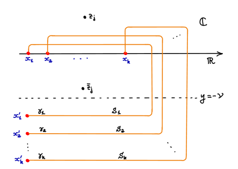
Figure 1. The extended Lefschetz fibration $E^{\prime}$ and the matching spheres $S_{j}$, projected to $\mathbb{C}$.

Proof of Proposition 3.3.1.

Statements (1), (2) and (4) follow from the theory developed in [Sei2, Sections 15d, 16e].

To prove (3) we begin by showing that $\omega_{E^{\prime}}$ is exact. Denote $E^{+}:=E|_{\{-\nu<\text{Im}\,z\}}$. Let $\gamma^{\prime}_{i}\subset\mathbb{C}$ be the path obtained from $\gamma_{i}$ by chopping a little neighborhood of its second end near $x^{\prime}_{i}$, namely $\gamma^{\prime}_{i}=\gamma_{i}\setminus D^{\prime}_{i}$, where $D^{\prime}_{i}$ is a little open disk around $x^{\prime}_{i}$. Fix also another point $y_{i}\in\gamma_{i}\cap E^{+}$ which is different from $x_{i}$.

Denote by $T_{x^{\prime}_{i}}\subset E^{\prime}$ the Lefschetz thimble emanating from $p_{i}$ along the path $\gamma^{\prime}_{i}$ and by $T_{y_{i}}\subset T_{x^{\prime}_{i}}$ the part of that thimble lying over $\gamma^{\prime}_{i}$, between $x_{i}$ and $y_{i}$. Denote by $\partial T_{x^{\prime}_{i}}$ and $\partial T_{y_{i}}$ the boundaries of these “partial” thimbles. These are Lagrangian spheres in the fibers of $E^{\prime}$ over $x^{\prime}_{i}$ and $y_{i}$ respectively.

By standard topological arguments there is a canonical isomorphism

$$\kappa:H_{2}(E^{+},\cup_{i=1}^{k}\partial T_{y_{i}})\longrightarrow H_{2}(E^{\prime}),$$ (18)

where the homologies are taken with any given coefficient group. This isomorphism is induced from the following chain-level map. Let $C$ be a relative cycle of $(E^{+},\cup_{i=1}^{k}\partial T_{y_{i}})$. For $w\in\gamma_{i}$ denote by $\Pi_{\gamma_{i}}^{y_{i},w}$ the parallel transport (with respect to the connection induced by $\omega_{E^{\prime}}$) along $\gamma_{i}$ from $E^{\prime}_{y_{i}}=E_{y_{i}}$ to $E^{\prime}_{w}$. Take the part of $\partial C$ lying in $\partial T_{y_{i}}$ and consider its trail under this parallel transport from $y_{i}$ till $x^{\prime}_{i}$, namely the union of $\Pi_{\gamma_{i}}^{y_{i},w}(\partial C\cap\partial T_{y_{i}})$, where $w$ runs along $\gamma_{i}$ between $y_{i}$ and $x^{\prime}_{i}$. Note that while $\Pi_{\gamma_{i}}^{y_{i},w}$ is in general not defined for the end point $w=x^{\prime}_{i}$, here we apply $\Pi_{\gamma_{i}}^{y_{i},x^{\prime}_{i}}$ to $\partial C\cap\partial T_{y_{i}}$ which yields the point $p^{\prime}_{i}$. Therefore the trail of $\partial C\cap\partial T_{y_{i}}$ along $\gamma_{i}$ between $y_{i}$ and $x^{\prime}_{i}$ is well defined and gives another relative cycle in $(E^{\prime},\partial T_{y_{i}})$, which we denote by $\text{Tr}_{y_{i},x^{\prime}_{i}}(\partial C)$. Note that $\partial\text{Tr}_{y_{i},x^{\prime}_{i}}(\partial C)=-(\partial C\cap\partial T_{y_{i}})$.

We can now cap the trails $\text{Tr}_{y_{i},x^{\prime}_{i}}(\partial C)$, $i=1,\ldots,k$, to $C$ along $\partial C\cap\partial T_{y_{i}}$, and obtain at the end an absolute cycle $C^{\prime}$ in $E^{\prime}$. The map $\kappa$ is induced by the chain level map $C\longmapsto C^{\prime}$.

In order to show that $\omega_{E^{\prime}}$ is exact, we will use the isomorphism $\kappa$, with coefficients in $\mathbb{R}$. It is enough to prove that $\langle[\omega_{E^{\prime}}],\kappa(A)\rangle=0$ for every $A\in H_{2}(E^{+},\cup_{i=1}^{k}\partial T_{y_{i}};\mathbb{R})$. For this end, note that $\omega_{E^{\prime}}$ vanishes over each of the trails $\text{Tr}_{y_{i},x^{\prime}_{i}}(\partial C)$, hence

$$\langle[\omega_{E^{\prime}}],\kappa(A)\rangle=\langle[\omega_{E^{\prime}}],A\rangle=\langle[\omega_{E}],A\rangle,$$

where the last equality holds because $\omega_{E^{\prime}}|_{E^{+}}=\omega_{E}|_{E^{+}}$. Now $\omega_{E}=d\lambda_{E}$, hence

$$\langle[\omega_{E}],A\rangle=\sum_{i=1}^{k}\langle[\lambda_{E}|_{\partial T_{y_{i}}}],\partial_{i}A\rangle,$$ (19)

where $\partial_{i}A$ is the component of $\partial A$ corresponding to $H_{1}(\partial T_{y_{i}};\mathbb{R})$. But $T_{y_{i}}$ is clearly a $\lambda_{E}$-exact Lagrangian submanifold, thus the right-hand side of (19) vanishes. This completes the proof that $\omega_{E^{\prime}}$ is exact.

Next, we prove that $\omega_{E^{\prime}}$ admits a primitive $\lambda_{E^{\prime}}$ that extends $\lambda_{E}|_{E^{+}}$. We claim that this would follow from the assertion that the map induced by inclusion $i_{*}:H_{1}(E^{+};\mathbb{R})\longrightarrow H_{1}(E^{\prime};\mathbb{R})$ is injective. Indeed, fix a small $\epsilon>0$ such that $\text{Im}\,x^{\prime}_{j}<-(\nu+\epsilon)$ for all $j$, and write $E^{+}_{\epsilon}=E|_{-(\nu+\epsilon)<\text{Im}\,z}$. Denote by $i^{\epsilon}:E^{+}_{\epsilon}\longrightarrow E^{\prime}$ the inclusion. Clearly $i_{*}$ is injective iff $i^{\epsilon}_{*}:H_{1}(E^{+}_{\epsilon};\mathbb{R})\longrightarrow H_{1}(E^{\prime})$ is injective. Fix any primitive $\lambda^{\prime}$ of $\omega_{E^{\prime}}$ and consider the $1$-form $\lambda_{E}|_{E^{+}}-\lambda^{\prime}|_{E^{+}}$. This form is closed because $\omega_{E}|_{E^{+}}=\omega_{E^{\prime}}|_{E^{+}}$. Since $i^{\epsilon}_{*}$ is injective, the restriction map $(i^{\epsilon})^{*}:H^{1}(E^{\prime};\mathbb{R})\longrightarrow H^{1}(E_{\epsilon}^{+};\mathbb{R})$ is surjective, hence there exists a closed $1$-form $\alpha^{\prime}$ on $E^{\prime}$ and a smooth function $f:E_{\epsilon}^{+}\longrightarrow\mathbb{R}$ such that $\alpha^{\prime}|_{E_{\epsilon}^{+}}=\lambda_{E}|_{E_{\epsilon}^{+}}-\lambda^{\prime}|_{E_{\epsilon}^{+}}+df$. Now cut off the function $f$ in between $E^{+}$ and $E^{+}_{\epsilon}$ to obtain another function $f^{\prime}:E^{\prime}\longrightarrow\mathbb{R}$ which coincides with $f$ on $E^{+}$ and vanishes outside of $E^{+}_{\epsilon}$. The desired $1$-form $\lambda_{E^{\prime}}$ is then given by

$$\lambda_{E^{\prime}}:=\alpha^{\prime}+\lambda^{\prime}-df^{\prime}.$$

To complete the proof it remains to show that

$$i_{*}:H_{1}(E^{+};\mathbb{R})\longrightarrow H_{1}(E^{\prime};\mathbb{R})$$ (20)

is injective. To this end, denote by $F=\pi^{-1}(w)$ the fiber of $\pi:E\longrightarrow\mathbb{R}$ over a regular value $w$ of $\pi$ with $w\in\{z\in\mathbb{C}\mid\text{Im}\,z>-\nu\}$.

Assume first that $\dim F>0$. By standard arguments, the inclusions $F\subset E^{+}$ and $F\subset E^{\prime}$ induce isomorphisms $H_{1}(F)\cong H_{1}(E^{+})$ and $H_{1}(F)\cong H_{1}(E^{\prime})$, where the homologies are taken with arbitrary coefficients. Therefore $i_{*}:H_{1}(E^{+})\longrightarrow H_{1}(E^{\prime})$ is an isomorphism.

Assume now that $\dim F=0$. Choose a small $\epsilon>0$ such that all the critical values of $\pi$ are in $\{\text{Im}\,z>-\nu+\epsilon\}$ and write $E^{\prime-}=E^{\prime}|_{\text{Im}\,z<-\nu+\epsilon}$. Note that $E^{+}\cap E^{\prime-}$ is homotopy equivalent to $F$ which is discrete, hence $H_{1}(E^{+}\cap E^{\prime-};\mathbb{R})=0$. By the Mayer-Vietoris sequence for $E^{\prime}=E^{+}\cup E^{\prime-}$ it follows that $i_{*}:H_{1}(E^{+};\mathbb{R})\longrightarrow H_{1}(E^{\prime};\mathbb{R})$ is injective.

This completes the proof of the injectivity of $i_{*}$ in (20) for all possible values of $\dim F$, hence also the proof of point (3) of the proposition.

Point (5) is obvious if $\dim F>0$ (since in that case $\dim(S_{i})\geq 2$). Assume that $\dim F=0$. In this case $N\approx S^{1}$, and without loss of generality we may assume that the number of real critical values of $\pi$ is $k=2$. (This is not really essential for the rest of the proof, it just simplifies a bit the notation.) Let $\lambda_{E^{\prime}}$ be a $1$-form from point (3), whose existence we have just proved. In the course of the argument below we will need to alter this $1$-form, so we will denote it by $\lambda^{\prime}$.

Let $E^{+}_{\epsilon}$ be as earlier in the proof. Denote by $j_{*}^{\epsilon}:H_{1}(E^{+}_{\epsilon};\mathbb{R})\longrightarrow H_{1}(E,\partial T_{x^{\prime}_{1}}\cup\partial T_{x^{\prime}_{2}};\mathbb{R})$, $i_{*}^{\epsilon}:H_{1}(E^{+}_{\epsilon};\mathbb{R})\longrightarrow H_{1}(E^{\prime};\mathbb{R})$ the maps induced by the inclusion $E^{+}_{\epsilon}\subset E^{\prime}$. Similarly to the isomorphism from (18) we have also an isomorphism

$$\kappa:H_{1}(E,\partial T_{x^{\prime}_{1}}\cup\partial T_{x^{\prime}_{2}};\mathbb{R})\longrightarrow H_{1}(E^{\prime};\mathbb{R})$$

which we continue denoting by $\kappa$ and which is defined by exactly the same means.

Consider the homology classes $[S_{1}],[S_{2}]\in H_{1}(E^{\prime};\mathbb{R})$ as well as the subspace $\textnormal{image\,}i^{\epsilon}_{*}\subset H_{1}(E^{\prime};\mathbb{R})$. We claim that no non-trivial linear combination of $[S_{1}],[S_{2}]$ belongs to $\textnormal{image\,}i^{\epsilon}_{*}$. This can be easily seen by looking at the images of $\kappa^{-1}[S_{1}]=[T_{x^{\prime}_{1}}]$, $\kappa^{-1}[S_{2}]=[T_{x^{\prime}_{2}}]$ under the the connecting homomorphism

$$\partial_{*}:H_{1}(E,\partial T_{x^{\prime}_{1}}\cup\partial T_{x^{\prime}_{2}};\mathbb{R})\longrightarrow H_{0}(\partial T_{x^{\prime}_{1}}\cup\partial T_{x^{\prime}_{2}};\mathbb{R})=H_{0}(\partial T_{x^{\prime}_{1}};\mathbb{R})\oplus H_{0}(\partial T_{x^{\prime}_{2}};\mathbb{R})$$

and noting that $\kappa^{-1}(\textnormal{image\,}i^{\epsilon}_{*})=\textnormal{image\,}j^{\epsilon}_{*}$ is sent to $0$ by $\partial_{*}$.

In view of the preceding claim we can find a closed $1$-form $\theta$ on $E^{\prime}$ such that:

1. $[\theta]\in H^{1}(E^{\prime};\mathbb{R})$ vanishes on $\textnormal{image\,}i^{\epsilon}_{*}$.

2. $\langle[\theta],[S_{1}]\rangle=\int_{S_{1}}\lambda^{\prime}$ and $\langle[\theta],[S_{2}]\rangle=\int_{S_{2}}\lambda^{\prime}$.

By the property of $\theta$ we have $(i^{\epsilon})^{*}[\theta]=0\in H^{1}(E^{+}_{\epsilon};\mathbb{R})$, hence there exists a smooth function $h:E^{+}_{\epsilon}\longrightarrow\mathbb{R}$ such that $\theta|_{E^{+}_{\epsilon}}=dh$. Now, cutoff $h$ near $\{\text{Im}\,z=-\nu-\epsilon\}$ and extend the resulting function to a smooth function $h^{\prime}:E^{\prime}\longrightarrow\mathbb{R}$ which vanishes on $\{\text{Im}\,z\leq-\nu-\epsilon\}$ and such that $h^{\prime}=h$ on $E^{+}=\{\text{Im}z>-\nu\}$. Replacing the form $\lambda_{E^{\prime}}$ provided by point (3) of the proposition by the form

$$\lambda^{\prime\prime}:=\lambda^{\prime}-\theta+dh^{\prime}$$

we still obtain a primitive of $\omega_{E^{\prime}}$ that coincides with $\lambda_{E}$ over $E^{+}$ and such that the matching spheres $S_{1}$, $S_{2}$ are $\lambda^{\prime\prime}$-exact. This completes the proof of point (5) of the proposition in case the fibers of $\pi:E\longrightarrow\mathbb{C}$ are $0$-dimensional. ∎

4. Floer theory in $E$ versus $E^{\prime}$

Recall that the extended Lefschetz fibration $\pi^{\prime}:E^{\prime}\longrightarrow\mathbb{C}$ from §3.3 has been constructed such that it coincides, together with its associated structures, with the original Lefschetz fibration $\pi:E\longrightarrow\mathbb{C}$ over $\{z\in\mathbb{C}\mid-\nu<\text{Im}z\}$.

Let $L_{0},L_{1}\subset E^{\prime}$ be two marked exact Lagrangians and assume that $L_{0},L_{1}\subset E^{\prime}|_{\{-\nu<\text{Im}z\}}=E|_{\{-\nu<\text{Im}z\}}$. By the arguments from [BC4] the Floer complexes of $(L_{0},L_{1})$ coincide, when viewed in $E$ and in $E^{\prime}$, provided we choose the right Floer data. More precisely, let $H$ be a Hamiltonian function compactly supported in $E|_{\{-\nu<\text{Im}z\}}$. Then there exist regular Floer data $\mathscr{D}=(H,J)$ in $E$ and $\mathscr{D}^{\prime}=(H,J^{\prime})$ in $E^{\prime}$, with the same Hamiltonian function $H$ such that all the Floer trajectories for $(L_{0},L_{1})$ with respect to $\mathscr{D}$ coincide with those for $\mathscr{D}^{\prime}$ and they all lie inside $E|_{\{-\nu<\text{Im}z\}}$. This easily follows from the open mapping theorem for holomorphic functions, by choosing appropriate compatible almost complex structures $J$ and $J^{\prime}$ for which the projections $\pi$ and $\pi^{\prime}$ are holomorphic. Consequently we have a chain isomorphism (induced by the identity map on $\mathcal{O}(H)$)

$$CF(L_{0},L_{1};\mathscr{D};E)\longrightarrow CF(L_{0},L_{1};\mathscr{D}^{\prime};E^{\prime})$$ (21)

which preserves the action filtration. The $E$ and $E^{\prime}$ in the notation of the Floer complexes in the preceding formula indicate the ambient manifold in which the respective Floer complex is being considered. Consequently (21) induces an action preserving isomorphism of persistence modules

$$HF^{\leq\bullet}(L_{0},L_{1};E)\cong HF^{\leq\bullet}(L_{0},L_{1};E^{\prime}),$$

hence the spectral invariants and boundary depths of $CF(L_{0},L_{1})$, viewed either in $E$ or in $E^{\prime}$, coincide.

The above can be generalized to the Fukaya categories of $E$ and $E^{\prime}$. More specifically, denote by $\mathcal{F}uk(E)$ and $\mathcal{F}uk(E^{\prime})$ the Fukaya categories of $E$ and $E^{\prime}$, whose objects are the closed marked exact Lagrangian submanifolds in $E$ and $E^{\prime}$. Let $\mathcal{F}uk(E;-\nu)\subset\mathcal{F}uk(E)$ be the full subcategory whose objects are closed exact Lagrangians $L\subset E|_{\{-\nu<\text{Im}z\}}$. As explained in [BC4] it is possible to choose the auxiliary data required for the definitions of $\mathcal{F}uk(E)$ and $\mathcal{F}uk(E^{\prime})$ in such a way that the inclusion of objects $\textnormal{Ob}(\mathcal{F}uk(E;-\nu))\subset\textnormal{Ob}(\mathcal{F}uk(E^{\prime}))$ extends to a (homologically) full and faithful $A_{\infty}$-functor $\text{Inc}:\mathcal{F}uk(E;-\nu)\longrightarrow\mathcal{F}uk(E^{\prime})$. Moreover, if we view $\mathcal{F}uk(E;-\nu)$ and $\mathcal{F}uk(E^{\prime})$ as weakly filtered $A_{\infty}$-categories, we can assume that the functor Inc is a weakly filtered functor (see §2.3 and §7.5 for a brief explanation of these concepts, and [BCS, §2] for the precise definitions and more details).

This has the following consequence for $A_{\infty}$-modules. Let $L\subset E^{\prime}$ be a marked exact Lagrangian and assume that $L\subset E|_{\{-\nu<\text{Im}z\}}$. Denote by $\mathscr{L}^{E^{\prime}}$ the Yoneda module of $L$, viewed as an $A_{\infty}$-module over $\mathcal{F}uk(E^{\prime})$ and by $\mathscr{L}^{E,-\nu}$ the Yoneda module of $L$ over $\mathcal{F}uk(E;-\nu)$. Both modules are weakly filtered in the sense of [BCS] and with the right choices of auxiliary data for $\mathcal{F}uk(E;-\nu)$, $\mathcal{F}uk(E^{\prime})$ we have that

$$\text{Inc}^{*}(\mathscr{L}^{E^{\prime}})=\mathscr{L}^{E,-\nu}$$

as weakly filtered $\mathcal{F}uk(E;-\nu)$-modules.

Next, we compare the Floer theory of the matching spheres $S_{j}$ in $E^{\prime}$ with the Floer theory of the thimbles $T^{{}^{\uparrow}}_{x_{j}}$ in $E$, defined on page 3.1. Fix a rectangle $\mathcal{R}\subset\mathbb{C}$ of the type

$$\mathcal{R}=\{x+iy\in\mathbb{C}\mid x\in(a,b),-\nu<y<\epsilon\}$$ (22)

such that $S_{j}\cap\pi^{\prime-1}(\mathcal{R})=T^{{}^{\uparrow}}_{x_{j}}\cap\pi^{-1}(\mathcal{R})$. (See Figure 2.)

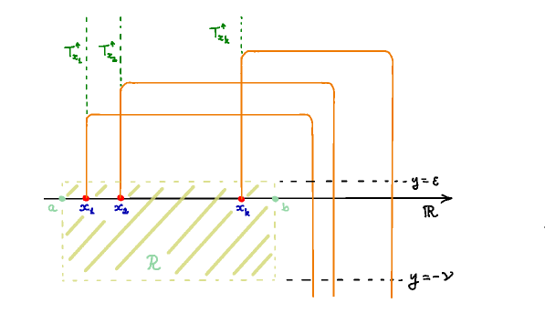
Figure 2. The rectangle $\mathcal{R}$ and the projection to $\mathbb{C}$ of the thimbles $T^{{}^{\uparrow}}_{x_{j}}$.

Let $L\subset E^{\prime}$ be a marked exact Lagrangian and assume that $\pi^{\prime}(L)\subset\mathcal{R}$. Let $H$ be a Hamiltonian function compactly supported in $\pi^{-1}(\mathcal{R})$. Then there exist almost complex structures $J$ on $E$ and $J^{\prime}$ on $E^{\prime}$, compatible with $\omega_{E}$ and $\omega_{E^{\prime}}$ respectively, making the Floer data $\mathscr{D}=(H,J)$ and $\mathscr{D}^{\prime}=(H,J^{\prime})$ regular and such that the Floer trajectories for $(L,S_{j};\mathscr{D}^{\prime})$ in $E^{\prime}$ and the Floer trajectories of $(L,T^{{}^{\uparrow}}_{x_{j}};\mathscr{D})$ in $E$ coincide and moreover all these trajectories lie inside $\pi^{-1}(\mathcal{R})$. This follows again from an open mapping theorem argument as in [BC4].

It follows that the identity map on $\mathcal{O}(H)$ gives an action preserving chain isomorphism

$$CF(L,S_{j};\mathscr{D}^{\prime};E^{\prime})\longrightarrow CF(L,T^{{}^{\uparrow}}_{x_{j}};\mathscr{D};E).$$

Here we view $T^{{}^{\uparrow}}_{x_{j}}\subset E$ as a marked exact Lagrangian with primitive function adjusted such that it coincides with the given primitive function of $S_{j}$ along $S_{j}\cap\pi^{\prime-1}(\mathcal{R})=T^{{}^{\uparrow}}_{x_{j}}\cap\pi^{-1}(\mathcal{R})$.

Denote by $\mathcal{F}uk(E;\mathcal{R})\subset\mathcal{F}uk(E^{\prime})$ the full subcategory whose objects are marked exact Lagrangians $L$ with $\pi(L)\subset\mathcal{R}$. Similarly to Inc we have weakly filtered inclusion $A_{\infty}$-functors $\text{Inc}_{\mathcal{R},-\nu}:\mathcal{F}uk(E;\mathcal{R})\longrightarrow\mathcal{F}uk(E;-\nu)$ and $\text{Inc}_{\mathcal{R},E^{\prime}}:\mathcal{F}uk(E;\mathcal{R})\longrightarrow\mathcal{F}uk(E^{\prime})$ with $\text{Inc}_{\mathcal{R},E^{\prime}}=\text{Inc}\circ\text{Inc}_{\mathcal{R},-\nu}$.

Putting all these constructions together we deduce:

Lemma 4.0.1.

Let $\mathcal{S}_{j}$ be the Yoneda module of $S_{j}$ and let $\mathcal{T}^{{}^{\uparrow}}_{x_{j}}$ be the Yoneda module of $T^{{}^{\uparrow}}_{x_{j}}$, the latter being viewed as a module over $\mathcal{F}uk(E;-\nu)$. With the appropriate choice of auxiliary data, we have

$$\text{Inc}_{\mathcal{R},E^{\prime}}^{*}(\mathcal{S}_{j})=\text{Inc}_{\mathcal{R},-\nu}^{*}(\mathcal{T}^{{}^{\uparrow}}_{x_{j}})$$ (23)

as weakly filtered $\mathcal{F}uk(E;\mathcal{R})$-modules.

5. Cone decompositions in Lefschetz fibrations

Recall from [BC4] that the Yoneda modules associated to closed Lagrangian submanifolds (or more generally Lagrangian cobordisms), satisfying appropriate exactness or monotonicity conditions, in a Lefschetz fibration $E$ can be represented as iterated cones of modules involving the matching spheres $S_{j}$ in the extended Lefschetz fibration $E^{\prime}$. We will apply these results below, to the fibrations $E$ and $E^{\prime}$ constructed in §3.1 - §3.3 above, while also keeping track of the action filtrations.

Let $\pi:E\longrightarrow\mathbb{R}$ be a real Lefschetz fibration with critical values $x_{1},\ldots,x_{k},z_{1},\macc@depth\char 1\relax\frozen@everymath{\macc@group}\macc@set@skewchar\macc@nested@a 111{z}_{1},\ldots,z_{l},\macc@depth\char 1\relax\frozen@everymath{\macc@group}\macc@set@skewchar\macc@nested@a 111{z}_{l}$ and let $\pi^{\prime}:E^{\prime}\longrightarrow\mathbb{C}$ be the extended Lefschetz fibration, as in §3.3. Fix $\epsilon>0$ with $\epsilon<|\text{Im}\,z_{j}|$ for every $j$. Let $K\subset E$ be a closed $\lambda_{E}$-exact Lagrangian submanifold and assume that $K\subset E|_{\{|\text{Im}|\,z<\epsilon\}}$. Consider the matching spheres $S_{j}\subset E^{\prime}$ and denote by $\tau_{S_{j}}:E^{\prime}\longrightarrow E^{\prime}$ the Dehn-twist around $S_{j}$, supported in a small neighborhood of $S_{j}$. Note that $\tau_{S_{j}}$ is well defined up to Hamiltonian isotopy (supported near $S_{j}$) since the sphere $S_{j}$, being a matching sphere, has a canonical smooth identification with $S^{n}$ ($2n=\dim_{\mathbb{R}}E$) up to smooth isotopy.

Put $K^{(0)}:=K$, $K^{(j)}:=\tau_{S_{j}}(K^{(j-1)})$, $j=1,\ldots,k$. We view these Lagrangians as objects of the $\lambda_{E^{\prime}}$-exact Fukaya category $\mathcal{F}uk(E^{\prime})$ of $E^{\prime}$. Denote by $\mathcal{K}^{(j)}$ the Yoneda modules associated to $K^{(j)}$, $j=0,\ldots,k$. Write also $\mathcal{K}:=\mathcal{K}^{(0)}$ for the Yoneda module of $K$ and denote by $\mathcal{S}_{j}$, $j=1,\ldots,k$, the Yoneda modules associated to the matching spheres $S_{j}$.

By the results of [BC4], $\mathcal{K}$ is quasi-isomorphic, in the $A_{\infty}$-category of modules over $\mathcal{F}uk(E^{\prime})$, to the following iterated cone of $\mathcal{F}uk(E^{\prime})$-modules:

$$\mathcal{K}\cong[\mathcal{B}_{1}\longrightarrow\cdots\longrightarrow\mathcal{B}_{k}\longrightarrow\mathcal{K}^{(k)}],$$ (24)

where each of the modules $\mathcal{B}_{j}$, $j=1,\ldots,k$, has itself an iterated cone decomposition of the following type:

$$\mathcal{B}_{j}=[\mathcal{S}_{j}\otimes CF(S_{j},K)\longrightarrow\mathcal{B}_{j,1}\longrightarrow\mathcal{B}_{j,2}\longrightarrow\cdots\longrightarrow\mathcal{B}_{j,j-1}].$$ (25)

In order to describe the modules $\mathcal{B}_{j,d}$, $1\leq d\leq j-1$, that appear in (25) we need a bit of notation. Denote by $\mathcal{I}_{d,j-1}$ the set of all multi-indices $\underline{i}=(i_{1},\ldots,i_{d})$ with $1\leq i_{1}<i_{2}<\cdots<i_{d}\leq j-1$. We order the elements of $\mathcal{I}_{d,j-1}$ by the lexicographic order. For each multi-index $\underline{i}\in\mathcal{I}_{d,j-1}$ put

$$\mathcal{C}_{\underline{i},j}:=\mathcal{S}_{j}\otimes CF(S_{j},S_{i_{d}})\otimes CF(S_{i_{d}},S_{i_{d-1}})\otimes\cdots\otimes CF(S_{i_{2}},S_{i_{1}})\otimes CF(S_{i_{1}},K).$$ (26)

Let $m_{d,j-1}:=\#\mathcal{I}_{d,j-1}$ and order the elements of $\mathcal{I}_{d,j-1}=\{\underline{i}^{(1)},\ldots,\underline{i}^{(m_{d,j-1})}\}$ in such a way that $\underline{i}^{(1)}\precneqq\underline{i}^{(2)}\precneqq\cdots\precneqq\underline{i}^{(m_{d,j-1})}$. Then

$$\mathcal{B}_{j,d}=[\mathcal{C}_{\underline{i}^{(1)},j}\longrightarrow\mathcal{C}_{\underline{i}^{(2)},j}\longrightarrow\cdots\longrightarrow\mathcal{C}_{\underline{i}^{(m_{d,j-1})},j}].$$ (27)

Having established a cone decomposition of the module $\mathcal{K}$ over the $A_{\infty}$-category $\mathcal{F}uk(E^{\prime})$ we consider its pull-back to Fukaya categories associated to $E$. Recall from §4 that we have the Fukaya categories $\mathcal{F}uk(E;\mathcal{R})$ and $\mathcal{F}uk(E;-\nu)$. We take the rectangle $\mathcal{R}$ from (22) to be wide enough such that it contains $\pi(K)$. Recall also the inclusion functor

$$\text{Inc}_{\mathcal{R},E^{\prime}}:\mathcal{F}uk(E;\mathcal{R})\longrightarrow\mathcal{F}uk(E^{\prime})$$

that factors as the composition $\text{Inc}_{\mathcal{R},E^{\prime}}=\text{Inc}\,\circ\,\text{Inc}_{\mathcal{R},-\nu}$ of the two functors

$$\text{Inc}_{\mathcal{R},-\nu}:\mathcal{F}uk(E;\mathcal{R})\longrightarrow\mathcal{F}uk(E;-\nu),\quad\text{Inc}:\mathcal{F}uk(E;-\nu)\longrightarrow\mathcal{F}uk(E^{\prime}).$$

By pulling back the cone decomposition (24) via $\text{Inc}_{\mathcal{R},E^{\prime}}^{*}$ we obtain a similar cone decomposition for $\mathcal{K}$ (now viewed as a module over $\mathcal{F}uk(E;\mathcal{R})$), where the modules $\mathcal{S}_{j}$ in (25) and (26) are replaced by $\text{Inc}^{*}_{\mathcal{R},-\nu}(\mathcal{T}^{{}^{\uparrow}}_{x_{j}})$, see (23). (Note that the terms involving the Floer complexes of $S_{j}$ and and of $S_{i_{l}}$ remain unchanged.)

Finally, we claim that the pullback $\text{Inc}_{\mathcal{R},E^{\prime}}^{*}\mathcal{K}^{(k)}$ of the the module $\mathcal{K}^{(k)}$ which appears last in (24) is acyclic.

We will outline below in §5.1 the proof of the cone decomposition (24), the expressions (25) - (27) as well as the acyclicity of $\text{Inc}_{\mathcal{R},E^{\prime}}^{*}\mathcal{K}^{(k)}$. Then in §5.2 and §5.3 we will refine these results to take into account also the action filtrations.

Before we turn to these details, here is a concrete example showing how the cone decomposition of $\mathcal{K}$ looks like in case the number of real critical values of $\pi$ is $k=3$:

$$\mathcal{K}\cong[ \mathcal{S}_{1}\otimes CF(S_{1},K)\longrightarrow$$

$$\mathcal{S}_{2}\otimes CF(S_{2},K)\longrightarrow\mathcal{S}_{2}\otimes CF(S_{2},S_{1})\otimes CF(S_{1},K)\longrightarrow$$

$$\mathcal{S}_{3}\otimes CF(S_{3},K)\longrightarrow\mathcal{S}_{3}\otimes CF(S_{3},S_{2})\otimes CF(S_{1},K)\longrightarrow\mathcal{S}_{3}\otimes CF(S_{3},S_{2})\otimes CF(S_{2},K)\longrightarrow$$

$$\mathcal{S}_{3}\otimes CF(S_{3},S_{2})\otimes CF(S_{2},S_{1})\otimes CF(S_{1},K)\longrightarrow\mathcal{K}^{(3)}]$$

5.1. Exact triangles associated to Dehn twists

Let $(X^{2n},\omega=d\lambda)$ be a Liouville domain and $S^{n}\xrightarrow{\;\approx\;}S\subset X$ a parametrized Lagrangian sphere. In case $n=1$ we additionally assume that $S$ is $\lambda$-exact. Let $\tau:=\tau_{S}:X\longrightarrow X$ be a symplectomorphism, supported in $\textnormal{Int\,}X$, which represents the symplectic mapping class of the Dehn twist around $S$. Note that $\tau$ is an exact symplectomorphism, hence sends exact Lagrangians to exact Lagrangians.

A well known result of Seidel [Sei1, Sei2] says that for every exact Lagrangian $Q\subset X$ there is the following distinguished triangle in the derived Fukaya category $\mathcal{F}uk(X)$:

(28)

Here $\mathcal{S}$, $\mathcal{Q}$ and $\tau(\mathcal{Q})$ stand for the $A_{\infty}$-modules corresponding to $S$, $Q$ and $\tau(Q)$ under the Yoneda embedding.

The above distinguished triangle implies that, up to a quasi-isomorphism of modules, $\mathcal{Q}$ can be expressed as the following mapping cone:

$$\mathcal{Q}\cong[\mathcal{S}\otimes CF(S,Q)\longrightarrow\tau(\mathcal{Q})].$$ (29)

By rotating (28) we obtain also the following quasi-isomorphism:

$$\tau(\mathcal{Q})\cong[\mathcal{Q}\longrightarrow\mathcal{S}\otimes CF(S,Q)].$$ (30)

Note that here and in what follows we work in an ungraded setting, hence no grading shifts appear in any of (28) - (30).

We now turn to the cone decomposition (24), and assume that $(X,d\lambda)=(E^{\prime},\lambda_{E^{\prime}})$ as in §3.3. The decomposition (24) follows by successively applying (29) and (30). Specifically, we begin with $\mathcal{K}^{(1)}=\tau_{S_{1}}(\mathcal{K})$ and obtain from (29):

$$\mathcal{K}\cong[\mathcal{S}_{1}\otimes CF(S_{1},K)\longrightarrow\mathcal{K}^{(1)}].$$ (31)

By the same argument we also have $\mathcal{K}^{(1)}\cong[\mathcal{S}_{2}\otimes CF(S_{1},K^{(1)})\longrightarrow\mathcal{K}^{(2)}]$, which together with (31) gives:

$$\mathcal{K}\cong[\mathcal{S}_{1}\otimes CF(S_{1},K)\longrightarrow\mathcal{S}_{2}\otimes CF(S_{2},K^{(1)})\longrightarrow\mathcal{K}^{(2)}].$$ (32)

But by (30) we have $\mathcal{K}^{(1)}\cong[\mathcal{K}\longrightarrow\mathcal{S}_{1}\otimes CF(S_{1},K)]$. Substituting this into (32) yields:

$$\mathcal{K}\cong[\mathcal{S}_{1}\otimes CF(S_{1},K)\longrightarrow\mathcal{S}_{2}\otimes CF(S_{2},K)\longrightarrow\mathcal{S}_{2}\otimes CF(S_{2},S_{1})\otimes CF(S_{1},K)\longrightarrow\mathcal{K}^{(2)}].$$ (33)

Continuing in a similar vein, decomposing $\mathcal{K}^{(2)}$, $\mathcal{K}^{(3)}$ etc.  we obtain the cone decomposition (24) with items as described in (25) - (27).

It remains to address the acyclicity of the module $\text{Inc}_{\mathcal{R},E^{\prime}}^{*}\mathcal{K}^{(k)}$. (Recall $K^{(k)}=\tau_{S_{k}}\cdots\tau_{S_{1}}(K)$). This follows from [BC4, §4.4], where it is proved that there is a Hamiltonian diffeomorphism $\phi:E^{\prime}\longrightarrow E^{\prime}$ such that $\phi(K^{(k)})\subset E^{\prime}|_{\{\text{Im}\,z\leq-\nu\}}$. (See also [BC2] for more details.) In particular, for every Lagrangian submanifold $L\subset\pi^{\prime-1}(\mathcal{R})$ we have $CF(L,\phi(K^{(k)}))=0$.

5.2. Taking filtrations into account

We now go back to the cone decomposition (24) and review it from the perspective of action filtrations.

From now on we assume all the exact Lagrangian submanifolds to be marked, unless otherwise stated. By a slight abuse of notation, we now redefine the objects of the Fukaya categories $\mathcal{F}uk(E)$, $\mathcal{F}uk(E^{\prime})$, as well as $\mathcal{F}uk(E;\mathcal{R})$, $\mathcal{F}uk(E;-\nu)$, to be marked exact Lagrangians, subject to the additional constraints in each of these categories. These categories now become weakly filtered $A_{\infty}$-categories, where the filtrations are induced by the action functional. We refer the reader to [BCS, §2] for the definitions and basic theory of weakly filtered $A_{\infty}$-categories and weakly filtered modules over such.

Below we will take the exact Lagrangian $K\subset E|_{\{|\text{Im}|\,z<\epsilon\}}$ to have an arbitrary marking. This marking induces a marking on $K^{(j)}=\tau_{S_{j}}\cdots\tau_{S_{1}}(K)$, $j=1,\ldots,k$, see §5.3, page 5.3. The Lagrangian spheres $S_{j}$ are also assumed to be marked in advance.

Note that all the items in the cone decomposition (24), as detailed in (25) - (27) are weakly filtered modules. This is so because the $\mathcal{S}_{j}$’s and $\mathcal{K}^{(k)}$ are Yoneda modules over a weakly filtered $A_{\infty}$-category, and the chain complexes $CF(S_{i_{l}},S_{i_{l-1}})$ and $CF(S_{j},K)$ are filtered.

Next, we claim that all the maps in the iterated cones (24), (25) and (27) are weakly filtered maps. This means, in particular, that when evaluating these iterated cones modules on a given exact Lagrangian $L$, each of these maps specializes to a filtered chain map that shifts filtrations by an amount bounded from above uniformly in $L$. More specifically:

Proposition 5.2.1.

In the iterated cone (27)

$$\mathcal{B}_{j,d}=[\mathcal{C}_{\underline{i}^{(1)},j}\xrightarrow{\;\varphi_{1,j}\;}[\mathcal{C}_{\underline{i}^{(2)},j}\xrightarrow{\;\varphi_{2,j}\;}[\cdots\xrightarrow{\;\;\;\;}[\mathcal{C}_{\underline{i}^{(m_{d,j-1}-1)},j}\xrightarrow{\;\varphi_{m_{d,j-1}-1,j}\;}\mathcal{C}_{\underline{i}^{(m_{d,j-1})},j}]\cdots]]],$$ (34)

each of the module homomorphisms $\varphi_{l,j}$ is weakly filtered, and shifts action by $\leq s_{\varphi_{l,j}}$, for some $s_{\varphi_{l,j}}\geq 0$.

This implies that the right-hand side of (34) is filtered using the filtrations of the factors $\mathcal{C}_{\underline{i}^{(l)},j}$ and the recipe (53).

In particular, for every exact Lagrangian $L$, the module homomorphism $\varphi_{l,j}$ specializes to an $s_{\varphi_{l,j}}$-filtered chain map (still denoted by $\varphi_{l,j}$):

$$\varphi_{l,j}:\mathcal{C}_{\underline{i}^{(l)},j}(L)\longrightarrow[\mathcal{C}_{\underline{i}^{(l+1)},j}(L)\xrightarrow{\;\varphi_{l+1,j}\;}[\cdots\xrightarrow{\;\;\;\;}[\mathcal{C}_{\underline{i}^{(m_{d,j-1}-1)},j}(L)\xrightarrow{\;\varphi_{m_{d,j-1}-1,j}\;}\mathcal{C}_{\underline{i}^{(m_{d,j-1})},j}(L)]\cdots]].$$

A crucial point for us will be that the filtration-shifts $s_{\varphi_{l,j}}$ are independent of $L$.

Having filtered the modules $\mathcal{B}_{j,d}$, the preceding statements apply also to the maps in the iterated cone of (25), and finally also to the right-hand side of (24). We will prove Proposition 5.2.1 in §5.3 below.

Furthermore, we claim that the module quasi-isomorphism at (24) between $\mathcal{K}$ and the (now weakly filtered) iterated cone on the right-hand side is filtered in the following sense.

Proposition 5.2.2.

There exist $s_{\mathcal{K}}\geq 0$ and weakly-filtered module homomorphisms

$$\varphi:\mathcal{K}\longrightarrow[\mathcal{B}_{1}\longrightarrow\cdots\longrightarrow\mathcal{B}_{k}\longrightarrow\mathcal{K}^{(k)}],\quad\psi:[\mathcal{B}_{1}\longrightarrow\cdots\longrightarrow\mathcal{B}_{k}\longrightarrow\mathcal{K}^{(k)}]\longrightarrow\mathcal{K}$$

that shift filtrations by $\leq s_{\mathcal{K}}$ and such that

$$\varphi\circ\psi=\textnormal{id}+\mu_{1}^{\text{mod}}(h^{\prime}),\quad\psi\circ\varphi=\textnormal{id}+\mu_{1}^{\text{(}mod)}(h^{\prime\prime})$$

for weakly filtered pre-module homomorphisms $h^{\prime},h^{\prime\prime}$ that shift filtrations by $\leq s_{\mathcal{K}}$.

The proof of this statement is again postponed to  §5.3. The constant $s_{\mathcal{K}}$ depends on $K$ (and its marking) as well as on the marking on the spheres $S_{1},\ldots,S_{k}$.

In particular, the above implies that for every exact Lagrangian $L$ we have chain maps

$$\varphi_{L}:CF(L,K)\longrightarrow[\mathcal{B}_{1}(L)\longrightarrow\cdots\longrightarrow\mathcal{B}_{k}(L)\longrightarrow CF(L,K^{(k)})],$$ (35)

$$\psi_{L}:[\mathcal{B}_{1}(L)\longrightarrow\cdots\longrightarrow\mathcal{B}_{k}(L)\longrightarrow CF(L,K^{(k)})]\longrightarrow CF(L,K),$$

which are $s_{\mathcal{K}}$-filtered and such that $\varphi_{L}\circ\psi_{L}$ and $\psi_{L}\circ\varphi_{L}$ are chain homotopic to the identities via chain homotopies that shift filtrations by $\leq s_{\mathcal{K}}$. Once again, it is important to stress that the bound on the action shift $s_{\mathcal{K}}$ is independent of $L$.

Phrased in the terminology of Definition 7.5.3, the above says that the module $\mathcal{K}$ (resp. filtered chain complex $CF(L,K)$) and the module on the right-hand side of (24) (resp. the filtered chain complex $[\mathcal{B}_{1}(L)\longrightarrow\cdots\longrightarrow\mathcal{B}_{k}(L)\longrightarrow CF(L,K^{(k)})]$) are at distance $\leq s_{\mathcal{K}}$ one from the other.

Finally, recall that the pullback module $\text{Inc}_{\mathcal{R},E^{\prime}}^{*}\mathcal{K}^{(k)}$ is acyclic. We claim that this acyclicity holds also in the filtered sense. Namely, there exists a constant $s_{C}=s_{C}(K)$, which depends on $K$, and a weakly filtered pre-module homomorphism $h:\text{Inc}_{\mathcal{R},E^{\prime}}^{*}\mathcal{K}^{(k)}\longrightarrow\text{Inc}_{\mathcal{R},E^{\prime}}^{*}\mathcal{K}^{(k)}$ that shifts action by $\leq s_{C}$ such that in $\hom_{\text{mod}_{\mathcal{F}uk(E;\mathcal{R})}}(\text{Inc}_{\mathcal{R},E^{\prime}}^{*}\mathcal{K}^{(k)},\text{Inc}_{\mathcal{R},E^{\prime}}^{*}\mathcal{K}^{(k)})$ we have $id=\mu_{1}^{\text{mod}}(h)$. In particular, for every exact Lagrangian $L\subset\pi^{-1}(\mathcal{R})$ we have:

$$\beta(CF(L,\mathcal{K}^{(k)}))\leq s_{C}.$$ (36)

Here, $\beta(CF(L,\mathcal{K}^{(k)}))$ is the boundary depth of the acyclic filtered chain complex $CF(L,\mathcal{K}^{(k)})$.

The inequality (36) follows from the last paragraph of §5.1 on page 5.1. Indeed, by standard Floer theory we can take $s_{C}=2\rho(\textnormal{id},\phi)$, where $\phi:E^{\prime}\longrightarrow E^{\prime}$ is a Hamiltonian diffeomorphism that sends $K^{(k)}$ to $E^{\prime}|_{\{\text{Im}\,z\leq-\nu\}}$, and $\rho$ stands for the Hofer metric on the group of Hamiltonian diffeomorphisms.

Remark 5.2.3.

The constant $s_{C}$ appearing in (36) depends apriori on $K$ (though not on $L$). A more careful argument, based on [BC4, §4.4], shows that the Hamiltonian diffeomorphisms $\phi$, mentioned above, can be taken to be at a uniformly bounded (in $K$) Hofer-distance from id, as long as we restrict to Lagrangians $K\subset E|_{\{|\text{Im}|\,z<\epsilon\}}$. Consequently the constant $s_{C}$ can be assumed to be independent of $K$.

However, this additional information will not be used in the rest of the paper. The reason is that we will use the filtered cone decomposition (24) only for one Lagrangian $K$, namely $K=N$ - the zero-section of $T^{*}(N)$ viewed as a Lagrangian in $E$.

5.3. Proof of the statements from §5.2

We continue to assume here all exact Lagrangian submanifolds (and cobordisms) to be marked.

We begin with a brief digression on inclusion and product functors. Let $(Y,d\lambda_{Y})$ be a Liouville manifold as in §2.2.2. Let $\gamma:\mathbb{R}\longrightarrow\mathbb{R}^{2}$ be a smooth proper embedding sending the ends of $\mathbb{R}$ to horizontal rays in $\mathbb{R}^{2}$. By abuse of notation we denote by $\gamma$ also the image of this embedding. By the results of [BC3, BCS] there is a weakly filtered $A_{\infty}$-functor (called in [BC3] “inclusion functor”) $\mathcal{I}_{\gamma}:\mathcal{F}uk(Y)\longrightarrow\mathcal{F}uk_{\text{cob}}(\mathbb{R}^{2}\times Y)$ which sends the object $L\subset Y$ to $\mathcal{I}_{\gamma}(L)=\gamma\times L\subset\mathbb{R}^{2}\times Y$. Here $\mathcal{F}uk(Y)$ stands for the Fukaya category of closed $\lambda_{Y}$-exact Lagrangians in $Y$ and $\mathcal{F}uk_{\text{cob}}(\mathbb{R}^{2}\times Y)$ for the Fukaya category of exact cobordisms in $\mathbb{R}^{2}\times Y$, with respect to the $1$-form $xdy\oplus\lambda_{Y}$.

Let $(X,\omega=d\lambda)$ be a Liouville manifold as in §2.2.2. We denote by $X^{-}$ the manifold $X$ endowed with the symplectic structure $-\omega$. Take $Y=X\times X^{-}$, endowed with the symplectic structure $\omega\oplus-\omega$ and Liouville form $\widetilde{\lambda}:=\lambda\oplus-\lambda$ (playing the role of $\lambda_{Y}$). Fix $\widetilde{\lambda}^{\prime}:=xdy\oplus\lambda\oplus-\lambda$ as the primitive of $\omega_{\mathbb{R}^{2}}\oplus\omega\oplus-\omega$.

Fix an exact Lagrangians $Q\subset X$. A slight variation on the inclusion functor $\mathcal{I}_{\gamma}$ is the $A_{\infty}$-functor $\mathcal{I}_{\gamma,Q}:\mathcal{F}uk(X)\longrightarrow\mathcal{F}uk_{\text{cob}}(\mathbb{R}^{2}\times X\times X^{-})$ which sends an exact Lagrangians $L\subset X$ to $\mathcal{I}_{\gamma,Q}(L):=\gamma\times L\times Q$. The construction of this functor is very similar to the construction of $\mathcal{I}_{\gamma}$ (for the case $Y=X\times X^{-}$), as detailed in [BC3]. In fact, $\mathcal{I}_{\gamma,Q}$ factors as $\mathcal{I}_{\gamma,Q}:=\mathcal{I}_{\gamma}\circ\mathcal{P}_{Q}$, where $\mathcal{P}_{Q}:\mathcal{F}uk(X)\longrightarrow\mathcal{F}uk(X\times X^{-})$ is the obvious functor that sends $L\subset X$ to $L\times Q\subset X\times X^{-}$.

The main ingredient to show Propositions 5.2.1 and 5.2.2 is to establish a filtered version of the Seidel’s Dehn-twist triangle (28) (or more precisely (29)). We pursue this now.

Lemma 5.3.1.

The mapping cone in equation (29) admits a filtered version.

In the course of the proof we will indicate more precisely the relevant shifts involved and their dependence on the choices involved in the construction.

Proof.

Let $(X^{2n},\omega=d\lambda)$ be a Liouville manifold as in §2.2.2 and $S\subset X$, $\tau=\tau_{S}:X\longrightarrow X$ be as at the beginning of §5.1. It is possible to choose $\tau$ (a representative of the Dehn-twist symplectic mapping class) such that $\tau$ is supported near $S$ and moreover such that $\tau^{*}\lambda=\lambda+dh_{\tau}$, where $h_{\tau}:X\longrightarrow\mathbb{R}$ is a smooth function compactly supported near $S$. (The latter easily follows from the fact that given any neighborhood of the zero-section in $T^{*}(S^{n})$, there is a model Dehn-twist $T^{*}(S^{n})\longrightarrow T^{*}(S^{n})$ supported in that neighborhood which is $\lambda_{\text{can}}$-exact, and the fact that the sphere $S$ is $\lambda$-exact.) Note that we have: $(\tau^{-1})^{*}\lambda=\lambda-d(h_{\tau}\circ\tau^{-1})$.

Let $Q\subset X$ be a marked exact Lagrangian with primitive $h_{Q}:Q\longrightarrow\mathbb{R}$ for $\lambda|_{Q}$. Then $\tau(Q)$ is also a marked exact Lagrangian. Indeed, $h_{\tau(Q)}:\tau(Q)\longrightarrow\mathbb{R}$ defined by

$$h_{\tau(Q)}(x):=h_{Q}(\tau^{-1}(x))+h_{\tau}(\tau^{-1}(x))$$

is a primitive of $\lambda|_{\tau(Q)}$. We will use this function to mark $\tau(Q)$.

We now get back to Dehn-twists, from the perspective of Lagrangian cobordism. By a result of Mak-Wu [MW] there exists an exact Lagrangian cobordism $W\subset\mathbb{R}^{2}\times X\times X^{-}$ with two negative ends and one positive end, as follows. The upper negative end is $S\times S$ and the lower negative end is the graph $\Gamma_{\tau^{-1}}$ of $\tau^{-1}$. The positive end is the graph of the identity map (i.e. the diagonal in $X\times X^{-}$). See Figure 3.

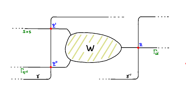
Figure 3. Projection to $\mathbb{R}^{2}$ of the Mak-Wu cobordism $W\subset\mathbb{R}^{2}\times X\times X^{-}$, and the curves $\gamma$, $\gamma^{\prime}$.

Let $\gamma\subset\mathbb{R}^{2}$ be the curve depicted in Figure 3, and denote by $\mathcal{W}$ the Yoneda module corresponding to $W\in\textnormal{Ob}(\mathcal{F}uk_{\text{cob}}(\mathbb{R}^{2}\times X\times X^{-})$. Denote also by $\mathcal{S}\times\mathcal{S}$, $\tau(\mathcal{Q})$ the Yoneda modules (over $\mathcal{F}uk(X\times X^{-})$ corresponding to the Lagrangians $S\times S$ and $\tau(\mathcal{K})$, respectively. Ignoring filtrations for the moment, a straightforward calculation (based on the theory from [BC3]) shows that the pullback module $\mathcal{I}_{\gamma,Q}^{*}\mathcal{W}$ coincides with a mapping cone

$$\mathcal{I}_{\gamma,Q}^{*}\mathcal{W}=[\mathcal{S}\otimes CF(S,Q)\xrightarrow{\;\varphi\;}\tau(\mathcal{Q})]$$ (37)

for some module homomorphism $\varphi:\mathcal{S}\otimes CF(S,Q)\longrightarrow\tau(\mathcal{Q})$.

Consider now the curve $\gamma^{\prime}\subset\mathbb{R}^{2}$ from Figure 3. Ignoring filtrations again, it is easy to see that $\mathcal{I}_{\gamma^{\prime},Q}^{*}\mathcal{W}=\mathcal{Q}$, the Yoneda module corresponding to $Q\subset X$.

The curves $\gamma$ and $\gamma^{\prime}$ are isotopic via a Hamiltonian isotopy which is horizontal at infinity. Therefore the modules $\mathcal{I}_{\gamma,Q}^{*}\mathcal{W}$ and $\mathcal{I}_{\gamma^{\prime},Q}^{*}\mathcal{W}$ are quasi-isomorphic (in the category $\text{mod}_{\mathcal{F}uk(X)}$). Thus we have a quasi-isomorphism

$$\mathcal{Q}\cong[\mathcal{S}\otimes CF(S,Q)\xrightarrow{\;\varphi\;}\tau(\mathcal{Q})].$$ (38)

Our goal now is to derive a coarse filtered version of (38). More specifically, we will have to address two thing: explain why the module homomorphism $\varphi$ is filtered, and then show that the quasi-isomorphism in (38) is weighted in the sense of Definition 7.5.3.

Note that $\widetilde{\lambda}^{\prime}$ coincides with $\widetilde{\lambda}$ along each horizontal end of $W$ (because $xdy$ vanishes along horizontal rays). We also have

$$\widetilde{\lambda}|_{\Gamma_{\textnormal{id}}}=0,\quad\widetilde{\lambda}|_{S\times S}=\lambda_{S}\oplus-\lambda_{S},\quad\widetilde{\lambda}|_{\Gamma_{\tau^{-1}}}=d(h_{\tau}\circ\tau^{-1}),$$

where $\lambda_{S}:=\lambda|_{S}$. Let $h_{W}:W\longrightarrow\mathbb{R}$ be a primitive of $\widetilde{\lambda}^{\prime}|_{W}$. By the above, $h_{W}$ restricts along each of the ends of $W$ to a primitive function for the restriction of $\widetilde{\lambda}$ to the Lagrangian corresponding to that end. We will use these functions, denoted by $h_{W,\Gamma_{\textnormal{id}}}$, $h_{W,S\times S}$ and $h_{W,\Gamma_{\tau^{-1}}}$, for primitives of $\widetilde{\lambda}|_{\Gamma_{\textnormal{id}}}$, $\widetilde{\lambda}|_{S\times S}$ and $\widetilde{\lambda}|_{\Gamma_{\tau^{-1}}}$ respectively. Note that $h_{W,\Gamma_{\textnormal{id}}}$ is constant, and by subtracting this constant from $h_{W}$ we may assume without loss of generality that $h_{W,\Gamma_{\textnormal{id}}}\equiv 0$. (Note that the exact Lagrangian cobordism $W$ does not come with a preferred marking, and we are free to choose $h_{W}$ as we wish.)

Pick any marking on $S$, i.e. a primitive function $h_{S}:S\longrightarrow\mathbb{R}$ for $\lambda_{S}$. We have:

$$h_{W,S\times S}(x,y)=h_{S}(x)-h_{S}(y)+C_{W,S\times S},\;\forall\,(x,y)\in S\times S,$$ (39)

$$h_{W,\Gamma_{\tau^{-1}}}(x,\tau^{-1}(x))=h_{\tau}(\tau^{-1}(x))+C_{W,\Gamma_{\tau^{-1}}},\;\forall x\in X,$$

for some constants $C_{W,S\times S}$, $C_{W,\Gamma_{\tau^{-1}}}$. Fix a primitive $h_{\gamma}:\gamma\longrightarrow\mathbb{R}$ of $(xdy)|_{\gamma}$. Note that $h_{\gamma}$ is constant along the positive and negative ends of $\gamma$. Given any marked exact Lagrangian $L\subset X$, with a primitive function $h_{L}:L\longrightarrow\mathbb{R}$ for $\lambda|_{L}$, we will use the function $h_{\gamma\times L\times Q}:=h_{\gamma}+h_{L}-h_{Q}$ as a primitive for $\widetilde{\lambda}^{\prime}|_{\gamma\times L\times Q}$.

Consider the Floer complex $CF(\gamma\times L\times Q,W)$ with Floer data consisting of a zero Hamiltonian and any regular almost complex structure. (We assume here without loss of generality that $(L\times Q)\pitchfork S\times S$ and $L\times Q\pitchfork\Gamma_{\tau^{-1}}$.)

Given two exact Lagrangians $L^{\prime}$, $L^{\prime\prime}$ in a Liouville manifold $(Y,d\lambda_{Y})$, endowed with primitives $h_{L^{\prime}}:L^{\prime}\longrightarrow\mathbb{R}$, $h_{L^{\prime\prime}}:L^{\prime\prime}\longrightarrow\mathbb{R}$ for $\lambda_{Y}|_{L^{\prime}}$ and $\lambda_{Y}|_{L^{\prime\prime}}$, and given a Floer datum for $(L^{\prime},L^{\prime\prime})$ we denote by $\mathcal{A}(-;(L^{\prime},L^{\prime\prime}))$ the action functional associated to the given Floer datum and the choices of primitives $h_{L^{\prime}}$, $h_{L^{\prime\prime}}$. Here $-$ stands for a path connecting a point from $L^{\prime}$ to a point in $L^{\prime\prime}$.

We will now examine the action functional $\mathcal{A}$ for the pairs $(\gamma\times L\times Q,W)$, $(L,S)$ and $(S,Q)$. As before, we use here Floer data with zero Hamiltonian terms. We begin with calculating $\mathcal{A}$ on the intersection points of $(\gamma\times L\times Q)\cap W$ (viewed as constant paths). These intersection points fall into two types:

1. $(P^{\prime},x_{1},x_{2})$, where $P^{\prime}\in\mathbb{R}^{2}$ is as depicted in Figure 3 and $x_{1},x_{2}\in S$.

2. $(P^{\prime\prime},x_{1},x_{2})$, where $P^{\prime\prime}\in\mathbb{R}^{2}$ is as in Figure 3 and $x_{1}\in L\cap\tau(Q)$, $x_{2}=\tau^{-1}(x_{1})$.

For the points of the 1’st type we have:

$$\mathcal{A}(P^{\prime},x_{1},x_{2}; (\gamma\times L\times Q,W))$$ (40)

$$=h_{S}(x_{1})-h_{S}(x_{2})+C_{W,S\times S}-h_{\gamma}(p^{\prime})-(h_{L}(x_{1})-h_{Q}(x_{2}))$$

$$=(h_{S}(x_{1})-h_{L}(x_{1}))+(h_{Q}(x_{2})-h_{S}(x_{2}))+(C_{W,S\times S}-h_{\gamma}(P^{\prime}))$$

$$=\mathcal{A}(x_{1};(L,S))+\mathcal{A}(x_{2};(S,Q))+(C_{W,S\times S}-h_{\gamma}(P^{\prime})).$$

Note that the sum of the first two terms in the last equality is precisely the action-level of the generator $x_{1}\otimes x_{2}\in CF(L,S)\otimes CF(S,Q)$.

Turning to the intersection points of the 2’nd type, we have:

$$\mathcal{A}(P^{\prime\prime},x_{1},x_{2}; (\gamma\times L\times Q)$$ (41)

$$=h_{\tau}(\tau^{-1}(x_{1}))+C_{W,\Gamma_{\tau^{-1}}}-h_{\gamma}(P^{\prime\prime})-h_{L}(x_{1})+h_{Q}(\tau^{-1}(x_{1}))$$

$$=h_{\tau(Q)}(x_{1})-h_{L}(x_{1})+C_{W,\Gamma_{\tau^{-1}}}-h_{\gamma}(P^{\prime\prime})$$

$$=\mathcal{A}(x_{1};(L,\tau(Q)))+(C_{W,\Gamma_{\tau^{-1}}}-h_{\gamma}(P^{\prime\prime})).$$

Now recall from (37) that

$$CF(\gamma\times L\times Q,W)=[CF(L,S)\otimes CF(S,Q)\xrightarrow{\;\varphi\;}\tau(Q)],$$

and that by the results of [BC3] counts Floer strips going from the intersection points of type 1 to points of type 2.

From the standard action-energy identity we obtain the following: if the generator $x\in L\cap\tau(Q)$ of $CF(L,\tau(Q))$ participates in $\varphi(x_{1}\otimes x_{2})$, then:

$$\mathcal{A}(x_{1};(L,S))+\mathcal{A}(x_{2};(S,Q))+C_{W,S\times S}-h_{\gamma}(P^{\prime})\geq\mathcal{A}(x;(L,\tau(Q)))+C_{W,\Gamma_{\tau^{-1}}}-h_{\gamma}(P^{\prime\prime}).$$ (42)

It follows that $\varphi$ shifts action by

$$s_{\varphi}\leq h_{\gamma}(P^{\prime\prime})-h_{\gamma}(P^{\prime})+C_{W,S\times S}-C_{W,\Gamma_{\tau^{-1}}}.$$ (43)

The latter quantity is a constant which is independent of $Q$ and $L$.

Next, consider the curve $\gamma^{\prime}$ from Figure 3 and $\mathcal{I}_{\gamma^{\prime},Q}:\mathcal{F}uk(X)\longrightarrow\mathcal{F}uk_{\text{cob}}(\mathbb{R}^{2}\times X\times X^{-})$. Recall that up to a filtration shift we have $\mathcal{I}_{\gamma^{\prime},Q}^{*}\mathcal{W}=\mathcal{Q}$, therefore $CF(L\times Q,\Gamma_{\textnormal{id}})\cong CF(L,Q)$, again up to a filtration shift. We will now determine this shift. To this end, recall first that $h_{W,\Gamma_{\textnormal{id}}}\equiv 0$. The intersection points of $(\gamma^{\prime}\times L\times Q)\cap W$ are of the type $(R,x,x)$, $x\in L\cap Q$. Calculating the action on such points we get:

$$\mathcal{A}(R,x,x;(\gamma^{\prime}\times L\times Q,W))=-h_{\gamma^{\prime}}(R)-h_{L}(x)+h_{Q}(x)=\mathcal{A}(x;(L,Q))-h_{\gamma^{\prime}}(R).$$ (44)

Therefore the identification $\mathcal{I}_{\gamma^{\prime},Q}^{*}\mathcal{W}=\mathcal{Q}$ holds up to an action shift of the constant $h_{\gamma^{\prime}}(R)$.

Finally, there exists a constant $S(W)\geq 0$ that depends only on $W$ and another constant $C(h_{\gamma},h_{\gamma^{\prime}})\geq 0$ that depends only on the choices of the primitives $h_{\gamma}$, $h_{\gamma^{\prime}}$ such that the following holds. There exist weakly filtered module homomorphisms $\phi:\mathcal{I}_{\gamma,Q}^{*}\mathcal{W}\longrightarrow\mathcal{I}_{\gamma^{\prime},Q}^{*}\mathcal{W}$ and $\phi^{\prime}:\mathcal{I}_{\gamma^{\prime},Q}^{*}\mathcal{W}\longrightarrow\mathcal{I}_{\gamma,Q}^{*}\mathcal{W}$ that shift filtrations by $\leq S(W)+C(h_{\gamma^{\prime}})$ such that $\phi^{\prime}\circ\phi=\textnormal{id}+\mu_{1}^{\text{mod}}(H)$, $\phi\circ\phi^{\prime}=\textnormal{id}+\mu_{1}^{\text{mod}}(H^{\prime})$ for some weakly filtered pre-module homomorphisms $H$, $H^{\prime}$ that shift filtrations by $\leq 2(S(W)+C(h_{\gamma^{\prime}}))$. We refer the reader to [BCS, §4] for more details on this. The constant $S(W)$ is the shadow of the cobordism $W$ - namely the area of the domain in $\mathbb{R}^{2}$ consisting of the projection of $W$ to $\mathbb{R}^{2}$ together with all the bounded connected components of the complement of this projection.

As a result, we obtain a weakly filtered quasi-isomorphism

$$\mathcal{Q}\cong[\mathcal{S}\otimes CF(S,Q)\xrightarrow{\;(\varphi,s_{\varphi})\;}\tau(\mathcal{Q})],$$ (45)

of weight bounded from above by a constant that depends only on $W$ and $\gamma$, $\gamma^{\prime}$. (See Definition 7.5.3.) As seen above at (43) the amount of shift of $\varphi$ is bounded from above by a constant $s_{\varphi}$ which does not depend on $Q$. This concludes the construction of the filtered version of the Seidel exact triangle. ∎

Remark 5.3.2.

There are a number of other ways to construct Seidel’s exact triangle associated to a Dehn twist. Certainly, Seidel’s original construction in [Sei1] and also the method in [BC4]. These methods can also be used to deduce filtered versions of the exact traingle. We used here the method in [MW] as it appears to provide the fastest approach in our context.

Propositions 5.2.1 and 5.2.2 now follow by applying the procedure indicated at the end of §5.1, but now using the filtered version of (29) and (30), as in Lemma 5.3.1, in conjunction with the algebraic remarks contained in Proposition 7.2.3 and the statement from the beginning of §7.3.

Remark.

The weight of the quasi-isomorphism at (45) as well as $s_{\varphi}$ do depend (also) on $W$ (hence on the specific choice of the representative $\tau$ of the symplectic mapping class of the Dehn-twist), however these choices are made in advance, once and for all. The dependencies of this weight and of $s_{\varphi}$ on $\gamma$, $\gamma^{\prime}$ and $h_{\gamma^{\prime}}$, $h_{\gamma^{\prime}}$ can in fact be eliminated by estimating more sharply the shifts in $\phi$, $\phi^{\prime}$, $H$, $H^{\prime}$ above. However this is not needed for our purposes.

6. Proof of the main theorem

This section contains two parts. The first, and main part, provides the proof of Theorem A. The second is concerned with the converse of the statement, as indicated in Remark 1.0.1 (1).

6.1. The spectral norm bound in equation (2)

For the proof of the main theorem we will need the following Lemma. Fix a tubular neighborhood $\mathcal{V}=T^{*}_{\leq r_{0}}(N)$ of the zero-section. For $q\in N$ denote by $F_{q}=T^{*}_{q}(N)\cap\mathcal{V}$ the part of the cotangent fiber over $q$ that lies inside $\mathcal{V}$. We endow the exact Lagrangians $F_{q}$ with the $0$ function as a primitive of $\lambda_{\text{can}}$. Note that for every marked exact Lagrangian $L\subset\mathcal{V}$ and every $q\in N$ we have $HF(L,F_{q})\cong\mathbb{Z}_{2}$, hence $\sigma_{+}(CF(L,F_{q}))=\sigma_{-}(CF(L,F_{q}))$. We denote this number by $\sigma(CF(L,F_{q}))$.

Lemma 6.1.1.

There exist constants $C=C(\mathcal{V})>0$ and $C^{\prime}=C^{\prime}(\mathcal{V})>0$, that depend only on $\mathcal{V}$, such that for every marked exact Lagrangian $L\subset\textnormal{Int\,}(\mathcal{V})$ and every $q^{\prime},q^{\prime\prime}\in N$ we have

$$|\sigma(CF(L,F_{q^{\prime}}))-\sigma(CF(L,F_{q^{\prime\prime}}))|\leq C,\quad|\beta(CF(L,F_{q^{\prime}}))-\beta(CF(L,F_{q^{\prime\prime}}))|\leq C^{\prime}.$$

Proof.

The proof is based on standard arguments, hence we will only outline it.

The statements in the Lemma follows from the following somewhat stronger statement: All the $\mathcal{F}uk(\mathcal{V})$-modules corresponding to $F_{q}$, $q\in N$, are at a bounded distance one from the other in the sense of Definition 7.5.3.

Here is an outline of the proof of the stronger statement. Since $N$ is compact, it is enough to prove the statement locally for $q\in N$. Fix $q_{0}\in N$ and let $B^{\prime}\subset N$ be a ball chart around $q_{0}$ and $\overline{B}\subset B^{\prime}$ a smaller closed ball around $q_{0}$.

We claim that there exists $r^{\prime}_{0}>r_{0}$, a compact subset $K\subset B^{\prime}$ and a family of Hamiltonian functions $H^{(q)}:[0,1]\times T^{*}(N)\longrightarrow\mathbb{R}$, parametrized by $q\in\overline{B}$, such that the following holds:

1. All the functions $H^{(q)}$, $q\in\overline{B}$, are compactly supported in $\mathcal{V}^{\prime}:=T^{*}_{<r^{\prime}_{0}}(N)\cap\pi^{-1}(K)$, where $\pi:T^{*}(N)\longrightarrow N$ is the projection.

2. The family $H^{(q)}$ depends smoothly on $q\in\overline{B}$. In particular, the Hofer norm of the elements of the family is uniformly bounded in $q$: $\sup_{q\in\overline{B}}\int_{0}^{1}\|H^{(q)}_{t}\|_{\text{osc}}\,dt<\infty$. Here $H_{t}^{(q)}(x):=H^{(q)}(t,x)$ and for a compactly supported $H:T^{*}(N)\longrightarrow\mathbb{R}$, $\|H\|_{\text{osc}}$ stands for its $L^{\infty}$-oscillation norm $\|H\|_{\text{osc}}:=\max H-\min H$.

3. $\phi_{t}^{H^{(q)}}(\mathcal{V})=\mathcal{V}$ for every $t\in[0,1]$, $q\in\overline{B}$.

4. $\phi_{1}^{(q)}(F_{q_{0}})=F_{q}$ for every $q\in\overline{B}$.

The existence of a family $H^{(q)}$ with the above properties is straightforward.

Let $q\in\overline{B}$ and $L\subset\textnormal{Int\,}\mathcal{V}$ a marked exact Lagrangian. Without loss of generality assume that $L\pitchfork F_{q_{0}}$ and $L\pitchfork F_{q}$. Pick a regular almost complex structure $J$ as in §2.2.2. For a domain $\mathcal{U}\subset T^{*}(N)$ and two transverse marked exact Lagrangians $L^{\prime},L^{\prime\prime}\subset\mathcal{U}$ we denote by $CF(L^{\prime},L^{\prime\prime};(0,J);\mathcal{U})$ the Floer complex of $(L^{\prime},L^{\prime\prime})$ with Floer data $(H\equiv 0,J)$ inside the domain $\mathcal{U}$, whenever well defined.

By standard arguments in Floer theory there is a quasi-isomorphism

$$\varphi_{(q)}:CF(L,T^{*}_{q_{0}};(0,J);T^{*}(N))\longrightarrow CF(L,\phi_{1}^{H^{(q)}}(T^{*}_{q_{0}}(N));(0,J);T^{*}(N)),$$ (46)

of weight $\leq 2C_{1}(q)+C_{2}(q)$, where $C_{1}(q)=\int_{0}^{1}\|H^{(q)}_{t}\|_{\text{osc}}\,dt$ and $C_{2}(q)$ is a constant that depends only on $\mathcal{V}^{\prime}$ and on the $C^{2}$-size of $H^{(q)}$ in a continuous way. See Definition 7.5.3 (and the discussion after it) for weighted quasi-isomorphisms. Here we endow the exact Lagrangian $\phi_{1}^{H^{(q)}}(T^{*}_{q_{0}}(N))$ with a primitive function that is $0$ along $\phi_{1}^{H^{(q)}}(T^{*}_{q_{0}}(N))\cap\mathcal{V}=F_{q}$.

The quasi-isomorphisms $\varphi_{q}$ and its homotopy inverse can be constructed either by counting solutions of the Floer equation with moving boundary conditions, or alternatively, by applying the standard continuation map (comparing the $0$-Hamiltonian with $H^{(q)}$) followed by a naturality map as in (10). (The generalization in terms of $A_{\infty}$-modules corresponding to $T^{*}_{q_{0}}(N)$ and $\phi_{1}^{H^{(q)}}(T^{*}_{q_{0}}(N))$ can be established by similar methods.) The bound on the weight of $\varphi_{q}$ follows from standard action-energy estimates in Floer theory.

An important point about the previous weight is that it does not depend on $L$ and moreover that $\sup_{q\in\overline{B}}(2C_{1}(q)+C_{2}(q))<\infty$.

By choosing $J$ appropriately near the boundary of $\mathcal{V}$ (and along $T^{*}(N)\setminus\mathcal{V}$) an argument based on the maximum principle (or alternatively, arguing as in the proof of Proposition 2.4.1) shows that all the Floer trajectories contributing to any of the chain complexes $CF(L,T^{*}_{q_{0}};(0,J);T^{*}(N))$ and $CF(L,\phi_{1}^{H^{(q)}}(T^{*}_{q_{0}}(N));(0,J);T^{*}(N))$ must be entirely contained inside $\mathcal{V}$. (An analogous statement holds also for Floer polygons contributing to the higher order operations of the modules corresponding to $T^{*}_{q_{0}}(N)$ and $\phi_{1}^{H^{(q)}}(T^{*}_{q_{0}}(N))$ as long as we view them as modules over the Fukaya category of $\mathcal{V}$.)

Since $\phi_{1}^{H^{(q)}}(T^{*}_{q_{0}}(N))\cap\mathcal{V}=F_{q}$ and $T^{*}_{q_{0}}(N)\cap\mathcal{V}=F_{q_{0}}$, the statement we wanted to prove follows. ∎

We are now ready to prove the main theorem.

Proof of Theorem A.

Fix a small $r_{0}>0$ and tubular neighborhood $\mathcal{V}=T^{*}_{\leq r_{0}}(N)$ of $N$. Recall from §3.2 the symplectic embedding $\kappa:\mathcal{V}\longrightarrow E$ and its image $\mathcal{U}:=\kappa(\mathcal{V})\subset E$.

We now appeal to the cone decomposition (24) from §5 of Yoneda modules over $\mathcal{F}uk(E^{\prime})$. We apply this to the Lagrangian $K=N$ (i.e. the zero section) and its Yoneda module $\mathcal{N}$. Let $L\subset\mathcal{U}$ be any exact Lagrangian. The filtered cone decomposition of $\mathcal{N}$, as described in Propositions 5.2.1 and 5.2.2, gives a filtered cone decomposition of the chain complex $CF(L,N;E^{\prime})$, which by the formulas (24), (25), (27) involves the following types of filtered chain complexes as well as their tensor products:

1. $CF(L,S_{i};E^{\prime})$, $CF(S_{i},N;E^{\prime})$, $i=1,\ldots,k$.

2. $CF(S_{j^{\prime\prime}},S_{j^{\prime}};E^{\prime})$, $1\leq j^{\prime}<j^{\prime\prime}\leq k$.

3. $CF(L,N^{(k)};E^{\prime})$.

The chain complexes in (2) do not depend on $L$. In particular their spectral invariants and boundary depths are independent of $L$.

Formulas (24)-(27) together with Proposition 7.6.1 and Lemma 7.4.1 imply that there are constants $A_{1},B_{1},C_{1}>0$, that do not depend on $L$, such that:

$$\rho(CF(L,N;E^{\prime}))\leq A_{1}\widetilde{\rho}(CF(L,S_{1};E^{\prime}),\ldots,CF(L,S_{k};E^{\prime}))+B_{1}\sum_{i=1}^{k}\beta(CF(L_{,}S_{i});E^{\prime})+C_{1}.$$

Passing from $E^{\prime}$ to $E$, as described in §4, we have action preserving chain isomorphisms $CF(L,N;E)\cong CF(L,N;E^{\prime})$ and $CF(L,T^{{}^{\uparrow}}_{x_{i}};E)\cong CF(L,S_{i};E^{\prime})$ for every $1\leq i\leq k$. Consequently, the spectral invariants and boundary depths of the chain complexes in $E$ coincide with the corresponding ones in $E^{\prime}$.

Next we appeal to Proposition 2.4.1 (with $W_{0}=\mathcal{U}$, $V=E$ and $L_{0}=L$, $L_{1}=N$) and to Proposition 3.2.1 and deduce that

$$\rho(CF(L,N;\mathcal{U}))\leq A_{1}\widetilde{\rho}(CF(L,F_{q_{1}};\mathcal{U}),\ldots,CF(L,F_{q_{k}};\mathcal{U}))+B_{1}\sum_{i=1}^{k}\beta(CF(L_{,}F_{q_{i}});E^{\prime})+C_{1},$$

where $q_{i}=\kappa^{-1}(x_{i})\in N$.

Put $q:=q_{1}$. By Lemma 6.1.1 we have that both $|\sigma(CF(L,F_{q}))-\sigma(CF(L,F_{q_{i}}))|$ as well as $|\beta(CF(L,F_{q}))-\beta(CF(L,F_{q_{i}}))|$ are uniformly bounded (with respect to $L$ and $i$), hence there exist constants $A_{2},B_{2}>0$, that do not depend on $L$, such that

$$\rho(CF(L,N;\mathcal{U}))\leq A_{2}+B_{2}\beta(CF(L,F_{q})).$$

Now, $\gamma(L,N)\leq\rho(CF(L,N;\mathcal{U}))$, hence

$$\gamma{(L,N)}\leq A_{2}+B_{2}\beta(CF(L,F_{q}))$$

for all exact Lagrangians $L\subset\mathcal{U}$. The last inequality together with the triangle inequality for $\gamma$ imply inequality (2) and conclude the proof of Theorem A. ∎

6.2. Boundedness of the spectral metric implies boundedness of $\beta(CF(L,F_{q})$

Here we outline an argument showing the statement at point (2) of Remark 1.0.1. Namely, if the function

$$\mathcal{L}_{\text{ex},N}(U)\ni L\longmapsto\gamma(N,L)$$

is bounded, then

$$\mathcal{L}_{\text{ex},N}(U)\ni L\longmapsto\beta(CF(L,F_{q}))$$

is bounded too. In other words the conjecture of Viterbo from page Conjecture implies the boundedness of the boundary depths $CF(-,F_{q})$ over the collection of exact Lagrangians $L\subset U$ that are exact isotopic to the zero-section $N$.

Here is an outline of the proof. Let $L\in\mathcal{L}_{\text{ex},N}(U)$ and assume without loss of generality that $L\pitchfork N$, $L\pitchfork F_{q}$. Fix an arbitrary marking for $L$ and mark $N$ and $F_{q}$ by taking their primitive functions to be identically $0$. Put

$$\alpha_{+}=c([N];N,L),\quad\alpha_{-}=c([N];L,N).$$

We have $\alpha_{+}+\alpha_{-}=\gamma(N,L)$. Note that $\alpha_{+}$ and $\alpha_{-}$ depend on the marking of $L$ but their sum $\alpha_{+}+\alpha_{-}$ does not. Also note that $\beta(CF(N,L))$ is independent of the marking of $L$.

We will now need to carry out a chain-level calculation with Floer complexes. To this end we take the Floer complexes $CF(N,L)$, $CF(L,N)$, $CF(N,F_{q})$ and $CF(L,F_{q})$ with Floer data having $0$ Hamiltonian terms. We also fix a Floer datum for $(L,L)$ whose Hamiltonian term is induced from a $C^{2}$-small Morse function $L\longrightarrow\mathbb{R}$ with a unique critical point of top index, so that the unity $e_{L}\in HF(L,L)$ has a unique representing cycle in $CF(L,L)$.

Fix $\epsilon>0$. Choose perturbation data for each of the tuples $(N,L,N)$, $(L,N,L)$, $(N,L,F_{q})$ and $(L,N,F_{q})$ which are compatible with the previous choices of Floer data and such that the associated $\mu_{2}$-operations shift action by $\leq\epsilon$.

Let $a\in CF^{\leq\alpha_{+}}(N,L)$, $b\in CF^{\leq\alpha_{-}}(L,N)$, be cycles representing the Floer homology classes $\mathcal{N}^{N}_{L,N}([N])$ and $\mathcal{N}_{N}^{N,L}([N])$ (see §2.2.3). Consider the following two filtered chain maps:

$$\varphi:CF(L,F_{q})\longrightarrow CF(N,F_{q}),\quad\varphi(x):=\mu_{2}(a,x),$$ (47)

$$\phi:CF(N,F_{q})\longrightarrow CF(L,F_{q}),\quad\phi(y):=\mu_{2}(b,y).$$

By our choices of data, $\varphi$ shifts action by $\leq\alpha_{+}$ and $\phi$ by $\leq\alpha_{-}$. Note that $CF(N,F_{q})=\mathbb{Z}_{2}q$ and it is easy to see that $\varphi\circ\phi=\textnormal{id}$. We claim that $\phi\circ\varphi$ is chain homotopic to the identity via a chain homotopy $H$ that shifts action by $\leq\gamma(N,L)+\epsilon$, where $\epsilon>0$ can be taken to be arbitrarily small.

Before proving the last claim, let us see how it implies the main statement we want to prove. For this purpose we would like to use Lemma 7.1.2 which compares the boundary depths of two chain complexes that are chain homotopy equivalent (specifically in our case, $CF(L,F_{q})$ and $CF(N,F_{q})$). However in order to employ Lemma 7.1.2 we need the shifts of each of $\varphi$ and $\phi$ to be non-negative and we also need to relate each of these shifts to the shift of the chain homotopy $H$ which is claimed to be $\gamma(N,L)+\epsilon$. The “problem” is that $\varphi$ and $\phi$ have shifts of $\leq\alpha_{+}$ and $\leq\alpha_{-}$ respectively and we do not have information on the size of each of them alone - we only know that $\alpha_{+}+\alpha_{-}=\gamma(N,L)$.

To go about this technical problem we proceed as follows. We shift the marking of $L$ by a constant such that $\alpha_{-}=0$. Consequently $\alpha_{+}$ will now become equal to $\gamma(N,L)$. We thus assume from now on that $\alpha_{-}=0$ and $\alpha_{+}=\gamma(N,L)$. Under these circumstances we can now apply Lemma 7.1.2 and obtain that $|\beta(CF(L,F_{q}))-\beta(CF(N,F_{q}))|\leq 2\gamma(N,L)+2\epsilon$. Since $\beta(CF(N,F_{q}))=0$ and by assumption $\gamma(N,-)$ is bounded, the main statement follows.

It remains to show the existence of the required chain homotopy $H$ between $\phi\circ\varphi$ and the id. Consider the tuple of Lagrangians $(L,N,L,F_{q})$. Choose Floer perturbation data for this tuple, which is compatible with the previous choices of Floer data, and such that the following holds:

1. $\mu_{2}(\mu_{2}(b,a),x)=x$ for every $x\in CF(L,F_{q})$. (Note that by our choices of Floer data, $\mu_{2}(b,a)\in CF(L,L)$ is the unique cycle representing the unity $e_{L}\in HF(L,L)$.)

2. The operation $\mu_{3}:CF(L,N)\otimes CF(N,L)\otimes CF(L,F_{q})\longrightarrow CF(L,F_{q})$ shifts action by $\leq\epsilon$.

By standard $A_{\infty}$-identities (applied with $\mathbb{Z}_{2}$-coefficients) we have for every $x\in CF(L,F_{q})$:

$$\phi\circ\varphi(x)= \mu_{2}(b,\mu_{2}(a,x))=$$ (48)

$$\mu_{2}(\mu_{2}(b,a),x)+\mu_{3}(b,a,\mu_{1}(x))+\mu_{1}\mu_{3}(b,a,x)=$$

$$x+\mu_{3}(b,a,\mu_{1}(x))+\mu_{1}\mu_{3}(b,a,x).$$

The required homotopy $H:CF(L,F_{q})\longrightarrow CF(L,F_{q})$ is then $H(x):=\mu_{3}(b,a,x)$. And it clearly shifts action by $\leq\gamma(N,L)+\epsilon$. ∎

Remark 6.2.1.

A similar argument appears, for a different purpose, in [KS]. At a conceptual level these arguments are a reflection of a Yoneda type lemma in the filtered setting that allows translation of relations among morphisms of Yoneda modules (over the the $A_{\infty}$ Fukaya category) in terms of $\mu^{k}$ operations. Such a result, called there the $\lambda$-lemma, appears in [BCS].

7. Filtered homological algebra

The purpose of this section is to establish a number of algebraic results that allow control of the spectral range and boundary depth of filtered complexes through cone-attachments.

7.1. Background on filtered complexes

We consider here filtered modules $C$ over a ring $R$. We assume the filtration to be indexed by the reals and increasing, namely for every $\alpha\in\mathbb{R}$ we have a submodule $C^{\leq\alpha}\subset C$ and $C^{\leq\alpha}\subset C^{\leq\alpha^{\prime}}$ for $\alpha\leq\alpha^{\prime}$. For simplicity we will always assume that the filtration is exhaustive, i.e. $\cup_{\alpha\in\mathbb{R}}C^{\leq\alpha}=C$.

The shift of order $s\in\mathbb{R}$ of a filtered module $C$ is the filtered module $C[s]$ defined by $(C[s])^{\leq\alpha}=C^{\leq\alpha+s}$. (Despite the similarity in notation, this has nothing to do with grading-shifts. In fact in this paper we work in an ungraded setting.) An $R$-linear map $f:C\longrightarrow C^{\prime}$ between two filtered modules is called $s$-filtered if $f(C^{\alpha})\subset(C^{\prime})^{\leq\alpha+s}$ for all $\alpha\in\mathbb{R}$. We will refer to such a number $s$ as an admissible shift for the map $f$. We will also say that $f$ shifts action by $\leq s$, or sometimes that $f$ is filtered of shift $s$. Notice that if $f$ is $s$-filtered then it is also $s^{\prime}$-filtered for all $s^{\prime}\geq s$. An $R$-linear map $f:C\longrightarrow C^{\prime}$ is called filtered if it is $s$-filtered for some $s\geq 0$. For reasons of convenience we will consider only shifts $s$ that are non-negative. There is no loss of generality in doing that as any map that shifts action by a negative amount can be viewed as $0$-filtered. A slight drawback of this convention is that some of the estimates on invariants of filtered chain complexes developed below will be less sharp. Since our applications are concerned with coarse estimates this will not play an important role in our considerations.

Let $C$ be a filtered chain complex or $R$-modules. This means that $C$ is a filtered module and the differential $d$ of $C$ preserves the filtration, i.e. $d(C^{\leq\alpha})\subset C^{\leq\alpha}$ for every $\alpha$. To such a chain complex we can associate a persistence module $H^{\leq\bullet}(C)$ consisting of the homologies of the subcomplexes of $C$ prescribed by the filtration:

$$H^{\leq\alpha}(C)=H(C^{\leq\alpha}),\quad i^{\beta,\alpha}:H^{\leq\alpha}(C)\longrightarrow H^{\leq\beta}(C),\ \alpha\leq\beta,$$

where the maps $i^{\beta,\alpha}$ are induced by the inclusions $C^{\leq\alpha}\subset C^{\leq\beta}$. We also have the maps $i^{\alpha}:H^{\leq\alpha}(C)\to H(C)$ induced by the inclusions $C^{\leq\alpha}\subset C$.

The boundary depth of the filtered complex $C$ is defined as:

$$\beta(C)=\inf\{b\in[0,\infty)\mid\forall\alpha\in\mathbb{R},\ \ker(i^{\alpha})=\ker(i^{\alpha+b,\alpha})\}.$$

For every $a\in H(C)$ we define the spectral invariant $\sigma(a)$ by

$$\sigma(a)=\inf\{\alpha\mid a\in\textnormal{image\,}i^{\alpha}\}.$$

We also define

$$\sigma_{+}(C)=\inf\{r\in\mathbb{R}\mid t\geq r\Rightarrow\ \mathrm{Coker\/}(i^{t})=0\},$$

$$\sigma_{-}(C)=\sup\{s\in\mathbb{R}\mid t\leq s\Rightarrow\ i^{t}=0\},$$

$$\rho(C)=\sigma_{+}(C)-\sigma_{-}(C).$$

As the notation suggests $\sigma_{+}(C)$ is the top (or supremal) spectral invariant of $C$ and $\sigma_{-}(C)$ is the bottom (or infemal) one. We call $\rho(C)$ the spectral range of $C$.

Remark 7.1.1.

The notions above can easily be reformulated in terms of the modern terminology of barcodes [PRSZ]. For instance $\beta(C)$ is the length of the longest finite bar of $C$. Further, if the bar code associated to $H^{\leq\bullet}(C)$ is the collection $\{[i_{k},j_{k})\}$, then $\sigma_{+}(C)$ is the minimal $i_{k}$ among all bars with $j_{k}=\infty$ and $\sigma_{-}(C)$ is the maximal $i_{k}$ among the same (infinite) bars.

We now describe the behavior of $\sigma$ and $\beta$ with respect to some operations with filtered chain complexes. We begin with the simple remark that if $f:C\longrightarrow C^{\prime}$ is a quasi-isomorphism and is $s$-filtered then we have:

$$\sigma_{-}(C)\geq\sigma_{-}(C^{\prime})-s,\quad\sigma_{+}(C)\geq\sigma_{+}(C^{\prime})-s~{}.~{}$$ (49)

In particular, if $f$ admits an $s$-filtered homological inverse, we deduce

$$|\sigma_{\pm}(C)-\sigma_{\pm}(C^{\prime})|\leq s\ ,\ |\rho(C)-\rho(C^{\prime})|\leq 2s~{}.~{}$$

In order to relate the boundary depth of two quasi-isomorphic chain complexes we will need the notion of boundary depth of a map. Let $f:C\longrightarrow C^{\prime}$ be a filtered chain map and let $s\geq 0$ be an admissible shift for $f$. The map $f$ induces a map of persistence modules $f^{\bullet}_{*}:H^{\leq\bullet}(C)\longrightarrow H^{\leq\bullet}(C^{\prime})[s]$, $f_{*}^{\bullet}=\{f_{*}^{\alpha}\}$ with $f_{*}^{\alpha}:H^{\leq\alpha}(C)\longrightarrow H^{\leq\alpha+s}(C^{\prime})$ induced by $f$. We define the boundary depth of $f$, viewed as an $s$-filtered map, by:

$$\beta_{s}(f)=\inf\{b\in[0,\infty)\mid\forall\alpha\in\mathbb{R},\ \mathrm{Image\/}(f_{*}^{\alpha})\cap\ker(i^{\alpha+s})\subset\ker(i^{\alpha+s+b,\alpha+s})\}~{}.~{}$$

Clearly $\beta(C)=\beta_{0}(id_{C})$, $\beta_{s}(f)\leq\beta(C^{\prime})$ and for $s\leq s^{\prime}$, $\beta_{s^{\prime}}(f)=\max\{0,\beta_{s}(f)-s^{\prime}+s\}$.

Assume now that $f:C\longrightarrow C^{\prime}$, $g:C^{\prime}\longrightarrow C$ are $s$-filtered chain maps with $g_{*}\circ f_{*}=id$ in homology. We have the inequality:

$$\beta(C)\leq\max\{\beta(C^{\prime})+2s,\beta_{2s}(g\circ f-id_{C})\}~{}.~{}$$ (50)

The simplest way to control the boundary depth of maps as above is by using filtered homotopies. Let $f,f^{\prime}:C\longrightarrow C^{\prime}$ be two $s$-filtered maps that are homotopic with a homotopy $h:f\simeq f^{\prime}$ which is $s^{\prime}$-filtered, then:

$$\beta_{s}(f-f^{\prime})\leq\min\{0,s^{\prime}-s\}~{}.~{}$$ (51)

Assume now that $f:C\longrightarrow C^{\prime}$, $g:C^{\prime}\longrightarrow C$ are $s$-filtered chain maps such that there is an $s$-filtered homotopy $h:g\circ f\simeq id_{C}$. In this case, $\beta_{2s}(g\circ f-id_{C})=0$ and we deduce that

$$\beta(C)\leq\beta(C^{\prime})+2s~{}.~{}$$

Summing up:

Lemma 7.1.2.

If $f:C\longrightarrow C^{\prime}$ and $g:C^{\prime}\longrightarrow C$ are $s$-filtered and there are $s$-filtered chain homotopies $h:g\circ f\simeq id_{C}$ and $h^{\prime}:f\circ g\simeq id_{C^{\prime}}$, then we have:

$$|\beta(C)-\beta(C^{\prime})|\leq 2s\ ,\ |\sigma_{\pm}(C)-\sigma_{\pm}(C^{\prime})|\leq s\ ,\ |\rho(C)-\rho(C^{\prime})|\leq 2s~{}.~{}$$ (52)

7.2. Mapping cones

Let $A$, $B$ be filtered chain complexes and $f:A\longrightarrow B$ an $s$-filtered chain map. The filtered mapping cone $[A\xrightarrow{\;(f,s)\;}B]$ of $f$ is the mapping cone of $f$ endowed with the following filtration:

$$[A\xrightarrow{\;(f,s)\;}B]^{\leq\alpha}=A^{\leq\alpha-s}\oplus B^{\leq\alpha}.$$ (53)

Of course, this choice of filtration is somewhat ad-hoc and there are other possibilities. Firstly, once can shift the above filtration by any real number. The reason for the specific choice in (53) is to make the inclusion $B\longrightarrow[A\xrightarrow{\;(f,s)\;}B]$ action preserving. Secondly, the filtration in (53) depends on $s$ (and therefore this parameter appears in the notation).

We will now estimate the boundary depth and spectral range of the mapping cone in terms of the invariants of its factors.

Lemma 7.2.1.

Let $C:=[A\xrightarrow{\;(f,s)\;}B]$. We have the following inequalities:

$$\sigma_{-}(C)\geq\min\{\sigma_{-}(B)-\beta(A),\sigma_{-}(A)+s\},$$ (54)

$$\sigma_{+}(C)\leq\max\{\sigma_{+}(B),\sigma_{+}(A)+\beta(B)+s\}$$ (55)

and

$$\beta(C)\leq\beta(A)+\beta(B)+\max\{0,\sigma_{+}(A)-\sigma_{-}(B)+s\}~{}.~{}$$ (56)

Note that the estimates in the lemma do not depend on the chain map $f$ (though they do depend on the amount of shift $s$ of $f$).

Proof of Lemma 7.2.1.

The basic ingredient in the proof is provided by the long exact sequences:

$$\cdots\longrightarrow H^{\leq\alpha-s}(A)\stackrel{{\scriptstyle f}}{{\longrightarrow}}H^{\leq\alpha}(B)\stackrel{{\scriptstyle h}}{{\longrightarrow}}H^{\leq\alpha}(C)\stackrel{{\scriptstyle p}}{{\longrightarrow}}H^{\leq\alpha-s}(A)\longrightarrow\cdots,$$

where $h$ is induced by inclusion and $p$ by the projection. The maps $i^{\alpha}$, $i^{\beta,\alpha}$ relate functorially these exact sequences.

To see (54) let $c\in H^{\leq\alpha}(C)$, $\alpha<\min\{\sigma_{-}(B)-\beta(A),\sigma_{-}(A)+s\}$. Then $p(c)\in H^{\leq\alpha-s}(A)$ and as $\alpha-s<\sigma_{-}(A)$, then $i^{\alpha-s}(p(c))=0$. This implies that $i^{\alpha+b-s,\alpha-s}(p(c))=0$ for all $b>\beta(A)$. We take $b$ sufficiently small such that $\alpha<\sigma_{-}(B)-b$. Thus, there is $c^{\prime}\in H^{\leq\alpha+b}(B)$ such that $h(c^{\prime})=i^{\alpha+b,\alpha}(c)$. But we also have that $\alpha+b<\sigma_{-}(B)$ so that $i^{\alpha+b}(c^{\prime})=0$. Therefore $i^{\alpha}(c)=0$ which shows the the first inequality.

The proof of (55) is similar. Indeed, if $\alpha>\max\{\sigma_{+}(B),\sigma_{+}(A)+\beta(B)+s\}$ and $c\in H(C)$, then fix $b>\beta(B)$ very close to $\beta(B)$ such that $\alpha>\sigma_{+}(A)+b+s$. There exists $c^{\prime}\in H^{\leq\alpha-s-b}(A)$ such that $i^{\alpha-s-b}(c^{\prime})=p(c)$ and moreover $f(i^{\alpha-s,\alpha-s-b}(c^{\prime}))=0$. Let $c^{\prime\prime}=i^{\alpha-s,\alpha-s-b}(c^{\prime})$. There is $c^{\prime\prime\prime}\in H^{\leq\alpha}(C)$ such that $p(c^{\prime\prime\prime})=c^{\prime\prime}$. Now $p(i^{\alpha}(c^{\prime\prime\prime})-c)=0$ therefore there is $\tilde{c}\in H(B)$ such that $h(\tilde{c})=i^{\alpha}(c^{\prime\prime\prime})-c$. But $\alpha>\sigma_{+}(B)$ hence there is $\tilde{c}^{\prime}\in H^{\leq\alpha}(B)$ such that $i^{\alpha}(\tilde{c}^{\prime})=\tilde{c}$. It follows that $i^{\alpha}(c^{\prime\prime\prime}-h(\tilde{c}^{\prime}))=c$ and thus $i^{\alpha}:H^{\leq\alpha}(C)\longrightarrow H(C)$ is surjective.

Finally, to show (56), assume $r>\beta(A)+\beta(B)+\max\{0,\sigma_{+}(A)-\sigma_{-}(B)\}$ and let $c\in H^{\leq\alpha}(C)$ such that $i^{\alpha}(c)=0$. We want to show that $i^{\alpha+r,\alpha}(c)=0$. Note that $i^{\alpha+b-s,\alpha-s}(p(c))=0$ for $b>\beta(A)$. Let $c^{\prime}=i^{\alpha+b,\alpha}(c)$. Therefore, there is $c^{\prime\prime}\in H^{\leq\alpha+b}(B)$ with $h(c^{\prime\prime})=c^{\prime}$. In case $\alpha+b<\sigma_{-}(B)$, then $i^{\alpha+b}(c^{\prime\prime})=0$ and thus for $b^{\prime}>\beta(B)$ we have $i^{\alpha+b+b^{\prime},\alpha+b}(c^{\prime\prime})=0$. This implies that $i^{\alpha+b+b^{\prime},\alpha}(c)=0$ and, by taking $b,b^{\prime}$ small enough, this shows $i^{\alpha+r,\alpha}(c)=0$. The other possibility to consider is when $\alpha+b\geq\sigma_{-}(B)$. In this case let $\hat{c}=i^{\alpha+b}(c^{\prime\prime})$. As $h(\hat{c})=0$ there is $\hat{c}^{\prime}\in H(A)$ such that $f(\hat{c}^{\prime})=\hat{c}$. Now consider $k>\max\{0,\sigma_{+}(A)+s-\sigma_{-}(B)\}$. There exists $\hat{c}^{\prime\prime}\in H^{\leq\alpha+b-s+k}(A)$ such that $i^{\alpha+b-s+k}(\hat{c}^{\prime\prime})=\hat{c^{\prime}}$. Now $f(\hat{c}^{\prime\prime})\in H^{\leq\alpha+b+k}(B)$ and $i^{\alpha+b+k}(i^{\alpha+b+k,\alpha+b}(c^{\prime\prime})-f(\hat{c}^{\prime\prime}))=0$. Thus $i^{\alpha+b+b^{\prime}+k,\alpha+b+k}(i^{\alpha+b+k,\alpha+b}(c^{\prime\prime})-f(\hat{c}^{\prime\prime}))=0$ which combined with $h(f(\hat{c}^{\prime\prime}))=0$ implies that $i^{\alpha+b+b^{\prime}+k,\alpha}(c)=0$ which shows our claim by taking $b,b^{\prime},k$ small enough. ∎

From inequalities (54), (55)) we deduce a simpler (but rougher) estimate for the spectral range of $C=[A\xrightarrow{\;(f,s)\;}B]$:

$$\rho(C)\leq\max\{\sigma_{+}(A),\sigma_{+}(B)\}-\min\{\sigma_{-}(A),\sigma_{-}(B)\}+\beta(A)+\beta(B)+s$$ (57)

It is important to note that one can not, in general, eliminate the boundary depth from estimates such as (54), (55)) or (57)) nor can one eliminate the spectral values $\sigma_{+},\sigma_{-}$ from an estimate like (56).

Remarks 7.2.2.

1. Above we have considered $s$-morphisms with $s\geq 0$. Occasionally it makes sense to consider also the case $s<0$ (such maps not only preserve filtrations but in fact shift them downwards by $(-s)$). The estimates (49) - (57) can be easily adjusted to the case $s<0$. However, for the applications needed in this paper it is enough to assume $s\geq 0$.

2. Let $A$, $B$ be two filtered chain complexes and $f:A\longrightarrow B$ an $s$-filtered chain map, where we allow here any $s\in\mathbb{R}$ (also $s<0$). Let $s^{\prime}\geq s$. Then $f$ is also an $s^{\prime}$-filtered chain map. We can now endow the mapping cone of $f$ with two different filtrations, following (53), once using the shift $s$ and once the shift $s^{\prime}$. Denote the corresponding filtered mapping cones by $C:=[A\xrightarrow{\;(f,s)\;}B]$ and $C^{\prime}:=[A\xrightarrow{\;(f,s^{\prime})\;}B]$. It easily follows (e.g. from Lemma 7.1.2) that

   $$|\sigma_{\pm}(C^{\prime})-\sigma_{\pm}(C)|\leq s^{\prime}-s,\quad|\rho(C^{\prime})-\rho(C)|,\;|\beta(C^{\prime})-\beta(C)|\leq 2(s^{\prime}-s).$$ (58)

Next we analyze equivalences of mapping cones, taking into account filtrations. Consider the following diagram:

$$\begin{gathered}\lx@xy@svg{\hbox{\raise 0.0pt\hbox{\kern 25.81544pt\hbox{\ignorespaces\ignorespaces\ignorespaces\hbox{\vtop{\kern 0.0pt\offinterlineskip\halign{\entry@#!@&&\entry@@#!@\cr&\\&\crcr}}}\ignorespaces{\hbox{\kern-7.52pt\raise 0.0pt\hbox{\hbox{\kern 0.0pt\raise 0.0pt\hbox{\hbox{\kern 3.0pt\raise 0.0pt\hbox{$\textstyle{A^{\prime}\ignorespaces\ignorespaces\ignorespaces\ignorespaces\ignorespaces\ignorespaces\ignorespaces\ignorespaces}$}}}}}}}\ignorespaces\ignorespaces\ignorespaces\ignorespaces{}{\hbox{\lx@xy@droprule}}\ignorespaces\ignorespaces\ignorespaces{\hbox{\kern 7.82689pt\raise 7.29166pt\hbox{{}\hbox{\kern 0.0pt\raise 0.0pt\hbox{\hbox{\kern 3.0pt\hbox{\hbox{\kern 0.0pt\raise-1.68056pt\hbox{$\scriptstyle{(f^{\prime},s_{f^{\prime}})}$}}}\kern 3.0pt}}}}}}\ignorespaces{\hbox{\kern 33.05998pt\raise 0.0pt\hbox{\hbox{\kern 0.0pt\raise 0.0pt\hbox{\lx@xy@tip{1}\lx@xy@tip{-1}}}}}}{\hbox{\lx@xy@droprule}}{\hbox{\lx@xy@droprule}}\ignorespaces\ignorespaces\ignorespaces\ignorespaces{}{\hbox{\lx@xy@droprule}}\ignorespaces\ignorespaces\ignorespaces{\hbox{\kern-25.81544pt\raise-19.19443pt\hbox{{}\hbox{\kern 0.0pt\raise 0.0pt\hbox{\hbox{\kern 3.0pt\hbox{\hbox{\kern 0.0pt\raise-1.68056pt\hbox{$\scriptstyle{(\psi^{\prime},s_{\psi^{\prime}})}$}}}\kern 3.0pt}}}}}}\ignorespaces{\hbox{\kern 0.0pt\raise-26.99998pt\hbox{\hbox{\kern 0.0pt\raise 0.0pt\hbox{\lx@xy@tip{1}\lx@xy@tip{-1}}}}}}{\hbox{\lx@xy@droprule}}{\hbox{\lx@xy@droprule}}{\hbox{\kern 33.05998pt\raise 0.0pt\hbox{\hbox{\kern 0.0pt\raise 0.0pt\hbox{\hbox{\kern 3.0pt\raise 0.0pt\hbox{$\textstyle{B^{\prime}\ignorespaces\ignorespaces\ignorespaces\ignorespaces}$}}}}}}}\ignorespaces\ignorespaces\ignorespaces\ignorespaces{}{\hbox{\lx@xy@droprule}}\ignorespaces\ignorespaces\ignorespaces{\hbox{\kern 40.87338pt\raise-19.19443pt\hbox{{}\hbox{\kern 0.0pt\raise 0.0pt\hbox{\hbox{\kern 3.0pt\hbox{\hbox{\kern 0.0pt\raise-1.68056pt\hbox{$\scriptstyle{(\phi^{\prime},s_{\phi^{\prime}})}$}}}\kern 3.0pt}}}}}}\ignorespaces{\hbox{\kern 40.87338pt\raise-26.99998pt\hbox{\hbox{\kern 0.0pt\raise 0.0pt\hbox{\lx@xy@tip{1}\lx@xy@tip{-1}}}}}}{\hbox{\lx@xy@droprule}}{\hbox{\lx@xy@droprule}}{\hbox{\kern-8.29pt\raise-38.38885pt\hbox{\hbox{\kern 0.0pt\raise 0.0pt\hbox{\hbox{\kern 3.0pt\raise 0.0pt\hbox{$\textstyle{A^{\prime\prime}\ignorespaces\ignorespaces\ignorespaces\ignorespaces}$}}}}}}}\ignorespaces\ignorespaces\ignorespaces\ignorespaces{}{\hbox{\lx@xy@droprule}}\ignorespaces\ignorespaces\ignorespaces{\hbox{\kern 6.8369pt\raise-45.68051pt\hbox{{}\hbox{\kern 0.0pt\raise 0.0pt\hbox{\hbox{\kern 3.0pt\hbox{\hbox{\kern 0.0pt\raise-1.68056pt\hbox{$\scriptstyle{(f^{\prime\prime},s_{f^{\prime\prime}})}$}}}\kern 3.0pt}}}}}}\ignorespaces{\hbox{\kern 32.29pt\raise-38.38885pt\hbox{\hbox{\kern 0.0pt\raise 0.0pt\hbox{\lx@xy@tip{1}\lx@xy@tip{-1}}}}}}{\hbox{\lx@xy@droprule}}{\hbox{\lx@xy@droprule}}{\hbox{\kern 32.29pt\raise-38.38885pt\hbox{\hbox{\kern 0.0pt\raise 0.0pt\hbox{\hbox{\kern 3.0pt\raise 0.0pt\hbox{$\textstyle{B^{\prime\prime}}$}}}}}}}\ignorespaces}}}}\ignorespaces\end{gathered} \textstyle{A^{\prime}\ignorespaces\ignorespaces\ignorespaces\ignorespaces\ignorespaces\ignorespaces\ignorespaces\ignorespaces} \scriptstyle{(f^{\prime},s_{f^{\prime}})} \scriptstyle{(\psi^{\prime},s_{\psi^{\prime}})} \textstyle{B^{\prime}\ignorespaces\ignorespaces\ignorespaces\ignorespaces} \scriptstyle{(\phi^{\prime},s_{\phi^{\prime}})} \textstyle{A^{\prime\prime}\ignorespaces\ignorespaces\ignorespaces\ignorespaces} \scriptstyle{(f^{\prime\prime},s_{f^{\prime\prime}})} \textstyle{B^{\prime\prime}} \textstyle{A^{\prime}\ignorespaces\ignorespaces\ignorespaces\ignorespaces\ignorespaces\ignorespaces\ignorespaces\ignorespaces} \scriptstyle{(f^{\prime},s_{f^{\prime}})} \scriptstyle{(\psi^{\prime},s_{\psi^{\prime}})} \textstyle{B^{\prime}\ignorespaces\ignorespaces\ignorespaces\ignorespaces} \scriptstyle{(\phi^{\prime},s_{\phi^{\prime}})} \textstyle{A^{\prime\prime}\ignorespaces\ignorespaces\ignorespaces\ignorespaces} \scriptstyle{(f^{\prime\prime},s_{f^{\prime\prime}})} \textstyle{B^{\prime\prime}}$$ (59)

where $A^{\prime}$, $B^{\prime}$, $A^{\prime\prime}$, $B^{\prime\prime}$ be filtered chain complexes and the notation on the edges of the square are pairs consisting of a filtered chain map and an admissible shift. (E.g. $(f^{\prime},s_{f^{\prime}})$ means that $f^{\prime}:A^{\prime}\longrightarrow B^{\prime}$ is an $s_{f^{\prime}}$-filtered chain map etc.)

We assume that (59) commutes up to an $s_{h^{\prime}}$-filtered chain homotopy $h^{\prime}:A^{\prime}\longrightarrow B^{\prime}$ (i.e. $\phi^{\prime}\circ f^{\prime}-f^{\prime\prime}\circ\psi^{\prime}=dh+hd$) for some $s_{h^{\prime}}\geq s_{f^{\prime}},s_{\phi^{\prime}},s_{\psi^{\prime}},s_{f^{\prime\prime}}$. Further, assume that $\psi^{\prime}$ and $\phi^{\prime}$ have filtered homotopy inverses, i.e. there exist an $s_{\psi^{\prime\prime}}$-filtered chain map $\psi^{\prime\prime}:A^{\prime\prime}\longrightarrow A^{\prime}$ and an $s_{\phi^{\prime\prime}}$-filtered chain map $\phi^{\prime\prime}:B^{\prime\prime}\longrightarrow B^{\prime}$ with

$$\psi^{\prime\prime}\circ\psi^{\prime}=dk^{\prime}+k^{\prime}d,\quad \psi^{\prime}\circ\psi^{\prime\prime}=dk^{\prime\prime}+k^{\prime\prime}d,$$ (60)

$$\phi^{\prime\prime}\circ\phi^{\prime}=dr^{\prime}+r^{\prime}d,\quad \phi^{\prime}\circ\phi^{\prime\prime}=dr^{\prime\prime}+r^{\prime\prime}d,$$

where $k^{\prime}:A^{\prime}\longrightarrow A^{\prime}$, $k^{\prime\prime}:A^{\prime\prime}\longrightarrow A^{\prime\prime}$, $r^{\prime}:B^{\prime}\longrightarrow B^{\prime}$, $r^{\prime\prime}:B^{\prime\prime}\longrightarrow B^{\prime\prime}$ are filtered linear maps. We denote by $s_{k^{\prime}}$, $s_{k^{\prime\prime}}$, $s_{r^{\prime}}$, $s_{r^{\prime\prime}}$ admissible shifts for these maps.

Denote by $C(f^{\prime},s_{f^{\prime}}):=[A^{\prime}\xrightarrow{\;(f^{\prime},s_{f^{\prime}})\;}B^{\prime}]$ and by $C(f^{\prime\prime},s_{f^{\prime\prime}}):=[A^{\prime\prime}\xrightarrow{\;(f^{\prime\prime},s_{f^{\prime\prime}})\;}B^{\prime\prime}]$ the filtered mapping cones of $(f^{\prime},s_{f^{\prime}})$ and $(f^{\prime\prime},s_{f^{\prime\prime}})$ respectively.

Proposition 7.2.3.

There exist filtered chain maps $\varphi^{\prime}:C(f^{\prime},s_{f^{\prime}})\longrightarrow C(f^{\prime\prime},s_{f^{\prime\prime}})$ and $\varphi^{\prime\prime}:C(f^{\prime\prime},s_{f^{\prime\prime}})\longrightarrow C(f^{\prime},s_{f^{\prime}})$ that fit into the following diagrams:

$$\begin{gathered}\lx@xy@svg{\hbox{\raise 0.0pt\hbox{\kern 11.65973pt\hbox{\ignorespaces\ignorespaces\ignorespaces\hbox{\vtop{\kern 0.0pt\offinterlineskip\halign{\entry@#!@&&\entry@@#!@\cr&&&\\&&&\crcr}}}\ignorespaces{\hbox{\kern-7.52pt\raise 0.0pt\hbox{\hbox{\kern 0.0pt\raise 0.0pt\hbox{\hbox{\kern 3.0pt\raise 0.0pt\hbox{$\textstyle{A^{\prime}\ignorespaces\ignorespaces\ignorespaces\ignorespaces\ignorespaces\ignorespaces\ignorespaces\ignorespaces}$}}}}}}}\ignorespaces\ignorespaces\ignorespaces\ignorespaces{}{\hbox{\lx@xy@droprule}}\ignorespaces\ignorespaces\ignorespaces{\hbox{\kern 14.41142pt\raise 6.66666pt\hbox{{}\hbox{\kern 0.0pt\raise 0.0pt\hbox{\hbox{\kern 3.0pt\hbox{\hbox{\kern 0.0pt\raise-2.30556pt\hbox{$\scriptstyle{f^{\prime}}$}}}\kern 3.0pt}}}}}}\ignorespaces{\hbox{\kern 32.29pt\raise 0.0pt\hbox{\hbox{\kern 0.0pt\raise 0.0pt\hbox{\lx@xy@tip{1}\lx@xy@tip{-1}}}}}}{\hbox{\lx@xy@droprule}}{\hbox{\lx@xy@droprule}}\ignorespaces\ignorespaces\ignorespaces\ignorespaces{}{\hbox{\lx@xy@droprule}}\ignorespaces\ignorespaces\ignorespaces{\hbox{\kern-11.65973pt\raise-20.98888pt\hbox{{}\hbox{\kern 0.0pt\raise 0.0pt\hbox{\hbox{\kern 3.0pt\hbox{\hbox{\kern 0.0pt\raise-2.30556pt\hbox{$\scriptstyle{\psi^{\prime}}$}}}\kern 3.0pt}}}}}}\ignorespaces{\hbox{\kern 0.0pt\raise-30.58888pt\hbox{\hbox{\kern 0.0pt\raise 0.0pt\hbox{\lx@xy@tip{1}\lx@xy@tip{-1}}}}}}{\hbox{\lx@xy@droprule}}{\hbox{\lx@xy@droprule}}{\hbox{\kern 32.29pt\raise 0.0pt\hbox{\hbox{\kern 0.0pt\raise 0.0pt\hbox{\hbox{\kern 3.0pt\raise 0.0pt\hbox{$\textstyle{B^{\prime}\ignorespaces\ignorespaces\ignorespaces\ignorespaces\ignorespaces\ignorespaces\ignorespaces\ignorespaces}$}}}}}}}\ignorespaces\ignorespaces\ignorespaces\ignorespaces{}{\hbox{\lx@xy@droprule}}\ignorespaces\ignorespaces\ignorespaces{\hbox{\kern 40.1034pt\raise-20.98888pt\hbox{{}\hbox{\kern 0.0pt\raise 0.0pt\hbox{\hbox{\kern 3.0pt\hbox{\hbox{\kern 0.0pt\raise-2.30556pt\hbox{$\scriptstyle{\phi^{\prime}}$}}}\kern 3.0pt}}}}}}\ignorespaces{\hbox{\kern 40.1034pt\raise-32.14444pt\hbox{\hbox{\kern 0.0pt\raise 0.0pt\hbox{\lx@xy@tip{1}\lx@xy@tip{-1}}}}}}{\hbox{\lx@xy@droprule}}{\hbox{\lx@xy@droprule}}\ignorespaces\ignorespaces\ignorespaces\ignorespaces{}{\hbox{\lx@xy@droprule}}\ignorespaces{\hbox{\kern 73.12679pt\raise 0.0pt\hbox{\hbox{\kern 0.0pt\raise 0.0pt\hbox{\lx@xy@tip{1}\lx@xy@tip{-1}}}}}}{\hbox{\lx@xy@droprule}}{\hbox{\lx@xy@droprule}}{\hbox{\kern 73.12679pt\raise 0.0pt\hbox{\hbox{\kern 0.0pt\raise 0.0pt\hbox{\hbox{\kern 3.0pt\raise 0.0pt\hbox{$\textstyle{C(f^{\prime},s_{f^{\prime}})\ignorespaces\ignorespaces\ignorespaces\ignorespaces\ignorespaces\ignorespaces\ignorespaces\ignorespaces}$}}}}}}}\ignorespaces\ignorespaces\ignorespaces\ignorespaces{}{\hbox{\lx@xy@droprule}}\ignorespaces\ignorespaces\ignorespaces{\hbox{\kern 94.38124pt\raise-20.98888pt\hbox{{}\hbox{\kern 0.0pt\raise 0.0pt\hbox{\hbox{\kern 3.0pt\hbox{\hbox{\kern 0.0pt\raise-1.38196pt\hbox{$\scriptstyle{\varphi^{\prime}}$}}}\kern 3.0pt}}}}}}\ignorespaces{\hbox{\kern 94.38124pt\raise-30.47775pt\hbox{\hbox{\kern 0.0pt\raise 0.0pt\hbox{\lx@xy@tip{1}\lx@xy@tip{-1}}}}}}{\hbox{\lx@xy@droprule}}{\hbox{\lx@xy@droprule}}\ignorespaces\ignorespaces\ignorespaces\ignorespaces{}{\hbox{\lx@xy@droprule}}\ignorespaces{\hbox{\kern 141.61568pt\raise 0.0pt\hbox{\hbox{\kern 0.0pt\raise 0.0pt\hbox{\lx@xy@tip{1}\lx@xy@tip{-1}}}}}}{\hbox{\lx@xy@droprule}}{\hbox{\lx@xy@droprule}}{\hbox{\kern 141.61568pt\raise 0.0pt\hbox{\hbox{\kern 0.0pt\raise 0.0pt\hbox{\hbox{\kern 3.0pt\raise 0.0pt\hbox{$\textstyle{A^{\prime}\ignorespaces\ignorespaces\ignorespaces\ignorespaces}$}}}}}}}\ignorespaces\ignorespaces\ignorespaces\ignorespaces{}{\hbox{\lx@xy@droprule}}\ignorespaces\ignorespaces\ignorespaces{\hbox{\kern 137.47595pt\raise-20.98888pt\hbox{{}\hbox{\kern 0.0pt\raise 0.0pt\hbox{\hbox{\kern 3.0pt\hbox{\hbox{\kern 0.0pt\raise-2.30556pt\hbox{$\scriptstyle{\psi^{\prime}}$}}}\kern 3.0pt}}}}}}\ignorespaces{\hbox{\kern 149.13568pt\raise-30.58888pt\hbox{\hbox{\kern 0.0pt\raise 0.0pt\hbox{\lx@xy@tip{1}\lx@xy@tip{-1}}}}}}{\hbox{\lx@xy@droprule}}{\hbox{\lx@xy@droprule}}{\hbox{\kern-8.29pt\raise-41.97775pt\hbox{\hbox{\kern 0.0pt\raise 0.0pt\hbox{\hbox{\kern 3.0pt\raise 0.0pt\hbox{$\textstyle{A^{\prime\prime}\ignorespaces\ignorespaces\ignorespaces\ignorespaces}$}}}}}}}\ignorespaces\ignorespaces\ignorespaces\ignorespaces{}{\hbox{\lx@xy@droprule}}\ignorespaces\ignorespaces\ignorespaces{\hbox{\kern 13.86142pt\raise-48.64441pt\hbox{{}\hbox{\kern 0.0pt\raise 0.0pt\hbox{\hbox{\kern 3.0pt\hbox{\hbox{\kern 0.0pt\raise-2.30556pt\hbox{$\scriptstyle{f^{\prime\prime}}$}}}\kern 3.0pt}}}}}}\ignorespaces{\hbox{\kern 33.06pt\raise-41.97775pt\hbox{\hbox{\kern 0.0pt\raise 0.0pt\hbox{\lx@xy@tip{1}\lx@xy@tip{-1}}}}}}{\hbox{\lx@xy@droprule}}{\hbox{\lx@xy@droprule}}{\hbox{\kern 33.06pt\raise-41.97775pt\hbox{\hbox{\kern 0.0pt\raise 0.0pt\hbox{\hbox{\kern 3.0pt\raise 0.0pt\hbox{$\textstyle{B\ignorespaces\ignorespaces\ignorespaces\ignorespaces}$}}}}}}}\ignorespaces\ignorespaces\ignorespaces\ignorespaces{}{\hbox{\lx@xy@droprule}}\ignorespaces{\hbox{\kern 71.9168pt\raise-41.97775pt\hbox{\hbox{\kern 0.0pt\raise 0.0pt\hbox{\lx@xy@tip{1}\lx@xy@tip{-1}}}}}}{\hbox{\lx@xy@droprule}}{\hbox{\lx@xy@droprule}}{\hbox{\kern 71.9168pt\raise-41.97775pt\hbox{\hbox{\kern 0.0pt\raise 0.0pt\hbox{\hbox{\kern 3.0pt\raise 0.0pt\hbox{$\textstyle{C(f^{\prime\prime},s_{f^{\prime\prime}})\ignorespaces\ignorespaces\ignorespaces\ignorespaces}$}}}}}}}\ignorespaces\ignorespaces\ignorespaces\ignorespaces{}{\hbox{\lx@xy@droprule}}\ignorespaces{\hbox{\kern 140.84569pt\raise-41.97775pt\hbox{\hbox{\kern 0.0pt\raise 0.0pt\hbox{\lx@xy@tip{1}\lx@xy@tip{-1}}}}}}{\hbox{\lx@xy@droprule}}{\hbox{\lx@xy@droprule}}{\hbox{\kern 140.84569pt\raise-41.97775pt\hbox{\hbox{\kern 0.0pt\raise 0.0pt\hbox{\hbox{\kern 3.0pt\raise 0.0pt\hbox{$\textstyle{A^{\prime\prime}}$}}}}}}}\ignorespaces}}}}\ignorespaces\end{gathered}\quad\quad\begin{gathered}\lx@xy@svg{\hbox{\raise 0.0pt\hbox{\kern 12.75972pt\hbox{\ignorespaces\ignorespaces\ignorespaces\hbox{\vtop{\kern 0.0pt\offinterlineskip\halign{\entry@#!@&&\entry@@#!@\cr&&&\\&&&\crcr}}}\ignorespaces{\hbox{\kern-7.52pt\raise 0.0pt\hbox{\hbox{\kern 0.0pt\raise 0.0pt\hbox{\hbox{\kern 3.0pt\raise 0.0pt\hbox{$\textstyle{A^{\prime}\ignorespaces\ignorespaces\ignorespaces\ignorespaces}$}}}}}}}\ignorespaces\ignorespaces\ignorespaces\ignorespaces{}{\hbox{\lx@xy@droprule}}\ignorespaces\ignorespaces\ignorespaces{\hbox{\kern 14.41142pt\raise 6.66666pt\hbox{{}\hbox{\kern 0.0pt\raise 0.0pt\hbox{\hbox{\kern 3.0pt\hbox{\hbox{\kern 0.0pt\raise-2.30556pt\hbox{$\scriptstyle{f^{\prime}}$}}}\kern 3.0pt}}}}}}\ignorespaces{\hbox{\kern 32.29pt\raise 0.0pt\hbox{\hbox{\kern 0.0pt\raise 0.0pt\hbox{\lx@xy@tip{1}\lx@xy@tip{-1}}}}}}{\hbox{\lx@xy@droprule}}{\hbox{\lx@xy@droprule}}{\hbox{\kern 32.29pt\raise 0.0pt\hbox{\hbox{\kern 0.0pt\raise 0.0pt\hbox{\hbox{\kern 3.0pt\raise 0.0pt\hbox{$\textstyle{B^{\prime}\ignorespaces\ignorespaces\ignorespaces\ignorespaces}$}}}}}}}\ignorespaces\ignorespaces\ignorespaces\ignorespaces{}{\hbox{\lx@xy@droprule}}\ignorespaces{\hbox{\kern 73.12679pt\raise 0.0pt\hbox{\hbox{\kern 0.0pt\raise 0.0pt\hbox{\lx@xy@tip{1}\lx@xy@tip{-1}}}}}}{\hbox{\lx@xy@droprule}}{\hbox{\lx@xy@droprule}}{\hbox{\kern 73.12679pt\raise 0.0pt\hbox{\hbox{\kern 0.0pt\raise 0.0pt\hbox{\hbox{\kern 3.0pt\raise 0.0pt\hbox{$\textstyle{C(f^{\prime},s_{f^{\prime}})\ignorespaces\ignorespaces\ignorespaces\ignorespaces}$}}}}}}}\ignorespaces\ignorespaces\ignorespaces\ignorespaces{}{\hbox{\lx@xy@droprule}}\ignorespaces{\hbox{\kern 141.61568pt\raise 0.0pt\hbox{\hbox{\kern 0.0pt\raise 0.0pt\hbox{\lx@xy@tip{1}\lx@xy@tip{-1}}}}}}{\hbox{\lx@xy@droprule}}{\hbox{\lx@xy@droprule}}{\hbox{\kern 141.61568pt\raise 0.0pt\hbox{\hbox{\kern 0.0pt\raise 0.0pt\hbox{\hbox{\kern 3.0pt\raise 0.0pt\hbox{$\textstyle{A^{\prime}}$}}}}}}}{\hbox{\kern-8.29pt\raise-41.97775pt\hbox{\hbox{\kern 0.0pt\raise 0.0pt\hbox{\hbox{\kern 3.0pt\raise 0.0pt\hbox{$\textstyle{A^{\prime\prime}\ignorespaces\ignorespaces\ignorespaces\ignorespaces\ignorespaces\ignorespaces\ignorespaces\ignorespaces}$}}}}}}}\ignorespaces\ignorespaces\ignorespaces\ignorespaces{}{\hbox{\lx@xy@droprule}}\ignorespaces\ignorespaces\ignorespaces{\hbox{\kern-12.75972pt\raise-20.98888pt\hbox{{}\hbox{\kern 0.0pt\raise 0.0pt\hbox{\hbox{\kern 3.0pt\hbox{\hbox{\kern 0.0pt\raise-2.30556pt\hbox{$\scriptstyle{\psi^{\prime\prime}}$}}}\kern 3.0pt}}}}}}\ignorespaces{\hbox{\kern 0.0pt\raise-3.0pt\hbox{\hbox{\kern 0.0pt\raise 0.0pt\hbox{\lx@xy@tip{1}\lx@xy@tip{-1}}}}}}{\hbox{\lx@xy@droprule}}{\hbox{\lx@xy@droprule}}\ignorespaces\ignorespaces\ignorespaces\ignorespaces{}{\hbox{\lx@xy@droprule}}\ignorespaces\ignorespaces\ignorespaces{\hbox{\kern 13.86142pt\raise-48.64441pt\hbox{{}\hbox{\kern 0.0pt\raise 0.0pt\hbox{\hbox{\kern 3.0pt\hbox{\hbox{\kern 0.0pt\raise-2.30556pt\hbox{$\scriptstyle{f^{\prime\prime}}$}}}\kern 3.0pt}}}}}}\ignorespaces{\hbox{\kern 33.06pt\raise-41.97775pt\hbox{\hbox{\kern 0.0pt\raise 0.0pt\hbox{\lx@xy@tip{1}\lx@xy@tip{-1}}}}}}{\hbox{\lx@xy@droprule}}{\hbox{\lx@xy@droprule}}{\hbox{\kern 33.06pt\raise-41.97775pt\hbox{\hbox{\kern 0.0pt\raise 0.0pt\hbox{\hbox{\kern 3.0pt\raise 0.0pt\hbox{$\textstyle{B\ignorespaces\ignorespaces\ignorespaces\ignorespaces\ignorespaces\ignorespaces\ignorespaces\ignorespaces}$}}}}}}}\ignorespaces\ignorespaces\ignorespaces\ignorespaces{}{\hbox{\lx@xy@droprule}}\ignorespaces\ignorespaces\ignorespaces{\hbox{\kern 40.1034pt\raise-20.98888pt\hbox{{}\hbox{\kern 0.0pt\raise 0.0pt\hbox{\hbox{\kern 3.0pt\hbox{\hbox{\kern 0.0pt\raise-2.30556pt\hbox{$\scriptstyle{\phi^{\prime\prime}}$}}}\kern 3.0pt}}}}}}\ignorespaces{\hbox{\kern 40.1034pt\raise-3.0pt\hbox{\hbox{\kern 0.0pt\raise 0.0pt\hbox{\lx@xy@tip{1}\lx@xy@tip{-1}}}}}}{\hbox{\lx@xy@droprule}}{\hbox{\lx@xy@droprule}}\ignorespaces\ignorespaces\ignorespaces\ignorespaces{}{\hbox{\lx@xy@droprule}}\ignorespaces{\hbox{\kern 71.9168pt\raise-41.97775pt\hbox{\hbox{\kern 0.0pt\raise 0.0pt\hbox{\lx@xy@tip{1}\lx@xy@tip{-1}}}}}}{\hbox{\lx@xy@droprule}}{\hbox{\lx@xy@droprule}}{\hbox{\kern 71.9168pt\raise-41.97775pt\hbox{\hbox{\kern 0.0pt\raise 0.0pt\hbox{\hbox{\kern 3.0pt\raise 0.0pt\hbox{$\textstyle{C(f^{\prime\prime},s_{f^{\prime\prime}})\ignorespaces\ignorespaces\ignorespaces\ignorespaces\ignorespaces\ignorespaces\ignorespaces\ignorespaces}$}}}}}}}\ignorespaces\ignorespaces\ignorespaces\ignorespaces{}{\hbox{\lx@xy@droprule}}\ignorespaces\ignorespaces\ignorespaces{\hbox{\kern 94.38124pt\raise-20.98888pt\hbox{{}\hbox{\kern 0.0pt\raise 0.0pt\hbox{\hbox{\kern 3.0pt\hbox{\hbox{\kern 0.0pt\raise-1.38196pt\hbox{$\scriptstyle{\varphi^{\prime\prime}}$}}}\kern 3.0pt}}}}}}\ignorespaces{\hbox{\kern 94.38124pt\raise-6.47777pt\hbox{\hbox{\kern 0.0pt\raise 0.0pt\hbox{\lx@xy@tip{1}\lx@xy@tip{-1}}}}}}{\hbox{\lx@xy@droprule}}{\hbox{\lx@xy@droprule}}\ignorespaces\ignorespaces\ignorespaces\ignorespaces{}{\hbox{\lx@xy@droprule}}\ignorespaces{\hbox{\kern 140.84569pt\raise-41.97775pt\hbox{\hbox{\kern 0.0pt\raise 0.0pt\hbox{\lx@xy@tip{1}\lx@xy@tip{-1}}}}}}{\hbox{\lx@xy@droprule}}{\hbox{\lx@xy@droprule}}{\hbox{\kern 140.84569pt\raise-41.97775pt\hbox{\hbox{\kern 0.0pt\raise 0.0pt\hbox{\hbox{\kern 3.0pt\raise 0.0pt\hbox{$\textstyle{A^{\prime\prime}\ignorespaces\ignorespaces\ignorespaces\ignorespaces}$}}}}}}}\ignorespaces\ignorespaces\ignorespaces\ignorespaces{}{\hbox{\lx@xy@droprule}}\ignorespaces\ignorespaces\ignorespaces{\hbox{\kern 136.37596pt\raise-20.98888pt\hbox{{}\hbox{\kern 0.0pt\raise 0.0pt\hbox{\hbox{\kern 3.0pt\hbox{\hbox{\kern 0.0pt\raise-2.30556pt\hbox{$\scriptstyle{\psi^{\prime\prime}}$}}}\kern 3.0pt}}}}}}\ignorespaces{\hbox{\kern 149.13568pt\raise-3.0pt\hbox{\hbox{\kern 0.0pt\raise 0.0pt\hbox{\lx@xy@tip{1}\lx@xy@tip{-1}}}}}}{\hbox{\lx@xy@droprule}}{\hbox{\lx@xy@droprule}}\ignorespaces}}}}\ignorespaces\end{gathered} \textstyle{A^{\prime}\ignorespaces\ignorespaces\ignorespaces\ignorespaces\ignorespaces\ignorespaces\ignorespaces\ignorespaces} \scriptstyle{f^{\prime}} \scriptstyle{\psi^{\prime}} \textstyle{B^{\prime}\ignorespaces\ignorespaces\ignorespaces\ignorespaces\ignorespaces\ignorespaces\ignorespaces\ignorespaces} \scriptstyle{\phi^{\prime}} \textstyle{C(f^{\prime},s_{f^{\prime}})\ignorespaces\ignorespaces\ignorespaces\ignorespaces\ignorespaces\ignorespaces\ignorespaces\ignorespaces} \scriptstyle{\varphi^{\prime}} \textstyle{A^{\prime}\ignorespaces\ignorespaces\ignorespaces\ignorespaces} \scriptstyle{\psi^{\prime}} \textstyle{A^{\prime\prime}\ignorespaces\ignorespaces\ignorespaces\ignorespaces} \scriptstyle{f^{\prime\prime}} \textstyle{B\ignorespaces\ignorespaces\ignorespaces\ignorespaces} \textstyle{C(f^{\prime\prime},s_{f^{\prime\prime}})\ignorespaces\ignorespaces\ignorespaces\ignorespaces} \textstyle{A^{\prime\prime}} \textstyle{A^{\prime}\ignorespaces\ignorespaces\ignorespaces\ignorespaces} \scriptstyle{f^{\prime}} \textstyle{B^{\prime}\ignorespaces\ignorespaces\ignorespaces\ignorespaces} \textstyle{C(f^{\prime},s_{f^{\prime}})\ignorespaces\ignorespaces\ignorespaces\ignorespaces} \textstyle{A^{\prime}} \textstyle{A^{\prime\prime}\ignorespaces\ignorespaces\ignorespaces\ignorespaces\ignorespaces\ignorespaces\ignorespaces\ignorespaces} \scriptstyle{\psi^{\prime\prime}} \scriptstyle{f^{\prime\prime}} \textstyle{B\ignorespaces\ignorespaces\ignorespaces\ignorespaces\ignorespaces\ignorespaces\ignorespaces\ignorespaces} \scriptstyle{\phi^{\prime\prime}} \textstyle{C(f^{\prime\prime},s_{f^{\prime\prime}})\ignorespaces\ignorespaces\ignorespaces\ignorespaces\ignorespaces\ignorespaces\ignorespaces\ignorespaces} \scriptstyle{\varphi^{\prime\prime}} \textstyle{A^{\prime\prime}\ignorespaces\ignorespaces\ignorespaces\ignorespaces} \scriptstyle{\psi^{\prime\prime}} \textstyle{A^{\prime}\ignorespaces\ignorespaces\ignorespaces\ignorespaces\ignorespaces\ignorespaces\ignorespaces\ignorespaces} \scriptstyle{f^{\prime}} \scriptstyle{\psi^{\prime}} \textstyle{B^{\prime}\ignorespaces\ignorespaces\ignorespaces\ignorespaces\ignorespaces\ignorespaces\ignorespaces\ignorespaces} \scriptstyle{\phi^{\prime}} \textstyle{C(f^{\prime},s_{f^{\prime}})\ignorespaces\ignorespaces\ignorespaces\ignorespaces\ignorespaces\ignorespaces\ignorespaces\ignorespaces} \scriptstyle{\varphi^{\prime}} \textstyle{A^{\prime}\ignorespaces\ignorespaces\ignorespaces\ignorespaces} \scriptstyle{\psi^{\prime}} \textstyle{A^{\prime\prime}\ignorespaces\ignorespaces\ignorespaces\ignorespaces} \scriptstyle{f^{\prime\prime}} \textstyle{B\ignorespaces\ignorespaces\ignorespaces\ignorespaces} \textstyle{C(f^{\prime\prime},s_{f^{\prime\prime}})\ignorespaces\ignorespaces\ignorespaces\ignorespaces} \textstyle{A^{\prime\prime}} \textstyle{A^{\prime}\ignorespaces\ignorespaces\ignorespaces\ignorespaces} \scriptstyle{f^{\prime}} \textstyle{B^{\prime}\ignorespaces\ignorespaces\ignorespaces\ignorespaces} \textstyle{C(f^{\prime},s_{f^{\prime}})\ignorespaces\ignorespaces\ignorespaces\ignorespaces} \textstyle{A^{\prime}} \textstyle{A^{\prime\prime}\ignorespaces\ignorespaces\ignorespaces\ignorespaces\ignorespaces\ignorespaces\ignorespaces\ignorespaces} \scriptstyle{\psi^{\prime\prime}} \scriptstyle{f^{\prime\prime}} \textstyle{B\ignorespaces\ignorespaces\ignorespaces\ignorespaces\ignorespaces\ignorespaces\ignorespaces\ignorespaces} \scriptstyle{\phi^{\prime\prime}} \textstyle{C(f^{\prime\prime},s_{f^{\prime\prime}})\ignorespaces\ignorespaces\ignorespaces\ignorespaces\ignorespaces\ignorespaces\ignorespaces\ignorespaces} \scriptstyle{\varphi^{\prime\prime}} \textstyle{A^{\prime\prime}\ignorespaces\ignorespaces\ignorespaces\ignorespaces} \scriptstyle{\psi^{\prime\prime}}$$ (61)

where the unmarked horizontal maps in both diagrams are the canonical chain maps associated to cones. These maps are filtered. The left-hand square in the 2’nd diagram commutes up to a filtered chain homotopy $h^{\prime\prime}$. The 2’nd and 3’rd squares, in each diagram, commute. The compositions $\varphi^{\prime\prime}\circ\varphi^{\prime}$ and $\varphi^{\prime}\circ\varphi^{\prime\prime}$ are chain homotopic to the identities via filtered chain homotopies $H^{\prime}$ and $H^{\prime\prime}$. Moreover, there exist admissible shifts $s_{\varphi^{\prime}}$, $s_{\varphi^{\prime\prime}}$, $s_{H^{\prime}}$, $s_{H^{\prime\prime}},s_{h^{\prime\prime}}$ for $\varphi^{\prime}$, $\varphi^{\prime\prime}$, $H^{\prime}$, $H^{\prime\prime}$, $h^{\prime\prime}$, and a universal constant $C$ (that depends neither on the initial diagram nor on any of the other maps mentioned above) such that

$$s_{\varphi^{\prime}},s_{\varphi^{\prime\prime}},s_{H^{\prime}},s_{H^{\prime\prime}},s_{h^{\prime\prime}}\leq C(s_{f^{\prime}}+s_{f^{\prime\prime}}+s_{\phi^{\prime}}+s_{\phi^{\prime\prime}}+s_{\psi^{\prime}}+s_{\psi^{\prime\prime}}+s_{h^{\prime}}+s_{k^{\prime}}+s_{k^{\prime\prime}}+s_{r^{\prime}}+s_{r^{\prime\prime}}).$$ (62)

Proof.

The existence of $\varphi^{\prime}$, $\varphi^{\prime\prime}$, $H^{\prime}$, $H^{\prime\prime}$ is standard homological algebra. In fact, it is straightforward to write down explicit formulae for these maps. For example, $\varphi^{\prime}$ can be taken to be $\varphi^{\prime}(a^{\prime},b^{\prime})=(\psi(a^{\prime}),\phi^{\prime}(b^{\prime})+h^{\prime}(a^{\prime}))$. One then uses the chain homotopies $k^{\prime}$, $k^{\prime\prime}$, $r^{\prime}$, $r^{\prime\prime}$ to describe explicitly $h^{\prime\prime}$, $\varphi^{\prime\prime}$ and $H^{\prime}$, $H^{\prime\prime}$.

The only possibly non-standard ingredients are the statements concerning the actions shifts and inequality (62). These can be easily derived from the formulae for $\varphi^{\prime}$, $\varphi^{\prime\prime}$, $h^{\prime\prime}$, $H^{\prime}$, $H^{\prime\prime}$. ∎

Remark 7.2.4.

By deriving explicit formulae for $\varphi^{\prime}$, $\varphi^{\prime\prime}$, $H^{\prime}$, $H^{\prime\prime}$, $h^{\prime\prime}$ it is possible obtain sharper estimates for each of $s_{\varphi^{\prime}},s_{\varphi^{\prime\prime}},s_{H^{\prime}},s_{H^{\prime\prime}},s_{h^{\prime\prime}}$ than the uniform bound (62). In the following we will be interested only in coarse estimates on these shifts, hence we will not need such sharp estimates.

7.3. Iterated cones

Let $E$, $F$, $G$ be filtered chain complexes and $f:F\longrightarrow G$ an $s_{f}$-filtered chain map. Let $g:E\longrightarrow[F\xrightarrow{\;(f,s_{f})\;}G]$ be an $s_{g}$-filtered chain map and define

$$C=[E\xrightarrow{\;(g,s_{g})\;}[F\xrightarrow{\;(f,s_{f})\;}G]].$$

There exist a module homomorphism $g^{\prime}:E\longrightarrow F$ that shifts action by $\leq s_{g^{\prime}}:=\max\{0,s_{g}-s_{f}\}$, and another module homomorphism $f^{\prime}:[E\xrightarrow{\;(g^{\prime},s_{g^{\prime}})\;}F]\longrightarrow G$ that shifts action by $\leq s_{f^{\prime}}:=s_{f}$, such that the module

$$C^{\prime}=[[E\xrightarrow{\;(g^{\prime},s_{g^{\prime}})\;}F]\xrightarrow{\;(f^{\prime},s_{f^{\prime}})\;}G]$$

is isomorphic to $C$ by the map $C\longrightarrow C^{\prime}$ induced from the underlying identity map. Moreover, if $s_{g}<s_{f}$ (i.e. $s_{g^{\prime}}=0$) then this map shifts action by $\leq(s_{f}-s_{g})$ and if $s_{g}\geq s_{f}$ (i.e. $s_{g^{\prime}}\geq 0$) it shifts action by $\leq 0$.

Remark 7.3.1.

The asymmetry in the action shifts comes from our convention to consider only non-negative action shifts, i.e. to regard a map that shifts action by a negative amount as shifting action by $\leq 0$. If we would have allowed for negative action-shifts then we could take $s_{g^{\prime}}=s_{g}-s_{f}$ and the identity map $C\longrightarrow C^{\prime}$ would become action preserving. But as remarked at the beginning of §7.1 we will stick to the convention that shifts in action are always non-negative.

It follows from the above that

$$|\sigma_{\pm}(C^{\prime})-\sigma_{\pm}(C)|\leq|s_{f}-s_{g}|,\quad|\beta(C^{\prime})-\beta(C)|\leq 2|s_{f}-s_{g}|.$$ (63)

In the following we will be interested in coarse bounds on spectral invariants and boundary depths of iterated cones. Therefore, by abuse of notation we will often write them as $K=[A_{r}\longrightarrow A_{r-1}\longrightarrow\cdots\longrightarrow A_{1}\longrightarrow A_{0}]$, whenever the maps are clear from the context and their action shifts are fixed up to a bounded change. The spectral invariants and boundary depths of $K$ will then be determined up to a bounded error.

7.4. Estimating the spectral range of iterated cones

Let $A_{(0)},\ldots,A_{(k)}$ be a finite collection of filtered chain complexes of $R$-modules. Assume that each of the $A_{(i)}$’s has finite spectral range. Define the following values:

$$\widetilde{\sigma}_{+}(A_{(k)},\ldots,A_{(0)}) :=\max\{\sigma_{+}(A_{(k)}),\ldots,\sigma_{+}(A_{(0)})\},$$ (64)

$$\widetilde{\sigma}_{-}(A_{(k)},\ldots,A_{(0)}) :=\min\{\sigma_{-}(A_{(k)}),\ldots,\sigma_{-}(A_{(0)})\},$$

$$\widetilde{\rho}(A_{(k)},\ldots,A_{(0)}) :=\widetilde{\sigma}_{+}(A_{(k)},\ldots,A_{(0)})-\widetilde{\sigma}_{-}(A_{(k)},\ldots,A_{(0)}).$$

From inequalities (54) - (57), and using the notation (64), we obtain the following inequalities for the mapping cone $C=[A\xrightarrow{\;(f,s)\;}B]$ of an $s$-filtered chain map $f:A\longrightarrow B$:

$$\sigma_{+}(C) \leq\phantom{-}\widetilde{\sigma}_{+}(A,B)+\beta(B)+s,$$ (65)

$$-\sigma_{-}(C) \leq-\widetilde{\sigma}_{-}(A,B)+\beta(A),$$

$$\beta(C) \leq\beta(A)+\beta(B)+\widetilde{\sigma}_{+}(A,B)-\widetilde{\sigma}_{-}(A,B)+s.$$

It follows that both $\rho(C)$ as well as $\beta(C)$ can be bounded from above by the same expression:

$$\rho(C),\beta(C)\leq\widetilde{\rho}(A,B)+\beta(A)+\beta(B)+s.$$ (66)

Turning to the case of iterated cones, let $A_{0},\ldots,A_{r}$ be filtered chain complexes. Put $C_{0}:=A_{0}$. Let $\varphi_{1}:A_{1}\longrightarrow C_{0}$ be an $s_{1}$-filtered chain map for some $s_{1}\geq 0$. Define $C_{1}:=[A_{1}\xrightarrow{\;(\varphi_{1},s_{1})\;}C_{0}]$, filtered as described in (53). Continuing inductively, assume that we have constructed already the filtered chain complex $C_{i}$ for some $1\leq i\leq r-1$ and let $\varphi:A_{i+1}\longrightarrow C_{i}$ be an $s_{i+1}$-filtered chain map for some $s_{i+1}\geq 0$. Define $C_{i+1}=[A_{i+1}\xrightarrow{\;(\varphi_{i+1},s_{i+1})\;}C_{i}]$. We call the final chain complex $C_{r}$ an iterated cone with attachments $A_{0},\ldots,A_{r}$ and sometime denote it by

$$C_{r}=[A_{r}\longrightarrow[A_{r-1}\longrightarrow\cdots\longrightarrow[A_{2}\longrightarrow[A_{1}\longrightarrow A_{0}]]\cdots]],$$

omitting references to the chain maps $\varphi_{i}$ and the action-shifts $s_{i}$.

The following Lemma follows easily from (65).

Lemma 7.4.1.

There exists (universal) constants $a_{r},b_{r},e_{r}>0$, depending only on $r$, such that for every iterated cone $C_{r}$ as above we have:

$$\rho(C_{r})\leq a_{r}\widetilde{\rho}(A_{r},\ldots,A_{0})+b_{r}\sum_{j=0}^{r}\beta(A_{j})+e_{r}\sum_{j=1}^{r}s_{j}.$$ (67)

7.5. Weakly filtered $A_{\infty}$-categories and modules

Recall that a weakly filtered $A_{\infty}$-category $\mathscr{C}$ is an $A_{\infty}$-category such that for every two objects $X,Y\in\textnormal{Ob}(\mathscr{C})$ the chain complex $(\hom_{\mathscr{C}}(X,Y),\mu_{1}^{\mathscr{C}})$ is filtered and additionally each of the higher order operations $\mu_{d}^{\mathscr{C}}$, $d\geq 2$, preserves filtrations up to a (uniform) bounded error. Similarly, filtered modules $\mathcal{M}$ over such categories are $\mathscr{C}$-modules such that for every object $X\in\textnormal{Ob}(\mathscr{C})$ the chain complex $(\mathcal{M}(X),\mu_{1}^{\mathcal{M}})$ is filtered, and the higher order operations $\mu_{d}^{\mathcal{M}}$, $d\geq 2$, preserve filtrations up to (uniform) bounded errors (one for each $d$). One can define weakly filtered pre-module (resp. module) homomorphisms $f:\mathcal{M}\longrightarrow\mathcal{N}$ between weakly filtered modules, by analogy to filtered maps (resp. chain maps). The 1’st order component $f_{1}:\mathcal{M}(X)\longrightarrow\mathcal{N}(X)$, $X\in\textnormal{Ob}(\mathscr{C})$, of such a map is a filtered linear map (resp. chain map) that shifts filtrations by $\leq s_{f}$, where $s_{f}$ is a constant that does not depend on $X$. An analogous condition is imposed on the higher order $f_{d}$ components of $f$. (Sometimes, by abuse of notation we will omit the the subscript in $f_{1}$ and denote the 1’st order component also by $f$.) Finally, there is also the notion of weakly filtered $A_{\infty}$-functors between weakly filtered $A_{\infty}$-categories (in contrast to module homomorphisms which are allowed to shift filtrations, such functors are assumed to preserve filtrations, up to bounded errors). We refer the reader to [BCS] for the basic theory and formalism of weakly filtered $A_{\infty}$-categories.

Remark 7.5.1.

A word of caution about terminology differences is in order. The notion “weakly filtered” appears in the literature with two different meanings. In the formalism of [FOOO1, FOOO2] “weakly filtered map” stands for a map between filtered chain complexes (or $A_{\infty}$-algebras) that preserves filtrations up to a shift, whereas in our terminology such maps are called “filtered” or $s$-filtered if we specify the amount of shift $s$. Our notion of “weakly filtered” means something else. For example, in the case of weakly filtered categories, the 1’st order operations (i.e. the differentials of the $\hom$’s) preserve filtrations, but the higher order operations preserve filtrations only up to uniform errors (which we call in [BCS] discrepancies), and the wording “weakly” refers to that. Thus, without these discrepancies we would have called such categories “filtered categories”. In a similar vein we have weakly filtered functors, modules and (pre)-module homomorphisms.

The contents of the entire section above (§7.1 - §7.4) applies with minor modifications also to the framework of weakly filtered $A_{\infty}$-modules over a weakly filtered $A_{\infty}$-category $\mathscr{C}$ rather than just chain complexes. For example, if one replaces the filtered chain complexes $A$, $B$ by weakly filtered $\mathscr{C}$-modules $\mathcal{A}$, $\mathcal{B}$ and $f:A\longrightarrow B$ by a module homomorphism, then one can define an $A_{\infty}$-mapping cone module $\mathcal{C}=[\mathcal{A}\xrightarrow{\;f\;}\mathcal{B}]$ which is weakly filtered in a similar way as in (53). (See [BCS, §2.4] for more details.) The inequalities from (58) then continue to hold with $C^{\prime}$ and $C$ replaced by $\mathcal{C}^{\prime}(X)$ and $\mathcal{C}(X)$ respectively, for every object $X$ in the underlying $A_{\infty}$-category $\mathscr{C}$. Similar modifications apply to (63) as well as to (52).

It is important to note that in the case of $A_{\infty}$-modules the preceding inequalities hold uniformly for all objects $X$, since the shift parameters ($s_{f}$, $s_{g}$ etc.) depend only on the modules and the homomorphisms between them, and not on the choice of a particular object in the $A_{\infty}$-category.

Remark 7.5.2.

Through this paper we appeal several times to the notions of weakly filtered $A_{\infty}$-categories, functors and modules. However, from a purely formal viewpoint this is not really necessary. Indeed, we will never use any of the higher operations associated to $A_{\infty}$-structures or to special features that distinguish such structures from filtered chain complexes. Thus in principle one can “downgrade” the entire algebraic formalism in this paper to filtered chain complexes and their persistent homology. The reason we opted for using a bit of $A_{\infty}$ formalism is the following. A considerable part of the algebra in this paper is devoted to establishing bounds on invariants of filtered Floer chain complexes, e.g. of the type $CF(-,-)$, which are uniform in the “variables” $(-,-)$, or at least one of them. These variables are Lagrangian submanifolds, hence are objects of a Fukaya category (which is weakly filtered). As explained at several points above, the uniformity of various quantities related to action filtration can be more concisely expressed using the language of $A_{\infty}$-modules.

We end this section with a useful definition.

Definition 7.5.3.

Let $\mathcal{M}$, $\mathcal{N}$ be two weakly filtered $A_{\infty}$-modules. Let $f:\mathcal{M}\longrightarrow\mathcal{N}$ be a weakly filtered module homomorphism and $w\geq 0$. We say that $f$ is a quasi-isomorphism of weight $\leq w$ if the following holds:

1. $f$ shifts filtration by $\leq w$.

2. There exists a weakly filtered module homomorphism $g:\mathcal{N}\longrightarrow\mathcal{M}$ that shifts filtration by $\leq w$ and two weakly filtered pre-module homomorphisms $h:\mathcal{M}\longrightarrow\mathcal{M}$, $k:\mathcal{N}\longrightarrow\mathcal{N}$ that shift filtrations by $\leq w$, such that:

   $$g\circ f=\textnormal{id}+\mu_{1}^{\text{mod}}(h),\quad f\circ g=\textnormal{id}+\mu_{1}^{\text{mod}}(k).$$ (68)

We say that two weakly filtered modules $\mathcal{M}$ and $\mathcal{N}$ are at distance $w$ one from the other if there exists a quasi-isomorphism $f:\mathcal{M}\longrightarrow\mathcal{N}$ of weight $\leq w$.

Remark 7.5.4.

Similar notions appear in relation to the so-called bottleneck distance in persistance module theory, for instance in [UZ], as well as in a somewhat different context in [BCS].

The same definition can be easily adapted to the case when $\mathcal{M}$ and $\mathcal{N}$ are just filtered chain complexes and $f:\mathcal{M}\longrightarrow\mathcal{N}$ is a $w$-filtered chain map. In this case, the analogue of condition (68) simply means that $f\circ g$ and $g\circ f$ are chain homotopic to the respective identities via $w$-filtered chain homotopies. Note that despite being called only a “quasi-isomorphism”, $f$ satisfies a stronger condition - it is implicitly assumed to have a homotopy inverse.

7.6. Spectral range and boundary depth of tensor products

Let $A$, $B$ be finite dimensional filtered chain complexes over a field $R$. The tensor product (over $R$) chain complex $A\otimes B$ inherits a filtration from $A$ and $B$, where $(A\otimes B)^{\leq\alpha}\subset A\otimes B$ is generated by the collection of subspaces $A^{\leq\alpha-s}\otimes B^{\leq s}$, $s\in\mathbb{R}$.

Proposition 7.6.1.

For the tensor product chain complex $A\otimes B$ we have:

$$\sigma_{\pm}(A\otimes B)=\sigma_{\pm}(A)+\sigma_{\pm}(B),\quad\rho(A\otimes B)=\rho(A)+\rho(B),$$

$$\beta(A\otimes B)\leq\max\{\beta(A),\beta(B)\}.$$

Proof.

This follows by direct calculation of the barcode of the persistence module $H_{*}(A\otimes B)$, using the Künneth formula for persistence modules from [PSS]. ∎

References

- [Alb] P. Albers. A Lagrangian Piunikhin-Salamon-Schwarz morphism and two comparison homomorphisms in Floer homology. Int. Math. Res. Not. IMRN, (4):Art. ID rnm134, 56, 2008.
- [BC1] P. Biran and K. Cieliebak. Lagrangian embeddings into subcritical Stein manifolds. Israel J. Math., 127:221–244, 2002.
- [BC2] P. Biran and O. Cornea. Lagrangian cobordism and Fukaya categories. arXiv version (2018). Can be found at http://arxiv.org/pdf/1304.6032.
- [BC3] P. Biran and O. Cornea. Lagrangian cobordism and Fukaya categories. Geom. Funct. Anal., 24(6):1731–1830, 2014.
- [BC4] P. Biran and O. Cornea. Cone-decompositions of Lagrangian cobordisms in Lefschetz fibrations. Selecta Math. (N.S.), 23(4):2635–2704, 2017.
- [BCS] P. Biran, O. Cornea, and E. Shelukhin. Lagrangian shadows and triangulated categories. Preprint (2018). Can be found at http://arxiv.org/pdf/1806.06630v1.
- [CE] K. Cieliebak and Y. Eliashberg. From Stein to Weinstein and back, volume 59 of American Mathematical Society Colloquium Publications. American Mathematical Society, Providence, RI, 2012. Symplectic geometry of affine complex manifolds.
- [DKM] J. Djuretić, J. Katić, and D. Milinković. Comparison of spectral invariants in Lagrangian and Hamiltonian Floer theory. Filomat, 30(5):1161–1174, 2016.
- [EG] Y. Eliashberg and M. Gromov. Convex symplectic manifolds. In Several complex variables and complex geometry Part 2 (Santa Cruz, CA, 1989), volume 52 of Proc. Sympos. Pure Math., pages 135–162, Providence, RI, 1991. Amer. Math. Soc.
- [FOOO1] K. Fukaya, Y.-G. Oh, H. Ohta, and K. Ono. Lagrangian intersection Floer theory: anomaly and obstruction. Part I, volume 46 of AMS/IP Studies in Advanced Mathematics. American Mathematical Society, Providence, RI, 2009.
- [FOOO2] K. Fukaya, Y.-G. Oh, H. Ohta, and K. Ono. Lagrangian intersection Floer theory: anomaly and obstruction. Part II, volume 46 of AMS/IP Studies in Advanced Mathematics. American Mathematical Society, Providence, RI, 2009.
- [FSS1] K. Fukaya, P. Seidel, and I. Smith. Exact Lagrangian submanifolds in simply-connected cotangent bundles. Invent. Math., 172(1):1–27, 2008.
- [FSS2] K. Fukaya, P. Seidel, and I. Smith. The symplectic geometry of cotangent bundles from a categorical viewpoint. In Homological mirror symmetry, volume 757 of Lecture Notes in Phys., pages 1–26. Springer, Berlin, 2009.
- [HLL] S. Hu, F. Lalonde, and R. Leclercq. Homological Lagrangian monodromy. Geom. Topol., 15(3):1617–1650, 2011.
- [Kha] M. Khanevsky. Hofer’s metric on the space of diameters. J. Topol. Anal., 1(4):407–416, 2009.
- [KM] J. Katić and D. Milinković. Piunikhin-Salamon-Schwarz isomorphisms for Lagrangian intersections. Differential Geom. Appl., 22(2):215–227, 2005.
- [KMN] J. Katić, D. Milinković, and J. Nikolić. Spectral invariants in Lagrangian Floer homology of open subset. Differential Geom. Appl., 53:220–267, 2017.
- [KS] A. Kislev and E. Shelukhin. Bounds on spectral norms and barcodes. Preprint (2018). Can be found at https://arxiv.org/abs/1810.09865v1.
- [Lec] R. Leclercq. Spectral invariants in lagrangian floer theory. J. Mod. Dyn., 2:249–286, 2008.
- [LZ] R. Leclercq and F. Zapolsky. Spectral invariants for monotone Lagrangians. J. Topol. Anal., 10(3):627–700, 2018.
- [MW] C.-Y. Mak and W. Wu. Dehn twist exact sequences through Lagrangian cobordism. Compos. Math., 154(12):2485–2533, 2018.
- [Nad] D. Nadler. Microlocal branes are constructible sheaves. Selecta Math. (N.S.), 15(4):563–619, 2009.
- [Oh1] Y.-G. Oh. Symplectic topology as the geometry of action functional. I. Relative Floer theory on the cotangent bundle. J. Differential Geom., 46(3):499–577, 1997.
- [Oh2] Y.-G. Oh. Symplectic topology as the geometry of action functional. II. Pants product and cohomological invariants. Comm. Anal. Geom., 7(1):1–54, 1999.
- [PRSZ] L. Polterovic, D. Rosen, K. Samvelyan, and J. Zhang. Topological persistence in geometry and analysis. Preprint (2019). Can be found at https://arxiv.org/pdf/1904.04044.
- [PSS] L. Polterovich, E. Shelukhin, and V. Stojisavljević. Persistence modules with operators in Morse and Floer theory. Mosc. Math. J., 17(4):757–786, 2017.
- [Sei1] P. Seidel. A long exact sequence for symplectic floer cohomology. Topology, 42(5):1003–1063, 2003.
- [Sei2] P. Seidel. Fukaya categories and Picard-Lefschetz theory. Zurich Lectures in Advanced Mathematics. European Mathematical Society (EMS), Zürich, 2008.
- [She1] E. Shelukhin. Symplectic cohomology and a conjecture of Viterbo. Preprint (2019). Can be found at https://arxiv.org/pdf/1904.06798.
- [She2] E. Shelukhin. Viterbo conjecture for Zoll symmetric spaces. Preprint (2018). Can be found at https://arxiv.org/pdf/1811.05552.
- [Ush1] M. Usher. Boundary depth in Floer theory and its applications to Hamiltonian dynamics and coisotropic submanifolds. Israel J. Math., 184:1–57, 2011.
- [Ush2] M. Usher. Hofer’s metrics and boundary depth. Ann. Sci. Éc. Norm. Supér. (4), 46(1):57–128 (2013), 2013.
- [UZ] M. Usher and J. Zhang. Persistent homology and Floer–Novikov theory. Geom. Topol., 20(6):3333–3430, 2016.
- [Vit1] C. Viterbo. Symplectic homogenization. Preprint (2007). Can be found at https://arxiv.org/pdf/0801.0206.
- [Vit2] C. Viterbo. Symplectic topology as the geometry of generating functions. Math. Ann., 292(4):685–710, 1992.