Fast and Accurate Optical Flow based
Depth Map Estimation from Light Fields

Abstract

Depth map estimation is a crucial task in computer vision, and new approaches have recently emerged taking advantage of light fields, as this new imaging modality captures much more information about the angular direction of light rays compared to common approaches based on stereoscopic images or multi-view. In this paper, we propose a novel depth estimation method from light fields based on existing optical flow estimation methods. The optical flow estimator is applied on a sequence of images taken along an angular dimension of the light field, which produces several disparity map estimates. Considering both accuracy and efficiency, we choose the feature flow method as our optical flow estimator. Thanks to its spatio-temporal edge-aware filtering properties, the different disparity map estimates that we obtain are very consistent, which allows a fast and simple aggregation step to create a single disparity map, which can then converted into a depth map. Since the disparity map estimates are consistent, we can also create a depth map from each disparity estimate, and then aggregate the different depth maps in the 3D space to create a single dense depth map.

1 Introduction

Light fields aim to capture all light rays passing through a given volume of space [14]. Compared to traditional 2D imaging systems which capture the spatial intensity of light rays, a 4D light field contains the angular direction of the rays. Light fields have thus become a topic of growing interest in several research areas such as image processing, computer vision, and computer graphics. Applications include refocusing of an image after capture, rendering new images from virtual points of view, or computational displays for virtual and augmented reality. In this paper, we focus on depth map estimation from a light field.

3D scene reconstruction or depth estimation from light fields is a major topic of interest and many methods have been proposed in the past years. Several methods have been proposed which estimate disparity between views of the light field with respect to the center view using existing stereo-matching techniques [10, 19]. To better exploit the light field structure, novel approaches have been introduced relying either on angular patch analysis [4, 25, 22] or the Epipolar Plane Images (EPI) representation of light fields [26, 28, 12, 11, 23].

In this paper, we present a novel pipeline to estimate depth maps from light fields based on optical flow, where the measured displacements correspond to disparity, from which we can then obtain the depth. Our main contributions are: (a): We propose a novel depth map estimation scheme based on an spatio-angular edge aware optical flow [13] applied over an angular dimension of the light field. (b): We propose to combine the spatio-angular optical flow with the state-of-the-art coarse-to-fine patch matching method [9] as initialization, which significantly improves the results without increasing the running time. (c): We propose to directly combine our multiple and consistent depth map estimates in the 3D space to obtain very dense depth maps or point clouds. We show that the proposed approach achieves comparable performances to the best state-of-the-art method in terms of balance between speed and accuracy.

This paper is organized as follows. In section 2 we review the 4D structure of light fields and existing methods to retrieve depth from light fields, as well as the state-of-the-art optical flow estimation techniques. Section 3 describes more in details the proposed approach. Finally, in section 4 we evaluate the performance of our method.

2 Background and related work

2.1 Light field 4D structure

We adopt in this paper the common two-plane parametrization as shown in Figure 1, and a light field can be formally represented as a 4D function $\Omega\times\Pi\to\mathbb{R},(x,y,s,t)\to L(x,y,s,t)$ in which the plane $\Omega$ represents the spatial distribution of light rays, indexed by $(x,y)$, while $\Pi$ corresponds to their angular distribution, indexed by $(s,t)$.

Perhaps the easiest way to visualize a light field is to consider it as a collection of views, also called sub-aperture images, taken from several view points parallel to a common plane. The light field can then be considered as a matrix of views (see Figure 1). Note that an important assumption when using such representation is that the different views are rectified. Another common representation of light fields are Epipolar Plane Images (EPI), which are 2D slices of the 4D light field obtained by fixing one spatial and one angular dimension ($sy$- or $xt$-planes, see Figure 1).

Note that light fields can be captured using lenslet camera such as Lytro [17] or camera arrays, however we use in our experiments synthetic light fields for which the depth map ground truth is known.

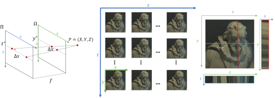
Figure 1: Light field two-plane parametrization (left), matrix of views representation (middle), and Epipolar Plane Images (EPI) representation (right).

2.2 Depth estimation from light fields

A 4D light field implicitly captures the 3D geometry of a scene. As illustrated in Figure 1, the depth $Z$ of a point $P$ in 3D space can be obtained as: $Z=-f\frac{\Delta s}{\Delta x}$, where $f$ and $\Delta s$ are respectively the focal length and the distance between camera positions, which are known parameters at the time of capture. The depth $Z$ can thus be obtained by estimating the disparity $\Delta x$.

Multiple methods taking advantage of the existing literature in stereo disparity estimation have then been proposed to estimate depth from light fields. These techniques rely on various matching approaches to estimate the disparity between views from the light field and a reference view (often the center one). In [10], the authors proposed an accurate block-matching method reaching sub-pixel accuracy based on the Fourier phase-shift theorem. To reduce the complexity, a multi-resolution approach was proposed in [19].

To better take into account the light field structure, extensions of the previous methods have been proposed based on the analysis of texture patches sampled along the angular dimensions instead of the spatial dimensions. These angular patches, also called SCam, were first exploited in [4]. This work was further extended in [25] to be robust to occlusion. More recently, this idea was included in a global optimization framework [22] in order to obtain a dense depth map estimation.

Several techniques also exploit the light field structure through EPI, as in such images the slope of a line has a linear relationship with the depth. In [26], the slope of the epipolar lines are estimated using a structure tensor, while in [28] a spinning parallelogram operator is proposed. In [12], depth from high spatio-angular resolution light fields is obtained by first estimating high confidence depth values on the EPI edges, and then propagating this information to homogeneous regions using a fine-to-coarse approach. In [11], a sparse decomposition of the EPI is performed over a depth-based dictionary built from fixed disparities, and the scene disparity is deduced from the sparse coding coefficients. In [23], defocus and correspondence cues are obtained from the EPI by shearing the epipolar lines. The shearing angle optimizing the multiple cues response gives the slope of the epipolar lines, and thus the depth.

Note that most of the aforementioned methods require an additional regularization or optimization step, which is usually a computationally intensive global process.

2.3 Optical flow

Since Horn and Schunck’s pioneer work [8] in variational optical flow estimation, many methods have been proposed exploring their idea based on energy minimization. In this subsection, we will briefly introduce the related literature in this field. For a comprehensive survey, please refer to the work in [1, 15].

The original work from [8] often leads to inaccurate estimation of large pixel displacements. To improve the accuracy of such challenging cases, the patch match method [3], initially introduced for nearest neighbor field estimation, has been adapted to the optical flow problem. Patch match provides sparse pixel correspondence, and the final optical flow estimation is then considered as a labeling problem leveraging the coherent information of natural images. To further obtain a dense flow map, Revaud et al. [20] propose an edge-preserving interpolation scheme applied on top of sparse matching correspondences. In this context, Hu et al. [9] propose a coarse-to-fine extension of the basic patch match method, which is proven efficient in finding reliable correspondences on large pixel displacements.

In addition to the spatial accuracy, the optical flow temporal consistency has been an important and challenging research topic. In their early work, Murray et al. [18], proposed to add a temporal smoothness term to improve the temporal consistency. Sliding windows [24] and Kalman filtering [6] based methods have been proposed later, focusing on temporal stability, although their performances highly rely on the selection of the window size. Feature flow [13] proposed a novel local edge-aware filtering to replace the expensive global optimization used in previous work, which significantly reduced the computation cost while performing an accurate estimation. However, this method relies on a sparse correspondence initialization, which has a significant impact on the final result.

3 Depth estimation from light fields using optical flow

3.1 System overview

In this paper, we propose a novel scheme for efficient and accurate estimation of depth maps from the 4D structure of light fields using optical flow. Our approach consists of three main steps, as illustrated in Figure 2. First, a 3D spatio-angular volume is extracted from the light field by taking views along a given angular dimension. Second, an optical flow estimation is performed over this spatio-angular volume. The displacements measured by the optical flow thus correspond to disparity estimates between consecutive views of the light field. The optical flow itself consists of two steps: an initialization with a sparse matching correspondence technique [9] is first performed, then a spatio-angular edge-aware filter is applied on the sparse estimates to obtain a dense flow estimation. For this volumetric filtering we choose the feature flow method [13]. Finally, an aggregation step is performed to obtain the depth map from the multiple disparity map estimates. A common process used in most state-of-the-art methods performs sophisticated weighted median or image guided filtering combined with costly global energy minimization on the disparity map estimates to obtain a single accurate disparity map. Thanks to the the edge-aware filtering along the angular dimension of the optical flow, which enforces the consistency between the different disparity map estimates, we can reduce this step to a simple median filtering followed by a one-step variational energy minimization. For the same reason, we can propose in this paper a novel process where several depth maps are created from each disparity map estimate, and then fused in the 3D space to create a single extra dense point cloud, which enables interesting application scenarios.

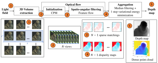
Figure 2: Overview of the proposed approach. The method can be apply on any number of rows or columns of the matrix of views in order to obtain more disparity map estimates.

3.2 3D spatio-angular volume extraction

To obtain a 3D spatio-angular volume, we fix one of the angular dimensions and extract $N$ views over the remaining dimension. This volume thus consists in a sequence of sub-aperture images, noted $V=\{I_{n}\},n=1\dots N$. Here and for the rest of this paper, we assume without loss of generality that we fix $t^{*}$ and take the sub-aperture images over $s$ (see Figure 2).

3.3 Optical flow

The optical flow method used in this paper was selected for its temporal consistency property [13]. In our context, this ensures that the different disparity estimates are consistent over the angular dimension. In addition, we propose to modify the initialization method, as described in the next section.

3.3.1 Initialization: Coarse-to-fine Patch Matching

In this paper, we propose to use a recent extension of the patch match (PM) method [3], the so-called Coarse-to-fine Patch Matching (CPM) technique as initialization [9], as it is both more efficient and accurate than the SIFT flow used in [13].

The well known PM method provides an efficient way to compute sparse matchings between a pair of images. Given two images $I_{1},I_{2}$, the goal is to find for each patch $p_{1,m}$ in $I_{1}$ a corresponding patch $p_{2,m}=\mathrm{M}(p_{1,m})$ in $I_{2}$, with $m=1\dots M$ where $M$ is the total number of patches in the image. Note that as we only look for sparse matches, $M$ is much lower than the total number of pixels. The core idea of PM is to use random search and propagation between neighbors to speed up the matching search. The matching search itself is conducted as a cost function minimization:

$$\mathrm{M}(p_{1,m})=\textup{arg}\underset{p_{2,i}}{\textup{min}}~{}C(p_{1,m},p_{2,i}),p_{2,i}\in N_{m}$$ (1)

where the cost function $C(\cdot)$ corresponds to the sum of absolute difference (SAD) of the SIFT descriptors, and $N_{m}$ is a set comprising all patches contained in a search window centered on $p_{1,m}$. Note that in our context, the sub-aperture images of a light field are rectified, and we can further reduce the complexity of the matching search by limiting the search window to an epipolar line.

The CPM method then consists in applying PM on a hierarchical architecture. A pyramid with $k$ levels is first constructed from the original images with a downsampling factor $\eta$. This pyramidal decomposition is noted $I_{i}^{l}$ with $i=1,2$ and $l=1\dots k$. The PM method is first applied on the $I_{1}^{k}$ and $I_{2}^{k}$ with a random initialization, and then iteratively on $I_{1}^{l}$ and $I_{2}^{l}$ with $l=k-1\dots 1$ using the output of the previous level $l+1$ as initialization.

To initialize our optical flow, we apply the CPM method on consecutive pairs of views $I_{n},I_{n+1}$ with $n=1\dots N-1$ taken from the volume $V$ built previously, and we note $f_{n}^{init}$ the flow between these views.

3.3.2 Efficient spatio-angular filtering: Feature flow

Once sparse matches are obtained as described in previous section, we performed edge-aware filtering on the spatio-angular volume in order to obtain dense consistent correspondences. We introduce in this section the feature flow method [13], an efficient edge-aware filter, used to diffuse sparse matches with coherent information. One of the main advantage of the feature flow is that the global energy minimization operation used in many optical flow approaches is replaced with a local volumetric edge-aware filtering operation. To properly detect object edges in sub-aperture images and their disparity variations, a domain transform filter [5] is applied iteratively on the 3 spatio-angular dimensions with a fixed width Gaussian kernel. The flow $f_{n}$ between views $I_{n},I_{n+1}$ is obtained from the flow from previous views as $f_{n}=G*f_{n-1}$ where $G$ is the domain transform filter mentioned above and $*$ is a convolution operator. Note that the filtering along the angular dimension follows "disparity paths" provided by the initial sparse flow estimations $f_{n}^{init}$, with $n=1\dots N-1$.

To improve the accuracy of the flow estimation, the input sparse flow is weighted with a confidence map, whose weights are computed as the absolute difference between the matching correspondence vectors, thus increasing the contribution of reliable matches.

3.4 From disparity to depth map

3.4.1 Single accurate disparity map

The first approach to obtain the final depth map is to first compute a single disparity map from all estimates, which is then converted into a depth map $Z_{init}$ using the equation from Section 2.2. This technique is used in many state-of-the-art methods, e.g. based on weighted median or image guided filtering, which efficiently removes outliers, and is often followed by a costly global energy minimization technique.

However, thanks to the angular filtering which enforce the consistency between the different disparity map estimates, we can apply a much simpler and faster aggregation step, using median filtering and a one-step variational energy minimization. Here, the one-step variational energy minimization from the Epicflow [20] method is used to obtain the final depth map $Z_{f}$ from $Z_{init}$:

$$Z_{f}=\textup{arg}\underset{Z_{i}}{\textup{min}}(E_{data}(Z_{i})+\lambda\alpha E_{smooth}(Z_{i}))$$ (2)

where $E_{data}$ corresponds to a classical color-constancy data term while $E_{smooth}$ corresponds to a gradient-constancy function with a local smoothness term weight $\alpha=exp(-\kappa\left\|\nabla_{2}Z\right\|)$ [27], where $\kappa=5$.

3.4.2 Extra dense Point Cloud

Thanks to the consistency of the different disparity estimates, we can use a novel process to create the point cloud, where multiple point clouds are created from each disparity map, and then aggregated in the 3D space to obtain the final extra dense point cloud.

4 Evaluation

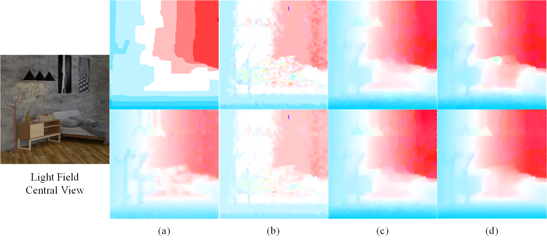
Figure 3: Comparison of optical flow obtained with state-of-the-art methods. Top row consists of initialization results with different optical flow methods. Bottom row is the results of these initializations + feature flow filter. (a) SIFT Flow [16] (4.9s); (b) EPPM [2] (GPU-based,0.7s); (c) EpicFlow [20] (15s); (d) CPM-Flow [9] (5.3s) (Best viewed in color)

In this section, we analyze the results of the proposed approach. All our experiments were run on an Intel Core i7-6700k 4.0GHz CPU. We use the feature flow implementation from [21] and the same parameter setting for all our experiments. For the CPM method, the level of pyramids $k$ is set to 5, the downsampling factor $\eta$ is set to the 0.5 and the patch size is set to 3x3.

Evaluation of the optical flow. We evaluate here the performance of the proposed optical flow approach against state-of-the art methods. In Figure 3, we show the results of several optical flow initializations in the top row and the results after feature flow filtering in the bottom row. The volumetric filtering using feature flow along the angular dimension of the light field clearly improves the accuracy of the optical flow from any initialization method, significantly improving consistency and continuity of brightness. The proposed method using CPM as initialization achieves the best performance in terms of balance between speed and accuracy.

The importance of the volumetric filtering is also illustrated in Figure 6, where we show the final depth map results for several light fields obtained with our method with and without feature flow. The quality of the depth maps is clearly improved with feature flow for all sequences.

HCI benchmark performance. We evaluate here the accuracy and efficiency of our proposed method against state-of-the-art light field depth map estimation methods [26, 11, 28, 25, 10, 22, 19] using the recent HCI 4D light field dataset [7] . The accuracy of the depth estimation is evaluated using the Mean Square Error (MSE) * 100 and the computational complexity using the running time in seconds. The results are summed up in the graph of Figure 4, showing the average performances over the HCI dataset. More detailed results will be made available on our web page. Our method achieves comparable perfomance with the best method of the state-of-the-art in terms of balance between accuracy and speed.

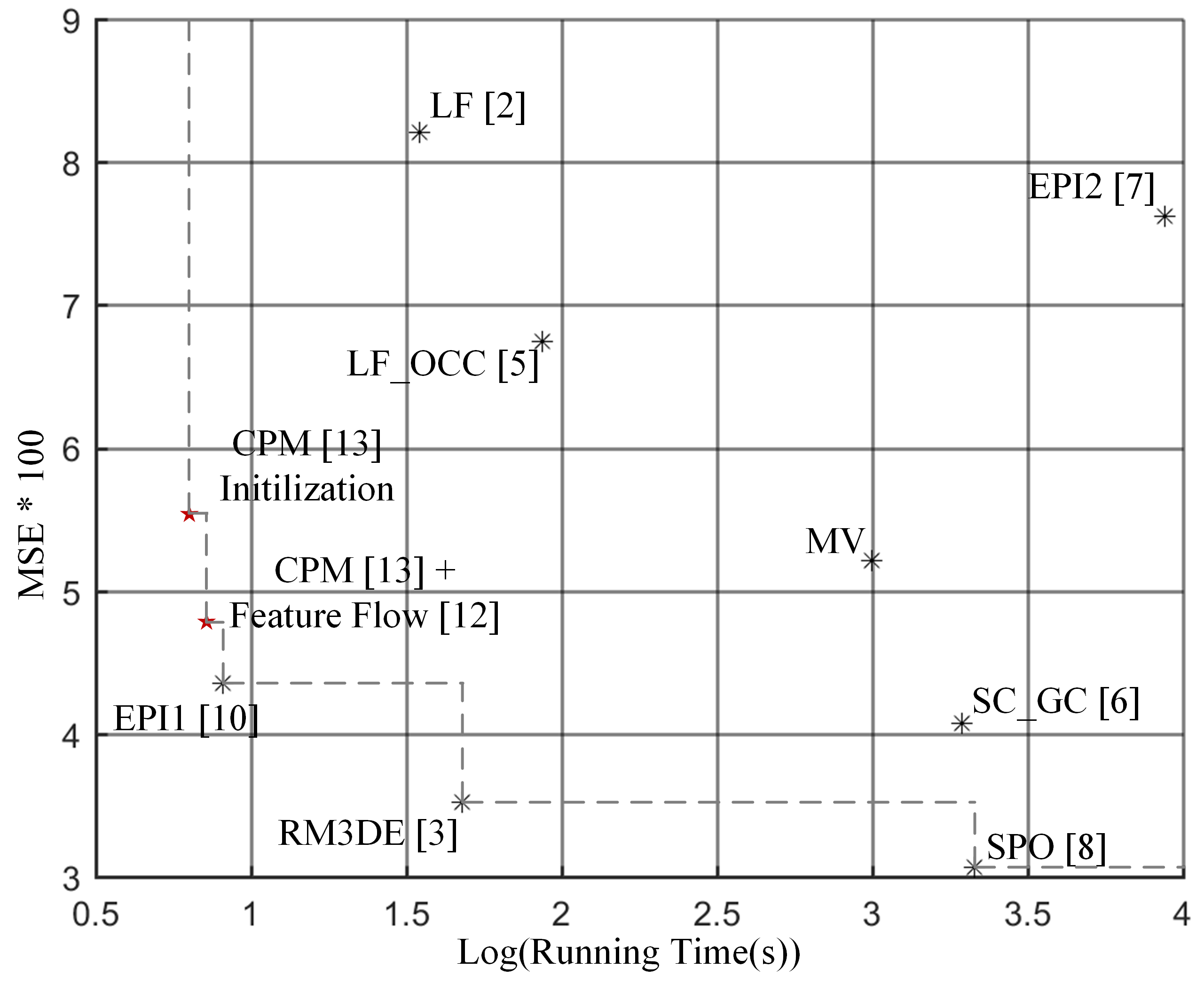
Figure 4: Comparison of our method (red stars) performances against state-of-the-art (blue stars), averaged over all HCI light fields. The results show that we achieve comparable performances to the best state-of-the-art method in terms of balance between speed and accuracy.

In addition to these objective metrics, we show the depth maps obtained from several light fields in Figure 6 and compare against state-of-the-art methods. The final comparison shows better performance for edge preservation of objects (see Cotton column) and also smoother results for noisy scenes (see Backgammon and Dino columns). However, we notice that the proposed local filtering method, which allows considerable speed up, sometime produces less smooth results than a global solution (see background of Dino and Boxes column). The feature flow filter also heavily depends on the quality of the optical flow initialization. If the optical flow method is unable to provide accurate correspondence, it can not be corrected by the filter (see for example the Boxes column).

Note that at the time of writing, some recent results were added in the HCI benchmark without any attached publications. As we can not fully understand and exploit comparisons with methods which are not described, we choose in this paper to compare our results only against published work.

Extra dense 3D Point Cloud. As mentioned in Section 3.4, a unique feature of our method compared to the state-of-the-art approaches is that we can produce several consistent depth maps which can then be integrated in the 3D space in order to produce extra dense point clouds. Examples of such results are shown in Figure 5 in comparison with point clouds obtained with a single depth map.

5 Conclusion

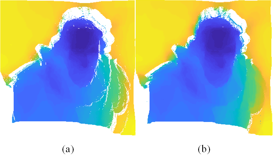
Figure 5: (a) Single point clouds (about 260k points) v.s. (b) Extra dense point clouds (more than 21 million points). (Best viewed in color)

In this paper, we introduced a novel optical flow-based method to estimate depth maps from light fields. We showed that by extracting a 3D volume consisting of a sequence of views from the 4D light field, and applying a temporally consistent optical flow on this spatio-angular volume, we were able to obtain high-quality depth maps with a reduced complexity. Comparison with state-of-the-art methods on the HCI benchmark showed that we are competitive with the best method in terms of balance between accuracy and speed. Furthermore, thanks to the enforced consistency of the disparity map estimates along the angular dimension, we are able to produce point clouds with a much higher density than in any state-of-the-art method. However, we note that our local filtering sometimes yield inferior results compared to global optimizations. In future work, we plan to investigate different spatio-angular filtering methods in order to improve the accuracy while keeping a faster running time. Furthermore, we intend to apply our method on dense light fields captured with lenslet cameras such as Lytro [17] to perform 3D reconstruction of real world scenes.

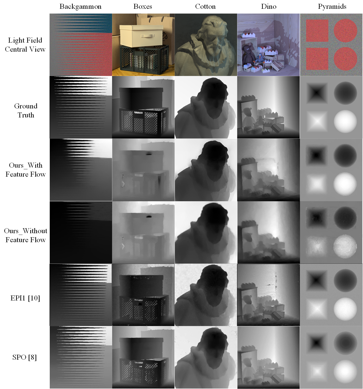
Figure 6: Depth map comparison on HCI dataset

References

- [1] Simon Baker, Daniel Scharstein, J. P. Lewis, Stefan Roth, Michael J. Black, and Richard Szeliski. A database and evaluation methodology for optical flow. International Journal of Computer Vision, 92(1):1–31, 2011.
- [2] Linchao Bao, Qingxiong Yang, and Hailin Jin. Fast edge-preserving patchmatch for large displacement optical flow. In Proceedings of the IEEE Conference on Computer Vision and Pattern Recognition, pages 3534–3541, 2014.
- [3] Connelly Barnes, Eli Shechtman, Adam Finkelstein, and Dan Goldman. Patchmatch: A randomized correspondence algorithm for structural image editing. ACM Transactions on Graphics-TOG, 28(3):24, 2009.
- [4] Can Chen, Haiting Lin, Zhan Yu, Sing Bing Kang, and Jingyi Yu. Light field stereo matching using bilateral statistics of surface cameras. In Proceedings of the IEEE Computer Society Conference on Computer Vision and Pattern Recognition, pages 1518–1525, 2014.
- [5] Eduardo SL Gastal and Manuel M Oliveira. Domain transform for edge-aware image and video processing. ACM Transactions on Graphics (ToG), 30(4):69, 2011.
- [6] Matthias Hoeffken, Daniel Oberhoff, and Marina Kolesnik. Temporal prediction and spatial regularization in differential optical flow. In International Conference on Advanced Concepts for Intelligent Vision Systems, pages 576–585. Springer, 2011.
- [7] Katrin Honauer, Ole Johannsen, Daniel Kondermann, and Bastian Goldluecke. A dataset and evaluation methodology for depth estimation on 4d light fields. In Asian Conference on Computer Vision. Springer, 2016.
- [8] B.K.P. Horn and B.G. Schunck. Determining optical flow. Artificial intelligence, 17(1-3):185–203, 1981.
- [9] Yinlin Hu, Rui Song, and Yunsong Li. Efficient coarse-to-fine patchmatch for large displacement optical flow. In Proceedings of the IEEE Conference on Computer Vision and Pattern Recognition, pages 5704–5712, 2016.
- [10] Hae Gon Jeon, Jaesik Park, Gyeongmin Choe, Jinsun Park, Yunsu Bok, Yu Wing Tai, and In So Kweon. Accurate depth map estimation from a lenslet light field camera. Proceedings of the IEEE Computer Society Conference on Computer Vision and Pattern Recognition, 07-12-June:1547–1555, 2015.
- [11] Ole Johannsen, Antonin Sulc, and Bastian Goldluecke. What Sparse Light Field Coding Reveals about Scene Structure. In 2016 IEEE Conference on Computer Vision and Pattern Recognition (CVPR), pages 3262–3270. IEEE, June 2016.
- [12] Changil Kim, Henning Zimmer, Yael Pritch, Alexander Sorkine-Hornung, and Markus Gross. Scene reconstruction from high spatio-angular resolution light fields. ACM Trans. Graph., 32(4):73:1–73:12, July 2013.
- [13] Manuel Lang, Oliver Wang, Tunc Aydin, Aljoscha Smolic, and Markus Gross. Practical temporal consistency for image-based graphics applications. ACM Transactions on Graphics (ToG), 31(4):34, 2012.
- [14] Marc Levoy and Pat Hanrahan. Light field rendering. In Proceedings of the 23rd Annual Conference on Computer Graphics and Interactive Techniques, SIGGRAPH ’96, pages 31–42, 1996.
- [15] Wenbin Li, Yang Chen, JeeHang Lee, Gang Ren, and Darren Cosker. Robust optical flow estimation for continuous blurred scenes using rgb-motion imaging and directional filtering. In Applications of Computer Vision (WACV), 2014 IEEE Winter Conference on, pages 792–799. IEEE, 2014.
- [16] Ce Liu, Jenny Yuen, Antonio Torralba, Josef Sivic, and William Freeman. Sift flow: Dense correspondence across different scenes. Computer vision–ECCV 2008, pages 28–42, 2008.
- [17] The lytro illum camera. https://www.lytro.com/imaging. accessed: 23-05-2017.
- [18] David W Murray and Bernard F Buxton. Scene segmentation from visual motion using global optimization. IEEE Transactions on Pattern Analysis and Machine Intelligence, 1(2):220–228, 1987.
- [19] Alessandro Neri, Marco Carli, and Federica Battisti. A multi-resolution approach to depth field estimation in dense image arrays. Proceedings - International Conference on Image Processing, ICIP, 2015-Decem:3358–3362, 2015.
- [20] Jerome Revaud, Philippe Weinzaepfel, Zaid Harchaoui, and Cordelia Schmid. Epicflow: Edge-preserving interpolation of correspondences for optical flow. In Proceedings of the IEEE Conference on Computer Vision and Pattern Recognition, pages 1164–1172, 2015.
- [21] Joan Sol Roo and Christian Richardt. Temporally coherent video de-anaglyph. In ACM SIGGRAPH 2014 Posters, page 75. ACM, 2014.
- [22] Lipeng Si and Qing Wang. Dense Depth-Map Estimation and Geometry Inference from Light Fields via Global Optimization, pages 83–98. Springer International Publishing, 2017.
- [23] Michael W. Tao, Sunil Hadap, Jitendra Malik, and Ravi Ramamoorthi. Depth from combining defocus and correspondence using light-field cameras. Proceedings of the IEEE International Conference on Computer Vision, 2:673–680, 2013.
- [24] Sebastian Volz, Andres Bruhn, Levi Valgaerts, and Henning Zimmer. Modeling temporal coherence for optical flow. In Computer Vision (ICCV), 2011 IEEE International Conference on, pages 1116–1123. IEEE, 2011.
- [25] Ting-Chun Wang, Alexei A. Efros, and Ravi Ramamoorthi. Occlusion-Aware Depth Estimation Using Light-Field Cameras. 2015 IEEE International Conference on Computer Vision (ICCV), pages 3487–3495, 2015.
- [26] Sven Wanner and Bastian Goldluecke. Globally consistent depth labeling of 4D light fields. In 2012 IEEE Conference on Computer Vision and Pattern Recognition, pages 41–48. IEEE, June 2012.
- [27] Li Xu, Jiaya Jia, and Yasuyuki Matsushita. Motion detail preserving optical flow estimation. IEEE Transactions on Pattern Analysis and Machine Intelligence, 34(9):1744–1757, 2012.
- [28] Shuo Zhang, Hao Sheng, Chao Li, Jun Zhang, and Zhang Xiong. Robust depth estimation for light field via spinning parallelogram operator. Computer Vision and Image Understanding, 145:148–159, 2016.