Ionisation rate and Stark shift of a one-dimensional model of the Hydrogen molecular ion

Abstract

In this paper we study the ionization rate and the Stark shift of a one-dimensional model of the H${}_{2}^{+}$ ion. The finding of these two quantities is reduced to the solutions of a complex eigenvalue problem. We solve this problem both numerically and analytically. In the latter case we consider the regime of small external electrostatic fields and small internuclear distances. We find an excellent agreement between the ionization rate computed with the two approaches, even when the approximate result is pushed beyond its expected validity. The ionization rate is very sensitive to small changes of the external electrostatic field, spanning many orders of magnitude for small changes of the intensity of the external field. The dependence of the ionization on the internuclear distance is also studied, as this has a direct connection with experimental methods in molecular physics. It is shown that for large distances the ionization rate saturates, which is a direct consequence of the behavior of the energy eigenvalue with the internuclear distance. The Stark shift is computed and from it we extract the static polarizability of H${}_{2}^{+}$ and compare our results with those found by other authors using more sophisticated methods.

1 Introduction

The quantum study of the hydrogen molecular ion is almost as old as quantum mechanics itself [1]. This molecular ion is the simplest system we can think of in molecular physics. It consists of a three body fermionic problem, where two of the fermions are the identical protons and the third one is the electron binding the two protons together. This system configures a three-body problem. The wave functions, energy levels, and equilibrium distances are known from numerical calculations [2] or from variational approaches [3, 4, 5, 6]. When acted upon by a static electric field the system can ionize following two different channels [7, 8]: (i) the Coulomb explosion channel (or ionization channel), where the reaction has the form $\mathrm{H}_{2}^{+}\rightarrow p+p+e$; (ii) the dissociation channel, where the reaction form has the form $\mathrm{H}_{2}^{+}\rightarrow p+\mathrm{H}$. These two channels have different probabilities to occur, depending on whether we are considering an electrostatic field or a laser field, from which a number of photons can be absorbed.

The motion of the three particles involved in the dynamics of the $\mathrm{H}_{2}^{+}$ ion can be separated in two different types of motion: (i) slow motion of the heavy protons; (ii) the fast motion of the electron. As noted, solving the three-body problem considering the motion of the three particles in the same footing is virtually impossible from an analytical point of view. However, because of the two very different time scales involved in the motion dynamics we can separate the motion of the protons from the motion of the electron. This approach is at the heart of the Born-Oppenheimer approximation. Therefore, one usually considers a time interval where the protons’ motion is frozen and the electron dynamics is considered as the only relevant process.

Taking into account the Born-Oppenheimer approximation, analytical expressions for the ground state wave function of $\mathrm{H}_{2}^{+}$ are obtained using an appropriate set of coordinates [4]. The ionization of the ion requires adding an extra term to the Hamiltonian that describing the interaction of the electron with the static electric field. This apparently simple term, linear in position, immediately renders the molecular problem intractable, even within the Born-Oppenheimer approximation. This is a consequence of the known difficulty of solving the Coulomb problem in the presence of an external electric field [9].

All the aforementioned difficulties can be overcome by studying simpler models, which still contain the basic physical traits of the problem. It is in this context that simpler one-dimensional models [10, 11, 12, 13, 14, 15, 16, 17, 18, 19, 20, 21, 22, 6, 23] are usually proposed for studying the ionization of atoms and molecules by static electric fields. In these types of models, the Coulomb interaction is replaced by a short range potential, typically a Dirac $\delta$-function potential, whose strength is adjusted to produce the observed ionization energy of the atom or molecule in case (see procedure further down in the text). In addition to this, the coupling to the external electrostatic field is added via the dipole approximation. These models are much simpler than the Coulomb problem, since the short range nature of the potential guaranties that the effect of the external field can be obtained exactly.

Many different problems related to this topic have been studied. As mentioned above, approaches based on numerical and variational methods have been implemented. Methods based on cylindrical [2], elliptic [4] and parabolic [24] coordinates have been used. Ionization by static and laser fields [25, 18, 26] has been analyzed. In addition, the use of sum rules has been considered to study the problem of a single $\delta-$function in Ref. [27] and the problem of dissociation and Stark effect in non-rigid dipolar molecules in Ref. [28]. The delta function approach to the Coulomb potential in 1D has been used by many authors. In Ref.[25] the problem of a $\delta-$function potential in a strong field is treated numerically. In Ref. [14], absolutely convergent periodic-orbit expansion techniques are used to obtain an analytical solution for the compressed Hydrogen atom, where the finite-range Coulomb potential is replaced by a zero-range $\delta-$function potential. In Ref. [23] a simple model of a diatomic ion using $\delta-$functions is compared with more complex methods. The $\delta-$function potential has also been used to unveil the optical response of one-dimensional semiconductors, that is the response to an electric field oscillating in time [29].

The success of the $\delta-$function potential to describe the basic physics of Coulomb explosion of simple molecules and ions has been so impressive that we follow the same path in this paper and analyze a different approach to the calculation of the ionization rate of the $\mathrm{H}_{2}^{+}$ ion, which has not been considered before in the literature to our best knowledge.

The paper is organized as follows: in Sec. 2 we introduce the molecular-ion model, which has already been studied by many authors, mainly to defined the problem and to fix the notation used throughout the paper. In Sec. 3, the ionization rate and the Stark shift for our one-dimensional ion model are computed. In Sec. 4 we give a summary of our results.

2 Model

In this section, we introduce the model for the molecular ion and define the different quantities used throughout the text. We start solving the problem in the absence of an external static electric field, thus computing the bound states of the system. When an external electric field is present the bound states become quasi-bound states, presenting an energy shift relative to the zero field case, as well as a finite spectral width. This will be studied in the next section.

The Schrödinger equation, in atomic units, describing our one-dimensional model of the H${}_{2}^{+}$ ion reads

$$-\frac{d^{2}}{dx^{2}}\psi(x)-W\left[\delta(x-a)+\delta(x+a)\right]\psi(x)+Fx\psi(x)=-\kappa^{2}\psi(x),$$ (1)

where $W=2\mu Z$ (with $Z$ playing the role of the nuclear charge), $F=2\mu\lambda$ (playing the role of the electric force), and $\kappa^{2}=-2\mu E$, with $E$ the binding energy associated with the wave function $\psi(x)$. Both $W$ and $F$ are positive quantities, and $E<0$ when $F\rightarrow 0$ but is otherwise a complex number. he quantities $\mu$, $Z$, $\lambda$, and $a$ refer to the reduced mass, potential strength or nuclear charge, force field strength, and half the internuclear separation (half the proton-proton distance), respectively. In the Born-Oppenheimer approximation, where the electronic and nuclear motions are decoupled, this equation can be seen as a one-dimensional model of a homo-nuclear diatomic molecule, such as $\mathrm{H}_{2}^{+}$. In this particular case, the two protons have an equilibrium distance given by $2a$, and the single electron experiences two $\delta-$like potentials associated with each of the two protons. This specific example will be the object of our attention later in the text. In a more realistic model, the single electron should interact with the two protons through the Coulomb interaction. However, these two potentials, the $\delta-$function potential and the Coulomb potential, share some common features, namely: both diverge at the origin; the virial theorem is the same in both cases [17], and both respect the property $xV^{\prime}(x)=-V(x)$, with $V(x)=\delta(x)$ or $1/|x|$. These similarities, combined with the simplicity the $\delta-$function potential brings to the problem, make this a popular choice to model 1D systems. With this said, one should keep in mind that the $\delta-$function potential is still significantly different from the Coulomb potential, which inevitably reduces the accuracy of the final results.Still, previous works report a fair agreement between the $\delta-$function and the Coulomb potential, when both are used to model the same system [19]. One way to overcome the differences between the $\delta-$function potential and Coulomb potential is to ascribe a value for $W$ that reproduces the ground state energy of the Coulomb potential (this is the strategy we use later in the paper).

We now focus on the case where the external electric field is absent, that is $F=0$. In this case, when $x\neq\pm a$, the general solution of the Schrödinger equation corresponds to a superposition of real valued exponentials

$$\psi(x)=Ae^{\kappa x}+Be^{-\kappa x},$$ (2)

with $A$ and $B$ some coefficients determined by the constraints of the problem, such as boundary conditions, continuity, and normalization. The three different regions of our system will present particular cases of this general solution. For $x<-a$ in order to have a finite wave function, only the exponential with a positive argument can exist. Following the same reasoning, for $x>a$ only the exponential with a negative argument is allowed to be present. In the middle region, $-a<x<a$, we use the symmetry of the system with respect to the origin to state that the wave functions must have either even or odd parity, that is, $\psi(x)=C\cosh(\kappa x)$ or $\psi(x)=C\sinh(\kappa x)$, respectively, with $C$ some constant. These two cases have to be studied separately. The introduction of a specific parity to our solution simplifies the problem, since now we only need to study the boundary conditions at either $a$ or $-a$.

Imposing the continuity of $\psi(x)$ at $x=a$, $\psi(a^{+})=\psi(a^{-})$, as well as the discontinuity of its derivative, which is a direct consequence of the $\delta-$functions in the Schrödinger equation, $\psi^{\prime}(a^{+})-\psi^{\prime}(a^{-})=-W\psi(a)$, one obtains a system of two equations with two unknowns. In order to guarantee the existence of non-trivial solutions, we require the determinant of the system to vanish. From here an implicit relation defining the binding energy in the absence of the electric field is obtained as

$$\tanh(\kappa_{0}^{\mathrm{even}}a) = \frac{W}{\kappa_{0}^{\mathrm{even}}}-1,$$ (3)

$$\coth(\kappa_{0}^{\mathrm{odd}}a) = \frac{W}{\kappa_{0}^{\mathrm{odd}}}-1,$$ (4)

where $\kappa_{0}^{{\rm even/odd}}=\sqrt{-2\mu E_{0}^{{\rm even/odd}}},$ with $E_{0}^{{\rm even/odd}}$ the energy, in the absence of the field, of the even/odd solution. Equations (3) and (4) define two real eigenvalue problems. From the inspection of the two previous relations we note that the first one, related to the even case, always has a solution. However, the second one, associated with the odd wave function, only has a solution when $aW>1$. This is easily understood from the asymptotic behavior of the equation. When $\kappa_{0}^{\mathrm{odd}}a\rightarrow 0$, the left hand side diverges as $\coth(\kappa_{0}^{\mathrm{odd}}a)\sim 1/\kappa_{0}^{\mathrm{odd}}a$ while the right hand side goes as $aW/\kappa_{0}^{\mathrm{odd}}a$. In the opposite limit, when $\kappa_{0}^{\mathrm{odd}}a\rightarrow\infty$, the left hand side approaches $1$, while the right hand side approaches $-1$. In order to find a solution both sides of the equation have to intercept at some specific value of $\kappa_{0}^{\mathrm{odd}}a$. This is only possible if the right hand side is more divergent than the left hand side when $\kappa_{0}^{\mathrm{odd}}a\rightarrow 0$, which is equivalent to saying that a solution only exists when the condition $aW>1$ is fulfilled. Finally we observe that as $a$ increases the energies of the odd and even states get closer to each other and to the saturation value $-W^{2}/2\mu$. Saying it differently, the bonding and anti-bonding molecular orbitals separate from each other as the internuclear distance is decreased due to hybridization of the two atomic orbitals.

3 Ionization rate and Stark shift

In this section, we draw inspiration from Ref. [12] to extend the previous discussion to the case where the external electric field is present. In the first part of this section we will obtain an approximate analytical expression for the Stark-shift and the ionization rate. Afterwards, we will focus on the specific case of the hydrogen molecule ion $\mathrm{H}_{2}^{+}$ and study how the Stark-shift and ionization rate depend on the parameters of the system. In the end, we will compute the static polarizability and compare it with previously published results, both theoretical and experimental.

In the presence of an external electric field, $F\neq 0$, the Schrödinger equation when $x\neq\pm a$ becomes

$$\frac{d^{2}}{dx^{2}}\psi(x)-F\left(x+\frac{\kappa^{2}}{F}\right)\psi(x)=0.$$ (5)

With the change of variable $y=F^{1/3}(x+\kappa^{2}/F)$, the equation can be cast in the form

$$\frac{d^{2}}{dy^{2}}\psi(y)-y\psi(y)=0,$$ (6)

which is nothing but the Airy differential equation, whose solution is a superposition of the Airy functions $\mathrm{Ai}(y)$ and $\mathrm{Bi}(y)$ [30, 31]. We can now proceed in a similar way to what was done in the previous section, only this time we will be working with Airy functions instead of real valued exponentials, a clear sign of the change of behavior of the system in the presence of an external electrostatic field. The main difficulty relatively to what was done before is that, in the presence of the external electrostatic field, we can no longer use the parity of the wave function to simplify the problem. This implies that the boundary conditions have to be evaluated at both $x=a$ and $x=-a$, transforming the problem into a more involved one.

Let us now briefly go over the reasoning behind solving Eq. (6) in the three different regions of the system. As was said before, the solution of the Airy equation will be a superposition of Airy functions, so, in the region $x<-a$, the wave function has the general form

$$\psi(y)=A\mathrm{Ai}(y)+B\mathrm{Bi}(y),$$ (7)

In the previous section, we were able to simplify the solution in this region by looking at the limit $x\rightarrow-\infty$ and demanding the wave function to be finite. In the present scenario, the same limit proves to be useful, although the employed physical argument differs slightly. In the presence of an electrostatic field, when $x\rightarrow-\infty$, the wave function has to present a traveling wave nature. From the appropriate series expansion of both Airy functions, we see that $\mathrm{Ai}(y)$ and $\mathrm{Bi}(y)$ are proportional to sines and cosines, respectively. We thus see that in order to recover a traveling wave in the $x\rightarrow-\infty$ limit, the superposition coefficients $A$ and $B$ have to be related as $A=iB$. In the opposite region, where $x>a$, the solution is once more a superposition of Airy functions that can be simplified upon analysis of the correct limiting case. Studying the limit $x\rightarrow\infty$, we note that the Airy function $\mathrm{Bi}(y)$ is proportional to the real valued exponential $e^{y}$. Since this asymptotic behavior would lead to a divergence of the wave function, it is clear that the coefficient associated with $\mathrm{Bi}(y)$ must vanish. Finally, in the intermediate region, $-a<x<a$, we once again find the solution to be a superposition of Airy functions, only this time there are no symmetry or physical arguments that allow us to relate the coefficients of the superposition, and the general solution has to be used.

With the wave function found in the three regions of interest, apart from some undetermined constants, we can formulate a complex eigenvalue problem, from which the value of the energy of the quasi bound state can be obtained. Applying the boundary conditions at $x=a$ and $x=-a$, and requiring the determinant of the resulting system to vanish, we find the following implicit relation defining the eigenenergy as

$$\frac{F^{2/3}}{W\pi} = F^{1/3}\mathrm{Ai}(y_{a})\mathrm{Ci}(y_{a})+F^{1/3}\mathrm{Ai}(y_{-a})\mathrm{Ci}(y_{-a})$$ (8)

$$+ W\pi\mathrm{Ai}^{2}(y_{a})\mathrm{Bi}(y_{-a})\mathrm{Ci}(y_{-a})-W\pi\mathrm{Ai}(y_{a})\mathrm{Ai}(y_{-a})\mathrm{Bi}(y_{a})\mathrm{Ci}(y_{-a}),$$

with $y_{\pm a}=F^{1/3}(\pm a+\kappa^{2}/F)$ and $\mathrm{Ci}(z)=\mathrm{Bi}(z)+i\mathrm{Ai}(z)$. In order to arrive at this result it was useful to consider the identity $\mathrm{Ai}(z)\mathrm{Bi}^{\prime}(z)-\mathrm{Ai}^{\prime}(z)\mathrm{Bi}(z)=1/\pi$, which is nothing but the Wronskian of the two Airy solutions. Equation (8) has a higher degree of complexity than the one found for the problem of a single $\delta-$function [12]. The increased difficulty arises from the necessity of evaluating the boundary conditions at two different coordinates, which transforms the eigenvalue problem from a $2\times 2$ to a $4\times 4$ matrix problem. Although Eq. (8) can be solved exactly numerically, an analytical solution is not readily available and is highly desirable. In order to find one, we will look at the weak field limit $F\ll 1$ (also corresponding to $y_{\pm a}\gg 1$), and follow a perturbative approach. We now introduce the following series representation of the Airy functions in the limit of interest [30, 31]

$$\mathrm{Ai}(z) \sim\frac{1}{2\sqrt{\pi}}z^{-1/4}e^{-\zeta}\sum_{k=0}^{\infty}(-1)^{k}\zeta^{-k}c_{k},\quad\zeta=\frac{2}{3}z^{3/2}$$ (9)

$$\mathrm{Bi}(z) \sim\frac{1}{\sqrt{\pi}}z^{-1/4}e^{\zeta}\sum_{k=0}^{\infty}c_{k}\zeta^{-k},$$ (10)

where

$$c_{0}=1\quad c_{k}=\frac{\Gamma(3k+1/2)}{54^{k}k!\Gamma(k+1/2)},\quad k>0.$$ (11)

To continue with the calculation we insert the series expansions into Eq. (8). From the simultaneous analysis of the series expansions and of Eq. (8), one clearly sees that, even if only the zero–th order term of each series was considered, a compact solution to the eigenvalue equation would still be elusive due to the pre-factors in Eqs. (9) and (10). With this difficulty in mind, we introduce the first approximation in our procedure by substituting all the $y_{\pm a}$ that appear in the pre-factors by $y_{0}=\kappa^{2}/F^{2/3}$. Although at first sight this may seem too crude an approximation, the fact that we will be concerned with the weak field limit justifies this approach, since we can expect $\kappa^{2}/F$ to be considerably larger than $a$, and thus $y_{\pm a}\approx y_{0}$ for a small enough field strength. Furthermore, we stress that this approximation is only applied to the pre–factors, and not to the exponentials, where even a small change in the argument could still lead to a significant difference in the final result. This approximation simplifies our problem, since we were now able to isolate a single $\kappa$ (which is directly linked to the energy) on one side of the equation. After this is done, one approximation remains: all the $\kappa$ that appear on the opposite side of the equation are substituted by their value in the absence of the electrostatic field, $\kappa_{0}$, as given in Eq. (3). Considering only the lowest order terms in the different sums, a simple compact expression for $\kappa$ is reached, which reads

$$\kappa\approx W + i\frac{W}{4}\left(1+\frac{W}{2\kappa_{0}}\right)e^{-\frac{4}{3F}\left(\kappa_{0}^{2}Fa\right)^{3/2}}$$ (12)

$$+ i\frac{W}{4}\left(1-\frac{W}{2\kappa_{0}}\right)We^{-\frac{4}{3F}\left(\kappa_{0}^{2}-Fa\right)^{3/2}},$$

from which the energy $E$ can be obtained if one recalls that $\kappa=\sqrt{-2\mu E}$. The real part of $E$ gives the energy of the Stark shifted energy level, while the imaginary part yields the ionization rate $\Gamma$ according to the relation $\Gamma=-2\mathrm{Im}E/\hbar$. A comment on the quality of this approximate result is now in order. As we will shortly see, this result produces an excellent description of the ionization rate as a function of the field strength $\lambda$ and as a function of the internuclear distance $2a$. However, the same cannot be said regarding the real part of the energy. On the one hand, the lowest order approximation, although acceptable for the ionization rate, fails to capture any information regarding the dependence of the Stark shift on the field (below we show how to improve the value of real part of the energy); for that to happen, higher order field terms must be introduced in the calculation. On the other hand, the zero–th order term, which can be seen from Eq. (12) to be $\kappa=W$, or $E=-W^{2}/2\mu$, does not correspond to the exact energy of the bound state in the absence of the field. In fact, this is the energy we would obtain from Eq. (3) if we took the limit $a\rightarrow 0$. It is important to note that, since the binding energy in the absence of the field is given by an implicit relation, Eq. (3), one should not expect to find the correct zero–th order term with the approach we followed, contrary to what would happen if the problem of a single atom was treated [12], since in this case the analytical expression for the energy of the ground state is known. Indeed, only the limit $a\rightarrow 0$ should appear, which is exactly what we find. However, when higher order terms are included, the Stark shift (to be discussed below) should be accurately determined, which, as we will see, it is.

Let us now explicitly put Eq. (12) to the test by applying it to the case of the Hydrogen molecular ion. To do so, we will consider the parameters given in Table 1.

$\mu$ ($m_{0}$)	$a$ ($a_{0}$)	$Z$ ($E_{h}a_{0}$)	$E_{0}^{\mathrm{even}}$ (eV)
1	1	0.99	$-16.45$

Table 1: Parameters used to model the Hydrogen molecular ion. The reduced mass $\mu$ was set equal to $1$ bare electron mass ($m_{0})$, the equilibrium length 2$a$ was chosen to be equal to 2 Bohr radii ($a_{0})$, and the potential strength was chosen as $0.99$ $E_{h}a_{0}$ (with $E_{h}$ corresponding to the Hartree unit). This choice of $a$ and $Z$ reproduces the total energy of H${}_{2}^{+}$ (which we associate with the ground state energy of the electron in the ion), which is known to be equal to $-16.45$ eV, according to Ref. [32]. Also, the equilibrium internuclear distance of $2a=2a_{0}$ is in agreement with what is known for the ground state of H${}_{2}^{+}$[33, 34, 32].

In panel a of Fig. 1, we depict the ionization rate as a function of the field strength $\lambda$ from the numerical solution of Eq. (8) and from the analytical expression given in Eq. (12), for different values of $a$. There we observe an excellent agreement between the approximate analytical expression and the exact numerical results, even for values of $a\sim 1$, which are beyond the expected validity limit of our approximation. The ionization rate spans vast orders of magnitude over a small range of field strengths, emphasizing the extreme sensitivity of the former relative to the latter. Moreover, we note that the ionization rate increases with increasing $a$ for the same field strength. This is a result at the reduced binding energy. For higher values of $a$ this increase becomes less noticeable. In fact, we found reasonable results even for $a>1$, but due to its similarity with the already depicted cases, we chose not to present them. In the panel b of the same figure, we study the dependence of the ionization rate on the position $a$ of the protons, for three different values of the field strength. This is a relevant behavior to study due to its appearance in experimental works [35, 36]. Once more, the agreement between the numerical and analytical results is self–evident. Furthermore, we observe a saturation of the ionization rate as $a$ increases, which is consistent with the behavior of the binding energy as a function of $a$, which tends for a finite value , $E=-W^{2}/(2\mu)$, when $a\gg 1$. Again we note that the agreement between the data sets extends beyond the expected validity region.

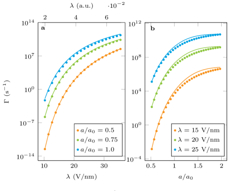
Figure 1: Ionization rate of the one dimensional H${}_{2}^{+}$ ion. Panel a : Ionization rate $\Gamma$ as a function of the field strength $\lambda$ for different values of the internuclear separation. The solid lines represent the numerical solution; the dots represent the approximate analytical result. The agreement between the two data sets is clear and extends across the different values of $a$. Panel b: Ionization rate $\Gamma$ as a function of $a$ for three different electric field strengths. Again, the solid lines represent the numerical solution; the dots represent the approximate analytical result. A good agreement between the numerical and analytical solutions is seen. The ionization rate seems to saturate as $a$ increases, similarly to the binding energy in the absence of the field, which also saturates for large enough $a$. In both panels, we see that the analytical solution (dots) slightly underestimates the ionization rate. The values of Table 1 were used in both panels.

Now, we turn to the Stark shift for the hydrogen molecular ion. As we previously mentioned, Eq. (12) produces an excellent description of the ionization rate, but fails to describe the correction to the real part of the energy. We now wish to improve on this result and obtain the field dependence of the energy shift. As was discussed before, and is now stressed, the zero–th order term in the real part of the energy will never agree with the result in the absence of the field, since the energy of the ion in zero field is given by the solution of a transcendent equation. Because of this, we will be concerned with the Stark shift rather than the shifted energy itself, that is, we will ignore the zero-th order term, and only be interested in the terms containing information about the electric field strength. Since now we are only interested in the real part of the energy, we note that only the real terms in Eq. (8) need to be considered in further calculations (the imaginary ones are multiplied by vanishing exponentials, which may be neglected in the study of the Stark shift). When this simplification is performed, we introduce the series expansions of the Airy functions in the eigenvalue equation and consider the first two terms of the sums, an improvement regarding our first approach where only the zero-th order was kept. Afterwards we expand the different terms in the equation up to third and second order in $F$ and in $a$, respectively, solve for $\kappa$ and once again expand up to second order in both $F$ and $a$. Following this procedure, we obtain

$$\kappa \approx W\left(1-aW+2a^{2}W^{2}\right)$$ (13)

$$+\left(\frac{5}{32W^{5}}+\frac{25a}{32W^{4}}+\frac{37a^{2}}{32W^{3}}\right)F^{2}.$$

From here the Stark shift is obtained using $\kappa\equiv\sqrt{-2\mu E}$ and subtracting the lowest order term. In Fig. 2 (panel a), we plot the Stark shift as a function of the field strength for three different values of the internuclear distance. A good agreement between the analytical and numerical results is seen for small $a$. As this parameter increases the approximation becomes worse, as expected, because we are moving outside its validity region. We note that for the Stark shift the analytical results start to fail for lower values of the internuclear distance than what was found for the ionization rate, even after an improved expansion with higher order terms considered. The reason behind this lies in the completely different nature of these phenomena. The ionization rate is mainly described by a real-valued exponential that is always present even if only the lowest order is consider; this allows us to obtain excellent results even with the simplest approach. The Stark shift, however, is described by a power series, which requires a lot more care to accurately capture the physics involved. In Fig. 2 (panel b), we depict the static polarisability, $\alpha_{\parallel}$, defined via

$$E^{(2)} =-\frac{1}{2}\alpha_{\parallel}\lambda^{2}$$ (14)

$$\approx-\frac{1}{2}\left(\frac{5}{64Z^{4}\mu^{3}}+\frac{5a}{8Z^{3}\mu^{2}}+\frac{11a^{2}}{8Z^{2}\mu}\right)\lambda^{2},$$

where $E^{(2)}$ is the term associated with $\lambda^{2}$ in the expansion of the real part of the energy, as function of the $a$ parameter. The first term of the previous expansion does not vanish as $a\rightarrow 0$ and corresponds to the polarizability of the ion ${\rm He}^{+}.$ Note that the polarizability decreases as the “nuclear charge” $Z$ increases, as expected since the electron would be more tightly bound.

Our analytical result is compared, in Fig. 2, with the data available (circles and diamonds) in the literature using calculations considering the full three-dimensional nature of the problem; the experimentally measured value for the equilibrium internuclear distance is also depicted (triangle). Given the simplicity of our approach, we believe we found a good agreement between the two types of calculations. As expected, our result excels in the region of small internuclear distance, and worsens as $a$ increases. At $a=1$, which gives the experimental polarizability of the $\mathrm{H}_{2}^{+}$, our result is off by a factor of approximately 3, which, although not ideal, we consider to be good for the approximations involved. The results of Eq. (14) can be considerably improved at large $a$ if the analytical exact polarizability of the system is computed, which, in this case, is actually possible, although not particularly illuminating. Still, in panel ¯ of Fig. 2 we also represent the polarizability computed numerically (green curve) from the exact eigenvalues of Eq. (8). The agreement between the analytical formula, given by Eq. (14), and the numerical result is excellent up to $a/a_{0}\lesssim 0.4$. From hereon the numerical curve departs from the result of Eq. (14) growing faster with $a/a_{0}$. Given the simplicity of our model, we consider that a good agreement was found between the analytical/numerical polarizability and the data from other authors obtained from the three dimensional study of the Hydrogen molecular ion.

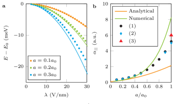
Figure 2: Stark shift and polarizability of the one dimensional H${}_{2}^{+}$ ion. In panel a the Stark shift, $E-E_{0},$ as function of the electrostatic field strength is depicted for three different positions of the proton. The solid lines represent the numerical solution; the dots represent the approximate analytical result. A quadratic behavior with the field strength is observed, since higher order field terms are less relevant in the weak field regime we depict. As $a$ increases, the approximation becomes worse, in agreement with the hypothesis of the expansion used. In panel b the static polarizability of the one dimensional H${}_{2}^{+}$ ion computed from Eq. (14) is compared with that from Ref. [37] (1) and Ref. [38] (2). The “experimental” value of $\alpha_{\parallel}$, estimated via the relation $\alpha=(\alpha_{\parallel}+2\alpha_{\perp})/3$, is represented by a red triangle (the value of $\alpha_{\perp}$ was taken from Ref. [38]). The experimental value of $\alpha$ was retrieved from Ref. [39, 40] (3). Also represented is the numerical calculation of the static polarizability obtained from the numerically exact eigenvalues of Eq. (8).

4 Summary

In this work, the ionization rate and Stark shift of the hydrogen molecule ion $\mathrm{H}_{2}^{+}$ in the presence of an external static electric field were studied. From the Stark shift the static polarizability was extracted. To model this system, we introduced a one dimensional Schrödinger equation where the Coulomb interaction between the two protons and the single electron was replaced by a pair of $\delta-$functions.

In the first part of the text, we analyzed the system in the absence of an electric field, studying the existence of its bound states and their respective binding energies. Afterwards, the problem in the presence of a finite electrostatic field was considered. Solving the Schrödinger equation in the three different regions of the system, we were able to write an eigenvalue problem, from which an implicit relation defining the energy of the quasi-bound states was obtained. This energy corresponds to a complex number whose real part gives the central value of the binding energy, which is Stark shifted relative to the zero field case, while the imaginary part is linked to the line-width of the quasi-bound state or, saying it differently, to the ionization rate. To find an approximate analytical expression describing the energy we focused on the weak field and small internuclear distance limit. Considering the leading order terms, we found an expression for the ionization rate in excellent agreement with the exact numerical results, even when the approximate solution was pushed beyond its expected validity. We observed that the ionization rate was very sensitive to the external electrostatic field strength, spanning many orders of magnitude for small changes on the field’s intensity.

The study of the dependence of the ionization rate on the internuclear distance revealed that for large distances this quantity saturates, which is a direct consequence of the dependence of the energy eigenvalue on the same parameter. Although the leading order approximation produced excellent results for the ionization rate, the same did not apply to the real part of the energy. To improve this, higher order terms had to be considered. Doing so allowed us to obtain results for the Stark shift in good agreement with the numerical ones. However, the zero–th order term of the real part of the energy failed to replicate the result in the absence of the electrostatic field. This is easily understood because the exact eigenenergy comes from the solution of a transcendental equation. Therefore, the zero-th order term is the value of the energy for small $a$, which is to be expected given the approximations made. Finally, the static polarizability was computed and compared with data previously published in the literature (for the three-dimensional ion) and a good agreement was found.

References

References

- [1] Linus Pauling.The application of the quantum mechanics to the structure of the hydrogen molecule and hydrogen molecule-ion and to related problems. Chem. Rev., 5(2):173–213, 1928.
- [2] Szczepan Chelkowski, Tao Zuo, and André D Bandrauk. Ionization rates of h 2+ in an intense laser field by numerical integration of the time-dependent schrödinger equation. Phys. Rev. A, 46(9):R5342, 1992.
- [3] R. G. Clark and E. Theal Stewart. A three-parameter wave function for the hydrogen molecule ion. J. Phys. B: At. Mol. Opt. Phys., 2(3):311, 1969.
- [4] N. R. Arista and V. H. Ponce. Variational approximations to the 2p u and 2p u wavefunctions of the hydrogen molecule ion. J. Phys. B: At. Mol. Opt. Phys., 6(3):511, 1973.
- [5] Alexei M Frolov. Structures and properties of the ground states in h like adiabatic ions. J. Phys. B: At. Mol. Opt. Phys., 35(14):L331–L338, 2002.
- [6] Gerald V. Dunne and Christopher S. Gauthier. Simple soluble molecular ionization model. Phys. Rev. A, 69(5):053409, 2004.
- [7] Kuninobu Nagaya and André D Bandrauk. Laser coulomb explosion imaging of linear triatomic molecules. J. Phys. B: Atom., Mol. Opt. Phys., 37(14):2829, 2004.
- [8] Peter Dietrich and Paul B. Corkum. Ionization and dissociation of diatomic molecules in intense infrared laser fields. J. Chem. Phys., 97(5):3187–3198, 1992.
- [9] R. J. Damburg and V. V. Kolosov. A hydrogen atom in a uniform electric field. J. Phys. B: At. Mol. Opt. Phys., 9(18):3149–3157, 1976.
- [10] Rodney Loudon. One-dimensional hydrogen atom. Proc. R. Soc. A, 472(2185):20150534, 2016.
- [11] Rodney Loudon. One-dimensional hydrogen atom. Am. J. Phys, 27(9):649–655, 1959.
- [12] Francisco M. Fernandez and Eduardo A. Castro. Stark effect in a one-dimensional model atom. Am. J. Phys, 53(8):757–760, 1985.
- [13] R. Blümel and U. Smilansky. Microwave ionization of highly excited hydrogen atoms. Zeitschrift für Physik D Atoms, Molecules and Clusters, 6(2):83–105, 1987.
- [14] R. Blümel. Analytical solution of the compressed, one-dimensional delta atom via quadratures and exact, absolutely convergent periodic-orbit expansions. J. Phys. A: Math. Gen., 39(26):8257, 2006.
- [15] François Fillion-Gourdeau, Emmanuel Lorin, and André D Bandrauk. Relativistic stark resonances in a simple exactly soluble model for a diatomic molecule. J. Phys. A: Math. Theor., 45(21):215304, 2012.
- [16] Sourav Dutta, Shreemoyee Ganguly, and Binayak Dutta-Roy. A cartoon in one dimension of the hydrogen molecular ion. Eur. J. Phys., 29(2):235, 2008.
- [17] L. L. Foldy. An interesting exactly soluble one-dimensional hartree problem. Am. J. Phys, 44(12):1192–1196, 1976.
- [18] Guanhua Yao and Shih-I Chu. Strong field effects in above-threshold detachment of a model negative ion. J. Phys. B: Atom., Mol. Opt. Phys., 25(2):363, 1992.
- [19] Lars Drud Nielsen. A simplified quantum mechanical model of diatomic molecules. Am. J. Phys., 46(9):889–892, 1978.
- [20] B. J. Postma. Polarizability of the one-dimensional hydrogen atom with a -function interaction. Am. J. Phys, 52(8):725–730, 1984.
- [21] B. J. Postma. Photoelectric effect for the one-dimensional hydrogen atom with a -function interaction. Am. J. Phys, 53(4):357–360, 1985.
- [22] Andreas Buchleitner and Dominique Delande. Spectral aspects of the microwave ionization of atomic rydberg states. Chaos, Solitons & Fractals, 5(7):1125–1141, 1995.
- [23] I. Richard Lapidus. One-dimensional model of a diatomic ion. Am. J. Phys, 38(7):905–908, 1970.
- [24] Christer Z. Bisgaard and Lars Bojer Madsen. Tunneling ionization of atoms. Am. J. Phys, 72(2):249–254, 2004.
- [25] E. J. Austin. Ionisation of model atoms by intense electromagnetic fields. J. Phys. B: At. Mol. Opt. Phys., 12(24):4045, 1979.
- [26] S Geltman. Short-pulse model-atom studies of ionization in intense laser fields. J. Phys. B: Atom., Mol. Opt. Phys., 27(8):1497, 1994.
- [27] M. Belloni and Richard Wallace Robinett. Quantum mechanical sum rules for two model systems. Am. J. Phys, 76(9):798–806, 2008.
- [28] Thomas Garm Pedersen. Hypergeometric resummation approach to dissociation and stark effect in non-rigid dipolar molecules. J. Phys. B: Atom., Mol. Opt. Phys., 2020.
- [29] Thomas Garm Pedersen. Analytical models of optical response in one-dimensional semiconductors. Phys. Lett. A, 379(30):1785 – 1790, 2015.
- [30] Milton Abramowitz, Irene A Stegun, and Robert H Romer. Handbook of mathematical functions with formulas, graphs, and mathematical tables. American Association of Physics Teachers, 1988.
- [31] Olivier Vallée and Manuel Soares. Airy functions and applications to physics. World Scientific Publishing Company, 2004.
- [32] Hua Li, Jun Wu, Bing-Lu Zhou, Jiong-Ming Zhu, and Zong-Chao Yan. Calculations of energies of the hydrogen molecular ion. Phys. Rev. A, 75:012504, 2007.
- [33] R. P. Bell and D. A. Long. Polarizability and internuclear distance in the hydrogen molecule and molecule-ion. Proc. R. Soc. Lond., 203(1074):364, 1950.
- [34] C. S. Lai and B. Suen. Ionization energies of the hydrogen molecule ion in strong magnetic fields. Can. J. Phys., 55(7-8):609–614, 1977.
- [35] G. N. Gibson, M. Li, C. Guo, and J. Neira. Strong-field dissociation and ionization of h 2+ using ultrashort laser pulses. Phys. Rev. Lett., 79(11):2022, 1997.
- [36] Liang-You Peng, JF McCann, Daniel Dundas, KT Taylor, and ID Williams. A discrete time-dependent method for metastable atoms and molecules in intense fields. J. Chem. Phys., 120(21):10046–10055, 2004.
- [37] R. P. McEachran, Sharon Smith, and M. Cohen. The dipole polarizability of the hydrogen molecular ion: A variational two-center calculation. Can. J. Chem., 52(20):3463–3467, 1974.
- [38] Ts. Tsogbayar and Kh. Namsrai. The dipole polarizability of the hydrogen molecular ion. AIP Conf. Proc., 1109(1):122–124, 2009.
- [39] W. G. Sturrus, E. A. Hessels, P. W. Arcuni, and S. R. Lundeen. Microwave spectroscopy of the high-l rydberg states (=0, r=1) n=10 g, h, i, and k. Phys. Rev. A, 44:3032–3053, 1991.
- [40] P. L. Jacobson, D. S. Fisher, C. W. Fehrenbach, W. G. Sturrus, and S. R. Lundeen. Determination of the dipole polarizabilities of and by microwave spectroscopy of high- rydberg states of and . Phys. Rev. A, 56:R4361–R4364, 1997.