Residual Generation Using Physically-Based Grey-Box Recurrent Neural Networks For Engine Fault Diagnosis

Abstract

Data-driven fault diagnosis is complicated by unknown fault classes and limited training data from different fault realizations. In these situations, conventional multi-class classification approaches are not suitable for fault diagnosis. One solution is the use of anomaly classifiers that are trained using only nominal data. Anomaly classifiers can be used to detect when a fault occurs but give little information about its root cause. Hybrid fault diagnosis methods combining physically-based models and available training data have shown promising results to improve fault classification performance and identify unknown fault classes. Residual generation using grey-box recurrent neural networks can be used for anomaly classification where physical insights about the monitored system are incorporated into the design of the machine learning algorithm. In this work, an automated residual design is developed using a bipartite graph representation of the system model to design grey-box recurrent neural networks and evaluated using a real industrial case study. Data from an internal combustion engine test bench is used to illustrate the potentials of combining machine learning and model-based fault diagnosis techniques.

I Introduction

Fault diagnosis of industrial systems is about monitoring the system health including detection of occurring faults and identifying their root cause. One of the main principles of fault diagnosis is to detect inconsistencies between sensor data from the monitored system and predictions computed based on a model of the system behavior. Two common approaches to compute predictions are based on physically-based or data-driven models.

Model-based diagnosis relies on physically-based models that are derived based on first principle physics. Model parameters can be derived from physical properties of the system to be monitored, referred to as white-box modeling, or estimated from data, referred to as grey-box modeling [1].

Data-driven models rely on representative training data to select and train a general-purpose model structure that best captures the multi-variate information in training data. The parameters and model structure of data-driven models do seldom have a physical interpretation with respect to the modeled system and are therefore referred to as black-box models [1].

Developing sufficiently accurate physically-based models for residual generation is a time-consuming process and requires expert knowledge about the system to be modeled, especially for complex or large-scale systems. This have motivated the use of data-driven modeling and machine learning to design diagnosis systems [2]. However, collecting representative training data for fault diagnosis applications is a difficult task. Many different types of faults could occur in the system and each type of fault can have many different realizations due to varying operating conditions and fault magnitudes [3]. Certain fault types can be difficult to collect data from and there could be faults that are not considered when designing the diagnosis system, resulting in imbalanced training data and unknown fault classes that are not represented in training data, which complicates conventional closed set multi-class data-driven fault classification [4, 5].

Instead of using data-driven models with a general-purpose model structure, there are benefits when selecting a model structure that captures the physical relationship between input and output variables [6]. It is possible to reduce the model parameter space and the number of input variables by identifying which variables have sufficient information for regression, i.e. to capture the behavior of a predicted variable. If the model structure is given, less training data are needed to model the remaining non-linearities which also reduces the risk of overfit. A physically-based model structure also improves model interpretability since different parts of the model correspond to different system components [7]. Another potential benefit is to achieve similar fault isolation capabilities as model-based residuals [3]. By including physical insights in data-driven anomaly classifiers it is possible to identify the root cause of unknown fault classes, for example, by mapping triggering residuals to components that are modeled in each residual generator [8].

Recurrent neural networks (RNN) are powerful black-box models able to capture the behavior of non-linear dynamic systems [9]. Neural networks have a flexible model structure making them applicable in many different applications. However, a general drawback of general-purpose models, such as neural networks, is that they can contain lots of parameters to fit in order to model the behavior of the system which requires a significant amount of training data to avoid overfitting [10]. Utilizing physical insights about the system to be monitored can help select a neural network model structure that resembles the physical system. Designing grey-box RNN based on physical models for residual generation has been proposed in, e.g., [11]. In [8], a simulation study indicates that grey-box neural networks can identify the root cause of unknown fault classes. However, to make this useful for fault diagnosis in industrial systems, it is relevant to investigate how to systematically design and train grey-box RNN to achieve certain fault classification properties.

II Problem Statement

Designing grey-box RNN for residual generation is a promising approach to combine physical insights about the system to be monitored and machine learning for fault diagnosis. Since faults are rare events, it is likely that training data are imbalanced and consists mainly of data from fault-free system operation. Residual generators are anomaly classifiers meaning that training only requires fault-free data to detect abnormal system behavior caused by faults. By designing different residual generators that are sensitive to different faults, it is possible to isolate faults by analyzing the resulting fault patterns.

In this work, the objective is to develop a diagnosis system combining model-based and machine learning methods applied to an internal combustion engine test bench. A set of data-driven residual generators are designed using grey-box RNN and trained using only nominal training data. An automated design process is developed where the RNN models are generated based on a structural model representing the physical insights about the system model structure.

Structural models are bi-partite graphs that represent the qualitative relationship between different model variables and can be used even though the analytical relationship is not completely known [12]. The usefulness of structural models for fault diagnosis analysis and diagnosis system design have been shown in, e.g., [13, 14], and can be used for, for example, fault isolability analysis, residual generation, and sensor placement [15].

To evaluate the proposed method, an internal combustion engine test bench is used as a case study. Both training and validation data are collected from the test bench when the engine is working in transient operation. A structural model of the air path through the engine is used to represent the available model information that is used to design different grey-box RNN modeling different parts of the engine.

III Related Research

Data-driven classification that considers both known and unknown classes is referred to as open set classification [16]. Different approaches to open set classification have been proposed, see e.g. [3] and [17]. Even though these mentioned work are able to identify when data belong to unknown fault classes, it is not trivial how to identify the true class label. In [3], model-based residuals are used to compute fault hypotheses based on the fault sensitivity of each residual generator and a set of anomaly classifiers are used to rank the known fault classes.

Neural networks have been used for fault diagnosis in many different applications [18]. Feature extraction using neural networks is proposed in, e.g. [19]. In [20], neural networks are used to develop a grey-box simulation model of an HCCI engine. In [21], neural networks and genetic programming are used for non-linear residual design for fault diagnosis of an industrial valve actuator. A hybrid system identification approach combining model-based and neural networks is proposed in [22] where a weighted prediction is computed from the model-based and data-driven models. In [23], neural networks are used for fault diagnosis of a wind turbine.

The benefits of bridging and combining physically-based fault diagnosis methods and machine learning have been discussed in, e.g., [24]. The connections between different neural network structures and ordinary differential equations have been analyzed in, e.g. [25] and [26]. Including physical insights about the system to design grey-box neural networks have been proposed in previous works, such as [11, 27] and [28]. In [29], hamiltonian dynamics are incorporated in the neural network structure. Grey-box RNN, based on state-space neural networks [30], are proposed in [11] for residual generation to perform fault diagnosis of an evaporator in a sugar beet factory. With respect to previous work, an automated design process of grey-box RNN for residual generation is developed here combining physically-based structural models and deep learning techniques applied to an automotive case study.

IV Artificial Neural Networks

An artificial neural network models the relationship between a set of inputs $u\in\mathbb{R}^{n_{u}}$ and outputs $y\in\mathbb{R}^{n_{y}}$ using a computational graph, as illustrated in Fig. 1, where each node represents a non-linear operation on the inputs to the node, $x_{in}$, usually in the form:

$$x_{out}=g(a^{T}x_{in}+b)$$ (1)

where $g(\cdot)$ is a non-linear function, called an activation function, $a$ is vector of weights, and $b$ is a bias term. Some common activation functions are the rectified linear unit (ReLU)

$$g(\xi)=\max\left(0,\xi\right)$$

and different sigmoid functions, such as the logistic function or arc tangent function [10].

Figure 1: An example of an artificial neural network with $k$ inputs and one output.

Neural networks are commonly designed such that the nodes are organized in different layers where the inputs to each node are the output of nodes in the previous layer and the nodes in the same layers have the same activation function. The first layer is referred to as the input layer, where data is fed into the neural network. The last layer is the output layer, which returns the output from the neural network model, and the in-between layers are referred to as hidden layers. The number of layers denotes the depth and the maximum number of nodes in any layer the width of the neural network.

Training of neural networks is performed by defining a cost function, e.g. mean square error $\sum(y-\hat{y})^{2}$ for regression problems, and updating the model parameters by computing gradients using back-propagation and automatic differentiation [10]. Training neural networks is a non-linear optimization problem that can be computationally demanding since these models can have a large amount of parameters to fit. Different optimization solvers, regularization techniques, and training strategies have been proposed to improve learning rate, avoid overfit and reduce the risk of getting stuck in bad local minima [10].

IV-A Recurrent Neural Networks

Recurrent neural networks are used to model dynamic systems and time-series data. Internal states are modeled by in the neural network by duplicating the network for each time instance and add connections in some nodes between different time steps, similar as state variables in a state-space model [10].

V Model-based diagnosis and structural modeling

Model-based diagnosis uses physically-based models of the system to be monitored to compute residuals $r$ that compare model predictions $\hat{y}$ and sensor data $y$ to detect inconsistencies, as illustrated in Fig. 2. An advantage of model-based diagnosis, with respect to data-driven methods, is that it is possible to identify the root cause of unknown faults by designing residual generators where the effects of certain faults are decoupled. One efficient approach to analyze large-scale non-linear models is called structural methods, see for example [14]. In this work, structural methods will be used to find and generate neural network models for residual generation. Here, an introduction to model-based diagnosis and structural models is presented.

Figure 2: An example of a residual $r_{t}$ comparing measurements from the system $y_{t}$ with model predictions $\hat{y}_{t}$.

V-A Fault detection and isolation

A residual generator models the nominal system behavior where a significant deviation in the residual output implies that a fault has occurred. Thus, a residual can be interpreted as an anomaly classifier modeling data from the fault-free class [8].

By designing residual generators based on different sub-models, it is possible to decouple the effects of different faults on the residual outputs [3].

Definition 1

A residual $r_{k}$ is said to be (ideally) sensitive to a fault $f_{i}$ if $f_{i}\neq 0$ implies that $r_{k}\neq 0$.

If a residual $r_{k}$ is not sensitive to a fault $f_{i}$, the fault is said to be decoupled in that residual.

Even though the set of residual generators is a set of anomaly classifiers, their fault sensitivities can be used to identify the root cause by analyzing their fault sensitivities.

Definition 2

A fault $f_{i}$ is isolable from fault $f_{j}$ if there is a residual $r_{k}$ that is sensitive to $f_{i}$ but not $f_{j}$.

The fault sensitivities of a set of residuals can be summarized in a fault signature matrix where an X in position $(i,j)$ means that residual $r_{i}$ is sensitive to fault $f_{j}$. By analyzing the fault sensitivities of the set of residuals that are deviating from their nominal behavior, a set of fault hypotheses, also called diagnosis candidates, can be computed [31].

V-B Change detection

One of the simplest methods to detect a change in the nominal residual output is to compare it with a threshold $r_{t}-J>0$ that is tuned to not exceed a certain false alarm rate. This approach is not suitable to detect small faults while having to fulfill a low false alarm rate. One solution is to use a CUMulative SUm (CUSUM) test [32]:

$$T_{t}=\max\left(0,T_{t-1}+r_{t}-\nu\right),\quad T_{0}=0$$ (2)

where $\nu$ is a tuning parameter. The CUSUM test (2) integrates the impact of the fault on the residual output (exceeding the parameter $\nu$) over time and a fault is detected by tuning a threshold $J$ such that $T_{t}-J>0$. This allows for detection of smaller faults without increasing the risk of false alarms by allowing a longer time before detection.

V-C Structural models

Structural analysis can be used to analyze fault diagnosis properties of complex non-linear dynamic systems and systematic design of diagnosis systems [15]. A structural model $\mathcal{M}=(\mathcal{E},\mathcal{X})$ is a bi-partite graph describing the relationship between model equations $\mathcal{E}=\{e_{1},e_{2},...\}$ and variables $\mathcal{X}=\{x_{1},x_{2},...\}$, i.e. which variables are included in each model equation. The structural model can be represented using an incidence matrix where an X in row $(i,j)$ mean that variable $x_{j}$ is included in equation $e_{i}$. Model variables are partitioned into unknown variables, known variables, and fault signals that are used to model how different faults are affecting the system.

The rows and columns of the incidence matrix can be reorganized using the Dulmage-Mendelsohn (DM) decomposition [33] to analyze the structural redundancy properties of the system [15]. The DM decomposition partitions a structural model into an under-determined part $\mathcal{M}^{-}$, an exactly determined part $\mathcal{M}^{0}$, and an over-determined part $\mathcal{M}^{+}$ as illustrated in Fig. 3. The over-determined part of the model has more equations than unknown variables and describes the redundant part of the model that can be monitored using residual generators [14]. The degree of structural redundancy of a model $\mathcal{M}$ is defined as [14]:

$$\varphi(\mathcal{M})=|\mathcal{E}^{+}|-|\mathcal{X}^{+}|$$ (3)

where $|\cdot|$ denotes set cardinality.

Figure 3: Dulmage-Mendelsohn decomposition of a model $\mathcal{M}=\left(\mathcal{E},\mathcal{X}\right)$.

A fault that enters the system somewhere modeled in the over-determined part, i.e. $e_{f_{i}}\in\mathcal{M}^{+}$ where $e_{f_{i}}$ denotes the model equation modeling where the fault $f_{i}$ manifests in the system, is said to be structurally detectable. Similarly, a fault $f_{i}$ is said to be structurally isolable from fault $f_{j}$ if $e_{f_{i}}\in\left(\mathcal{M}\setminus e_{f_{j}}\right)^{+}$, i.e. fault $f_{i}$ is structurally detectable if $e_{f_{i}}$ is still in the over-determined part when the equation $e_{f_{j}}$ is removed from the model. In principle, structural fault detectability and isolability depend on if it is possible to design a residual generator modeling the part of the system where the fault $f_{i}$ occurs or not.

Different residual candidates can be found by analyzing different subsets of the over-determined part of the model $\mathcal{M}^{+}$ that are still over-determined. By systematically removing equations from the over-determined part and analyzing the remaining over-determined part it is possible to find all combinations of redundant equation sets, called Partially Structurally Over-determined (PSO) sets [14].

Definition 3

A structural model $\mathcal{M}$ is called a Partially Structurally Over-determined set if $\mathcal{M}=\mathcal{M}^{+}$.

A special type of PSO set have degree of redundancy one, i.e. PSO sets where no subset have redundancy, called Minimally Structurally Over-determined sets [14].

Definition 4

A PSO set $\mathcal{M}=\mathcal{M}^{+}$ is called a Minimally Structurally Over-determined (MSO) set if $\left(\mathcal{M}\setminus e_{k}\right)^{+}=\emptyset$ for all $e_{k}\in\mathcal{M}$.

The MSO sets represent the minimal redundant equation sets that can be used for residual generation. MSO sets are interesting from a fault isolation perspective since they model a minimal part of the system that can be monitored.

V-D Designing Residual Generators Using Computational Graphs

If one equation is removed from an MSO set, the remaining set is exactly determined, meaning that there is an equal amount of unknown variables and equations. A matching algorithm can be used to find how to compute all unknown variables in the exactly determined set [34]. When all unknown variables have been computed in the exactly determined set, the redundant equation can be used as a residual equation.

The output from the matching algorithm describing the order of computing the unknown variables can be represented as a computational graph. A computational graph is a directed graph where nodes either denote a variable or a function and edges show how the output of each node are fed as input to other nodes, which is illustrated in Fig. 1. The order of how the state variables are computed in the computational graph will affect its causality. If all the states are computed by integrating their derivatives the computational graph is said to have integral causality. If the state variable is computed and then differentiated to get its derivative the computational graph is said to have derivative causality. If there are both states that are integrated and differentiated the computational graph is said to have mixed causality [34]. Computational graphs of different causalities are illustrated in the following example:

Example 1

Consider the following MSO set

$$e_{1}: \dot{x}_{1} =g_{1}(u) e_{4}: \dot{x}_{1} =\frac{dx_{1}}{dt}$$ (4)

$$e_{2}: \dot{x}_{2} =g_{2}(x_{1}) e_{5}: \dot{x}_{2} =\frac{dx_{2}}{dt}$$

$$e_{3}: y =x_{2}$$

where $g_{1}$ and $g_{2}$ are invertible. When each of the equations $e_{1}$, $e_{2}$, and $e3$, are selected as residual equation, the resulting computational graphs are given in Fig. 4. The corresponding computational graph when $e_{1}$ is used as residual equation has derivative causality, when $e_{2}$ is used it has mixed causality, and when $e_{3}$ is used it has integral causality.

Figure 4: An illustration of three different computational graphs with different causalities using the same MSO set (4) but different residual equations.

The structure of the computational graph illustrate the structural relationships between input and output variables and state variables even though the analytical relationships are unknown. This can give useful information to include physical insights in the model structure of a recurrent neural network.

VI Design of RNN Using Structural Models

Discrete-time non-linear state-space models can be modeled using RNN. Here, computational graphs are derived from MSO sets with integral causality. These MSO sets have a DAE index equal to zero or one which means that they can be written in state-space form [35], i.e.

$$\dot{x} =\bar{g}(x,u)$$ (5)

$$r =y-h(x,u)$$

where $x$ are state variables, $u$ are known inputs, $y$ is the signal to predict, and $\bar{g}=\left(g_{1},g_{2},\ldots\right)^{T}$. Note that $u$ could include both actuator and sensor signals depending on the computational graph. The arguments to each function $g_{i}(x,u):\mathcal{R}^{|x|+|u|}\rightarrow\mathcal{R}$ are determined by backtracking from each corresponding state derivative $\dot{x}_{i}$ in the computational graph until a state variable $x$ or an input signal $u$ is found which give the arguments to each function $g_{i}(x,u)$. Similarly, the arguments to the function $h(x,u):\mathcal{R}^{|x|+|u|}\rightarrow\mathcal{R}$ are determined by back-tracking from the residual equation in the computation graph until a state variable or and input signal is found.

When the arguments have been found, the time-continuous state-space model (5) can be formulated in discrete-time, using Euler forward, as

$$x_{t+1} =x_{t}+T\,\bar{g}(x_{t},u_{t})$$ (6)

$$r_{t} =y_{t}-h(x_{t},u_{t})$$

where $T$ is the sampling time.

Once the structure of the discrete-time state space model is determined, an RNN is generated with the same structure as the model (6) [13]. The non-linear functions $g_{i}$ and $h$ are modeled using a general fully-connected neural network structure with a scalar output and the input vector corresponds to the arguments in (6) derived from the computational graph, similar to the neural network shown in Fig. 1.

VII Internal Combustion Engine Case Study

As a case study, the air path through an internal combustion engine is considered which is illustrated in Fig. 5. Both nominal and faulty data have been collected from a test bench during transient operation. The engine is an interesting case study since the system is dynamic and non-linear and it is used for both transients and stationary operating conditions. Another complicating aspect from a fault diagnosis perspective is the coupling between the intake and exhaust flow through the turbine and compressor. This results in that a fault somewhere in the system, including sensor faults, will not have an isolated impact in that component but is likely to affect the behavior, and thus the sensor outputs, in other parts of the system as well.

Figure 5: A schematic of the model of the air flow through the model. This figure is used with permission from [36].

VII-A Model

The structural model used in this case study is based on a mathematical mean value engine model that has been used in previous works for model-based residual generation, see for example [3, 37]. The mathematical model structure is similar to the model described in [38], which is based on six control volumes and mass and energy flows given by restrictions, see Fig. 5.

A structural representation of the engine model, used in this work, is shown in Fig. 6 where a mark in position $(i,j)$ denotes that the variable $x_{j}$ is included in equation $e_{i}$. The model variables are organized in unknown variables $\mathcal{X}$ (including state variables), known variables $\mathcal{Z}$, including known actuators and sensor outputs, and fault signals $\mathcal{F}$. To state the relation between state variables and their derivatives in the structural model, state variables are marked as I and their derivatives as D in the figure [15]. The structural model has 94 equations, 90 unknown variables, including 14 state variables and their derivatives, 11 fault variables, and 10 known variables.

Figure 6: A structural model of the internal combustion engine.

A Dulmage-Mendelsohn decomposition of the structural model in Fig. 5 is shown in Fig. 7. The over-determine part is shown in the blue square. The variables located in the upper left part of the figure belong to the exactly determined part of the model.

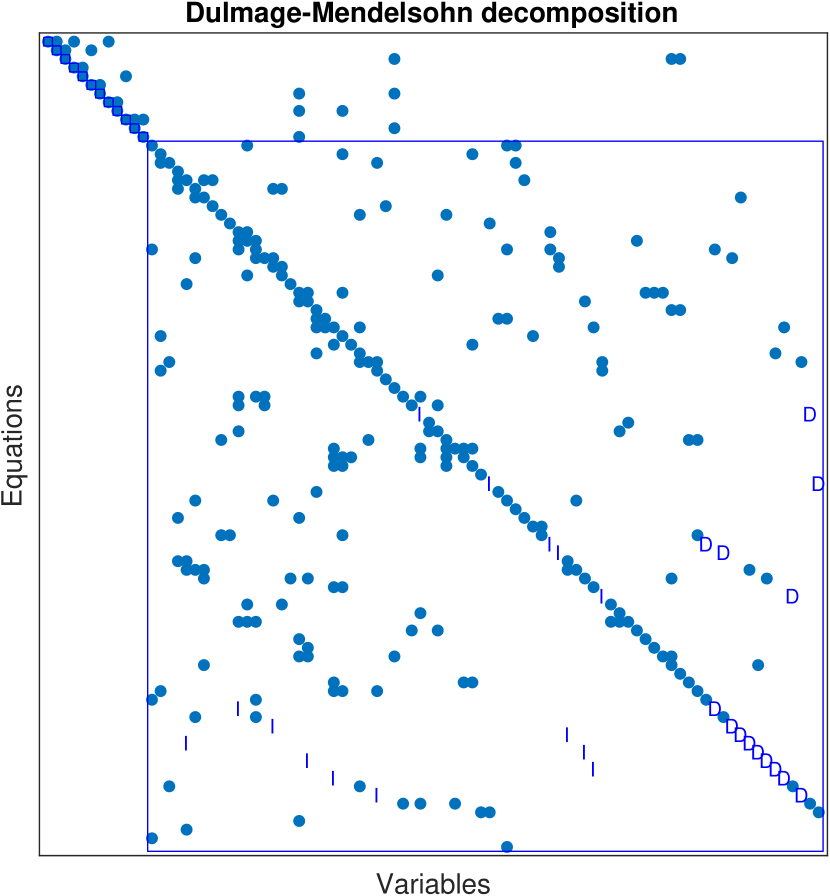
Figure 7: Dulmage-Mendelsohn decomposition of engine model. The blue square represents the over-determined part of the model. State variables and their derivatives are denoted I and D in the matrix.

VII-B Data

Operational data for training and validation have been collected from an engine test bench during transient operation. To cover a large range of operating conditions, data are collected from the engine when it follows the Worldwide Harmonized Light Vehicles Test Procedure (WLTP) cycle, see Fig. 8.

Figure 8: Training data have been collected when the engine has been operated to follow the WLTP cycle.

The set of available sensors in the engine corresponds to a standard setup used in a conventional car. A list of which sensor data are collected in each data set is summarized in Table I and some examples of collected data from nominal and faulty operation (fault in sensor $y_{pim}$) are shown in Fig. 9. Data are downsampled from 1 kHz to 20 Hz to reduce the computational complexity while still capturing the dynamics of the engine. Each signal is normalized such that nominal signal output is in the range of about [0, 1].

TABLE I: A summary of actuator and sensor signals collected from the engine.

Signal	Description
$u_{wg}$	Wastegate reference signal
$u_{mf}$	Estimated total fuel mass flow in all cylinders
$y_{pic}$	Measured pressure at intercooler
$y_{pim}$	Measured pressure at intake manifold
$y_{Tic}$	Measured temperature at intercooler
$y_{waf}$	Measured air mass flow through air filter
$y_{\omega}$	Measured engine speed
$y_{xpos}$	Measured throttle angle
$y_{pamb}$	Measured ambient pressure
$y_{Tamb}$	Measured ambient temperature

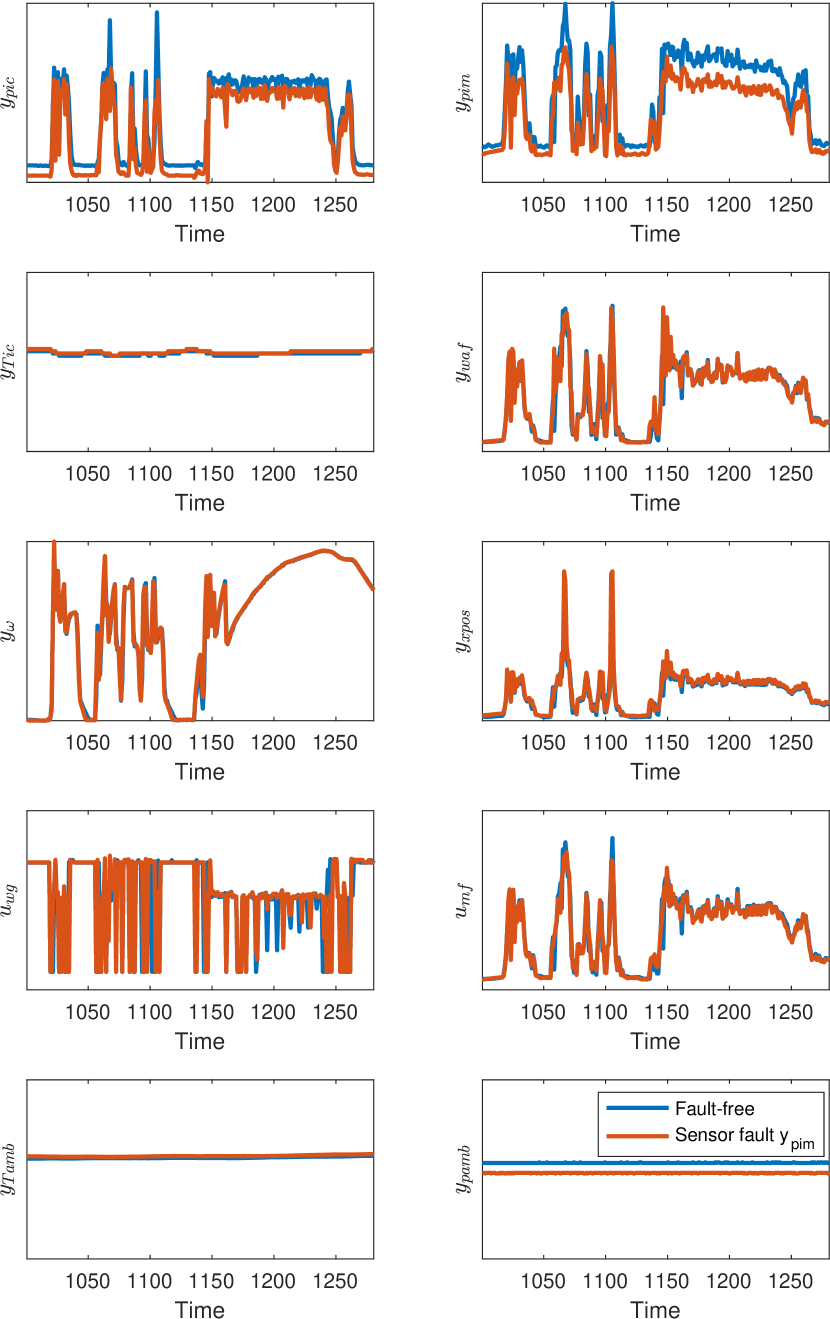
Figure 9: Example of engine data from fault-free and faulty operation when there is a fault in sensor $y_{pim}$. Note that the sensor fault affects the system behavior and is visible in other signals as well, e.g. $y_{pic}$.

Experimental data have been collected from different sensor fault scenarios and leakages, see Table II. Multiplicative sensor faults of different magnitudes have been injected by modifying the corresponding signal directly in the engine control unit during operation. This is illustrated in Fig. 9 comparing engine sensor data from nominal case and scenario with fault in sensor measuring intake manifold pressure. The sensor fault has impact on the general system operation and is affecting other measured states as well.

TABLE II: A summary of fault scenarios collected from engine test bench.

Fault	Description
$f^{Wth}$	Leakage before throttle
$f^{ypic}$	Intermittent fault in sensor measuring pressure at intercooler
$f^{ypim}$	Intermittent fault in sensor measuring intake manifold pressure
$f^{ywaf}$	Intermittent fault in sensor measuring air flow through air filter

VIII Experiments

A set of grey-box RNN is generated based on MSO sets derived from the structural model. The RNN model structures are designed using computational graphs with integral causality and where the residual equation is a sensor equation, i.e. $r_{t}=y_{t}-\hat{y}_{t}$. The steps of the design procedure are summarized in Fig. 10. Then, the generated grey-box RNN are evaluated as residual generators using collected data from the engine test bench. With a slight abuse of notation, the MSO set index MSO_i will be used in the text when referring to the generated grey-box RNN and residual generator.

Figure 10: The design procedure of generating residual generators using grey-box RNN from a structural model.

VIII-A Residual Generation

First, a set of MSO sets is computed based on the structural model using the Fault Diagnosis Toolbox [15] in Matlab. A causality analysis is performed on each of the 144 candidate MSO sets to identify which MSO sets that can be used to generate computational graphs with integral causality, resulting in 17 sets. Out of these 17 MSO sets it is possible to generate 21 different computational graphs with integral causality. The grey-box RNN and resulting residual generators will be referred to in the text based on which of the 144 original MSO sets they are generated from.

Only the computational graphs where one of the sensors $y_{pim}$, $y_{pic}$, or $y_{waf}$ are used as residual equation, are used to generate grey-box recurrent neural networks to be used in this case study. The other candidates have residual equations based on sensors measuring slowly varying states, such as temperatures, as shown in Fig. 9. These sensor signals do not show sufficient excitation in training data and are, therefore, not used as residual equations.

The model support of each MSO set that is used for generating computational graphs in this study, is shown in Fig. 11. A mark in position $(i,j)$ means that equation $e_{j}$ is included in MSO set $i$. It is visible that the MSO sets share most of the equations in this case study. This can be explained by that the engine has few sensors and is strongly coupled meaning that a large part of the model is needed to achieve redundancy. Note that equations $e_{47}$-$e_{56}$ are not included in any MSO set. These equations corresponds to the equations not included in the over-determined part of the model $\mathcal{M}^{+}$ in Fig. 7.

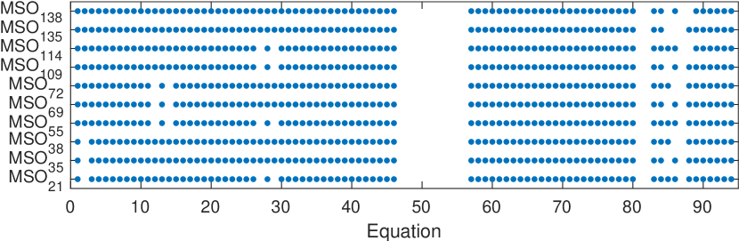
Figure 11: The model support of each evaluated MSO set.

The generated computational graphs are then used to automatically generate a set of grey-box RNN. An incidence matrix used to derive the matching of MSO₂₇ is shown in Fig. 12 going down-to-up. The incidence matrix represents a bi-partite graph and the matching is interpreted as each variable in the diagonal can be computed based on the variables marked on the same row. Rows with I on the diagonal denotes computation of state variables by integrating their derivatives. The result is a computational graph representing the state-space model which only depends on known variables and state variables (5).

The grey-box RNN, generated based on the computational graph derived from Fig. 12, is shown in Fig. 13. The non-linear functions $g_{i}(\cdot)$ and $h(\cdot)$ are modeled using a three layer neural network structure, with 256 nodes in each hidden layer, and a scalar output, similar as the one illustrated in Fig. 1. The dimension of the input layer is determined from the computational graph. Different activation functions have been evaluated where ReLU gave the overall best results and is therefore used in all grey-box RNN generated in this case study.

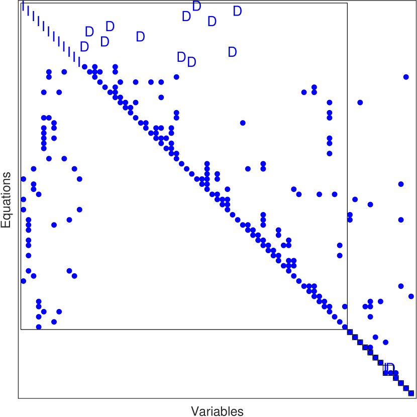
Figure 12: Matching of MSO₂₇ used to derive computational graph. Starting from the lowest row, each unknown variable on the diagonal can be computed based on previously computed variables are states.

Figure 13: A schematic of the grey-box RNN estimating the output $\hat{y}_{pic,t}$ based on MSO₂₇ where each function $g_{i}(\cdot):\mathbb{R}^{n_{i}}\rightarrow\mathbb{R}$ and $h(\cdot):\mathbb{R}^{n_{h}}\rightarrow\mathbb{R}$ is modeled using a static neural network.

VIII-B Training

Each neural network is trained using only fault-free data where the time series data are partitioned into a set of 19 equally sized batches of 600 samples covering different operating conditions. Training is done in Python, using PyTorch [39], by minimizing the mean square prediction error $\frac{1}{N}\sum_{t=1}^{N}(y_{t}-\hat{y}_{t})^{2}$. The initial values of the state variables are unknown and are set to some reasonable reference value that is used for all batches. The optimization algorithm ADAM [40] is run for 2000 epochs with an adaptive learning rate starting at $5*10^{-4}$ which is reduced every 10th epoch by $3\%$. The loss after each epoch is shown in Fig. 14 for grey-box RNN predicting $\hat{y}_{pic}$ and in Fig. 15 for grey-box RNN predicting $\hat{y}_{pim}$.

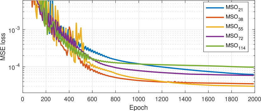
Figure 14: Loss after each epoch when training neural networks predicting $y_{pic}$.

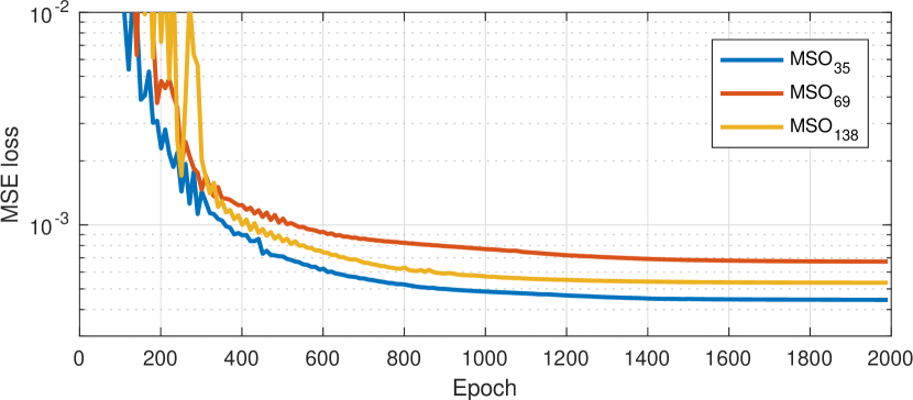
Figure 15: Loss after each epoch when training neural networks predicting $y_{pim}$.

Model prediction of three grey-box RNN set are shown in Fig. 16, each one predicting one of the different sensor outputs. It is visible that the different grey-box RNN capture the general dynamic behavior of the different sensor signals. Similar prediction performance is achieved for the remaining grey-box RNN. The residual outputs have a small bias in the datasets that are likely to be caused by incorrect initial conditions of the state variables. If it is assumed that there are no faults when a scenario begins, the residual bias can be removed by subtracting the median computed from a short time interval in the beginning of the residual output for each dataset.

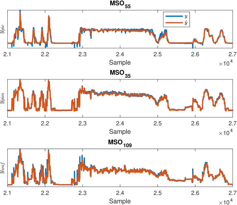
Figure 16: Evaluation of prediction performance of three grey-box RNN.

VIII-C Fault Diagnosis Performance

Fault detection performance is evaluated for the set of residual generators using data from different fault realizations. Figure 17 shows four of the residual generators where their outputs are plotted as histograms comparing different fault scenarios and nominal operation. The sensor fault scenarios are multiplicative of magnitude $f=-20\%$, i.e. $y=(1+f)x$. The sensor that is predicted in each residual generator is highlighted in gray in Fig. 17. Note that faults in predicted sensor signals have a clear impact on the residual outputs while detection performance for other faults is varying between different residuals.

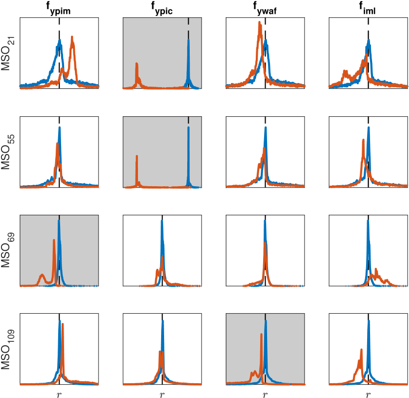
Figure 17: Histograms of residual outputs during different fault scenarios. The blue curve represents the residual output during fault-free case and the red curve when a fault is present. Plots are highlighted when the sensor fault is affecting the sensor signal that predicted by the grey-box RNN used in the residual generator.

To further analyze detection performance, a Receiver Operating Characteristics (ROC) curve is computed for different fault magnitudes. Figure 18 shows detection performance for a couple of different of residuals by evaluating the area under the curve (AUC) is plotted as function of fault size. Multiplicative sensor faults are evaluated for magnitudes in the range [-20%, 20%]. Since $\text{AUC}=0.5$ corresponds to that the histograms from nominal and fault case are identical, the plotted AUC curves in Fig. 18 are normalized as $2*(\text{AUC}-0.5)$. Faults affecting the predicted sensor signal in each residual are highlighted in gray. It is visible that these faults are easiest to detect by each residual. Some faults have little or no impact on the residual outputs, e.g. the residuals based on MSO₂₁, MSO₅₅, and MSO₆₉ are not sensitive to fault $f_{ywaf}$ since AUC is almost zero for all fault magnitudes.

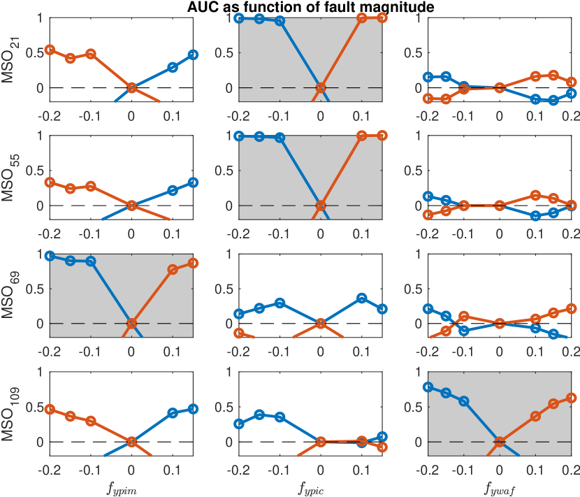
Figure 18: ROC area under curve as function of fault size. The blue curve represents the area under the ROC curve for a test $r>J$ and the red curve a test $-r>J$ when varying the threshold $J$.

Even though detection performance varies between the different residual generators, the multi-variate fault patterns are still useful for fault classification. A t-distributed Stochastic Nearest Embedding (t-SNE) plot is generated to visualize how well the set of residual generators are able to separate data from different faults classes. The t-SNE plot is a non-linear projection of high-dimensional data to a lower-dimensional space where pair-wise similarities between samples are preserved [41]. Residual outputs from the four residual generators in Fig. 17 using data from all different fault classes and fault realizations are used as input to the t-SNE algorithm. Data is then down-sampled to improve visualization. It is visible in the figure that data from the different faults are not overlapping with the fault-free data points, indicating that all faults are detectable. It is also visible that most faults are distinguishable from each other except that data from a leakage in the intake manifold $f_{iml}$ are overlapping with data from sensor fault $f_{ypim}$ which is reasonable since they are located in the same part of the engine.

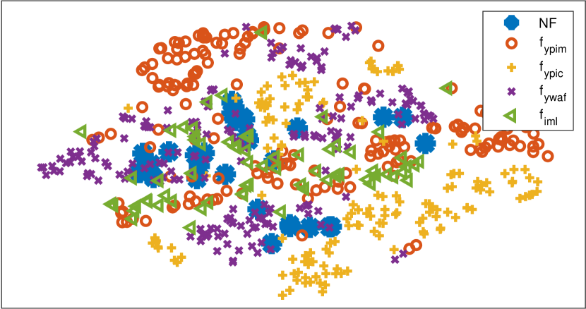
Figure 19: t-SNE plot of residual output data from the four residuals in Fig. 17 evaluated on different fault classes. Data is down-sampled to improve visualization.

VIII-D Prediction Error Estimation Using Ensemble Neural Networks

Since training of neural networks is a non-linear optimization problem, it is beneficial to train multiple instances of each RNN and then select the model with best accuracy to reduce the risk of getting stuck in a bad local minima. Another way of using the multiple trained instances is to estimate confidence intervals.

Results in [42] indicate that using random initialization of the parameters when training each neural network is sufficient to get a set of uncorrelated models. The eight trained instances are combined into an ensemble neural network prediction model. The ensemble model prediction is computed based on the average predicted value for all models and a confidence interval can be estimated by computing the variance over all predictions in each time instance. Figure 20 shows the mean and confidence intervals computed as 3*std based on the original predictions. The figure shows that the confidence intervals varies over time and, in general, increase during transients and are smaller during stationary operation.

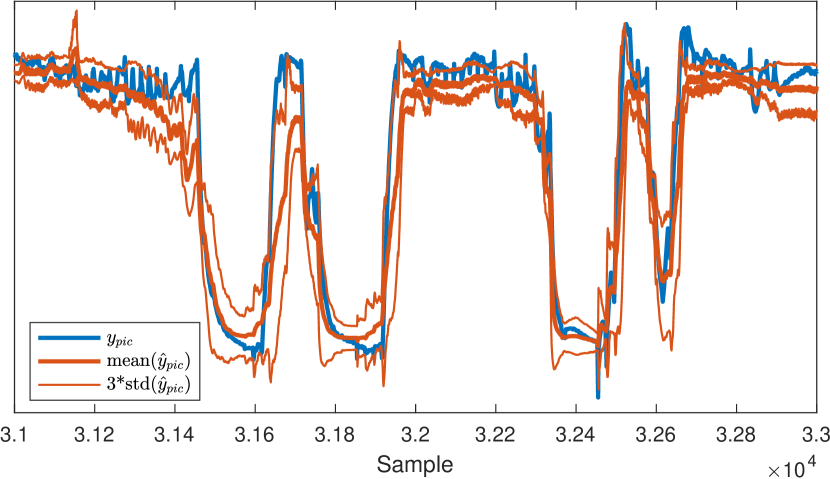
Figure 20: Ensemble prediction of sensor output $y_{pic}$ using eight trained neural networks based on MSO₅₅. The plot show mean prediction and 3*std confidence intervals.

VIII-E Change Detection Using CUSUM Tests

The detection performance in Fig. 18 is evaluated sample-by-sample. However, faults are usually present during a longer time period and, therefore, it is beneficial to take residual time-series information into consideration during the fault detection process. To improve classification performance, a set of CUSUM tests (2) are constructed based on the residual outputs. CUSUM tests are used in, e.g., model-based diagnosis to improve fault detection performance of small faults by allowing a longer time to detection without increasing the risk false-alarms. For each residual, two CUSUM tests are created: one to detect positive change and one to detect negative change:

$$T^{+}_{t} =\max\left(0,T^{+}_{t-1}+r_{t}-\nu^{+}\right)$$ (7)

$$T^{-}_{t} =\max\left(0,T^{-}_{t-1}-r_{t}-\nu^{-}\right)$$

The parameters $\nu^{+}$ and $\nu^{-}$ in (2) are tuned for each test using fault-free data to fulfill requirements regarding false alarm rate. The results in Fig. 21 and Fig. 22 show the CUSUM tests based on residual generators MSO₅₅ and MSO₆₉ respectively. The CUSUM tests are small in the nominal case and increases over time when the fault is present. Note that even though the AUC curve in Fig. 18 is small, for example detection of fault $f_{ypim}$ using MSO₅₅, the CUSUM test accumulates fault information over time which improves detection performance as shown in Fig. 21.

Figure 21: Fault detection using CUSUM tests based on residual generator MSO₅₅. The blue curve shows $T^{+}_{t}$ and the red curve $T^{-}_{t}$. The dashed lines show when the faults occur in each scenario.

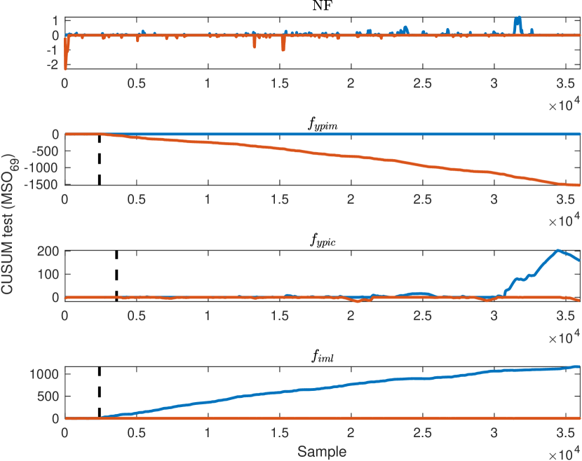
Figure 22: Fault detection using CUSUM tests based on residual generator MSO₆₉.

IX Discussion

The engine case study show that structural methods is a useful approach to design grey-box RNN for residual generation. It is also shown how model-based approaches, such as CUSUM tests, can improve classification performance. Residual generators are anomaly classifiers modeling nominal system operation represented in training data. Since an anomaly classifier only detects when observed data deviates from nominal training data, there are some important aspects to take into consideration when drawing conclusions from triggered residuals, i.e. residual outputs that deviate from the nominal case.

IX-A Training Data

The accuracy of a data-driven classifier depends on the quality of training data. If training data are not representative of nominal operation the neural network-based residual generators are not only likely to trigger an alarm when there is a fault in the system but also when the current system operation is not represented in training data. This means that a triggered residual can be explained by a fault or that the system is operating in a different mode with respect to training data.

IX-B Fault sensitivity

Another known problem is sufficient excitation of all signals in training data. Evaluation of fault detection performance show that the trained grey-box RNN are overall best at detecting faults strongly affecting the predicted sensor output, even though they are sensitive to the other faults as well. Some measured states such as temperatures are slowly varying over time which requires more extensive data collection to cover the expected variations during nominal operation Making sure that training data is representative of all relevant system operation is necessary to reduce the risk of false alarms but also assure that residuals become sensitive to faults affecting those signals. One solution is to design different residuals with varying sampling rates to capture fast and slow dynamics and, thus, be able to detect different types of faults.

IX-C Improve Fault Isolation Performance Using Data-Driven Fault Class Modeling

Even though the residual generators are trained using only nominal training data, it is possible that data from different fault scenarios are available or will be collected over time. Thus, it is relevant to take this data into consideration to improve fault classification performance when new faults are detected.

It is possible to distinguish between the two faults because they are affecting the residuals in different ways. Feeding the residual outputs into an multi-class classifier to compute fault hypotheses that can explain the observed data. Open set classification approaches proposed in, e.g., [3] and [16], could be used to handle unknown fault classes and incremental learning of fault models to improve classification performance over time.

X Conclusions

Unknown fault classes and limited training data complicate data-driven fault diagnosis. In addition, developing sufficiently accurate models for designing model-based residuals is a difficult and time consuming process. Using grey-box RNN for residual generation is shown to be a promising approach to take advantage of both model-based fault diagnosis methods and data-driven model training. The use of grey-box RNN makes it possible to incorporate available physical insights about the system into data-driven models where tools from model-based diagnosis like structural analysis can help automate the residual generator design process. The results from the engine case study show that the generated grey-box RNN are able to capture the dynamic behavior of the engine and can be used to detect and classify different types of faults.

Future work will further investigate how the model structure of the different grey-box neural networks affect their fault detection performance. It is also important to investigate how to optimize fault sensitivity when training the grey-box RNN to maximize fault detection but also make sure that faults are decoupled according to the structural model.

References

- [1] L. Ljung, System Identification (2nd Ed.): Theory for the User. USA: Prentice Hall PTR, 1999.
- [2] S. Qin, “Survey on data-driven industrial process monitoring and diagnosis,” Annual reviews in control, vol. 36, no. 2, pp. 220–234, 2012.
- [3] D. Jung, K. Ng, E. Frisk, and M. Krysander, “Combining model-based diagnosis and data-driven anomaly classifiers for fault isolation,” Control Engineering Practice, vol. 80, pp. 146–156, 2018.
- [4] L. Dong, L. Shulin, and H. Zhang, “A method of anomaly detection and fault diagnosis with online adaptive learning under small training samples,” Pattern Recognition, vol. 64, pp. 374–385, 2017.
- [5] C. Sankavaram, A. Kodali, K. Pattipati, and S. Singh, “Incremental classifiers for data-driven fault diagnosis applied to automotive systems,” IEEE Access, vol. 3, pp. 407–419, 2015.
- [6] G. Acuña, F. Cubillos, J. Thibault, and E. Latrille, “Comparison of methods for training grey-box neural network models,” Computers & Chemical Engineering, vol. 23, pp. S561–S564, 1999.
- [7] E. Pintelas, I. Livieris, and P. Pintelas, “A grey-box ensemble model exploiting black-box accuracy and white-box intrinsic interpretability,” Algorithms, vol. 13, no. 1, p. 17, 2020.
- [8] D. Jung, “Isolation and localization of unknown faults using neural network-based residuals,” in Proceedings of the Annual Conference of the PHM Society, vol. 11, no. 1, 2019.
- [9] I. Arsie, C. Pianese, and M. Sorrentino, “A procedure to enhance identification of recurrent neural networks for simulating air–fuel ratio dynamics in si engines,” Engineering Applications of Artificial Intelligence, vol. 19, no. 1, pp. 65–77, 2006.
- [10] C. Aggarwal, “Neural networks and deep learning,” Springer, vol. 10, pp. 978–3, 2018.
- [11] B. Pulido, J. Zamarreño, A. Merino, and A. Bregon, “State space neural networks and model-decomposition methods for fault diagnosis of complex industrial systems,” Engineering Applications of Artificial Intelligence, vol. 79, pp. 67–86, 2019.
- [12] J. Cassar and M. Staroswiecki, “A structural approach for the design of failure detection and identification systems.” in IFAC Conference on Control of Industrial Systems (Control for the Future of the Youth), Belfort, France, 20-22 May, vol. 30, no. 6, 1997, pp. 841 – 846.
- [13] B. Pulido and C. González, “Possible conflicts: a compilation technique for consistency-based diagnosis,” IEEE Transactions on Systems, Man, and Cybernetics, Part B (Cybernetics), vol. 34, no. 5, pp. 2192–2206, 2004.
- [14] M. Krysander, J. Åslund, and M. Nyberg, “An efficient algorithm for finding minimal overconstrained subsystems for model-based diagnosis,” IEEE Transactions on Systems, Man, and Cybernetics-Part A: Systems and Humans, vol. 38, no. 1, pp. 197–206, 2007.
- [15] E. Frisk, M. Krysander, and D. Jung, “A toolbox for analysis and design of model based diagnosis systems for large scale models,” IFAC-PapersOnLine, vol. 50, no. 1, pp. 3287–3293, 2017.
- [16] W. Scheirer, de Rezende R., A. Sapkota, and T. Boult, “Toward open set recognition,” IEEE transactions on pattern analysis and machine intelligence, vol. 35, no. 7, pp. 1757–1772, 2012.
- [17] M. Atoui, A. Cohen, S. Verron, and A. Kobi, “A single bayesian network classifier for monitoring with unknown classes,” Engineering Applications of Artificial Intelligence, vol. 85, pp. 681–690, 2019.
- [18] A. Bernieri, M. D’apuzzo, L. Sansone, and M. Savastano, “A neural network approach for identification and fault diagnosis on dynamic systems,” IEEE transactions on Instrumentation and Measurement, vol. 43, no. 6, pp. 867–873, 1994.
- [19] W. Zhang, G. Biswas, Q. Zhao, H. Zhao, and W. Feng, “Knowledge distilling based model compression and feature learning in fault diagnosis,” Applied Soft Computing, vol. 88, p. 105958, 2020.
- [20] M. Bidarvatan, V. Thakkar, M. Shahbakhti, B. Bahri, and A. Aziz, “Grey-box modeling of hcci engines,” Applied Thermal Engineering, vol. 70, no. 1, pp. 397–409, 2014.
- [21] M. Witczak, “Advances in model-based fault diagnosis with evolutionary algorithms and neural networks,” International Journal of Applied Mathematics and Computer Science, vol. 16, no. 1, p. 85, 2006.
- [22] L. Lu, Y. Tan, D. Oetomo, I. Mareels, E. Zhao, and S. An, “On model-guided neural networks for system identification,” in 2019 IEEE Symposium Series on Computational Intelligence (SSCI), 2019, pp. 610–616.
- [23] R. Rahimilarki and Z. Gao, “Grey-box model identification and fault detection of wind turbines using artificial neural networks,” in 2018 IEEE 16th International Conference on Industrial Informatics (INDIN). IEEE, 2018, pp. 647–652.
- [24] K. Tidriri, N. Chatti, S. Verron, and T. Tiplica, “Bridging data-driven and model-based approaches for process fault diagnosis and health monitoring: A review of researches and future challenges,” Annual Reviews in Control, vol. 42, pp. 63–81, 2016.
- [25] Y. Lu, A. Zhong, Q. Li, and B. Dong, “Beyond finite layer neural networks: Bridging deep architectures and numerical differential equations,” in International Conference on Machine Learning, 2018, pp. 3276–3285.
- [26] T. Chen, Y. Rubanova, J. Bettencourt, and D. Duvenaud, “Neural ordinary differential equations,” in Advances in neural information processing systems, 2018, pp. 6571–6583.
- [27] Z. Wu, J. Li, M. Cai, Y. Lin, and W. Zhang, “On membership of black-box or white-box of artificial neural network models,” in 2016 IEEE 11th Conference on Industrial Electronics and Applications (ICIEA), 2016, pp. 1400–1404.
- [28] R. Hofmann, V. Halmschlager, M. Koller, G. Scharinger-Urschitz, F. Birkelbach, and H. Walter, “Comparison of a physical and a data-driven model of a packed bed regenerator for industrial applications,” Journal of Energy Storage, vol. 23, pp. 558–578, 2019.
- [29] A. Choudhary, J. Lindner, E. Holliday, S. Miller, S. Sinha, and W. Ditto, “Physics-enhanced neural networks learn order and chaos,” Physical Review E, vol. 101, no. 6, p. 062207, 2020.
- [30] J. Zamarreno, P. Vega, L. Garcıa, and M. Francisco, “State-space neural network for modelling, prediction and control,” Control Engineering Practice, vol. 8, no. 9, pp. 1063–1075, 2000.
- [31] J. De Kleer and B. Williams, “Diagnosing multiple faults,” Artificial intelligence, vol. 32, no. 1, pp. 97–130, 1987.
- [32] E. Page, “Continuous inspection schemes,” Biometrika, vol. 41, no. 1/2, pp. 100–115, 1954.
- [33] A. Dulmage and N. Mendelsohn, “Coverings of bipartite graphs,” Canadian Journal of Mathematics, vol. 10, pp. 517–534, 1958.
- [34] E. Frisk, A. Bregon, J. Aslund, M. Krysander, B. Pulido, and G. Biswas, “Diagnosability analysis considering causal interpretations for differential constraints,” IEEE Transactions on Systems, Man, and Cybernetics-Part A: Systems and Humans, vol. 42, no. 5, pp. 1216–1229, 2012.
- [35] U. Ascher and L. Petzold, Computer methods for ordinary differential equations and differential-algebraic equations. Siam, 1998, vol. 61.
- [36] L. Eriksson, S. Frei, C. Onder, and L. Guzzella, “Control and optimization of turbo charged spark ignited engines,” in IFAC World Congress, 2002.
- [37] K. Ng, E. Frisk, and M. Krysander, “Design and selection of additional residuals to enhance fault isolation of a turbocharged spark ignited engine system,” in 7th International Conference on Control, Decision and Information Technologies (CoDIT’20). IEEE, 2020.
- [38] L. Eriksson, “Modeling and control of turbocharged si and di engines,” OGST-Revue de l’IFP, vol. 62, no. 4, pp. 523–538, 2007.
- [39] A. Paszke, S. Gross, S. Chintala, G. Chanan, E. Yang, Z. DeVito, Z. Lin, A. Desmaison, L. Antiga, and A. Lerer, “Automatic differentiation in pytorch,” in NIPS-W, 2017.
- [40] J. Diederik and P. Kingma, “Adam: A method for stochastic optimization,” in 3rd international conference for learning representations, San Diego, 2015.
- [41] L. van der Maaten and G. Hinton, “Visualizing data using t-sne,” Journal of machine learning research, vol. 9, no. Nov, pp. 2579–2605, 2008.
- [42] B. Lakshminarayanan, A. Pritzel, and C. Blundell, “Simple and scalable predictive uncertainty estimation using deep ensembles,” in Advances in neural information processing systems, 2017, pp. 6402–6413.