Measuring the polarization of boosted, hadronic $W$ bosons with jet substructure observables

Abstract

In this work, we present a new technique to measure the longitudinal and transverse polarization fractions of hadronic decays of boosted $W$ bosons. We introduce a new jet substructure observable denoted as $p_{\theta}$, which is a proxy for the parton level decay polar angle of the $W$ boson in its rest-frame. We show that the distribution of this observable is sensitive to the polarization of $W$ bosons and can therefore be used to reconstruct the $W$ polarization in a model-independent way. As a test case, we study the efficacy of our technique on vector boson scattering processes at the high luminosity Large Hadron Collider and we find that our technique can determine the longitudinal polarization fraction to within $\pm 0.15$. We also show that our technique can be used to identify the parity of beyond Standard Model scalar or pseudo-scalar resonances decaying to $W$ bosons with just 20 events.

1 Introduction and motivation

In the Standard Model (SM), the $W$ and $Z$ bosons acquire mass through the Higgs mechanism. An important prediction of the SM is that the residual Higgs boson couples to $W$ bosons in proportion to the mass of the $W$. At high energies, longitudinal gauge-boson scattering would violate unitarity in the absence of the SM Higgs boson or if the Higgs boson couplings were not precisely the same as those predicted in the SM. The discovery of the $125$ GeV scalar boson at the Large Hadron Collider (LHC) Aad:2012tfa ; Chatrchyan:2012ufa is an indication that we might have discovered the long sought after Higgs boson. However, much still remains to be done to confirm that this is indeed the Higgs boson of the SM. In particular, the couplings of this Higgs-like object to the $W$ and $Z$ bosons needs to be measured precisely, in order to confirm the 125 GeV scalar has fully resolved the would-be unitarity violation in the absence of a SM Higgs. Moreover, naturalness considerations Morrissey:2009tf ; Farina:2013mla ; Feng:2013pwa ; deGouvea:2014xba motivate theories such as supersymmetry Martin:1997ns or composite Higgs models Csaki:2018muy which in turn suggest that other new states such as heavy Higgs bosons or massive techni-hadrons should play a role in electroweak symmetry breaking (EWSB) and perhaps play a role in restoration of unitarity in high energy longitudinal gauge-boson scattering.

In these models, one typically encounters scenarios where the heavy resonance (either a heavy Higgs or a heavy techni-rho type object) decays to a pair of predominantly longitudinally polarized $W$ or $Z$ bosons Kilian:2014zja ; Kilian:2015opv . Discovery of a resonance of $WW$, $WZ$ or $ZZ$ pairs would be an exciting signature of such new physics. However, in order to fully understand the role of the new physics on EWSB, it will be important to measure the polarization of the $W$ and $Z$ bosons.

In this work, we propose a technique which will enable collider experiments to measure the polarization fractions of hadronically decaying $W$ bosons. There are two distinct advantages to doing so which we list below.

• At present, polarization fractions can be inferred in a model independent way only when at least one of the gauge bosons decays leptonically (about $20\%$ of the time). For example, CMS has measured $W$ boson polarization in leptonic $W+$jet events Chatrchyan:2011ig and ATLAS has measured the polarization of $W$s in semi-leptonic $t\overline{t}$ events Aad:2012ky . However, it would greatly increase our statistical grasp of the polarization fractions, if we were able to measure the polarization of hadronic $W$ bosons.

• In order to test unitarity in vector boson scattering (VBS), we would ideally like to measure the polarization fraction of both the outgoing weak bosons in a scattering process, which would allow us to infer correlations in the spins Han:2009em . In principle, one could simultaneously measure the polarization of both weak bosons in fully-leptonic $WZ$ or $ZZ$ scattering Ballestrero:2019qoy , but these processes have significantly lower cross-sections than $WW$ scattering Brehmer:2014dnr . However, in fully leptonic $WW$ scattering processes, kinematic ambiguities due to missing neutrinos make the polarization measurement very difficult. Measuring the polarization of hadronic $W$ decays would enable a simultaneous polarization measurement of both $W$ bosons in VBS, in either the semi-leptonic or fully hadronic decay channels.

In this work, we will make use of the technique of $N$-subjettiness Thaler:2010tr , which has been used to effectively tag hadronically decaying boosted $W$ bosons. We adapt the technique to additionally measure $W$ polarization. We show that we can use the subjets identified using $N$-subjettiness to construct a new variable whose distribution is sensitive to the polarization fraction of the $W$ bosons.

This paper is organized as follows: in Sec. 2, we review decay kinematics of a hadronically decaying $W$ boson in the rest-frame and the lab-frame at parton level and then at the hadron level. We show how a particular lab-frame observable at parton level (namely the ratio of the energy difference between the quarks from $W$ decay to the $W$ boson momentum), is a measure of the rest-frame decay polar angle and is hence sensitive to the polarization of the $W$ boson. We also discuss how showering, hadronization and jet clustering effects impact the distribution of this observable. In Sec. 3, we construct an observable proxy variable, which we denote as $p_{\theta}$, for the decay polar angle using jet substructure techniques. In Sec. 4, we discuss the distortions of this proxy variable and we build templates of the distribution of this proxy variable for longitudinally-polarized and transversely-polarized $W$ bosons. In Sec. 5, we discuss how to use the proxy variable to measure polarization of $W$ bosons, and two applications of this technique (i) to reconstruct the polarization fraction of mixed-polarization samples of hadronically-decaying $W$ bosons taking the test case of VBS and (ii) for discriminating between scalar/pseudo-scalar resonances decaying to $W$ bosons which are purely longitudinal/transverse. In Sec. 6, we discuss some backgrounds that can affect the extraction of the polarization fraction of the sample and how to overcome these. Finally, we summarize and conclude in Sec. 7. In appendix A, we discuss details of the models used to generate our calibration samples of longitudinal and transverse $W$ bosons.

2 Measuring $W$-polarization via hadronic decays

In order to understand the effect of $W$-polarization on its hadronic decay products, we will first review the well-known kinematic distribution of the decay products of $W$-bosons of a given helicity at parton level. The $W$ rest-frame distributions can be easily understood from angular momentum conservation principles. We will see that there is a clear distinction in the angular distribution of the decay products depending on whether the $W$ boson is longitudinally or transversely polarized. However, since we will eventually be interested in studying jets initiated by quarks, we would like to study lab-frame observables that can give us direct inferences of the $W$ rest-frame distributions, in a manner which does not require us to reconstruct the $W$ rest-frame to infer the rest-frame observables. This is because, in general, errors in the lab-frame observables propagate into the reconstruction of typical rest-frame observables in a non-trivial way, significantly complicating the prediction of uncertainties on rest-frame observables.

2.1 Parton level angular distributions

Consider the decay $W^{+}\rightarrow u\overline{d}$ in the rest-frame of the $W^{+}$, as shown in Fig. 1. The angular distribution of the decay products depends upon one degree of freedom in the decay plane, which we can choose to be the decay polar angle $\theta_{*}$, defined as the angle between the up-quark momentum axis and the axis along which the $W^{+}$ is boosted in the lab-frame. For a given lab-frame helicity ($h$), the amplitude for $W^{+}$ decay has the following dependence on $\theta_{*}$,

$$\mathcal{M}_{\pm}\propto\frac{1\mp\cos\theta_{*}}{2},$$ (1)

$$\mathcal{M}_{0}\propto-\frac{\sin\theta_{*}}{\sqrt{2}}.$$ (2)

Here, the subscripts $(\pm,0)$ refer to the helicity of the $W^{+}$. Identical expressions hold for the helicity amplitudes of $W^{-}$ decays, with the decay polar angle defined to be the angle between the down quark momentum axis in the $W^{-}$ rest-frame and the $W^{-}$ boost axis.

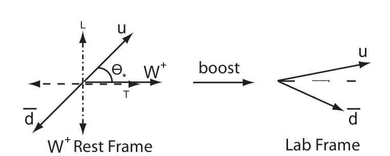
Figure 1: Left: The polar angle $\theta_{*}$ of the decay products of the $W^{+}$ as defined in the rest-frame of the $W^{+}$. For reference, the $W$ momentum axis in the lab-frame is shown. The dashed (dot-dashed) line shows the preferred orientation of the decay products of the $W^{+}$ for transverse (longitudinal) polarizations. Right: Upon boosting to the lab-frame, the up and anti-down quarks can display an asymmetry in energy. For transverse $W$ bosons, this asymmetry is maximal, whereas for longitudinal $W$ bosons, the energy sharing is preferentially equal, leading to a minimal asymmetry. The lab-frame energy difference between the quarks is related to the angle $\theta_{*}$ by Eq. 3.

We note an interesting feature of these angular distributions that distinguishes the longitudinal and transverse modes of the $W^{+}$ decay. For the longitudinal modes, the decay products tend to preferentially align themselves perpendicular to the boost axis of the $W^{+}$, whereas for the transverse modes the decay products tend to align in parallel (as measured by the quark momentum) or anti-parallel to the boost axis of the $W^{+}$. This feature will be the key to distinguishing $W$ polarizations in the lab-frame.

Boosting the $W^{+}$ decay products to the lab-frame yields the configuration shown in Fig. 1; because of the preferentially-(anti-)parallel decays, the transverse $W^{+}$ decay products will tend to have a larger energy difference between the quark and anti-quark (as well as a larger opening angle in the lab-frame). We will try to exploit the energy difference as a lab-frame observable that could probe the polarization of the $W^{+}$.

2.2 Energy Difference

We find a simple relationship between $\theta_{*}$ and $\Delta E\equiv E_{q}-E_{\overline{q}}$, the energy difference between the quark and the anti-quark in the lab-frame at parton level,

$$\cos\theta_{*}=\frac{\Delta E}{p_{W}}.$$ (3)

Here, $p_{W}$ is the momentum of the $W^{+}$ in the lab-frame. This equation relates the rest-frame observable $\cos\theta_{*}$, in a simple way, to lab-frame observables. Using the expected distributions of $\cos\theta_{*}$, we can see that longitudinally polarized $W^{+}$ bosons will tend to prefer an equal distribution of energies between the quark and the anti-quark, whereas transverse $W$ bosons would prefer to create a large asymmetry between the two. This relationship is well preserved under showering and hadronization, though no longer exact, as we will discuss in detail in Sec. 2.3.

In general, all the helicity states of the $W^{+}$ will interfere with each other Buckley:2007th ; Buckley:2008pp ; Ballestrero:2017bxn . However, when we integrate over the full decay azimuthal angles for $W$-decay, the interference terms drop out. We are thus left with a simple expression for the distribution of the $W^{+}$ decay rate as a function of its decay polar angle,

$$\frac{1}{\sigma}\frac{d\sigma}{d\cos\theta_{*}} =f_{+}\frac{3}{8}\left(1-\cos\theta_{*}\right)^{2}+f_{-}\frac{3}{8}\left(1+\cos\theta_{*}\right)^{2}+f_{0}\frac{3}{4}\left(\sin\theta_{*}\right)^{2}$$ (4)

$$=f_{T}\frac{3}{8}\left(1+\cos^{2}\theta_{*}\right)+f_{L}\frac{3}{4}\left(1-\cos^{2}\theta_{*}\right)-f_{D}\frac{3}{4}\cos\theta_{*}.$$ (5)

Here, in the first line $f_{h}$ corresponds to the polarization fractions of the helicity state $h=(1,0,-1)$, and the normalizations are chosen so that $f_{+}+f_{-}+f_{0}=1$. In the second line, we have defined the transverse polarization sum $f_{T}=f_{+}+f_{-}$ and the transverse polarization difference $f_{D}=f_{+}-f_{-}$, and we have shifted notation to write the longitudinal polarization fraction as $f_{L}\equiv f_{0}$.

In general, application of cuts will prevent us from observing cross-sections integrated over the entire range of azimuthal angles and this will restore some of the interference terms between the various polarization states of the $W^{+}$ Mirkes:1994eb ; Stirling:2012zt ; Belyaev:2013nla . When the $W^{+}$ decays to jets, if we do not make any attempt to identify observables like the jet charge, we lose information about the quark-anti-quark difference. Thus, we are restricted to measuring only the absolute value of the energy difference $|\Delta E|$. Moreover, since we would no longer be able to distinguish between $W^{+}$ and $W^{-}$, we would be measuring polarization fractions for a combined sample of $W^{+}$ and $W^{-}$.

Upon restricting ourselves to a measurement of $|\cos\theta_{*}|$, the expected distribution is given by

$$\frac{1}{\sigma}\frac{d\sigma}{d|\cos\theta_{*}|}=f_{T}\frac{3}{4}\left(1+|\cos\theta_{*}|^{2}\right)+f_{L}\frac{3}{2}\left(1-|\cos\theta_{*}|^{2}\right).$$ (6)

This expression holds for both $W^{+}$ and $W^{-}$, thus we can use the measured energy difference distribution to extract the transverse polarization fraction $f_{T}$ and the longitudinal polarization fraction $f_{L}$ of all $W$ bosons in a sample. Since, $f_{T}+f_{L}=1$, the entire distribution is parameterized by a single parameter, which we can choose to be $f_{L}$, i.e. the longitudinal polarization fraction.

In $WW$ scattering events, we could use this technique of polarization measurements to measure correlations between the $W$ boson helicities by constructing the joint distribution $\frac{1}{\sigma}\frac{d^{2}\sigma}{d|\cos\theta^{1}_{*}|d|\cos\theta^{2}_{*}|}$ where $\theta^{1}_{*}$ and $\theta^{2}_{*}$ are the decay polar angles of the two $W$ bosons in the event, as defined in their respective rest-frames.

2.3 Showering, hadronization and clustering effects

The quarks from $W$ decay undergo showering and hadronization and are detected as jets. In principle, to the extent that the individual quark jets can be resolved and their energy difference identified, we can construct the distribution $\frac{1}{\sigma}\frac{d\sigma}{d|\cos\theta_{*}|}$ and at lowest order in QCD we would expect it to have the behavior given by Eq. 6. By fitting our observations to this distribution we can extract the polarization fractions of the $W$ bosons.

For high energy $W$ bosons, the jets from $W$-decay are highly collimated and most often identified as a single fat-jet. To construct the angular distribution, we would need to:

• Identify the fat-jets which correspond to $W$ bosons using boosted-object tagging techniques. We denote the magnitude of momentum of this fat-jet as $p_{W}^{\textrm{\tiny{reco}}}$ which is a hadron level reconstruction of the $W$ momentum.

• For the jets that correspond to $W$ bosons, we need to identify the subjet energy difference that would correspond to the parton level energy difference. We denote the absolute value of this energy difference as $|\Delta E^{\textrm{\tiny{reco}}}|$.

• Once we have $|\Delta E^{\textrm{\tiny{reco}}}|$ and $p_{W}^{\textrm{\tiny{reco}}}$, we take the ratio and use this to define a proxy variable $p_{\theta}$ for the partonic level $W$ decay angle $|\cos\theta_{*}|$ as,

  $$p_{\theta}=\frac{|\Delta E^{\textrm{\tiny{reco}}}|}{p_{W}^{\textrm{\tiny{reco}}}}.$$ (7)

In principle, any substructure observable that can be used to mimic the energy difference of the parton level objects could be used to construct a proxy for $|\cos\theta_{*}|$. In the next section, we will discuss how to construct $p_{\theta}$ using the $N$-subjettiness technique. Once we have event-by-event measurements of such a proxy variable, we can then construct a distribution for a given event sample that should correspond to Eq. 6. In principle, it then becomes possible to fit the expected distribution to the form in Eq. 6 and extract the polarization fractions of transverse ($f_{T}$) and longitudinal gauge bosons ($f_{L}$) as fit coefficients.

In practice several effects will alter the distribution of the proxy variable $p_{\theta}$ relative to the naive parton level distribution of $|\cos\theta_{*}|$ discussed above:

• The decay products of the $W$ are color connected and so higher order QCD corrections will distort the angular distribution of the final state subjet axes relative to the tree-level partonic prediction.

• Initial state radiation (ISR) and pile-up effects distort our mapping of the subjets to the expected parton level kinematics.

• Detector effects such as jet energy scale uncertainty and inability to detect neutrinos prevent ideal reconstruction of the subjet momenta.

• Any cuts that (directly or indirectly) depend on the azimuthal angle of $W$ decay can distort the distributions expected in Eq. 6 by restoring the interference terms between the various helicity states.

• Pruning of jets, which is necessary for both pile-up removal as well as accurate jet mass reconstruction, will lead to removal of soft and wide-angle subjets. This becomes especially pertinent for events which have a large value of $|\cos\theta_{*}|$ at parton level, since, upon boosting to the lab-frame, one of the quarks will be soft and emitted at a wide angle in the lab-frame. The subjet resulting from this quark will often be removed during pruning. When attempting to tag such a jet as arising from a $W$ boson, one would see only a single prong, thus leading to a misclassification of the jet.

In the next section, we describe the construction of $p_{\theta}$ using $N$-subjettiness techniques. We will determine the efficacy of $p_{\theta}$ as a proxy variable for $|\cos\theta_{*}|$, and we will see how the effects mentioned above distort the $p_{\theta}$ distribution relative to the $|\cos\theta_{*}|$ distribution for a given event sample.

Once we reliably understand the physics of the distortions, we can use the distributions of $p_{\theta}$ for longitudinal and transverse $W$ bosons as templates to fit the distribution for a mixed polarization sample to a linear combination of the templates to extract the $W$ boson polarization fractions.

3 $N$-subjettiness and the proxy variable $p_{\theta}$

We begin by identifying a fat-jet in an event by using a clustering algorithm such as Cambridge-Aachen Dokshitzer:1997in ; Wobisch:1998wt with a large radius $R_{0}=1.0$. The original $N$-subjettiness technique Thaler:2010tr can be used to identify the number of hard centres of energy within a fat-jet.

One starts by defining a collection of variables $\tau_{N}$, where $N$ = 1, 2, 3 … denotes the number of candidate subjets. For each $N$ we construct the corresponding variables as

$$\tau_{N}=\min\limits_{\hat{n}_{1},\hat{n}_{2},...,\hat{n}_{N}}\tilde{\tau}_{N},\textrm{ where},\tilde{\tau}_{N}=\frac{1}{d_{0}}\sum_{k}p_{T,k}\textrm{ min}\{(\Delta R_{1,k}),(\Delta R_{2,k}),...,(\Delta R_{N,k})\}.$$ (8)

Here, the index $k$ runs over the constituent particles in a given fat-jet, $p_{T,k}$ are their transverse momenta, $\Delta R_{J,k}=\sqrt{(\Delta\eta)^{2}+(\Delta\phi)^{2}}$ is the distance in the rapidity-azimuth plane between a candidate subjet $J$ and the constituent particle $k$.

The minimization in the definition of $\tau_{N}$ is performed over $N$ candidate subjet axes denoted as $\hat{n}_{i}$ (where $i$ goes from 1 … $N$). The normalization factor $d_{0}$ is given as,

$$d_{0}=\sum_{k}p_{T,k}R_{0},$$

where $R_{0}$ is the jet-radius used in the original jet-clustering algorithm. It is easy to see from this definition that fat-jets with $\tau_{N}\approx 0$ have a maximum of $N$ subjets and fat-jets having $\tau_{N}\gg 0$ have at least $N$+1 subjets.

The variables $\tau_{N}$ can be used to construct a discriminator that can help identify on a statistical basis whether a fat-jet is produced from a boosted object (such as a decaying $W$ bosons) or from QCD. In the case of $W$ bosons, one would attempt to construct the ratio $\tau_{2}/\tau_{1}$. Small values of this ratio indicate a fat-jet that is more $W$-like, whereas larger values of this ratio indicate a more QCD-like jet.

Prior to the construction of $\tau_{N}$, it is important to determine the candidate subjet axes using the exclusive $k_{T}$ algorithm Catani:1993hr ; Ellis:1993tq , which partitions the jet constituent space into $N$ Voronoi regions, containing the subjet axes. This algorithm provides one Voronoi region containing one candidate subjet axis when $\tau_{1}$ is calculated, and will give two Voronoi region containing (respectively) either of the two subjet axes when $\tau_{2}$ is calculated and so on. These candidate subjet axes will act as initial seeds for Lloyd’s algorithm Lloyd82leastsquares to generate, upon recursion, a new set of subjet axes that will minimise $\tau_{N}$. This new set of subjet axes will lie in the centre of the new Voronoi regions. Adding up the energy of the constituent particles in the Voronoi regions gives us the corresponding subjet energy. For candidate $W$ fat-jets, we can use the subjet axis that minimize $\tau_{2}$ to identify the Voronoi regions, the candidate subjets, and their corresponding energies.

Thus, we can construct $|\Delta E^{\textrm{\tiny{reco}}}|$ using the $N$-subjettiness method, and we can find $p_{W}^{\textrm{\tiny{reco}}}$ from the momentum of the fat-jet obtained from our clustering algorithm. Finally, we can define our proxy variable $p_{\theta}$ using Eq. 7.

4 Calibration of the proxy variable

4.1 Construction of longitudinal and transverse $W$ boson calibration sample events

In order to calibrate our procedure of separation of differently polarized $W$ bosons using the proxy variable $p_{\theta}$, we need to setup two “calibration samples” - one containing fully longitudinally polarized $W$ bosons, which we denote as $\mathcal{S}_{L}$, and the other containing fully transversely polarized $W$ bosons, which we denote as $\mathcal{S}_{T}$.

Using MadGraph 5 Alwall:2014hca , we generate the process: $pp\rightarrow\phi\rightarrow W^{+}W^{-}\rightarrow jjjj$ at a center-of-mass energy $\sqrt{s}$ $=$ 13 TeV. Here, $\phi$ is a new fictitious particle which we introduce for the purpose of generating the calibration samples. Using a scalar field, $\phi$, we can generate purely longitudinally polarized $W$ bosons, and using a pseudo-scalar field, we can generate purely transversely polarized $W$ bosons. This result is not automatically obvious, details of the models and the consequent $W$-polarization fractions are discussed in appendix A.

We then implement the following procedure:

1. We generate 1 million events each, with an intermediate scalar $\phi$ and a pseudo-scalar $\phi$, using MadGraph. At the generator level, we demand that the $W$ bosons have transverse momentum $p_{T}$ between 800 GeV and 1000 GeV.

2. We shower and hadronize these events in Pythia 8 Sjostrand:2006za ; Sjostrand:2007gs .

3. We then cluster the final-state particles using the Cambridge-Aachen algorithm in FastJet Cacciari:2011ma with a jet radius $R_{0}=1.0$ and also implement pruning Ellis:2009su to remove soft tracks which would be inseparable from pileup contributions. We use the pruning parameters $z_{\textrm{cut}}=0.1$ and $\Delta R_{\textrm{cut}}=0.25$.

By matching the momentum of the leading $p_{T}$ fat-jets after clustering with the parton level truth information, we can identify the jets corresponding to the $W$ bosons. We then impose the following tagging cuts on the $W$ jets:

• Mass cut: 60 GeV $<M_{J}<$ 100 GeV, where $M_{J}$ is the mass of the pruned fat-jet,

• Mass-drop cut Butterworth:2008iy : $\mu^{\textrm{cut}}$ $<$ 0.25 and $y^{\textrm{cut}}$ $<$ 0.09,

• $N$-subjettiness cut: $\tau_{2}/\tau_{1}<0.3$.

We denote the surviving events in our samples after imposition of these cuts as $\mathcal{S}_{L}^{\prime}$ and $\mathcal{S}_{T}^{\prime}$.

Note that, for the purpose of our analysis:

• We have not added min bias to simulate the effects of pile-up. However, we expect that the pruning algorithm we are employing would be able to subtract most of the pile-up contribution to the jet observables CMS:2014ata .

• We have not performed a detector simulation which would result in smearing of the final-state particles momenta. The dominant effect associated with realistic detector effects is the jet energy scale uncertainty ATLAS:2013wma ; Khachatryan:2016kdb . However, since the $p_{\theta}$ observable we are looking at is a ratio of energy scales, we expect that our results will only be mildly affected by detector smearing.

• We have taken care to remove neutrinos when clustering the final-state particles.

Working with the $\mathcal{S}^{\prime}$ samples, we can use the $N$-subjettiness routine in FastJet to recover the two subjet four-vectors and corresponding energies within the tagged $W^{+}$ jet. We then use these to construct out proxy variable $p_{\theta}$, as defined in Eq. 7.

This procedure yields event-by-event parton level truth information about $|\cos\theta_{*}|$ and the corresponding reconstructed proxy variable $p_{\theta}$ at hadron level. We can now verify the efficacy of our proxy variable and find the difference between the distribution of the proxy variable for the samples $\mathcal{S}_{L}^{\prime}$ and $\mathcal{S}_{T}^{\prime}$.

4.2 Effect of pruning and tagging on the $|\cos\theta_{*}|$ distribution and the tagging efficiency

Before we discuss the efficacy of our proxy variable, we would like to understand the distortions in the $|\cos\theta_{*}|$ distribution that arise because of the cuts that we have imposed in going from the samples $\mathcal{S}$ to $\mathcal{S}^{\prime}$.

As we go from the original samples $\mathcal{S}_{L}$ and $\mathcal{S}_{T}$ to the samples $\mathcal{S}_{L}^{\prime}$ and $\mathcal{S}_{T}^{\prime}$, we lose a significant number of events. The sample $\mathcal{S}_{L}^{\prime}$ has 602155 events and the $\mathcal{S}_{T}^{\prime}$ sample has 475386 events. We thus interpret the overall tagging efficiency of longitudinal $W$ bosons as $\epsilon_{L}=60.2\%$ and that of transverse $W$ bosons to be $\epsilon_{T}=47.5\%$. It is interesting to ask if the difference in tagging efficiencies can be understood in terms of the differences in the partonic $|\cos\theta_{*}|$ distributions of longitudinal and transverse $W$ bosons.

In Fig. 2, we plot the fraction of $W$ bosons that survive the pruning and tagging cuts as a function of the partonic $|\cos\theta_{*}|$. The efficiency curve is nearly the same for both the longitudinal and transverse $W$ boson samples, so we have averaged them together in the figure. From the figure, we can see that the tagging efficiencies are nearly constant between 50-60% up to a value of $|\cos\theta_{*}|\simeq 0.8$, and for larger values of $|\cos\theta_{*}|$ the efficiency drops to between 30-40%.

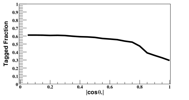
Figure 2: Tagging efficiencies of longitudinal and transverse $W$ bosons in the samples $S_{L}$ and $S_{T}$ as a function of their parton level decay polar angle $|\cos\theta_{*}|$. The efficiency drop for $|\cos\theta_{*}|\gtrsim 0.8$ can be attributed to the pruning algorithm removing a soft prong of the $W$ boson, which makes it fail the tagging cuts.

The drop in pruning and tagging efficiencies, in events with $|\cos\theta_{*}|\gtrsim 0.8$ at parton level, is easy to understand. For $|\cos\theta_{*}|\gtrsim 0.8$, at leading order, the partons are emitted in the $W$ rest-frame such that one is along the $W$ boost direction and the other is emitted opposite to the $W$ boost direction. Therefore, one would expect the parton opposite to the $W$ boost direction to result in a soft, wide-angle emission in the lab-frame. In general, such a wide-angle/soft prong would either be removed by pruning or would fall outside the candidate fat-jet intended to reconstruct the boosted $W$ boson. Thus, the resulting jets would appear to have a single prong, and such events are therefore naturally expected to fail the tagging cuts.

Quantitatively, for $|\cos\theta_{*}|\gtrsim 0.8$, we can estimate $z\equiv\textrm{min}(E_{1},E_{2})/p_{T}\simeq\frac{1}{2}(1-|\cos\theta_{*}|)<0.1$, where $E_{1}$ and $E_{2}$ are the energies of the two prongs of the $W$ and $p_{T}$ is the transverse momentum of the $W$ in the lab-frame. Thus, we can see that for such events $z<z_{\textrm{cut}}$. We can similarly show that the angle between the two prongs would be larger than $\Delta R_{\textrm{cut}}$. Thus, we would expect that events with $|\cos\theta_{*}|\gtrsim 0.8$ should fail the pruning and tagging cuts and therefore we expect that the $|\cos\theta_{*}|$ distribution for the pruned and tagged samples should deviate significantly from that of the untagged sample for values of $|\cos\theta_{*}|\gtrsim 0.8$.

However, given the expectation that for $|\cos\theta_{*}|\sim 1$, the $W$ bosons give rise to effectively single-prong jets, these jets should be indistinguishable from QCD jets. This raises a different question; why is the tagging efficiency so high for $|\cos\theta_{*}|\gtrsim 0.8$? The radiation pattern from the single prong jets appears to be such that about 30% of them pass the tagging cuts, but this efficiency is far higher than the QCD mistag rate, and therefore the radiation pattern must be characteristically different from typical QCD jets. We have not been able to diagnose this behavior in detail, but we present two possible hypotheses for the difference in the radiation pattern: first, it is possible that the color connection of the hard parton to the soft one increases the probability of relatively hard and wide-angle radiation relative to that in QCD production, where the connection is typically to a well-separated and fairly high-energy object. The second possibility is that this behaviour of the shower is an artifact of the Pythia8 procedure which is responsible for maintaining the invariant mass of the $W$ decay products. In either case, we can do no better than to adopt the efficiencies as measured in simulated data here. We will comment on possible procedures to check for this feature in experimental data in Sec. 4.5.

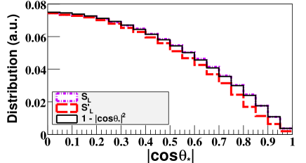
(a)

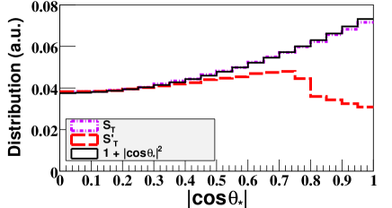
(b)

Figure 3: (a) Parton level truth information for the distributions of $|\cos\theta_{*}|$ for longitudinal $W$ bosons in the untagged longitudinal $W^{+}$ sample, $S_{L}$ and the tagged sample $S^{\prime}_{L}$. Also shown is the theoretically expected $(1-|\cos\theta_{*}|^{2})$ distribution which agrees very well with the $S_{L}$ distribution. (b) Same as the left panel, but with transverse $W$ bosons. Here, the theoretically expected distribution is $(1+|\cos\theta_{*}|^{2})$. In both cases, the pruned and tagged (primed) $|\cos\theta_{*}|$ distributions are normalized to agree in the first bin with the corresponding pre-tagging (unprimed) distribution in order to highlight the shape distortion due to pruning and tagging. The shape distortion due to tagging cuts is more significant in the case of transverse $W$s simply because $W$ bosons with higher $|\cos\theta_{*}|$ at parton level are more likely to fail the tagging cuts after jet pruning.

We can now examine the effect of the tagging efficiencies on the $|\cos\theta_{*}|$ distributions for the longitudinal and transverse $W$ bosons. In Fig. 3(a), we have plotted the distributions of $|\cos\theta_{*}|$ for the $\mathcal{S}_{L}$ sample and $\mathcal{S}_{L}^{\prime}$ samples. We have normalized the $|\cos\theta_{*}|$ distribution for the $\mathcal{S}_{L}$ sample to unity. However, we have normalized the $|\cos\theta_{*}|$ distribution for the $\mathcal{S}_{L}^{\prime}$ sample to agree with the first bin of the $\mathcal{S}_{L}$ sample distribution, in order to highlight the shape distortion of the distribution due to pruning and tagging. We see that for the $\mathcal{S}_{L}$ sample, which has no cuts, the distribution follows a $1-|\cos\theta_{*}|^{2}$ behavior, as expected for a longitudinally polarized $W$ boson sample (see Eq. 6). This distribution has relatively few events above $|\cos\theta_{*}|\gtrsim 0.8$, hence there is little distortion in the shape of the distribution when going to the pruned and tagged $\mathcal{S}_{L}^{\prime}$ sample.

We have also plotted the $|\cos\theta_{*}|$ distributions for the $\mathcal{S}_{T}$ sample in Fig. 3(b). We see that the distribution follows a $1+|\cos\theta_{*}|^{2}$ behavior for $\mathcal{S}_{T}$, as expected for a transversely polarized $W$ boson sample. Once again we have normalized the $|\cos\theta_{*}|$ distribution to unity for the $\mathcal{S}_{T}$ sample, but we have normalized the distribution for the $\mathcal{S}_{T}^{\prime}$ sample to agree with the first bin of the $\mathcal{S}_{T}$ distribution. For the transverse $W$ boson case, since there are a significant number of events with $|\cos\theta_{*}|\gtrsim 0.8$, we see a large distortion in the distribution of $|\cos\theta_{*}|$ in the $\mathcal{S}_{T}^{\prime}$ sample relative to the $\mathcal{S}_{T}$ sample.

As compared to the $\mathcal{S}_{L}$ sample, the $\mathcal{S}_{T}$ sample has more events with quarks emitted along the $W$ boost direction. Hence the distortion in the shape of the distribution after applying pruning and tagging cuts is much more severe on the transversely polarized $W$ boson sample. The difference in the overall tagging efficiencies can also be easily understood in light of the discussion above; transverse $W$ bosons have larger opening angles and a greater energy difference between the primary decay products as compared to longitudinal $W$ bosons and are hence removed more often by the combination of pruning and tagging.

In general, the tagging efficiencies $\epsilon_{L}$ and $\epsilon_{T}$ are expected to be universal (production process independent) for all longitudinal and transverse $W$ bosons, respectively. However, we also expect that there will be some mild dependence of these efficiencies on the $p_{T}$ of the $W$ bosons.

4.3 Efficacy of our proxy variable

$\begin{array}[]{ccc}\includegraphics[width=156.49014pt]{ScalarTemplate_cos_0_1.pdf}&\includegraphics[width=156.49014pt]{ScalarTemplate_cos_1_2.pdf}&\includegraphics[width=156.49014pt]{ScalarTemplate_cos_2_3.pdf}\end{array}$

$\begin{array}[]{ccc}\includegraphics[width=156.49014pt]{ScalarTemplate_cos_3_4.pdf}&\includegraphics[width=156.49014pt]{ScalarTemplate_cos_4_5.pdf}&\includegraphics[width=156.49014pt]{ScalarTemplate_cos_5_6.pdf}\end{array}$

$\begin{array}[]{ccc}\includegraphics[width=156.49014pt]{ScalarTemplate_cos_6_7.pdf}&\includegraphics[width=156.49014pt]{ScalarTemplate_cos_7_8.pdf}&\includegraphics[width=156.49014pt]{ScalarTemplate_cos_8_9.pdf}\end{array}$

$\begin{array}[]{c}\includegraphics[width=156.49014pt]{ScalarTemplate_cos_9_10.pdf}\end{array}$

Figure 4: Efficacy of $p_{\theta}$ as a proxy variable for $|\cos\,\theta_{*}|$. Each panel shows a comparison between the values of parton level information of $|\cos\,\theta_{*}|$ with the constructed proxy variable $p_{\theta}$ for events in the $\mathcal{S}_{L}^{\prime}$ sample. We can see that $p_{\theta}$ is a good proxy for $|\cos\,\theta_{*}|\lesssim 0.8$. An explanation for why $p_{\theta}$ is not a good proxy variable for the large $|\cos\,\theta_{*}|$ events is given in the text.

Now, we would like to see how good a proxy variable $p_{\theta}$ is as a stand-in for $|\cos\theta_{*}|$. In order to do this, we make use of the samples $\mathcal{S}_{L}^{\prime}$ and $\mathcal{S}_{T}^{\prime}$ which correspond to pruned and tagged $W$ boson events. We draw a comparison between the parton level truth information of $|\cos\theta_{*}|$ with the hadron level reconstructed $p_{\theta}$ variable.

$\begin{array}[]{ccc}\includegraphics[width=156.49014pt]{PseudoscalarTemplate_cos_0_1.pdf}&\includegraphics[width=156.49014pt]{PseudoscalarTemplate_cos_1_2.pdf}&\includegraphics[width=156.49014pt]{PseudoscalarTemplate_cos_2_3.pdf}\end{array}$

$\begin{array}[]{ccc}\includegraphics[width=156.49014pt]{PseudoscalarTemplate_cos_3_4.pdf}&\includegraphics[width=156.49014pt]{PseudoscalarTemplate_cos_4_5.pdf}&\includegraphics[width=156.49014pt]{PseudoscalarTemplate_cos_5_6.pdf}\end{array}$

$\begin{array}[]{ccc}\includegraphics[width=156.49014pt]{PseudoscalarTemplate_cos_6_7.pdf}&\includegraphics[width=156.49014pt]{PseudoscalarTemplate_cos_7_8.pdf}&\includegraphics[width=156.49014pt]{PseudoscalarTemplate_cos_8_9.pdf}\end{array}$

$\begin{array}[]{c}\includegraphics[width=156.49014pt]{PseudoscalarTemplate_cos_9_10.pdf}\end{array}$

Figure 5: Efficacy of $p_{\theta}$ as a proxy variable for $|\cos\,\theta_{*}|$. Each panel shows a comparison between the values of parton level information of $|\cos\,\theta_{*}|$ with the constructed proxy variable $p_{\theta}$ for events in the $\mathcal{S}_{T}^{\prime}$ sample. We can see that $p_{\theta}$ is a good proxy for $|\cos\,\theta_{*}|\lesssim 0.8$. An explanation for why $p_{\theta}$ is not a good proxy variable for the large $|\cos\,\theta_{*}|$ events is given in the text.

We select events with parton level $|\cos\theta_{*}|$ in various bins $\sim$ [0, 0.1], [0.1, 0.2], … , [0.9, 1.0]. For each bin, we plot the distribution of the corresponding $p_{\theta}$ proxy variable in Fig. 4 for the $\mathcal{S}_{L}^{\prime}$ sample and in Fig. 5 for the $\mathcal{S}_{T}^{\prime}$ sample, separately. We see from the figures that up to $|\cos\theta_{*}|\simeq 0.8$, the $p_{\theta}$ variable tracks the $|\cos\theta_{*}|$ value closely except for a spread that is expected due to higher order QCD effects and subjet misreconstruction. For $|\cos\theta_{*}|$ between 0.8 and 1.0, we see that $p_{\theta}$ is a poor proxy for $|\cos\theta_{*}|$.

As discussed previously, for $W$ bosons with such large values of $|\cos\theta_{*}|\gtrsim 0.8$ it is likely that they would have been pruned into single pronged events, however, there is a non-negligible probability of radiation from the single prong, which could accidentally make it seem like a two pronged event and hence such events could still pass the tagging cuts. However, in such a case, the angle between these two prongs will be determined by QCD and hence is expected to be nearly scale invariant. We see this expectation manifest itself as a flat distribution of the reconstructed $p_{\theta}$ variable (see last two panels each of Figs. 4 and 5), and we note that this coincides with the unexpectedly large tagging acceptance ($\sim$ 30%) in the would-be single pronged region discussed previously.

Thus, we have shown that $p_{\theta}$ is a functional proxy variable for $|\cos\theta_{*}|$ when $|\cos\theta_{*}|$ lies in the range 0.0 to 0.8, however, there is some spill over from $|\cos\theta_{*}|$ in the range 0.8 to 1.0 into an approximately uniform distribution of $p_{\theta}$ values. Also, the extreme similarity between Figs. 4 and 5 is an indication that our proxy variable is truly sensitive only to $|\cos\theta_{*}|$ and not to some other, more obscure difference between the $W$ helicity states.

4.4 Templates for the distribution of the proxy variable $p_{\theta}$

Having understood the limitation of our proxy variable and the reason for the difference between proxy variable and the underlying value of $|\cos\theta_{*}|$, we can now simply use the proxy variable as a discriminator of transverse and longitudinal $W$ bosons.

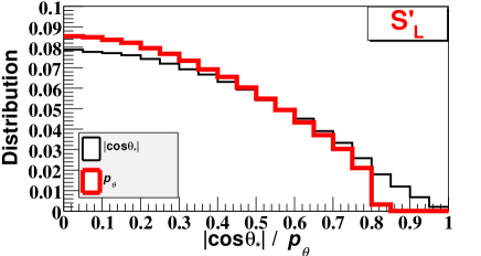
(a)

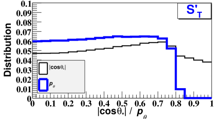
(b)

Figure 6: (a) Comparison between the normalized distributions of $p_{\theta}$ and $|\cos\theta_{*}|$ for the $\mathcal{S}_{L}^{\prime}$ event sample. (b) Same comparison for the $\mathcal{S}_{T}^{\prime}$ sample. The $|\cos\theta_{*}|$ distributions for the $\mathcal{S}_{L}^{\prime}$ and $\mathcal{S}_{T}^{\prime}$ samples are the same as those shown in Fig. 3, but here they are normalized to have unit area under the curve. The deviations between the $p_{\theta}$ and $|\cos\theta_{*}|$ distributions for each sample are due to the mismatch of the proxy variable with the true value of $|\cos\theta_{*}|$. The deviation is more apparent for transverse $W$ bosons only because of the significant number of events with $|\cos\,\theta_{*}|>0.8$, for which $p_{\theta}$ is a poor proxy.

In Fig. 6(a), we show the normalized distribution of $p_{\theta}$ for the pruned and tagged longitudinal $W$ sample $\mathcal{S}_{L}^{\prime}$. We also show, for comparison, the difference between this distribution and the normalized distribution of $|\cos\theta_{*}|$ for the same $\mathcal{S}_{L}^{\prime}$ sample. As explained above, there are two levels of distortion that alter our expectation of the distribution of the proxy variable as compared to the naive expectation of Eq. 6. The first effect is due to pruning and tagging cuts, and the second is the effect of distortion due to the imperfections of $p_{\theta}$ as a proxy for $|\cos\theta_{*}|$.

For the longitudinal $W$ boson, relatively few events have large $|\cos\theta_{*}|$ values. Pruning and tagging will mostly get rid of these events, and since $p_{\theta}$ tracks $|\cos\theta_{*}|$ well, the distribution of $p_{\theta}$ will look very similar to the parton level $1-|\cos\theta_{*}|^{2}$ distribution with a cut off at $|\cos\theta_{*}|\simeq 0.8$. Therefore the distortion of the $p_{\theta}$ distribution relative to the parton level $|\cos\theta_{*}|$ distribution in this case is minimal.

In Fig. 6(b), we show the same comparison for transverse $W$ bosons in the $\mathcal{S}_{T}^{\prime}$ sample. For the transverse $W$ bosons, there are a large number of events with $|\cos\theta_{*}|$ between 0.8 and 1.0. While pruning and tagging will get rid of a significant number of these, a non-negligible number of such events will survive the pruning and tagging cuts due to secondary radiation from the hard prong. These surviving events will have $p_{\theta}$ values which will spill over roughly uniformly into $p_{\theta}$ bins between 0.0 and 0.8. Thus, we see a significantly distorted distribution for $p_{\theta}$ as compared to $|\cos\theta_{*}|$, where the $p_{\theta}$ distribution is mostly flat up to 0.8 and then sharply drops to zero for larger values of $|\cos\theta_{*}|$.

Finally, in Fig. 7, we show a comparison of the $p_{\theta}$ distribution for the pruned and tagged samples $\mathcal{S}_{L}^{\prime}$ and $\mathcal{S}_{T}^{\prime}$. We see that despite the distortions away from the expected distributions for $|\cos\theta_{*}|$, the $p_{\theta}$ distributions are still characteristically distinct from each other.

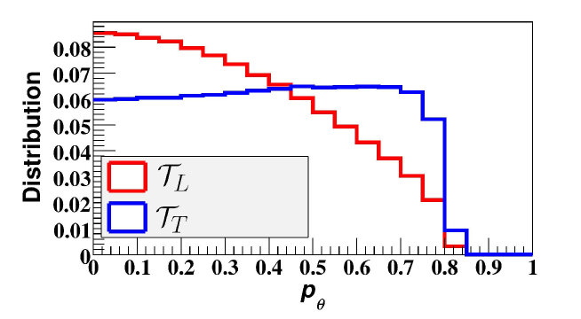
Figure 7: Having understood the normalized distributions of $p_{\theta}$ for the $\mathcal{S}_{L}^{\prime}$ and $\mathcal{S}_{T}^{\prime}$ samples, we can now define universal templates $\mathcal{T}_{L}$ and $\mathcal{T}_{T}$ for the proxy variable distributions, as shown in the figure. These templates can be used to extract $W$ boson polarization in a mixed sample.

We take the normalized distribution of $p_{\theta}$ for longitudinal $W$ bosons in the $\mathcal{S}_{L}^{\prime}$ sample and we take this to be a universal (production process independent) template for all longitudinal $W$ bosons which we will henceforth refer to as $\mathcal{T}_{L}$. Similarly, for the transverse $W$ bosons we can define, from the distribution of $p_{\theta}$ for the $\mathcal{S}_{T}^{\prime}$ sample, the universal template $\mathcal{T}_{T}$. A general distribution of $p_{\theta}$ for a mixed polarization sample of $W$ bosons can be fit to a linear combination of these templates to extract the polarization fractions.

4.5 Data-driven templates and calibration

If we were to directly use the templates of Fig. 7 to infer $W$ polarizations in experimental data, there is the possibility of drawing incorrect inferences because of limitations of either, the leading order approximation of partonic $W$ decays, or the Monte Carlo showering and hadronization procedure. Thus, it is important to develop templates analogous to the ones generated in simulation, directly from experimental data, rather than rely on simulations alone. A comparison between the data driven templates and the simulated ones would also provide an intriguing cross-check of the simulation itself.

One very interesting question that could be addressed by such a comparison, is whether the enhanced tagging rate for strongly-asymmetric $W$ decays (those with $|\cos\theta_{*}|>0.8$ at parton level), relative to the tagging rate for QCD jets is physical, or present only in Monte Carlo simulations. While the $|\cos\theta_{*}|$ variable is defined only at parton level, and thus is not physically observable, the effects of the tagging enhancement are also visible in the template functions, most directly illustrated in the transverse $W$ boson template in Fig. 6(b). The increase in events at low $p_{\theta}$ in particular, makes the shape of the $p_{\theta}$ distribution approximately flat for these low $p_{\theta}$ values, as compared to the parton level expectation for the slope of the $|\cos\theta_{*}|$ distribution which is noticeably positive in Fig. 6(b). This change in behaviour arises from the tagging of events that have $|\cos\theta_{*}|>0.8$ at parton level and should have been rejected as single prong events, but are tagged based on QCD radiation from the hard prong, and thus have reconstructed $p_{\theta}$ values which are distributed over $|\cos\theta_{*}|<0.8$. If the flat slope of the $p_{\theta}$ distribution is not observed in LHC data in transverse $W$ boson samples, it would indicate that some aspect of the modelling of decay products of heavy vector bosons in Pythia does not accurately describe the true physics of the situation.

Next, we address the question of how to construct samples of longitudinal and transverse $W$ bosons in experiments, which can be used to generate data-driven templates. To generate a transverse vector boson sample, we could use vector boson production in association with jets. Vector bosons produced off of effectively massless quarks are produced almost solely with transverse polarizations, and this process is common enough to provide a large sample for calibration. Developing such a template would directly probe the questions about the asymmetric $W$ decays discussed above.

Once we have a template for tagged transverse vector bosons, the longitudinal template could be derived from a mixed sample with a large known fraction of longitudinal $W$ bosons by subtracting the expected distribution of $p_{\theta}$ of the transverse $W$ bosons in the sample. A likely candidate process, where a significant number of longitudinal bosons are present, is Higgs production in association with a vector boson. This process has already been detected at the $5\sigma$ level with leptonic decays of the vector boson Aaboud:2018zhk ; Sirunyan:2018kst . With a high luminosity run at the LHC, we would have a huge sample of vector bosons from this process, which could be used to calibrate the templates. Diboson production also provides a sample for potential template construction, and one where there is already evidence for the presence of longitudinal $W$ polarizations Aaboud:2019gxl . The longitudinal polarization fraction of these samples can be determined by fitting distributions of kinematic variables in similar samples, but with leptonic decays of the vector bosons. The leptonic decay channels are well understood theoretically at high orders in electroweak couplings, and thus the polarization of these samples can be well determined and can then be used to infer the polarization of the corresponding hadronic decay event samples.

Thus, by the procedures outlined above, we can obtain purely data-driven templates for the $p_{\theta}$ distributions of longitudinal and transverse $W$ bosons, and we can also cross-check some of the features of the templates generated in the simulations.

5 Applications to polarization measurement at the LHC

In this section, we will discuss two applications of $W$ polarization measurement at the LHC, and we will demonstrate how the proxy variable $p_{\theta}$ can be used to make these measurements. First, we will show how to measure the polarization fraction of a mixed sample of hadronically-decaying longitudinal and transverse $W$ bosons taking VBS as a test case, and second, we will show that our technique can be used to identify the nature of a scalar/pseudo-scalar resonance decaying purely to $W$ bosons of a specific polarization.

5.1 Reconstructing the polarization of a mixed sample of $W$ bosons

Our strategy to measure the polarization fraction of a mixed sample of $W$ bosons is to construct the distribution of the proxy variable $p_{\theta}$ for tagged $W$ bosons in the mixed sample, and then to fit this distribution to a linear combination of the templates $\mathcal{T}_{L}$ and $\mathcal{T}_{T}$. In a mixed sample of $W$ bosons, event tagging selection cuts would distort the polarization fraction due to the different tagging efficiencies of longitudinal and transverse $W$ bosons . If the longitudinal polarization fraction in a sample is denoted as $f_{L}$ before the tagging cuts are applied, then the polarization fraction after tagging cuts are applied (which we denote as $f_{L}^{\prime}$) will be given by,

$$f_{L}^{\prime}=\frac{\epsilon_{L}f_{L}}{\epsilon_{L}f_{L}+\epsilon_{T}(1-f_{L})}.$$ (9)

Here, $\epsilon_{L}$ and $\epsilon_{T}$ are the tagging efficiencies for longitudinal and transverse $W$ bosons respectively. Thus, if we reconstruct $f_{L}^{\prime}$, we can invert the above equation using the known tagging efficiencies to infer the value of $f_{L}$ of the original mixed sample without tagging cuts.

5.1.1 Polarization Reconstruction in semi-leptonic VBS

As a test case, we will study a mixed sample of $W$ boson polarizations in the semi-leptonic VBS channel, $pp\rightarrow W^{-}W^{+}jj\rightarrow\ell^{-}\overline{\nu}_{\ell}jjjj$ in the Standard Model, where the $W^{+}$ boson decays hadronically and the $W^{-}$ decays leptonically ($\ell$ denotes either electrons or muons). We will attempt to reconstruct the longitudinal and transverse polarization fractions of the $W^{+}$ boson in these events.

This process is very important for testing unitarity of longitudinal $W$ boson scattering in the Standard Model. If the Higgs boson discovered in 2012 Aad:2012tfa ; Chatrchyan:2012ufa does not have the exact couplings to gauge bosons as predicted in the SM then we would expect that unitarity of longitudinal $W$-boson scattering must be restored by additional new resonances exchanged in longitudinal VBS, possibly at energies inaccessible to the LHC. Thus, disentangling the polarization fractions would be critical for precision tests of the SM and unitarity restoration in VBS.

As mentioned in the introduction, previous studies have used the angular distribution of the leptonic $W$ to study its polarization. However, the advantage of measuring the polarization of the hadronic $W$ is that it allows us to simultaneously measure the polarization of both $W$ bosons in VBS events. Note that this can not be done in the fully leptonic channel, because of kinematic reconstruction ambiguities.

We have generated events for the process: $pp\rightarrow W^{-}W^{+}jj\rightarrow\ell^{-}\bar{\nu_{\ell}}jjjj$ in MadGraph at 13 TeV center-of-mass energy, which includes the VBS processes of interest, but also a large number of irreducible SM background channels. These events are further passed to Pythia 8, where we perform a parton shower and hadronization simulation. The resulting particles in the event (other than neutrinos and the hardest lepton) are clustered into jets using the FastJet package. We use the Cambridge-Aachen (CA) clustering algorithm with jet size parameter $R_{0}=1.0$ for all the jets in the event. We also prune our jets using the same pruning parameters, $z_{\textrm{cut}}=0.1$ and $\Delta R_{\textrm{cut}}=0.25$, that we used in Sec. 4.1 for our calibration samples. As in our calibration studies, we have not performed a detector simulation.

We then identify the leading $p_{T}$ jet which passes our tagging cuts as the hadronic $W$ boson. In order to select boosted $W$ bosons, but still maintain reasonable statistics, we keep events where the tagged jet has a $p_{T}>400$ GeV. After this, the two leading $p_{T}$ jets (excluding the one identified as the $W$) are identified as the associated jets in VBS and are subjected to standard VBS selections cuts, namely a rapidity gap cut $|\Delta\eta_{jj}|>4.0$ and a large invariant mass cut $M_{jj}>200$ GeV to select high center-of-mass-energy events. In order to increase the longitudinal polarization fraction of the sample, we also found it useful to impose a lower rapidity cut on the forward jets to select events with $2<|\eta|<4.7$, where the upper rapidity cut is as usual limited by detector coverage.

The full set of selection and tagging cuts imposed on our event sample are listed in Table 1. In our simulation, we have imposed the basic kinematic cuts and associated jet cuts at the parton level in Madgraph and once again on the hadron level output from Pythia.

Basic selection cuts
$p_{T}$ of the lepton	${p^{\ell}_{T}>25}$ GeV
$\eta$ of the lepton	$\mathrm{|\eta^{\ell}|<2.5}$
$p_{T}$ of the jets	${p^{j}_{T}>30}$ GeV
Associated jet cuts
Pseudo-rapidity gap between the associated forward jets	$|\Delta\eta_{jj}|>4.0$
Invariant mass of the associated jets	$M_{jj}>200$ GeV
$\eta$ of the forward jets	$2<\mathrm{|\eta_{j}|<4.7}$
Hadronic $W^{+}$ tagging and selection cuts
Fat-jet mass cut	60 GeV $<$ $M_{j}$ $<$ 100 GeV
Mass-drop cut	$\mu^{\mathrm{cut}}<0.25$, $y^{\mathrm{cut}}<0.09$
$N$-Subjettines Ratio	$\tau_{2}/\tau_{1}<0.3$
$p_{T}$ of the tagged jet	$p^{j}_{T}>400$ GeV

Table 1: The full set of selection cuts that we impose on our VBS events. All jets are clustered using the CA algorithm with $R_{0}=1.0$. The highest $p_{T}$ jet that passes the tagging cuts is identified as the $W^{+}$ boson. The next two leading $p_{T}$ jets are identified as the associated jets and subjected to the associated jet cuts.

Monte-Carlo truth information (pre-tagging): For each event, we can extract the angle $|\cos\theta_{*}|$ between the hadronic $W$ decay partons using the event record generated by MadGraph. We then use the partonic angular distribution of the $W$ decay products obtained from MadGraph to construct the angle $|\cos\theta_{*}|$ and fit it to the expression in Eq. 6 to extract the polarization fraction of the $W$ bosons before tagging. Using this procedure, we find that the longitudinal polarization fraction $f_{L}=0.12$ before hadron level kinematic and tagging cuts are applied, but after parton level kinematic cuts are applied. Since we can also compute the tagging efficiencies of $W$ bosons of different helicities using our templates, we can find the expected longitudinal polarization fraction after tagging cuts are applied as $f_{L}^{\prime}=0.15$ using Eq. 9. Here we have assumed that the kinematic cuts which have been reapplied at the hadron level do not further preferentially select for $W$ bosons of a particular polarization, once the kinematic cuts have been applied at the parton level.

Expected number of events: The total Standard Model cross-section after all cuts are imposed is 0.048 fb. This is a very small cross-section and it makes the study of $WW$ scattering very challenging until we reach a very high integrated luminosity at the LHC.

With 3 ab^-1 of data that might be expected at the high-luminosity LHC (HL-LHC) Apollinari:2017cqg , we would thus expect to get $\sim$ 144 events. If we also take into account a similar VBS process involving the $W^{-}$ decaying hadronically and the $W^{+}$ decaying leptonically, we might expect to double our statistics to about $\sim$ 288 events.

In what follows, we will take several pseudo-experiment benchmark samples of 288 SM-like events post-VBS selection and hadronic $W$-tagging cuts corresponding to $\sim$ 3 ab^-1 integrated luminosity at the LHC. We will use these samples to assess our ability to measure the polarization fraction of hadronic $W$ bosons in VBS.

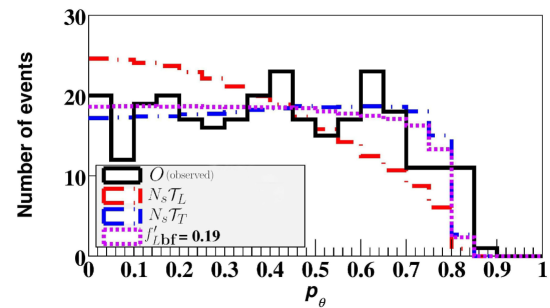
Figure 8: $p_{\theta}$ distribution for a particular benchmark sample of $N_{s}=288$ VBS events, corresponding to $\sim$ 3 ab^-1 of luminosity, and after all selection and tagging cuts are applied (black curve). The best-fit linear combination of templates with longitudinal $W$ fraction $f^{\prime}_{L\textrm{{bf}}}=0.19$ is shown with the magenta dotted curve. Also shown are the longitudinal and transverse templates ($\mathcal{T}_{L}$ and $\mathcal{T}_{T}$) rescaled to $N_{s}$ events.

Reconstructing the polarization fraction in hadronic $W$ decays We consider a particular sample of $N_{s}=288$ events which pass our VBS forward jet selection cuts and hadronic $W$ tagging cuts. For each of these events we construct the $p_{\theta}$ value of the tagged $W$ jet by decomposing it into two subjets and finding the energy difference between the subjets as described in Sec. 3. We then construct a distribution of $p_{\theta}$ values with 20 bins between 0 and 1 which we denote as $O$ (or observed), and fit it to a linear combination of the normalized templates for longitudinal ($\mathcal{T}_{L}$) and transverse ($\mathcal{T}_{T}$) $W$ bosons, which we rescale to the number of events $N_{s}$. Thus, we are parameterizing our fit to the distribution of $p_{\theta}$ as $\frac{dN}{dp_{\theta}}=N_{s}(f_{L}^{\prime}\mathcal{T}_{L}+\left(1-f_{L}^{\prime})\mathcal{T}_{T}\right)$, where $f_{L}^{\prime}$ is the longitudinal polarization fraction that we are fitting for. We show a distribution of the reconstructed $p_{\theta}$ values along with the rescaled templates in Fig. 8.

To obtain the best-fit parameter $f_{L}^{\prime}$ and its uncertainty, we have performed a $\chi^{2}$ test. The $\chi^{2}$ test-statistic with one parameter $f_{L}^{\prime}$ is given by,

$$\chi^{2}(f_{L}^{\prime})=\sum_{i=1}^{B}\frac{\left(O_{i}-N_{s}(f_{L}^{\prime}{\mathcal{T}_{L}}_{i}+(1-f_{L}^{\prime}){\mathcal{T}_{T}}_{i})\right)^{2}}{\sigma_{i}^{2}}$$ (10)

where, $O_{i}$ are the observed number of signal events in the $i^{th}$ bin, ${\mathcal{T}_{L}}_{i}$ is the value of the longitudinal $W$ boson template in the $i^{th}$ bin and ${\mathcal{T}_{T}}_{i}$ is the value of the transverse $W$ boson template in the $i^{th}$ bin. We assume Poissonian fluctuations in the predicted number of events and therefore we take $\sigma_{i}^{2}=N_{s}(f_{L}^{\prime}{\mathcal{T}_{L}}_{i}+(1-f_{L}^{\prime}){\mathcal{T}_{T}}_{i})$. We minimize the $\chi^{2}$ value over values of $f_{L}^{\prime}$ in the restricted range of 0 to 1. Here, $B$ denotes the number of bins to be summed over. While we have partitioned our histogram into 20 bins, only the first 16 bins are populated for the process under consideration. Hence, we will set $B=16$ in our definition of $\chi^{2}$.

The distribution of $\chi^{2}$ as a function of $f_{L}^{\prime}$ is shown in Fig. 9. The $\chi^{2}$ value is minimized for the best-fit value $f^{\prime}_{L\textrm{{bf}}}=0.19$ and the fit is quite good, as we obtain a value of $\chi^{2}$ per degree of freedom of 0.6 at the minimum. We can also find the 1-$\sigma$ uncertainty on the best-fit parameter by considering the range of parameters about the minimum with $\Delta\chi^{2}=1$ and we obtain the range $f_{L}^{\prime}\in[0.00,0.38]$. At the 2-$\sigma$ level, the upper value of allowed $f_{L}^{\prime}$ is 0.56.

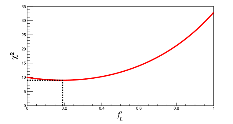
Figure 9: $\chi^{2}$ distribution as a function of the longitudinal polarization fraction $f_{L}^{\prime}$ for fits to the pseudo-experiment data shown in Fig. 8. We obtain a best-fit value of $f^{\prime}_{L\textrm{{bf}}}=0.19$ with a 1-$\sigma$ range between $[0.00,0.38]$, which is consistent with our expectation of $0.15$ from Monte-Carlo truth information about the longitudinal polarization fraction. The fit is quite good at the minimum with a $\chi^{2}$ per degree of freedom of 0.6.

The results shown above are for one pseudo-experiment, i.e. one realization of 288 events simulated at the LHC. We have performed multiple pseudo-experiments by resimulating multiple times and fitting for the value of $f_{L}^{\prime}$ and searching for its uncertainty in each pseudo-experiment. If we average the results over the $\sim$ 100 pseudo-experiments that we have generated, we find an average best-fit $f_{L}^{\prime}=0.19$ with an average 1-$\sigma$ range between [0.07, 0.36], and at the 2-$\sigma$ level we find a range between [0.02 , 0.52].

In order to determine whether we have reconstructed the polarization fraction accurately, we can compare this result to the Monte-Carlo truth information from MadGraph. Using the truth information on $W$ helicities obtained from MadGraph, we had argued that the expected polarization fraction $f_{L}^{\prime}=0.15$, which is in agreement (within the expected experimental uncertainties) with the value that we have found by using the reconstructed $p_{\theta}$ distribution. However, in our full Monte-Carlo event sample involving many pseudo-experiments, we see that the average best-fit value of $f_{L}^{\prime}=0.19$ that we have obtained is slightly larger than what we expect from the parton level expectation (appropriately corrected using the tagging efficiencies as in Eq. 9) of $f_{L}^{\prime}=0.15$.

The reason for this mild discrepancy is that the efficiencies we have used in Eq. 9 only take into account the different tagging efficiencies of longitudinal and transverse $W$ bosons, but they do not take into account kinematic selection efficiencies for different $W$ boson helicities at the hadron level. As we mentioned earlier, we have imposed the basic kinematic selection cuts and associated jet cuts at both the parton and hadron level. We find an approximate 50% reduction in the number of hadronic events due to the tagging efficiencies of $W$ bosons of any helicity, however, we also find a further 50% reduction in the number of hadronic events due to the kinematic cuts which are imposed once again at the hadron level. We have confirmed that these kinematic cuts (reimposed at the hadron level) preferentially select for longitudinal $W$ bosons by studying the corresponding parton level $|\cos\theta_{*}|$ distribution after imposing all hadron level kinematic cuts but before imposing the tagging cuts, thus altering our expectation of Eq. 9. We discuss possible reasons for this preference below.

Even after imposing the kinematic cuts at parton level, our event sample has contributions from sub-processes which have a different parton level event topology than that of VBS. These non-VBS processes are dominated by transverse $W$ bosons and have a different color structure from the VBS events. Thus, the radiation and shower pattern of these events at hadron level would be different from the VBS events, and it is possible that a larger fraction of these are cut, relative to the fraction cut in VBS events, once we reimpose the cuts at the hadron level. Thus, reimposing the cuts at the hadron level could preferentially select for longitudinal $W$ bosons.

Thus, we have seen that we are able to reconstruct the polarization fraction $f_{L}^{\prime}$ of the hadronic $W$ bosons in VBS by using our proxy variable $p_{\theta}$. Given an experimental event sample with a number of selection cuts, if we want to infer the $W$ boson polarization $f_{L}$ before the cuts are imposed, we can invert Eq. 9 with efficiencies $\epsilon_{L}$, $\epsilon_{T}$ only taking into account the tagging efficiencies for different $W$ boson polarizations. However, for a more precise determination of $f_{L}$ assuming large enough statistics, we would also need to understand how kinematic cuts on different event topologies select for different $W$ boson polarizations at the hadron level and determine the corresponding efficiencies.

5.2 Resonance discrimination

As another application of our technique, we take the example of a beyond Standard Model (BSM) resonance decaying to purely longitudinal or transverse $W$ bosons (for e.g. via a scalar or pseudo-scalar resonance, respectively). If such a resonance is discovered, then our technique can be used to probe the polarization of the $W$ bosons and hence learn about the nature of the resonance.

The resonance events are expected to have a $p_{\theta}$ distribution that would look exactly like either the template $\mathcal{T}_{L}$ or $\mathcal{T}_{T}$ rescaled to the number of resonance events $N$. We can estimate the number of events required to discriminate between the purely longitudinal and purely transverse $W$ boson decays of the new resonance as follows:

1. For concreteness, let us take the case that the resonance decays to purely longitudinal $W$ bosons. We will assume that the decays are semi-leptonic, so that one of the $W$s decays to hadrons and the other to leptons. We will analyze the polarization of the hadronic $W$ to characterize the resonance.

2. In an experimental analysis, if we took the null hypothesis to be that the resonance decays to purely transverse $W$ bosons, we could exclude this hypothesis with sufficient data. For a given observed $p_{\theta}$ distribution, we can define a log-likelihood ratio test statistic $q\equiv-2\log{\frac{\mathcal{L}_{1}}{\mathcal{L}_{0}}}$, where $\mathcal{L}_{0}$ is the likelihood for the null hypothesis (transverse $W$) and $\mathcal{L}_{1}$ is the likelihood for the alternate hypothesis (longitudinal $W$). We use reduced Poissonian likelihoods defined as,

   $$\log{\mathcal{L}}=\sum_{i}(-\log P_{i}+O_{i}\log P_{i})$$ (11)

   where $O_{i}$ is the observed number of events and $P_{i}$ is the predicted number of events in each bin, i.e. $P_{i}=N{\mathcal{T}_{L}}_{i}$ for longitudinal $W$ bosons and $P_{i}=N{\mathcal{T}_{T}}_{i}$ for transverse $W$ bosons, and $N$ is the total number of events. We assume the same number of $p_{\theta}$ bins for analysis (16) as before.

3. For a given number of events $N$, we can then calculate the expected test statistic under the assumption that the data corresponds to statistical fluctuations of purely longitudinal $W$ boson resonances. We take a simple assumption of independent Poissonian statistical fluctuations in each $p_{\theta}$ bin.

4. For a given value of $N$, we can then calculate the expected exclusion $p$-value corresponding to this average test statistic. We can then ask, how many events are required to rule out the null hypothesis at the 2-$\sigma$ (95%) confidence level.

5. We find that with just 24 events we can rule out the transverse $W$ boson hypothesis.

Similarly, if we take purely longitudinal $W$ bosons as our null hypothesis, and the resonance decays to purely transverse $W$ bosons, the null hypothesis can be ruled out at the 95% confidence level with just 19 events. Both these values are calculated with the background-free assumption, as a narrow resonance would lead to a small diboson invariant mass window, in which we would have a relatively low SM rate. A dedicated study would be needed to assess optimal cuts and backgrounds for a given resonance mass, width, and cross-section.

Thus, for a BSM scalar or pseudo-scalar resonance with relatively little background, we find that with around 20 events, we could use our technique to measure the $W$ boson polarization in hadronic decays and identify the parity of the resonance.

6 Limitations of our study

While the outlook for measuring $W$ boson polarization in hadronic decays using the proxy variable that we have proposed seems promising with high enough luminosity, there are several limitations of our preliminary study that need to be improved upon in order to confirm this expectation. We discuss each of these in turn below:

Backgrounds: Any process involving hadronic $W$ bosons will have irreducible QCD backgrounds that remain despite kinematic cuts. The amount of background would depend on the kinematic cuts and specific event signature and topology that we are studying. For semi-leptonic $WW$ scattering for example, the QCD background processes would mainly be associated with $W$ + jets or $Z$ + jets (with one lepton from $Z$ decay either missed or misidentified as a jet). While forward jet cuts and tagging cuts will reduce a significant amount of such background, a detailed study is needed to estimate the amount of background contamination.

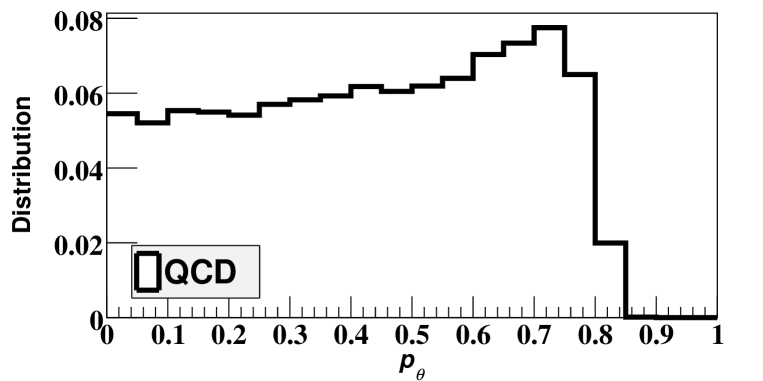
Figure 10: Normalized $p_{\theta}$ distribution for a sample of QCD jets that pass the $W$ boson tagging cuts. This distribution is characteristically different from $W$ bosons because of the preference for higher $p_{\theta}$, which is expected due to a preference for soft radiation from parton splitting that leads to asymmetric prongs within the jet. This can be used to define a background template $\mathcal{T}_{B}$. One could then try to fit the $p_{\theta}$ distribution in a $W$ boson sample with QCD background to extract the QCD contribution and thus get a better estimate of the $W$ polarization fraction in the sample.

The QCD jets that pass our tagging cuts would typically be produced from a parton which undergoes splitting. Since the splitting in QCD prefers soft and collinear radiation, it will characteristically lead to a preferentially asymmetric splitting of the prongs. This would lead to a $p_{\theta}$ distribution that prefers higher values of $p_{\theta}$ ($\simeq 1$). While our choice of pruning parameters and tagging cuts would once again remove events with $p_{\theta}\gtrsim 0.8$, the distribution continues to show a preference for high $p_{\theta}$ values. The normalized distribution of $p_{\theta}$ for a sample of QCD jets that pass the $W$ boson tagging cuts is shown in Fig. 10. In principle, we could model this contribution to the overall $p_{\theta}$ distribution of signal plus background. If we identify this template for background events as $\mathcal{T}_{B}$, then we could fit our overall $p_{\theta}$ distribution to a linear combination of $\mathcal{T}_{L}$, $\mathcal{T}_{T}$ and $\mathcal{T}_{B}$ as,

$$\frac{dN}{dp_{\theta}}=N\left(f_{L}^{\prime}\mathcal{T}_{L}+f_{T}^{\prime}\mathcal{T}_{T}+f_{B}^{\prime}\mathcal{T}_{B}\right).$$ (12)

Here $N$ is the total number of events in the sample that we are studying, including both signal and background and $f_{L}^{\prime}$, $f_{T}^{\prime}$ and $f_{B}^{\prime}$ are fit parameters that we identify as the fraction of longitudinal $W$ bosons, transverse $W$ bosons and background events in the sample respectively. These fit parameters are subject to the constraint $f_{L}^{\prime}+f_{T}^{\prime}+f_{B}^{\prime}=1$.

In practice, since the background template bears some similarity to the transverse $W$ boson template, we expect that there will be a slight degeneracy in the fit parameters $f_{T}^{\prime}$ and $f_{B}^{\prime}$ which will make identification of the transverse $W$ polarization fraction harder, depending on the level of background contamination.

Pile-up: Our study also did not simulate the effect of pile-up which will be a significant issue at higher instantaneous luminosities. Various techniques such as vertex reconstruction could help us in pile-up subtraction. Moreover, the pruning algorithms that we are using will help in removal of some of the soft and wide-angle contamination. However, a more detailed study is needed to assess the effects of pile-up on the distribution of the proxy variable $p_{\theta}$ that we have constructed.

7 Conclusions

There are a number of SM and beyond Standard Model processes which lead to polarized $W$ boson production at high $p_{T}$. In this work we have proposed a technique to measure the polarization fraction of boosted-hadronically decaying $W$ bosons at the LHC. Such a measurement would be useful for increasing statistical sensitivity to $W$ polarization and will also allow us to simultaneously measure the polarization of both final state $W$ bosons in vector boson scattering processes.

We found that at the parton level, the distribution of the decay polar angle $|\cos\theta_{*}|$ allows us to extract the longitudinal vs transverse polarization fraction. We then found a proxy variable $p_{\theta}$, constructed from jet substructure observables, that tracks the parton level variable extremely well. We have demonstrated how to construct templates of the distribution of $p_{\theta}$ from simulated samples of pure longitudinal and transverse $W$ bosons and we discussed the intuitive reasons for the distortions in the distribution of this proxy variable as compared to the parton level $|\cos\theta_{*}|$ distribution.

Once we constructed our templates, we showed how we could use them to accurately reconstruct the polarization fraction of a mixed sample of $W$ bosons at the LHC. Taking as an example the important process of semi-leptonic $WW$ scattering, we showed how to measure the polarization fraction of the hadronically decaying $W$ boson by constructing the $p_{\theta}$ distribution and fitting it to a linear combination of our templates. While the cross-section for high energy VBS scattering is low, especially once VBS selection and hadronic $W$ tagging cuts are imposed, we showed that with 3 ab^-1 of integrated luminosity at the HL-LHC, we could potentially reconstruct the observed longitudinal polarization fraction to within a $\pm 0.15$ uncertainty at the 1-$\sigma$ level.

We have also discussed another use potential application of our polarization measurement technique to characterize new scalar/pseudo-scalar resonances that decay purely to either longitudinal or transverse $W$ bosons. We have found that with around 20 events, our technique would be able to identify whether the resonance is a scalar or pseudo-scalar by measuring the polarization of the $W$ bosons.

Our study is intended to motivate a more detailed application of our technique to a realistic collider environment where pile-up and QCD background processes need to be taken into account. We have also suggested a technique by which background processes may be dealt with, by modelling the distribution of the background $p_{\theta}$ distribution (and fitting for it simultaneously while fitting for the longitudinal and transverse polarization fractions), and we have shown that this is characteristically different from the longitudinal or transverse $W$ boson distributions.

In summary, we hope that the technique proposed in this work will prove to be a valuable tool to the experimental collider physics community to measure hadronic $W$ boson polarizations.

Appendix A Model used to generate pure longitudinal and transverse $W$ polarizations

To generate our calibration samples of purely longitudinal or transverse $W$ bosons, we use specific interaction Lagrangians implemented in FeynRules Christensen:2008py .

To generate longitudinal $W$ bosons, we introduce a fictitious scalar particle $\phi_{s}$ with Higgs-like couplings to $W$ bosons and gluons,

$$\mathcal{L}_{\textrm{\tiny{s}}}=c_{1}\phi_{s}W^{\mu}W_{\mu}+c_{2}\phi_{s}G^{\mu\nu}G_{\mu\nu},$$ (13)

where $c_{1}$ and $c_{2}$ are coupling constants. We then generate events with the process $pp\rightarrow\phi_{s}\rightarrow W^{+}W^{-}\rightarrow jjjj$ in MadGraph, where the production of $\phi_{s}$ proceeds through gluon fusion. The interaction of the scalar with $W$ bosons is through a non-gauge invariant, renormalizable term. Even if we choose $\phi_{s}$ to be the SM Higgs boson, by specifically forcing the process to go through an $s$-channel Higgs in MadGraph, we are choosing a non-gauge invariant set of diagrams. However, for our purposes this is exactly what is needed, since it picks out longitudinal $W$ bosons at high energies by the Goldstone equivalence theorem. There will be a small admixture of transverse $W$ bosons in the sample, but they will be suppressed by a fraction $\sim m_{W}^{4}/E^{4}\simeq 10^{-4}$ for $W$ bosons with energies of order 800 GeV - 1 TeV.

To generate transverse $W$ bosons, we use non-renormalizable dimension-5 interaction terms for a fictitious pseudo-scalar field $\phi_{ps}$ which couples to both $W$s and gluons,

$$\mathcal{L}_{\textrm{\tiny{ps}}}=c^{\prime}_{1}\phi_{ps}W^{\mu\nu}\widetilde{W}_{\mu\nu}+c^{\prime}_{2}\phi_{ps}G^{\mu\nu}\widetilde{G}_{\mu\nu}.$$ (14)

We then generate events with the process $pp\rightarrow\phi_{ps}\rightarrow W^{+}W^{-}\rightarrow jjjj$ in MadGraph, where production once again proceeds through gluon fusion. The amplitude for $W$ boson production from the pseudo-scalar vertex is of the form $\mathcal{M}\propto\epsilon^{\mu\nu\rho\sigma}k^{1}_{\mu}\epsilon^{1}_{\nu}k^{2}_{\rho}\epsilon^{2}_{\sigma}$, where $\epsilon^{\mu\nu\rho\sigma}$ is the fully-antisymmetric tensor and $k^{i}$, $\epsilon^{i}$ denote the four-momentum and polarization vector for the $i$-th $W$ boson in the event. We can evaluate this expression in the center-of-momentum frame, where the $W$ bosons are back-to-back and, without loss of generality, moving along the $z$-axis. Since, the $k$ vectors have non-zero time-like and $z$-components only, we obtain non-zero amplitudes only when both polarization vectors are transverse.

Although the arguments we have given for the expected purity of the polarization fractions in these models is valid in the center-of-momentum frame of the partons, we have checked, by fitting the $\cos\theta_{*}$ distribution, that the polarization fraction is the same in the lab-frame of the simulated $pp$ collision.

Note that for both interaction Lagrangians, the mass of the scalar/pseudo-scalar and the choice of coupling constants are irrelevant for our purposes. However, we choose the masses of the fictitious particles to be less than $2m_{W}$, so that the resonances are off-shell and the $W$ bosons are produced with a kinematic phase-space distribution similar to that of signal events associated with a typical hard process, such as VBS.

References

- (1) ATLAS Collaboration Collaboration, G. Aad et. al., Observation of a new particle in the search for the Standard Model Higgs boson with the ATLAS detector at the LHC, Phys.Lett. B716 (2012) 1–29, [arXiv:1207.7214].
- (2) CMS Collaboration Collaboration, S. Chatrchyan et. al., Observation of a new boson at a mass of 125 GeV with the CMS experiment at the LHC, Phys.Lett. B716 (2012) 30–61, [arXiv:1207.7235].
- (3) D. E. Morrissey, T. Plehn, and T. M. Tait, Physics searches at the LHC, Phys.Rept. 515 (2012) 1–113, [arXiv:0912.3259].
- (4) M. Farina, D. Pappadopulo, and A. Strumia, A modified naturalness principle and its experimental tests, JHEP 1308 (2013) 022, [arXiv:1303.7244].
- (5) J. L. Feng, Naturalness and the Status of Supersymmetry, Ann.Rev.Nucl.Part.Sci. 63 (2013) 351–382, [arXiv:1302.6587].
- (6) A. de Gouvea, D. Hernandez, and T. M. P. Tait, Criteria for Natural Hierarchies, arXiv:1402.2658.
- (7) S. P. Martin, A Supersymmetry primer, hep-ph/9709356. [Adv. Ser. Direct. High Energy Phys.18,1(1998)].
- (8) C. Csáki, S. Lombardo, and O. Telem, TASI Lectures on Non-supersymmetric BSM Models, in Proceedings, Anticipating the Next Discoveries in Particle Physics (TASI 2016), pp. 501–570, WSP, WSP, 2018. arXiv:1811.0427.
- (9) W. Kilian, T. Ohl, J. Reuter, and M. Sekulla, High-Energy Vector Boson Scattering after the Higgs Discovery, Phys. Rev. D91 (2015) 096007, [arXiv:1408.6207].
- (10) W. Kilian, T. Ohl, J. Reuter, and M. Sekulla, Resonances at the LHC beyond the Higgs boson: The scalar/tensor case, Phys. Rev. D93 (2016), no. 3 036004, [arXiv:1511.0002].
- (11) CMS Collaboration, S. Chatrchyan et. al., Measurement of the Polarization of W Bosons with Large Transverse Momenta in W+Jets Events at the LHC, Phys. Rev. Lett. 107 (2011) 021802, [arXiv:1104.3829].
- (12) ATLAS Collaboration, G. Aad et. al., Measurement of the W boson polarization in top quark decays with the ATLAS detector, JHEP 06 (2012) 088, [arXiv:1205.2484].
- (13) T. Han, D. Krohn, L.-T. Wang, and W. Zhu, New Physics Signals in Longitudinal Gauge Boson Scattering at the LHC, JHEP 1003 (2010) 082, [arXiv:0911.3656].
- (14) A. Ballestrero, E. Maina, and G. Pelliccioli, Polarized vector boson scattering in the fully leptonic WZ and ZZ channels at the LHC, Submitted to: J. High Energy Phys. (2019) [arXiv:1907.0472].
- (15) J. Brehmer, Polarised WW Scattering at the LHC, Master’s thesis, U. Heidelberg, ITP, 2014.
- (16) J. Thaler and K. Van Tilburg, Identifying Boosted Objects with N-subjettiness, JHEP 03 (2011) 015, [arXiv:1011.2268].
- (17) C. Englert, C. Hackstein, and M. Spannowsky, Measuring spin and CP from semi-hadronic ZZ decays using jet substructure, Phys.Rev. D82 (2010) 114024, [arXiv:1010.0676].
- (18) M. R. Buckley, H. Murayama, W. Klemm, and V. Rentala, Discriminating spin through quantum interference, Phys.Rev. D78 (2008) 014028, [arXiv:0711.0364].
- (19) M. R. Buckley, B. Heinemann, W. Klemm, and H. Murayama, Quantum Interference Effects Among Helicities at LEP-II and Tevatron, Phys.Rev. D77 (2008) 113017, [arXiv:0804.0476].
- (20) A. Ballestrero, E. Maina, and G. Pelliccioli, boson polarization in vector boson scattering at the LHC, JHEP 03 (2018) 170, [arXiv:1710.0933].
- (21) E. Mirkes and J. Ohnemus, and polarization effects in hadronic collisions, Phys. Rev. D 50 (1994) 5692–5703, [hep-ph/9406381].
- (22) W. Stirling and E. Vryonidou, Electroweak gauge boson polarisation at the LHC, JHEP 07 (2012) 124, [arXiv:1204.6427].
- (23) A. Belyaev and D. Ross, What Does the CMS Measurement of W-polarization Tell Us about the Underlying Theory of the Coupling of W-Bosons to Matter?, JHEP 08 (2013) 120, [arXiv:1303.3297].
- (24) Y. L. Dokshitzer, G. D. Leder, S. Moretti, and B. R. Webber, Better jet clustering algorithms, JHEP 08 (1997) 001, [hep-ph/9707323].
- (25) M. Wobisch and T. Wengler, Hadronization corrections to jet cross-sections in deep inelastic scattering, in Monte Carlo generators for HERA physics. Proceedings, Workshop, Hamburg, Germany, 1998-1999, pp. 270–279, 1998. hep-ph/9907280.
- (26) S. Catani, Y. L. Dokshitzer, M. H. Seymour, and B. R. Webber, Longitudinally invariant clustering algorithms for hadron hadron collisions, Nucl. Phys. B406 (1993) 187–224.
- (27) S. D. Ellis and D. E. Soper, Successive combination jet algorithm for hadron collisions, Phys. Rev. D48 (1993) 3160–3166, [hep-ph/9305266].
- (28) S. P. Lloyd, Least squares quantization in pcm, IEEE Transactions on Information Theory 28 (1982) 129–137.
- (29) J. Alwall, R. Frederix, S. Frixione, V. Hirschi, F. Maltoni, O. Mattelaer, H. S. Shao, T. Stelzer, P. Torrielli, and M. Zaro, The automated computation of tree-level and next-to-leading order differential cross sections, and their matching to parton shower simulations, JHEP 07 (2014) 079, [arXiv:1405.0301].
- (30) T. Sjostrand, S. Mrenna, and P. Z. Skands, PYTHIA 6.4 Physics and Manual, JHEP 05 (2006) 026, [hep-ph/0603175].
- (31) T. Sjostrand, S. Mrenna, and P. Z. Skands, A Brief Introduction to PYTHIA 8.1, Comput. Phys. Commun. 178 (2008) 852–867, [arXiv:0710.3820].
- (32) M. Cacciari, G. P. Salam, and G. Soyez, FastJet User Manual, Eur. Phys. J. C72 (2012) 1896, [arXiv:1111.6097].
- (33) S. D. Ellis, C. K. Vermilion, and J. R. Walsh, Techniques for improved heavy particle searches with jet substructure, Phys. Rev. D80 (2009) 051501, [arXiv:0903.5081].
- (34) J. M. Butterworth, A. R. Davison, M. Rubin, and G. P. Salam, Jet substructure as a new Higgs search channel at the LHC, Phys. Rev. Lett. 100 (2008) 242001, [arXiv:0802.2470].
- (35) CMS Collaboration, C. Collaboration, Pileup Removal Algorithms, .
- (36) ATLAS Collaboration, Jet energy scale and its systematic uncertainty in proton-proton collisions at sqrt(s)=7 TeV with ATLAS 2011 data, .
- (37) CMS Collaboration, V. Khachatryan et. al., Jet energy scale and resolution in the CMS experiment in pp collisions at 8 TeV, JINST 12 (2017), no. 02 P02014, [arXiv:1607.0366].
- (38) ATLAS Collaboration, M. Aaboud et. al., Observation of decays and production with the ATLAS detector, Phys. Lett. B 786 (2018) 59–86, [arXiv:1808.0823].
- (39) CMS Collaboration, A. M. Sirunyan et. al., Observation of Higgs boson decay to bottom quarks, Phys. Rev. Lett. 121 (2018), no. 12 121801, [arXiv:1808.0824].
- (40) ATLAS Collaboration, M. Aaboud et. al., Measurement of production cross sections and gauge boson polarisation in collisions at TeV with the ATLAS detector, Eur. Phys. J. C 79 (2019), no. 6 535, [arXiv:1902.0575].
- (41) ATLAS Collaboration, G. Aad et. al., Combined measurements of Higgs boson production and decay using up to fb-1 of proton-proton collision data at 13 TeV collected with the ATLAS experiment, Phys. Rev. D 101 (2020), no. 1 012002, [arXiv:1909.0284].
- (42) CMS Collaboration, A. M. Sirunyan et. al., Combined measurements of Higgs boson couplings in proton–proton collisions at , Eur. Phys. J. C79 (2019), no. 5 421, [arXiv:1809.1073].
- (43) G. Apollinari, O. Brüning, T. Nakamoto, and L. Rossi, High Luminosity Large Hadron Collider HL-LHC, CERN Yellow Rep. (2015), no. 5 1–19, [arXiv:1705.0883].
- (44) N. D. Christensen and C. Duhr, FeynRules - Feynman rules made easy, Comput. Phys. Commun. 180 (2009) 1614–1641, [arXiv:0806.4194].