Evidence for a jet and outflow from Sgr A*:
a continuum and spectral line study

Abstract

We study the environment of Sgr A* using spectral and continuum observations with the ALMA and VLA. Our analysis of sub-arcsecond H30$\alpha$, H39$\alpha$, H52$\alpha$ and H56$\alpha$ line emission towards Sgr A* confirm the recently published broad peak $\sim 500$ km s^-1 spectrum toward Sgr A*. We also detect emission at more extreme radial velocities peaking near $-2500$ and $4000$ km s^-1  within 0.2^′′. We then present broad band radio continuum images at multiple frequencies on scales from arcseconds to arcminutes. A number of elongated continuum structures lie parallel to the Galactic plane, extending from $\sim 0.4^{\prime\prime}$ to $\sim 10^{\prime}$. We note a nonthermal elongated structure on an arcminute scale emanating from Sgr A* at low frequencies between 1 and 1.4 GHz where thermal emission from the mini-spiral is depressed by optical depth effects. The position angle of this elongated structure and the sense of motion of ionized features with respect to Sgr A* suggest a symmetric, collimated jet emerging from Sgr A* with an opening angle of $\sim 30^{\circ}$ and a position angle of $\sim$60^∘ punching through the medium before accelerating a significant fraction of the orbiting ionized gas to high velocities. The jet with estimated mass flow rate $\sim 1.4\times 10^{-5}$ $M_{\odot}$  yr^-1 emerges perpendicular to the equatorial plane of the accretion flow near the event horizon of Sgr A* and runs along the Galactic plane. To explain a number of east-west features near Sgr A*, we also consider the possibility of an outflow component with a wider-angle launched from the accretion flow at larger radii.

1 Introduction

Our relative proximity to the supermassive black hole, Sgr A*, at the center of the Galaxy provides a laboratory in which to investigate the processes that lead to accretion and ejection flows in the low luminosity nuclei of galaxies.The bolometric luminosity of Sgr A* powered by the magnetized accretion flow is several orders of magnitude below the luminosity estimated from the accretion of ionized stellar winds feeding Sgr A*. Two broad classes of models have addressed the low luminosity of Sgr A*. The first describes a radiatively inefficient accretion flow (RIAF) which argues that only a fraction of the initially infalling material from stellar winds fall onto Sgr A* and the rest is driven off as an outflow from Sgr A* (e.g. Yuan et al., 2014; Quataert, 2004; Wang et al., 2013). Alternatively, most of the gas approaching Sgr A* may be pushed away as part of a jet or an outflow (e.g. Falcke and Markoff, 2000; Becker et al., 2011; Yusef-Zadeh et al., 2016). In either case, the accretion rate is well below the Bondi accretion rate. The presence of a jet constrains the accretion flow model and its interaction with the surrounding gas provides constraints on the jet power. Thus it is important to establish if there is indeed a jet arising from Sgr A*.

Recent H30$\alpha$ millimeter recombination line (mmRL) observations using Atacama Large Millimeter/submillimeter Array (ALMA) detected high velocity ionized gas associated with Sgr A*. A double peak mmRL was detected in the spectrum of Sgr A* showing evidence of blue and red-shifted ionized gas from the inner 0.23^′′ (9 milli-pc) of Sgr A* (Murchikova et al., 2019). The full linewidth of the velocity profile was estimated to be $2200$ km s^-1  with peak velocity $\pm 500$ km s^-1. The ionized features have a position angle (PA) of $\sim 64^{\circ}$, directed roughly along the Galactic plane. This double-lobed ionized structure $\sim 3600R_{s}$ from Sgr A* is interpreted as a tracer of a cool ($\sim 10^{4}$ K) accretion flow (Murchikova et al., 2019).

Another recent study detected high velocity ionized gas with velocities ranging between –480 and –300 km s^-1  SW of Sgr A* and within 2${}^{\prime\prime}-3^{\prime\prime}$ (0.08–0.12 pc) (Royster et al., 2019). These had been the highest radial velocities of diffuse ionized gas beyond the inner 1^′′ of Sgr A*. To the NE of Sgr A*, a number of red-shifted isolated features associated with cometary stellar sources have also been reported (Royster et al., 2019). The blue- and red-shifted features were interpreted in terms of the interaction of a collimated outflow with a position angle $\sim 60^{\circ}$ East of North with respect to Sgr A*. An outflow rate of 2$\times 10^{-7}$ or 4$\times 10^{-5}$ $M_{\odot}$  yr^-1 was estimated for a relativistic jet-driven outflow from Sgr A* or collimated stellar winds, respectively. Similar to this picture, several past studies have also argued for the presence of an outflow either due to a wind or a jet from Sgr A* in the direction either along the Galactic plane or other directions, details of which are provided below. There is currently no direct evidence for a jet emanating from Sgr A* in the highly confused region of the Galactic center containing: the mini-spiral feature tracing both ionized and cool dense material, the Sgr A East SNR tracing nonthermal emission and high density of evolved and young mass-losing stars orbiting Sgr A*. However, morphological and kinematical studies infer sites where the outflowing material emerging from Sgr A* interact with orbiting gas and stars. A brief summary of the results of these investigations indicate a collimated outflow arising from Sgr A*, as we describe them next from small to large scales.

$\,\,\,\,\,\,\,\bullet$ Polarimetric near-IR measurements of flare emission from Sgr A* indicate a preferred direction of the polarization angle Eckart et al. (2006); Meyer, et al. (2007); Zamaninasab et al. (2011). These measurements give a statistically significant mean polarization angle of 60${}^{\circ}(240^{\circ})\pm 20^{\circ}$ (Eckart et al., 2006). An ejection model of plasma blobs has been considered to explain flaring activity of Sgr A* (Yusef-Zadeh et al., 2006). If this arises in a jet, the PA of synchrotron-emitting ejected material should be in the direction of the preferred polarization angle, thus directed on both sides along the Galactic plane.

$\,\,\,\,\,\,\,\bullet$ A chain of ionized blobs seen in radio continuum leads from Sgr A* to a hole in the distribution of orbiting ionized gas, the “mini-cavity” Wardle, & Yusef-Zadeh (1992). The mini-cavity is kinematically disturbed and is located about $\sim 3^{\prime\prime}$ SW of Sgr A*. The blobs, connected by a ridge of emission to Sgr A* could be produced by an outflow from Sgr A*.

$\,\,\,\,\,\,\,\bullet$ Muzić et al. (2007, 2010); Peißker et al. (2019) reported the discovery of head-tail cometary stellar sources within a few arcseconds to the SW of Sgr A*. These sources display bow-shock structures pointing toward Sgr A*. The PAs of these four stellar sources, X1, X3, X7 and X8, with respect to Sgr A* are greater than 45^∘. There are also cometary radio sources, f1 to f3, found to the NE of Sgr A* with similar PAs (Yusef-Zadeh et al., 2016). Muzić et al. (2010) argue for a collimated wind-driven outflow arising roughly parallel to the Galactic plane to account for the cometary features X3 and X7.

$\,\,\,\,\,\,\,\bullet$ Yusef-Zadeh et al. (2017) reported a 2.5${}^{\prime\prime}\times 1.5^{\prime\prime}$ (0.1$\times 0.06$ pc) mm halo surrounding Sgr A*. We interpreted this diffuse halo as being generated by synchrotron emission from relativistic electrons. The halo has an X-ray counterpart (Wang et al., 2013) and coincides with a dust cavity with the low infrared extinction of $\sim$2.4 magnitudes. Two dust cavities within 2^′′ are elongated and run along the Galactic plane (Schödel, et al., 2010; Yusef-Zadeh et al., 2017). The spatial anti-correlation of the halo emission and the low near-IR extinction suggests evidence of an outflow sweeping up the interstellar material, creating a dust cavity within 2 arcsec of Sgr A* along the Galactic plane (Yusef-Zadeh et al., 2017).

$\,\,\,\,\,\,\,\bullet$ Peißker et al. (2020) reported a number of dusty stellar sources with near-infrared excess and a large [FeIII] to Br$\gamma$ line ratio. This is indicative of a spatial distribution of sources with a high abundance to ionization parameter by the interaction of a non-spherical outflow with the atmosphere of dusty stellar sources. The line ratio suggests an excitation by an external non-spherical wind (Peißker et al., 2020).

$\,\,\,\,\,\,\,\bullet$ Narrow and long cometary tails (fibrils) at millimeter are identified with two mass-losing young stars AF and AFNW. These fibrils are pointing in the direction of Sgr A* along the Galactic plane(Yusef-Zadeh et al., 2017). These characteristics suggest an outflow is responsible for creating: a synchrotron halo, dust cavities and cometary tails (Yusef-Zadeh et al., 2017).

$\,\,\,\,\,\,\,\bullet$ Morphological studies of high resolution radio continuum observations of the inner few pc of Sgr A* indicate a faint continuous linear structure centered on Sgr A* with a PA$\sim 60^{\circ}$ Yusef-Zadeh et al. (2012). Several blobs of radio emission were also identified along the continuous linear structure. The extension of this feature terminated symmetrically by two linearly polarized structures $\sim 75^{\prime\prime}$ (3 pc) from Sgr A*. Yusef-Zadeh et al. (2012) considered a mildly relativistic jet from Sgr A* with an outflow rate of 10^-6 $M_{\odot}$  yr^-1 to explain disturbed kinematics and enhanced FeII/III line emission from the minicavity (Lutz et al., 1993).

$\,\,\,\,\,\,\,\bullet$ Large-scale morphological studies of radio continuum emission showed a striking tower of nonthermal radio emission 150^′′ (6 pc) extending away from Sgr A* at PA$\sim 50^{\circ}-60^{\circ}$ (Yusef-Zadeh et al., 2016). The tower structure was argued to be the result of an interaction of a jet from Sgr A* with the Sgr A East SNR which itself lies behind the mini-spiral (Yusef-Zadeh et al., 1986; Pedlar et al., 1989). The jet appears to drag a portion of the shell to the NE along the Galactic plane. A jet outflow rate of $10^{-7}$ $M_{\odot}$  yr^-1 is needed to explain the origin of the tower (Yusef-Zadeh et al., 2016).

All the above studies generally indicate a collimated jet from Sgr A* directed roughly along the Galactic plane. There are other claims of a jet emanating from Sgr A* on different scales with discrepant values of the inclination and position angle of the jet. Most of these measurements indicate an outflow with an axis projected on the sky perpendicular to the Galactic plane or within 30^∘ of the Galactic plane (Yusef-Zadeh et al. (1986); Markoff et al. (2007); Broderick et al. (2011); Zamaninasab et al. (2011); Muno et al. (2008); Li et al. (2013). On a milli-arcsecond (mas) scale, a number of VLBI measurements have also characterized the size and PA of millimeter emission from Sgr A*. Recent 86 GHz continuum measurements of Sgr A* using ALMA and VLBI indicate a size scale of of $\sim 0.2$ mas and appears to be elliptical with major axis PA$\sim 84^{\circ}$ (Issaoun et al., 2019). Other mas-resolution 86 GHz measurements of Sgr A* also indicate PAs ranging between 75^∘ and 83^∘ (Shen et al., 2005; Lu et al., 2009; Johnson et al., 2018; Ortiz-León et al., 2016; Brinkerink et al., 2019).

Discrepant values of the PA of the jet are seen on small scales which may result from the fact that data reduction is challenging for a strong, time variable source on an hourly time scale. In addition, Sgr A* has an inverted spectrum, thus continuum imaging over a broad bandwidth has to account for the spectral index of Sgr A*. Confusing sources add another challenge in searching for a large-scale jet with an established PA using continuum data. Lastly, the uv converge of interferometric measurements will provide additional limitations in imaging this source where there is emission on a wide range of angular scales. However, detection of high velocity ionized gas associated with Sgr A* is significant in opening a new window to study processes that lead to accretion or ejection. The limiting factor is proper continuum subtraction due to frequency-dependent time variability and continuum flux of Sgr A* as well as a lack of sufficient line free channels for continuum subtraction.

Unlike previous measurements, this study combines spectroscopic and radio continuum data at multiple frequencies with different spatial resolutions. In particular, to detect recombination line emission from Sgr A*, we use a different technique, multiple transitions of hydrogen atom and a wider spectral coverage. We use a technique in which the continuum subtraction is applied in the image plane toward Sgr A* unlike the uv plane where the subtraction is done over the entire field with contributions from multiple sources. These new ALMA and VLA measurements have broader velocity coverage than earlier measurements (Murchikova et al., 2019). Amazingly, the lines we detect are so broad that the measurements are still limited by not being able to conclusively identify line free channels from Sgr A*. Thus, we make some assumptions and the results indicate that the 10 milli-pc (mpc) scale broad mmRL emission from Sgr A* is a small extension of arcsecond and arc-minute scale structures inferred from past radio continuum studies.

We also present new multi-wavelength radio continuum images of Sgr A*. The time variability of Sgr A* due to flaring activity and spectral variation of Sgr A* across broad observing bands can also lead to radio artifacts that can easily be confused with real features. Given that high frequency features near Sgr A* are contaminated by phase and amplitude errors, we analyze numerous data sets and describe features that persist and appear at different frequencies, epochs, and VLA array configurations, as these are unlikely to be generated by imaging artifacts.

The outline of this paper is as follows. In section 2, we first describe and analyze spectroscopic data reduction using both ALMA and VLA. In section 3, we focus on radio continuum data analysis of high and low-frequency measurements. In section 4, we interpret the results of these measurements before we provide a summary.

2 Spectroscopic Data Analysis and Results

2.1 Data Preparation

We examined the spectrum of Sgr A* in four different hydrogen recombination lines utilizing datasets from both ALMA and the VLA. The data reduction techniques used to make the final spectra of H30$\alpha$, H39$\alpha$, H52$\alpha$ and H56$\alpha$ line emission are described below.

2.1.1 H30$\alpha$ ALMA Data

Our earlier ALMA H30$\alpha$ mmRL observations of the Galactic center were described in detail by Royster et al. (2019). H30$\alpha$ is the same transition used by Murchikova et al. (2019). Our ALMA data provides an independent means to confirm the double-peak spectrum of Sgr A* because of the different observational setup and epochs. Observations were carried out as part of a long multi-wavelength monitoring campaign of Sgr A*, thus achieving excellent sensitivity to weak structures.

The calibrated Band 6 archival data (project code 2015.A.00021.S) was observed on 2016 July 12/13 in Cycle 3. The dataset was first combined along all spectral windows prior to deriving and applying phase self-calibration solutions three times with decreasing time intervals before a final phase and amplitude self-calibration solution was derived. The image cube with a $\sigma=0.4$ mJy per 3 km s^-1channel was constructed after applying the self-calibration solution. Continuum subtraction was not performed in the uv plane, instead the image cube was constructed immediately after self-calibration. The data cube is made up of 45 km s^-1 channels ranging from $-3770$ to $+700$ km s^-1 over two spectral windows relative to the rest frequency of H30$\alpha$ at 231.9 GHz.

A spectrum (which includes the continuum) was obtained from the inner 0.23^′′ towards the position of Sgr A* with a synthesized beam of $0.30^{\prime\prime}\times 0.33^{\prime\prime}$. In order to equalize the flux between the two spectral windows that are used here, the five channels on the edge of each window were averaged to determine the relative difference. This resulted in the need to multiply the lower velocity window by a factor of 1.0052 before concatenating the spectra together. Line free channels were then chosen by inspection in order to subtract the continuum emission.

2.1.2 H39$\alpha$ ALMA Data

We used archival ALMA data (project code 2011.0.00887.S, PI Heino Falcke) observed on May 18, 2012 with 19 antennas using band 3. The calibrated dataset provided by the ALMA archive consists of 4 spectral windows, each with 2 GHz bandwidth and 15.625 MHz channel width. Titan and Neptune were used as flux calibrators, and J1924-292 and NRAO530 were used as the bandpass and phase calibrator, respectively. We used CASA 5.4.0-74 to split out the Band 3 spectral windows (spws), self-calibrate the measurement set and image the continuum as well as the H39$\alpha$ and H49$\beta$ line cubes at rest frequencies 106.737 GHz and 105.302 GHz, respectively. We performed two rounds of phase self-calibration, deriving solutions per spectral window in the first round and then for all spectral windows combined.

2.1.3 H52$\alpha$ VLA Data

A-array observations were carried out in the (7mm) band on 2019, July 18 (19A-229). We used the 3-bit system and the same calibration strategy as the 7mm (Q band) continuum observations described in section 3.1.1. Phase self-calibration was applied three times to all the data using the bright radio source Sgr A*. The broad 8 GHz bandwidth is comprised of 64 spws, each having 64 channels of 2 MHz width. We imaged 12 individual spws close to the rest frequency of H52$\alpha$ at 45.4538 GHz before continuum subtraction was applied. These spectral windows correspond to a velocity range of$\sim$ –4200 km s^-1 to +6000 km s^-1.

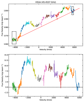
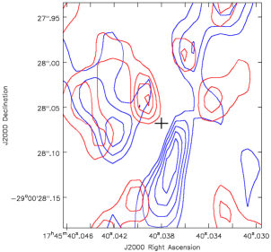
Figure 3: (a Top Left) A scatter plot of the spectrum of H52$\alpha$ emission without continuum subtraction from the inner 0.077${}^{\prime\prime}\times 0.035^{\prime\prime}$ (PA$\sim-2^{\circ}$) of Sgr A* using twelve adjacent spectral windows. (b Botton Left) Continuum subtracted H52$\alpha$ emission from Sgr A* presented in histogram format. This continuum was fit in the range $-4000$ to $-3600$ and $6000$ to $6300$ km s^-1. The spectrum of individual spectral window is scaled such that adjacent spws are continuous. This scaling removes the flux scale across the band which varies at a level of few tenths of a percent. (c Left) Contour levels of red- and blue-shifted components of H52$\alpha$ are set at 0.18, 0.36, 0.54, 0.72 Jy  beam^-1  km s^-1. The beam sizes for the blue- and red-shifted moment maps are $0.075^{\prime\prime}\times 0.034^{\prime\prime}$ and $0.077^{\prime\prime}\times 0.035^{\prime\prime}$, respectively. The blue and red-shifted velocity ranges, in red, blue colors, correspond to $\sim 4000$ and $-2000$ km s^-1, respectively. The drawn cross coincides with the position of Sgr A*.

Before a continuum was fitted and subtracted, it was necessary to manually equalize the flux of each spectral window due to errors in flux calibration. We employed the following procedure beginning with the lowest frequency spectral window $j$: (1) determine the ratio of the mean flux of the last ten channels of spectral window $j$ with the mean flux of the first ten channels of the next (higher frequency) spectral window $j+1$, (2) multiply each channel of spectral window $j+1$ by this ratio to equalize it, (3) repeat the previous steps but now starting with the newly equalized spectral window $j+1$. The derived ratios used to normalize the spws ranged from $0.9832$ to $1.003$. The spectral windows were then concatenated as shown in Figure 3a.

A linear continuum was fit to the concatenated data with channels with no strong line emission chosen between –4200 to –3900 km s^-1and 5800 km s^-1 to 6000 km s^-1. The resultant subtracted spectra is shown in Figure 3b. Note that although the absolute continuum flux is lost in Figure 3a, the line emission flux density is recovered in Figure 3b.

2.1.4 H56$\alpha$ VLA Data

We carried out A-array observations (19A-229) in the (9mm) band on 2019, July 26. We used the 3-bit system and a calibration strategy similar to that employed for the VLA H52$\alpha$ data. Phase self-calibration was applied three times to all the data using the bright radio source Sgr A*. The broad 8 GHz bandwidth is comprised of 64 spws, each having 64 channels of 2 MHz width. We imaged ten individual spws close to the rest frequency of H56$\alpha$ at 36.466 GHz before continuum subtraction. These spectral windows correspond to a velocity range between $\sim$–4000 km s^-1 and +6300 km s^-1.

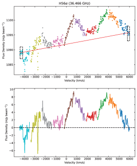
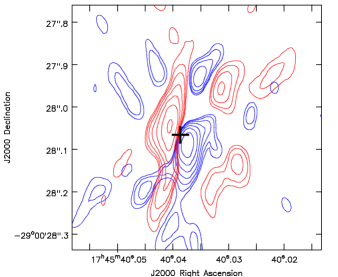
Figure 4: (a Top Left) A scatter plot of the spectrum of H56$\alpha$ emission without continuum subtraction from the inner 0.22${}^{\prime\prime}\times 0.27^{\prime\prime}$ of Sgr A* using ten adjacent spectral windows. The rest frequency of H56$\alpha$ transition is at 0 km s^-1. (b Bottom Left) Continuum subtracted H56$\alpha$ emission from Sgr A* presented in histogram format. The spectrum of individual spectral window is scaled such that adjacent spws are continuous. This scaling removes the flux scale across the band which varies at a level of few tenths of a percent. (c Right) Contour levels of red- and blue-shifted components of H56$\alpha$ are set at 1, 1.5, 2.25, 3.38, 5.06, 7.6 and 11.4 mJy per $0.099^{\prime\prime}\times 0.05^{\prime\prime}$ beam and $0.095^{\prime\prime}\times 0.049^{\prime\prime}$ beam, respectively. The blue and red-shifted velocity ranges, in red, blue colors, correspond to $\sim 4000$ and $-2000$ km s^-1, respectively. The drawn cross coincides with the position of Sgr A*.

Continuum subtraction was performed with the same technique that was applied to the H52$\alpha$ line data. A linear continuum was fit to the concatenated data with channels chosen between –4400 to –4150 km s^-1and 5800 km s^-1 to 6000 km s^-1. The resultant with and without continuum subtracted spectra are shown in Figure 4a,b, respectively.

2.2 Spectroscopic Results

To confirm the results presented by Murchikova et al. (2019), we used the four independent measurements of H30$\alpha$, H39$\alpha$, H52$\alpha$ and H56$\alpha$ with different spectral setups. Despite having significantly broader spectral coverage than Murchikova et al. (2019), it is still not clear where the true continuum is because of a limited set of line free channels. Clearly, a different spectral setup is required in the future to determine true line free channels for proper continuum subtraction.

2.2.1 H30$\alpha$ Line Emission

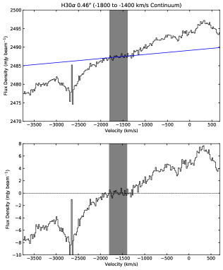
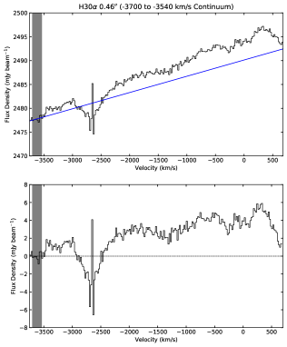
Figure 1: (a Top Left) The spectrum of Sgr A* integrated over a beam with a diameter of 0.46^′′ is shown before continuum subtraction. In order to confirm the double-peak spectrum of Sgr A*, we used similar parameters to those of Murchikova et al. (2019), assuming line free channels at velocities between –1300 and –1800 km s^-1  (the shaded region). The overlayed line is the least squares straight-line fit to the continuum in the shaded region. (b Bottom Left) Identical to (a) except that the continuum has now been subtracted from the spectrum. The vertical gray bars show the selected line free channels. (Top Right c, Bottom Right d) As for Figure 1 except line free channels are instead chosen from –3600 and –3800 km s^-1  (the shaded region). As before the top panel is before continuum subtraction and the bottom panel is post continuum subtraction.

We extracted H$30\alpha$ spectrum using the same scale size and spectral resolution that were used by Murchikova et al. (2019). However, our spectral coverage is wider than that shown by Murchikova et al. (2019). As a result, we selected two different sets of line free channels. The first was chosen to confirm the double-peak spectrum of Sgr A* as seen by Murchikova et al. (2019). Channels between velocities of –1300 km s^-1 and –1800 km s^-1 were used in a linear $\chi$-squared fit in the image plane to subtract the continuum. This mimics a line free channel selection process if bandwidth was not available beyond –1800 km s^-1. Figure 1a,b shows the spectra of Sgr A* before and after the continuum subtraction, respectively. The subtracted linear fit in Figure 1b shows a spectrum with similar shape to that presented by Murchikova et al. (2019). This confirms the double-peak spectrum of Sgr A* at $\sim\pm$500 km s^-1  utilizing a different technique in continuum subtraction. The only significant difference to Murchikova et al. (2019) is a higher estimated flux density by $\sim$10 mJy. This is likely the result of the amplitude and phase self-calibration applied to our data. Atmospheric phase errors can cause reduced flux densities of Sgr A* if proper self-calibration is not carried out. Alternatively, it is possible that the stimulated emission from ionized gas toward Sgr A* is time variable and is responsible for different flux density measured at different epochs.

The second set of line free channels was selected at the extreme end of blue-shifted velocities between –3600 and –3800 km s^-1. Figure 1c,d shows the constructed spectra before and after applying continuum subtraction, respectively. There is a broad absorption line centered at –2600 km s^-1. Although this absorption contaminates the emission from Sgr A*, it nevertheless shows emission that extends beyond –1500 km s^-1. The data presented by Murchikova et al. (2019) did not contain velocity coverage beyond –2000 km s^-1. Thus, we tentatively show evidence of highly blue-shifted velocities extending to –3500 km s^-1  and a third high-velocity peak near –2000 km s^-1, in addition to $\pm 500$ km s^-1  peaks.

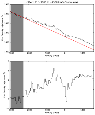
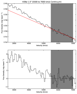
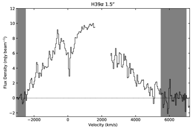
Figure 2: (a Left) Emission with or without continuum subtraction from the inner 0.75^′′ at the peak position of Sgr A* from –3050 km s^-1 to1600km s^-1. A fitted continuum is shown as a result of fitting chosen line free channels from –3000km s^-1 to –2500km s^-1. (b Right) Similar to a except the emission from 2575 km s^-1 to 7200 km s^-1 is shown. The line free channels were chosen as 5500 km s^-1 to 7000 km s^-1 and the resultant fit is drawn. (c Bottom) Excess H39$\alpha$ emission found from subtracting continuum in the respective top panels in (a,b).

Potential sources of the molecular absorption line found at roughly –2665 km/s, as noted in Figures 1 and 2, are identified in the H30$\alpha$ rest frame. The absorption is centered at 233.963 GHz. There are three candidates that could be responsible for the absorption. One is CH₃OH(5(1,5)-4(1,4)) at center frequency 234.01158 GHz which would result in a red-shifted velocity of 62.19 km s^-1. This component has similar velocity to that of dense gas associated with the molecular ring orbiting Sgr A* (e.g., Yusef-Zadeh et al. (2017)), thus this red-shifted gas cloud close to Sgr A* may be detected in absorption against Sgr A*. The others are OS¹⁸O(24(2,22)-24(1,23)) at 233.94997 GHz, blue-shifted by –16.75 km s^-1  or OS¹⁸O(52(7,46)-51(8,43)) centered at 233.9506176 GHz, blueshifted by –15.94 km/s.

2.2.2 H39$\alpha$ Line Emission

Two spectra were obtained over the inner 0.75^′′ towards the position of Sgr A*. With respect to the rest frequency of H39$\alpha$ at 106.737 GHz, one spectral window was available between –3050 km s^-1 to 1600 km s^-1 and the other ranged from 2575 km s^-1 to 7200 km s^-1, as shown in Figure 2. There is no data available between these two spectral windows because of the initial observing setup. A linear continuum was fit individually to each spectra. For the more blue-shifted window, the range –3000 km s^-1 to –2300 km s^-1 was selected, while 5500 km s^-1 to 7000 km s^-1 was chosen for the red-shifted component. The resultant H39$\alpha$ emission with and without continuum subtraction is shown in Figure 2a,b. We note broad H39$\alpha$ line emission from Sgr A*. The emission confirms the results of Murchikova et al. (2019) in that there are two high velocity ionized components peaking at $\sim\pm 500$ km s^-1. Figure 2c also shows excess emission detected at $\sim-2000$ km s^-1, confirming the reality of the H30$\alpha$ peak line emission shown in Figure 1c,d with the caveat that the true line free channels in H39$\alpha$ and H30$\alpha$ are unknown. Thus, we note tentative detection of H$39\alpha$ line emission extending to 5500 km s^-1  reflecting broader velocity coverage towards positive velocities.

2.2.3 H52$\alpha$ Line Emission

We used twelve adjacent spectral windows covering radial velocities between $\sim-4000$ to $\sim 6300$ km s^-1  with respect to the rest frequency of H52$\alpha$ at 45.4538 GHz. The spectra shown in Figure 3a,b were obtained over the inner 0.20${}^{\prime\prime}\times 0.11^{\prime\prime}$ of Sgr A* with a spatial resolution of 77 $\times$ 35 mas and PA$\sim-2^{\circ}$. We detect an excess flux of H52$\alpha$ line emission at roughly $\sim 500$ km s^-1 with a dip near 0 km s^-1  consistent with the earlier H$30\alpha$ measurements (Murchikova et al., 2019). The $-500$ km s^-1  feature is much weaker than the $500$ km s^-1  feature but extends to more negative velocities. In addition, we note enhanced line emission that extends to –1500 and +4000 km s^-1; similar trends are also noted in the H39$\alpha$ spectrum, as shown in Figure 3c.

In order to determine where high velocity ionized features are located with respect to Sgr A*, we selected the spectral windows that showed enhanced –2500 and 4000 km s^-1 peak emission. Using two spectral windows, we made moment maps of five channels centered near the low and high velocity channels (channels 5-10 and 50-55), determined the slope between the low and high velocity features for each spectral window before subtracting them from each other. The resulting continuum subtracted image of Figure 3c shows contours of blue- and red-shifted H56$\alpha$ line emission corresponding to $\sim$–2500 and $\sim$4000 km s^-1, respectively. These high velocity features show a diagonal NE-SW distribution along the Galactic plane similar to that found by Murchikova et al. (2019) at $\pm 500$ km s^-1.

2.2.4 H56$\alpha$ Line Emission

We used ten adjacent spectral windows covering radial velocities between $\sim-4000$ to $\sim+6000$ km s^-1  with respect to the rest frequency of H56$\alpha$ at 36.466 GHz. The spectra shown in Figure 4a,b were obtained over a 0.22${}^{\prime\prime}\times 0.27^{\prime\prime}$ region centered on Sgr A* with a spatial resolution of $\sim 95\times 49$ mas and PA$\sim 82^{\circ}$. We detect an excess flux of H56$\alpha$ line emission at roughly $\sim 500$ km s^-1 with a dip near 0 km s^-1  consistent with earlier H$30\alpha$ measurements (Murchikova et al., 2019). However, the red-shifted component at radio is much stronger than the blue-shifted component which is faint. It is likely that the $-500$ km s^-1  feature that Murchikova et al. (2019) detects at higher frequencies is faint at H56$\alpha$ line but extended to more negative velocities corresponding to $\sim$–2500 and $\sim$4000 km s^-1. These high velocity features show a diagonal NE-SW distribution along the Galactic plane similar to that found by The trend is similar to mm spectra except that enhanced radio recombination line emission at red-shifted velocities are 3-4 times stronger than the emission at blue-sifted velocities. In addition, we note enhanced line emission that extends to –1500 and +4000 km s^-1; similar trends are also noted in the H39$\alpha$ spectrum, as shown in Figure 2c. We note two narrow and one broad absorption feature at velocities between –2500 and –4200 km s^-1. The two narrow absorption lines are detected at 36.796 and 36.947 GHz, and are shown in Figure 4b. The 36.947 absorption line is centered on a broad absorption ranging over a few hundred km s^-1. It is not clear what these lines are. There is a family of methyl cyanide lines that range from 36.7937 - 36.7975 GHz as well as a methanol line at 36.7955 GHz. The latter corresponds to a radial velocity of $\sim-4$ km s^-1with respect to the rest frequency. We also note that acetone lines between 36.952 and 36.940 GHz correspond to 40 km/s and $-$57 km s^-1, respectively. These radial velocities are in the range of velocities detected toward the molecular ring orbiting Sgr A*.

In order to determine where the high velocity ionized features are located with respect to Sgr A*, we selected spectral windows that showed enhanced –2500 and 4000 km s^-1 peak emission. From these windows five channels were averaged near both the low and high velocity band edges (channels 5-10 and 50-55), before subtracting them from each other. The resulting continuum subtracted image of Figure 4c shows contours of blue- and red-shifted H56$\alpha$ line emission corresponding to $\sim$–2500 and $\sim$4000 km s^-1, respectively. These high velocity features show a similar distribution to that found for H52$\alpha$ line emission, i.e., diagonal NE-SW orientation.

3 Continuum Data Analysis and Results

3.1 Data Preparation

We carried out radio continuum observations of Sgr A* at multiple frequencies, each of which is described below. All our continuum observations are centered at the J2000 absolute position of Sgr A*, $\alpha,\delta=17^{h}45^{m}40^{s}.038,-29^{\circ}00^{\prime}28^{\prime\prime}.069$. We used 3C286 to calibrate the flux density scale, 3C286 and J1733-1304 (aka NRAO530) to calibrate the bandpass and J1744-3116 to calibrate the complex gains in all of our observations.

3.1.1 Broadband Q-band (40–48 GHz) and Ka-band (32–40 GHz)

We observed Sgr A* on 2014 February 21 (14A-231) and 2018 April 3 (18A-091) in the most extended A-array configuration at 44 GHz. The Q-band (7mm band) was used in the 3-bit system, which provided full polarization correlations in 4 basebands, each 2 GHz wide, centered around 44.5 GHz. Each baseband was composed of 16 subbands (spws), each 128 MHz wide. Each subband in turn was made up of 64 channels, each 2 MHz wide. This epoch of 44 GHz observation, had effective bandwidth of 8 GHz.

In addition, A-array observations (14A-231, 16B138) in the Ka (9mm) band on 2014, March 9 and 2016 July 19 at 34.5 GHz were carried out. We used the same 3-bit system and the same calibration strategy for Ka band as we did for the Q-band observations. A phase and amplitude self-calibration procedure was applied to all data using Sgr A*. To construct spectra at Ka and Q bands, as shown in Figures 3 and 4, only phase calibration was applied to the VLA data sets.

3.1.2 Broadband Ku band 13–15 GHz

A-array observations (14A-231) were carried out on March 10, 2014 at 14 GHz utilizing full polarization correlations in 2 basebands, each 1 GHz wide between 13.18 and 14.95 GHz. Each baseband was composed of eight 128 MHz wide subbands. Each subband was made up of sixty-four 2 MHz channels for a total effective bandwidth of 2 GHz. All of the subbands were self-calibrated in phase separately. We then combined all 14 useful spectral windows with the task VBGLU in AIPS before we applied additional phase self-calibration.

3.1.3 Broadband X band 8–10 GHz

A-array observations were carried out in two epochs on April 17, 2014, and August 17, 2019 at 8 GHz with identical system setup. We used the same backend as that of Ku data for both data sets but with center frequency at 9 GHz and total bandwidth of 2 GHz. Calibration on both data sets was done independently similar to that of Ku data by phase and amplitude calibration of individual spectral windows. We combined both data sets followed by phase and amplitude self-calibration. All Stokes parameters were calibrated in both data sets.

3.1.4 Broadband L Band 1.4–2 GHz

We carried out broad band VLA A-array observations of the Galactic center at 1-2 GHz on 2014 April 02 (project 14A-231). The system we used provided full polarization in both basebands. Each 1.4 GHz subband was made up of 64 channels of 1 MHz each. Several phase and amplitude self-calibration procedures were applied to the data in OBIT (Cotton, 2008) using the bright radio source Sgr A* before MFImager was used to construct a cube of 16 channels corresponding to each spectral window.

3.2 Radio Continuum Results

We begin first by describing high frequency features within 5${}^{\prime\prime}-10^{\prime\prime}$ of Sgr A* followed by the arcminute structures in the vicinity of Sgr A*. We then argue for a radio jet emanating from Sgr A*. A trace of this jet is revealed at high frequencies, though with low signal-to-noise ratio. Many high frequency features that are described in the vicinity of Sgr A* are several thousand times fainter than the bright source Sgr A*, thus errors generated by the variable, strong continuum from Sgr A* contaminate structural details in its vicinity. To mitigate these difficulties, we focus on persistent structures revealed from multiple observations with different frequencies and baselines.

3.2.1 High Frequency Radio Data

(a) NE-SW features

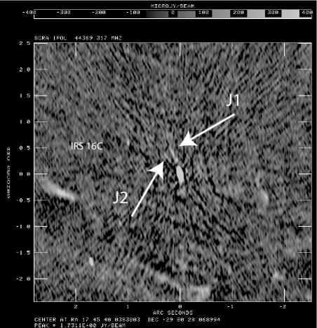
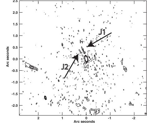
Figure 5: (a) Grayscale continuum image of the inner 2.5^′′ of Sgr A* at 44 GHz with a resolution of $0.087^{\prime\prime}\times 0.036^{\prime\prime}$ (PA=13.41^∘). The dynamic range of this image with the peak flux 1.73 Jy beam^-1 is 3700. (b) The same as (a) except that contours are displayed at levels -100, 100, 200, 300, 400, 500, 1000, 5000, 10000 $\mu$Jy beam^-1. This data set was taken with the VLA on September 16, 2015.

Figure 5 shows a linear feature J1 with a PA$\sim 23^{\circ}$ extending NE of Sgr A* for $\sim 0.4^{\prime\prime}$, and having a typical surface brightness of $\sim 300\,\mu$Jy beam^-1 at 44 GHz. As described below, this feature may be related to a more extended loop-like structure. The rms noise of J1 in the immediate vicinity of Sgr A* is $\sim 46\,\mu$Jy beam^-1. There is also a fainter feature, J2, which is 1/2 of typical surface brightness of J1, with PA$\sim 39^{\circ}$. The latter needs to be confirmed, though it is likely to be associated with large-scale features J5, as described below. The PAs of J1 and J5 range between 23^∘ and 59^∘ and are similar to the PAs of highly red-shifted RRL components, as shown in Figures 3 and 4, and mmRL reported by Murchikova et al. (2019). The H39$\alpha$ and H56$\alpha$ spectra shown in Figures 2 and 4 include the region that contains both J1 and J2. Thus, it is possible that the high velocity redshifted components are related to elongated structures J3 and J5 near Sgr A*, as seen in Figure 5.

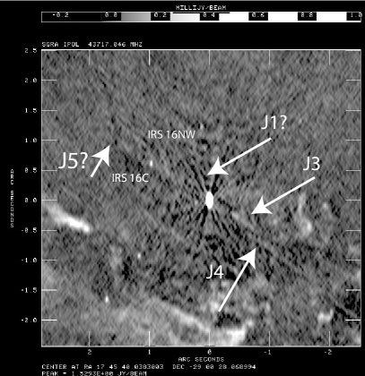
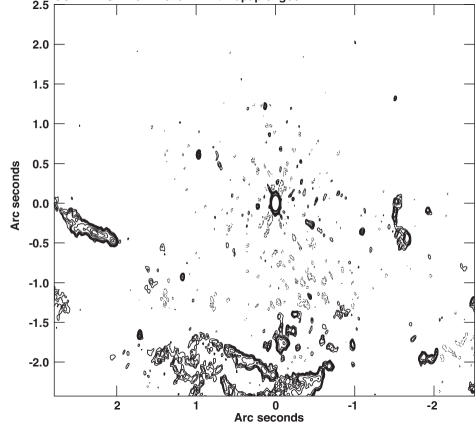
Figure 6: (a) A grayscale image of the inner 2.5^′′ of Sgr A* at 44 GHz with a spatial resolution of $0.075^{\prime\prime}\times 0.037^{\prime\prime}$ (PA=$-0.86^{\circ}$) taken on April 3, 2018. The rms noise is 18$\mu$Jy. Prominent features to the south are associated with the mini-spiral or Sgr A West. (b) The same as (a) except that contours are displayed at levels -100, -75, 75, 100, 125, 150, 200, 300, 400, 500, 750, 1000, 5000, 20000 $\mu$Jy beam^-1.

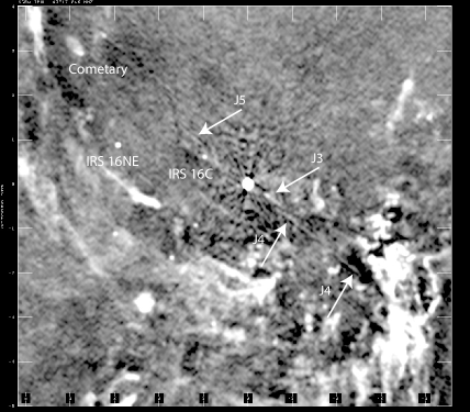
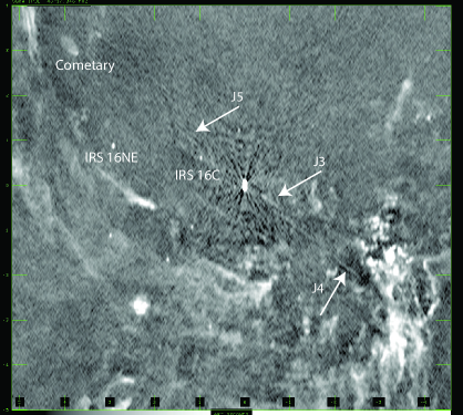
Figure 7: (a, b) Two grayscale images of the inner 4^′′ of Sgr A* at 44 GHz with two different brightness contrasts. The images are similar to Figure 6 except they are convolved with a 0.076^′′ Gaussian beam. The rms noise is 21$\mu$Jy. The prominent feature to the west is the mini-cavity.

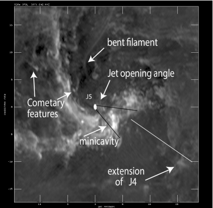
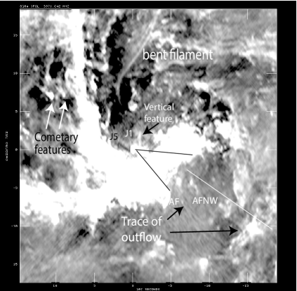
Figure 9: (a, b) Grayscale 9 GHz continuum images of the inner of 20^′′ of Sgr A* with a resolution of $0.35^{\prime\prime}\times 0.18^{\prime\prime}$ (PA=5.61^∘). The flux density ranges between -0.6 and 10 mJy beam^-1 with two different contrasts. This data set was taken on August 17, 2019. Black lines show the opening angle of the jet arsing from Sgr A* to the SW. The white lines point to a number of sources that lie diagonally along the direction of the outflow.

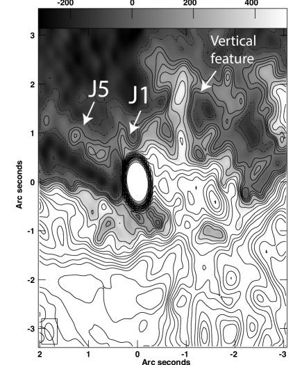
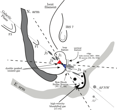
Figure 9: (c) Grayscale contours of 9 GHz emission with levels (-2, -1, 1, 2, 3, 4, 6, 8, 10, 14, 18, 22, 30, 40, 50, 80, 100, 200, 500) $\times 50\mu$Jy beam^-1. (d) A schematic diagram of prominent features in the inner 20^′′ of Sgr A*. The double-peaked blue and red-shifted mmRL emission associated with Sgr A* is shown in color. The positions of some of the sources, such as bow-shock sources, indicated on this figure may not be accurate.

Figure 6 shows another 44 GHz image of the same region based on our second epoch observation. This image has a dynamic range of $\sim 9000$ and rms noise of 17 $\mu$Jy beam^-1. We note a weak elongated feature J5 with a surface brightness of $\sim 50\mu$Jy beam^-1 to the NE of IRS 16C and a PA$\sim 59^{\circ}$. Two faint linear features J3 and J4 are also found to the SW of Sgr A* with surface brightness of 20-100 $\mu$Jy beam^-1. The position angles of J3 and J4 are 51^∘ and 57^∘, respectively. In order to enhance the signal-to-noise ratio of J3, J4 and J5, Figures 7a,b present the inner 5^′′ of Sgr A* with a convolved resolution of 76 milliarcsecond (mas). All three features have PAs within six degrees of each other. The longest linear feature is J4 with an extent of $\sim 3.^{\prime\prime}5$. A 9 GHz image of this region in Figure 9d with lower spatial resolution than Figure 7 shows the same elongated structure emanating from Sgr A*. The PAs of these features appear to be in the direction where IRS 16C as well as cometary radio and near-IR stellar sources (F1, F2, F3, X3, X7, X8) lie (Muzić et al., 2007, 2010; Yusef-Zadeh et al., 2016; Peißker et al., 2019).

We notice that in numerous high frequency, high resolution images, the rms noise increases only within $\sim 1^{\prime\prime}$ of Sgr A*. For example, the rms noise in Figure 6 is about three times higher. It is possible that phase and amplitude errors are responsible for the increased noise. Alternatively, the excess noise is due to diffuse emission at 44 GHz and is intrinsic due to residual synchrotron emission detected at mm and X-rays. This is a region where diffuse mm and X-ray emission has previously been detected (Wang et al., 2013; Yusef-Zadeh et al., 2017). Thus, that the dynamic range may be limited due to highly turbulent multi-phase medium.

(b) western minicavity

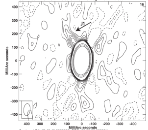
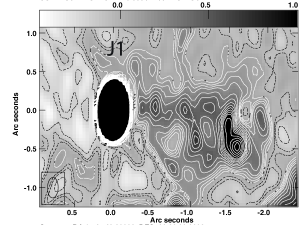
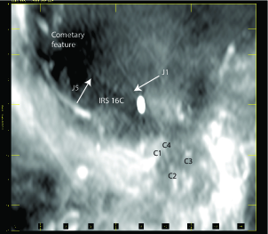
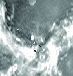
Figure 8: (a) Top Left Contours of 35.72 GHz emission from the inner 0.45^′′ of Sgr A* observed on March 9, 2014 at levels of (-2, -1, 1, 2,…, 8, 10, 50, 100, 200) $\times 81\mu$Jy beam^-1. The 8-GHz bandwidth was imaged in 24 different frequency channels and this map corresponds to channel 16. The resolution of the image is $0.090^{\prime\prime}\times 0.049^{\prime\prime}$ (PA=-5.38^∘). (b) Top Right Greyscale contours of 8.9 GHz emission with levels at (-2, -1, 0..5, 0.5, 1, 1.5, 2, 3,…, 10, 12, 14,….20) $\ times$ 0.1 mJy beam^-1. of $0.26^{\prime\prime}\times 0.14^{\prime\prime}$ (PA=$-1.5^{\circ}$). (c) Bottom Left A grayscale 15 GHz image of the inner 4^′′ of Sgr A* with a resolution of $0.22^{\prime\prime}\times 0.11^{\prime\prime}$ (PA=5.25^∘). The highly blue-shifted negative velocity features are labeled C1 to C4 (Royster et al., 2019). (d) Bottom Right A 9 GHz image from data, as in (c), shows a grayscale image of the inner 4^′′ of Sgr A*.

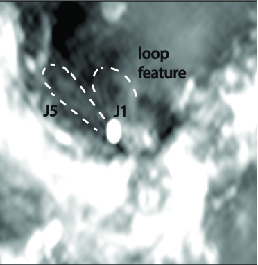
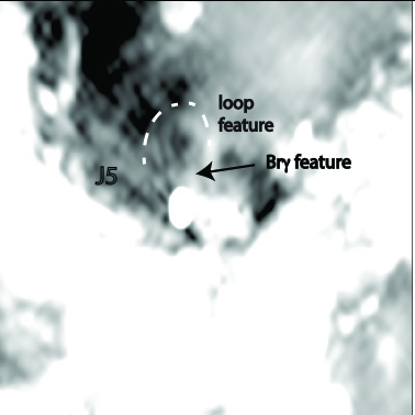
Figure 8: (e) Top A greyscale image of 9 GHz image using data taken in 17 April, 20014 with a resolution of $0.36^{\prime\prime}\times 0.22^{\prime\prime}$ (PA=-1.88^∘). We used OBIT by splitting the 2 GHz bandwidth of 9 GHz data into 46 channels to account for frequency response of Sgr A* in each frequency channel before the final image was made. Similar imaging was done with data taken on 17 August, 2019 and the features described here were identified in both epochs. (f) Bottom Similar to (e) except with different contrasts to bring out faint features.

Figure 8a shows a 36.8 GHz contour image of the inner 0.4^′′ of Sgr A* constructed from data taken on 2016 July 19. The linear feature J1 is detected at a PA$\sim 26^{\circ}$. Figure 8b shows contour emission from the inner 1^′′ of Sgr A* with a view of J1 based on a 9 GHz observation carried out on 2014 April 17. Again we notice an extension of J1 with similar PA to that at 36.8 GHz. Figure 8c shows the inner 4.5^′′ of Sgr A* at 15 GHz where we note two faint linear features directed to the NE of Sgr A*. Both features, though with low signal-to-noise ratio, appear to have a coherent structure with similar PAs to J1 and J5, detected at other frequencies. Figure 8d shows a greyscale image of the inner 4^′′ of Sgr A* at 9 GHz. The region to the southwest of Sgr A* in Figure 8c,d contains highly blue-shifted ionized gas associated with the minicavity and a string of highly blue-shifted compact velocity features which appear to bridge Sgr A* to the western edge of the mini-cavity. Compact sources, labeled C1 to C4, are identified to have extremely blueshifted ionized gas within 0.2pc of Sgr A* from –480 to –300 km s^-1 (Royster et al., 2019). The highly blue-shifted ionized gas has been detected not only toward C1-C4, as labeled on Figure 8c,d, but also toward the minicavity (Zhao et al. (2010) and multiple compact sources that lie close to the western edge of the minicavity. Figure 8d shows a linear feature J4, as shown in Figure 6a, that appears to cross a string of HII regions, including C3. An excess of FeII/III line emission (Lutz et al. 1993) and disturbed kinematics from the western edge of the mini-cavity are unlikely to be due to orbital motion because enhanced FeII/III line emission is detected only in the mini-cavity. An external source of outflow impacting the orbiting gas is likely to be responsible for producing shocked gas, shaping morphological, kinematic structures to the SW of Sgr A* (Yusef-Zadeh et al., 2016; Royster et al., 2019). Lastly, Figures 8e,f show detailed images of the inner 4^′′ constructed by combining two epochs of 9 GHz data. We note that J2 and J5 appear to be parts of a coherent elongated 4^′′ structure that extends the NE of Sgr A*. A loop-like feature is also noted extending from the vertical feature to the NE of Sgr A*. It is possible that J1 is part of this loop feature within which there are additional diffuse features. A north-south feature appears to be the radio counterpart to a Br$\gamma$ ionized bar that has recently been studied (Peißker, et al., 2020). Figure 9c also shows contour representation of the Br$\gamma$ feature lying between J1 and the vertical feature.

(c) EW ridge

Figure 8 shows an EW ridge of mm emission which extends to the west of Sgr A* for $\sim 2^{\prime\prime}$. This is also prominently detected at 224 GHz within which a number of radio sources, RS1-RS8, and a cluster of dusty infrared sources lie (Yusef-Zadeh et al., 2017; Peißker et al., 2020). The trajectories of dusty stellar sources detected at infrared indicate that they are in an elliptical orbital motion around Sgr A* (Peißker et al., 2020). Unlike many NE-SW features running along the Galactic plane, as described earlier, the EW ridge has a different orientation detected only on the western side of Sgr A* but nevertheless appears to be associated with Sgr A*. The EW ridge is revealed best at high radio frequencies, millimeter and infrared, suggesting that it consists of a mixture of dust, gas and dusty stellar sources. The kinematics of dusty stellar sources in the ridge indicate that they are in an elliptical counter-rotating orbit around Sgr A* (Peißker et al., 2020), suggesting that they are impacted by a collimated outflow from Sgr A*, as argued below.

To examine the morphology of the mini-cavity further, Figures 9a,b present 9 GHz images of the inner 20^′′ of Sgr A* with two different brightness contrasts to highlight the bright region of the mini-cavity. The mean flux density in the western edge of the minicavity is twice that of the eastern edge. Assuming that the enhanced emission and the disturbed kinematics are due to a collimated outflow from Sgr A*, the opening angle of the outflow must be $\sim 30^{\circ}$, as indicated in Figure 9a, which covers not only the western half of the mini-cavity but also the EW ridge.

(d) AF and AFNW stars

The SW extension of the minicavity directed towards the southern arm of the minicavity shows a number of elongated sources and a tail of ionized gas crossing the southern arm. Two mass-losing stars AF and AFNW have previously been identified to have cometary tails directed away from Sgr A* (Yusef-Zadeh et al., 2017). These features are likely to reflect the interaction of an outflow from the direction of Sgr A* with stellar sources and orbiting gas. Both the AF and AFNW sources are located within the opening angle of the jet beyond the minicavity; the white lines drawn on Figures 9a,b run parallel to a number of features that trace the direction of the outflow from Sgr A*. lie within the opening angle of the jet. In this picture, infrared stellar sources in the EW ridge are also impacted by this outflow.

(e) bent filament

We also note in Figure 9 a bent filament to the north of Sgr A* (Yusef-Zadeh et al., 2017; Morris et al., 2017). Previous measurements have not been able to determine if this filament is connected to Sgr A* and perhaps produced by Sgr A* (Yusef-Zadeh et al., 2017; Morris et al., 2017). There is no evidence for morphological association with Sgr A* at 9 GHz. We note a compact source with a flux density of 0.15$\pm 0.5$ mJy beam^-1 coinciding with the southern tip of the filament at $\alpha,\delta_{J2000}=17^{h}\,45^{m}\,40^{s}.101\pm 0.002\,-29^{\circ}\,00^{\prime}\,23^{{}^{\prime\prime}}.269\pm 0.118$. To the NE of Sgr A*, J5 and J1 are revealed with an average flux density of $\sim 100$ $\mu$Jy beam^-1 and a PA$\sim 56^{\circ}$ and 21^∘, respectively. The extension of J5 appears to encounter the cometary tail of stellar source F1 to within one degree.

(f) vertical feature

We also note a vertical feature to the NW of Sgr A*. A close up of this region, shown in Figure 9c, indicates a continuous structure from the eastern boundary of the minicavity. There is no kinematic information but it appears that the ionized gas associated with the eastern boundary of the minicavity is turning counterclockwise as it orbits Sgr A*. A schematic diagram of features noted at high frequencies is shown in Figure 9d.

3.2.2 Low Frequency Radio Data

(a) NE-SW radio jet

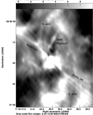
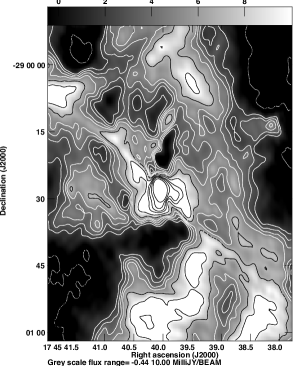
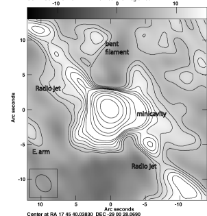
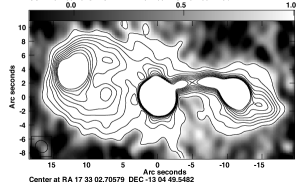
Figure 10: (a) 1-1.4 GHz image of the mini-spiral constructed by combining eight spectral windows with a resolution of $2.68^{\prime\prime}\times 2.01^{\prime\prime}$ (PA=36^∘). (b) Identical to (a) except grayscale contours are presented with levels -2, 2, 3, 4, 5, 7, 10, 15, 20, 30, 50 mJy beam^-1. The coordinates are shown as offsets from the peak position of Sgr A*. (c) Contours of 20cm emission from a narrow spectral window between 1.25 and 1.31 GHz with levels at (-4, 4, 5, 6, 7, 8, 9, 10, 15, 20 30, 50, 100) $\times$ 2 mJy beam^-1 with a spatial resolution $2.94^{\prime\prime}\times 2.17^{\prime\prime}$ (PA=37.8^∘). (d) Radio emission from the calibrator J1733-1304 corresponding to the lowest frequency spectral window at 1.0 GHz with a peak flux density of 4.02 Jy beam^-1 and contour levels set at (1, 2, 3,….,9)  mJy beam^-1 with a resolution of $1.85^{\prime\prime}\times 1.65^{\prime\prime}$ (PA=49.92^∘).

We have constructed images based on low-frequency data taken with the VLA using its broad band capability. Figure 10a,b show grayscale and contours of 20 cm continuum emission from the inner $\sim 35^{\prime\prime}$ of Sgr A*. These images are constructed by combining spectral windows with frequencies between 1 and 1.4 GHz. A prominent linear structure at PA$\sim 60^{\circ}$ is detected symmetrically only at the lowest frequencies of the broad band. The arms of the mini-spiral are seen in absorption against the strong nonthermal emission from the shell-type Sgr A East SNR, known to lie behind Sgr A* (Yusef-Zadeh et al., 1986; Pedlar et al., 1989). The bent filament with PA$\sim-30^{\circ}$ is seen immediately to the north of Sgr A* (Yusef-Zadeh et al., 2017; Morris et al., 2017).

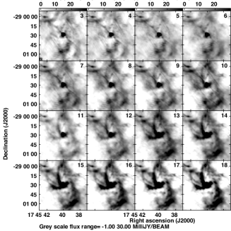
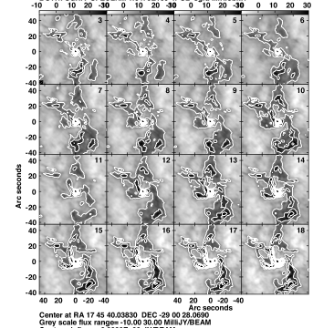
Figure 11: (a) Channel maps corresponding to 16 spectral windows are labeled between 1 and 2 GHz. Black traces radio emission whereas white in the minispiral is seen in absorption. These channel maps reveal both thermal and nonthermal sources simultaneous across the 1 GHz bandwidth in the L band. (b) Channel maps corresponding to 16 spectral windows are labeled between 1 and 2 GHz. Black traces radio emission whereas white is seen in absorption. These channel maps reveal both thermal and nonthermal sources simultaneous across a 1 GHz bandwidth.

In order to show how features projected against a strong nonthermal source, i.e. Sgr A East, are identified, we present grayscale and contour images of all 16 spectral channels between 1 and 2 GHz, as seen in Figure 11a,b. At frequencies $>1.5$ GHz, thermal emission from the mini-spiral is bright and stronger than the background nonthermal emission from the Sgr A East SNR. On the other hand at low frequencies (1-1.4 GHz), the ionized gas of the mini-spiral becomes optically thick and is only detected in absorption against the strong nonthermal background emission. A "sweet spot", 1.4 GHz, demarcates where thermal and nonthermal emission dominate at higher and lower frequencies, respectively.

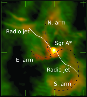
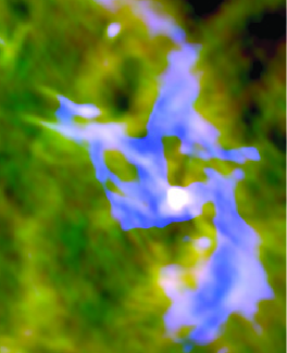
Figure 12: (a) A composite color image of the inner 60${}^{\prime\prime}\times 75^{\prime\prime}$ of Sgr A* between 1-2 GHz. The mini-spiral thermal feature and the nonthermal linear features are labeled. The image is constructed by using a narrow spectral window between $\sim 1.25$ and $\sim 1.31$ GHz and a broad image taken between 1.6 and 1.9 GHz. The mini-spiral thermal feature becomes optically thick (thin) at low (high) frequencies, thus the jet-feature (the mini-spiral) becomes more visible. (b) Another composite color image using three different ranges of emission between 1 and 1.9 GHz. The blue represents the integrated intensity due to eight high frequency spectral windows, while the red represents the eight low frequency spectral windows. The green color represents the entire bandwidth.

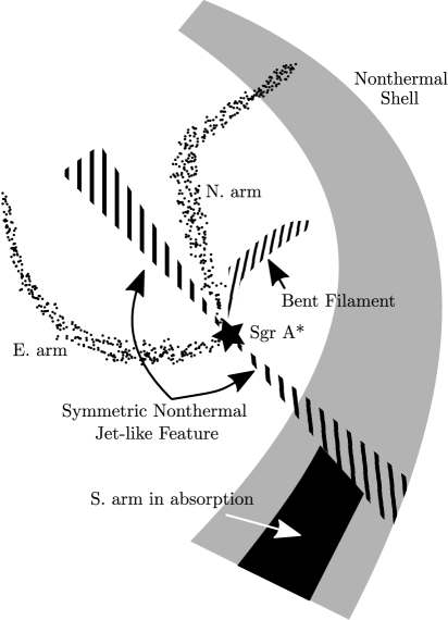
Figure 12: (c) A schematic diagram showing prominent nonthermal (hatched) and thermal (dotted) features at 20cm including a symmetric jet-like feature with respect to Sgr A* and a bent jet-like feature to the north of Sgr A*.

Figure 12a shows a composite image of nonthermal and thermal sources within 30^′′ of Sgr A*. Low frequency (1–1.4 GHz) and high frequency images (1.5–1.9 GHz) are shown in red and blue whereas green shows an image using the entire range (1–1.9 GHz). We note that the optically thick ionized gas associated with the mini-spiral is absent at low frequencies (red) and becomes optically thin at higher frequencies (blue). Figure 12b shows another color image constructed from combining a narrow low-frequency channel map (green) and a broad high frequency channel map (red). The linear nonthermal features are best seen at low frequencies where thermal emission is suppressed. These images confirm that the ionized mini-spiral features are in front of the nonthermal emission. More importantly, new linear features, a radio jet and the bent filament are detected at low frequencies below 1.4 GHz, consistent with being nonthermal. Figure 12c shows a diagram of the prominent thermal and nonthermal components surrounding Sgr A*.

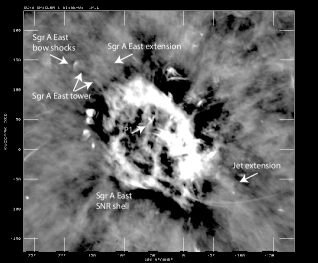
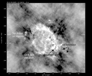
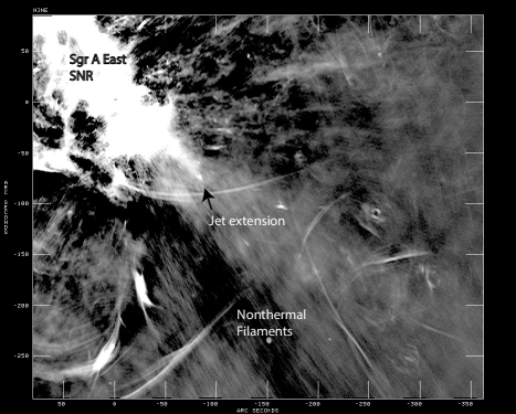
Figure 13: (a Left) Images of the Sgr A East SNR and the mini-spiral are shown using the 20cm broad band between $\sim$1 and $\sim$1.9 GHz with a resolution of $2^{\prime\prime}.68\times 2^{\prime\prime}.03$ (PA=36${}^{\circ}.38$). (b Right) Similar to (a) except a narrow band at 1.24 GHz is displayed. (c Bottom) Broad band 20cm VLA image of the region to the SW of Sgr A* with a resolution of $1.69^{\prime\prime}\times 0.65^{\prime\prime}$ (PA=170${}^{\circ}.56$).

Figure 13a,b show a larger view of the region on a scale of arcminutes where the mini-spiral, the Sgr A East SNR and a string of HII regions at the eastern edge of the Sgr A East shell lie. Unlike the broad band 20 cm image of Figure 13a, the narrow band image of Figure 13b shows the same region where the low frequency radio jet is detected. The position angle of the narrow jet runs $20^{\circ}$ above the Galactic plane at negative longitudes, centered on Sgr A*.

Figure 13c shows a close-up view of the southern extension of the radio jet and a number of Galactic center nonthermal radio filaments. The prominent shell of the Sgr A East SNR is known to be elongated along the Galactic plane. One possibility that could explain the shape of Sgr A East is that the expansion occurred in a medium that had become anisotropic by an earlier outflow driven by the jet activity of Sgr A* along the Galactic plane. In this picture, the oval shape of the shell is produced by the material being swept along the outflow axis to the onset of SNR expansion. The magnetic field along the Galactic plane could also contribute to the formation of the elongated Sgr A East shell.

A 327 MHz image of large scale structures in the Sgr A complex also shows extensions of arcminute jet feature along the Galactic plane. The 327 MHz feature extends up to about 5^′ away from Sgr A* (see Figure 2 of Nord et al. (2004)) having PAs similar to arcminute scale structures revealed at 1.4 GHz. Thus, it is possible that the jet to the NE of Sgr A*, extends to $\sim 10^{\prime}$ (24 pc). High resolution broad band observations are needed to determine the association of linear features detected at 327 MHz with those at 1.4 GHz.

4 Discussion

The Galactic center is a challenging site to search for a jet near Sgr A* because the dynamic range of high resolution images is limited by confusing sources, limited uv coverage, and the intrinsic hourly time variability of Sgr A*, especially at high frequencies. It is also difficult to identify nonthermal sources because at low frequencies (325 MHz), the mini-spiral of ionized gas orbiting Sgr A* is seen in absorption due to optical depth effects. At higher frequencies (8 GHz), thermal features dominate the emission, making it difficult to identify nonthermal sources. One approach to identify both thermal and nonthermal sources is to employ broad bandwidths at multiple frequencies. The upgraded VLA 1-2 GHz band, has changed our view of this region studied by traditional narrow band observations. New images are providing evidence for a linear feature with the appearance of a symmetrical jet originating from Sgr A*, pointing in the direction of the Galactic plane.

4.0.1 Collimated Outflow and Interaction Sites

The overall distribution of the PAs of the linear features described here range between $\sim 30^{\circ}$ and $\sim 60^{\circ}$. As we discuss below, the inferred position angle of the jet is supported by sources within the opening angle of the jet showing kinematical signatures of interactions with an anisotropic outflow. In addition, the inferred jet and outflow properties are consistent with what is expected from models of the interaction of the stellar winds from the WR stars on the central parsec with Sgr A*.

First, the mini-cavity to the SW of Sgr A* shows the highest radial velocities and electron temperatures from radio recombination lines, as well as excess FeII/III and FeIII/Br$\gamma$ line ratios (Lutz et al., 1993; Zhao et al., 2010; Yusef-Zadeh et al., 2012; Peißker et al., 2019, 2020). Radio images presented here clearly indicate an increase in the surface brightness of the western edge of the cavity. There is also the EW ridge showing similar characteristics to the mini-cavity, e.g., excess FeII/III and FeIII/Br$\gamma$ line ratios.

Recent spectroscopic studies suggest dust embedded pre-main sequence stars in the EW ridge (Peißker et al., 2019). All these indicate shock excitation due to violent disturbance. We previously used the implied rate of change in momentum of the disturbed gas and the angle that the western edge of the cavity subtends from Sgr A* to infer that the (two-sided) jet momentum and opening angle are approximately 0.1 $M_{\odot}$ yr^-1 km s^-1 and 30°, respectively. We assume that the jet is mildly relativistic, with $\beta\gamma=3$, implying a rest mass outflow rate $\approx 1\times 10^{-7}$ $M_{\odot}$ yr^-1 (Yusef-Zadeh et al., 2017).

Other observations that can be explained by the impact of the jet with the mini-cavity is an X-ray source with a luminosity of 2$\times 10^{33}$ erg  s^-1 coincides with the cluster of stars, IRS 13E, (Wang et al., 2020; Zhu et al., 2020) embedded within the western edge of the minicavity. Recent analysis of X-ray data concludes that colliding winds of mass-losing stars in the cluster are responsible for production of X-rays (Wang et al., 2020; Zhu et al., 2020). Alternatively, we note that X-ray emission from the minicavity can also be explained by the violent collision with the jet shocking the gas to high temperatures. I another hard X-ray observations between 20-40 keV over the inner few arcminutes of of Sgr A* show extended symmetric emission with respect to Sgr A* along the Galactic plane (Perez et al., 2015). The diffuse hard X-ray emission is interpreted to be due to a population of compact objects or particle outflow from Sgr A*. If the latter, the jet-picture discussed here is likely to explain the origin of diffuse X-ray emission.

Furthermore, gas compression can in principle increase the gas density to overcome tidal shear by Sgr A*, thus inducing star formation activity. Recent measurements Recent spectroscopic studies suggest dust embedded pre-main sequence stars in the EW ridge as as well as bipolar CO outflows indicating young star formation activity near Sgr A*(Yusef-Zadeh et al., 2017; Peißker et al., 2019).

Second, a chain of radio blobs linking Sgr A* and the western edge of the minicavity (Wardle, & Yusef-Zadeh, 1992), show the highest velocity ionized gas, $\sim-300$ to $-480$ km s^-1  detected beyond the inner 1^′′ of Sgr A* (Royster et al., 2019). Along the axis defined by the detection of highly blue-shifted ionized gas, the cometary dusty stellar sources, X3, X7, and X8 are also found to the SW of Sgr A* along the extension of the jet feature (Muzić et al., 2007, 2010; Peißker et al., 2019). These sources show a high abundance of [FeIII] line emission, with similar characteristics to the western edge of the minicavity (Peißker et al., 2019). To the NE of Sgr A*, there is evidence of an elongated X-ray structure, NE plume in Yusef-Zadeh et al. (2012), a number of cometary stellar sources pointing towards Sgr A* (F1, F2, F3) and red-shifted ionized gas (Muzić et al., 2007, 2010; Royster et al., 2019). Muzić et al. (2010) suggested that an external wind with density $\sim 10$ cm^-3 and speed $\mbox{\hbox to0.0pt{\hbox{\lower 5.0pt\hbox{$\sim$}}\hss}\hbox{$>$}}1000$ km s^-1  emerging from the close vicinity of Sgr A* is responsible for shaping the bow shocks and orienting them towards Sgr A*. The inferred ram pressure, $\rho\,v^{2}\sim 2\times 10^{-7}$ dyn cm^-2 is one twentieth of the jet ram pressure thought to be responsible for the formation of the minicavity, As a working hypothesis we assume that the opening angle of the outflow is 60°, with the inner 30°occupied by a mildly relativistic jet. In this picture, the EW ridge at a PA $\sim$30°away from the direction of the relativistic jet is mainly produced by the interaction of the outflow with dusty infrared stellar sources.

Third, on scales of a few mpc, H30$\alpha$, H39$\alpha$ and H56$\alpha$ spectra exhibit broad blue- and red-shifted line emission with a line width of thousands of km s^-1  and oriented roughly along the Galactic plane to the NE and SW, respectively. These have previously been interpreted as the red and blue lobes of a highly inclined Keplerian disk (Murchikova et al., 2019). However, our observations have wider frequency coverage and find significantly broader line widths, $\mbox{\hbox to0.0pt{\hbox{\lower 5.0pt\hbox{$\sim$}}\hss}\hbox{$>$}}4000$km s^-1consistent with Keplerian motion at about 1/5 the observed angular scale of the emission. Instead, this emission more likely arises from entrained material being accelerated outwards by the jet. The mass of accelerated material cannot easily be inferred from the recombination-line fluxes because of the dominant contribution of stimulated emission. The upper limit on the Br$\gamma$ emission within 0.2^′′ of Sgr A* is $\sim 2\,\textrm{Jy\,}$km s^-1(Ciurlo et al., 2020).

The Br$\gamma$ emissivity for T${}_{e}\sim 10^{4}$ K and n${}_{e}\sim 10^{4}\rm cm^{-3}$ is j${}_{\gamma}\sim 2.7\times 10^{-28}$ erg s^-1 cm^-3 sr^-1 (Hummer and Storey, 1987). The Br$\gamma$ luminosity for a source with volume emission measure VEM=$\int n_{e}^{2}\,dV$, yielding a flux S${}_{\gamma}=(\rm j_{\gamma}\,\rm VEM)/d^{2}\sim 0.96(\rm VEM/(10^{58}\,\rm cm^{-3}))$ Jy  km s^-1  where a Galactic center distance d=8 kpc has been adopted. This implies that the volume emission measure of the material is $\mbox{\hbox to0.0pt{\hbox{\lower 5.0pt\hbox{$\sim$}}\hss}\hbox{$<$}}\,2\times 10^{58}$ cm^-3, and that stimulated emission amplifies the H30$\alpha$ line luminosity by at least a factor of 80 (Murchikova et al., 2019). Our radio continuum observations have tentatively detected this material: the weak, extended features J1 and J3 that lie within $0.2^{\prime\prime}$ of Sgr A* have flat spectra between 9 and 44 GHz, consistent with optically-thin thermal bremsstrahlung from the red- and blue-shifted components of this gas, respectively. J3 lies in an area confused by extended continuum emission, making it difficult to extract reliable fluxes, so we focus on J1, which has an integrated flux $\sim 0.2$ mJy at 36 GHz. The free-free emissivity at 36 GHz is j${}_{\nu}/n_{e}^{2}\sim 2.2\times 10^{-40}\,\textrm{erg}\,\textrm{cm}^{3}\,\textrm{Hz}^{-1}\,\textrm{sr}^{-1}$, yielding a flux S${}_{\nu}=\textrm{j}_{\nu}\,\textrm{VEM}/\rm d^{2}\sim 0.32\,\textrm{VEM}/(10^{58}\,\rm\textrm{cm}^{-3})$ mJy. Thus, we infer $\textrm{VEM}\approx 6\times 10^{57}\,\textrm{cm}^{-3}$ for nominal temperature $10^{4}$ K. Adopting dimensions $0\aas@@fstack{\prime\prime}2\times 0\aas@@fstack{\prime\prime}02\times 0\aas@@fstack{\prime\prime}02$ consistent with Fig. 6(b) this implies $n_{e}\approx 1\times 10^{5}\,\textrm{cm}^{-3}$ and mass $\approx 6\times 10^{-5}\hbox{$M_{\odot}$}$.

One of the implications of the presence of ionized gas on such a small scale associated with Sgr A* is that it can also explain the large rotation measure detected toward Sgr A* (RM$\sim-5\times 10^{5}$  rad m^-2) (Bower et al., 2018). Assuming that the parallel component of the magnetic field is 1.5 mG, high velocity ionized gas detected within 0.1^′′ of Sgr A* can produce the observed Faraday rotation.

Fourth, on a scale of AU, the polarization angle of near-IR flaring activity of Sgr A* can be measured several times a day. These measurements give a mean polarization angle of 60${}^{\circ}\pm 20^{\circ}$ consistent with the position angle of the larger scale jet features (Eckart et al., 2006; Meyer, et al., 2007). In addition, VLBI measurements provide highest resolution images of millimeter emission from Sgr A* with mas size scales. The PA of millimeter emission from Sgr A* is roughly in agreement with a PA within 30^∘ of the Galactic plane. Thus, this emission could be associated with the large scale jet feature having similar PA.

Fifth, the linear pc-scale jet-like features that we have identified are stronger at 9 GHz than at 44 GHz, suggestive of synchrotron emission from a jet emerging from the vicinity of Sgr A*. This confirms our earlier narrow band observations reporting a tentative detection of continuous linear structure with an extent of $\sim$3 pc and PA$\sim 60^{\circ}$ (Yusef-Zadeh et al., 2012). The extension of this feature appears to terminate symmetrically by linearly polarized structures at 8.4 GHz, $\sim 75^{\prime\prime}$ from Sgr A* (Yusef-Zadeh et al., 2012). For the observed jet diameter ($\approx 2\arcsec$) and 1.6 GHz surface brightness $\approx 0.2\,\textrm{mJy}\,\textrm{beam}^{-1}$, we deduce an equipartition magnetic field $\sim 0.2$ mG using standard (but uncertain) assumptions: an $E^{-2}$ electron spectrum running between 10 MeV and 100 GeV and equal energy density in electrons and protons.

Finally, the NE edge of Sgr A East is highly distorted along the Galactic place (Yusef-Zadeh et al., 2016). In the jet picture, the kinetic luminosity of the jet is likely responsible for the distortion of Sgr A East. In addition, the puzzle of why the Sgr A East shell is elongated along the Galactic plane can also be explained by a medium that has been swept by a symmetric outflow from Sgr A* along the Galactic plane before the expansion of the remnant occurred.

The six characteristics described above provide overwhelming evidence for a jet extending from AU to pc scales likely surrounded by a wider-angle outflow in the inner parsec.

4.1 Orientation of the Jet

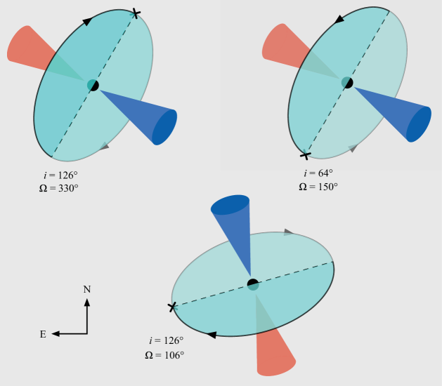
Figure 14: (a,b top Left and Right) Two possible orientations of the accretion disk presumed to be driving the jet from Sgr A*, as viewed by an observer. The red and blue cones represent the red and blue-shifted arms of the jet, which have PA 60 and 240 °E of N, respectively. The jet axis is perpendicular to the plane of the disk (cyan), which may rotate clockwise (left) or counter clockwise (right). The corresponding PA of the ascending node, $\Omega$, is indicated in each case. (c Bottom) For comparison, we show a jet-disk system with orbital plane matching that of the clockwise stellar disk.

The orientation, and mass flow rate of the jet is consistent with jet-launching models, which predict that the jet emerges perpendicular to the equatorial plane of the accretion flow near the event horizon of Sgr A*. Here we define the jet orientation to be the 3D unit vector parallel to the red-shifted component, which we quantify by two angles, $\Omega_{j}$, the PA of the arm (measured E of N), and the angle $\theta_{j}$ that the arm makes to the line of sight (so $0\degr\leq\theta_{j}\leq 90\degr$). The inferred jet is aligned roughly NE-SW on the sky, and given that the disturbed material in the mini-cavity is blue shifted, we infer that the mini-cavity and the ionized bar lie in front of Sgr A* and that the SW arm of the jet is approaching us. Thus the red shifted arm of the jet emerges to the NE of Sgr A* with PA $\Omega_{j}\approx 60\degr$ E of N and makes an angle $\theta_{j}\approx 45\degr$ to the line of sight (which is directed away from the observer). The angular momentum of the inner accretion flow on to Sgr A* should then be parallel or anti parallel to the redshifted arm, implying that the orbital elements of the disk, i.e. PA of the ascending node, $\Omega$, and inclination to the plane of the sky, $i$, are either (i) $\Omega=\Omega_{j}-90\degr\approx 330\degr$, $i=180\degr-\theta_{j}\approx 120\degr$, or (ii) $\Omega=\Omega_{j}+90\degr\approx 150\degr$, $i=\theta_{j}\approx 120\degr$. Figure 14a,b show schematic diagrams of the possible orientations of the jet launched from the accretion disk.

Sgr A* is fed by the combined winds of WR stars in the inner $\sim\,0.1$ pc of the Galaxy (Coker and Melia, 1997; Cuadra et al., 2006, 2008; Ressler et al., 2019). The orbits of most of these stars lie in the “clockwise disk” , with orbital planes distributed around a mean PA of their ascending nodes $\Omega\approx 106\degr$ E of N and mean inclination $i\approx 126\degr$ to the line of sight (Bartko et al., 2009; Gillessen et al., 2009; Yelda et al., 2014; Gillessen et al., 2017). Figure 14c shows the orientation of clockwise stellar disk which is thought to be the source of the accreting material. While the stellar disk orientation is significantly misaligned with the average angular momentum of the inner accretion flow inferred from the jet orientation, simulations show that the material in the inner accretion flow was injected with low orbital angular momentum, i.e. the wind material that is ejected antiparallel to the orbital motion of a small number of dominant WR stars (Calderon et al., 2020; Gravity Collaboration, 2020; Ressler et al., 2019, 2020). The inherent granularity of this process introduces significant variations in the orientation of the low-angular momentum material on $\sim 200$ year time scales as the stars move around their orbits (Ressler et al., 2020). Further, astrometric observations of infrared flares with the GRAVITY instrument on board the VLT suggest a hotspot source orbiting Sgr A* with inclination $i\approx 130\degr$ and $\Omega$ most likely to be either $\approx 130\degr$ – consistent with the clockwise stellar disk, or $\approx 300\degr$ – consistent with our observed jet orientation (Gravity Collaboration, 2020). Finally, we note also that the black hole spin, which reflects the accretion of angular momentum by the hole during its life time is likely to be significantly misaligned with the clockwise disk, reflecting instead the accumulation of material over cosmic time. If the net spin is significant, one might expect the inner accretion flow to be forced into alignment with the equatorial plane of the Kerr space time on scales of a few gravitational radii. We conclude then that the misalignment of the jet and the angular momentum of the clockwise disk is not a significant issue.

5 Summary

We presented multi-wavelength spectroscopic and broad band continuum measurements over a wide range of angular scales toward Sgr A* and its local environment. These measurements indicate a jet driven outflow arising from Sgr A* on mpc to pc scales along the Galactic plane. The opening angle of the outflow is 60°, with the inner 30°occupied by the relativistic jet. Our millimeter recombination line data supported earlier studies that the red and blue-shifted ionized gas detected toward Sgr A* lie along the Galactic plane. We argued that the interaction of the collimated outflow with stellar atmospheres and gas clouds can be responsible for disturbed kinematics of ionized gas, enhanced FeII/III and [FeIII] to Br$\gamma$ line ratios, head-tail cometary stellar sources, X-ray emission from IRS 13 and high Faraday rotation observed toward Sgr A*. Shock heated gas resulting from the interaction has other implications such as compressing the gas to possibly overcome tidal shear, thus inducing star formation. The outflow could also shape the elongation of the Sgr A East SNR and be responsible for high cosmic ray ionization rate inferred from H${}_{3}^{+}$ measurements within the molecular ring and the central molecular zone, e.g, (Goto et al., 2014). Furthermore, our radio continuum data demonstrates that lower frequency emission from Sgr A* at $\nu<1.4$ GHz and its environment have the potential to determine the mass of ionized gas. In the jet picture, a significant amount of the power comes out in the form of the kinetic luminosity carrying off energy and angular momentum. This could explain why Sgr A* appears radiatively under luminous.

6 Data Availability

All the data that we used here are available online and are not proprietary. We have reduced and calibrated these data and are available if requested.

References

- Becker et al. (2011) Becker, P. A., Das, S., & Le, T. 2011, ApJ, 743, 47
- Bartko et al. (2009) Bartko, H., Martins, F., Fritz, T. K., Genzel, R., Levin, Y., Perets, H. B., et al. 2009, ApJ, 697, 1741
- Broderick et al. (2011) Broderick, A. E., Fish, V. L., Doeleman, S. S., Loeb, A. 2011, The Astrophysical Journal 738, 38.
- Bower et al. (2018) Bower, G. C., and 12 colleagues 2018, The Astrophysical Journal 868, 101.
- Brinkerink et al. (2019) Brinkerink, C. D., and 23 colleagues 2019, Astronomy and Astrophysics 621, A119.
- Coker and Melia (1997) Coker, R. F. & Melia, F. 1997, ApJ, 488, L149
- Cotton (2008) Cotton, W. D. 2008, Publications of the Astronomical Society of the Pacific 120, 439.
- Cuadra et al. (2008) Cuadra, J., Nayakshin, S., & Martins, F. 2008, MNRAS, 383, 458
- Cuadra et al. (2006) Cuadra, J., Nayakshin, S., Springel, V., & di Matteo, T. 2006, MNRAS, 366, 358
- Ciurlo et al. (2020) Ciurlo, A., Campbell, R. D., Morris, M. R., Do, T., Ghez, A. M., Hees, A., et al. 2020, Nature, 577, 337
- Calderon et al. (2020) Calderón, D., Cuadra, J., Schartmann, M., Burkert, A., & Russell, C. M. P. 2020, ApJ, 888, L2
- Dexter et al. (2020) Dexter, J., Jiménez-Rosales, A., Ressler, S. M., Tchekhovskoy, A., Bauböck, M., de Zeeuw, P. T., et al. 2020, arXiv:2004.00019
- Eckart et al. (2006) Eckart, A., Schödel, R., Meyer, L., Trippe, S., Ott, T., Genzel, R. 2006. Astronomy and Astrophysics 455, 1.
- Falcke and Markoff (2000) Falcke, H., Markoff, S. 2000. Astronomy and Astrophysics 362, 113.
- Hummer and Storey (1987) Hummer, D. G., Storey, P. J. 1987. Monthly Notices of the Royal Astronomical Society 224, 801.
- Goto et al. (2014) Goto, M., and 6 colleagues 2014, The Astrophysical Journal 786, 96.
- Issaoun et al. (2019) Issaoun, S., and 43 colleagues 2019. The Astrophysical Journal 871, 30.
- Li et al. (2013) Li, Z., Morris, M. R., Baganoff, F. K. 2013. The Astrophysical Journal 779, 154.
- Lu et al. (2011) Lu, R.-S., and 7 colleagues 2011 Astronomy and Astrophysics 525, A76.
- Lu et al. (2009) Lu, J. R., Ghez, A. M., Hornstein, S. D., Morris, M. R., Becklin, E. E., & Matthews, K. 2009, ApJ, 690, 1463
- Lutz et al. (1993) Lutz, D., Krabbe, A., Genzel, R. 1993. The Astrophysical Journal 418, 244.
- Gillessen et al. (2009) Gillessen, S., Eisenhauer, F., Trippe, S., Alexander, T., Genzel, R., Martins, F., et al. 2009, ApJ, 692, 1075
- Gillessen et al. (2017) Gillessen, S., Plewa, P. M., Eisenhauer, F., Sari, R., Waisberg, I., Habibi, M., et al. 2017, ApJ, 837, 30
- Gravity Collaboration (2020) Gravity Collaboration, Bauböck, M., Dexter, J., Abuter, R., Amorim, A., Berger, J. P., et al. 2020, A&A, 635, A143
- Johnson et al. (2018) Johnson, M. D., and 14 colleagues 2018. The Scattering and Intrinsic Structure of Sagittarius A* at Radio Wavelengths. The Astrophysical Journal 865, 104.
- Meyer, et al. (2007) Meyer L., Schödel R., Eckart A., Duschl W. J., Karas V., DovVciak M., 2007, A&A, 473, 707
- Markoff et al. (2007) Markoff, S., Bower, G. C., Falcke, H. 2007. Monthly Notices of the Royal Astronomical Society 379, 1519.
- Morris et al. (2017) Morris, M. R., Zhao, J.-H., Goss, W. M. 2017. ApJ, 850, L23.
- Muno et al. (2008) Muno, M. P., Baganoff, F. K., Brandt, W. N., Morris, M. R., Starck, J.-L. 2008. The Astrophysical Journal 673, 251.
- Murchikova et al. (2019) Murchikova, E. M., Phinney, E. S., Pancoast, A., et al. 2019, Nature, 570, 83
- Muzić et al. (2010) Muzić, K., Eckart, A., Schödel, R., et al. 2010, A&A, 521, A13
- Muzić et al. (2007) Muzić, K., Eckart, A., Schödel, R., et al. 2007, A&A, 469, 993
- Nord et al. (2004) Nord, M. E., and 6 colleagues 2004. The Astronomical Journal 128, 1646.
- Ortiz-León et al. (2016) Ortiz-León, G. N., and 21 colleagues 2016. The Intrinsic Shape of Sagittarius A* at 3.5 mm Wavelength. The Astrophysical Journal 824, 40.
- Pedlar et al. (1989) Pedlar, A., and 6 colleagues 1989. The Astrophysical Journal 342, 769.
- Peißker, et al. (2020) Peißker F., Eckart A., Sabha N. B., ZajaVcek M., Bhat H., 2020, ApJ, 897, 28
- Peißker et al. (2020) Peißker, F., Hosseini, S. E., ZajaVcek, M., Eckart, A., Saalfeld, R., Valencia-S., M., et al. 2020, A&A, 634, A35
- Peißker et al. (2019) Peißker, F., ZajaVcek, M., Eckart, A., Sabha, N. B., Shahzamanian, B., Parsa, M. 2019. Astronomy and Astrophysics 624, A97.
- Perez et al. (2015) Perez K., Hailey C. J., Bauer F. E., Krivonos R. A., Mori K., Baganoff F. K., Barrière N. M., et al., 2015, Natur, 520, 646
- Quataert (2004) Quataert, E. 2004, ApJ, 613, 322
- Ressler et al. (2019) Ressler, S. M., Quataert, E., & Stone, J. M. 2019, MNRAS, 482, L123
- Ressler et al. (2020) Ressler, S. M., Quataert, E., & Stone, J. M. 2020, MNRAS, 492, 3272
- Royster et al. (2019) Royster, M. J., Yusef-Zadeh, F., Wardle, M., et al. 2019, ApJ, 872, 2.
- Schödel, et al. (2010) Schödel R., Najarro F., Muzic K., Eckart A., 2010, A&A, 511, A18
- Shen et al. (2005) Shen, Z.-Q., Lo, K. Y., Liang, M.-C., Ho, P. T. P., Zhao, J.-H. 2005, Nature, 438, 62.
- Wang et al. (2013) Wang, Q. D., Nowak, M. A., Markoff, S. B., et al. 2013, Science, 341, 981
- Wang et al. (2020) Wang, Q. D., Li, J., Russell, C. M. P., Cuadra, J. 2020. Monthly Notices of the Royal Astronomical Society 492, 2481.
- Wardle, & Yusef-Zadeh (1992) Wardle, M. & Yusef-Zadeh, F. 1992, Nature, 357, 308
- Yelda et al. (2014) Yelda, S., Ghez, A. M., Lu, J. R., Do, T., Meyer, L., Morris, M. R., et al. 2014, ApJ, 783, 131
- Yuan et al. (2014) Yuan, F., Quataert, E. & Narayan, R. 2004, ApJ, 606, 894
- Yusef-Zadeh and Morris (1987) Yusef-Zadeh, F., Morris, M. 1987. The Astrophysical Journal 320, 545.
- Yusef-Zadeh et al. (2012) Yusef-Zadeh, F., Arendt, R., Bushouse, H., et al. 2012, ApJ, 758, L11
- Yusef-Zadeh et al. (2017) Yusef-Zadeh, F., Wardle, M., Kunneriath, D., Royster, M., Wootten, A., Roberts, D. A. 2017. The Astrophysical Journal 850, L30.
- Yusef-Zadeh et al. (2016) Yusef-Zadeh, F., Wardle, M., Schödel, R., et al. 2016, ApJ, 819, 60
- Yusef-Zadeh et al. (2017) Yusef-Zadeh, F., Schödel, R., Wardle, M., et al. 2017, MNRAS, 470, 4209
- Yusef-Zadeh et al. (1986) Yusef-Zadeh, F., Morris, M., Slee, O. B., Nelson, G. J. 1986, ApJ, 300, L47.
- Yusef-Zadeh et al. (1986) Yusef-Zadeh, F., Morris, M., Slee, O. B., Nelson, G. J. 1986 ApJ, 310, 689. The Astrophysical Journal 300, L47.
- Yusef-Zadeh et al. (2006) Yusef-Zadeh, F., Roberts, D., Wardle, M., Heinke, C. O., Bower, G. C. 2006. The Astrophysical Journal 650, 189.
- Zamaninasab et al. (2011) Zamaninasab, M., and 12 colleagues 2011. Monthly Notices of the Royal Astronomical Society 413, 322.
- Zhao et al. (2010) Zhao, J.-H., Blundell, R., Moran, J. M., Downes, D., Schuster, K. F., Marrone, D. P. 2010. The Astrophysical Journal 723, 1097.
- Zhu et al. (2020) Zhu, Z., and 6 colleagues 2020. arXiv e-prints arXiv:2003.10311.