PSF Deconvolution of the IFU Data and Restoration of Galaxy Stellar Kinematics

Abstract

We present a performance test of the Point Spread Function deconvolution algorithm applied to astronomical Integral Field Unit (IFU) Spectroscopy data for restoration of galaxy kinematics. We deconvolve the IFU data by applying the Lucy-Richardson algorithm to the 2D image slice at each wavelength. We demonstrate that the algorithm can effectively recover the true stellar kinematics of the galaxy, by using mock IFU data with diverse combination of surface brightness profile, S/N, line-of-sight geometry and Line-Of-Sight Velocity Distribution (LOSVD). In addition, we show that the proxy of the spin parameter $\lambda_{R_{e}}$ can be accurately measured from the deconvolved IFU data. We apply the deconvolution algorithm to the actual SDSS-IV MaNGA IFU survey data. The 2D LOSVD, geometry and $\lambda_{R_{e}}$ measured from the deconvolved MaNGA IFU data exhibit noticeable difference compared to the ones measured from the original IFU data. The method can be applied to any other regular-grid IFU data to extract the PSF-deconvolved spatial information.

1 Introduction

Integral Field Spectroscopy (IFS), or 3D spectroscopy is an observational technique used to collect the two-dimensional spatial information on the spectral properties of the target object. IFS observation can be performed by using a single or multiple Integral Field Unit(s) (IFU(s)), a module that captures one contiguous region on the sky. Starting from SAURON IFU (Bacon et al., 2001), many IFS instruments (GMOS (Allington-Smith et al., 2002), VIMOS (Le Fèvre et al., 2005), IMACS (Dressler et al., 2011), PMAS/PPAK (Kelz et al., 2006), KMOS (Sharples et al., 2013), MUSE (Bacon et al., 2010)) have been developed in the optical and near-infrared. Nowadays there are thousands of publicly available IFU data from a number of IFU surveys such as ATLAS^3D (Emsellem et al., 2011), DiskMass (Bershady et al., 2010), CALIFA (Sánchez et al., 2016), SAMI (Scott et al., 2018), and MaNGA (Bundy et al., 2015). However, all of the IFU data from fore-mentioned ground-based surveys have a common limitation (unless corrected by Adaptive Optics): spatial information degradation corresponding to the Point Spread Function (PSF). PSF is a combination of the atmospheric seeing, the aberration from the telescope and instrument optics, and the sampling size/scheme. Notably, the effect becomes more severe for the data obtained by bare fiber-based IFU, because of the physical gap between sampling elements which enlarges effective PSF size. Due to the effects of PSF, every derived, measured, or fitted quantities from the IFU data are smoothed and becomes spatially correlated. To extract the spatially resolved information as much as possible from the IFU data, one must minimize the effects of PSF. A way to correct for the PSF effects is the forward modeling; use of flux-weighted PSF convolution to the 2D model quantities (Cappellari, 2008; Bouché et al., 2015). However, this is only an approximation that does not fully reflect the PSF effects.

Historically, there were numerous attempts that tried to mitigate the effects of PSF on 2D images in the field of signal/image processing in particular (see the summaries by Bongard et al. (2011), Villeneuve & Carfantan (2014) and references therein). However, those techniques are not directly applicable to the astronomical data since they are optimized to three channel color images or images with different characteristics compare to astronomical images. There were studies in the field of astronomy that adopted deconvolution, such as optimal spectrum extraction from the CCD image (Courbin et al., 2000; Lucy & Walsh, 2003), or reduction of the $Spitzer$ slit spectroscopy data (Rodet et al., 2008). More recently, several techniques (Bourguignon et al., 2011; Soulez et al., 2011; Bongard et al., 2011; Villeneuve & Carfantan, 2014) were proposed to restore the 3D-correlated IFU data in both spatial and spectral direction in the context of MUSE (Henault et al., 2003). Bongard et al. (2011) utilized a prior knowledge on the correlation between spatial and spectral direction to deconvolve the IFU data by using a regularized $\chi^{2}$ method. This technique requires two hyper-parameters for the deconvolution, however, the parameters are determined not by quantitative criteria but by visual inspection of the results from various sets of parameters through trial and error. Villeneuve & Carfantan (2014) proposed to use the nonlinear deconvolution technique on the IFU data with Markov-Chain Monte-Carlo in Bayesian framework, to recover the flux, relative velocity, and the velocity dispersion distribution of the target. The technique was demonstrated on simulated IFU data from mock observation of objects with two separated emission lines.

In this work, we explore a general method to mitigate the effects of PSF that can be applied to any kind of IFU data. In particular, we study the performance of the PSF deconvolution method applied to extended sources (galaxies) to restore their true kinematics. This work was motivated for the study of stellar kinematics of SDSS-IV MaNGA survey galaxies. We use the Lucy-Richardson (LR) algorithm (Richardson, 1972; Lucy, 1974), which is one of the simplest deconvolution techniques which requires a minimum number of parameters. We validate the algorithm using mock IFU data and show that the kinematics of galaxies can be well-restored through our deconvolution procedure. In addition, we apply the deconvolution method to measure the spin parameter $\lambda_{R_{e}}$ (Emsellem et al., 2007), which is a widely-used proxy of the galaxy angular momentum.

The structure of this paper is as follows. In section 2, we introduce the LR deconvolution algorithm and its implementation to the IFU data. We demonstrate the validity of the deconvolution technique using the mock IFU data in section 3. In section 4 we illustrate the example of deconvolution to the MaNGA IFU data. Finally, We show how the deconvolution can be used to improve the measurement of spin parameter $\lambda_{R_{e}}$ in section 5, and present a summary in section 6.

2 PSF Deconvolution of IFS Data

2.1 Lucy-Richardson Deconvolution Algorithm

Lucy-Richardson (LR) deconvolution algorithm is an iterative procedure to recover an image which is blurred (convolved) by a PSF. The algorithm is introduced here in a simple form,

$$u^{{n+1}}=u^{{n}}\cdot\Bigg{(}\frac{d}{u^{{n}}\otimes p}\otimes p\Bigg{)}$$ (1)

where $u^{n}$ is $n^{th}$ estimate of the two-dimensional maximum likelihood solution ($u^{0}=d$), $d$ is the original PSF-convolved image, $p$ is 2D PSF, and $\otimes$ denotes 2D convolution. If $d$ follows the Poisson Statistics and $u^{n}$ converges as iteration proceeds, $u^{n}$ becomes the maximum likelihood solution (Shepp & Vardi, 1982). The LR deconvolution method has several advantages that 1) it is straight-forward to implement, 2) it requires only a few parameters to perform, 3) it can perform fast on an average computing machine (takes less than 4 minutes on 2.67 GHz single core CPU when applied to 72 $\times$ 72 $\times$ 4563 cube ($\rm x\times y\times wavelength$)). If the shape of the PSF is known as Gaussian, then only two parameters are required to the procedure: 1) Full-Width-Half-Maximum (FWHM) of Gaussian and 2) a number of iterations. The algorithm produces a non-negative solution since it assumes Poisson Statistics. However, there are well-known drawbacks of the algorithm, which are 1) the noise amplification, and 2) the ringing artifact structure around sharp feature, both happen as the number of iteration ($\rm{N}_{iter}$) increases (Magain et al., 1998). Therefore, the relation between the number of iteration and the quality of the deconvolved data should be investigated before using the deconvolved data for further scientific analysis.

2.2 Implementation to the IFU Data

We develop a Python3 code to apply the LR deconvolution algorithm to an optical IFU data. We consider an IFU data as a combination of 2D images at multiple wavelength bins, and perform deconvolution method to the 2D image slice at each wavelength bin independently. In other words, we apply the deconvolution method only in the spatial directions, not in the spectral direction. The core part of the procedure is written to follow Equation 1. We implement Fast-Fourier Transform (FFT)(Cooley & Tukey, 1965; Press et al., 2007) to increase the speed of the procedure. The algorithm requires 2D image of PSF which has identical size to the input 2D image slice. Here we use 2D Gaussian function image as a PSF but it can be any other shape in practice.

To cope with the wavelength dependency of the $\rm{FWHM}_{\rm{PSF}}$ size, we assume the size of $\rm{FWHM}_{\rm{PSF}}$ as a linear function of wavelength, and deconvolve 2D image slice at each wavelength bin with corresponding $\rm{FWHM}_{\rm{PSF}}$ size. We apply a zero padding on the 2D slice image to increase its size to $\rm{2^{N}}\times\rm{2^{N}}$ before deconvolution to maximize the execution speed of FFT. After the zero padding, the zero-padded pixels, bad pixels and all non-positive pixels are marked. The marked pixels are replaced by proper non-zero values to avoid having oscillation feature around the masked pixels or having invalid pixel values after the deconvolution. These marked pixels are substituted by an iterative value-correction process, which alters the marked pixels to the average of the nearest positive pixel values. The value-correction process is applied multiple times until the boundary of the data is extended by three times of $\rm{FWHM}_{\rm{PSF}}$. This process significantly reduces the artificial effect due to the sharp edge in the result of the deconvolution. Finally, the LR deconvolution algorithm is performed on the value-corrected $\rm{2^{N}}$ $\times$ $\rm{2^{N}}$ size image. The values which were replaced by the value-correction process are masked to zero after the deconvolution, and the padded region is cut out. We present the deconvolution code in Python3 for public use available on GitHub under a MIT License and version 1.0 is archived in Zenodo (Chung, 2021).

3 Deconvolution method parameter determination and performance test

In this section, we verify the reliability of the deconvolution method and also determine the proper value of the deconvolution parameter, which is the number of iteration. We also check the acceptable range of the other deconvolution parameter, $\rm{FWHM}_{\rm{PSF}}$, when the value is different from the correct $\rm{FWHM}_{\rm{PSF}}$ value which is originally imprinted to the PSF-convolved IFU data. We use three sets of mock IFU data: first one where no PSF is convolved, second one where a PSF is convolved to the first one, and third one where the PSF is deconvolved from the second one by our deconvolution method. The first set of mock IFU data is generated by using a model galaxy with various photometric and kinematic parameters. We use differences between the true galaxy model parameter values and the corresponding parameter values which are extracted from the PSF-deconvolved mock IFU data as metrics of the deconvolution performance. Using those metrics, we quantify the effect of the deconvolution, and determine the proper deconvolution procedure parameter values ($\rm{N}_{iter}$ and $\rm{FWHM}_{\rm{PSF}}$).

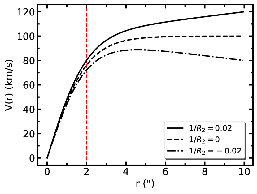
Figure 1: Example of rotation curve model. Each line shows different shape at the outskirt described by $1/R_{2}$ value (when $V_{\rm{ROT}}=100$ km/s and $R_{1}$=2${\arcsec}$) Vertical dotted line indicates $\rm R_{1}$.

3.1 Mock Galaxy Model

We define a mock galaxy model which resembles an actual rotating galaxy. Our mock galaxy is composed of simple photometric and kinematic models, which are flux distribution with the Sérsic profile and kinematic distribution with thin-disk approximated galaxy rotation curve (RC) function and a simple radial velocity dispersion function.

We use a model of galaxy with infinitely thin-disk shape and ordered rotation. There are several functional forms to describe the typical shape of the disk galaxies: an arc tangent (Puech et al., 2008), a hyperbolic tangent (Andersen & Bershady, 2013), and an inverted exponential (Feng & Gallo, 2011). All these model have a RC converging to a constant velocity at their outer radii, namely the well-known $flat$ rotation curve. Although it is non-trivial to describe the complex shape of the real RC in a simple form, we try to improve the current model while maintaining its simple form. We propose the following RC model which is a combination of the hyperbolic tangent function and a linear term,

$$V(r)=V_{\rm ROT}\;\Bigg{[}\rm tanh\Bigg{(}\frac{r}{R_{1}}\Bigg{)}+\frac{r}{R_{2}}\Bigg{]}$$ (2)

where $V_{\rm ROT}$ is a maximum circular velocity if $1/{R_{2}}=0$, $R_{1}$ is a characteristic radius where the curve slope changes, and $1/{R_{2}}$ is the slope of the curve at its outer radii. Figure 1 shows a few examples of this model with different signs of $1/{R_{2}}$. The advantage of this model is that it can describe the inclined/flat RC at the outer radii, as well as the rigid body rotation motion at near the center of galaxy, which are typically observed in the rotation curve of real galaxies. We would like to point out that there is a degeneracy between $R_{1}$ and $1/{R_{2}}$ in term of the shape of the curve. For example, the shape of RC model with certain $R_{1}=a$ and $1/{R_{2}}=b$ is identical to the other RC model with $R_{1}=ca$ and $1/{R_{2}}=b/c$. Therefore, to compare the shape of different set of our RC model parameters, a normalized RC outer radius, $R_{1}/{R_{2}}$, should be used.

Table 1: Mock IFU Data Parameters (Group 1 and 2)

Parameter	Value
IFU field of view ($\arcsec$)	32
IFU radial coverage in ${\rm{R}_{e}}$	2.5
S/N at 1${\rm{R}_{e}}$	10, 20, 30
Sérsic index	1, 4
Inclination ($\arcdeg$)	40, 55, 70
Position Angle ($\arcdeg$)	15
$V_{ROT}$ (km/s)	200
	3, -0.05
	3, 0.00
$R_{1}$ ($\arcsec$), $1/R_{2}$ ($1/\arcsec$)	3, 0.05
	2, 0.05
	4, 0.05
$\sigma_{0}$ (km/s)	150
$\sigma^{\prime}$	1
FWHM coefficient $c_{0}$ ($\arcsec$)	2.6 (Group 1)
	2.3, 2.6, 2.9 (Group 2)
FWHM coefficient $c_{1}$ ($\times 10^{-5}\;\arcsec/$Å)	-1.2
Redshift	0.02

Note. — S/N at 1 ${\rm{R}_{e}}$ is defined as median S/N of a spaxel around 1 ${\rm{R}_{e}}$ per spectral element.

We use a line-of-sight velocity dispersion function as follows,

$$\sigma_{r}=\frac{\sigma_{0}}{{\sigma^{\prime}}r/R_{1}+1},$$ (3)

where $\sigma_{0}$ is a velocity dispersion at the center, $r$ is a circular radial distance from the center of a galaxy, and $R_{1}$ is a characteristic scale which is set to be identical to the one in the RC model. The slope of $\sigma_{r}$ is mainly described by the $R_{1}$, but $\sigma^{\prime}$ is introduced to provide an additional freedom to the slope (subsection 5.1). The $\sigma_{r}$ form is taken from Graham et al. (2018) with slight modification, and it also well describes the actual velocity dispersion distribution of galaxies (see subsection 4.3).

Table 2: Mock IFU Data Parameters (Group 3)

Parameter	Value
IFU field of view (″)	12, 17, 22, 27, 32
IFU radial coverage in ${\rm{R}_{e}}$	1.5, 2.5
S/N at 1${\rm{R}_{e}}$	10 - 30
Sérsic index	1, 4
Inclination (°)	10 - 80
Position Angle (°)	15
$V_{ROT}$ (km/s)	50 - 300
$R_{1}$ (″)	1 - 4
$1/R_{2}$ (1/″)	-0.1 - 0.1
$\sigma_{0}$ (km/s)	50 - 300
$\sigma^{\prime}$	1
FWHM coefficient $c_{0}$ (″)	2.3 - 2.9
FWHM coefficient $c_{1}$ ($\times 10^{-5}$ ″/Å)	-3.6 - 1.2
Redshift	0.02

Note. — S/N at 1 ${\rm{R}_{e}}$ is defined as median S/N of a spaxel around 1 ${\rm{R}_{e}}$ per spectral element. When values of a parameter are listed with comma, one of the value is randomly selected. When values of a parameters is given in range (with hyphen), value is selected randomly within the range.

3.2 Mock IFU Data

We generate three $groups$ of mock IFS data using the fore-mentioned photometric and kinematic galaxy model. Each group of mock IFU data is determined by multiple $sets$ of model parameters, and each mock IFU data is generated to follow the two-dimensional velocity, velocity dispersion and flux distribution determined by a set of model parameters. The detail of mock IFU generation process is described in Appendix A. Here, we only describe the composition of each mock IFU data group.

The purpose of Group 1 is to investigate the performance of the deconvolution with respect to the number of deconvolution iterations. We determine sets of model parameters as in Table 1 to elaborate the diverse properties of galaxies. We use the realistic model parameters which could represent the photometric and kinematic distributions of actual galaxies such as the target galaxies of SDSS-IV MaNGA IFU survey. The S/N at one half-light radius (1 ${\rm{R}_{e}}$) is defined similarly to the MaNGA data, where ranges S/N=14-35 per spatial element per spectral resolution element in $r$ band at 1 ${\rm{R}_{e}}$ (Bundy et al., 2015). We also choose the shape and size of mock IFU field of view as same as the MaNGA IFU data, which has hexagonal shape with the field of view size of 12$\arcsec$ to 32$\arcsec$ in vertex to vertex with the size of spatial element as 0.5$\arcsec$ $\times$ 0.5$\arcsec$. Combination of each parameter; S/N at 1 ${\rm{R}_{e}}$, Sérsic index ($n_{S\acute{e}rsic}$), inclination angle, $R_{1}$, and $1/R_{2}$ yields 90 sets of mock galaxies ($3\times 2\times 3\times 5$ = 90) (see subsection 3.1 for the definition). For each set of galaxy parameters we construct three types of mock IFU data. Type 1 (Free) is an ideal IFU data without any PSF convolution or noise (i.e. free from atmospheric seeing effects and optical aberrations). Type 2 (Conv) is a realistic IFU data where Gaussian PSF is convolved and the Gaussian noise is added. Type 3 (Deconv) is a PSF-deconvolved IFU data which is obtained by performing the deconvolution method to the Type 2 IFU data. We generate 25 Conv IFU data from each Free mock IFU data by adding Gaussian random noise with 25 different random seeds. By using the distribution of the parameters measured from mock IFU data with different random noise, we obtain the statistical distribution of each extracted galaxy model parameters. Also, we assume the wavelength dependent $\rm{FWHM}_{\rm{PSF}}$ which corresponds to the $\rm{FWHM}_{\rm{PSF,\lambda}}=c_{0}+c_{1}\times\rm{\lambda}$, where $c_{0}$ and $c_{1}$ are as in the Table 1. This wavelength-dependent PSF is to represent the wavelength dependency of PSF in the real data (subsection 4.1). Lastly, 50 Deconv IFU data are produced per each Conv IFU data with $\rm{N}_{iter}$ = 1 to 50. In total, 90 Free, 2,250 Conv, and 112,500 Deconv mock IFU data are produced as Group 1.

Group 2 is designed to investigate the impact of the two types of $\rm{FWHM}_{\rm{PSF}}$ value to the performance of the deconvolution method; 1) $\rm{FWHM}_{\rm{Conv}}$ value which was convolved to the PSF-Free IFU mock data, and 2) $\rm{FWHM}_{\rm{Deconv}}$ value which is used for the deconvolution procedure. This is to verify the effect of deconvolution in practical situation where 1) each IFU data is observed with various atmospheric seeing size and 2) the $\rm{FWHM}_{\rm{Deconv}}$ being different from the actual effective $\rm{FWHM}_{\rm{Conv}}$. These effects are identified to ensure that the deconvolution provides more accurate kinematics compare to the one from the non-deconvolved data even with a little inaccurate $\rm{FWHM}_{\rm{Deconv}}$. We again construct three types of mock IFU data using the parameters given in Table 1. Group 2 - Type 1 data is identical to the Group 1 - Type 1 data. For each of the Group 2 - Type 1 Free IFU data, we produce 75 Conv IFU data by using 3 different $c_{0}$ values and the 25 different random noise seed per each $c_{0}$ value. 13 Deconv IFU data are produced per each Conv IFU data with 13 different $\rm{FWHM}_{\rm{Deconv}}$ values, which ranges within $\pm$ 0.3$\arcsec$ from the $c_{0}$ value with 0.05$\arcsec$ interval. $\rm{N}_{iter}$ is fixed as 20 times. In total, 90 Free, 6,750 Conv, and 87,750 Deconv mock IFU data are produced as Group 2.

Lastly, we produce Group 3 data using a range of mock galaxy model parameters as in Table 2. This is to verify the performance of deconvolution in more diverse combination of galaxy photometric and kinematic distributions. 40,000 sets of galaxy model parameters are determined randomly in Monte-Carlo way, and 1 Free, 1 Conv, 1 Deconv mock IFU are generated for each set. In total, 40,000 Free, 40,000 Conv, and 40,000 Deconv IFU data are produced as Group 3.

3.3 Kinematics Measurement and Rotation Curve Model Fitting

We measure the line-of-sight kinematics from the mock IFU data produced in subsection 3.2 and fit the RC model on the measured 2D kinematic distribution to extract the RC model parameter values. We use an IDL version of the Penalized-Pixel Fitting (pPXF)(Cappellari & Emsellem, 2004; Cappellari, 2017) procedure to extract the Line-Of-Sight-Velocity-Distribution (LOSVD) from the mock IFU data. To minimize the pPXF computation time, we use model SEDs identical to the ones that we used for the mock generation (see Appendix A), and fit only the velocity and the velocity dispersion without any additive or multiplicative Legendre polynomials or high-order kinematic moments. Following the recipe from Cappellari (2017), 1) we match the spectral resolution of the model SED to that of the mock IFU data, and 2) we de-redshift the mock IFU spectra to the rest frame before extracting the LOSVD. We also masked the wavelength around the known emission lines, although there is no emission line in the mock IFU spectra. Considering the wavelength coverage of the mock IFU data (3,540 to 7,410 Å; see Appendix A), we limit the fitting wavelength range as from 3700 to 7400 Å  for the LOSVD measurement.

We fit our RC model (Equation 2) to the extracted 2D velocity map of mock galaxies to quantify the shape of the rotation curve. From the fitting, we obtain the RC model parameters ($V_{ROT},R_{1},1/R_{2}$) and the kinematic geometrical parameters (center x, center y, position angle and inclination angle). The fitting procedure uses the minimum $\chi^{2}$ method that finds a set of parameters which is minimizing the $\chi^{2}$ between the true 2D velocity map and the measured 2D velocity map. The following equation describes the 2D model velocity map,

$$V_{\rm obs}(r^{\prime},\phi^{\prime})=V_{\rm SYS}+V(r)\;{\rm sin}\,i\;{\rm cos}(\phi-{\phi}_{0})$$ (4)

where $r^{\prime}$ is the distance from the kinematic center of the galaxy to each pixel on the sky, $r$ is galaxy-centric radius in the de-projected plane, $V_{\rm SYS}$ is a systematic line-of-sight velocity of the kinematic center, $i$ and $\phi_{0}$ are kinematic inclination angle and the position angle in the observed (projected) plane. Including the delta $\Delta$x and $\Delta$y from the kinematic center position in the observed plane, eight parameters are fitted simultaneously ($V_{SYS}$, $V_{ROT}$, $R_{1}$, $1/R_{2}$, $i$, $\phi_{0}$, $\Delta x_{cent}$, and $\Delta y_{cent}$).

The minimum $\chi^{2}$ method is sensitive to the initial values when there are multiple fitting parameters, in particular for the geometrical parameters ($i$, $\phi_{0}$, $\Delta x_{cent}$, and $\Delta y_{cent}$). To fit the 2D RC model with suitable initial parameter values, we first fit the 2D Sérsic model to the reconstructed $g$-band image of the mock IFUs before fitting the RC model. The geometrical parameters obtained from 2D Sérsic model are used as the initial value of the 2D RC model fitting.

There are two caveats in fitting our RC model.

1. The velocity map should cover sufficiently large radial range along the major axis compare to the $R_{1}$, otherwise the $1/R_{2}$ parameter cannot be accurately determined. In particular, it is important to have sufficient radial coverage along the major axis. The radial coverage along the minor axis contributes significantly less than the coverage along the major axis to the RC model fitting, because of the ${\rm cos}(\phi-{\phi}_{0})$ term in Equation 4.

2. The 2D RC model is less sensitive to the galaxies with too low or too high inclination angle. Due to the ${\rm sin}\,i$ term in the Equation 4, $V_{ROT}$ term is often inaccurately measured at low inclination angle (close to face on). At high inclination angle, the fitting result is not reliable because of the relatively small number of data points along the major axis, and the significant PSF convolution effects which scrambles the information between the measured quantities on and out of the major axis, even in the PSF-deconvolved mock IFU data.

In Appendix B, we analyze the RC model fitting result of the Group 3 mock IFU data and derive analytic criteria to ensure the accuracy of the RC model fitting result. We find that when the result satisfies $R_{max,S/N>3,major}/R_{1}>2.5$ and the fitted inclination angle falls on $75\arcdeg>i>25\arcdeg$, the fitting results are considered reliable. In addition, we find that the model parameter values measured from the mock IFU data with field of view equal to 12$\arcsec$ are not well recovered because of insufficient number of valid data points (S/N $>$ 3) in such a narrow field of view with a given spatial element size (0.5$\arcsec$ by 0.5 $\arcsec$). In further analysis, we only consider the fitting results those are satisfying the above criteria ($R_{max,S/N>3}^{major}/R_{1}>2.5$ and $75\arcdeg>i>25\arcdeg$).

3.4 Results and Discussion

In this subsection, we present the performance of our deconvolution method by using the mock IFU data. We show the relation between the restored kinematics and the deconvolution parameters ($\rm{N}_{iter}$, $\rm{FWHM}_{\rm{Deconv}}$) and discuss the adequate choice of the deconvolution parameters. Lastly, we demonstrate the feasibility of applying our deconvolution method to more generalized cases, by showing the test result of the deconvolution method to mock IFU data with various combination of the galaxy surface brightness distribution, galaxy inner and the outer kinematics, its geometry, radial coverage and S/N of data, geometry, and size of the convolved PSF size.

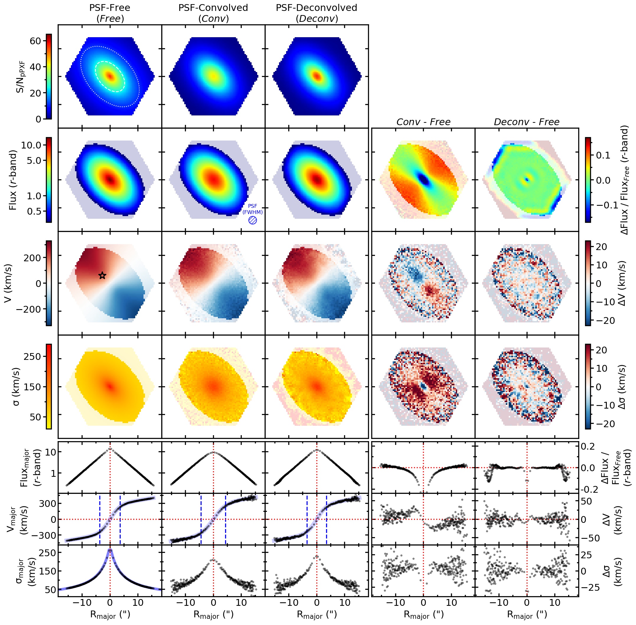
Figure 2: Plots demonstrating the effects of the PSF convolution and deconvolution on the 2D maps of S/N, $r$-band flux, line of sight velocity (V), and velocity dispersion ($\sigma$). 1D radial profiles of the $r$-band flux, line of sight velocity, and velocity dispersion along the major-axis are also shown. The first, second, and third column represent the 2D or 1D distribution of the measured quantities from PSF-Free (Free), PSF-Convolved (Conv), and PSF-Deconvolved (Deconv) mock IFU data. The mock IFU data is selected from Group 3 Monte-Carlo mock IFU samples (see text). The fourth (fifth) column show the difference between the quantities from the Conv (Deconv) and the Free mock IFU data, respectively. The size of the major tick in the 2D maps is 10$\arcsec$. A dashed (dotted) ellipse is over-plotted on the top left corner panel to represent the size of 1$R_{e}$ (2$R_{e}$). FWHM of the convolved PSF is shown as a blue hatched circle in the Flux - Conv panel. Black open star on V - Free panel is the location of the example spectrum in Figure 3. Spaxels with S/N $<$ 3 are paled out in the 2D maps except for the S/N map. Only data points within $\pm 5\arcdeg$ of major axis are shown in the radial profiles for clarity. Blue paled-out lines are under-plotted on the $V_{major}$ profiles ($\textit{Free},\textit{Conv},\textit{Deconv}$) and the $\sigma_{major}$ profile (Free only) to represent the fitted RC (and $\sigma$) model functions. Blue vertical dashed lines in the $V_{major}$ profiles denote $R_{1}$ of the corresponding fitted RC model function.

3.4.1 Effects of PSF Convolution and Deconvolution

Figure 2 shows the effects of PSF convolution and deconvolution by using test result from one of the Group 3 (Monte-Carlo) mock IFU data ($n_{S\acute{e}rsic}=1$, ${S/N}_{1{\rm{R}_{e}}}=25$, $i=48\arcdeg$, $V_{ROT}$=212 km/s, $R_{1}$=3.7$\arcsec$, $1/R_{2}$=0.02 (1/$\arcsec$), $\sigma$=74 km/s, $\rm FWHM_{PSF}$=2.88$\arcsec$, field of view = 32$\arcsec$). Panels on the leftmost column show the 2D or 1D quantities measured or extracted from the Free IFU data. The quantities match very well with the model 2D photometric and kinematic distributions which we put into, meaning that the mock IFU data is constructed accurately in accordance with the model parameters. The second left column presents distributions from Conv IFU data, and the second right column displays the difference between the leftmost and the second left column.

As expected, the panels clearly exhibit noticeable changes in all three quantities (flux, velocity, and the velocity dispersion) caused by the PSF convolution. The difference in $\rm{Flux}_{major}$ and $\rm{V}_{major}$ 1D profiles (the second right column) also show evident deviation between the Conv and the Free. In particular, the characteristic radius of the rotation curve ($R_{1}$, represents the size of the inner linear part) is increased by the PSF convolution. The overall velocity dispersion around the center is also increased, but at the very center the dispersion is decreased. This is caused by the combination of the PSF convolution effects on the line-of-sight (LOS) velocity, and the velocity dispersion distribution. The convolved PSF increases the velocity dispersion, in particular along the minor axis because of the the opposite direction of LOS velocity around the minor axis. On the other hand, the convolved PSF smooths the velocity dispersion distribution so that it decreases the velocity dispersion at the center but increases the dispersion around the center because the center has both the brightest point and the highest velocity dispersion.

The central column presents the distributions from Deconv IFU data, and the rightmost column shows the difference between the Deconv and Free. It is clear that the difference between the Deconv and the Free is significantly less than the same between the Conv and the Free. Compare to the Conv column, the apparent b/a ratio is decreased, the flux at the center is increased, and the $\rm R_{1}$ of the rotation curve is now much closer to the one from the Free column. The difference in both velocity and velocity dispersion distribution is also much diminished. This result clearly exhibits that the flux, velocity, and the velocity dispersion distribution from the PSF-deconvolved IFU data are indeed well-recovered toward the true distributions. However, the distribution near the edge of the galaxy becomes fuzzier and shows some systematic feature, in particular in the flux distribution. This is partially due to the low S/N near the edge of mock IFU data, and partially due to the edge effect of the deconvolution. We would like to point out that the edge effect in this example is already significantly reduced by the iterative value-correction process (see subsection 2.2). Without the iterative value-correction process, the edge effect makes distinctive artificial hexagonal shape oscillating pattern on the entire image. We put additional examples of Group 1 mock IFU data in Appendix C to show the result with different input distributions. The examples in Appendix C demonstrate that the deconvolution method on IFU data is working effectively well and the method restores the distributions of photometric and kinematic quantities close to the true distributions.

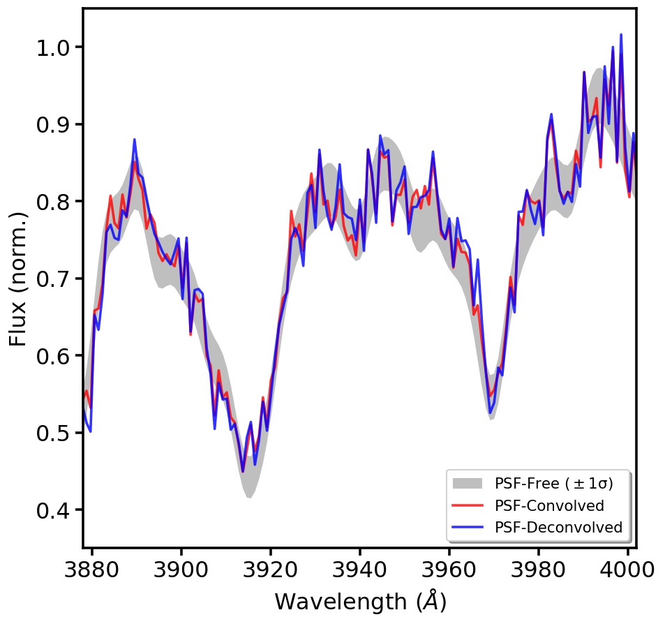
Figure 3: Spectrum of a spaxel whose $\Delta V$ between the Conv and the Free is -20 km/s. Only the spectra around the Ca H&K lines are shown. The location of this spaxel is marked as a black open star in Figure 2. Median S/N of this spaxel is 36. Each spectrum is normalized by the median of each to show only the difference between spectra in their shape. The thickness of the spectrum from Free (grey) represents $\pm 1\sigma$ error at each wavelength bin.

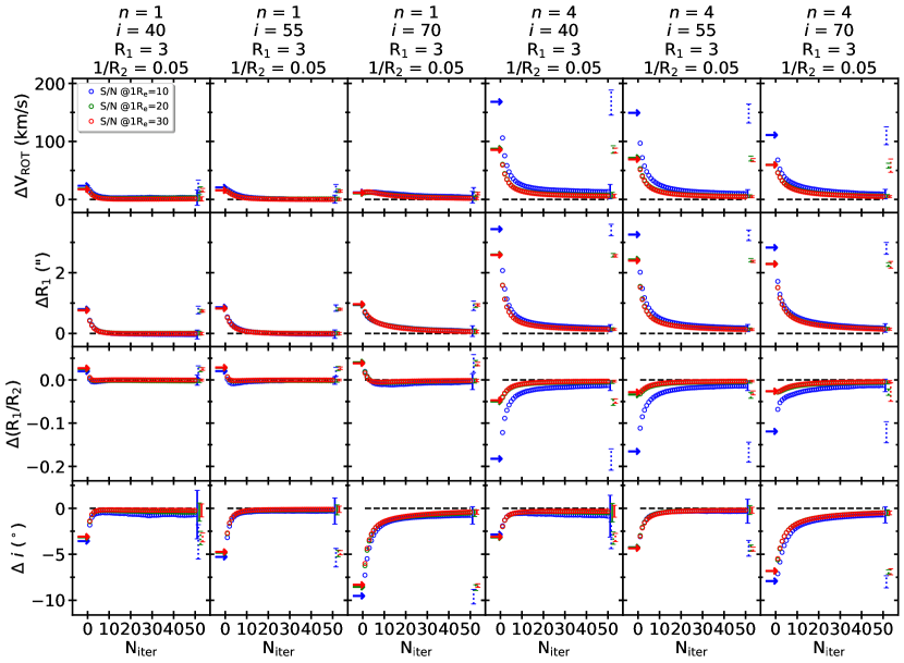
Figure 4: Difference between the true RC model parameters and the fitted model RC parameters from the PSF-deconvolved mock data (Deconv) with respect to the number of LR deconvolution iteration ($\rm{N}_{iter}$ = 1 to 50). Each column shows the results from the mock IFU data with different Sérsic index ($n_{S\acute{e}rsic}$) and kinematic inclination angle ($i$). In each panel, $\rm\Delta$ of one of the four RC model parameters ($\rm\Delta{V}_{ROT},\Delta{R}_{1},\Delta({R}_{1}/{R}_{2})$, and $\rm\Delta{i}$) with different number of deconvolution iteration ($\rm{N}_{iter}$) are plotted as open circles. Color represents the S/N at 1 ${\rm{R}_{e}}$ value that is used to generate the corresponding PSF-free mock IFU data (Free) of each open circle. Black dashed lines are plotted at the difference of 0 as a guidance. Arrow points out the value of the fitted parameters from the PSF-convolved mock IFU data (Conv). For clarification, we put only one solid error bar per S/N at 1 ${\rm{R}_{e}}$ value in each panel instead of putting error bars on every open circles. The error bar represents the standard deviation of each $\rm\Delta$ parameter values from 25 different random seeds (There is almost no dependency of the standard deviation of the $\rm\Delta$ parameters with respect to $\rm{N}_{iter}$). The dotted error bar is corresponding standard deviation from the difference between the true RC model parameter value and the fitted model RC parameter value of the PSF-convolved (Conv) mock IFU data.

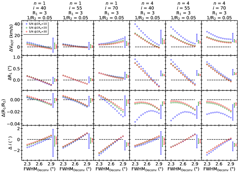
Figure 5: Difference between the true RC model parameters and the fitted model RC parameters from the PSF-deconvolved mock data (Deconv) with respect to the FWHM of PSF used for the deconvolution (with fixed $\rm{N}_{iter}=20$). Each column shows the results from the mock IFU data with different Sérsic index ($n_{S\acute{e}rsic}$) and kinematic inclination angle ($i$). In each panel, $\rm\Delta$ of one of the four RC model parameters ($\rm\Delta{V}_{ROT},\Delta{R}_{1},\Delta({R}_{1}/{R}_{2})$, and $\rm\Delta{i}$) with different PSF FWHM size used for the deconvolution ($\rm{FWHM}_{\rm{Deconv}}$) are plotted as open circles. Color represents the S/N at 1 ${\rm{R}_{e}}$ value that is used to generate the corresponding PSF-free mock IFU data (Free) of each open circle. Again, black dashed lines are plotted at the difference of 0 as a guidance. For clarification, we put only one solid error bar per S/N at 1 ${\rm{R}_{e}}$ value in each panel instead of putting error bars on every open circles. The solid error bar represents the standard deviation of each $\rm\Delta$ parameter values from 25 different random seeds, as in Figure 4 (There is almost no dependency of the standard deviation of the $\rm\Delta$ parameters with respect to $\rm{FWHM}_{\rm{Deconv}}$). Note that y-axis scale of in this figure is smaller than that of Figure 4.

We visualize the effect of the deconvolution method in the wavelength dimension in Figure 3. Figure 3 shows an example of spectra at the spaxel where $\Delta V$ between the Conv and the Free is about -20 km/s. Because the size of one wavelength bin of the spectrum corresponds to 69 km/s, $\Delta V$ of -20 km/s ($\sim$0.29 pixel) is hardly recognized between the spectra by eyes, even around the strong absorption lines. It is also noticed that the Deconv spectrum is slightly noisier than the Conv spectrum. The mean difference between the Conv and the Free spectrum at this spaxel is 4.0%, but the corresponding difference between the Deconv and the Free spectrum is 4.6%. In fact, the noisier Deconv spectrum is expected by the effect of LR deconvolution algorithm (noise amplification). Although the Deconv spectrum is noisier than the Conv spectrum, the overall shape of the Conv spectrum has changed and shifted through the deconvolution process, and the line-of-sight velocity and the velocity dispersion of the Deconv spectrum are better recovered to the true value.

3.4.2 Deconvolution Parameters

Figure 4 represents the difference between the fitted and the true RC model parameter value as $\rm{N}_{iter}$ increases from 1 to 50. Error bar is calculated from the 25 mock IFU data with different random seeds which we implemented for the noise realization. Since the deviation from the true value depends on the galaxy model parameters, we show the result from multiple model galaxies at each column from the Group 1 mock IFU data. The figure shows the case of the mock data with $n_{S\acute{e}rsic}$ = 1, 4 and $i$ = 40, 55, 70$\arcdeg$. Here we present the difference in $R_{1}/R_{2}$ rather than $1/R_{2}$, because $R_{1}/R_{2}$ value better describes the overall shape of rotation curve without degeneracy (see subsection 3.1).

It is evident that the difference between fitted RC model parameter values measured from the Deconv and the true RC model parameter decreases $\rm{N}_{iter}$ increases. Although the difference does not converge to zero it is clear that the difference is significantly reduced by the deconvolution method. Note that the size of $\rm 1\sigma$ error of the fitted RC model parameter values from Deconv is smaller than the $\rm\Delta$ between the parameter values measured from Conv and the true values. This result clearly exhibits that the kinematic parameters are reasonably well-restored closely to the true values, even considering the measurement error.

To visualize the effect of $\rm{N}_{iter}$, we show varying 2D $r$-band flux, line of sight velocity, and velocity dispersion map as $\rm{N}_{iter}$ changes in Figure D.1, using the same mock IFU data as in the Figure 2. Note that the variation is shown for selected $\rm{N}_{iter}$ = 0 (Conv; No deconvolution), 1, 2, 3, 10, 20, and 30. Similar to the trend of difference between the true RC model parameters and the fitted model RC parameters to $\rm{N}_{iter}$ (Figure 4), the amount of difference between 2D map from true and deconvolved IFU data is larger for the small $\rm{N}_{iter}$.

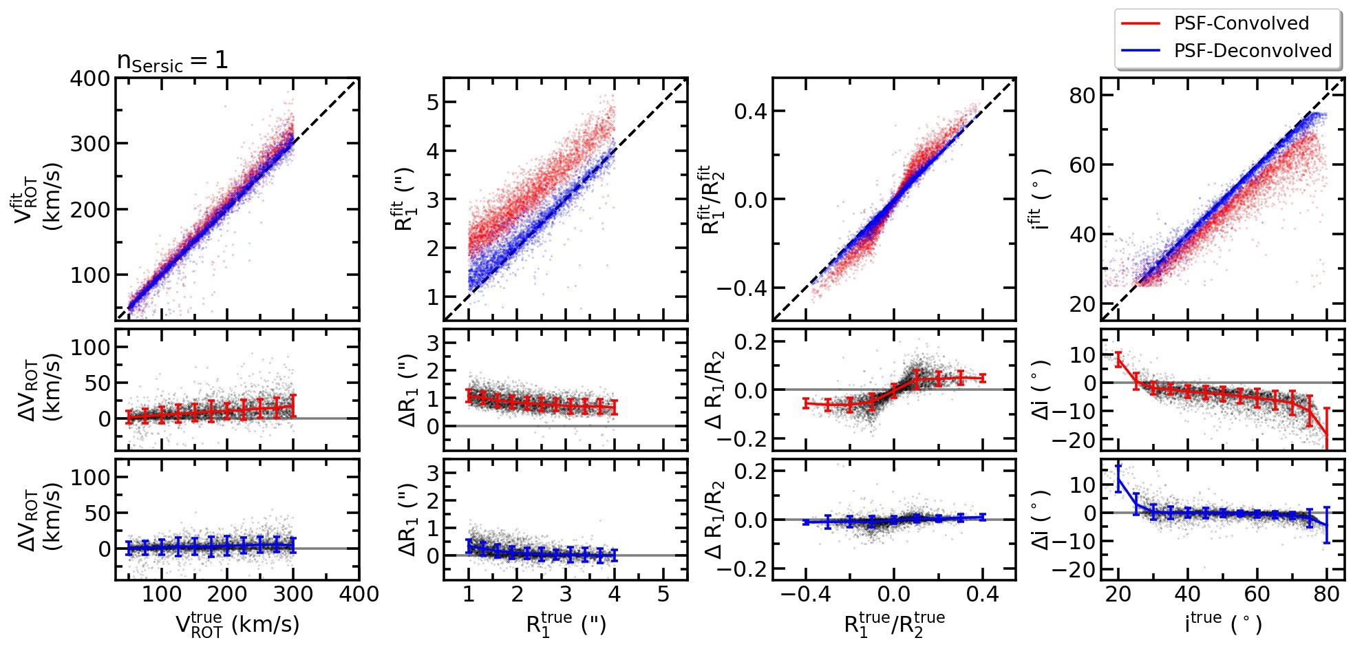
Figure 6: Top panel of each column shows 1:1 relation between the fitted RC model parameter values from Conv IFU data and the true parameter value (red), and the relation between the fitted RC model parameter values from Deconv IFU data and the true value (blue), when $n_{S\acute{e}rsic}=1$. Middle (bottom) panel of each column presents the difference between the fitted RC model parameter values from Conv (Deconv) IFU data and the true value with respect to the true parameter values. The error bar in the middle and the bottom panel shows the 1-$\sigma$ range of the data points within each arbitrary bin size.

In subsection D.1, we present additional similar figures with various mock galaxy model parameters to support the validity of our deconvolution method.

Figure 5 presents the difference between the fitted RC model parameter and the respective true value as a function of the Gaussian PSF FWHM used for the deconvolution ($\rm{FWHM}_{\rm{Deconv}}$). $\rm{FWHM}_{\rm{Deconv}}$ is varied from 2.3$\arcsec$ to 2.9$\arcsec$ with 0.05$\arcsec$ increment when the FWHM of the convolved Gaussian PSF ($\rm{FWHM}_{\rm{Conv}}$) is $2.6\arcsec$. $\rm{N}_{iter}$ is fixed as 20. Again the error is calculated from the result with 25 mock IFU data generated with different random seeds. The figure shows the case of the mock IFU data with the combination of $n_{S\acute{e}rsic}$ = 1, 4 and $i$ = 40, 55, 70$\arcdeg$ with fixed $R_{1}$ and $1/{R_{2}}$ as 3 and 0.05. Indeed there is a dependency of the fitted parameters to the $\rm{FWHM}_{\rm{Deconv}}$ value, but variation of the value is not significant when the $|\rm{FWHM}_{\rm{Deconv}}-\rm{FWHM}_{\rm{Conv}}|<0.3\arcsec$, considering the error bar. As the $\rm{FWHM}_{\rm{Deconv}}$ is varied, the difference between the parameters from the Deconv (open circles) to the true value changes but not always linearly. In all cases, the measured parameter values from the deconvolved IFU data are clearly getting closer to the true value, compare to the values without deconvolution (values measured from Conv mock IFU data). Considering all four kinds of fitted parameters, the best result is obtained when $\rm{FWHM}_{\rm{Deconv}}=\rm{FWHM}_{\rm{Conv}}$, although the difference between the fitted and the true model parameters from the Deconv and the Free are not always minimum at $\rm{FWHM}_{\rm{Deconv}}=\rm{FWHM}_{\rm{Conv}}$. From this test result, we conclude that in most cases, the deconvolved IFU data produces fairly consistent result when the $\rm{FWHM}_{\rm{Deconv}}-\rm{FWHM}_{\rm{Conv}}$ is less than $0.3\arcsec$ (i.e. when the measurement error of the size of $\rm{FWHM}_{\rm{Conv}}$ is less than $0.3\arcsec$). In subsection D.2, we present supplementary figures with different $\rm{FWHM}_{\rm{Conv}}$ values ($2.3\arcsec$ and $2.9\arcsec$) and different mock galaxy model parameters.

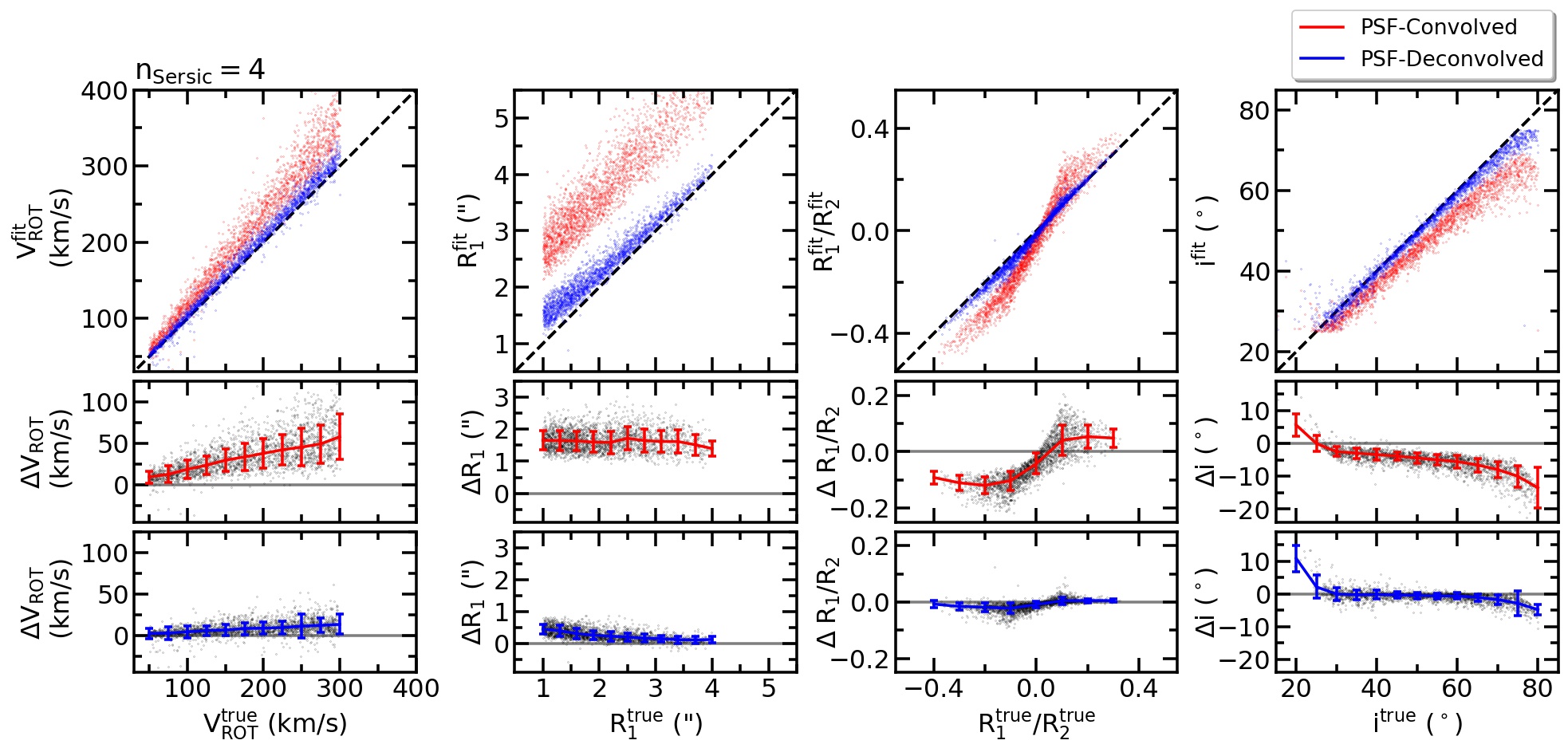
Figure 7: Same as Figure 6 but with mock IFU data of $n_{S\acute{e}rsic}=4$

3.4.3 Results from the Monte-Carlo Mock IFU data

Here we present the result of the deconvolution method performance verification test with Group 3 Monte-Carlo mock IFU data. This is to validate that the deconvolution method works well not only with the mock galaxy model with certain combination of model parameter values, but also with diverse combination of the galaxy model parameters. We divide the results according to $n_{S\acute{e}rsic}$ value because the results are highly correlated with $n_{S\acute{e}rsic}$. Figure 6 and Figure 7 shows the results with $n_{S\acute{e}rsic}=1$ and $n_{S\acute{e}rsic}=4$, respectively. Note that we only include the results when the Deconv mock IFU data satisfies the fitting qualification criteria, which are IFU field of view equal or wider than 17$\arcsec$, $R_{major,S/N>3}$/$R_{1}>2.5$, and $75\arcdeg>i>25\arcdeg$. The number of mock IFU data used for Figure 6 is 2,354, and for Figure 7 is 3,820. In Figure 6, all $V_{ROT}$, $R_{1}$, ${R}_{1}/{R}_{2}$ and $i$ model parameters measured from the Deconv mock IFU data show good agreement with the true value. On the contrary, the model parameter values measured from Conv mock IFU data show considerable deviations from the true value. In Figure 7, again all parameters measured from the Deconv mock IFU data show good agreement with the true value. The model parameter values measured from Conv mock IFU data show larger discrepancy in the case of $n_{S\acute{e}rsic}=4$.

Figure 8: (left) Distribution of the reconstructed FWHM in $g$-band. Median value is 2.53$\arcsec$. (middle) Wavelength-dependent $\rm{FWHM}_{\rm{PSF}}$ of the selected MaNGA galaxies. Each connected line represents $griz$ FWHM of PSF from a particular sample. Samples are randomly selected for illustrative purpose. Error bar shows $\rm\pm$0.025$\arcsec$ range (1% of 2.5$\arcsec$). (right) Distribution of wavelength-dependent FWHM gradient. The gradient is obtained by fitting a linear function to the reconstructed FWHM at $griz$-bands. Median value is $-1.21\times 10^{-5}\arcsec/$Å.

Results from the figures show that our deconvolution method successfully restores the kinematic properties of galaxies. It also shows that the measured parameter values from the Conv mock IFU data have a noticeable deviation from the true value, especially when $n_{S\acute{e}rsic}=4$. It can be interpreted as the PSF convolution effect becomes more significant when there is a steeper relative flux slope between the adjacent spaxels. This effect is most evident for $R_{1}$ parameter. $R_{1}^{fit}-R_{1}^{true}$ of the Conv mock IFU data show a median offset of 1.8 $\arcsec$ in Figure 7. This large offset also affects $1/R_{2}$, where many $1/R_{2}$ values from Conv are measured in the condition where they did not meet the fitting qualification criteria.

4 Application to SDSS-IV MaNGA IFU Data

4.1 MaNGA Point Spread Function

We use IFU data from the third public release of the MaNGA (Bundy et al., 2015), that is a part of SDSS DR15 (Aguado et al., 2019). Among the 4,824 DR15 MaNGA cube data, we select 4,426 unique galaxies from the MaNGA main galaxy sample (Primary, Color-enhanced primary, and secondary; Wake et al. (2017)) by removing repeated observations, duplicated galaxies with different MaNGA-ID , and special targets (IC342, Coma, and M31). For the repeated observations and duplicated galaxies, we choose data observed by a bigger IFU. If both are observed by IFU with the same size, then we use the data with higher blue channel S/N as recorded in the FITS header of the data. In the context of deconvolution, it is important to know the accurate information about the shape and size of PSF that is convolved to each MaNGA IFU data. According to Law et al. (2015, 2016); Yan et al. (2016), it is known that 1) size of PSF FWHM ranges between 2.2$\arcsec$ and 2.7$\arcsec$ in $g$-band, 2) shape of PSF is well-described by a single 2D circular Gaussian function, 3) FWHM of the fitted model Gaussian function agrees with the measured FWHM within 1 - 2%, 4) PSF FWHM varies less than 10% across the field of view within a single MaNGA IFU. MaNGA IFU data provides the reconstructed MaNGA PSF image in $griz$ band as well as $griz$ PSF FWHM values in its header. The $g$-band PSF FWHM distribution of the entire SDSS DR15 MaNGA data is shown in the left panel of Figure 8. To account for the wavelength dependency of MaNGA PSF FWHM (Figure 8, middle panel), we fit a simple linear function (first order polynomial) to the PSF FWHM of $griz$-bands to interpolate/extrapolate the PSF FWHM value at other wavelengths. The average absolute difference between the reconstructed PSF FWHM values recorded in the IFU data header and the PSF FWHM values from the fitted linear function is 0.007$\arcsec$ with standard deviation of 0.006$\arcsec$, calculated from the entire MaNGA IFU data.

Considering the error of the reconstructed PSF FWHM of MaNGA IFU data (1-2% or 0.025-0.05 in arcsec)(Law et al., 2016), we conclude that the PSF FWHM from the fitted linear function gives reasonable PSF FWHM at each wavelength bin. The distribution of the slope of the fitted linear functions is shown in the right panel of Figure 8.

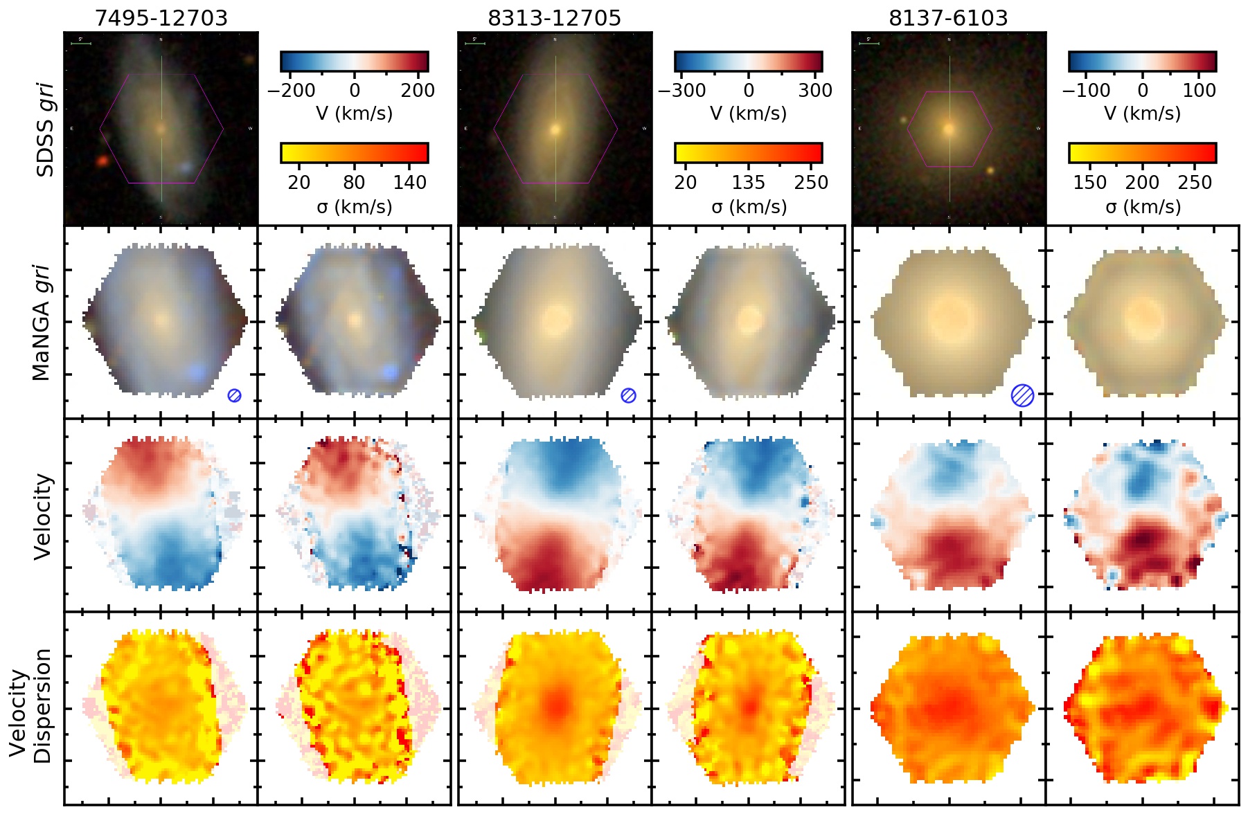
Figure 9: The results of the PSF deconvolution on three MaNGA galaxies. The number at the top of each SDSS $gri$ image is the PLATE-IFU designation of a given galaxy. For each galaxy, images in the left column show reconstructed MaNGA gri image, velocity and velocity dispersion distribution obtained from the $original$ MaNGA data. Images in the right column are those from the PSF-deconvolved MaNGA data. Hatched blue circle represents PSF FWHM size of each galaxy. Spaxels with median ${\rm S/N}_{\rm pPXF}<$ 3 are paled out in the velocity and velocity dispersion distributions. Each major tick interval corresponds to 10$\arcsec$.

4.2 Measurements of Kinematic Parameters

We measure the line-of-sight velocity and the velocity dispersion from 4,425 unique MaNGA galaxies. The measurement procedure is similar to the procedure that is described in subsection 3.3, but with several differences. Instead of using one single-stellar population model template, we use 156 single-stellar population model SED templates from MILES stellar library (Sánchez-Blázquez et al., 2006; Falcón-Barroso et al., 2011; Vazdekis et al., 2010) generated by using unimodal initial mass function (Vazdekis et al., 1996) and Padova+00 isochrones (Girardi et al., 2000), age from 1 to 17.78 Gyr, and metallicity (Z) from -2.32 to 0.22 (26 ages $\times$ 6 metallicites = 156). We use an option to use 6^th order additive and multiplicative Legendre polynomials during the fitting to account for the low-order difference and offset between the MILES model and data. We mask the spectrum pixels around the known emission lines. Model SED templates are convolved with a Gaussian function to match the spectrum resolution of MaNGA data as provided in the SPECRES HDU.

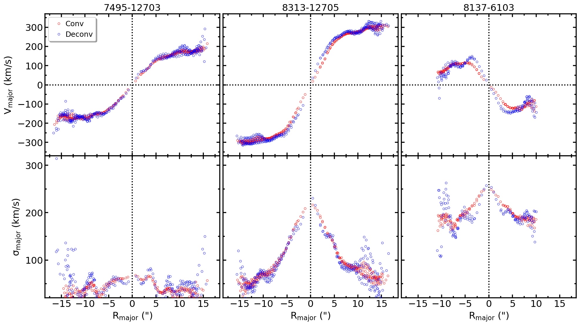
Figure 10: The velocity and velocity dispersion profiles from the original and deconvolved MaNGA data. Only the data points from $\pm 10\arcdeg$ of the major axis with median ${\rm S/N}_{\rm pPXF}>3$ are shown for clarity.

4.3 Results

Figure 9 shows the result of deconvolution applied to the three of the MaNGA galaxies as an example (PLATE-IFU: 7495-12703, 8313-12705, 8137-6103). These galaxies are chosen based on their shape of the rotation curve and the velocity dispersion profile. Each reconstructed $gri$ image obtained from the deconvolved MaNGA ($Deconv$) data shows a noticeable difference compare to the reconstructed $gri$ image from the original MaNGA ($Ori$) data. The MaNGA-$Deconv$ data shows more sharpened substructures. The restored substructures are not artifacts created by the deconvolution method but are actual substructures which can be seen in the SDSS $gri$ image that has higher spatial resolution. The velocity distribution also shows the apparent change, especially around the center of galaxies (i.e. the velocity gradient becomes steeper). The velocity dispersion exhibits some changes as well, and shows narrower dispersion distribution near the center and sharper substructures. The restored substructures can be understood intuitively as a result of deconvolution. The difference between MaNGA-$Ori$ and MaNGA-Deconv data can be seen more prominently in Figure 10. The figure clearly exhibits the changes in the velocity and the velocity dispersion distribution along the galaxy major axis.

5 Measurement of the Spin Parameter

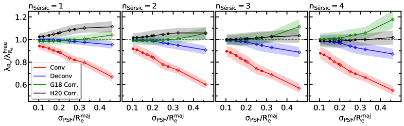
Figure 11: Ratio between the true and the measured/corrected spin parameter $\lambda_{R_{e}}$ depending on $n_{S\acute{e}rsic}$ and $\rm\sigma_{PSF}/R_{e}^{maj.}$. The left most panel shows the ratio measured from the Group 3 mock IFU data (Table 2) with $n_{S\acute{e}rsic}=1$. Other panels show the result from mock IFU data with $n_{S\acute{e}rsic}$= 2, 3, 4. Filled-circle points are estimated from mock IFU data with radial coverage = 1.5 $\rm{\rm{R}_{e}}$, and the open-diamond points are estimated from mock IFU data with IFU radial coverage = 2.5 $\rm{\rm{R}_{e}}$.

In this section, we investigate the reliability of the $\lambda_{R}$ parameter measured from the deconvolved IFU data. $\lambda_{R}$ is a proxy of the spin parameter $\lambda$. It is calculated from the luminosity-weighted first and second velocity moments as in Emsellem et al. (2007),

$$\lambda_{R}\equiv\frac{\langle R|V|\rangle}{\langle R\sqrt{V^{2}+\sigma^{2}}\rangle}=\frac{\Sigma^{N}_{i=1}F_{i}R_{i}|V_{i}|}{\Sigma^{N}_{i=1}F_{i}R_{i}\sqrt{V_{i}^{2}+\sigma_{i}^{2}}},$$ (5)

where $F_{i},R_{i},V_{i},\sigma_{i}$ are flux, radius of the concentric ellipse, line-of-sight velocity and line-of-sight velocity dispersion at the $i$th spatial bin, respectively. $\lambda_{R}$ is widely used in various applications, such as kinematic classification of galaxies (Emsellem et al., 2011; van de Sande et al., 2017; Cortese et al., 2016; Graham et al., 2018), measurement of the angular momentum of merger remnants (Jesseit et al., 2009), and the studies of the environmental dependence of galaxy spin (Greene et al., 2018; Lee et al., 2018).

Typically $\lambda_{R}$ is calculated by using the information within galaxy half-light radius (equivalent to the $R_{e}^{major}$)(Hopkins et al., 2010; Cappellari et al., 2013), and denoted as $\lambda_{R_{e}}$. It is known that $\lambda_{R_{e}}$ is mainly correlated with two parameters: inclination angle ($\epsilon$, as axis ratio) and FWHM of PSF that is convolved in data, because distribution of $F_{i},R_{i},V_{i}$, and $\sigma_{i}$ are much affected by those parameters (Cappellari, 2016; Graham et al., 2018).

There were several attempts to mitigate the effect of the PSF on $\lambda_{R_{e}}$ measurement: 1) by correcting $\lambda_{R_{e}}$ by 1/$\sqrt{\epsilon}$ (Emsellem et al., 2011; D’Eugenio et al., 2013; Cortese et al., 2016; Greene et al., 2018) or 2) by applying an empirical correction function such as Graham et al. (2018)(hereafter G18) and Harborne et al. (2020)(hereafter H20).

Here we show that our deconvolution method can also be used to accurately measure $\lambda_{R_{e}}$. In subsection 5.1, we measure $\lambda_{R_{e}}$ from the Group 3 Monte-Carlo mock IFU data (Free, Conv, Deconv) and compare the $\lambda_{R_{e}}$ measured from each type of the mock IFU data. From the result, we find that the $\lambda_{R_{e}}$ value measured from the deconvolved IFU data is close to the true $\lambda_{R_{e}}$. In subsection 5.2, we measure $\lambda_{R_{e}}$ from both MaNGA-$Ori$ and MaNGA-$Deconv$, and examine the differences.

5.1 Verification using Mock Data

We calculate $\lambda_{R_{e}}$ following Equation 5, by using the reconstructed $r$-band flux, the velocity and the velocity dispersion distribution measured from the Free, Conv, Deconv Monte-Carlo mock IFU data (Group 3, 40,000 IFU data each)(see subsection 3.2 and Table 2). each spaxel is calculated from the geometrical parameter of the Free mock IFU data. We also calculate the corrected $\lambda_{R_{e}}$ value by applying the correction function in G18 to $\lambda_{R_{e}}^{Conv}$ value to compare the result between the corrected value and the value measured from the deconvolved IFU data. To apply correction function of G18 and H20, we use $n_{S\acute{e}rsic}^{Free}$, $R_{e}^{Free}$ and $\rm{FWHM}_{\rm{PSF}}$ at the $r$-band pivot wavelength (6231Å). $R_{e}^{Free}$ should be used instead of $R_{e}^{Conv}$.

First, we check the ratio between the calculated $\lambda_{R_{e}}$ values ($\lambda_{R_{e}}^{Conv}$, $\lambda_{R_{e}}^{Deconv}$, $\lambda_{R_{e}}^{G18\;Corr.}$, and $\lambda_{R_{e}}^{H20\;Corr.}$) and the true $\lambda_{R_{e}}$ value ($\lambda_{R_{e}}^{Free}$), as a function of true $\lambda_{R_{e}}^{Free}$ value. In our mock IFU data, the angular size of ${\rm{R}_{e}}$ is determined by the combination of IFU FoV and radial coverage in ${\rm{R}_{e}}$ (Table 2, Appendix A). Thus, we divide the result depending on three parameters of mock IFU data, 1) $n_{S\acute{e}rsic}$ (1, 2, 3, 4), 2) IFU FoV (12$\arcsec$ to 32 $\arcsec$), and 3) radial coverage in ${\rm{R}_{e}}$ (1.5 ${\rm{R}_{e}}$ and 2.5 ${\rm{R}_{e}}$). We plot the relation between the calculated ratios to the $\lambda_{R_{e}}^{Free}$ of each divided result. Figure E.1 is shown as an example of the result for the mock IFU data with $n_{S\acute{e}rsic}$=1 and 4, and IFU FoV = 1.5 ${\rm{R}_{e}}$ and 2.5 ${\rm{R}_{e}}$. To illustrate the overall dependence of the ratio to the $n_{S\acute{e}rsic}$ and the size of ${\rm{R}_{e}}$, we take the median of the ratios and the median of the standard deviation of the ratios at each bin (per $\rm\Delta\lambda_{R_{e}}^{Free}$=0.1) in each panel of Figure E.1. For example, the right most filled-circle red data point in the left most panel in Figure 11 ($\rm\sigma_{PSF}$/${\rm{R}_{e}}^{maj}=0.276$, $\lambda_{R_{e}}^{Conv}/\lambda_{R_{e}}^{Free}$=$\rm 0.82\pm 0.03$)) is derived from the top left panel of Figure E.1 ($n_{S\acute{e}rsic}=1$, IFU FoV=12$\arcsec$ (=1.5 ${\rm{R}_{e}}$)) by taking the median and the median of $\rm 1\sigma$ of the binned relation. Note that the actual $\rm\sigma_{PSF}$/${\rm{R}_{e}}^{maj}$ of each combination of IFU FoV and the radial coverage is not a constant. This is because $\rm FWHM_{PSF}$ of the Group 3 IFU data is slightly different for each mock IFU data as 2.6 $\pm$ 0.3$\arcsec$. Since ${\rm{R}_{e}}$ is different for each combination of IFU FoV and the radial coverage, the difference caused by $\rm FWHM_{PSF}$ is also different for each combination of IFU FoV and the radial coverage (e.g. $\rm\Delta(\sigma_{PSF}/{\rm{R}_{e}}^{maj})=\pm 0.04$ for IFU FoV=12$\arcsec$ and radial coverage=2.5${\rm{R}_{e}}$). Nevertheless, Figure 11 could still be used to show the dependence of $\lambda_{R_{e}}^{Conv}/\lambda_{R_{e}}^{Free}$ with respect to $\rm\sigma_{PSF}$/${\rm{R}_{e}}^{maj}$.

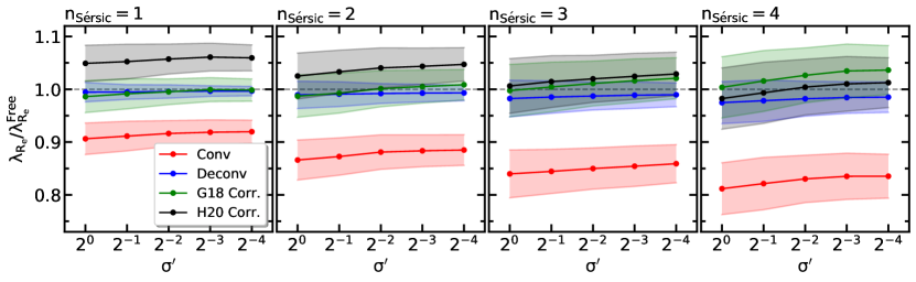
Figure 12: Ratio between the true and the measured/corrected spin parameter $\lambda_{R_{e}}$ depending on $n_{S\acute{e}rsic}$ and velocity dispersion profile coefficient $\sigma_{1}$. The left most panel shows the ratios measured from the Group 3-like mock IFU data set (Table 2, all with 32$\arcsec$ Field of view and radial coverage of 2.5 ${\rm{R}_{e}}$) with $n_{S\acute{e}rsic}=1$), depending on velocity dispersion profile coefficient $\sigma_{1}$ = 1, 0.5, 0.25, 0.125, 0.0625. Other panels show the result from mock IFU data with $n_{S\acute{e}rsic}$= 2, 3, 4.

Figure 11 shows that $\lambda_{R_{e}}^{Conv}$ deviates significantly from $\lambda_{R_{e}}^{Free}$, and the amount of the deviation becomes larger as $n_{S\acute{e}rsic}$ increases and as $\rm\sigma_{PSF}$/${\rm{R}_{e}}^{maj}$ increases. On the other hand, $\lambda_{R_{e}}^{Deconv}$ is strikingly well-restored to the correct value ($\lambda_{R_{e}}^{Free}$), although there is some deviation when $\rm\sigma_{PSF}$/${\rm{R}_{e}}^{maj}$ greater than 0.2. When $\rm\sigma_{PSF}$/${\rm{R}_{e}}^{maj}$ is less than 0.2, the fractional difference between $\lambda_{R_{e}}^{Deconv}$ and $\lambda_{R_{e}}^{Free}$ is less than 3 percent with less than 4.6 percent point standard deviation. We find that the corrected $\lambda_{R_{e}}$ by G18 or H20 correction function is also close to the correct value compared to the uncorrected $\lambda_{R_{e}}$. However, the fractional difference vs. $\rm\sigma_{PSF}$/${\rm{R}_{e}}^{maj}$ shows different trends depend on $n_{S\acute{e}rsic}$. G18 correction works best when galaxy $n_{S\acute{e}rsic}=1$. On contrary, H20 correction works best when galaxy $n_{S\acute{e}rsic}=4$. This discrepancy is most likely due to the difference of the galaxy model used between this study, G18, and H20.

We conducted an additional test with different set of mock data that have slightly modified 2D velocity dispersion distribution profile. Group 3 mock data set is constructed with the velocity dispersion profile of only $\sigma^{\prime}=1$ where the velocity dispersion drops sharply between the center and $r=R_{1}$ (Equation 3, Table 2). However, the velocity dispersion profile of the actual galaxy does not always follow the same shape. For example, in Figure 10, when we fit the Equation 3 to the velocity dispersion profile, MaNGA data 8313-12705 (PLATE-IFU) is well described by $\sigma^{\prime}=1$. On the other hand, the velocity dispersion profile of MaNGA data 7495-12703 is not well-fitted by Equation 3, and for MaNGA data 8137-6103, the best-fit $\sigma^{\prime}$ value is around 0.44, which is fairly different compare to MaNGA data 8313-12705 case.

To further explore the performance of deconvolution to the $\lambda_{R_{e}}$ calculation on different velocity dispersion profile, we construct an additional mock IFU data set similar to Group 3 mock IFU data but with different $\sigma^{\prime}$ values and additional $n_{S\acute{e}rsic}$ values. The additional data set is composed of $\sigma^{\prime}$=1, 0.5, 0.25, 0.125, 0.0625 ($\rm 2^{0}$, $\rm 2^{-1}$, $\rm 2^{-2}$, $\rm 2^{-3}$, $\rm 2^{-4}$) and $n_{S\acute{e}rsic}$= 1, 2, 3, 4. Smaller $\sigma^{\prime}$ value means less steep velocity dispersion profile. For example, if $\sigma^{\prime}$=0.1, then $\sigma_{r=R_{1}}/\sigma_{r=0}=0.91$, but if $\sigma^{\prime}$=1, then $\sigma_{r=R_{1}}/\sigma_{r=0}=0.5$. For each combination of $\sigma^{\prime}$ and $n_{S\acute{e}rsic}$ (5 $\times$ 4 = 20), 4,000 mock IFU data are generated randomly in Monte-Carlo way just like Group 3 mock IFU data but with fixed IFU field of view as 32$\arcsec$ and IFU radial coverage as 2.5 ${\rm{R}_{e}}$, meaning that the ratio between $\rm FWHM_{PSF}$ and ${\rm{R}_{e}}$ is relatively fixed for this data set , compare to overall Group 3 mock IFU data. In total, 80,000 Free, 80,000 Conv, 80,000 Deconv IFU data are produced as this additional test. This data set is analyzed as the same as Group 3 mock IFU data, and $\lambda_{R_{e}}$ values ($\lambda_{R_{e}}^{Free}$, $\lambda_{R_{e}}^{Conv}$, $\lambda_{R_{e}}^{Deconv}$, $\lambda_{R_{e}}^{G18Corr.}$, $\lambda_{R_{e}}^{H20Corr.}$) from this data set are calculated.

First, we check the relation between the ratios ($\lambda_{R_{e}}^{Conv}/\lambda_{R_{e}}^{Free}$, $\lambda_{R_{e}}^{Deconv}/\lambda_{R_{e}}^{Free}$, $\lambda_{R_{e}}^{G18Corr.}/\lambda_{R_{e}}^{Free}$, $\lambda_{R_{e}}^{H20Corr.}/\lambda_{R_{e}}^{Free}$) to the true $\lambda_{R_{e}}$ value ($\lambda_{R_{e}}^{Free}$) as in Figure E.2. Then we plot Figure 12 in the same way as we did for Figure 11. Again the result shows that $\lambda_{R_{e}}^{Conv}$ deviates considerably from $\lambda_{R_{e}}^{Free}$, and the amount of the deviation becomes larger as $n_{S\acute{e}rsic}$ increases, with a mild dependence to the $\sigma^{\prime}$ value. Moreover, $\lambda_{R_{e}}^{Deconv}$ is still well-restored to the correct value ($\lambda_{R_{e}}^{Free}$) for all combinations of $\sigma^{\prime}$ and $n_{S\acute{e}rsic}$, with the fractional difference between $\lambda_{R_{e}}^{Deconv}$ and the correct value less then 1 percent and less than 1.9 percent point standard deviation.

On the other hand, $\lambda_{R_{e}}^{G18Corr.}$ and $\lambda_{R_{e}}^{H20Corr.}$ shows noticeable dependence to the $\sigma^{\prime}$ value for all four $n_{S\acute{e}rsic}$ cases, where the deviation increases as the $\sigma^{\prime}$ decreases. The reason for the deviation of $\lambda_{R_{e}}^{G18Corr.}$ or $\lambda_{R_{e}}^{H20Corr.}$ could be because of the shape of the velocity dispersion profile covered by the model galaxy used by G18 or H20, if the model galaxies did not include velocity dispersion distribution close to flat. In subsubsection 3.4.1, we discuss the effect of PSF convolution to the velocity dispersion distribution. When there is a small gradient of the velocity dispersion profile (i.e smaller $\sigma^{\prime}$), the amount of smoothing effect to the velocity dispersion around the center will also be smaller, so the velocity dispersion around the center will be increased relatively less than the case of steep velocity dispersion gradient profile. Thus, the amount of change in $\lambda_{R_{e}}$ value caused by PSF convolution will be smaller if the velocity dispersion profile has lower gradient. The dependence of $\lambda_{R_{e}}^{Conv}$ to $\sigma^{\prime}$ shows the expected trend in Figure 12, implies that the G18 correction function over-corrects the $\lambda_{R_{e}}^{Conv}$ value.

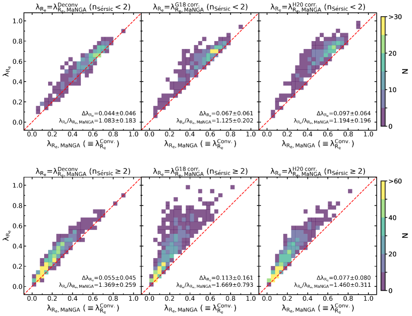
Figure 13: (Top panels) Each panel shows comparison between the $\lambda_{R_{e}}$ measured from the original MaNGA IFU data and the $\lambda_{R_{e}}$ measured from the deconvolved MaNGA IFU data (left), the $\lambda_{R_{e}}$ corrected by following G18 (center), and the $\lambda_{R_{e}}$ corrected by following H20 (right), using the MaNGA galaxies with $n_{S\acute{e}rsic}<2$. Distribution of points are shown as 2D histogram. (Bottom panels) Same as the top panels but using the MaNGA galaxies with $n_{S\acute{e}rsic}\geq 2$.

5.2 Application to MaNGA Data

We measure $\lambda_{R_{e}}$ by using both the original and the PSF-deconvolved MaNGA data, and investigate the difference in the measured $\lambda_{R_{e}}$ values that is induced by the deconvolution. We use 2D velocity and the velocity dispersion distribution (subsection 4.2) along with the reconstructed MaNGA $r$-band flux data of 4,426 MaNGA galaxies that we measured in section 4. We use ’NSA_ELPETRO_TH50_R’, ’NSA_ELPETRO_BA’, ’NSA_ELPETRO_PHI’, ’IFURA/IFUDEC’ and ’OBJRA/OBJDEC’ in the FITS header of each galaxy IFU data to evaluate the concentric ellipse of each. To ensure the quality of measured $\lambda_{R_{e}}$, we did not include certain spaxels in the $\lambda_{R_{e}}$ calculation when a spaxel has 1) median $\rm{S/N}_{pPXF}<10$, or 2) velocity dispersion $<$ 40 km/s, following the prescription of Lee et al. (2018). We also did not include spaxels with spurious kinematics to the $\lambda_{R_{e}}$ calculation, where the absolute value of velocity is greater than 500 km/s or the velocity dispersion is less than 50 km/s. When the number fraction of the excluded spaxels within 1${\rm{R}_{e}}$ becomes larger than 30%, we do not use the $\lambda_{R_{e}}$ from that galaxy for the further analysis. Although we use the same elliptical aperture for the measurement of both $\rm\lambda_{R_{e},MaNGA}$ and $\rm\lambda_{R_{e},MaNGA,Deconv.}$, the number of spaxels used for each measurement is not always identical because of $\rm{S/N}_{pPXF}$ and velocity dispersion criteria. We also exclude the galaxies flagged with ’CRITICAL’ by the MaNGA Data Reduction Pipeline or Data Analysis Pipeline (Law et al., 2016; Westfall et al., 2019). These criteria would be sufficient to observe the impact of deconvolution on $\lambda_{R_{e}}$ for the real data. We note that more strict quality control criteria should be applied for the further analysis using $\lambda_{R_{e}}$ (Lee et al., 2018; Graham et al., 2018). The number of galaxies having both quality assured $\rm\lambda_{R_{e},MaNGA}$ and $\rm\lambda_{R_{e},MaNGA,Deconv.}$ is 2,268. We present the relation between the $\rm\lambda_{R_{e},MaNGA}$ and the $\rm\lambda_{R_{e},MaNGA,Deconv.}$ in the left most panels of Figure 13 depending on $n_{S\acute{e}rsic}$ of the MaNGA galaxies (NSA_SERSIC_N). Compare to the $\rm\lambda_{R_{e},MaNGA}$, most of the $\rm\lambda_{R_{e},MaNGA,Deconv.}$ values are moderately increased for both $n_{S\acute{e}rsic}$ ranges. The median and standard deviation of $\rm\Delta\lambda_{R_{e}}$ is $\rm 0.044\pm 0.046$, or median increase of 8 percent with 18 percent point standard deviation for galaxies with $n_{S\acute{e}rsic}<2$. The median and standard deviation of $\rm\Delta\lambda_{R_{e}}$ is $\rm 0.055\pm 0.045$, or median increase of 37 percent with 26 percent point standard deviation for galaxies with $n_{S\acute{e}rsic}\geq 2$. Note that the fractional difference is larger for the galaxies with $n_{S\acute{e}rsic}\geq 2$ because the majority of $n_{S\acute{e}rsic}\geq 2$ galaxies have relatively small $\rm\lambda_{R_{e}}$ values compared to $n_{S\acute{e}rsic}<2$ galaxies. We also check the correlation between the two ratios ($\rm\lambda_{R_{e},MaNGA}/\lambda_{R_{e},MaNGA,Deconv.}$ and $\rm FWHM_{PSF}/R_{e}$) and as expected from the result with mock IFU data, $\rm\lambda_{R_{e},MaNGA,Deconv.}/\lambda_{R_{e},MaNGA}$ increases as $\rm FWHM_{PSF}/R_{e}$ increases.

During the validity check of the calculated $\rm\lambda_{R_{e}}$, we find tens or more of galaxies that their $\lambda_{R_{e}}$ do not seem measured correctly. There are several such cases, for example,

1. There are seven galaxies in Figure 13 that have both $\rm\lambda_{R_{e},MaNGA}$ and $\rm\lambda_{R_{e},MaNGA,Deconv.}>$ 0.8. However, all of those galaxies’ systematic velocity are highly underestimated or overestimated, in other words, galaxy systematic velocity derived by the NSA redshift is not matching with the true systematic velocity. After correcting its systematic velocity, it turns out their $\lambda_{R_{e}}$ value is significantly less than 0.8.

2. There are galaxies with foreground/background objects, either star or other galaxies, at or around the $\rm 1{\rm{R}_{e}}$ elliptical aperture. Some of them are already masked by MaNGA data reduction pipeline, but still there are tens of IFU data with unmasked interloper. Either masked or unmasked, the interloping object disrupt the kinematics measurement in particular at the border between the object of interest and the interloper.

3. Contrary to the sample definition of MaNGA galaxies, there are galaxies where their ${\rm{R}_{e}}$ size is comparable to the IFU field of view. This brings spaxels at the edge of the IFU field of view to the $\lambda_{R_{e}}$ calculation. Since the kinematics measured at near the edge of the deconvolved IFU data could be different from the correct value, the calculated $\lambda_{R_{e}}$ from such galaxy sample is not reliable.

4. IFU data with small field of view (i.e. 12$\arcsec$) often includes only a tens of spaxels to $\lambda_{R_{e}}$ calculation. This means that even a small offset at its center position or systematic velocity can leads considerable change in the measured $\lambda_{R_{e}}$ value. These suggest that more careful data quality assurance is required to assure the data with correctly measured $\lambda_{R_{e}}$ value.

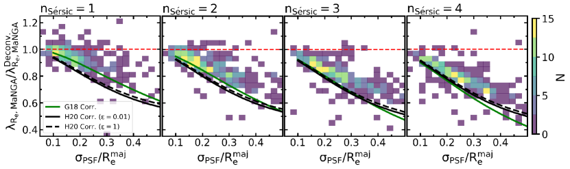
Figure 14: The ratios between the $\lambda_{R_{e}}$ measured from the original MaNGA data and the $\lambda_{R_{e}}$ measured from PSF-deconvolved MaNGA data, depending on $\rm\sigma_{PSF}/R_{e}^{maj.}$. Each panel shows the 2D histogram of $\rm\lambda_{R_{e},MaNGA}/\lambda_{R_{e},MaNGA}^{Deconv.}$ versus $\rm\sigma_{PSF}/R_{e}^{maj.}$, when $n_{S\acute{e}rsic}=$1,2,3, and 4. The overlapped lines show the inverse of G18 and H20 correction functions, which are equal to $\rm\lambda_{R_{e},MaNGA}/\lambda_{R_{e},MaNGA}^{G18\;Corr.}$ (green solid line) or $\rm\lambda_{R_{e},MaNGA}$/$\rm\lambda_{R_{e},MaNGA}^{H20\;Corr.}$ (black lines). Two inverse H20 functions are shown, one when $\rm\epsilon=$0.01 (black solid line) and the other when $\rm\epsilon=$1 (black dashed line).

We also plot the relation between the $\rm\lambda_{R_{e},MaNGA}$ and the corrected $\lambda_{R_{e}}$ (following G18 and H20) in Figure 13. Compared to $\Delta\lambda_{R_{e}}$ caused by the deconvolution method, the $\Delta\lambda_{R_{e}}$ caused by G18 correction is higher. Sometimes the corrected value becomes higher than $\lambda_{R_{e}}=1$ which is nonphysical. As noticed in subsection 5.1, the over-correction could be due to different shape of velocity dispersion profile of real galaxy compare to the profile used to derived the correction function, or some other unanticipated model-dependent bias.

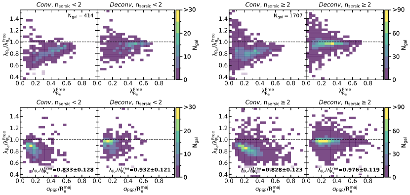
Figure 15: Comparison between the ratios between $\lambda_{R_{e}}$ measured from PSF-Convolved or PSF-Deconvolved IFU data with respect to $\lambda_{R_{e}}^{Free}$ and $\rm\sigma_{PSF}/R_{e}^{maj.}$ using MaNGA DR15 galaxies as the PSF-Free data. Panels on left show $\lambda_{R_{e}}^{Conv}/\lambda_{R_{e}}^{Free}$ and $\lambda_{R_{e}}^{Deconv}/\lambda_{R_{e}}^{Free}$ as a function of $\lambda_{R_{e}}^{Free}$ or $\rm\sigma_{PSF}/R_{e}^{maj.}$ for the original MaNGA galaxies with $n_{S\acute{e}rsic}<2$. Panels on right show the same as the left but using the original MaNGA galaxies with $n_{S\acute{e}rsic}\geq 2$. The median and standard deviation of $\lambda_{R_{e}}/\lambda_{R_{e}}^{Free}$ are noted in bottom panels.

6 Summary and Conclusion

Appendix A Mock IFU Data Generation

In order to quantitatively examine the change made by the deconvolution, the mock IFU data should be generated correctly as per the model galaxy parameters. Here we describe the generation process of each type of mock IFU data (Free, Conv, Deconv) in detail. Initially, an ideal IFU data (Free, without any seeing effect) is produced for each set of galaxy model parameters. Then the PSF-convolved IFU data (Conv) is made by the convolution of a wavelength dependent PSF on the 2D image at each wavelength slice with addition of Gaussian random noise. Deconv IFU data is produced from Conv IFU data by applying the deconvolution method.

An arbitrary synthetic spectrum, composed by single-stellar populations with three different age (1 Gyr (15%), 5 Gyr (60%), 10 Gyr (25%)) from MILES stellar library (Sánchez-Blázquez et al., 2006; Falcón-Barroso et al., 2011; Vazdekis et al., 2010) is chosen as a rest-frame model spectrum (using unimodal initial mass function (Vazdekis et al., 1996) and Padova+00 isochrones (Girardi et al., 2000); $\Delta\lambda=2.51$ Å, $\lambda$ range from 3,540 to 7,410Å)

For each set of galaxy model parameters (subsection 3.2), we generate the Free and Conv mock IFU data, according to the below steps.

1. The spatial and spectral sampling size of the mock IFU data is determined. Following the sampling size and the data structure of MaNGA IFU data, we choose spatial sampling size as 0.5$\arcsec$, and in spectral direction we use a logarithmic wavelength sampling from $\rm log_{10}\lambda=$ 3.5589 to 4.0151, with total number of 4,563 wavelength bins.

2. 2D maps of flux (Sérsic profile), line-of-sight velocity with respect to the galaxy center (Equation 2), velocity dispersion (Equation 3), and S/N distribution (set by S/N at 1 effective radius) are identified as per a set of galaxy model parameters. Angular size of ${\rm{R}_{e}}$ is determined by two parameters, IFU field of view and IFU radial coverage in ${\rm{R}_{e}}$, by dividing half of the IFU field of view by the IFU radial coverage in ${\rm{R}_{e}}$. We assume that all three maps follow the identical geometry as defined by the inclination angle, position angle, $x_{cent}$ and $y_{cent}$. In case of S/N map, a relative S/N map is generated as per the Sersic profile then scaled to have a S/N at 1 ${\rm{R}_{e}}$ as per the galaxy model parameter.

3. At each 2D pixel (Spaxel), a rest-frame spectrum is shifted and broadened in the spectral direction as per the respective line-of-sight velocity and the velocity dispersion value in the 2D map. First, the spectrum is convolved by a Gaussian function as per the velocity dispersion value. Second, the spectrum is redshifted by $z$ of a model galaxy. Third, a spectrum at each spaxel is blue- or red-shifted according to the corresponding line-of-sight velocity value with respect to the galaxy center.

4. (Conv IFU data only) A 2D Gaussian PSF is convolved to the 2D image slice at each wavelength bin. The size of the Gaussian PSF FWHM is determined according to the model FWHM coefficient parameters. For example, in case of $c_{0}=2.6\arcsec$ and $c_{1}=-1.2\times 10^{-5}\arcsec/$Å, $\rm{FWHM}_{\rm{Conv}}$ at $g$-band effective wavelength (4770 Å) is $2.52\arcsec$ (which is median $g$-band PSF FWHM size of the MaNGA galaxies (Figure 8)).

5. A constant spectral resolution (2.9 Å) is applied at each spaxel as a proxy of instrument resolution of the real IFU data. It is done by the convolution of Gaussian function (FWHM=1.45 Å) to each spectrum. The FWHM size of applied Gaussian function is determined by quadratic difference between the instrument spectral resolution and the intrinsic resolution of the model synthetic spectrum (2.51 Å).

6. Noise spectrum at each spaxel is calculated. First, a relative S/N spectrum is calculated from the flux spectrum (assuming Poisson noise), and the relative S/N spectrum is scaled so that the S/N value of the median flux value would be matched to the S/N value in the 2D S/N map (generated in step 2). The noise spectrum is calculated by dividing the flux spectrum by the scaled S/N spectrum. The noise spectrum is not added to the flux spectrum at this stage.

7. Hexagonal shape mask is applied to the IFU data to resemble the MaNGA-like IFU data.

8. (Conv IFU data only) Gaussian random noise is applied to the IFU data using noise spectrum from the step 6. At each spaxel, the noise spectrum is multiplied by the Gaussian random value (-3 to 3) and then added to the flux spectrum.

9. Generated mock spectra are saved in 3D cube FITS format. Each noise spectrum is converted to an inverse variance spectrum (=1/noise²) before saved. Flux, inverse variance, mask, wavelength, and spectral resolution data are saved in FITS extension similar to the actual MaNGA IFU data.

Appendix B Validity of Rotation Curve Model Fitting

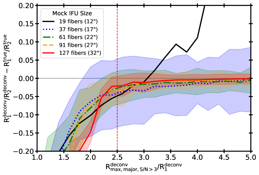
Figure B.1: The difference between the true and fitted RC outer radius slope ($\rm R_{1}/R_{2}$) from the deconvolved mock IFU cubes with respect to the R-ratio ($\rm R_{max,S/N>3,major}/R_{1}$). Color represents the size of mock IFU. Each line represents the median of the normalized RC outer radius slope differences at each bin. Shaded region shows 1-$\sigma$ range of the differences. 1-$\sigma$ range of the 19-fiber size IFU is not shown because it is significantly higher than others. The vertical red-dashed line indicates our choice of R-ratio criteria, which is R-ratio $\rm>2.5$.

In subsection 3.3, we notice that there are cases where the RC model fitting could give an unreliable result under certain circumstances. One case is where the 2D velocity data does not have sufficient radial coverage to constrain the RC slope at the outer radius. For example, in Figure 1, the model would not be able to constrain the RC outer radius slope if the data covers only up to r = 4$\arcsec$. The other case is where the geometry of the fitted galaxy is close to both edge or face-on. In this case, both fitted RC velocity amplitude ($\rm{V}_{ROT}$) and inclination angle ($i$) becomes unreliable. We investigate this two cases in details using use the Group 3 mock IFU data (subsection 3.2) which represents various combinations of galaxy parameters that mimic the actual IFU data. From the result, we estimate the criteria that the result of RC model fitting can be considered as valid.

First, we calculate R-ratio, a ratio between the maximum radial distance along the major axis to the $R_{1}$ parameter value (=$\rm R_{major,S/N>3}/R_{1}$). We define the maximum radial distance as the farthest radial distance among the radial distances of the spaxels which are located within the $\rm\pm 5\arcdeg$ from the major axis and satisfying $\rm S/N_{pPXF}>3$. $\rm S/N_{pPXF}$ is the median $\rm S/N$ of the spectrum that are used for line-of-sight velocity distribution fitting (pPXF routine). Then we plot the relation between the R-ratio and the fitting accuracy of the normalized RC outer slope value as in Figure B.1. Although there are multiple factor which affecting R-ratio including the size of IFU, S/N cut, and Sérsic index, we divide the result depend on its IFU size only because the size causes the most significant systematic difference to the 1-$\sigma$ variation of the normalized RC outer slope accuracy. In Figure B.1, the accuracy of the normalized RC outer radius slope ($\rm{{R}_{1}/{R}_{2}}$) shows strong dependence to the r-ratio. Regardless of the IFU size, the median difference between the true and the fitted $\rm{{R}_{1}/{R}_{2}}$ is large at low R-ratio, and the difference becomes smaller at higher R-ratio, except for the 19-fiber size IFU which is the smallest in its size. The 1-$\sigma$ variation of the $\rm{{R}_{1}/{R}_{2}}$ difference becomes smaller as the mock IFU size increases, mainly because the larger IFU have more spaxels so naturally it can better constraint the parameter values. We didn’t plot the 1-$\sigma$ range of the 19-fiber size IFU because the range is larger than the height of the plot. From the result, we set a criteria of R-ratio $>$ 2.5, to determine whether the measured $\rm{{R}_{1}/{R}_{2}}$ can be considered as valid. Because the difference between the true and the fitted $\rm{{R}_{1}/{R}_{2}}$ becomes stable and small at R-ratio $>$ 2.5 compare to the difference at R-ratio $<$ 2.5 We also find that the $\rm{{R}_{1}/{R}_{2}}$ value measured from 19-fiber size IFU (Field of view equal to 12$\arcsec$) should not be used. This is because the measured $\rm{{R}_{1}/{R}_{2}}$ value remains inaccurate even at R-ratio $>$ 2.5.

We also analyze the relation between the R-ratio and the fitting accuracy of the galaxy kinematic inclination angle in Figure B.2. This result is plotted with the IFU data which are satisfying a criteria of R-ratio $>$ 2.5 only. The result shows that the fitted RC velocity amplitude ($\rm{V}_{ROT}$) is highly uncertain when the fitted inclination angle is low. In addition, 1-$\sigma$ of the median $\rm{V}_{ROT}$ also decreases when the fitted inclination value gets higher. Again we notice that the result of 19-fiber size IFU is not reliable due to its small number of spaxels. There is a slight hint that the fitted result may not be reliable at the higher inclination side, because the 1-$\sigma$ range is getting increased when the inclination angle is high. It can be explained by the low number of total spaxel elements when the inclination angle is high. From the shape of the curves and the 1-$\sigma$ range, we set a conservative criteria of $\rm 25\arcdeg<i^{deconv}<75\arcdeg$ and consider the fitted $\rm{V}_{ROT}$ value as valid when the result meets those criteria.

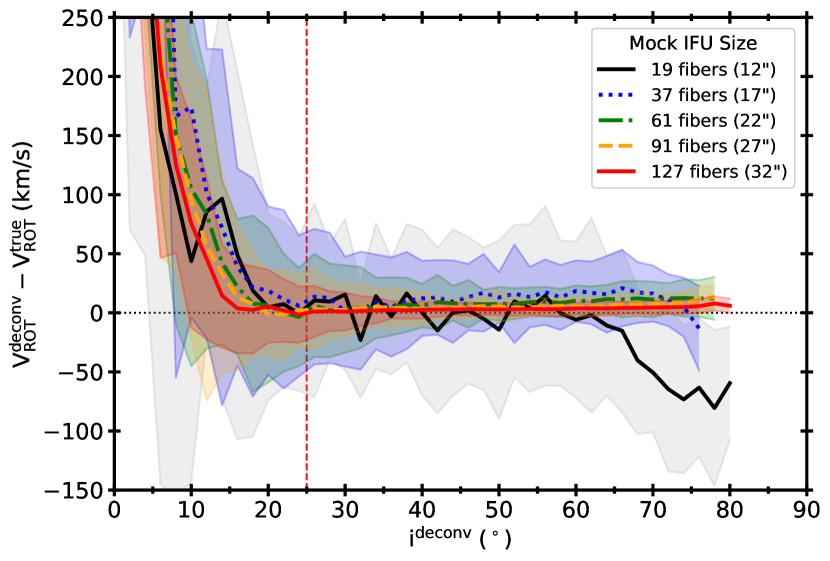
Figure B.2: The difference between the true and fitted RC velocity amplitude ($\rm V_{ROT}$) from the deconvolved mock IFU cubes with respect to the fitted inclination angle. Color represents the size of mock IFU. Solid line represents the median of the RC velocity amplitude differences at each bin. Shaded region shows 1-$\sigma$ range of the differences. The vertical red-dashed line indicates the lower end of our inclination angle criteria choice ($\rm 25\arcdeg<i^{deconv}<75\arcdeg$).

Appendix C Deconvolution Effect Examples

In Figure 2, we presented the example of the effects of PSF convolution and deconvolution to the IFU data. Here we show more examples from our mock IFU data to illustrate the effects of the deconvolution in various mock galaxy parameter space. Examples are taken from Group 1 mock IFU data. Figure C.1 and Figure C.2 show the result of the deconvolution at low S/N ($\rm{S/N}$@1${\rm{R}_{e}}$ = 10) when $n_{S\acute{e}rsic}$ = 1 and 4, $R_{1}$ = 3$\arcsec$, $i$ = 55$\arcdeg$. Figure C.3, Figure C.4, Figure C.5, and Figure C.6 show the result of the deconvolution at different combinations of $i$ (55, 70$\arcdeg$) and $n_{S\acute{e}rsic}$ (1,4), when $\rm{S/N}$ at 1 ${\rm{R}_{e}}$ = 20 and $R_{1}$ = 3$\arcsec$. The forth columns of the all figures represent the significant difference between the maps from Free and Conv. The effect of PSF convolution is crucial in the distribution of Flux, velocity and the velocity dispersion. The fifth columns of the all figures show that the changes made by the PSF convolution are significantly restored by the deconvolution method. However, the restoration is not very effective at the outer radius where S/N becomes low, and also the flux distribution shows non-negligible artifacts around the center of galaxies, in particular when $n_{S\acute{e}rsic}$ = 4. Nevertheless, the velocity and the velocity dispersion are generally well recovered even when the $n_{S\acute{e}rsic}$ = 4.

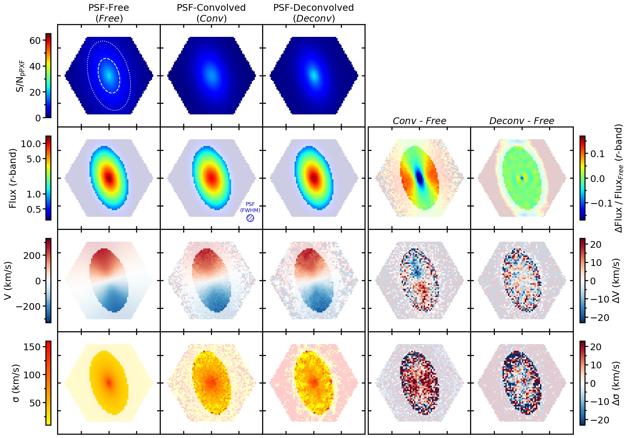
Figure C.1: Plots similar to Figure 2 but for $n_{S\acute{e}rsic}$=1, $R_{1}=3\arcsec$, $1/R_{2}=0.05/\arcsec$, $i=55\arcdeg$, and $\rm{S/N}$@1${\rm{R}_{e}}$ = 10

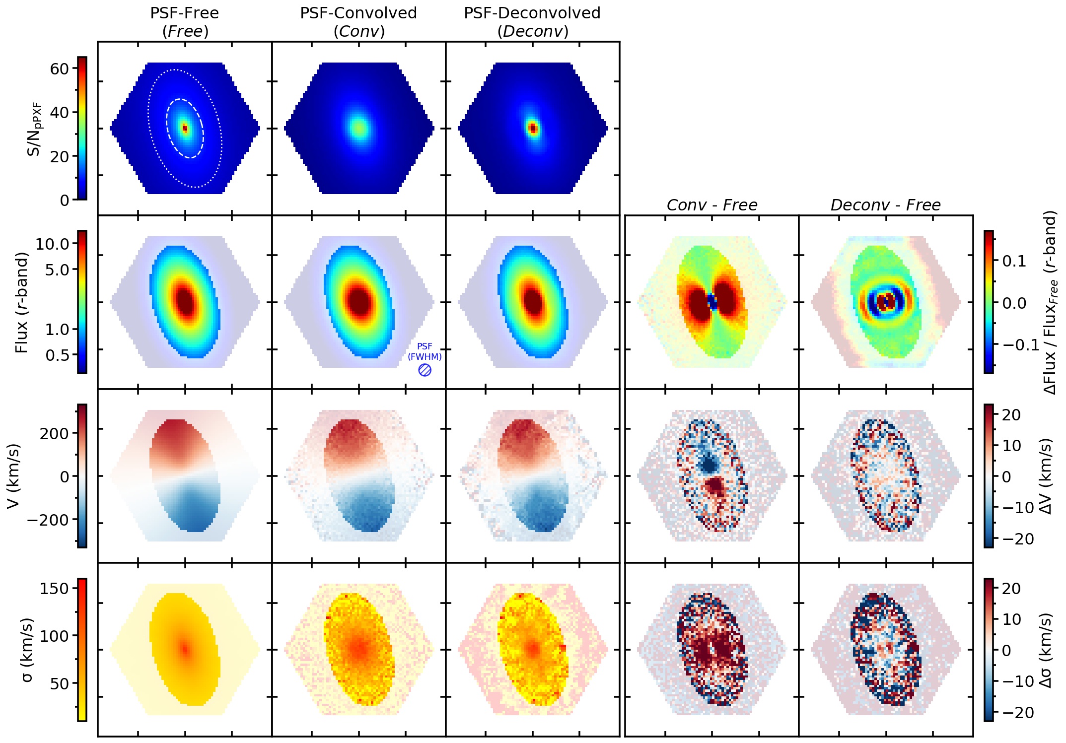
Figure C.2: Plots similar to Figure 2 but for $\rm n_{S\acute{e}rsic}$=4, $R_{1}=3\arcsec$, $1/R_{2}=0.05/\arcsec$, $i=55\arcdeg$, and $\rm{S/N}$@1${\rm{R}_{e}}$ = 10

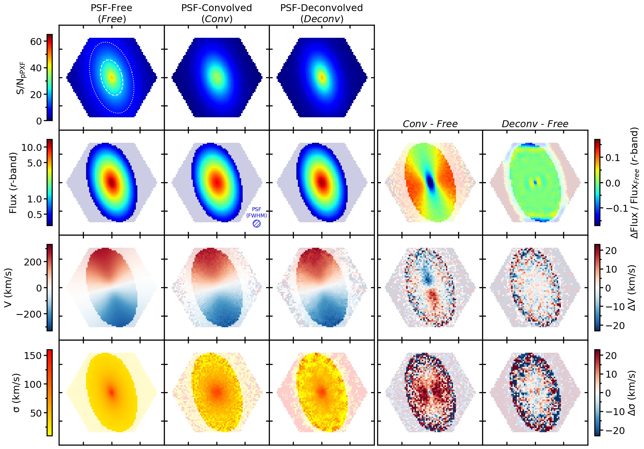
Figure C.3: Plots similar to Figure 2 but for $\rm n_{S\acute{e}rsic}$=1, $R_{1}=3\arcsec$, $1/R_{2}=0.05/\arcsec$, $i=55\arcdeg$, and $\rm{S/N}$@1${\rm{R}_{e}}$ = 20

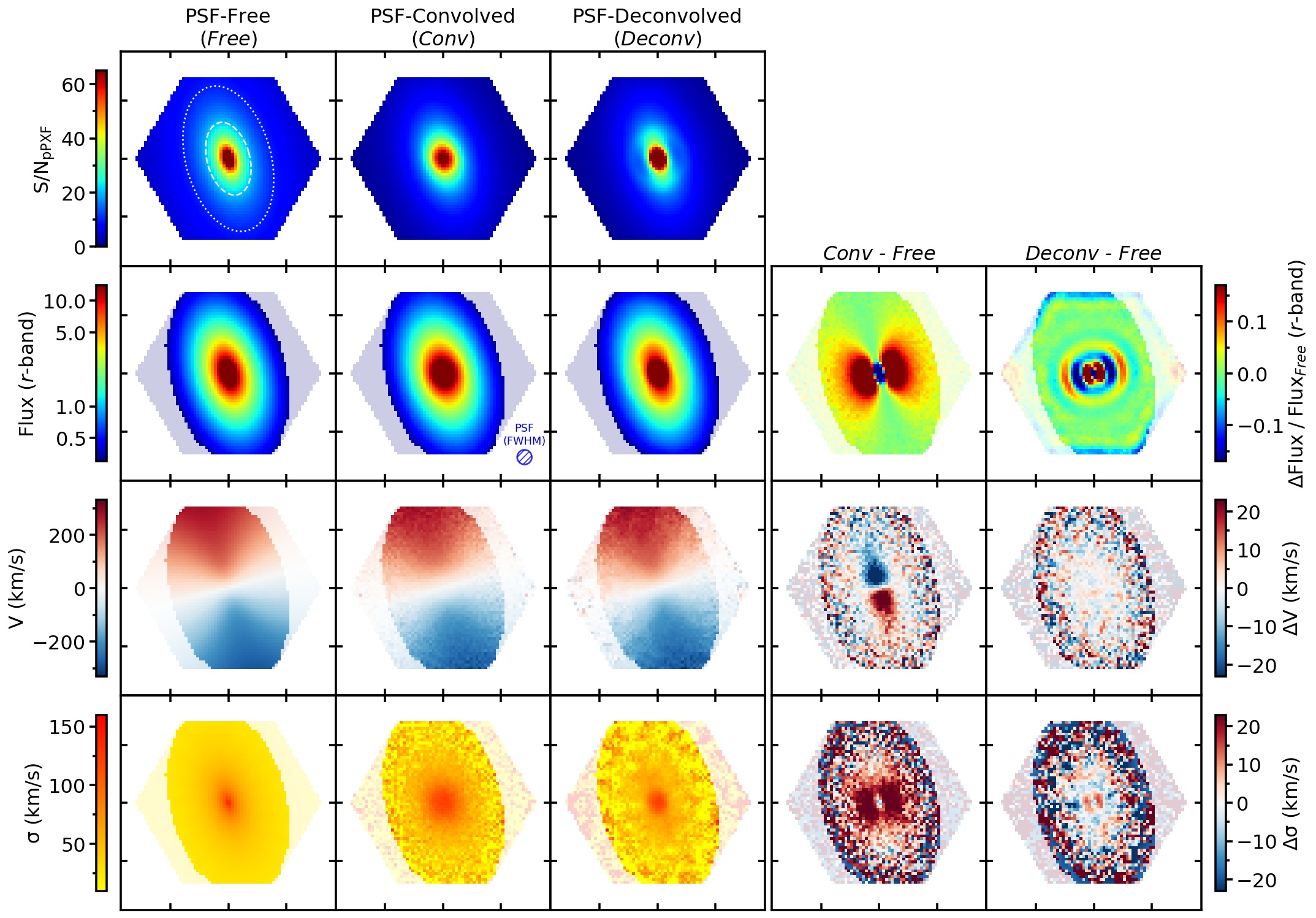
Figure C.4: Plots similar to Figure 2 but for $\rm n_{S\acute{e}rsic}$=4, $R_{1}=3\arcsec$, $1/R_{2}=0.05/\arcsec$, $i=55\arcdeg$, and $\rm{S/N}$@1${\rm{R}_{e}}$ = 20

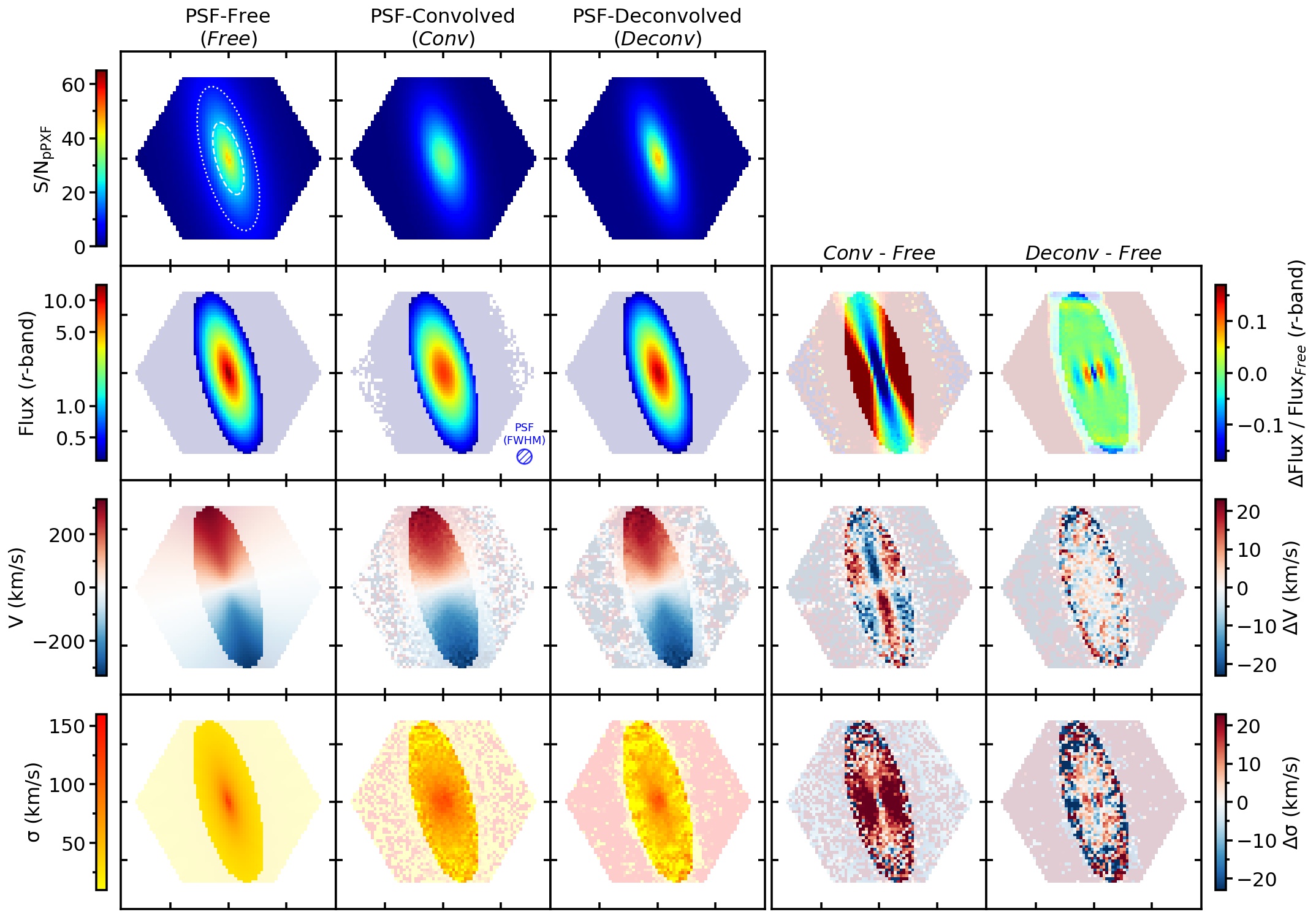
Figure C.5: Plots similar to Figure 2 but for $\rm n_{S\acute{e}rsic}$=1, $R_{1}=3\arcsec$, $1/R_{2}=0.05/\arcsec$, $i=70\arcdeg$, and $\rm{S/N}$@1${\rm{R}_{e}}$ = 20

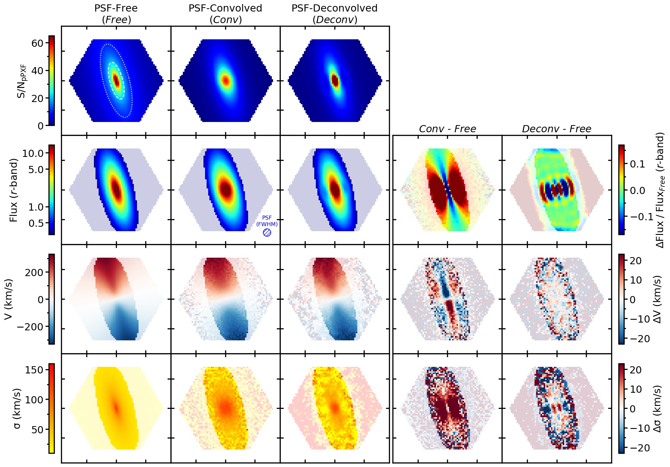
Figure C.6: Plots similar to Figure 2 but for $\rm n_{S\acute{e}rsic}$=4, $R_{1}=3\arcsec$, $1/R_{2}=0.05/\arcsec$, $i=70\arcdeg$, and $\rm{S/N}$@1${\rm{R}_{e}}$ = 20

Appendix D Dependence on Deconvolution Parameters

D.1 Number of Deconvolution Iterations

In section 3.4.2, we described the relationship between $\rm{N}_{iter}$ and the restored model kinematic parameters (Figure 4). Here we give similar plots with model galaxies of different parameters to provide more insight into the determination of $\rm{N}_{iter}$ to the readers. Figure D.2, Figure D.3, Figure D.4, Figure D.5 are complementary figures to the Figure 4. The figures show the relations between the fitted RC model parameter and the $\rm{N}_{iter}$ for different $R_{1}$ (2, 3, 4 ($\arcsec$)) and $1/R_{2}$ (-0.05, 0, 0.05 ($1/\arcsec$)). The result is consistent with Figure 4 thus the $\rm{N}_{iter}$ = 20 is an adequate choice for the deconvolution.

D.2 Size of PSF FWHM

Here we show the relation between $\rm{FWHM_{Deconv}}$ and the restored model kinematic parameters. We present plots similar to the Figure 5 but with different model galaxies as well as different $\rm{FWHM_{Conv}}$.

Figure D.6, Figure D.7, Figure D.8, and Figure D.9 are complementary figures to the Figure 5. The figures show the relation between the fitted RC model parameter and the $\rm{FWHM}_{\rm{Deconv}}$ with different $R_{1}$ (2, 3, 4 ($\arcsec$)) and $1/R_{2}$ (-0.05, 0, 0.05 ($1/\arcsec$)). The result is consistent with Figure 5 thus the result of the deconvolution is consistent when $|\rm{FWHM}_{\rm{Deconv}}-\rm{FWHM}_{\rm{Conv}}|$ is smaller then the $\rm{FWHM}_{\rm{PSF}}$ measurement error (0.2$\arcsec$).

Figure D.10 and Figure D.11 show the result of the deconvolution with different $\rm{FWHM}_{\rm{Conv}}$ (2.3, 2.9 ($\arcsec$)). Again, the result of the deconvolution is consistent when $|\rm{FWHM}_{\rm{Deconv}}-\rm{FWHM}_{\rm{Conv}}|$ is small.

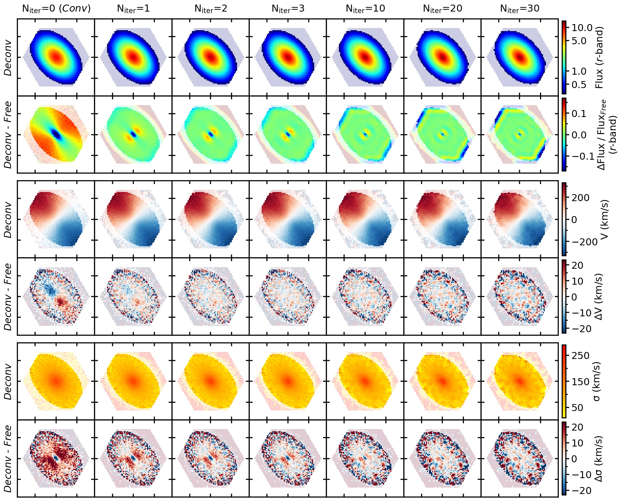
Figure D.1: Effect of the number of deconvolution iterations ($\rm{N}_{iter}$) to the 2D maps of $r$-band flux, line of sight velocity (V) and velocity dispersion ($\sigma$). The first and second rows show 2D flux map from the deconvolved mock IFU data and the difference between the 2D flux map from the deconvolved mock IFU data and the PSF-free mock IFU data at selected $\rm{N}_{iter}$ = 0, 1, 2, 3, 10, 20, 30, respectively. The third and fourth rows show the same for the 2D line of sight velocity map, and the fifth and sixth rows show the same for the 2D velocity dispersion map. The 2D maps for $\rm{N}_{iter}$=0 and $\rm{N}_{iter}$=20 are the same as in the Figure 2.

Figure D.2: Relations between the RC model parameters and $\rm{N}_{iter}$ for $\rm R_{1}=3,1/R_{2}=-0.05$

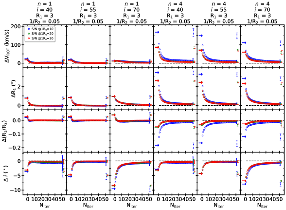
Figure D.3: Plots similar to Figure D.2 but for $\rm R_{1}=3,1/R_{2}=0$

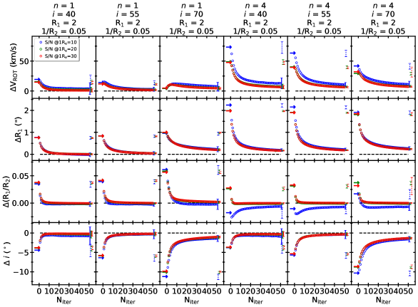
Figure D.4: Plots similar to Figure D.2 but for $\rm R_{1}=2,1/R_{2}=0.05$

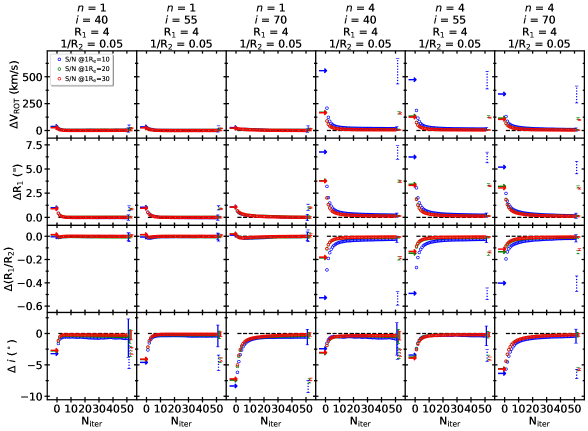
Figure D.5: Plots similar to Figure D.2 but for $\rm R_{1}=4,1/R_{2}=0.05$

Figure D.6: Relations between the RC model parameters and $\rm{FWHM}_{\rm{Deconv}}$ for $\rm R_{1}=3,1/R_{2}=-0.05,FWHMc_{0}=2.6$

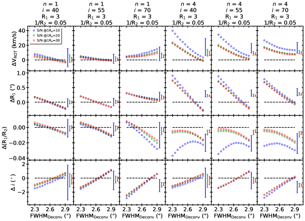
Figure D.7: Plots similar to Figure D.6 but for $\rm R_{1}=3,1/R_{2}=0.05,FWHMc_{0}=2.6$

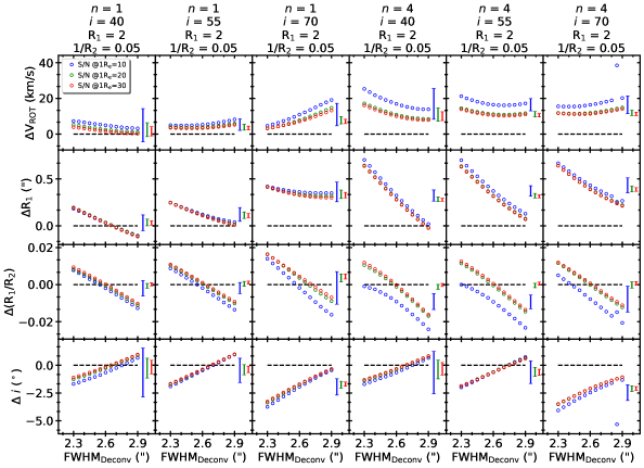
Figure D.8: Plots similar to Figure D.6 but for $\rm R_{1}=2,1/R_{2}=0.05,FWHMc_{0}=2.6$

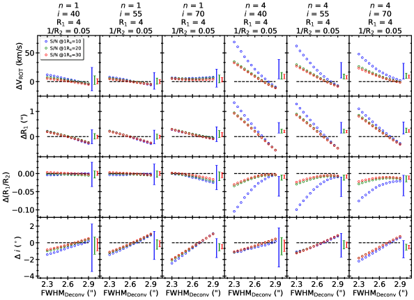
Figure D.9: Plots similar to Figure D.6 but for $\rm R_{1}=4,1/R_{2}=0.05,FWHMc_{0}=2.6$

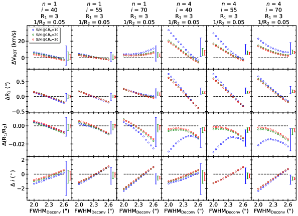
Figure D.10: Plots similar to Figure D.6 but for $\rm R_{1}=3,1/R_{2}=0.05,FWHMc_{0}=2.3$

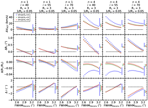
Figure D.11: Plots similar to Figure D.6 but for $\rm R_{1}=3,1/R_{2}=0.05,FWHMc_{0}=2.9$

Appendix E Effect of PSF Convolution to the Spin Parameter Measurement

In Figure E.1, we plot the relations between the $\lambda_{R_{e}}$ ratios ($\lambda_{R_{e}}^{Conv}/\lambda_{R_{e}}^{Free}$, $\lambda_{R_{e}}^{Deconv}/\lambda_{R_{e}}^{Free}$, $\lambda_{R_{e}}^{G18Corr.}/\lambda_{R_{e}}^{Free}$) and the true $\lambda_{R_{e}}$ value ($\lambda_{R_{e}}^{Free}$), depends on three mock IFU parameters, IFU field of view, $n_{S\acute{e}rsic}$, and IFU radial coverage in ${\rm{R}_{e}}$, using Group 3 mock IFU data (subsection 3.1). Most of the panel of Figure E.1 shows that $\lambda_{R_{e}}$ ratios have little or negligible dependence on $\lambda_{R_{e}}^{Free}$, except when $\lambda_{R_{e}}^{Free}$ $<$ 0.1. The ratio and its standard deviation at $\lambda_{R_{e}}^{Free}$ $<$ 0.1 looks different compare to the ratios at $\lambda_{R_{e}}^{Free}$ $>$ 0.1, but this is simply an effect of small denominator when $\lambda_{R_{e}}^{Free}$ $<$ 0.1. Since the denominator ($\lambda_{R_{e}}^{Free}$) is already small, the actual deviation of $\lambda_{R_{e}}$ values to the true value ($\lambda_{R_{e}}-\lambda_{R_{e}}^{Free}$) is also small. The median and the median of standard deviation of each binned relation ($\rm\Delta\lambda_{R_{e}}^{Free}$=0.1) is used to show the overall dependence of the ratios to the mock IFU parameters as in Figure 11. Unlike average value of entire points, use of median of the binned relations could avoid the contribution from large difference and the standard deviation from the points at $\lambda_{R_{e}}^{Free}<$ 0.1. In Figure E.2 We plot the relation between the $\lambda_{R_{e}}$ ratios and the true $\lambda_{R_{e}}$ value, depend on $n_{S\acute{e}rsic}$ and $\sigma^{\prime}$ parameters using the additional set of mock IFU data (subsection 5.1). Again the median and the median of standard deviation of each binned relation ($\rm\Delta\lambda_{R_{e}}^{Free}$=0.1) is used to show the overall dependence of the ratios to the mock IFU parameters as in Figure 12.

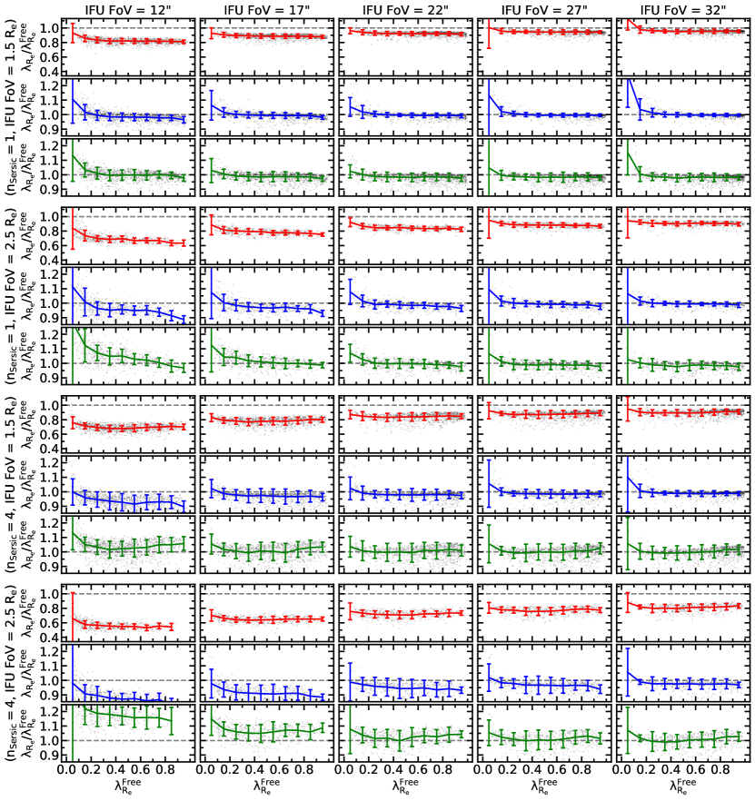
Figure E.1: Relations between the ratio of $\lambda_{R_{e}}$ values ($\lambda_{R_{e}}^{Conv}$, $\lambda_{R_{e}}^{Deconv}$, $\lambda_{R_{e}}^{G18Corr.}$) and the true $\lambda_{R_{e}}$ value ($\lambda_{R_{e}}^{Free}$) as a function of $\lambda_{R_{e}}^{Free}$. Each panel with red, blue, and green lines represents data points with $\lambda_{R_{e}}^{Conv}/\lambda_{R_{e}}^{Free}$, $\lambda_{R_{e}}^{Deconv}/\lambda_{R_{e}}^{Free}$, and $\lambda_{R_{e}}^{G18Corr.}/\lambda_{R_{e}}^{Free}$, respectively. Each column represents the field of view of mock IFU data used for each panel (IFU field of view = 12$\arcsec$, 17$\arcsec$, 22$\arcsec$, 27$\arcsec$, 32$\arcsec$). Each of continuous three rows represent the different combination of $n_{S\acute{e}rsic}$ and the IFU radial coverage in ${\rm{R}_{e}}$ ($n_{S\acute{e}rsic}$=1 & radial coverage of 1.5 ${\rm{R}_{e}}$, $n_{S\acute{e}rsic}$=1 & radial coverage of 2.5 ${\rm{R}_{e}}$, $n_{S\acute{e}rsic}$=4 & radial coverage of 1.5 ${\rm{R}_{e}}$, $n_{S\acute{e}rsic}$=4 & radial coverage of 2.5 ${\rm{R}_{e}}$). Data points are plotted as grey dots in the background. Color lines and the corresponding error bars are the median and the standard deviation of the data points from each bin with the bin size of $\rm\Delta\lambda_{R_{e}}^{Free}$=0.1.

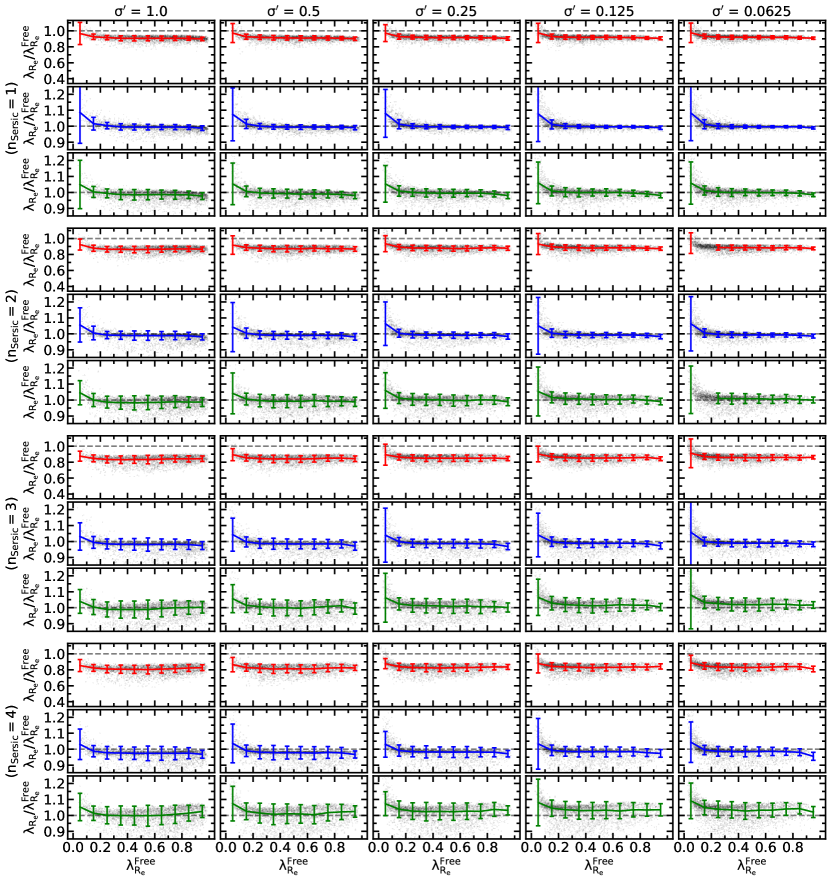
Figure E.2: Relations between the ratio of $\lambda_{R_{e}}$ values ($\lambda_{R_{e}}^{Conv}$, $\lambda_{R_{e}}^{Deconv}$, $\lambda_{R_{e}}^{G18Corr.}$) and the true $\lambda_{R_{e}}$ value ($\lambda_{R_{e}}^{Free}$) as a function of $\lambda_{R_{e}}^{Free}$, similar to Figure E.1 but using different set of mock IFU data (subsection 5.1). Each column represents different velocity dispersion profile steepness of the mock IFU data used for each panel ($\sigma^{\prime}$ = 1, 0.5, 0.25, 0.125, 0.0625). Each of continuous three rows represents different $n_{S\acute{e}rsic}$ of the mock IFU data ($n_{S\acute{e}rsic}$=1,2,3,4). Data points, color lines and the corresponding error bars are plotted in the same way as Figure E.1.

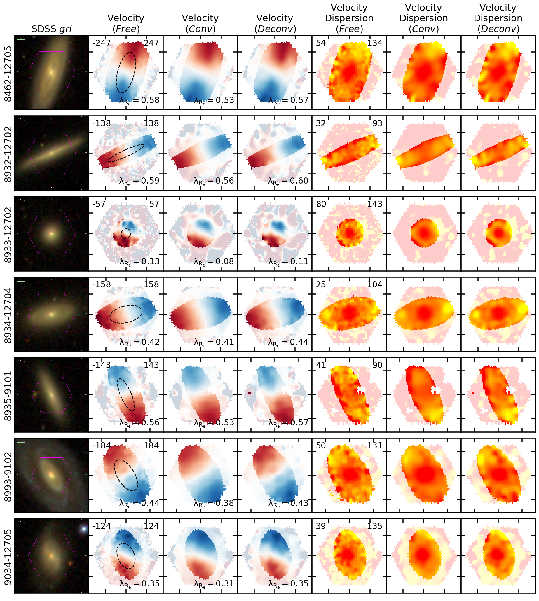
Figure E.3: The velocity and velocity distribution of selected nearby MaNGA galaxies (z$<$0.023 and IFU FoV $\geq$27″). Distributions in Free column are velocity and velocity dispersion distribution measured from the original MaNGA IFU data. Distributions in the other columns (Conv and Deconv) are measured from PSF convolved and deconvolved (PSF FWHM=2.6″) to the original MaNGA IFU data. The ellipses (black-dashed) in the left most column show 1 $\rm R_{e}$ aperture where the $\lambda_{R_{e}}$ values are measured. The values in the top left and top right at each panel in the second and fifth columns indicate the minimum and the maximum range of color, where the color bars are the same as in the Figure 2 (Blue to red for the velocity distribution and yellow to red for the velocity dispersion distribution). Each major tick interval corresponds to 10$\arcsec$.

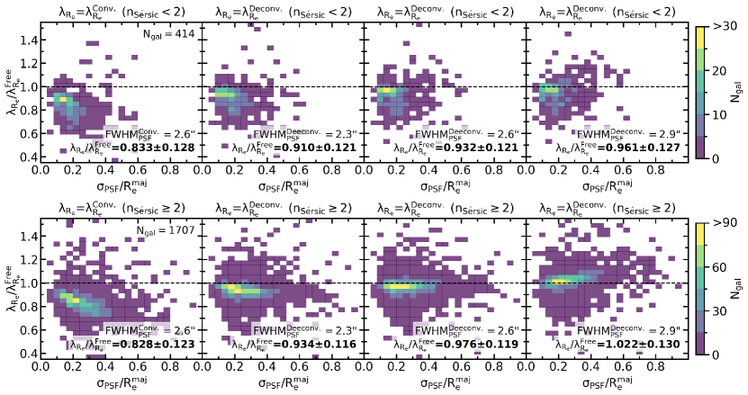
Figure E.4: Comparison between the $\lambda_{R_{e}}$ measured from PSF-Convolved and PSF-Deconvolved IFU data using MaNGA DR15 galaxies as the PSF-Free data, when the $\rm{FWHM}_{\rm{PSF}}$ used for the deconvolution or $\lambda_{R_{e}}$ correction is different from the $\rm{FWHM}_{\rm{PSF}}$ of the convolved PSF. Upper and lower rows show the results when $n_{S\acute{e}rsic}<2$ and $n_{S\acute{e}rsic}\geq 2$, respectively. First column shows $\lambda_{R_{e}}^{Conv}/\lambda_{R_{e}}^{Free}$ as a function of $\rm\sigma_{PSF}/R_{e}^{maj.}$. Second, third, and fourth columns shows $\lambda_{R_{e}}^{Deconv}/\lambda_{R_{e}}^{Free}$ as a function of $\rm\sigma_{PSF}/R_{e}^{maj.}$, but when $\rm{FWHM}_{\rm{PSF}}$ used for the deconvolution or $\lambda_{R_{e}}$ correction is 2.3, 2.6, and 2.9$\arcsec$, respectively. The median and standard deviation of $\Delta\lambda_{R_{e}}$ are noted in each panel.

References

- Aguado et al. (2019) Aguado, D. S., Ahumada, R., Almeida, A., et al. 2019, ApJS, 240, 23, doi: 10.3847/1538-4365/aaf651
- Allington-Smith et al. (2002) Allington-Smith, J., Murray, G., Content, R., et al. 2002, PASP, 114, 892, doi: 10.1086/341712
- Andersen & Bershady (2013) Andersen, D. R., & Bershady, M. A. 2013, ApJ, 768, 41, doi: 10.1088/0004-637X/768/1/41
- Bacon et al. (2001) Bacon, R., Copin, Y., Monnet, G., et al. 2001, MNRAS, 326, 23, doi: 10.1046/j.1365-8711.2001.04612.x
- Bacon et al. (2010) Bacon, R., Accardo, M., Adjali, L., et al. 2010, in Society of Photo-Optical Instrumentation Engineers (SPIE) Conference Series, Vol. 7735, Ground-based and Airborne Instrumentation for Astronomy III, ed. I. S. McLean, S. K. Ramsay, & H. Takami, 773508, doi: 10.1117/12.856027
- Bershady et al. (2010) Bershady, M. A., Verheijen, M. A. W., Swaters, R. A., et al. 2010, ApJ, 716, 198, doi: 10.1088/0004-637X/716/1/198
- Bongard et al. (2011) Bongard, S., Soulez, F., Thiébaut, É., & Pecontal, É. 2011, MNRAS, 418, 258, doi: 10.1111/j.1365-2966.2011.19480.x
- Bouché et al. (2015) Bouché, N., Carfantan, H., Schroetter, I., Michel-Dansac, L., & Contini, T. 2015, AJ, 150, 92, doi: 10.1088/0004-6256/150/3/92
- Bourguignon et al. (2011) Bourguignon, S., Carfantan, H., Slezak, E., & Mary, D. 2011, in 2011 3rd Workshop on Hyperspectral Image and Signal Processing: Evolution in Remote Sensing (WHISPERS), 1–4, doi: 10.1109/WHISPERS.2011.6080853
- Bundy et al. (2015) Bundy, K., Bershady, M. A., Law, D. R., et al. 2015, ApJ, 798, 7, doi: 10.1088/0004-637X/798/1/7
- Cappellari (2002) Cappellari, M. 2002, MNRAS, 333, 400, doi: 10.1046/j.1365-8711.2002.05412.x
- Cappellari (2008) —. 2008, MNRAS, 390, 71, doi: 10.1111/j.1365-2966.2008.13754.x
- Cappellari (2016) —. 2016, ARA&A, 54, 597, doi: 10.1146/annurev-astro-082214-122432
- Cappellari (2017) —. 2017, MNRAS, 466, 798, doi: 10.1093/mnras/stw3020
- Cappellari & Emsellem (2004) Cappellari, M., & Emsellem, E. 2004, PASP, 116, 138, doi: 10.1086/381875
- Cappellari et al. (2013) Cappellari, M., Scott, N., Alatalo, K., et al. 2013, MNRAS, 432, 1709, doi: 10.1093/mnras/stt562
- Choi & Yi (2017) Choi, H., & Yi, S. K. 2017, ApJ, 837, 68, doi: 10.3847/1538-4357/aa5e4b
- Choi et al. (2018) Choi, H., Yi, S. K., Dubois, Y., et al. 2018, ApJ, 856, 114, doi: 10.3847/1538-4357/aab08f
- Chung (2021) Chung, H. 2021, First Release of IFU data deconvolution code, 1.0.0, Zenodo, doi: 10.5281/zenodo.4783185
- Cooley & Tukey (1965) Cooley, J. W., & Tukey, J. W. 1965, Mathematics of computation, 19, 297
- Cortese et al. (2016) Cortese, L., Fogarty, L. M. R., Bekki, K., et al. 2016, MNRAS, 463, 170, doi: 10.1093/mnras/stw1891
- Courbin et al. (2000) Courbin, F., Magain, P., Kirkove, M., & Sohy, S. 2000, ApJ, 529, 1136, doi: 10.1086/308291
- D’Eugenio et al. (2013) D’Eugenio, F., Houghton, R. C. W., Davies, R. L., & Dalla Bontà, E. 2013, MNRAS, 429, 1258, doi: 10.1093/mnras/sts406
- Dressler et al. (2011) Dressler, A., Bigelow, B., Hare, T., et al. 2011, PASP, 123, 288, doi: 10.1086/658908
- Emsellem et al. (1994) Emsellem, E., Monnet, G., & Bacon, R. 1994, A&A, 285, 723
- Emsellem et al. (2007) Emsellem, E., Cappellari, M., Krajnović, D., et al. 2007, MNRAS, 379, 401, doi: 10.1111/j.1365-2966.2007.11752.x
- Emsellem et al. (2011) —. 2011, MNRAS, 414, 888, doi: 10.1111/j.1365-2966.2011.18496.x
- Falcón-Barroso et al. (2011) Falcón-Barroso, J., Sánchez-Blázquez, P., Vazdekis, A., et al. 2011, A&A, 532, A95, doi: 10.1051/0004-6361/201116842
- Feng & Gallo (2011) Feng, J. Q., & Gallo, C. F. 2011, Research in Astronomy and Astrophysics, 11, 1429, doi: 10.1088/1674-4527/11/12/005
- Girardi et al. (2000) Girardi, L., Bressan, A., Bertelli, G., & Chiosi, C. 2000, A&AS, 141, 371, doi: 10.1051/aas:2000126
- Graham et al. (2018) Graham, M. T., Cappellari, M., Li, H., et al. 2018, MNRAS, 477, 4711, doi: 10.1093/mnras/sty504
- Greene et al. (2018) Greene, J. E., Leauthaud, A., Emsellem, E., et al. 2018, ApJ, 852, 36, doi: 10.3847/1538-4357/aa9bde
- Harborne et al. (2020) Harborne, K. E., van de Sande, J., Cortese, L., et al. 2020, MNRAS, 497, 2018, doi: 10.1093/mnras/staa1847
- Henault et al. (2003) Henault, F., Bacon, R., Bonneville, C., et al. 2003, in Society of Photo-Optical Instrumentation Engineers (SPIE) Conference Series, Vol. 4841, Instrument Design and Performance for Optical/Infrared Ground-based Telescopes, ed. M. Iye & A. F. M. Moorwood, 1096–1107, doi: 10.1117/12.462334
- Hopkins et al. (2010) Hopkins, P. F., Bundy, K., Hernquist, L., Wuyts, S., & Cox, T. J. 2010, MNRAS, 401, 1099, doi: 10.1111/j.1365-2966.2009.15699.x
- Jesseit et al. (2009) Jesseit, R., Cappellari, M., Naab, T., Emsellem, E., & Burkert, A. 2009, MNRAS, 397, 1202, doi: 10.1111/j.1365-2966.2009.14984.x
- Kelz et al. (2006) Kelz, A., Verheijen, M. A. W., Roth, M. M., et al. 2006, PASP, 118, 129, doi: 10.1086/497455
- Lagos et al. (2017) Lagos, C. d. P., Theuns, T., Stevens, A. R. H., et al. 2017, MNRAS, 464, 3850, doi: 10.1093/mnras/stw2610
- Law et al. (2015) Law, D. R., Yan, R., Bershady, M. A., et al. 2015, AJ, 150, 19, doi: 10.1088/0004-6256/150/1/19
- Law et al. (2016) Law, D. R., Cherinka, B., Yan, R., et al. 2016, AJ, 152, 83, doi: 10.3847/0004-6256/152/4/83
- Le Fèvre et al. (2005) Le Fèvre, O., Vettolani, G., Garilli, B., et al. 2005, A&A, 439, 845, doi: 10.1051/0004-6361:20041960
- Lee et al. (2018) Lee, J. C., Hwang, H. S., & Chung, H. 2018, MNRAS, 477, 1567, doi: 10.1093/mnras/sty729
- Lucy (1974) Lucy, L. B. 1974, AJ, 79, 745, doi: 10.1086/111605
- Lucy & Walsh (2003) Lucy, L. B., & Walsh, J. R. 2003, AJ, 125, 2266, doi: 10.1086/368144
- Magain et al. (1998) Magain, P., Courbin, F., & Sohy, S. 1998, ApJ, 494, 472, doi: 10.1086/305187
- Martin et al. (2018) Martin, G., Kaviraj, S., Devriendt, J. E. G., Dubois, Y., & Pichon, C. 2018, MNRAS, 480, 2266, doi: 10.1093/mnras/sty1936
- Naab et al. (2014) Naab, T., Oser, L., Emsellem, E., et al. 2014, MNRAS, 444, 3357, doi: 10.1093/mnras/stt1919
- Penoyre et al. (2017) Penoyre, Z., Moster, B. P., Sijacki, D., & Genel, S. 2017, MNRAS, 468, 3883, doi: 10.1093/mnras/stx762
- Press et al. (2007) Press, W. H., Teukolsky, S. A., Vetterling, W. T., & Flannery, B. P. 2007, Numerical recipes 3rd edition: The art of scientific computing (Cambridge university press)
- Puech et al. (2008) Puech, M., Flores, H., Hammer, F., et al. 2008, A&A, 484, 173, doi: 10.1051/0004-6361:20079313
- Richardson (1972) Richardson, W. H. 1972, Journal of the Optical Society of America (1917-1983), 62, 55
- Rodet et al. (2008) Rodet, T., Orieux, F., Giovannelli, J.-F., & Abergel, A. 2008, IEEE Journal of Selected Topics in Signal Processing, 2, 802, doi: 10.1109/JSTSP.2008.2006392
- Sánchez et al. (2016) Sánchez, S. F., García-Benito, R., Zibetti, S., et al. 2016, A&A, 594, A36, doi: 10.1051/0004-6361/201628661
- Sánchez-Blázquez et al. (2006) Sánchez-Blázquez, P., Peletier, R. F., Jiménez-Vicente, J., et al. 2006, MNRAS, 371, 703, doi: 10.1111/j.1365-2966.2006.10699.x
- Scott et al. (2018) Scott, N., van de Sande, J., Croom, S. M., et al. 2018, MNRAS, 481, 2299, doi: 10.1093/mnras/sty2355
- Sharples et al. (2013) Sharples, R., Bender, R., Agudo Berbel, A., et al. 2013, The Messenger, 151, 21
- Shepp & Vardi (1982) Shepp, L. A., & Vardi, Y. 1982, IEEE Transactions on Medical Imaging, 1, 113, doi: 10.1109/TMI.1982.4307558
- Soulez et al. (2011) Soulez, F., Bongard, S., Thiebaut, E., & Bacon, R. 2011, in 2011 3rd Workshop on Hyperspectral Image and Signal Processing: Evolution in Remote Sensing (WHISPERS), 1–4, doi: 10.1109/WHISPERS.2011.6080865
- van de Sande et al. (2017) van de Sande, J., Bland-Hawthorn, J., Fogarty, L. M. R., et al. 2017, ApJ, 835, 104, doi: 10.3847/1538-4357/835/1/104
- van de Sande et al. (2019) van de Sande, J., Lagos, C. D. P., Welker, C., et al. 2019, MNRAS, 484, 869, doi: 10.1093/mnras/sty3506
- Vazdekis et al. (1996) Vazdekis, A., Casuso, E., Peletier, R. F., & Beckman, J. E. 1996, ApJS, 106, 307, doi: 10.1086/192340
- Vazdekis et al. (2010) Vazdekis, A., Sánchez-Blázquez, P., Falcón-Barroso, J., et al. 2010, MNRAS, 404, 1639, doi: 10.1111/j.1365-2966.2010.16407.x
- Villeneuve & Carfantan (2014) Villeneuve, E., & Carfantan, H. 2014, IEEE Transactions on Image Processing, 23, 4322, doi: 10.1109/TIP.2014.2343461
- Wake et al. (2017) Wake, D. A., Bundy, K., Diamond-Stanic, A. M., et al. 2017, AJ, 154, 86, doi: 10.3847/1538-3881/aa7ecc
- Westfall et al. (2019) Westfall, K. B., Cappellari, M., Bershady, M. A., et al. 2019, AJ, 158, 231, doi: 10.3847/1538-3881/ab44a2
- Yan et al. (2016) Yan, R., Bundy, K., Law, D. R., et al. 2016, AJ, 152, 197, doi: 10.3847/0004-6256/152/6/197