Robust Validation: Confident Predictions
Even When Distributions Shift

Abstract

While the traditional viewpoint in machine learning and statistics assumes training and testing samples come from the same population, practice belies this fiction. One strategy—coming from robust statistics and optimization—is thus to build a model robust to distributional perturbations. In this paper, we take a different approach to describe procedures for robust predictive inference, where a model provides uncertainty estimates on its predictions rather than point predictions. We present a method that produces prediction sets (almost exactly) giving the right coverage level for any test distribution in an $f$-divergence ball around the training population. The method, based on conformal inference, achieves (nearly) valid coverage in finite samples, under only the condition that the training data be exchangeable. An essential component of our methodology is to estimate the amount of expected future data shift and build robustness to it; we develop estimators and prove their consistency for protection and validity of uncertainty estimates under shifts. By experimenting on several large-scale benchmark datasets, including Recht et al.’s CIFAR-v4 and ImageNet-V2 datasets, we provide complementary empirical results that highlight the importance of robust predictive validity.

1 Introduction

The central conceit of statistical machine learning is that data comes from a population, and that a model fit on a training set and validated on a held-out validation set will generalize to future data. Yet this conceit is at best debatable: indeed, Recht, Roelofs, Schmidt, and Shankar [35] create new test sets for the central image recognition CIFAR-10 and ImageNet benchmarks, and they observe that published accuracies drop by between 3–15% on CIFAR and more than 11% on ImageNet (increases in error rate of 50–100%), even though the authors follow the original dataset creation processes. Given this drop in accuracy—even in carefully reproduced experiments—shift in the data generating distribution is inevitable, and should be an essential focus, given the growing applications of machine learning.

To address such distribution shifts and related challenges, a growing literature advocates fitting predictive models that adapt to changes in the data generating distribution. For example, researchers suggest reweighting data to match new test distributions when covariates shift [46, 18], while work on distributional robustness [5, 17, 15, 14, 7, 6, 38] considers fitting models that optimize losses under worst-case distribution changes. Yet the resulting models often are conservative, appear to sacrifice accuracy for robustness, and even more, they may not be robust to natural distribution shifts [47]. The models also come with few tools for validating their performance on new data.

Instead of seeking robust models, we instead advocate focusing on models that provide validity in their predictions: a model should be able to provide some calibrated notion of its confidence, even in the face of distribution shift. Consequently, in this paper we revisit cross validation, validity, and conformal inference [51] from the perspective of robustness, advocating for more robust approaches to cross validation and equipping predictors with valid confidence sets. We present a method for robust predictive inference under distributional shifts, borrowing tools both from conformal inference [51] and distributional robustness. Our method can allow valid inferences even when training and test distributions are distinct, and we provide a (in our view well-motivated, but still heuristic) methodology to estimate plausible amounts of shift to which we should be robust.

To formalize, consider a supervised learning problem of predicting labels $y\in\mathcal{Y}$ from data $x\in\mathcal{X}$, where we assume we have a putative predictive model that outputs scores $s(x,y)$ measuring error (so that $s(x,y)<s(x,y^{\prime})$ means that the model assigns higher likelihood to $y$ than $y^{\prime}$ given $x$). For example, for a probabilistic model $p(y\mid x)$, a typical choice is the negative log likelihood $s(x,y)=-\log(p(y\mid x))$. For a distribution $Q_{0}$ on $\mathcal{X}\times\mathcal{Y}$, we observe $(X_{i},Y_{i})_{i=1}^{n}\stackrel{{\scriptstyle\rm iid}}{{\sim}}Q_{0}$. Future data may come from $Q_{0}$ or a distribution $Q$ near—in some appropriate sense, deriving from distribution shift—to $Q_{0}$, and we wish to output valid predictions for future instances $(X,Y)\sim Q$, where $Q$ is unknown. The goal of this paper is twofold: first, given a level $\alpha\in(0,1)$ and an uncertainty set $\mathcal{Q}$ of plausible shifted distributions, we wish to construct uniformly valid confidence set mappings $\widehat{C}:\mathcal{X}\rightrightarrows\mathcal{Y}$ of the form $\widehat{C}(x)=\{y\in\mathcal{Y}\mid s(x,y)\leq q\}$ for a threshold $q$, which provide $1-\alpha$ coverage, satisfying

$$Q(Y\in\widehat{C}(X))\geq 1-\alpha~{}~{}\mbox{for~{}all~{}}Q\in\mathcal{Q}.$$ (1)

Second, we propose a methodology for finding a collection $\mathcal{Q}$ of plausible shifts, providing convergence theory and a concomitant empirical validiation on real distribution shift problems.

1.1 Background: split conformal inference under exchangeability

To set the stage, we review conformal predictive inference [51, 27, 28, 29, 2]. The setting here is a supervised learning problem where we have exchangeable data $\{(X_{i},Y_{i})\}_{i=1}^{n+1}\subset\mathcal{X}\times\mathcal{Y}$, and for a given confidence level $1-\alpha\in(0,1)$ we wish to provide a confidence set $\widehat{C}(X_{n+1})$ such that $\mathbb{P}(Y_{n+1}\in\widehat{C}(X_{n+1}))\geq 1-\alpha$. Standard properties of quantiles make such a construction possible. Indeed, assume that $S_{1},\ldots,S_{n+1}\in\mathbb{R}$ are exchangeable random variables; then, the rank $\mathop{\rm rank}(S_{j})$ of any $S_{j}$ among $\{S_{i}\}_{i=1}^{n+1}$—its position if we sort the values of the $S_{i}$—is evidently uniform on $\{1,\ldots,n+1\}$, assuming ties are broken randomly. Thus, for probability distributions $P$ on $\mathbb{R}$, defining the familiar quantile

$$\textup{Quantile}(\beta;P)\coloneqq\inf\big{\{}s\in\mathbb{R}:P(S\leq s)\geq\beta\big{\}},$$ (2)

and $\textup{Quantile}(\beta;\{S_{i}\}_{i=1}^{n})$ to be the corresponding empirical quantile on $\{S_{i}\}_{i=1}^{n}$, we have

$$\mathbb{P}\left(S_{n+1}\leq\textup{Quantile}\left(\left(1+n^{-1}\right)(1-\alpha),\{S_{i}\}_{i=1}^{n}\right)\right)\geq\mathbb{P}(\mathop{\rm rank}(S_{n+1})\leq\left\lceil{(n+1)(1-\alpha)}\right\rceil)\geq 1-\alpha.$$

Using this idea to provide confidence sets is now straightforward [51, 29]. Let $\{(X_{i},Y_{i})\}_{i=1}^{n}$ be a validation set—we assume here and throughout that we have already fit a model on training data independent of the validation set $\{(X_{i},Y_{i})\}_{i=1}^{n}$—and assume we have a scoring function $s:\mathcal{X}\times\mathcal{Y}\to\mathbb{R}$, where a large value of $s(x,y)$ indicates that the point $(x,y)$ is non-conforming. In typical supervised learning tasks, such a function is easy to construct. Indeed, assume we have a predictor function $\mu$ (fit on an independent training set); in the case of regression, $\mu:\mathcal{X}\to\mathbb{R}$ predicts $\mathbb{E}[Y\mid X]$, while for a multiclass classification problem $\mu:\mathcal{X}\to\mathbb{R}^{k}$, and $\mu_{y}(x)$ is large when the model predicts class $y$ to be likely given $x$. Then natural nonconformity scores are $s(x,y)=|\mu(x)-y|$ for regression and $s(x,y)=-\mu_{y}(x)$ for classification. As long as $\{(X_{i},Y_{i})\}_{i=1}^{n+1}$ are exchangeable, if we define $\widehat{\mathcal{Q}}_{n,1-\alpha}\coloneqq\textup{Quantile}\left((1+n^{-1})(1-\alpha);\{s(X_{i},Y_{i})\}_{i=1}^{n}\right)$, the confidence set

$$\widehat{C}_{n}(x)\coloneqq\left\{y\in\mathcal{Y}\mid s(x,y)\leq\widehat{\mathcal{Q}}_{n,1-\alpha}\right\},$$ (3)

immediately satisfies

$$\mathbb{P}(Y_{n+1}\in\widehat{C}_{n}(X_{n+1}))=\mathbb{P}\left(s(X_{n+1},Y_{n+1})\leq\widehat{\mathcal{Q}}_{n,1-\alpha}\right)\geq 1-\alpha,$$ (4)

whatever the scoring function $s$ and distribution on $(X_{i},Y_{i})$ [51, 29]. The coverage statement (4) depends critically (as we shall see) on the exchangeability of the samples, failing if even the marginal distribution over $X$ changes, and it does not imply conditional coverage: we have no guarantee that $\mathbb{P}(Y\in\widehat{C}(X)\mid X)\geq 1-\alpha$.

1.2 Related work

The machine learning community has long identified distribution shift as a challenge, with domain adaptation strategies and covariate shift two major foci [46, 34, 3, 53, 31], though much of this work focuses on model estimation and selection strategies, and one often assumes access to data (or at least likelihood ratios) of data from the new distribution. We argue that a model should instead provide robust and valid estimates of its confidence rather than simply predictions that may or may not be robust. There is a growing body of work on distributionally robust optimization (DRO), which considers worst-case dataset shifts in neighborhoods of the training distribution; these have been important in finance and operations research, where one wishes to guard against catastrophic losses [36, 4, 5]. In DRO in statistical learning [39, 6, 15, 17, 42], the focus has also been on improving estimators rather than inferential predictive tasks. We extend this distributional robustness to apply in predictive inference.

Vovk et al. [51]’s conformal inference provides an important tool for valid predictions. The growing applications of machine learning and predictive analytics have renewed interest in predictive validity, and recent papers attempt to move beyond the standard exchangeability assumptions upon which conformalization reposes [49, 10], though this typically requires some additional assumptions for strict validity. Of particular relevance to our setting is Tibshirani et al.’s work [49], which considers conformal inference under covariate shift, where the marginal over $X$ changes while $P(Y\mid X)$ remains fixed. Validity in this setting requires knowing a likelihood ratio of the shift, which in high dimensions is challenging. In addition, as Jordan [24] argues, in typical practice covariate shifts are no more plausible than other (more general) shifts, especially in situations with unobserved confounders. For this reason, we take a more general approach and do not restrict to specific structured shifts.

1.3 A few motivating examples

Standard validation methodology randomly splits data into train/validation/test sets, artificially enforcing exchangeabilty). Thus, to motivate the challenges in predictive validity even under simple covariate shifts—we only modify the distribution of $X$, returning later to more sophisticated real-world scenarios—we experiment on nine regression datasets from the UCI repository [13]. We repeat the following 50 times. We randomly partition each dataset into disjoint sets $D_{\textrm{train}},D_{\textrm{val}},D_{\textrm{test}}$, each consisting of $1/3$ of the data. We fit a random forest predictor $\mu$ using $D_{\textrm{train}}$ and construct conformal intervals of the form (3) with $s(x,y)=|\mu(x)-y|$, so that $\widehat{C}_{n}(x)=\{y\mid|\mu(x)-y|\leq\hat{t}\}$ for a threshold $\hat{t}$ achieving coverage at nominal level $\alpha=.05$ on $D_{\textrm{val}}$, as is standard in split-conformal prediction [51, 29]. We evaluate coverage on tiltings of varying strength on $D_{\textrm{test}}$: letting $v$ be the top eigenvector of the test $X$-covariance $\Sigma_{\textrm{test}}$ and $\overline{x}_{\textrm{test}}$ be the mean of $X$ over $D_{\textrm{test}}$, we reweight $D_{\textrm{test}}$ by probabilities proportional to $w(x)=\exp(av^{T}(x-\overline{x}_{\textrm{test}}))$ for tilting parameters $a\in\pm\{0,.02,.04,.08,.16,.32,.64\}$. Essentially, this shift asks the following question: why would we not expect a shift along the principal directions of variation in $X$ on future data?

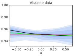
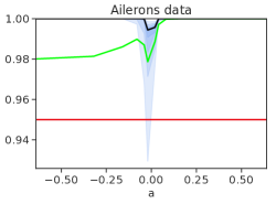
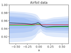
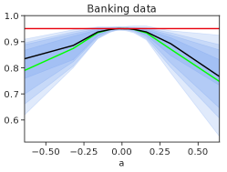
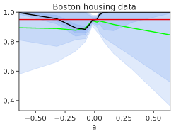
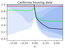
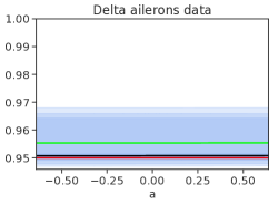
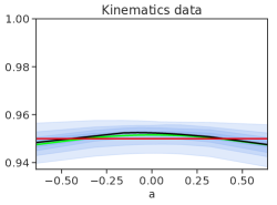
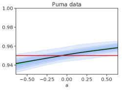
Figure 1: Empirical coverage for the prediction sets generated by the standard conformal methodology across nine regression data sets and 50 random splits of each data set, with an exponential tilting in $X$ space along the first principal component of $X$. The horizontal axis gives the value of the tilting parameter $a$; the vertical the coverage level. A green line marks the average coverage, a black line marks the median coverage, and the horizontal red line marks the nominal coverage $.95$. The blue bands show the coverage at deciles over 50 splits.

Figure 1 presents the results: even when the covariate shifts are small, which corresponds to tilting parameters $a$ with small magnitude, prediction intervals from the standard conformal methodology frequently fail to cover (sometimes grossly) the true response values. While this is but a simple motivation, if we expect some shift in future data—say along the directions of principal variation in $X$, as the data itself is already variable along that axis—it seems that standard validation approaches [44, 20] provide too rosy of a picture of future validity [35], as they enforce exchangeability by randomly splitting data.

2 Robust predictive inference

Of course, standard cross validation and conformalization methodology makes no claims of validity without exchangeability [51, 2, 44], so their potential failure even under simple covariate shifts is not completely surprising. The coverage (4) relies on the exchangeability assumption between the training and test data and can quickly collapse when the test distribution violates that assumption, as Section 1.3 shows. These observations thus call for a notion of confidence more robust to potential future shifts.

Assume as usual that we have a score function $s:\mathcal{X}\times\mathcal{Y}\to\mathbb{R}$, and observe data $\{(X_{i},Y_{i})\}_{i=1}^{n}$ such that $\{S_{i}\}_{i=1}^{n}\coloneqq\{s(X_{i},Y_{i})\}_{i=1}^{n}\stackrel{{\scriptstyle\rm iid}}{{\sim}}P_{0}$, so that $P_{0}$ is the push-forward of $(X,Y)\sim Q_{0}$ under $s(X,Y)$. For a set $\mathcal{P}(P_{0})$ of potential future score distributions on $\mathbb{R}$, our goal is to achieve coverage (1) for all distributions $Q$ on pairs $(X,Y)$ that induce a distribution $P$ on $s(X,Y)$ such that $P\in\mathcal{P}(P_{0})$, that is,

$$Q\in\mathcal{Q}(s,\mathcal{P}(P_{0}))\coloneqq\left\{Q~{}\mbox{s.t.~{}for}~{}(X,Y)\sim Q,\mbox{the score}~{}s(X,Y)\sim P\in\mathcal{P}(P_{0})\right\}.$$

Our focus is exclusively on validating our predictive model, not changing it, so we follow standard practice [51, 2] and use confidence sets $\widehat{C}(x)$ to be of the form $\widehat{C}(x)=\{y\in\mathcal{Y}\mid s(x,y)\leq t\}$ for a threshold $t\in\mathbb{R}$. For such confidence sets, the choice $t\coloneqq\max_{P\in\mathcal{P}(P_{0})}\textup{Quantile}(1-\alpha,P)$ is the smallest $q\in\mathbb{R}$ such that $P(S\leq q)\geq 1-\alpha$ for every distribution $P\in\mathcal{P}(P_{0})$ of the scores. Our general problem to achieve coverage (1) with uncertainty set $\mathcal{Q}(s,\mathcal{P}(P_{0}))$ thus reduces to the optimization problem

$$\mathop{\rm maximize}~{}\textup{Quantile}(1-\alpha;\,P)~{}~{}~{}\mathop{\rm subject\;to}~{}P\in\mathcal{P}(P_{0}).$$ (5)

In the next section, we characterize solutions to this problem, showing in Section 2.2 how to use the characterizations to achieve coverage on future data.

2.1 Characterizing and computing quantiles over $f$-divergence balls

It remains to specify a set of distributions $\mathcal{P}(P_{0})$ that makes problem (5) computationally tractable and statistically meaningful. We thus consider various restrictions on the likelihood ratio $dP/dP_{0}$ for $P\in\mathcal{P}(P_{0})$. Following the distributionally robust optimization literature (DRO) [4, 39, 6, 15, 17, 42], we consider $f$-divergence balls. Given a closed convex function $f:\mathbb{R}\to\mathbb{R}$ satisfying $f(1)=0$ and $f(t)=+\infty$ for $t<0$, the $f$-divergence [12] between probability distributions $P$ and $Q$ on a set $\mathcal{Z}$ is

$$D_{f}\left({P}|\!|{Q}\right)\coloneqq\int_{z\in\mathcal{Z}}f\left(\frac{dP(z)}{dQ(z)}\right)dQ(z).$$

Jensen’s inequality guarantees that $D_{f}\left({P}|\!|{Q}\right)\geq 0$ always, and familiar examples include $f(z)=z\log z$, which induces the KL-divergence, and $f(t)=\frac{1}{2}(t-1)^{2}$, which gives the $\chi^{2}$-divergence. We study problem (5) in the case where $\mathcal{P}(P_{0})$ is an $f$-divergence ball of radius $\rho$ around $P_{0}$:

$$\mathcal{P}_{f,\rho}(P_{0})\coloneqq\left\{P~{}\mbox{s.t.}~{}D_{f}\left({P}|\!|{P_{0}}\right)\leq\rho\right\}.$$ (6)

Unlike most work in the DRO literature, instead of trying to build a model minimizing a DRO-type loss, we assume we already have a model and wish to robustly validate it: to provide predictive confidence sets that are valid and robust to distribution shifts no matter the model’s form. By the data processing inequality, all distributions $Q$ on $(X,Y)$ satisfying $D_{f}({Q}|\!|{Q_{0}})\leq\rho$ induce a distribution $P$ on $s(X,Y)$ satisfying $D_{f}({P}|\!|{P_{0}})\leq\rho$, so solving problem (5) with $\mathcal{P}_{f,\rho}(P_{0})$ provides coverage for all sufficiently small shifts on $(X,Y)\sim Q_{0}$.

We show how to solve problem (5) for fixed $f$ and $\rho$ defining the constraint (6) by characterizing worst-case quantiles, essentially reducing the problem to a one-parameter (Bernoulli) problem. The choice of $f$ and $\rho$ determine plausible amounts of shift—appropriate choices are a longstanding problem [15]—and we defer approaches for selecting them to the sequel. For $\alpha\in(0,1)$ and any distribution $P$ on the real line, we define the $(\alpha,\rho,f)$-worst-case quantile

$$\textup{Quantile}^{\textup{WC}}_{f,\rho}(\alpha;P)\coloneqq\sup_{D_{f}({P_{1}}|\!|{P})\leq\rho}\textup{Quantile}(\alpha;\,P_{1}).$$ (7)

Key to our results both and on valid coverage in Section 2.2 is that this worst-case quantile is a standard quantile of $P$ at a level that depends only on $f,\rho$, and $\alpha$, but not on $P$.

Proposition 1.

Define the function $g_{f,\rho}:[0,1]\to[0,1]$ by

$$g_{f,\rho}(\beta)\coloneqq\inf\left\{z\in[0,1]:\beta f\left(\frac{z}{\beta}\right)+(1-\beta)f\left(\frac{1-z}{1-\beta}\right)\leq\rho\right\}.$$

Then the inverse

$$g_{f,\rho}^{-1}(\tau)=\sup\{\beta\in[0,1]:g_{f,\rho}(\beta)\leq\tau\}$$

guarantees that for all distributions $P$ on $\mathbb{R}$ and $\alpha\in(0,1)$,

$$\textup{Quantile}^{\textup{WC}}_{f,\rho}(\alpha;P)=\textup{Quantile}(g_{f,\rho}^{-1}(\alpha);P).$$

See Appendix A.1 for a proof of the proposition.

Proposition 1 shows that it is easy to compute $g_{f,\rho}$ and $g_{f,\rho}^{-1}$, as they are both solutions to one-dimensional convex optimization problems and therefore admit efficient binary search procedures. In some cases, we have closed forms; for example $f(t)=(t-1)^{2}$ gives $g_{f,\rho}(\beta)=[{\beta-\sqrt{2\rho\beta(1-\beta)}}]_{+}$, while $f(t)=\left|t-1\right|$ yields $g_{f,\rho}(\beta)=(\beta-\rho/2)_{+}$. Another example:

Example 1 (Total variation distances):  The total variation distance $\left\|{P-Q}\right\|_{\rm TV}$ corresponds to the choice $f(t)=|t-1|$ via the identity $2\left\|{P-Q}\right\|_{\rm TV}=D_{f}\left({P}|\!|{Q}\right)$. For this case, we see immediately that $g_{f,\rho}^{-1}(\tau)=\min\{\tau+\frac{\rho}{2},1\}$, and then $g_{f,\rho}(\beta)=\left[{\beta-\rho/2}\right]_{+}$. $\Diamond$ Letting $g=g_{f,\rho}$ for shorthand, we sketch how to compute $g^{-1}$ efficiently in more generality. Computing the inverse $g^{-1}(\tau)$ is equivalent to solving the optimization problem

$$\mathop{\rm maximize}_{0\leq\beta,z\leq 1}~{}\beta~{}~{}~{}\mathop{\rm subject\;to}~{}z\leq\tau,~{}~{}\beta f\left(\frac{z}{\beta}\right)+(1-\beta)f\left(\frac{1-z}{1-\beta}\right)\leq\rho.$$

We seek the largest $\beta\geq\tau$ feasible for this problem (as $\beta=\tau$ is feasible); because $h(\beta,z)=\beta f(z/\beta)+(1-\beta)f((1-z)/(1-\beta))$ is convex and minimized at any $z=\beta$ with $h(z,z)=0$, for $\beta\geq\tau$ it is evident that $\inf_{0\leq z\leq\tau}h(\beta,z)=h(\beta,\tau)$. Thus may equivalently write

$$g^{-1}_{f,\rho}(\tau)=\sup\left\{\beta\in[\tau,1]\mid\beta f\left(\frac{\tau}{\beta}\right)+(1-\beta)f\left(\frac{1-\tau}{1-\beta}\right)\leq\rho\right\},$$

which a binary search over feasible $\beta\in[\tau,1]$ solves to accuracy $\epsilon$ in time $\log\frac{1-\tau}{\epsilon}$.

2.2 Achieving coverage with empirical estimates

With the characterization of $\textup{Quantile}^{\textup{WC}}$, we can define the corresponding prediction set

$$C_{f,\rho}(x;P)\coloneqq\{y\in\mathcal{Y}\mid s(x,y)\leq\textup{Quantile}^{\textup{WC}}_{f,\rho}(1-\alpha;P)\}.$$ (8)

As we observe only a sample $\{S_{i}\}_{i=1}^{n}\stackrel{{\scriptstyle\rm iid}}{{\sim}}P_{0}$, we use the empirical plug-in to develop confidence sets (8) (and therefore in problem (5)), considering $\widehat{C}_{n,f,\rho}(x)\coloneqq C_{f,\rho}(x;\hat{P}_{n})$. By doing this, Proposition 1 allows us to derive guarantees for the prediction set (8) from standard quantile statistics. In particular, the next proposition, whose proof we give in Appendix A.2, lower bounds future coverage conditionally on the validation set $\{(X_{i},Y_{i})\}_{i=1}^{n}$ and relates future test coverage to the amount of shift.

Proposition 2.

Let $S_{n+1}=s(X_{n+1},Y_{n+1})\sim P_{\textup{test}}$ be independent of $\{S_{i}\}_{i=1}^{n}\stackrel{{\scriptstyle\rm iid}}{{\sim}}P_{0}$, and let $\rho^{\star}=D_{f}({P_{\textup{test}}}|\!|{P_{0}})\in\left[{0},{\infty}\right)$. Let $F_{0}$ be the c.d.f. of $P_{0}$. Then the confidence set $\widehat{C}_{n,f,\rho}(x)\coloneqq C_{f,\rho}(x;\hat{P}_{n})$ satisfies

$$\mathbb{P}\left(Y_{n+1}\in\widehat{C}_{n,f,\rho}(X_{n+1})\mid\{(X_{i},Y_{i})\}_{i=1}^{n}\right) \geq g_{f,\rho^{\star}}\left(F_{0}\big{(}\textup{Quantile}^{\textup{WC}}_{f,\rho}(1-\alpha;\hat{P}_{n})\big{)}\right)$$

$$=g_{f,\rho^{\star}}\left(F_{0}\big{(}\textup{Quantile}(g_{f,\rho}^{-1}(1-\alpha);\hat{P}_{n})\big{)}\right).$$

With the two preceding propositions, we turn to the main coverage theorem and a few corollaries, which provide the validity of coverage as long as the true shift between $P_{0}$ and $P_{\textup{test}}$ is no more than our guess. We provide the proof of the theorem in Appendix A.3.

Theorem 1.

Assume that $S_{n+1}=s(X_{n+1},Y_{n+1})\sim P_{\text{test}}$ is independent of $\{S_{i}\}_{i=1}^{n}\stackrel{{\scriptstyle\rm iid}}{{\sim}}P_{0}$, and let $\rho^{\star}=D_{f}({P_{\text{test}}}|\!|{P_{0}})<\infty$. Then

$$\mathbb{P}\left(Y_{n+1}\in\widehat{C}_{n,f,\rho}(X_{n+1})\right)\geq g_{f,\rho^{\star}}\left(\frac{\left\lceil{ng_{f,\rho}^{-1}(1-\alpha)}\right\rceil}{n+1}\right).$$

The theorem as stated is a bit unwieldy, so we develop a few corollaries, whose proofs we provide in Appendix A.4. In each, we assume that the $\rho$ we use to construct the confidence sets (8) satisfies $\rho\geq\rho^{\star}=D_{f}({P_{\text{test}}}|\!|{P_{0}})$, which guarantees validity.

Corollary 2.1.

Let the conditions of Theorem 1 hold, but additionally assume that $\rho^{\star}=D_{f}({P_{\text{test}}}|\!|{P_{0}})\leq\rho$. Then for $c_{\alpha,\rho,f}\coloneqq g_{f,\rho}^{-1}(1-\alpha)g_{f,\rho}^{\prime}(g_{f,\rho}^{-1}(1-\alpha))<\infty$, we have

$$\mathbb{P}\left(Y_{n+1}\in\widehat{C}_{n,f,\rho}(X_{n+1})\right)\geq 1-\alpha-\frac{c_{\alpha,\rho,f}}{n+1}.$$

If instead we replace $\alpha$ in the definition (8) of the confidence set $C_{f,\rho}(x;P)$ with

$$\alpha_{n}\coloneqq 1-g_{f,\rho}\left((1+1/n)g_{f,\rho}^{-1}(1-\alpha)\right)=\alpha-O(1/n),$$

we can construct the corrected empirical confidence set

$$\widehat{C}_{n,f,\rho}^{\textup{corr}}(x)\coloneqq\left\{y\in\mathcal{Y}\mid s(x,y)\leq\textup{Quantile}^{\textup{WC}}_{f,\rho}(1-\alpha_{n};\hat{P}_{n})\right\}.$$

We then have the correct level $\alpha$ coverage:

Corollary 2.2.

Let the conditions of Corollary 2.1 hold. Then

$$\mathbb{P}\left(Y_{n+1}\in\widehat{C}_{n,f,\rho}^{\textup{corr}}(X_{n+1})\right)\geq 1-\alpha.$$

An easier corollary is immediate via Example 1, which shows that when the data distribution changes in variation distance by at most $\rho$, we have (nearly) correct coverage by an identical increase in the choice of quantile level:

Corollary 2.3.

Let $f(t)=|t-1|$. Then

$$\widehat{C}_{n,f,\rho}(x)\coloneqq\left\{y\in\mathcal{Y}\mid s(x,y)\leq\textup{Quantile}\left(1-\alpha+\frac{\rho}{2};\hat{P}_{n}\right)\right\}$$

and if $2\left\|{P_{\text{test}}-P_{0}}\right\|_{\rm TV}\leq\rho$, then

$$\mathbb{P}\left(Y_{n+1}\in\widehat{C}_{n,f,\rho}(X_{n+1})\right)\geq 1-\alpha-\frac{1}{n}.$$

Summarizing, the empirical prediction sets $\widehat{C}_{n,f,\rho}$ and $\widehat{C}^{\textup{corr}}_{n,f,\rho}$ achieve nearly or better than $1-\alpha$ coverage if the $f$-divergence between the new distribution $P_{\text{test}}$ and the current distribution $P_{0}$ remains below $\rho$. When this fails, Theorem 1 shows graceful degradation in coverage as long as the divergence between $P_{\text{test}}$ and the validation population $P_{0}$ is not too large.

2.3 Towards more general uncertainty sets

We now provide an alternative characterization of $\textup{Quantile}^{\textup{WC}}$ that also adapts to other types of uncertainty sets. Our jumping off point is the quantile definition (7): for any continuous distribution $P$, observe that

$$\sup_{D_{f}({P_{1}}|\!|{P})\leq\rho}\textup{Quantile}(1-\alpha;\,P_{1}) =\sup_{D_{f}({P_{1}}|\!|{P})\leq\rho}\inf_{t\in\mathbb{R}}\Bigg{\{}t:P_{1}(s(X,Y)\leq t)\geq 1-\alpha\Bigg{\}}$$

$$\overset{(i)}{=}\sup_{D_{f}({P_{1}}|\!|{P})\leq\rho}\sup_{t\in\mathbb{R}}\Bigg{\{}t:P_{1}(s(X,Y)>t)>\alpha\Bigg{\}}$$

$$=\sup_{t\in\mathbb{R}}\Bigg{\{}t:\sup_{D_{f}({P_{1}}|\!|{P})\leq\rho}\Big{\{}\mathbb{E}_{P_{1}}\big{[}1\!\left\{s(X,Y)>t\right\}\big{]}\Big{\}}>\alpha\Bigg{\}},$$ (9)

where equality $(i)$ follows from the fact that for all $t\in\mathbb{R}$, $t<\textup{Quantile}(1-\alpha,P)$ if and only if $P(S\leq t)<1-\alpha$, i.e. if and only if $P(S>t)>\alpha$.

Efficient computation for Wasserstein balls. This simple duality result (9) gives us an avenue for computing the worst-case quantile w.r.t. different uncertainty sets. For example, if we replace the $f$-divergence ball $D_{f}({P_{1}}|\!|{P})$ appearing in our derivations above with the $p$-Wasserstein distance ball $W_{p}(P_{1},P)$, then we need only replace the above inner maximization problem in (9) with

$$\mathop{\rm maximize}_{W_{p}(P_{1},P)\leq\rho}~{}P_{1}\left[S>t\right],$$ (10)

and we can then still perform the outer maximization via bisection. Problem (10) aims to transport as much mass as possible to $t+\varepsilon$ for some infinitesimal $\varepsilon>0$, and hence is equivalent to the maximization program

$$\mathop{\rm maximize}_{w:\mathbb{R}\to[0,1]}~{}\mathbb{E}_{P}\left[w(S)\right]~{}\mathop{\rm subject\;to}~{}\mathbb{E}_{P}\left[(t-S)_{+}^{p}w(S)\right]\leq\rho^{p}.$$

Letting $t^{\star}\in\mathbb{R}\cup\{-\infty\}$ and $w\in[0,1]$ solve the equation

$$\mathbb{E}_{P}\left[(t-S)_{+}^{p}\left(1\!\left\{S>t^{\star}\right\}+w1\!\left\{S=t^{\star}\right\}\right)\right]=\rho^{p},$$

we see that the solution is $w^{\star}(s)\coloneqq 1\!\left\{s>t^{\star}\right\}$ for $s\neq t^{\star}$ and $w^{\star}(t^{\star})=w$.

3 Procedures for estimating future distribution shift

While the results in the previous section apply for a fixed shift amount $\rho$, a fundamental challenge is—given a validation data set—to determine the amount of shift against which to protect. We suggest a methodology to identify shifts motivated by two (somewhat oppositional) perspectives: first, the variability in predictions in current data is suggestive of the amount of variability we might expect in the future; second, from the perspective of protection against future shifts, that there is no reason future data would not shift as much as we can observe in a given validation set. As a motivating thought experiment, consider the case that the data is a mixture of distinct sub-populations. Should we provide valid coverage for each of these sub-populations, we expect our coverage to remain valid if the future (test) distribution remains any mixture of the same sub-populations. In empirical risk minimization (ERM)-based models, we expect rarer sub-populations to have higher non-conformity scores than average, and building on this intuition, our procedures look for regions in validation data with high non-conformity scores, choosing $\rho$ to give valid coverage in these regions.

We adopt a two-step procedure to describe the set of shifts we consider. Abstractly, let $\mathcal{V}$ be a (potentially infinite) set indexing “directions” of possible shifts, and to each $v\in\mathcal{V}$ associate a collection $\mathcal{R}_{v}$ of subsets of $\mathcal{X}$. (Typically, we either take $\mathcal{V}\subset\mathbb{R}^{d}$ when $\mathcal{X}\subset\mathbb{R}^{d}$, or $\mathcal{V}$ a subset of functions of $\mathcal{X}$, with each $\mathcal{R}_{v}$ then a collection of level sets). For each $R\in\mathcal{R}\coloneqq\bigcup_{v\in\mathcal{V}}\mathcal{R}_{v}\subset\mathcal{P}(\mathcal{X})$, we consider the shifted distribution

$$dQ_{R}(x,y)=\frac{1\!\left\{x\in R\right\}}{Q_{0}(X\in R)}dQ_{0}(x,y)=dQ_{0}(x,y\mid x\in R),$$ (11)

which restricts $X$ to a smaller subset $R$ of the feature space without changing the conditional distribution of $Y\mid X$. The intuition behind the approach is twofold: first, conditionally valid predictors remain valid under covariate shifts of only $X$ (so that we hope to identify failures of validity under such shifts), and second, there may exist privileged directions of shift in the $\mathcal{X}$-space (e.g. time in temporal data or protected attributes in data with sensitive features) for which we wish to provide appropriate $1-\alpha$ coverage.

Example 2 (Slabs and Euclidean balls):  Our prototypical example is slabs (hyperplanes) and Euclidean balls, where we take $\mathcal{V}\subset\mathbb{R}^{d}$, both of which have VC-dimension $O(d)$. In the slab case, for $v\in\mathbb{R}^{d}$ we define the collection of slabs orthogonal to $v$,

$$\mathcal{R}_{v}=\left\{\{x\in\mathbb{R}^{d}\mid a\leq v^{T}x\leq b\}~{}\mbox{s.t.}~{}a<b\right\}.$$

In the Euclidean ball case, we consider $\mathcal{R}_{v}=\{\{x\in\mathbb{R}^{d}\mid\left\|{x-v}\right\|_{2}\leq r\}~{}\mbox{s.t.}~{}r>0\}$, the collection of $\ell_{2}$-balls centered at $v\in\mathcal{V}=\mathbb{R}^{d}$. $\Diamond$

Example 3 (Upper-level functional sets):  A more general example takes $\mathcal{V}$ be a collection of real-valued functions, for instance, a reproducing kernel Hilbert space (RKHS). For each $v\in\mathcal{V}$, $\mathcal{R}_{v}$ is then the collection of upper level-sets

$$\left\{\{x\in\mathcal{X}\mid v(x)\geq a\}~{}\mbox{s.t.}~{}a\in\mathbb{R}\right\}.$$

Were $\mathcal{V}$ all measurable functions, this would guarantee coverage under any covariate shift; practically, $\mathcal{V}$ is a (much) smaller collection. $\Diamond$

Given $\delta\in(0,1)$, we define the worst coverage for a confidence set mapping $C:\mathcal{X}\rightrightarrows\mathcal{Y}$ over $\mathcal{R}$-sets of size $\delta$ by

$$\textup{WC}(C,\mathcal{\mathcal{R}},\delta;\,Q)\coloneqq\inf_{R\in\mathcal{R}}\left\{Q\left(Y\in C(X)\mid X\in R\right)~{}\mbox{s.t.}~{}Q(X\in R)\geq\delta\right\}$$ (12)

Our goal is to find a (tight) confidence set $\widehat{C}$ such that $\textup{WC}(\widehat{C},\mathcal{R},\delta;Q_{0})\geq 1-\alpha$, which, in the setting of Section 2, corresponds to choosing $\rho>0$ such that

$$\textup{WC}(\widehat{C}_{n,f,\rho},\mathcal{R},\delta;\,Q_{0})\geq 1-\alpha.$$

That is, we seek $1-\alpha$ coverage over all large enough subsets of $X$-space.

Barber et al. [2] show that one can theoretically construct such a confidence set when the collection of sets $\mathcal{R}$ is not too large, e.g. if it has finite VC-dimension. Unfortunately, the computation of the worst coverage (12) is usually challenging when the dimension $d$ of the problem grows (as in Example 3), as it typically involves minimizing a non-convex function over a $d$-dimensional domain. This makes the estimation of quantity (12) intractable for large $d$ and hints that requiring such coverage to hold uniformly over all directions $v\in\mathcal{V}$ may be too stringent for practical purposes. However, for a fixed $v\in\mathbb{R}^{d}$, both sets $\mathcal{R}_{v}$ in Example 3 admit $O(d\cdot n)$-time algorithms for computing $\textup{WC}(C,\mathcal{R}_{v},\delta;\widehat{Q}_{n})$ for any empirical distribution $\widehat{Q}_{n}$ with support on $n$ points, which in the slab case is the maximum density segment problem [32]. Thus instead of the full worst coverage (12), we typically resort to a slightly weaker notion of robust coverage, where we require coverage to hold for “most” distributions of the form (11). In the next two sections, we therefore consider two approaches: one that samples directions $v\in\mathcal{V}$, seeking good coverage with high probability, and the other that proposes surrogate convex optimization problems to find the worst direction $v$, which we can show under (strong) distributional assumptions is optimal.

3.1 High-probability coverage over specific classes of shifts

Our first approach is to let $\mathbb{P}_{\mathsf{v}}$ be a distribution on $v\in\mathcal{V}$ that models plausible future shifts. A natural desiderata here is to provide coverage with high probability, that is, conditional on $\widehat{C}$, to guarantee that for a hyperparameter $0<\alpha_{\mathsf{v}}<1$ and for $v\sim\mathbb{P}_{\mathsf{v}}$,

$$\mathbb{P}_{\mathsf{v}}\left[\textup{WC}(\widehat{C},\mathcal{R}_{v},\delta;\,Q_{0})\geq 1-\alpha\right]\geq 1-\alpha_{\mathsf{v}}.$$ (13)

Thus with $\mathbb{P}_{\mathsf{v}}$-probability $1-\alpha_{\mathsf{v}}$ over the direction $v$ of shift, the confidence set $\widehat{C}(X)$ provides $1-\alpha$ coverage over all $R\in\mathcal{R}_{v}$ satisfying $Q_{0}(X\in R)\geq\delta$. The coverage (13) becomes more conservative as $\alpha_{\mathsf{v}}$ decreases to $0$, reducing to condition (12) when $\alpha_{\mathsf{v}}=0$.

Before presenting the procedure, we index the confidence sets by the threshold $q$ for the score function $s$, providing a complementary condition via the robust prediction set (8).

Definition 3.1.

For $q\in\mathbb{R}$, the prediction set at level $q$ is

$$C^{(q)}(x)\coloneqq\{y\in\mathcal{Y}\mid s(x,y)\leq q\}.$$

For a distribution $P$ on $\mathbb{R}$, the value $\rho$ provides sufficient divergence for threshold $q$ if

$$C_{f,\rho}(x;P)\supset C^{(q)}(x)~{}\mbox{for~{}all~{}}x\in\mathcal{X}.$$

By the definition (8) of $C_{f,\rho}$ and Proposition 1, we see that $\rho$ gives sufficient divergence for threshold $q$ if and only if

$$\textup{Quantile}^{\textup{WC}}_{f,\rho}(1-\alpha;P)=\textup{Quantile}(g_{f,\rho}^{-1}(1-\alpha;P))\geq q.$$

To output a confidence set $\widehat{C}$ satisfying the high probability worst-coverage (13), we wish to find $q\in\mathbb{R}$ such that $\mathbb{P}_{\mathsf{v}}[\textup{WC}(C^{(q)},\mathcal{R}_{v},\delta;\,Q_{0})\geq 1-\alpha]\geq 1-\alpha_{\mathsf{v}}$. Notably, any choice of $\rho$ satisfying $\textup{Quantile}^{\textup{WC}}_{f,\rho}(1-\alpha;P_{0})\geq q$ yields a prediction set $C_{f,\rho}(\cdot;P_{0})$ that both provides coverage for covariate shifts $Q_{R}$ of the form (11) across most directions $v\in\mathcal{V}$, in agreement with (13), and enjoys the protection against distribution shift we establish in Section 2 for the given value $\rho$ (including against more than covariate shifts). Algorithm 1 performs this using plug-in empirical estimators for $P_{0}$, $Q_{0}$ and $\mathbb{P}_{\mathsf{v}}$.

Algorithm 1 Worst-subset validation procedure

  Input: sample $\{(X_{i},Y_{i})\}_{i=1}^{n}$ with empirical distribution $\hat{Q}_{n}$; score function $s:\mathcal{X}\times\mathcal{Y}\to\mathbb{R}$ with empirical distribution $\hat{P}_{n}$ on $\{s(X_{i},Y_{i})\}_{i=1}^{n}$; levels $\alpha,\alpha_{\mathsf{v}}\in(0,1)$; divergence function $f:\mathbb{R}_{+}\to\mathbb{R}$; smallest subset size $\delta\in(0,1)$; number of sampled directions $k\geq 1.$

  Do: Sample $\{v_{j}\}_{j=1}^{k}\stackrel{{\scriptstyle\rm iid}}{{\sim}}\mathbb{P}_{\mathsf{v}}$, and let $\hat{\mathbb{P}}_{\mathsf{v},k}$ be their empirical distribution and set

$$\widehat{q}_{\delta}\coloneqq\inf\Bigg{\{}q\in\mathbb{R}:\hat{\mathbb{P}}_{\mathsf{v},k}\Big{(}\textup{WC}(C^{(q)},\mathcal{R}_{v},\delta;\,\widehat{Q}_{n})\geq 1-\alpha\Big{)}\geq 1-\alpha_{\mathsf{v}}\Bigg{\}}.$$ (14)

  Set $\hat{\rho}_{\delta}$ to be any sufficient divergence level for threshold $\widehat{q}_{\delta}$.

  Return: confidence set mapping $\widehat{C}:\mathcal{X}\rightrightarrows\mathcal{Y}$ with $\widehat{C}(x)\coloneqq C^{(\widehat{q}_{\delta})}(x)$ or $\widehat{C}(x)\coloneqq C_{f,\hat{\rho}_{\delta}}(x;\hat{P}_{n})$.

We can show that procedure 1 approaches uniform $1-\alpha$ coverage if the subsets in $\mathcal{R}$ have finite VC-dimension.

Assumption A1 (Score continuity).

The distribution of the scores under $P_{0}$ is continuous.

Theorem 2.

Let $\widehat{C}$ be the prediction set Alg. 1 returns. Assume that $\mathcal{R}=\bigcup_{v\in\mathcal{V}}\mathcal{R}_{v}$ has VC-dimension $\textup{VC}(\mathcal{R})<\infty$. Then there exists a universal constant $c<\infty$ such that the following holds. For all $t>0$, defining

$$\alpha_{t,n}^{\pm}\coloneqq\alpha\pm c\sqrt{\frac{\textup{VC}(\mathcal{R})\log n+t}{\delta n}},\;\textrm{ and }\;\delta_{t,n}^{\pm}=\delta\pm c\sqrt{\frac{\textup{VC}(\mathcal{R})\log n+t}{n}},$$

then with probability at least $1-e^{-t}$ over $\{X_{i},Y_{i}\}_{i=1}^{n}\stackrel{{\scriptstyle\rm iid}}{{\sim}}Q_{0}$ and $\{v_{i}\}_{i=1}^{k}\stackrel{{\scriptstyle\rm iid}}{{\sim}}\mathbb{P}_{\mathsf{v}}$,

$$\mathbb{P}_{\mathsf{v}}\Big{(}\textup{WC}(\widehat{C},\mathcal{R}_{v},\delta_{t,n}^{+};\,Q_{0})\geq 1-\alpha_{t,n}^{+}\Big{)}\geq 1-\alpha_{\mathsf{v}}-c\sqrt{\frac{1+t}{k}}.$$

If additionally Assumption A1 holds, then

$$\mathbb{P}_{\mathsf{v}}\Big{(}\textup{WC}(\widehat{C},\mathcal{R}_{v},\delta_{t,n}^{-};\,Q_{0})\leq 1-\alpha_{t,n}^{-}\Big{)}\geq\alpha_{\mathsf{v}}-\frac{1}{k}-c\sqrt{\frac{1+t}{k}}.$$

See Appendix B for a proof of the theorem.

Theorem 2 shows that Procedure 1 approaches uniform $1-\alpha$ coverage if the subsets in $\mathcal{R}$ have finite VC-dimension. More precisely, the estimate $\hat{\rho}_{\delta}$ almost achieves the randomized worst-case coverage (13): with probability nearly $1-\alpha_{\mathsf{v}}$ over the direction $v\sim\mathbb{P}_{\mathsf{v}}$, $\widehat{C}$ provides coverage at level $1-\alpha-O(1/\sqrt{n})$ for all shifts $Q_{R}$ (as in Eq. (11)) satisfying $R\in\mathcal{R}_{v}$ and $Q_{0}(X\in R)\geq\delta$. The second statement in the theorem is an insurance against drastic overcoverage: while we cannot guarantee that the worst coverage is always no more than $1-\alpha$, we can guarantee that—if the scores are continuous—then the empirical set $\widehat{C}$ has worst coverage no more than $1-\alpha+O(1/\sqrt{n})$ for at least a fraction $\alpha_{\mathsf{v}}$ of directions $v\sim\mathbb{P}_{\mathsf{v}}$. In a sense, this is unimprovable: if the worst coverage $W=\textup{WC}(C,\mathcal{R}_{v},\delta;Q_{0})$ is continuous in $v$, the best we could expect is that $\mathbb{P}_{\mathsf{v}}(W\geq 1-\alpha)=1-\alpha_{\mathsf{v}}$ while $\mathbb{P}_{\mathsf{v}}(W<1-\alpha)=\alpha_{\mathsf{v}}$.

As a last remark, we note that when the scores are distinct, there is a complete equivalence between thresholds $q$ and divergence levels $\rho$ in Algorithm 1; see Appendix B.1 for a proof.

Lemma 3.1.

Assume that the scores $s(X_{i},Y_{i})$ are all distinct. Define $\rho_{f,\alpha}(q;P)\coloneqq\sup\{\rho\geq 0\mid\textup{Quantile}^{\textup{WC}}_{f,\rho}(1-\alpha;P)\leq q\}$ and let $\widehat{\rho}_{\delta}=\rho_{f,\alpha}(\widehat{q}_{\delta},\hat{P}_{n})$. Then $C^{(\widehat{q}_{\delta})}=C_{f,\widehat{\rho}_{\delta}}(\cdot;\hat{P}_{n})$.

3.2 Finding directions of maximal shift

In this section, we revisit worst potential shifts, designing a methodology to estimate the worst direction and protect against it, additionally providing sufficient conditions for consistency. For a confidence set mapping $C:\mathcal{X}\rightrightarrows{Y}$, we define the worst shift direction

$$v_{\star}(C)\coloneqq\mathop{\rm argmin}_{v\in\mathcal{V}}\textup{WC}(C,\mathcal{R}_{v},\delta;\,Q_{0}),$$ (15)

which evidently satisfies

$$\textup{WC}(C,\mathcal{R}_{v_{\star}(C)},\delta;\,Q_{0})=\textup{WC}(C,\mathcal{R},\delta;\,Q_{0})\coloneqq\inf_{v\in\mathcal{V}}\textup{WC}(C,\mathcal{R}_{v},\delta;\,Q_{0}).$$

If we could identify such a worst direction, and it is consistent across thresholds $q$ in our typical definition $C(x)=\{y\in\mathcal{Y}\mid s(x,y)\leq q\}$ (a strong condition), then the procedures in the preceding sections allow us to choose thresholds to guarantee coverage. The intuition here is that there may exist a direction with higher variance in predictions, for example, time in a temporal system. A more explicit example comes from heteroskedastic regression:

Example 4 (Heteroskedastic regression):  Let the data $(X,Y)\in\mathbb{R}^{d}\times\mathbb{R}$ follow the model

$$Y=\mu^{\star}(X)+h(v_{\textup{var}}^{T}X)\varepsilon$$

where $h:\mathbb{R}\to\mathbb{R}_{+}$ is non-decreasing, $\varepsilon\sim\mathsf{N}(0,1)$ independent of $X$, which generalizes the standard regression model to have heteroskedastic noise, with the noise increasing in the direction $v_{\textup{var}}$. Evidently the oracle (smallest length) conditional confidence set for $Y\mid X=x$ is the interval $[\pm z_{1-\alpha/2}\sqrt{h(v_{\textup{var}}^{T}x)}]$ where $z_{1-\alpha}$ is the standard normal quantile. The standard split conformal methodology (Section 1.1) will undercover for those $x$ such that $v_{\textup{var}}^{T}x$ is large: shifts of $X$ in the direction $v_{\star}=v_{\textup{var}}$ may decrease coverage. $\Diamond$

With this example as motivation, we propose identifying challenging directions for dataset shift by separating those datapoints $(X_{i},Y_{i})$ with large nonconformity scores $s(X_{i},Y_{i})$ from those with lower scores. In principle, one can use any M-estimator find such a discriminator, and we suggest a potential approach in Section 3.2.1. To enable our coming analysis, we elaborate slightly and modify notation to reflect that the scoring function $s_{n}$ may change with sample size $n$. We also refine Definition 3.1 of the confidence sets to explicitly depend on both the threshold $q$ and score function $s$.

Definition 3.2.

For $q\in\mathbb{R}$ and a score $s:\mathcal{X}\times\mathcal{Y}\to\mathbb{R}$, the $s$-prediction set at level $q$ is

$$C^{(q,s)}(x)\coloneqq\{y\in\mathcal{Y}\mid s(x,y)\leq q\}.$$ (16)

We assume in this section that $\mathcal{V}\subset L^{2}(Q_{0,X})$ is an RKHS, or a subset thereof, with associated Hilbert norm $\left\|{\cdot}\right\|_{\mathcal{V}}$, and each collection $\mathcal{R}_{v}$ is as in Example 3. The case where $\mathcal{R}$ is the collection of all half-spaces corresponds to $\mathcal{V}=\left\{x\mapsto v^{T}x\mid v\in\mathbb{R}^{d}\right\}$. Additionally, for every $v\in\mathcal{V}$ we let $F_{v}$ be the cumulative distribution function of $v(X)$ when $X\sim Q_{0,X}$ and $F_{v}^{-}(t)\coloneqq\mathbb{P}(v(X)<t)$ its left-continuous version.

Algorithm 2 Worst-direction validation given a score function

  Input: sample $\{(X_{i},Y_{i})\}_{i=1}^{n}$; score function $s_{n}:\mathcal{X}\times\mathcal{Y}\to\mathbb{R}$ independent of the sample; coverage rate $1-\alpha\in(0,1)$; divergence function $f:\mathbb{R}_{+}\to\mathbb{R}$; smallest subset size $\delta\in(0,1)$, worst direction estimation procedure $\mathcal{M}:(\mathbb{R}\times\mathcal{X})^{\star}\to\mathcal{V}$.

  Initialize: Split sample $\{(X_{i},Y_{i})\}_{i=1}^{n}$ into $\{(X_{i},Y_{i})\}_{i=1}^{n_{1}}$, $\{(X_{i},Y_{i})\}_{i=n_{1}+1}^{n_{1}+n_{2}}$ with empirical distributions $\hat{Q}_{n_{1}}$, and $\hat{Q}_{n_{2}}$ (resp. $\hat{P}_{n_{1}}$ and $\hat{P}_{n_{2}}$ for the scores).

  Do: Estimate the worst direction of shift on the first sample distribution $\hat{Q}_{n_{1}}$:

$$\widehat{v}_{n}\coloneqq\mathcal{M}(\{s_{n}(X_{i},Y_{i}),X_{i}\}_{i=1}^{n_{1}}).$$

  Use the second subsample to set the threshold $\widehat{q}_{\delta}$ to

$$\widehat{q}_{\delta}\coloneqq\inf\left\{q\in\mathbb{R}:\textup{WC}(C^{(q,s_{n})},\mathcal{R}_{\hat{v}_{n}},\delta;\,\hat{Q}_{n_{2}})\geq 1-\alpha\right\}.$$ (17)

  Set $\hat{\rho}_{\delta}\coloneqq\rho_{f,\alpha}(\widehat{q}_{\delta};\hat{P}_{n_{2}})=\sup\{\rho\geq 0\mid\textup{Quantile}^{\textup{WC}}_{f,\rho}(1-\alpha;\hat{P}_{n_{2}})\leq q\}$ as in Lemma 3.1.

  Return: the confidence set mapping $\widehat{C}_{n}(x)=C^{(\widehat{q}_{\delta},s_{n})}(x)=C_{f,\hat{\rho}_{\delta}}(x;\hat{P}_{n_{2}})$.

The intuition behind Algorithm 2 is simple: we seek a direction $v$ in which shifts in $X$ make the given nonconformity score $s_{n}$ large, then guarantee coverage for shifts in that direction and, via the distributionally robust confidence set $C_{f,\hat{\rho}}$ the procedure returns, any future distributional shift for which the distribution $P_{\textup{new}}$ of scores $s(X,Y)$ satisfies $D_{f}\left({P_{\textup{new}}}|\!|{P_{0}}\right)\leq\hat{\rho}$. Because we need only solve a single M-estimation problem—rather than sample a large number of directions $v$ as in Alg. 1—the estimation methodology is more computationally efficient.

3.2.1 Population-level consistency of the worst direction

The consistency of Algorithm 2 with the adequate worst-direction estimation procedure $\mathcal{M}$ still requires strong assumptions, somewhat oppositional to the distribution-free coverage we seek (though again we still have the distributionally robust protections). Yet it is still of interest to understand conditions under which Alg. 2 is consistent; as we show here, in examples such as heteroskedastic regression (Ex. 3.2), this holds. We turn to our assumptions.

A challenge is that the worst direction $v_{\star}(C^{(q,s)})$ may vary substantially in $q$. One condition sufficient to ameliorate this reposes on stochastic orders, where for random variables $U$ and $V$ on $\mathbb{R}^{d}$, we say $U$ stochastically dominates in the upper orthant order $V$, written $U\succeq_{\text{uo}}V$, if $\mathbb{P}(U\geq t)\geq\mathbb{P}(V\geq t)$ for all $t\in\mathbb{R}^{d}$ (see [40, Ch. 6], where this is called the usual stochastic order). Letting $\mathcal{L}$ denote the law of a random variable, we write $\mathcal{L}(U)\succeq_{\text{uo}}\mathcal{L}(V)$ if $U\succeq_{\text{uo}}V$.

Assumption A2.

There is a direction $v^{\star}\in\mathcal{V}$ such that $v^{\star}(X)$ has a continuous distribution and, for all $v\in\mathcal{V}$,

$$\left(s(X,Y),F_{v^{\star}}(v^{\star}(X))\right)\succeq_{\text{uo}}\left(s(X,Y),F_{v}^{-}(v(X))\right).$$

The intuition is that covariate shifts in direction $v^{\star}$ not only increase nonconformity, but that $v^{\star}$ is the worst such direction. Assumption A2 focuses on the dependence (copula) between $s(X,Y)$ and $v(X)$, when $v$ ranges over all potential directions of shift in $\mathcal{V}$, and states that $v^{\star}(X)$ and $s(X,Y)$ are more likely to take on larger values together. It only characterizes $v^{\star}$ up to an increasing transformation, which is desirable as any such transformation leaves the collection $\mathcal{R}_{v}$ of upper-level sets invariant.

Under Assumption A2, confidence sets share the same worst shift $v^{\star}$:

Lemma 3.2.

Let Assumption A2 hold. Then $v^{\star}$ is a worst shift (15) for the confidence set (16), i.e. $v^{\star}\in v_{\star}(C^{(q,s)})$ for all $q\in\mathbb{R}$.

We present the (nearly immediate) proof of Lemma 3.2 in Appendix C.1.1. While Assumption A2 is admittedly strong, the next lemma (whose proof we provide in Appendix C.1.2) shows that it holds for linear shifts in the heteroskedastic regression case of Example 3.2.

Lemma 3.3.

Assume the regression model of Example 3.2, $Y=\mu^{\star}(X)+h(X^{T}v_{\textup{var}})\varepsilon$, with noncomformity score

$$s(x,y)=(y-\mu^{\star}(x))^{2}~{}~{}\mbox{or}~{}~{}s(x,y)=|y-\mu^{\star}(x)|,$$

and let $\mathcal{V}=\{x\mapsto v^{T}x\mid v\neq 0\}$ be the set of linear functions. If $v^{T}X$ has a continuous distribution whenever $v\neq 0$, then $v^{\star}=v_{\textup{var}}$ satisfies Assumption A2.

We also suggest potential procedures for identifying the worst direction of shift under limited computational and statistical power. Ideally, a worst shift direction should allow ranking examples by difficulty, with larger values of $v^{\star}(X)$ corresponding to larger values of $s(X,Y)$. The following lemma, whose proof we provide in Appendix C.1.3, formalizes this intuition, stating that the function $v^{\star}$ maximizes the correspondence of the ranks of $n$ samples $(S_{1},\dots,S_{n})$ and $(v^{\star}(X_{1}),\dots,v^{\star}(X_{n}))$. For ease of notation, we denote $S_{i}\coloneqq s(X_{i},Y_{i})$ when appropriate.

Lemma 3.4.

Let Assumption A2 hold. Given three i.i.d. samples $(X_{1},Y_{1})$, $(X_{2},Y_{2})$ and $(X_{3},Y_{3})$, the worst direction $v^{\star}$ satisfies

$$v^{\star}\in\mathop{\rm argmax}_{v\in\mathcal{V}}\left\{\mathbb{P}\left(S_{1}\geq S_{2},v(X_{1})>v(X_{3})\right)\right\}.$$ (18)

While the natural empirical (finite-sample and non-convex) approximation of the problem (18) enjoys $\sqrt{n}$-consistency, and Sherman [41] characterizes its asymptotic distribution, such statistical consistency often comes at the cost of computational tractability, necessitating alternative approaches [11, 16]. Thus, we reframe our problem as a binary classification problem with label $1\!\left\{S_{1}\geq S_{2}\right\}\in\{0,1\}$ and feature vector $X_{1}\in\mathcal{X}$, and consider the following least squares problem:

$$\mathop{\rm minimize}_{\begin{subarray}{c}v\in\mathcal{V}\end{subarray}}\left\{\mathbb{E}\left[\left(v(X_{1})-1\!\left\{S_{1}\geq S_{2}\right\}\right)^{2}\right]\right\}.$$ (19)

The following lemma, whose proof we provide in Appendix C.1.4, shows that the minimization problem (19) amounts to projecting the function

$$\eta_{S}(x)\coloneqq\mathbb{P}(s(x,Y)\geq s(X^{\prime},Y^{\prime})\mid X=x),$$

where $(X,Y)$ and $(X^{\prime},Y^{\prime})$ are independent, onto $\mathcal{V}\subset L^{2}(Q_{0,X})$.

Lemma 3.5.

The minimization problem (19) is equivalent to

$$\mathop{\rm minimize}_{\begin{subarray}{c}v\in\mathcal{V}\end{subarray}}\mathbb{E}\left[\left(v(X)-\eta_{S}(X)\right)^{2}\right].$$

Additionally, if $\eta_{S}(X)$ has a continuous distribution, and if $(X_{1},Y_{1})$, $(X_{2},Y_{2})$ and $(X_{3},Y_{3})$ are i.i.d. and $\mathcal{F}=\{f:\mathcal{X}\to\mathbb{R}\text{ measurable }\}$, then

$$\eta_{S}\in\mathop{\rm argmax}_{f\in\mathcal{F}}\left\{\mathbb{P}\left[S_{1}\geq S_{2},f(X_{1})>f(X_{3})\right]\right\}.$$

The function $\eta_{S}$ quantifies the “hardness” of an instance $x\in\mathcal{X}$ by comparing the score $s(x,Y)$ to an independent sample $S^{\prime}=s(X^{\prime},Y^{\prime})$: if $F_{S}$ is the c.d.f. of $S$, then $\eta_{S}(x)=\mathbb{E}\left[F_{S}(s(X,Y))\mid X=x\right]$. At the same time, it is the nonparametric analogue of the the maximizers in definition (18).

Moving to the finite-sample case, with a sample $\{(X_{i},Y_{i})\}_{i=1}^{n}$, we solve the following convex minimization problem, with a penalty $\lambda_{n}>0$:

$$\hat{v}_{n,\lambda_{n}}\coloneqq\mathop{\rm argmin}_{v\in\mathcal{V}}\left\{\frac{1}{n(n-1)}\sum_{1\leq i\neq j\leq n}\left(v(X_{i})-1\!\left\{S_{i}\geq S_{j}\right\}\right)^{2}+\lambda_{n}\left\|{v}\right\|_{\mathcal{V}}^{2}\right\}.$$ (20)

Under appropriate conditions on the RKHS $\mathcal{V}$, this method is provably consistent, in the sense that $\hat{v}_{n,\lambda_{n}}$ converges towards $\eta_{S}$ as $n\to\infty$. This also entails that, if Assumption A2 holds for a vector space $\mathcal{V}$ sufficiently large, then $v^{\star}$ must be a non-decreasing function of $\eta_{S}$. We summarize these results in the next proposition, which essentially states that we can asymptotically recover the worst direction up to a non-decreasing function, and whose proof we provide in Appendix C.1.5.

Proposition 3.

Assume that $\mathcal{X}$ is a closed measurable space, and that $\mathcal{V}\subset L^{2}(Q_{0,X})$ is a dense, separable RKHS with a bounded measurable kernel. For any sequence $\lambda_{n}\to 0$ such that $n^{1/4}\lambda_{n}\to\infty$, we have

$$\int_{x\in\mathcal{X}}\left(\hat{v}_{n,\lambda_{n}}(x)-\eta_{S}(x)\right)^{2}dQ_{0,X}(x)\mathop{\stackrel{{\scriptstyle a.s.}}{{\rightarrow}}}0.$$

Additionally, let Assumption A2 hold and $\eta_{S}(X)$ have continuous distribution. Then there exists a non-decreasing function $F=F_{v^{\star}}^{-1}\circ F_{\eta_{S}}$ such that $v^{\star}(X)=F(\eta_{S}(X))$ almost surely.

In our subsequent experiments, with a high-dimensional feature space, we use simpler least-squares and SVM estimators of the scores as a fitting procedure for the worst direction of shift, considering linear shifts only. This parametric approach is admittedly more restrictive, and obtaining consistency requires even stronger distributional assumptions, but we can still show that various M-estimators can identify the direction $v^{\star}$ when Assumption A2 holds. We present one such plausible result here, assuming (i) Assumption A2 holds for $\mathcal{V}$ consisting of linear shifts indexed by unit-norm vectors, (ii) that for some $\Sigma\succ 0$, $\Sigma^{-1/2}X$ is rotationally invariant and has finite second moments, and (iii) that $s(X,Y)$ is nonnegative and satisfies $\mathbb{E}\left[s(X,Y)X\right]\neq 0$, and $\mathbb{E}[s(X,Y)^{2}]<\infty$.

Proposition 4.

Let conditions (i)–(iii) above hold. Then $v^{\star}$ is proportional to the least-squares solution

$$v^{\star}\propto\mathop{\rm argmin}_{v\in\mathbb{R}^{d}}\mathbb{E}\left[\left(s(X,Y)-v^{T}X\right)^{2}\right].$$ (21)

See Appendix C.1.6 for a proof.

Example 3.2 with $X\sim\mathsf{N}(0,\Sigma)$ and typical nonconformity scores satisfies the conditions of Proposition 4. While in more general models least squares estimation need not find the worst shift direction, Proposition 4 suggests it may be a reasonable heuristic.

3.2.2 Asymptotic estimation of the worst direction

With the population level recovery guarantees we establish in Propositions 3 and 4, it is now of interest to understand when we may recover the optimal worst direction and corresponding confidence set $C$ using Algorithm 2, which has access only to samples from the population $Q_{0}$. An immediate corollary of Theorem 2 ensures that, under the same conditions, Algorithm 2 returns a confidence set mapping $\widehat{C}_{n}$ that satisfies, conditionally on $s_{n}$ and $\hat{v}_{n}$ and with probability $1-e^{-t}$ over the second half of the validation data,

$$\textup{WC}(\widehat{C}_{n},\mathcal{R}_{\hat{v}},\delta_{t,n_{2}}^{+};\,Q_{0})\geq 1-\alpha_{t,n_{2}}^{+}~{}\text{and}~{}\textup{WC}(\widehat{C}_{n},\mathcal{R}_{\hat{v}},\delta_{t,n_{2}}^{-};\,Q_{0})\leq 1-\alpha_{t,n_{2}}^{-}.$$ (22)

Recalling the definition (12), it remains to understand how close we can expect the uniform quantity $\textup{WC}(\widehat{C}_{n},\mathcal{R},\delta;\,Q_{0})$ to be to $1-\alpha$. By the bounds (22), if the worst coverage is continuous in $v\in\mathcal{V}$ and $s_{n}$ and $\hat{v}_{n}$ are appropriately consistent, we should expect a uniform $1-\alpha$ coverage guarantee in the limit as $n\to\infty$.

To present such a consistency result, we require a few additional assumptions.

Assumption A3 (Consistency of scores and directions).

As $n\to\infty$, we have

$$\left\|{s_{n}-s}\right\|_{L^{2}(Q_{0})}^{2} \coloneqq\int_{\mathcal{X}\times\mathcal{Y}}\left(s_{n}(x,y)-s(x,y)\right)^{2}dQ_{0}(x,y)=o_{P}(1)~{}~{}\text{and}~{}~{}\left\|{\widehat{v}_{n}-v^{*}}\right\|_{L^{2}(Q_{0,X})}=o_{P}(1).$$

Assumption A4 (Continuous distributions).

For $(X,Y)\sim Q_{0}$, the random variables $s(X,Y)$ and $v^{\star}(X)$ have continuous distributions. Additionally, $\hat{v}_{n}(X)$ has a continuous distribution with probability tending to $1$ as $n\to\infty$.

Assumption A5 (Distinct scores).

The scores are asymptotically distinct in probability,

$$Q_{0}^{n}\left[\mbox{there~{}exist}~{}i,j\in[n],i\neq j~{}\mbox{s.t.}~{}s_{n}(X_{i},Y_{i})=s_{n}(X_{j},Y_{j})\right]\stackrel{{\scriptstyle p}}{{\rightarrow}}0.$$

Assumption A5 is a technical assumption that will typically hold whenever Assumption A4 holds, for example, if $s_{n}$ belongs to a parametric family.

Under these assumptions, Theorem 3 proves that we asymptotically provide uniform coverage at level $1-\alpha$ over all shifts $Q_{R}$, $R\in\mathcal{R}$. See Appendix C.2 for a proof.

Theorem 3.

Let Assumptions A2, A3, and A4 hold. Then Algorithm 2 returns a confidence set mapping $\widehat{C}_{n}$ that satisfies

$$\textup{WC}(\widehat{C}_{n},\mathcal{R},\delta;\,Q_{0})=1-\alpha+u_{n}+\varepsilon_{n}$$

where $u_{n}\geq 0$ and $\varepsilon_{n}\stackrel{{\scriptstyle p}}{{\rightarrow}}0$ as $n\to\infty$. If additionally Assumption A5 holds, then $u_{n}\stackrel{{\scriptstyle p}}{{\rightarrow}}0$.

To conclude, we see that the M-estimation-based Procedure 2 to find the worst shift direction can be consistent. Yet even without the (strong) assumptions Theorem 3 requires, we contend the methodology in Algorithm 2 (and Alg. 1) is valuable: it is important to look for variation in coverage within a dataset and to protect against possible future dataset shifts. In particular, Assumption A2 only ensures that the function $\eta_{S}$ is the worst shift independently of the threshold $q\in\mathbb{R}$, i.e that $\textup{WC}(C^{(q,s)},\mathcal{R}_{\eta_{S}},\delta;\,Q_{0})=\textup{WC}(C^{(q,s)},\mathcal{R},\delta;\,Q_{0})$ for all $q\in\mathbb{R}$, but in general, the function $\eta_{S}$ remains a reasonable estimation target in itself: one can view it as the “average” worst direction over a random choice of threshold $S^{\prime}\sim P_{0}$.

4 Coverage sensitivity under covariate shifts

To this point in the paper, the approaches we take for robustness to distribution shifts may often be conservative. Here, we take a complementary and exploratory viewpoint to identify ways in which a predictor may be sensitive. While coverage guarantees of standard predictive inference methods may fail when new data comes from a shifted distribution (recall Section 1.3), protecting against all possible shifts can lead to conservative predictive sets. It is thus of practical interest to identify the particular directions in which a predictive model is indeed distributionally unstable. We therefore propose a measure that evaluates coverage sensitivity under distribution shifts of interest, and we study this measure’s convergence properties by building on a recent line of work distribution shift sensitivity [23, 45, 19].

For a choice of threshold $t\in\mathbb{R}$, we wish to understand the sensitivity of (mis)-coverage of the predictive set $C^{(t)}$ (as in Eq. (16)) under covariate specific distribution shifts. In distinction from Section 2, where we consider general shifts on the score distribution, we now focus on covariate shift. For an index set $I\subset[d]$, this consists of allowing only the distribution of $X_{I}$ to vary while the conditional distribution of $s(X,Y)$ given $X_{I}$ remains invariant. Thus, if we let $P_{0,I}$ be the distribution of $(s(X,Y),X_{I})$ when $(X,Y)\sim Q_{0}$, we consider shifts of measures on $(S,X_{I})$ belonging to

$$\mathcal{P}_{\textup{cov},I}(\rho,P_{0,I})\coloneqq\left\{P=\mathcal{L}(S,X_{I})~{}\mid~{}P(S\in\cdot\mid X_{I})=P_{0,I}(S\in\cdot\mid X_{I})\text{ and }D_{f}\left({P}|\!|{P_{0,I}}\right)\leq\rho\right\}.$$

Assuming (as we will show is possible) that we can accurately evaluate coverage under such shifts, if a given scoring function $s$ is insensitive, then we gain confidence in the performance of $s$, while scoring functions sensitive to such covariate shifts should give us pause.

4.1 Covariate-specific sensitivity analysis

Our goal here is to estimate scoring model’s sensitivity, which we take to be the mis-coverage of the predictive set function $C^{(t)}$ as the distribution of $(S,X_{I})$ varies within $\mathcal{P}_{\textup{cov},I}(\rho,P_{0,I})$. For shift amounts $\rho\geq 0$ and probability distributions (indexed by $I$) $P_{0,I}$ on $\mathbb{R}\times\mathbb{R}^{I}$, we therefore define the covariate specific sensitivity function

$${\operatorname*{SF}}_{\textup{cov},I}^{(t)}(\rho,P_{0,I})\coloneqq\sup_{P}\left\{\mathbb{E}_{P}[1\!\left\{S>t\right\}]\mid P\in\mathcal{P}_{\textup{cov},I}(\rho,P_{0,I})\right\}.$$

Define the conditional miscoverage function on $\mathbb{R}^{I}$ by

$${\operatorname*{M}}_{P_{0,I}}^{(t)}(x)\coloneqq\mathbb{E}_{P_{0,I}}[1\!\left\{S>t\right\}\mid X_{I}=x],$$ (23)

so we can express the sensitivity function as

$${\operatorname*{SF}}_{\textup{cov},I}^{(t)}(\rho,P_{0,I})=\sup\left\{\mathbb{E}_{P}[{\operatorname*{M}}_{P_{0,I}}^{(t)}(X_{I})]\mid P\in\mathcal{P}_{\textup{cov},I}(\rho,P_{0,I})\right\},$$ (24)

as the covariate shift only affects the marginal distribution of $X_{I}\in\mathbb{R}^{I}$ by assumption.

The goal is to leverage equation (24) to build a consistent estimator of the sensitivity function. Given a sample $\{S_{i},X_{I,i}\}_{i=1}^{n}\stackrel{{\scriptstyle\rm iid}}{{\sim}}P_{0,I}$, a natural approach is to follow a two step procedure, by first computing an estimate $\widehat{\operatorname*{M}}_{n_{1}}^{(t)}$ of the miscoverage function using the first $n_{1}$ points, and then approximating the sensitivity function with the remaining $n_{2}=n-n_{1}$ data points, forming the naive estimate

$$\widehat{\operatorname*{SF}}_{\textup{naive},I}(\rho)\coloneqq\sup_{Q}\left\{\mathbb{E}_{X_{I}\sim Q}\big{[}\widehat{\operatorname*{M}}_{n_{1}}^{(t)}(X_{I})\big{]}\text{ s.t. }D_{f}({Q}|\!|{\hat{Q}_{n_{2},I}})\leq\rho\right\},$$

where $\hat{Q}_{n_{2},I}$ is the empirical distribution of $\{X_{I,i}\}_{n_{1}<i\leq n}$.

Unfortunately, if $\widehat{\operatorname*{M}}_{n_{1}}^{(t)}$ converges to $\operatorname*{M}_{P_{0,I}}^{(t)}$ at a slower rate than $\sqrt{n}$, we expect the same behavior from $\widehat{\operatorname*{SF}}_{\textup{naive},I}$, so we take a different tack. In the next section, we show instead how, given an additional (large) sample of unlabeled data $\{X_{i}\}_{i=1}^{N}$, we can achieve a $\sqrt{n}$-consistent asymptotically normal estimate of ${\operatorname*{SF}}_{\textup{cov},I}^{(t)}$ using a debiasing correction [9, 23, 45]. A trade-off is that our debiasing typically leads to a loss of monotonicity of the estimate $\widehat{\operatorname*{SF}}_{\text{cov},I,n}^{(t)}$ in the parameter $\rho\geq 0$. For clarity we focus on a particular limiting divergence, the Rényi $\infty$-divergence

$$D_{\infty}\left({P}|\!|{Q}\right)\coloneqq\lim_{k\to\infty}\frac{1}{k-1}\log\left\{\int\left(\frac{dP(z)}{dQ(z)}\right)^{k}dQ(z)\right\}=\log\operatorname*{ess\,sup}_{Q}\left\{\frac{dP}{dQ}\right\}.$$

A quick calculation shows this corresponds to distribution balls of the form

$$\{P:D_{\infty}\left({P}|\!|{P_{0,I}}\right)\leq\rho\}=\{P\mid\text{ there exists }P_{1,I}\text{ s.t. }P_{0,I}=e^{-\rho}P+(1-e^{-\rho})P_{1,I}\},$$

which offers a simpler dual representation for the sensitivity function (24):

Lemma 4.1 (Example 3, Duchi and Namkoong [15]).

Let $\mathcal{P}_{\textup{cov},I}$ be defined via the Rényi divergence $D_{\infty}$. Then the sensitivity function ${\operatorname*{SF}}_{\textup{cov},I}^{(t)}(\rho,P_{0,I})$ satisfies

$${\operatorname*{SF}}_{\textup{cov},I}^{(t)}(\rho,P_{0,I})=\inf_{\eta\in\mathbb{R}}\bigg{\{}e^{\rho}\mathbb{E}_{P_{0,I}}\left[\left[{{\operatorname*{M}}_{P_{0,I}}^{(t)}(X_{I})-\eta}\right]_{+}\right]+\eta\bigg{\}}.$$

4.2 Cross-fit dual estimation of the sensitivity function

We develop a debiased cross-fit estimator of ${\operatorname*{SF}}_{\textup{cov},I}^{(t)}$ using the representation in Lemma 4.1 and an additional unlabeled sample of covariates $X$, which helps to estimate expectations of the form $\mathbb{E}[\left[{M(X)-\eta}\right]_{+}]$. To build intuition, consider an (abstract) functional of the form in Lemma 4.1, so that for a function $M:\mathcal{X}\to\mathbb{R}$ and $\eta\in\mathbb{R}$ we wish to estimate

$$F_{\rho}(M,\eta)\coloneqq\mathbb{E}\left[e^{\rho}\left[{M(X)-\eta}\right]_{+}\right]+\eta.$$

Consider a first-order expansion of $F_{\rho}$ around $M_{0},\eta_{0}$, where $M_{0}(x)=\mathbb{P}(S>t\mid X=x)$ (recall Eq. (23)) and $\eta_{0}$ minimizes $\mathbb{E}[e^{\rho}\left[{M_{0}(X)-\eta}\right]_{+}]+\eta$ (as in Lemma 4.1) and is thus the $1-e^{-\rho}$ quantile of $M_{0}$. Then using that the subdifferential $\frac{\partial}{\partial t}\left[{t-\eta}\right]_{+}=1\!\left\{t>\eta\right\}$, we heuristically (ignoring interchanges of differentiation and integration) write

$$F_{\rho}(M,\eta) \approx F_{\rho}(M_{0},\eta_{0})+\mathbb{E}\left[e^{\rho}1\!\left\{M_{0}(X)>\eta_{0}\right\}\left(M(X)-M_{0}(X)+\eta_{0}-\eta\right)\right]+\eta-\eta_{0},$$

and rearranging,

$$F_{\rho}(M_{0},\eta_{0}) \approx F_{\rho}(M,\eta)-\mathbb{E}\left[e^{\rho}1\!\left\{M_{0}(X)>\eta_{0}\right\}\left(M(X)-M_{0}(X)\right)\right]$$

$$\qquad-(\eta-\eta_{0})\left(1-e^{\rho}\mathbb{P}(M_{0}(X)>\eta_{0})\right)$$

$$=F_{\rho}(M,\eta)-e^{\rho}\mathbb{E}\left[1\!\left\{M_{0}(X)>\eta_{0}\right\}\left(M(X)-M_{0}(X)\right)\right],$$

where we used that $\mathbb{P}(M_{0}(X)>\eta_{0})=e^{-\rho}$ by construction. For $(M,\eta)$ “near enough” to $M_{0},\eta_{0}$, we have $\mathbb{E}[1\!\left\{M_{0}>\eta_{0}\right\}(M-M_{0})]\approx\mathbb{E}[1\!\left\{M>\eta\right\}(M-M_{0})]\approx\mathbb{E}[1\!\left\{M>\eta\right\}(M-1\!\left\{S>t\right\})]$. In short, we have sketched that

$$F_{\rho}(M_{0},\eta_{0})\approx F_{\rho}(M,\eta)+\mathbb{E}\left[e^{\rho}1\!\left\{M(X)>\eta\right\}\left(1\!\left\{S>t\right\}-M(X)\right)\right],$$ (25)

for $(M,\eta)$ appropriately near to the population quantities $M_{0},\eta_{0}$. Our idea, then, is to use the first-order term in Eq. (25) to correct an empirical calculation of $F_{\rho}(M,\eta)$.

Using the expansion (25) as motivation, for any pair of functions $h:\mathbb{R}^{+}\times\mathbb{R}^{I}\to\mathbb{R}$ and $m:\mathbb{R}^{I}\to\mathbb{R}$, define the augmentation function $\textrm{A}^{(t)}_{h,m}:\mathbb{R}_{+}\times\mathbb{R}\times\mathbb{R}^{I}\to\mathbb{R}$ by

$$\textrm{A}^{(t)}_{h,m}(\rho,s,x)\coloneqq h(\rho,x)\left(1\!\left\{s>t\right\}-m(x)\right).$$

Let $\mathcal{Q}_{0}(m,\rho)\coloneqq\mathop{\rm argmin}_{\eta\in\mathbb{R}}\big{\{}e^{\rho}\mathbb{E}[\left[{m(X_{I})-\eta}\right]_{+}]+\eta\big{\}}$ be the $1-e^{-\rho}$ quantile of $m(X)$ under $P_{0,I}$. For shorthand, omit the subscript on the miscoverage (23) to write ${\operatorname*{M}}^{(t)}\equiv{\operatorname*{M}}_{P_{0,I}}^{(t)}$, define $\mathcal{Q}^{(t)}(\rho)\coloneqq\mathcal{Q}_{0}({\operatorname*{M}}^{(t)},\rho)$, and choose $h^{(t)}(\rho,x)\coloneqq e^{\rho}1\{{\operatorname*{M}}^{(t)}(x)>\mathcal{Q}^{(t)}(\rho)\}$. Then $\mathbb{E}_{P_{0,I}}[\textrm{A}^{(t)}_{h^{(t)},{\operatorname*{M}}^{(t)}}(\rho,S,X_{I})]=0$, so for all $\rho>0$, Lemma 4.1 shows that

$${\operatorname*{SF}}_{\textup{cov},I}^{(t)}(\rho,P_{0,I}) =e^{\rho}\mathbb{E}\left[\left[{{\operatorname*{M}}^{(t)}(X_{I})-\mathcal{Q}^{(t)}(\rho)}\right]_{+}\right]+\mathcal{Q}^{(t)}(\rho)+\mathbb{E}[\textrm{A}^{(t)}_{h^{(t)},{\operatorname*{M}}^{(t)}}(\rho,S,X_{I})].$$ (26)

Algorithm 3 proceeds by first estimating $\operatorname*{M}^{(t)}$, $\mathcal{Q}^{(t)}$ and $h^{(t)}$ successively, before leveraging equation (26) to form a “debiased” cross-fit estimator of ${\operatorname*{SF}}_{\textup{cov},I}^{(t)}(\rho,P_{0,I})$. As mentioned above, it assumes access to a set of unlabeled examples $\{X_{I,j}\}_{1\leq j\leq N}$ where $N\gg n$, which we use to estimate $\mathcal{Q}^{(t)}$ from ${\operatorname*{M}}^{(t)}$. Intuitively, this allows us to accurately estimate properties of $\sigma(X_{I})$-measurable variables, and it is reasonable in semi-supervised regimes where unsupervised examples are cheaper than labeled data.

We first split the data $\{(S_{i},X_{I,i})\}_{i=1}^{n}\stackrel{{\scriptstyle\rm iid}}{{\sim}}P_{0,I}$ into $B\geq 2$ batches $\mathcal{I}_{1},\dots,\mathcal{I}_{B}$ of size $\frac{n}{B}$. For each batch $b\in[B]$, we form an estimate $\widehat{\operatorname*{M}}^{(t)}_{b}$ of ${\operatorname*{M}}^{(t)}$ using all samples from $[n]\setminus\mathcal{I}_{b}$. Using the pool of unlabeled samples, we then compute an estimate $\widehat{\mathcal{Q}}_{b}^{(t)}(\rho)$ of the quantile $\mathcal{Q}_{0}(\widehat{\operatorname*{M}}^{(t)}_{b},\rho)$ (see step (27)), which then gives the $b$th augmented estimator (28). Average over all $B$ batches gives the final estimator $\widehat{\operatorname*{SF}}^{(t)}_{n}(\rho)$. (The augmentation term $\textrm{A}^{(t)}_{\widehat{h}^{(t)}_{b},\widehat{\operatorname*{M}}^{(t)}_{b}}$ makes $\widehat{\operatorname*{SF}}^{(t)}_{n}(\rho)$ potentially non-monotonic in $\rho$.)

Algorithm 3 Covariate sensitivity estimation

  Input: $B$-fold partition $\cup_{b=1}^{B}\mathcal{I}_{b}=[n]$ of $\{(S_{i},X_{I,i})\}_{i=1}^{n}$ s.t. $\left|\mathcal{I}_{b}\right|=\frac{n}{B}$, unlabeled samples $\{X_{I,j}\}_{1\leq j\leq N}$, fitting procedure $\mathcal{A}:\left(\mathbb{R}\times\mathbb{R}^{I}\right)^{\star}\to\{\mathbb{R}^{I}\to\mathbb{R}\}$.

  for $b\in[B]$ do

     Fit an estimator $\widehat{\operatorname*{M}}^{(t)}_{b}\coloneqq\mathcal{A}\left((S_{i},X_{I,i})_{i\in\mathcal{I}_{b}^{c}}\right)$ of the miscoverage function ${\operatorname*{M}}^{(t)}$.

     Compute the $e^{-\rho}$-approximate quantile of $\widehat{\operatorname*{M}}^{(t)}_{b}$ as

$$\widehat{\mathcal{Q}}_{b}^{(t)}(\rho)\coloneqq\mathop{\rm argmin}_{\eta\in\mathbb{R}}\left\{\sum_{j=1}^{N}\frac{e^{\rho}}{N}\left[{\widehat{\operatorname*{M}}^{(t)}_{b}(X_{I,j})-\eta}\right]_{+}+\eta\right\}.$$ (27)

     Set $\widehat{h}^{(t)}_{b}(\rho,x)\coloneqq e^{\rho}1\{\widehat{\operatorname*{M}}^{(t)}_{b}(x)>\widehat{\mathcal{Q}}_{b}^{(t)}(\rho)\}$.

     Compute the $b$-th fold augmented estimator

$$\widehat{\operatorname*{SF}}^{(q)}_{b,n}(\rho)\coloneqq\frac{1}{\left|\mathcal{I}_{b}\right|}\sum_{i\in\mathcal{I}_{b}}\left\{e^{\rho}\left[{\widehat{\operatorname*{M}}^{(t)}_{b}(X_{I,i})-\widehat{\mathcal{Q}}_{b}^{(t)}(\rho)}\right]_{+}+\textrm{A}^{(t)}_{\widehat{h}^{(t)}_{b},\widehat{\operatorname*{M}}^{(t)}_{b}}(\rho,S_{i},X_{I,i})\right\}+\widehat{\mathcal{Q}}_{b}^{(t)}(\rho).$$ (28)

  end for

  return  

$$\widehat{\operatorname*{SF}}^{(t)}_{n}(\rho)\coloneqq\frac{1}{B}\sum_{b=1}^{B}\widehat{\operatorname*{SF}}^{(t)}_{b,n}(\rho)$$ (29)

4.2.1 Consistency and convergence rate of the augmented estimator $\widehat{\operatorname*{SF}}^{(q)}_{n}$

We study the consistency and rate of covergence of the sensitivity estimator (29) as a path function of $\rho\in\mathbb{R}_{+}$, for which we require a few assumptions below. Assumption A6 states that the fitted estimator $\widehat{\operatorname*{M}}_{b}$ needs to be appropriately consistent for ${\operatorname*{M}}_{P_{0,I}}^{(t)}$, while Assumption A7 basically ensures the pool of unlabeled samples is large enough to provide a good estimate of the quantiles of $\widehat{\operatorname*{M}}_{b}$. Assumption A8 is technical and prevents the random variable ${\operatorname*{M}}_{P_{0,I}}^{(t)}(X_{I})$ from being too concentrated, thus allowing quantile estimation.

Assumption A6 (Miscoverage estimation).

For each batch $b\in[B]$, we have

$$\left\|{\widehat{\operatorname*{M}}^{(t)}_{b}-{\operatorname*{M}}^{(t)}}\right\|_{L^{\infty}(P_{0,I})}=o_{p}(n^{-1/4}).$$

Assumption A7 (Quantile estimation).

For each $b\in[B]$ and every compact $K\subset\mathbb{R}_{+}$, the quantile estimator $\widehat{\mathcal{Q}}_{b}$ satisfies

$$\sup_{\rho\in K}\left|\widehat{\mathcal{Q}}_{b}(\rho)-\mathcal{Q}_{0}(\widehat{\operatorname*{M}}_{b},\rho)\right|=o_{p}(n^{-1/4}).$$

Assumption A8.

The random variable ${\operatorname*{M}}_{P_{0,I}}^{(t)}(X_{I})$ has a bounded density $f_{\operatorname*{M}}$ on $[0,1]$.

Under these assumptions, we have the following theorem, which shows that for every compact set $K\subset\mathbb{R}$, the sequence of processes $\{\sqrt{n}(\widehat{\operatorname*{SF}}^{(t)}_{n}(\rho)-{\operatorname*{SF}}_{\textup{cov},I}^{(t)}(\rho))\}_{\rho\in K}$ converges in distribution in $L^{\infty}(K)$ to a tight Gaussian process, whose covariance is tedious to specify though we characterize it in the proof of the theorem in Appendix D.

Theorem 4.

Let Assumptions A6–A8 hold. Then there exists a tight Gaussian process $\mathbb{G}$ such that, for every compact set $K\subset\mathbb{R}^{+}$, we have

$$\{\sqrt{n}(\widehat{\operatorname*{SF}}^{(t)}_{n}(\rho)-{\operatorname*{SF}}_{\textup{cov},I}^{(t)}(\rho))\}_{\rho\in K}\mathop{\stackrel{{\scriptstyle d}}{{\rightarrow}}}\{\mathbb{G}(\rho)\}_{\rho\in K}~{}~{}~{}\mbox{as~{}elements~{}of~{}~{}}L^{\infty}(K).$$

A few consequences of Theorem 4 are immediate. First, we have $\sqrt{n}$-consistency:

$$\sqrt{n}\cdot\sup_{\rho\in K}|\widehat{\operatorname*{SF}}^{(t)}_{n}(\rho)-{\operatorname*{SF}}_{\textup{cov},I}^{(t)}(\rho))|\mathop{\stackrel{{\scriptstyle d}}{{\rightarrow}}}\sup_{\rho\in K}\mathbb{G}(\rho)$$

as the supremum mapping is continuous in $L^{\infty}$, and so $\|{\widehat{\operatorname*{SF}}^{(t)}_{n}-{\operatorname*{SF}}_{\textup{cov},I}^{(t)}}\|_{\infty}=O_{P}(1/\sqrt{n})$. As another immediate consequence, we see that under the assumptions of Theorem 4, for every $\rho>0$, there exists $\sigma^{2}(\rho)<\infty$ such that

$$\sqrt{n}(\widehat{\operatorname*{SF}}^{(t)}_{n}(\rho)-{\operatorname*{SF}}_{\textup{cov},I}^{(t)}(\rho))\mathop{\stackrel{{\scriptstyle d}}{{\rightarrow}}}\mathsf{N}(0,\sigma^{2}(\rho)).$$

(This is similar to the result [45, Thm. 1], but as we note in footnote 3, the papers [45, 23] may have technical mistakes.)

5 Empirical analysis

Given the challenges arising in the practice of machine learning and statistics, this paper argues that methodology equipping models with a notion of validity in their predictions—e.g., conformalization procedures as in this paper—is essential to any modern prediction pipeline. Section 1.3 illustrates the need for these sorts of procedures, showing that the standard conformal methodology is sensitive to even small shifts in the data, through (semi-synthetic) experiments on data from the UCI repository. In Section 2, we propose methods for robust predictive inference, giving methodology that estimates the amount of shift to which we should be robust. Fuller justification requires a more careful empirical study that highlights both the failures of non-robust prediction sets on real data as well as the potential to handle such shifts using the methodology here. To that end, we turn to experimental work:

• In Section 5.1, we resume the evaluation of our own methodology on the semi-synthetic data from Section 1.3.

• Section 5.2 shows evaluation centered around the new MNIST, CIFAR-10, and ImageNet test sets. These datasets exhibit real-world distributional shifts, and we test whether our methodology of estimating plausible shifts is sufficient to provide coverage in these real-world shifts.

• In Section 5.3, we consider a time series where the goal is to predict the fraction of people testing positive for COVID-19 throughout the United States.

• In Section 5.4, we apply Algorithm 3 to evaluate the sensitivity of predictive methods to individual covariate shifts.

5.1 UCI datasets

We revisit the experiments in Section 1.3, focusing on evaluating our methodology for robust predictive inference. Our goal here is to show that when our estimate of the amount of shift is comparable to the actual amount of shift, our methodology delivers coverage without inflating prediction sets too much. Accordingly, throughout these experiments, we fix the desired robustness level $\rho=.01$, corresponding (approximately) to the median chi-squared divergence between the natural and tilted empirical distributions across the nine data sets and values of the tilting parameter $a$. We therefore expect Algorithm 1, which emphasizes robustness to worst-case shifts, to restore the coverage level for the tiltings from Section 1.3 that possess (roughly) this level of shift.

Figure 2 presents the results for the chi-squared divergence (the results for the Kullback-Leibler divergence are similar). Although not perfect, we see that the methodology often restores validity for the shifts from Section 1.3. We see clearly improved performance over the standard conformal methodology on the abalone, delta ailerons, kinematics, puma, and airfoil datasets (compare to Figure 1). On all of these datasets, the robust methodology consistently yields average coverage above the nominal level, while standard conformal fails to cover on each of the datasets. Treating the test sample as truth, we evaluate the median chi-squared divergence between these natural and shifted distributions across values of the tilting parameter $a$; the divergence values are .03, .02, .04, .05, and 3.65, respectively, while the level of divergence for the remaining datasets (ailerons—which still covers—banking, and Boston and California housing) is roughly twice as large, which explains the loss in coverage. We note in passing that in other experiments we omit for brevity, the trends above hold for other types of shifts.

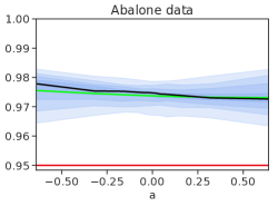
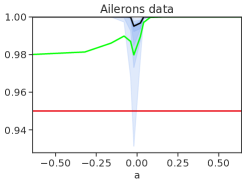
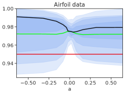
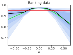
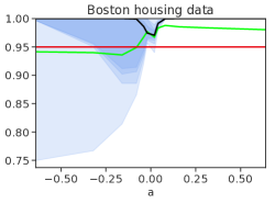
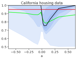
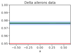
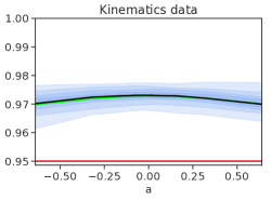
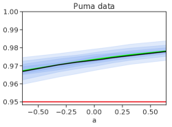
Figure 2: Empirical coverage for the prediction sets generated by the chi-squared divergence, following the same experimental setup from Section 1.3. The horizontal axis gives the value of the tilting parameter $a$; the vertical the coverage level. A green line marks the average coverage, a black line marks the median coverage, and the horizontal red line marks the nominal coverage $.95$. The blue bands show the coverage at various deciles.

5.2 CIFAR-10, MNIST, and ImageNet datasets

We evaluate our procedures on the CIFAR-10, ImageNet, and MNIST datasets [25, 37, 26], which continue to play a central role in the evaluation of machine learning methodology. Concerns about overfitting to these benchmarks motivate Recht, Roelofs, Schmidt, and Shankar [35] to create new test sets for both CIFAR-10 and ImageNet by carefully following the original dataset creation protocol. Though these new test sets strongly resemble the original datasets, as Recht et al. observe, the natural variation arising in the creation of the new test sets yield evidently significant differences, giving organic dataset shifts on which to evaluate our procedures. Our goal here is to show that even when we do not know the actual amount of shift, our methodology from Section 3.1 can still give reasonable estimates of it that translate into marginal coverage on these datasets.

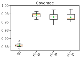
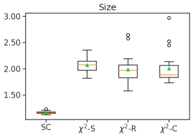
Figure 3: Empirical coverage and average size for the prediction sets generated by the standard conformal methodology (“SC”) and the chi-squared divergence, across 20 random splits of the CIFAR-10 data. We set $\rho$ according to the sampling (“$\chi^{2}$-S”), regression (“$\chi^{2}$-R”), and classification-based (“$\chi^{2}$-C”) strategies for estimating the amount of shift that we describe in Section in 3. The horizontal red line marks the marginal coverage $.95$.

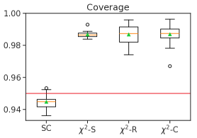
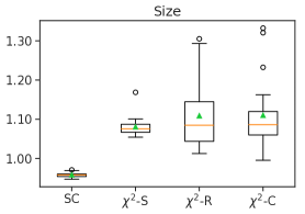
Figure 4: Empirical coverage and average size for the prediction sets generated by the standard conformal methodology (“SC”) and the chi-squared divergence, across 20 random splits of the MNIST data. We set $\rho$ according to the sampling (“$\chi^{2}$-S”), regression (“$\chi^{2}$-R”), and classification-based (“$\chi^{2}$-C”) strategies for estimating the amount of shift that we describe in Section in 3. The horizontal red line marks the marginal coverage $.95$.

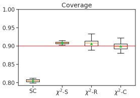
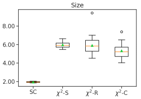
Figure 5: Empirical coverage and average size for the prediction sets generated by the standard conformal methodology (“SC”) and the chi-squared divergence, across 20 random splits of the ImageNet data. We set $\rho$ according to the sampling (“$\chi^{2}$-S”), regression (“$\chi^{2}$-R”), and classification-based (“$\chi^{2}$-C”) strategies for estimating the amount of shift that we describe in Section in 3. The horizontal red line marks the marginal coverage $.9$.

We evaluate on the three datasets as follows. We use 70% of the original CIFAR-10, MNIST, and ImageNet datasets for training, and treat the remaining 30% as a validation set. We fit a standard ResNet-50 [21] to the training data, and use the negative log-likelihood $s(x,y)=-\log p_{\theta}(y\mid x)$, where $p_{\theta}(y\mid x)$ is the output of the (top) sigmoid layer of the network, as the scoring function on the validation data for our conformalization procedures. We compare our procedures to the split conformal methodology on three new datasets nominally generated identically to the initial datasets: the CIFAR-10.1 v4 dataset [35], which consists of 2,000 32$\times$32 images from 10 different classes; the QMNIST50K data, which extends MNIST to consist of 50,000 28$\times$28 images from 10 classes [54]; and the ImageNetV2 Threshold0.7 data [35], consisting of 10,000 images from 200 classes. In each test of robust predictive inference, we set the level of robustness to achieve the nominal coverage $\alpha=.05$ for the CIFAR-10 and MNIST datasets and $\alpha=.1$ for the ImageNet dataset, by using the data-driven strategies that we detail in Section 3: sampling directions of shift from the uniform distribution on the unit sphere (Alg. 1), estimating the shift direction via regression (Alg. 2) or via classification, which replaces the regression step in Alg. 2 with a support vector machine (SVM) to separate the largest 50% of scores $s(X_{i},Y_{i})$ from the smallest. In contrast to our experiments from Section 5.1 with semi-synthetic data, we cannot compute the exact level of shift here; the question is whether the provided methodology provides marginal coverage.

Figures 3, 4, and 5 present the results for each setup over 20 random splits of the data. As is apparent from the figures, we see that the standard conformal methodology fails to correctly cover. As both the new CIFAR-10 and ImageNet test sets exhibit larger degradations in classifier performance (increased error) than does the MNIST test set [35], we expect the failure of standard conformal to be pronounced on these two datasets. Indeed, the split conformal method (Sec. 1.1) provides especially poor coverage on these datasets, where it yields average coverage .88 (instead of the nominal .95) and .8 (instead of the nominal .9) on the new CIFAR-10 and ImageNet test sets, respectively. On the other hand, our inferential methodology consistently gives more coverage regardless of the strategy used to estimate the amount of divergence $\rho$, with the sampling strategy notably consistently delivering marginal coverage without over-covering. The uniformity in coverage across the three strategies is notable, as our procedures for estimating the amount of shift assume some structure for the underlying shift, which is unlikely to be consistent with the provenance of the new test sets.

In our experiments, estimating the direction of shift using either regression or classification (Alg. 2) is faster than sampling directions (Alg. 1); the former takes time $O(nd\min\{n,d\})$ and the latter $O(knd)$, where $k$ is the number of sampled directions $v$, using a linear-time implementation for computing the worst coverage (maximum density segment) along a direction $v$ [32]. The difference of course depends on the desired sampling frequency $k$.

Finally, the aforementioned validity does not (apparently) come with a significant loss in statistical efficiency: Figures 3, 4, and 5 show that our confidence sets are not substantially larger than those coming from standard conformal inference—which may be somewhat surprising, given the relatively large number of classes present in the ImageNet dataset.

5.3 COVID-19 forecasting

Our final evaluation of prediction accuracy under shifts is to predict test positivity rates for COVID-19, in each of $L=3{,}140$ United States counties in a time series over $T=34$ weeks from January through the beginning of August 2021, using demographic features. As a non-stationary time series, robustness is essential here as a fixed model of course cannot adapt to the underlying distributional changes.

Our prediction task is as follows. For each of $t=1,\ldots,T$ weeks, and at each of $\ell=1,\ldots,L$ locations (counties), we observe a real-valued response $Y_{\ell,t}\in[0,1]$, $\ell=1,\ldots,L$, $t=1,\ldots,T$, measuring the fraction of people with COVID-19. We use data from the DELPHI group at Carnegie Mellon University [1, 48] and consider a similar featurization, using the following trailing average features within each county: (1) the number of COVID-19 cases per 100,000 people; (2) the number of doctor visits for COVID-like symptoms; and (3) the number of responses to a Facebook survey indicating respondents have COVID-like symptoms. We standardize both the features and responses so that they lie in $[0,1$], and collect the features into vectors $X_{\ell,t}\in\mathbb{R}^{3}$, $\ell=1,\ldots,L$, $t=1,\ldots,T$.

At each week $t=1,4,7,\ldots$, we fit a simple logistic model where for a fixed $t$, we compute

$$(\hat{\alpha}^{(t)},\hat{\beta}^{(t)})\in\mathop{\rm argmin}_{\alpha\in\mathbb{R},\beta\in\mathbb{R}^{d}}~{}\sum_{\ell=1}^{L}\left[\log(1+e^{\alpha+X_{\ell,t}^{T}\beta})-Y_{\ell,t+1}(\alpha+X_{\ell,t}^{T}\beta)\right]$$ (30)

We treat the data at the weeks $t=2,5,8,\ldots$ as the validation set, the data at the remaining weeks $t=3,6,9,\ldots$ as the test set, so that at each time $t$ we fit the single most recent time period’s data. We make predictions on a new example $x$ at time $t$ via the logistic link

$$\widehat{y}=\frac{e^{\hat{\alpha}^{(t)}+x^{T}\hat{\beta}^{(t)}}}{1+e^{\hat{\alpha}^{(t)}+x^{T}\hat{\beta}^{(t)}}}.$$

For our robust conformalization procedures, we consider the Kullback-Leibler divergence and estimate the divergence $\rho$ between weeks $1,4,7,\ldots$ and $2,5,8,\ldots$ via regression (Alg. 2), as well as with a nonparametric divergence estimator [33]; given this $\rho$ we then make robust predictions at the test times $t=3,6,\ldots$. We compare to the standard split conformal methodology—which is of course not robust to departures from the validation distribution—but also consider the standard conformal methodology with the more conservative miscoverage level $\alpha/2$ to attain robustness to a variation distance shift of $\alpha/2$ (recall Corollary 2.3). We set $\alpha=.1$ throughout these experiments.

Figures 6–9 present the results. From Figure 6, we can see that the standard conformal methodology (once again) fails to cover, whereas our (two) robust conformalization procedures retain validity. These results are in line with our expectations: we expect the standard methodology to undercover as it is not robust to distributional changes, and we expect both Alg. 2 as well as the nonparametric divergence estimator of Nguyen et al. [33] to deliver reasonably accurate estimates of the divergence level $\rho$ given the low ambient dimension of the feature space (recall that $d=3$), translating into generally good coverage here. We can also see that the standard conformal methodology with the conservative miscoverage level $\alpha/2$ gives coverage at roughly the right level, though it is does not adapt the miscoverage level to the problem at hand (as estimating an appropriate level of divergence is an important component). Along these lines, Figure 7 reveals a more complete picture: the heuristic also gives rise to (slightly) longer confidence intervals than most of the other methods—which is intuitive as again we have no guarantee that $\alpha/2$ corresponds to the true amount of divergence between the validation and test distributions. Overall, our robust conformalization procedure combined with Nguyen et al.’s nonparametric divergence estimator [33] appears to strike the best balance between coverage and confidence interval length in this instance.

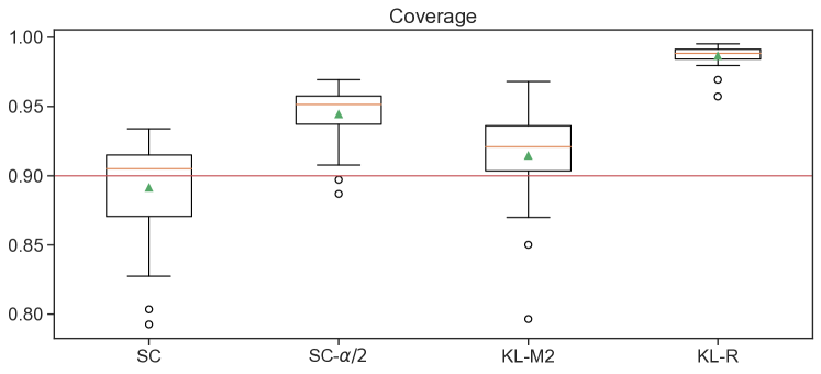
Figure 6: Empirical coverage for the prediction sets generated by the standard conformal methodology (“SC”), the standard conformal methodology where we simply set $\alpha/2$ (“SC-$\alpha/2$”), and the Kullback-Leibler divergence on the COVID-19 time series. We set $\rho$ according to the regression-based strategy (“KL-R”) for estimating the amount of shift that we describe in Section 3.1, as well as via the nonparametric divergence estimator due to Nguyen et al. [33] (“KL-M2”). The horizontal red line marks the marginal coverage $.9$.

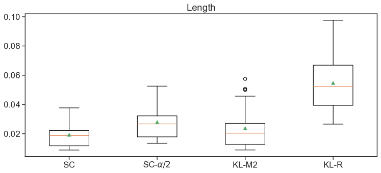
Figure 7: Average length for the prediction intervals generated by the standard conformal methodology (“SC”), the standard conformal methodology where we simply set $\alpha/2$ (“SC-$\alpha/2$”), and the Kullback-Leibler divergence on the COVID-19 time series. We set $\rho$ according to the regression-based strategy (“KL-R”) for estimating the amount of shift, as well as via the nonparametric divergence estimator due to Nguyen et al. [33] (“KL-M2”).

We view these results from a more qualitative perspective in Figures 8 and 9. In Figure 8, we show the actual number of COVID-19 cases on April 16, 2021, when the state of Michigan saw a sudden spike in the incidence of COVID-19 after several weeks of implementing precautionary measures. As an especially pronounced example of distributional shift, it is natural to ask whether our procedures might offer any kind of protection in this instance. Figure 9 shows the upper and lower endpoints of the confidence intervals that our robust conformalization procedure generates at this point in time. By comparing the colors in the figures, we can see that our robust prediction intervals generally contain the true response value both across the United States as well as in Michigan, in particular—despite the presence of such a severe distributional shift.

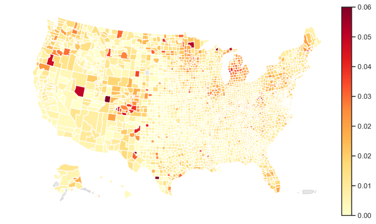
Figure 8: The true (normalized) number of COVID-19 cases per 100,000 people, smoothed over the previous week, across the United States on April 16, 2021.

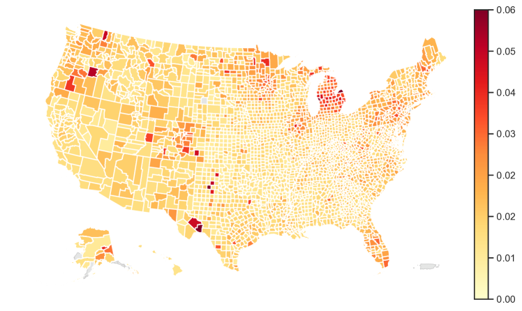
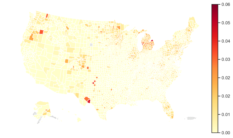
Figure 9: The upper (top panel) and lower (bottom panel) endpoints of the confidence intervals that our robust conformal methodology generates across the United States on April 16, 2021.

5.4 Experiments on covariate sensitivity

Our final experiment is to evaluate our sensitivity predictions for covariate shift, as in Sec. 4. The point is twofold: we (i) identify covariates for which covarage may be sensitive, then (ii) test whether these putative sensitivities are indeed present in data. To do so, we consider three datasets from the UCI repository [13]: real-estate data, weather history data, and wine quality data.

We repeat the following experiment 25 times: we randomly partition each dataset into disjoint sets $D_{\textrm{train}},D_{\textrm{val}},D_{\text{sens}},D_{\textrm{test}}$ each containing respectively $40\%,10\%,30\%,10\%$ of the data, then fit a linear regression model $\mu$ using $D_{\textrm{train}}$ and construct conformal intervals of the form (3) with $s(x,y)=|\mu(x)-y|$, so that $\widehat{C}_{n}(x)=\{y\in\mathbb{R}\mid|\mu(x)-y|\leq\hat{t}\}$, setting the threshold $\hat{t}$ so that we achieve coverage at nominal level $\alpha=.1$ on $D_{\textrm{val}}$. We estimate the sensitivity function using $D_{\text{sens}}$ as in Algorithm 3 for each singleton covariate (i.e. the covariate set $I=\{i\}$ for each of $i=1,2,\ldots$), where we estimate the conditional probabilities of miscoverage using default tuning parameeters in R’s version of random forests.

Figure 10 shows the results. The plot is somewhat complex: for each of the three datasets, we estimate sensitivity (as a function of shift $\rho$) for each covariate in the dataset (e.g. House age in the real estate data). Then for an individual covariate, we plot (estimated) maximum miscoverage as a function of the radius $\rho$ of potential shift in that covariate (the estimated sensitivity function (24), where $I=\{i\}$ is the covariate of interest); this is the red solid line in each plot. As we are curious about coverage losses under covariate shifts, we plot miscoverage (dashed lines) on the subset of the test data $D_{\textrm{test}}$ containing examples either from the upper or lower $e^{-\rho}$ quantiles of each covariate, which corresponds to Rényi $\infty$-divergence $\rho$, as in Lemma 4.1. We expect that these miscoverages to fall below the maximum miscoverage line, which we observe across all three datasets. Specifically, we see that for real estate data, coverage of the corresponding confidence sets drops most when the marginal distribution of the covariate “House age” shifts while that for weather history data, the coverage drops most for shifts in the “Pressure” covariate. For the wine quality dataset, coverage seems almost equally sensitive to all covariates. An interesting question for future work is to identify those directions which are sensitive—as opposed to the approach here, which identifies potentially sensitive covariates.

\begin{overpic}[scale={0.28}]{sensitivity/real-estate.pdf} \put(40.0,-1.0){ \small Real estate data} \put(-1.0,10.0){ \leavevmode\hbox to8.94pt{\vbox to171.12pt{\text{[drawing]}}} } \put(-1.0,25.0){\rotatebox{90.0}{ $\rho$} } \end{overpic}

\begin{overpic}[scale={0.28}]{sensitivity/weather-history.pdf} \put(40.0,-1.0){ \small Weather history data } \put(-1.0,10.0){ \leavevmode\hbox to8.94pt{\vbox to171.12pt{\text{[drawing]}}} } \put(-1.0,20.0){\rotatebox{90.0}{ $\rho$} } \end{overpic}

\begin{overpic}[scale={0.28}]{sensitivity/wine-quality.pdf} \put(40.0,-1.0){ \small Wine quality data } \put(-1.0,10.0){ \leavevmode\hbox to8.94pt{\vbox to171.12pt{\text{[drawing]}}} } \put(-1.0,20.0){\rotatebox{90.0}{ $\rho$} } \end{overpic}

Figure 10: Sensitivity of (mis)-coverage for three datasets. Red line shows maximum miscoverage possible within a given shift in marginal distribution of a covariate with respect to limiting $f$-divergences. Dashed lines show miscoverage on a subset of test data that contains samples for which the corresponding covariate takes values in the upper or lower $e^{-\rho}$ quantiles of that covariate.

6 Discussion and conclusions

We have presented methods and motivation for robust predicitve inference, seeking protection against distribution shift. Our arguments and perspective are somewhat different from the typical approach in distributional robustness [5, 17, 15, 7, 38], as we wish to maintain validity in prediction. A number of future directions and questions remain unanswered. Perhaps the most glaring is to fully understand the “right” level of robustness. While this is a longstanding problem [15], we present approaches to leverage the available validation data. Alternatives might be compare new covariates and test data $X$ to the available validation data. Tibshirani et al. [49] suggest an importance-sampling approach for this, reweighting data based on likelihood ratios, which may sometimes be feasible but is likely impossible in high-dimensional scenarios. It would be interesting, for example, to use projections of the data to match $X$-statistics on new test data, using this to generate appropriate distributional robustness sets. We hope that the perspective here inspires renewed consideration of predictive validity.

Appendix A Proofs of results on robust inference

A.1 Proof of Proposition 1

We provide several properties of $g_{f,\rho}(\beta)=\inf\{z\in[0,1]:\beta f(\frac{z}{\beta})+(1-\beta)f(\frac{1-z}{1-\beta})\leq\rho\}$, deferring their proof to Sec. A.1.1.

Lemma A.1 (Properties of $g_{f,\rho}$).

Let $f$ be a closed convex function such that $f(1)=0$ and $f(t)<\infty$ for all $t>0$. Then the function $g_{f,\rho}$ satisfies the following.

1. $(\beta,\rho)\mapsto g_{f,\rho}(\beta)$ is a convex function.

2. $g_{f,\rho}$ is non-increasing in $\rho$ and non-decreasing in $\beta$. Moreover, for all $\rho>0$, there exists $\beta_{0}(\rho)\coloneqq\sup\{\beta\in(0,1)\mid g_{f,\rho}(\beta)=0\}$, and $g_{f,\rho}$ is strictly increasing for $\beta>\beta_{0}(\rho)$.

3. $(\beta,\rho)\mapsto g_{f,\rho}(\beta)$ is continuous for $\beta\in[0,1]$ and $\rho\in(0,\infty)$.

4. For $\beta\in[0,1]$ and $\rho>0$, $g_{f,\rho}(\beta)\leq\beta$. For $\rho>0$, equality holds for $\beta=0$, strict inequality holds for $\beta\in(0,1)$ and $\rho>0$, and $g_{f,\rho}(1)=1$ if and only if $f^{\prime}(\infty)=\infty$.

5. Let $g_{f,\rho}^{-1}(t)=\sup\{\beta:g_{f,\rho}(\beta)\leq t\}$ as in the statement of Proposition 1. Then for $\beta\in(0,1)$, $g_{f,\rho}(\tau)\geq\beta$ if and only if $g_{f,\rho}^{-1}(\beta)\leq\tau$.

We now define the worst-case cumulative distribution function, which generalizes the c.d.f. of a distribution in the same way the worst-case quantile generalizes standard quantiles.

Definition A.1 ($f$-worst-case c.d.f.).

Let $\rho>0$ and consider any distribution $P$ on the real line. The $(f,\rho)$-worst-case cumulative distribution function is

$$F^{\textup{WC}}_{f,\rho}(t;\,P)\coloneqq\inf\big{\{}P_{1}(S\leq t)\mid S\sim P_{1},\;D_{f}({P_{1}}|\!|{P})\leq\rho\big{\}}.$$ (31)

Proposition 1 will then follow from the coming lemma.

Lemma A.2.

Let $P$ be a distribution on $\mathbb{R}$ with c.d.f. $F$. Then

$$F^{\textup{WC}}_{f,\rho}(t;\,P)=g_{f,\rho}(F(t)).$$ (32)

Deferring the proof of this lemma as well (see Sec. A.1.2), let us see how it implies Proposition 1. Observe that for all $\beta\in(0,1)$, and any real distribution $P$ with c.d.f. $F$, we have

$$\textup{Quantile}^{\textup{WC}}_{f,\rho}(\beta;\,P) =\inf\big{\{}q\in\mathbb{R}\mid F^{\textup{WC}}_{f,\rho}(q,P)\geq\beta\big{\}}$$

$$\stackrel{{\scriptstyle(i)}}{{=}}\inf\big{\{}q\in\mathbb{R}\mid g_{f,\rho}(F(q))\geq\beta\big{\}}$$

$$\stackrel{{\scriptstyle(ii)}}{{=}}\inf\big{\{}q\in\mathbb{R}\mid F(q)\geq g_{f,\rho}^{-1}(\beta)\big{\}}=\textup{Quantile}(g_{f,\rho}^{-1}(\beta);\,P),$$

where equality $(i)$ uses Lemma A.2 and $(ii)$ follows because by Lemma A.1, as $g_{f,\rho}(\tau)\geq\beta$ if and only if $g_{f,\rho}^{-1}(\beta)\leq\tau$.

A.1.1 Proof of Lemma A.1

It is no loss of generality to assume that $f^{\prime}(1)=0$ and $f\geq 0$, as replacing $f$ by $f_{0}(t)\coloneqq f(t)-f^{\prime}(1)(t-1)$ generates the same $f$-divergence and evidently $\inf_{t}f_{0}(t)=f_{0}(1)=0$.

1. Let $f_{\textup{per}}(t,\beta)=\beta f(t/\beta)$ be the perspective transform of $f$, which is convex, with the understanding that

   • $f_{\textup{per}}(0,\beta)=f(0)=f(0^{+})$ for $\beta>0$,

   • $f_{\textup{per}}(0,0)=0f(0/0)=0$,

   • $f_{\textup{per}}(t,\beta)=0f(t/0)=tf^{\prime}(\infty)$ for all $t>0$, where $f^{\prime}(\infty)=\lim_{a\to\infty}f^{\prime}(a)\in(0,\infty]$.

   Then $g_{f,\rho}(\beta)$ is the partial minimization of the convex function $(\rho,\beta,z)\mapsto z+\mathbf{I}(f_{\textup{per}}(z,\beta)+f_{\textup{per}}(1-z,1-\beta)\leq\rho)$ and hence convex, where $\mathbf{I}(\cdot)$ is the convex indicator function, $+\infty$ if its argument is false and $0$ otherwise. (See [22, Ch. IV] for proofs of each of these claims and that the limits indeed exist.)

2. That $\rho\mapsto g_{f,\rho}(\beta)$ is non-increasing is evident. As $g$ is nonnegative, convex, and $g_{f,\rho}(0)=0$, it must therefore be non-decreasing. That $g_{f,\rho}(\beta)>0$ is strictly increasing in $\beta>\beta_{0}(\rho)$ is again immediate by convexity as $g_{f,\rho}(0)=0$.

3. Any convex function is continuous on the interior of its domain, thus $g$ is continuous on $(0,1)\times(0,\infty)$. To see that $g_{f,\rho}$ is continuous from the left at $\beta=1$, first observe that $\beta\mapsto g_{f,\rho}(\beta)$ is non-decreasing by (b) (which only uses convexity and the fact that $g_{f,\rho}(0)=0f(0/0)=0$), so we only need to prove that

   $$\limsup_{\beta\uparrow 1}g_{f,\rho}(\beta)\geq g_{f,\rho}(1) =\inf\left\{z\in[0,1]:f(z)+f^{\prime}(\infty)(1-z)\leq\rho\right\}$$

   $$=\sup\left\{z\in(0,1):f(z)+f^{\prime}(\infty)(1-z)>\rho\right\},$$

   where the last equality follows from the fact that $z\mapsto f(z)+f^{\prime}(\infty)(1-z)$ is decreasing on $[0,1]$. However, for any $z\in(0,1)$ such that $f(z)+f^{\prime}(\infty)(1-z)>\rho$, the continuity of $f$ in $z$ and the fact that $tf((1-z)/t)\underset{t\to 0}{\to}f^{\prime}(\infty)(1-z)$ ensure the existence of $\beta_{0}\in[z,1)$ such that $\beta_{0}f(z/\beta_{0})+(1-\beta_{0})f((1-z)/(1-\beta_{0}))>\rho$. Since $\tilde{z}\mapsto f_{\textup{per}}(\tilde{z},\beta_{0})+f_{\textup{per}}(1-\tilde{z},1-\beta_{0})$ is non-increasing on $[0,\beta_{0}]$, this implies that $g_{f,\rho}(\beta_{0})\geq z$, hence that $\limsup_{\beta\to 1}g_{f,\rho}(\beta)\geq z$, which concludes the proof.

   That $g_{f,\rho}$ is right continuous at $\beta=0$ is immediate because $g_{f,\rho}$ is non-decreasing and convex.

4. The non-strict inequality is immediate by considering $z=\beta$ and using that $f(1)=0$. The strict inequality is immediate because $f$ is continuous near $1$, the equality for $\beta=0$ is trivial since $0\leq g_{f,\rho}(\beta)\leq\beta$, and $g_{f,\rho}(1)=\inf\left\{z\in[0,1]:f(z)+f^{\prime}(\infty)(1-z)\leq\rho\right\}$ equals $1$ if and only if $f^{\prime}(\infty)=\infty$.

5. Let $g=g_{f,\rho}$ for shorthand. Suppose that $g(\tau)\geq\beta>0$. Then as $g$ is strictly increasing when it is positive, we have $g(t)>g(\tau)\geq\beta$ for all $t>\tau$, so that $g^{-1}(\beta)\leq t$ for any $t>\tau$, or $g^{-1}(\beta)\leq\tau$.

   Now, assume the converse, that is, that $g^{-1}(\beta)\leq\tau$, and assume for the sake of contradiction that $g(\tau)<\beta$. By part (b), we must therefore have $\tau<1$. As $g$ is continuous by part (c), we have $g(\tau+\epsilon)\leq\beta$ for all sufficiently small $\epsilon>0$, contradicting that $g^{-1}(\beta)\leq\tau$. Thus we must have $g(\tau)\geq\beta$.

A.1.2 Proof of Lemma A.2

Recall that $P$ is a real distribution with c.d.f. $F$. We treat the cases $F(t)=0$, $F(t)\in(0,1)$ and $F(t)=1$ separately.

• If $F(t)=0$, the result is immediate, since we have $0\leq F^{\textup{WC}}_{f,\rho}(t;P)\leq F(t)$.

• Suppose now that $0<F(t)=P(S\leq t)<1$. The inequality $F^{\textup{WC}}_{f,\rho}(t;\,P)\leq g_{f,\rho}(F(t))$ is immediate:

  $$\inf\left\{P_{1}(S\leq t)\mid D_{f}\left({P_{1}}|\!|{P}\right)\leq\rho\right\}$$

  $$\leq\inf\left\{P_{1}(S\leq t)\mid D_{f}\left({P_{1}}|\!|{P}\right)\leq\rho,~{}\frac{dP_{1}}{dP}~{}\mbox{is~{}constant~{}on~{}}\{S\leq t\}~{}\mbox{and}~{}\{S>t\}\right\}.$$

  The reverse inequality is a consequence of the data processing inequality [30]. Fix $t\in\mathbb{R}$. Let $P_{1}$ be a distribution satisfying $D_{f}\left({P_{1}}|\!|{P}\right)\leq\rho$. We show how to construct $\tilde{P}$ with $D_{f}({\tilde{P}}|\!|{P})\leq D_{f}({P_{1}}|\!|{P})$ and $\tilde{P}(S\leq t)=P_{1}(S\leq t)$. Indeed, define the Markov kernel $K$ by

  $$K\left(ds^{\prime}\mid s\right)\propto\left\{\begin{array}[]{lr}dP(s^{\prime})1\!\left\{s^{\prime}\leq t\right\},&\text{if }s\leq t\\ dP(s^{\prime})1\!\left\{s^{\prime}>t\right\},&\text{if }s>t.\\ \end{array}\right.$$

  Then $P=K\cdot P$, while $\tilde{P}\coloneqq K\cdot P_{1}$ satisfies

  $$D_{f}({\tilde{P}}|\!|{P})=D_{f}({K\cdot P_{1}}|\!|{K\cdot P})\leq D_{f}({P_{1}}|\!|{P})\leq\rho$$

  by the data processing inequality. Now we observe that

  $$d\tilde{P}(s)=\left(\frac{P_{1}(S\leq t)}{P(S\leq t)}1\!\left\{S\leq t\right\}+\frac{P_{1}(S>t)}{P(S>t)}1\!\left\{S>t\right\}\right)dP(s).$$

  By construction, $\tilde{P}(S\leq t)=P_{1}(S\leq t)$, and it is immediate that

  $$D_{f}({\tilde{P}}|\!|{P})=P(S\leq t)f\left(\frac{P_{1}(S\leq t)}{P(S\leq t)}\right)+P(S>t)f\left(\frac{P_{1}(S>t)}{P(S>t)}\right).$$

  Matching the expression of $D_{f}({\tilde{P}}|\!|{P})$ to the definition of $g_{f,\rho}$ gives $g_{f,\rho}(F(t))\leq P_{1}(S\leq t)$. Taking the infimum over all possible distributions $P_{1}$ concludes the proof.

• Finally, if $F(t)=P(S\leq t)=1$, we have $F^{\textup{WC}}_{f,\rho}(t;\,P)\leq g_{f,\rho}(1)$ since for any $z\in(g_{f,\rho}(1),1]$, the distribution $P_{z,1}\coloneqq(1-z)\delta_{t+1}+zP$ satisfies $D_{f}\left({P_{z,1}}|\!|{P}\right)\leq\rho$ and $P_{z,1}(S\leq t)=z$. The proof of the other inequality is similar to the case where $F(t)\in(0,1)$, except a valid Markov kernel $K$ is now

  $$K\left(ds^{\prime}\mid s\right)\propto\left\{\begin{array}[]{lr}dP(s^{\prime})1\!\left\{s^{\prime}\leq t\right\},&\text{if }s\leq t\\ \delta_{s^{\prime}=t+1},&\text{if }s>t,\\ \end{array}\right.$$

  to account for the fact that $P(S>t)=0$.

A.2 Proof of Proposition 2

Since $\rho^{\star}=D_{f}({P_{\textup{test}}}|\!|{P_{0}})<\infty$, the definition of $F^{\textup{WC}}_{f,\rho}$ and Lemma A.2 imply that for all $q\in\mathbb{R}$,

$$F_{\textup{test}}(q)\geq F^{\textup{WC}}_{f,\rho^{\star}}(q,P_{0})=g_{f,\rho^{\star}}(F_{0}(q)).$$

Applying this inequality with $q\coloneqq\textup{Quantile}^{\textup{WC}}_{f,\rho}(1-\alpha;\hat{P}_{n})=\textup{Quantile}(g_{f,\rho}^{-1}(1-\alpha);\hat{P}_{n})$, we obtain

$$\mathbb{P}\Big{(}Y_{n+1}\in\hat{C}_{n,f,\rho}(X_{n+1})\mid\{(X_{i},Y_{i})\}_{i=1}^{n}\Big{)} \stackrel{{\scriptstyle(i)}}{{=}}F_{\textup{test}}(\textup{Quantile}^{\textup{WC}}_{f,\rho}(1-\alpha;\hat{P}_{n}))$$

$$\geq g_{f,\rho^{\star}}(F_{0}(\textup{Quantile}^{\textup{WC}}_{f,\rho}(1-\alpha;\hat{P}_{n})))$$

$$\stackrel{{\scriptstyle(ii)}}{{=}}g_{f,\rho^{\star}}(F_{0}(\textup{Quantile}(g_{f,\rho}^{-1}(1-\alpha);\hat{P}_{n}))),$$

where equality $(i)$ uses that $s(X_{n+1},Y_{n+1})\sim P_{\text{test}}$ is independent of $\{(X_{i},Y_{i})\}_{i=1}^{n}$ and $(ii)$ is Proposition 1.

A.3 Proof of Theorem 1

We require the following lemma to prove the theorem.

Lemma A.3 (Quantile coverage [51, 29, 2]).

Assume that $\{S_{i}\}_{i=1}^{n}\stackrel{{\scriptstyle\rm iid}}{{\sim}}P_{0}$ with c.d.f. $F_{0}$, and let $\hat{P}_{n}$ be their empirical distribution. Then for all $\beta\in(0,1)$,

$$\mathbb{E}\left[F_{0}\left(\textup{Quantile}(\beta;\,\hat{P}_{n})\right)\right]\geq\frac{\left\lceil{n\beta}\right\rceil}{n+1}.$$

We include the brief proof of Lemma A.3 below for completeness, giving the proof of Theorem 1 here. By Proposition 2, for $\rho^{\star}=D_{f}({P_{\textup{test}}}|\!|{P_{0}})<\infty$, we have

$$\mathbb{P}\Big{(}Y_{n+1}\in\hat{C}_{n,f,\rho}(X_{n+1})\mid\{(X_{i},Y_{i})\}_{i=1}^{n}\Big{)}\geq g_{f,\rho^{\star}}(F_{0}(\textup{Quantile}(g_{f,\rho}^{-1}(1-\alpha);\hat{P}_{n}))).$$

Marginalizing over $(X_{i},Y_{i})$, this implies that

$$\mathbb{P}\Big{(}Y_{n+1}\in\hat{C}_{n,f,\rho}(X_{n+1})\Big{)} \geq\mathbb{E}\left[g_{f,\rho^{\star}}(F_{0}(\textup{Quantile}(g_{f,\rho}^{-1}(1-\alpha);\hat{P}_{n}))\right]$$

$$\stackrel{{\scriptstyle(i)}}{{\geq}}g_{f,\rho^{\star}}\left(\mathbb{E}\left[F_{0}(\textup{Quantile}(g_{f,\rho}^{-1}(1-\alpha);\hat{P}_{n})\right]\right)$$

$$\stackrel{{\scriptstyle(ii)}}{{\geq}}g_{f,\rho^{\star}}\left(\frac{\left\lceil{ng_{f,\rho}^{-1}(1-\alpha)}\right\rceil}{n+1}\right),$$

where inequality $(i)$ is a consequence of Jensen’s inequality applied to $g_{f,\rho^{\star}}$ (recall Lemma A.1(a)), while inequality $(ii)$ uses Lemma A.3 and that $\beta\mapsto g_{f,\rho}(\beta)$ is non-decreasing.

Proof of Lemma A.3     Let $S_{n+1}\sim P_{0}$ independent of $\{S_{i}\}_{i=1}^{n}$. Then

$$\mathbb{E}\left[F_{0}\left(\textup{Quantile}(\beta;\,P_{n})\right)\right] =\mathbb{P}\left(S_{n+1}\leq\textup{Quantile}(\beta;\,P_{n})\right)$$

$$\geq\mathbb{P}(\text{Rank of }S_{n+1}\text{ in }\{S_{i}\}_{i=1}^{n+1}\leq\left\lceil{n\beta}\right\rceil)=\frac{\left\lceil{n\beta}\right\rceil}{n+1},$$

where we break ties uniformly at random to define the rank of $S_{n+1}$ in $\{S_{i}\}_{i=1}^{n+1}$, ensuring by exchangeability that it is uniform on $\{1,\ldots,n+1\}$. ∎

A.4 Proof of Corollaries 2.1 and 2.2

When $\rho^{\star}=D_{f}({P_{\text{test}}}|\!|{P_{0}})\geq\rho$, Lemma A.1 guarantees that $g_{f,\rho}\geq g_{f,\rho^{\star}}$, so Theorem 1 gives

$$\mathbb{P}(Y_{n+1}\in\hat{C}_{n,f,\rho})\geq g_{f,\rho}\left(\frac{\left\lceil{ng_{f,\rho}^{-1}(1-\alpha)}\right\rceil}{n+1}\right).$$ (33)

To prove Corollary 2.1, note that as $g_{f,\rho}$ in convex, it has (at least) a left derivative $g^{\prime}_{f,\rho}$, which satisfies

$$g_{f,\rho}\Biggr{(}\frac{\left\lceil{ng_{f,\rho}^{-1}(1-\alpha)}\right\rceil}{n+1}\Biggr{)}\geq g_{f,\rho}\Biggr{(}\frac{ng_{f,\rho}^{-1}(1-\alpha)}{n+1}\Biggr{)}\geq 1-\alpha-\frac{g_{f,\rho}^{-1}(1-\alpha)g^{\prime}_{f,\rho}(g_{f,\rho}^{-1}(1-\alpha))}{n+1}.$$

This gives the first corollary.

For the second corollary, replacing $\hat{C}$ in Eq. (33) with $\hat{C}^{\textup{corr}}$ gives

$$\mathbb{P}(Y_{n+1}\in\hat{C}^{\textup{corr}}_{n,f,\rho}) \geq g_{f,\rho}\left(\frac{\left\lceil{ng_{f,\rho}^{-1}\left(g_{f,\rho}\left((1+1/n)g_{f,\rho}^{-1}(1-\alpha)\right)\right)}\right\rceil}{n+1}\right)$$

$$=g_{f,\rho}\left(\frac{\left\lceil{n(1+1/n)g_{f,\rho}^{-1}(1-\alpha)}\right\rceil}{n+1}\right)\geq g_{f,\rho}\left(g_{f,\rho}^{-1}(1-\alpha)\right)\geq 1-\alpha.$$

Appendix B Proof of Theorem 2

Throughout the proof, we will typically not assume that the scores $s(X_{i},Y_{i})$ are distinct, and thus will not make Assumption A1. Some inequalities will require the assumption, which implies the distinctness of the scores, and we will highlight those.

Recall that $\{(X_{i},Y_{i})\}_{i=1}^{n}\stackrel{{\scriptstyle\rm iid}}{{\sim}}Q_{0}$ and $\{s(X_{i},Y_{i})\}_{i=1}^{n}\stackrel{{\scriptstyle\rm iid}}{{\sim}}P_{0}$, that for all $q\in\mathbb{R}$

$$C^{(q)}(x)=\left\{y\in\mathcal{Y}\mid s(x,y)\leq q\right\},$$

and that we use $P_{0}(\cdot\mid X\in R)$ as shorthand for the law of $s(X,Y)$ for $(X,Y)\sim Q_{0}(\cdot\mid X\in R)$. We also use $\hat{Q}_{n}$ and $\hat{P}_{n}$ for the empirical distributions f $Q$ and $P$, respectively. Observe that for all $q\in\mathbb{R}$ and $0<\delta<1$, $\textup{WC}(C^{(q)},\mathcal{R}_{v},\delta;\,Q_{0})\geq 1-\alpha$ if and only if

$$\sup_{R\in\mathcal{R}_{v}:Q_{0}(R)\geq\delta}\textup{Quantile}(1-\alpha;P_{0}(\cdot\mid X\in R))\leq q.$$

By a VC-covering argument (cf. [8, Sec. A.4] or [2, Thm. 5]), there exists a universal constant $C_{\varepsilon}<\infty$ such that the following holds. For $t>0$, define $\epsilon_{n}(t)\coloneqq C_{\varepsilon}\sqrt{\dfrac{\text{VC}(\mathcal{R})\log(n)+t}{n}}$. Then with probability at least $1-\frac{1}{2}e^{-t}$ over $\{X_{i},Y_{i}\}_{i=1}^{n}$, the following equations hold simultaneously for all $v\in\mathcal{V}$:

$$\sup_{s\in\mathbb{R}}\left|\inf_{\begin{subarray}{c}R\in\mathcal{R}_{v}\\ \hat{Q}_{n}(R)\geq\delta\end{subarray}}\hat{P}_{n}\left(s(X,Y)\leq s\mid X\in R\right)-\inf_{\begin{subarray}{c}R\in\mathcal{R}_{v}\\ \hat{Q}_{n}(R)\geq\delta\end{subarray}}P_{0}\left(s(X,Y)\leq s\mid X\in R\right)\right|\leq\frac{\varepsilon_{n}(t)}{\sqrt{\delta}}$$ (34)

and

$$\sup_{R\in\mathcal{R}_{v}}\left|\hat{Q}_{n}(X\in R)-Q_{0}(X\in R)\right|\leq\varepsilon_{n}(t).$$ (35)

We assume for the remainder of the proof that inequalities (34) and (35) hold.

Define the empirical quantile

$$\widehat{q}_{n}(v,\delta)\coloneqq\sup_{R\in\mathcal{R}_{v}}\left\{\textup{Quantile}(1-\alpha;\hat{P}_{n}(\cdot\mid X\in R))~{}\mbox{s.t.}~{}\hat{Q}_{n}(X\in R)\geq\delta\right\}.$$

We first give a lemma on its coverage.

Lemma B.1.

Let the bounds (34) and (35) hold. Then

$$\begin{split}\textup{WC}(C^{(\widehat{q}_{n}(v,\delta))},\mathcal{R}_{v},\delta_{n}^{+}(t);\,Q_{0})&~{}\geq~{}1-\alpha_{n}^{+}(t)\\ \textup{WC}(C^{(\widehat{q}_{n}(v,\delta))},\mathcal{R}_{v},\delta_{n}^{-}(t);\,Q_{0})&\stackrel{{\scriptstyle(\textup{\ref{assumption:continuity-scores-v}})}}{{\leq}}1-\alpha_{n}^{-}(t)\end{split}$$ (36)

simultaneously for all $v\in\mathcal{V}$, where the second inequality requires Assumption A1.

Proof    Applying the bounds (34), we can bound the worst-case quantiles via

$$\begin{split}\@ADDCLASS{ltx_eqn_lefteqn}$\displaystyle\sup_{R\in\mathcal{R}_{v}}\left\{\textup{Quantile}(1-\alpha^{+}_{n}(t);P_{0}(\cdot\mid X\in R))~{}\mbox{s.t.}~{}\hat{Q}_{n}(X\in R)\geq\delta\right\}$\mbox{}\hfil\\ &\quad\leq\widehat{q}_{n}(v,\delta)\leq\sup_{R\in\mathcal{R}_{v}}\left\{\textup{Quantile}(1-\alpha^{-}_{n}(t);P_{0}(\cdot\mid X\in R))~{}\mbox{s.t.}~{}\hat{Q}_{n}(X\in R)\geq\delta\right\}.\end{split}$$ (37)

The inclusions

$$\{R\in\mathcal{R}\mid Q_{0}(X\in R)\geq\delta+\varepsilon_{n}(t)\} \subset\{R\in\mathcal{R}\mid\hat{Q}_{n}(X\in R)\geq\delta\}$$

$$\subset\{R\in\mathcal{R}\mid Q_{0}(X\in R)\geq\delta-\varepsilon_{n}(t)\}$$

are an immediate consequence of inequality (35), and, in turn, imply that for all $\alpha\in(0,1)$,

$$\sup_{\begin{subarray}{c}R\in\mathcal{R}_{v}\\ Q_{0}(X\in R)\geq\delta^{+}_{n}(t)\end{subarray}}\textup{Quantile}(1-\alpha;P_{0}(\cdot\mid X\in R)) \leq\sup_{\begin{subarray}{c}R\in\mathcal{R}_{v}\\ \hat{Q}_{n}(X\in R)\geq\delta\end{subarray}}\textup{Quantile}(1-\alpha;P_{0}(\cdot\mid X\in R))$$

$$\leq\sup_{\begin{subarray}{c}R\in\mathcal{R}_{v}\\ Q_{0}(X\in R)\geq\delta^{-}_{n}(t)\end{subarray}}\textup{Quantile}(1-\alpha;P_{0}(\cdot\mid X\in R)).$$

Combining these inclusions with the inequalities (37), we thus obtain

$$q_{n}^{\inf}(v)\coloneqq\sup_{R\in\mathcal{R}_{v}}\left\{\textup{Quantile}(1-\alpha^{+}_{n}(t);P_{0}(\cdot\mid X\in R))~{}\mbox{s.t.}~{}Q_{0}(X\in R)\geq\delta^{+}_{n}(t)\right\}$$

$$\leq\widehat{q}_{n}(v,\delta)$$ (38)

$$\leq\sup_{R\in\mathcal{R}_{v}}\left\{\textup{Quantile}(1-\alpha^{-}_{n}(t);P_{0}(\cdot\mid X\in R))~{}\mbox{s.t.}~{}Q_{0}(X\in R)\geq\delta^{-}_{n}(t)\right\}\eqqcolon q_{n}^{\sup}(v).$$

The infimum and supremum quantiles satisfy

$$\begin{split}\textup{WC}(C^{(q_{n}^{\text{inf}}(v))},\mathcal{R}_{v},\delta_{n}^{+}(t);\,Q_{0})&~{}\geq~{}1-\alpha_{n}^{+}(t)\\ \textup{WC}(C^{(q_{n}^{\text{sup}}(v))},\mathcal{R}_{v},\delta_{n}^{-}(t);\,Q_{0})&\stackrel{{\scriptstyle(\textup{\ref{assumption:continuity-scores-v}})}}{{=}}1-\alpha_{n}^{-}(t),\end{split}$$

where the inequality always holds and the equality requires Assumption A1.

We now observe that for any fixed $(v,\delta)\in\mathcal{V}\times(0,1)$, the function $q\mapsto\textup{WC}(C^{(q)},\mathcal{R}_{v},\delta;\,Q_{0})$ is non-decreasing, since the confidence sets $C^{(q)}(x)$ increase as $q$ increases. Recalling inequalities (B), we conclude that

$$\textup{WC}(C^{(\widehat{q}_{n}(v,\delta)},\mathcal{R}_{v},\delta_{n}^{+}(t);\,Q_{0})\geq\textup{WC}(C^{(q_{n}^{\text{inf}}(v))},\mathcal{R}_{v},\delta_{n}^{+}(t);\,Q_{0})\geq 1-\alpha_{n}^{+}(t)$$

and

$$\textup{WC}(C^{(\widehat{q}_{n}(v,\delta))},\mathcal{R}_{v},\delta_{n}^{-}(t);\,Q_{0})\leq\textup{WC}(C^{(q_{n}^{\text{sup}}(v))},\mathcal{R}_{v},\delta_{n}^{-}(t);\,Q_{0})=1-\alpha_{n}^{-}(t),$$

simultaneously for all $v\in\mathcal{V}$, with the second inequality requiring Assumption A1. ∎

Recall that $\widehat{q}_{\delta}$ in Algorithm 1 is the $(1-\alpha_{\mathsf{v}})$-empirical quantile of $\{\widehat{q}_{n}(v_{i},\delta)\}_{i=1}^{k}$. Then inequalities (36) in Lemmma B.1 and that $\textup{WC}(C^{(q)},\mathcal{R}_{v},\delta;\,Q_{0})$ is non-decreasing in $q$ imply

$$\hat{\mathbb{P}}_{\mathsf{v},k}\left[\textup{WC}(C^{(\widehat{q}_{\delta})},\mathcal{R}_{v},\delta^{+}_{n}(t);\,Q_{0})\geq 1-\alpha^{+}_{n}(t)\right]\geq\hat{\mathbb{P}}_{\mathsf{v},k}\left[\widehat{q}_{\delta}\geq\widehat{q}_{n}(v_{i},\delta)\right]\geq 1-\alpha_{\mathsf{v}},$$

while under Assumption A1, we have the converse lower bound

$$\hat{\mathbb{P}}_{\mathsf{v},k}\left[\textup{WC}(C^{(\widehat{q}_{\delta})},\mathcal{R}_{v},\delta^{-}_{n}(t);\,Q_{0})\leq 1-\alpha^{-}_{n}(t)\right]\geq\hat{\mathbb{P}}_{\mathsf{v},k}\left[\widehat{q}_{\delta}\leq\widehat{q}_{n}(v,\delta)\right]\geq\alpha_{\mathsf{v}}-\frac{1}{k},$$

using the second inequality of Lemma B.1.

For $q\in\mathbb{R}$, define the functions $f^{+}_{q}(v)\coloneqq 1\!\left\{\textup{WC}(C^{(q)},\mathcal{R}_{v},\delta_{n}^{+}(t);\,Q_{0})\geq 1-\alpha_{n}^{+}(t)\right\}\in\{0,1\}$ for all $q\in\mathbb{R}$. The set of functions $\{f_{q}^{+}\}_{q\in\mathbb{R}}$ is uniformly bounded (by $1$) and each is non-decreasing in $q\in\mathbb{R}$ so that its VC-dimension cannot exceed 1. Thus, there exists a universal constant $C<\infty$ such that, with probability $1-4^{-1}e^{-t}$ [e.g. 52, Thm. 4.10, Ex. 5.24],

$$\sup_{q\in\mathbb{R}}\left|\hat{\mathbb{P}}_{\mathsf{v},k}f^{+}_{q}-\mathbb{P}_{\mathsf{v}}f^{+}_{q}\right|\leq C\sqrt{\frac{1+t}{k}}.$$

Similarly, if we define $f^{-}_{q}(v)\coloneqq 1\!\left\{\textup{WC}(C^{(q)},\mathcal{R}_{v},\delta_{n}^{-}(t);\,Q_{0})\leq 1-\alpha_{n}^{-}(t)\right\}\in\{0,1\}$, then with probability at least $1-4^{-1}e^{-t}$, we have $\sup_{q\in\mathbb{R}}|\hat{\mathbb{P}}_{\mathsf{v},k}f^{-}_{q}-\mathbb{P}_{\mathsf{v}}f^{-}_{q}|\leq C\sqrt{\frac{1+t}{k}}$. Combining the statements, we see that with probability $1-e^{-t}$ over the draw $(X_{i},Y_{i})_{i=1}^{n}\stackrel{{\scriptstyle\rm iid}}{{\sim}}Q_{0}$ and $\{v_{i}\}_{i=1}^{k}\stackrel{{\scriptstyle\rm iid}}{{\sim}}\mathbb{P}_{\mathsf{v}}$, we have

$$\mathbb{P}_{\mathsf{v}}f^{+}_{\widehat{q}_{\delta}}=\mathbb{P}_{\mathsf{v}}\left[\textup{WC}(C^{(\widehat{q}_{\delta})},\mathcal{R}_{v},\delta^{+}_{n}(t);\,Q_{0})\geq 1-\alpha^{+}_{n}(t)\right]\geq 1-\alpha_{\mathsf{v}}-C\sqrt{\frac{1+t}{k}},$$

and under Assumption A1,

$$\mathbb{P}_{\mathsf{v}}f^{-}_{\widehat{q}_{\delta}}=\mathbb{P}_{\mathsf{v}}\left[\textup{WC}(C^{(\widehat{q}_{\delta})},\mathcal{R}_{v},\delta^{-}_{n}(t);\,Q_{0})\leq 1-\alpha^{-}_{n}(t)\right]\stackrel{{\scriptstyle(\textup{\ref{assumption:continuity-scores-v}})}}{{\geq}}\alpha_{\mathsf{v}}-\frac{1}{k}-C\sqrt{\frac{1+t}{k}}.$$

B.1 Proof of Lemma 3.1

Let $S_{i}=s(X_{i},Y_{i})$ for shorthand, and assume w.l.o.g. that $S_{1}\leq\cdots\leq S_{n}$. We will show that if $\widehat{q}\in\{S_{i}\}_{i\geq\left\lceil{n(1-\alpha)}\right\rceil}$, then if

$$\widehat{\rho}=\rho_{f,\alpha}(\widehat{q};\hat{P}_{n})~{}~{}\mbox{then}~{}~{}\widehat{q}=\textup{Quantile}^{\textup{WC}}_{f,\widehat{\rho}}(1-\alpha;\hat{P}_{n}).$$ (39)

Evidently this implies that $C^{(\widehat{q})}(x)=C_{f,\widehat{\rho}}(x;\hat{P}_{n})$ for all $x\in\mathcal{X}$, giving the lemma, so for the remainder, we show the equivalence (39).

Recall the definition $g_{f,\rho}^{-1}(\tau)=\sup\{\beta\in[\tau,1]\mid\beta f(\frac{\tau}{\beta})+(1-\beta)f(\frac{1-\tau}{1-\beta})\leq\rho\}$ in the discussion following Proposition 1. Suppose that $\widehat{q}=S_{j}$, where $j\in[n]$, which immediately implies that, for all $(j-1)/n<\beta\leq j/n$, $\widehat{q}=\textup{Quantile}(\beta;\hat{P}_{n})$. By Proposition 1, we therefore see that if $\rho\geq 0$ satisfies $(j-1)/n<g_{f,\rho}^{-1}(1-\alpha)\leq j/n$, then

$$\textup{Quantile}^{\textup{WC}}_{f,\rho}(1-\alpha;\hat{P}_{n})=\widehat{q}.$$

In addition, as the scores $S_{i}$ are all distinct, $\textup{Quantile}^{\textup{WC}}_{f,\rho}(1-\alpha;\hat{P}_{n})>\widehat{q}$ if $g_{f,\rho}^{-1}(1-\alpha)>j/n$, making $\rho_{f,\alpha}$ in this case equal to

$$\rho_{f,\alpha}(\widehat{q};\hat{P}_{n})=\sup\{\rho\geq 0\mid g_{f,\rho}^{-1}(1-\alpha)\leq j/n\}.$$

The mapping $\rho\mapsto g_{f,\rho}^{-1}(\tau)$ is concave and nonnegative. As $f$ is $1$-coercive by assumption, we also have that it is defined on $\mathbb{R}_{+}$, and it is continuous strictly increasing on $\mathbb{R}_{++}$. Its inverse (as a function of $\rho$) is therefore continuous, which implies in particular that $g_{f,\rho_{f,\alpha}(\widehat{q};\hat{P}_{n})}^{-1}(1-\alpha)=j/n$, and hence equality (39) holds.

Appendix C Proofs related to finding worst shift directions

C.1 Proofs on worst direction recovery

C.1.1 Proof of Lemma 3.2

Fix $q\in\mathbb{R}$, $\delta\in(0,1)$, and consider $v\in\mathcal{V},t\in\mathbb{R}$ such that $\mathbb{P}(v(X)\geq t)\geq\delta$, i.e $F_{v}^{-}(t)\leq 1-\delta$. We then have

$$\mathbb{P}(s(X,Y)>q\mid v(X)\geq t) =\dfrac{\mathbb{P}(s(X,Y)>q,F_{v}^{-}(v(X))\geq F_{v}^{-}(t))}{1-F_{v}^{-}(t)}$$

$$\overset{(i)}{\leq}\dfrac{\mathbb{P}(s(X,Y)>q,F_{v^{\star}}(v^{\star}(X))\geq F_{v}^{-}(t))}{1-F_{v}^{-}(t)}$$

$$\overset{(ii)}{=}\mathbb{P}(s(X,Y)>q\mid F_{v^{\star}}(v^{\star}(X))\geq F_{v}^{-}(t)))$$

$$=\mathbb{P}(s(X,Y)>q\mid v^{\star}(X))\geq{F_{v^{\star}}}^{-1}(F_{v}^{-}(t)))$$

where $(i)$ and $(ii)$ comes from Assumption A2, and from the continuity of the distribution of $v^{\star}(X)$, which guarantees that $F_{v^{\star}}^{-}(v^{\star}(X))=F_{v^{\star}}(v^{\star}(X))\sim\mathsf{Uni}[0,1]$.

Since $\mathbb{P}(v^{\star}(X))\geq{F_{v^{\star}}}^{-1}(F_{v}^{-}(t)))=\mathbb{P}(F_{v^{\star}}(v^{\star}(X))\geq F_{v}^{-}(t))=1-F_{v}^{-}(t)\geq\delta$, this implies that

$$\textup{WC}(C^{(q)},\mathcal{R}_{v^{\star}},\delta;\,Q_{0})\leq\mathbb{P}(s(X,Y)\leq q\mid v(X)\geq t).$$

The result follows by taking the infimum over all $(v,t)\in\mathcal{V}\times\mathbb{R}$ such that $\mathbb{P}(v(X)\geq t)\geq\delta$.

C.1.2 Proof of Lemma 3.3

Let $(t,u)\in\mathbb{R}^{2}$, and assume for simplicity that $s(x,y)=\left|y-\mu^{\star}(x)\right|$ (the squared error case is similar). We then have for all $v\in\mathcal{V}=\mathbb{R}^{d}\setminus\{0\}$,

$$\mathbb{P}\left[s(X,Y)\geq t,F_{v}^{-}(v^{T}X)\geq u\right] =\mathbb{E}\left[\mathbb{P}\left(X^{T}v_{\textup{var}}\geq h^{-1}(t/|\varepsilon|),F_{v}^{-}(X^{T}v)\geq u\mid\varepsilon\right)\right]$$

$$\overset{(i)}{\leq}\mathbb{E}\left[\min\left(\mathbb{P}\left(X^{T}v_{\textup{var}}\geq h^{-1}(t/|\varepsilon|)\mid\varepsilon\right),\mathbb{P}(F_{v}^{-}(X^{T}v)\geq u)\right)\right]$$

$$\overset{(ii)}{=}\mathbb{E}\left[\min\left(\mathbb{P}\left(X^{T}v_{\textup{var}}\geq h^{-1}(t/|\varepsilon|)\mid\varepsilon\right),\mathbb{P}(F_{v_{\textup{var}}}^{-}(X^{T}v_{\textup{var}})\geq u)\right)\right]$$

$$=\mathbb{E}\left[\mathbb{P}\left(X^{T}v_{\textup{var}}\geq\max(h^{-1}(t/|\varepsilon|),F_{v_{\textup{var}}}^{-1}(u))\mid\varepsilon\right)\right]$$

$$=\mathbb{E}\left[\mathbb{P}\left(|\varepsilon|h(X^{T}v_{\textup{var}})\geq t,F_{v_{\textup{var}}}^{-}(X^{T}v_{\textup{var}})\geq u\mid\varepsilon\right)\right]$$

$$=\mathbb{P}\left(s(X,Y)\geq t,F_{v_{\textup{var}}}^{-}(X^{T}v_{\textup{var}})\geq u\right).$$

Inequality $(i)$ is simply a restatement of the elementary fact $\mathbb{P}(A\cap B)\leq\min(\mathbb{P}(A),\mathbb{P}(B))$, while equality $(ii)$ is due to the fact that, since every linear combination $X^{T}v$ has a continuous distribution for all $v\neq 0$, $F_{v}^{-}(X^{T}v)$ has an uniform distribution on $[0,1]$.

C.1.3 Proof of Lemma 3.4

Assumption A2 ensures the following upper orthant stochastic order:

$$(s(X,Y),F_{v^{\star}}(v^{\star}(X))\succeq_{\text{uo}}(s(X,Y),F_{v}^{-}(v(X)))\text{ for all }v\in\mathcal{V}.$$

Letting $F_{S}(t)\coloneqq\mathbb{P}(S\leq t)$, we first observe by conditioning on $(X_{1},Y_{1})$ that

$$\mathbb{P}\left[s(X_{1},Y_{1})>s(X_{2},Y_{2}),\,v(X_{1})>v(X_{3})\right]$$

$$\quad=\mathbb{E}\left[\mathbb{P}(s(X_{1},Y_{1})>s(X_{2},Y_{2})\mid X_{1},Y_{1})\mathbb{P}(v(X_{1})>v(X_{3})\mid X_{1})\right]$$

$$\quad=\mathbb{E}\left[F_{S}^{-}(s(X_{1},Y_{1}))F_{v}^{-}(v(X_{1}))\right].$$

We then have the following lemma on upper orthant ordering.

Lemma C.1.

Let $U,V\in\mathbb{R}^{2}$. Then $U\succeq_{\mathsf{uo}}V$ if and only if for all non-negative and non-decreasing functions $f,g$,

$$\mathbb{E}[f(V_{1})g(V_{2})]\leq\mathbb{E}[f(U_{1})g(U_{2})].$$ (40)

If additionally $U_{1}\stackrel{{\scriptstyle\textup{dist}}}{{=}}V_{1}$ and $\mathbb{E}[|f(V_{1})g(V_{2})|]$ and $\mathbb{E}[|f(U_{1})g(U_{2})|]<\infty$, then $\mathbb{E}[f(V_{1})g(V_{2})]\leq\mathbb{E}[f(U_{1})g(U_{2})]$ for all non-negative and non-decreasing $f$ and non-decreasing $g$.

Proof    The equivalence of inequality (40) and $U\succeq_{\mathsf{uo}}V$ is [40, Eq. (6.B.4)]. For the second result, consider the sequence $g_{m}(x)\coloneqq\left[{g(x)+m}\right]_{+}-m$ for $m=1,2,\ldots$. Then $g_{m}\downarrow g$, while

$$\mathbb{E}[f(U_{1})g_{m}(U_{2})]\geq\mathbb{E}[f(V_{1})\left[{g(V_{2})+m}\right]_{+}]-m\mathbb{E}[g(V_{1})]=\mathbb{E}[f(V_{1})g_{m}(V_{2})].$$

Dominated convergence gives the result. ∎

Applying Lemma C.1 with the non-decreasing functions $f=F_{S}^{-}$ and $g=\text{id}$, we obtain

$$\mathbb{E}\left[F_{S}^{-}(s(X_{1},Y_{1}))F_{v}^{-}(v(X_{1}))\right]\leq\mathbb{E}\left[F_{S}^{-}(s(X_{1},Y_{1}))F_{v^{\star}}^{-}(v^{\star}(X_{1}))\right],$$

which is equivalent to

$$\mathbb{P}\left[s(X_{1},Y_{1})>s(X_{2},Y_{2}),\,v(X_{1})>v(X_{3})\right]\leq\mathbb{P}\left[s(X_{1},Y_{1})>s(X_{2},Y_{2}),\,v^{\star}(X_{1})>v^{\star}(X_{3})\right]$$

The same argument with $f=F_{S}$ also proves that:

$$\mathbb{P}\left[S_{1}\geq S_{2},v(X_{1})>v(X_{3})\right]\leq\mathbb{P}\left[s(X_{1},Y_{1})\geq s(X_{2},Y_{2}),\,v^{\star}(X_{1})>v^{\star}(X_{3})\right],$$

which allows us to conclude that

$$v^{\star}\in\mathop{\rm argmax}_{v\in\mathcal{V}}\left\{\mathbb{P}\left(S_{1}>S_{2},v(X_{1})>v(X_{3})\right)+\mathbb{P}\left(S_{1}\geq S_{2},v(X_{1})>v(X_{3})\right)\right\}.$$

C.1.4 Proof of Lemma 3.5

By definition of $\eta_{S}$, we have

$$\mathbb{E}\left[\mathop{\rm sign}(S_{1}-S_{2})\mid X_{1}\right] =\mathbb{P}(S_{1}>S_{2}\mid X_{1})-\mathbb{P}(S_{1}<S_{2}\mid X_{1})$$

$$=2\mathbb{P}(S_{1}>S_{2}\mid X_{1})-1+\mathbb{P}(S_{1}=S_{2}\mid X_{1})$$

$$=2\eta_{S}(X_{1})-1,$$

which shows that for all $v\in\mathcal{V}$,

$$\mathbb{E}\left[(v(X_{1})-\mathop{\rm sign}(S_{1}-S_{2}))^{2}\right]=\mathbb{E}\left[\left(v(X_{1})-(2\eta_{S}(X_{1})-1)\right)^{2}\right]+\mathbb{E}\left[{\rm Var}(\mathop{\rm sign}(S_{1}-S_{2})\mid X_{1})\right],$$

and proves our first result.

Additionally, for any measurable function $f:\mathcal{X}\to\mathbb{R}$, let $F_{f}$ be the c.d.f. of $f(X)$ which satisfies $F_{f}(X)\succeq U\sim\mathsf{Uni}[0,1]\succeq F_{f}^{-}(X)$, where the latter is the left-continuous version. By conditioning respectively, and in order, on $(X_{1},Y_{1})$ and $X_{3}$, and then only on $(X_{1},Y_{1})$, we see that

$$\mathbb{P}\left(S_{1}>S_{2},f(X_{1})>f(X_{3})\right) +\frac{1}{2}\mathbb{P}\left(S_{1}=S_{2},f(X_{1})>f(X_{3})\right)$$

$$=\mathbb{E}\left[\eta_{S}(X_{1})1\!\left\{f(X_{1})>f(X_{3})\right\}\right]$$

$$=\mathbb{E}\left[\eta_{S}(X_{1})F_{f}^{-}(f(X_{1}))\right]$$

$$=\int_{(0,1)^{2}}\mathbb{P}\left[\eta_{S}(X_{1})\geq u,F_{f}^{-}(f(X_{1}))\geq v\right]dudv$$

$$\leq\int_{(0,1)^{2}}\min\left\{\mathbb{P}(\eta_{S}(X_{1})\geq u),\mathbb{P}(F_{f}^{-}(f(X_{1}))\geq v)\right\}dudv$$

$$\overset{(i)}{\leq}\int_{(0,1)^{2}}\min\left\{\mathbb{P}(\eta_{S}(X_{1})\geq u),\mathbb{P}(F_{\eta_{S}}^{-}(\eta_{S}(X_{1}))\geq v)\right\}dudv$$

$$\overset{(ii)}{=}\mathbb{E}\left[\eta_{S}(X_{1})F_{\eta_{S}}^{-}(\eta_{S}(X_{1}))\right]$$

$$=\mathbb{P}\left(S_{1}>S_{2},\eta_{S}(X_{1})>\eta_{S}(X_{3})\right)+\frac{1}{2}\mathbb{P}\left(S_{1}=S_{2},\eta_{S}(X_{1})>\eta_{S}(X_{3})\right).$$

Equality $(i)$ comes from the fact that for any measurable function $f$, the function $v\mapsto\mathbb{P}(F_{f}^{-}(f(X_{1}))\geq v)$ is less than $1-v=\mathbb{P}(F_{\eta_{S}}^{-}(\eta_{S}(X_{1}))\geq v)$, as by assumption, $\eta_{S}(X)$ has a continuous distribution, which entails that $F_{\eta_{S}}^{-}(\eta_{S}(X))\overset{d}{=}\mathsf{Uni}[0,1]$. Equality $(ii)$ uses that $F_{\eta_{S}}=F_{\eta_{S}}^{-}$ is non-decreasing, so

$$\min\left\{\mathbb{P}(\eta_{S}(X_{1})\geq u),\mathbb{P}(F_{\eta_{S}}^{-}(\eta_{S}(X_{1}))\geq v)\right\}=\mathbb{P}\left[\eta_{S}(X_{1})\geq u,F_{\eta_{S}}^{-}(\eta_{S}(X_{1}))\geq v\right]$$

for all $(u,v)\in(0,1)^{2}$.

C.1.5 Proof of Proposition 3

For each $i\in[n]$, define

$$\tilde{Y}_{i}=\frac{1}{2}\mathbb{E}\left[\mathop{\rm sign}\left(s(X_{i},Y_{i})-s(X^{\prime},Y^{\prime})\right)\mid X_{i},Y_{i}\right]\in\left[-\frac{1}{2},\frac{1}{2}\right],$$

and define the “theoretical” estimator that $\widehat{v}_{\text{pen},\lambda_{n}}$ approximates,

$$\tilde{v}_{\text{pen},\lambda_{n}}\coloneqq\mathop{\rm argmin}_{v\in\mathcal{V}}\left\{\frac{1}{n}\sum_{i=1}^{n}\left(v(X_{i})-\tilde{Y_{i}}\right)^{2}+\lambda_{n}\left\|{v}\right\|_{\mathcal{V}}^{2}\right\}.$$

A direct application of Theorem 9.1 in Steinwart and Christmann [43] to the dense separable RKHS $\mathcal{V}$ with bounded measurable kernel $k$ shows that

$$\int_{x\in\mathcal{X}}\left(\tilde{v}_{\text{pen},\lambda_{n}}(x)-\mathbb{E}\left[\tilde{Y}\mid X=x\right]\right)^{2}dP_{X}(x)=o_{p}(1),$$ (41)

where additionally $\mathbb{E}[\tilde{Y}\mid X=x]=\eta_{S}(x)-\frac{1}{2}$.

It remains to compare the finite sample estimators $\hat{v}_{\text{pen},\lambda_{n}}$ and $\tilde{v}_{\text{pen},\lambda_{n}}$. The key is to notice that, if we let $\bar{Y}_{i}^{n}\coloneqq\frac{1}{2(n-1)}\sum_{j\neq i}\mathop{\rm sign}(S_{i}-S_{j})$, then

$$\hat{v}_{\text{pen},\lambda_{n}}\coloneqq\mathop{\rm argmin}_{v\in\mathcal{V}}\left\{\frac{1}{n}\sum_{i=1}^{n}\left(v(X_{i})-\bar{Y}_{i}^{n}\right)^{2}+\lambda_{n}\left\|{v}\right\|_{\mathcal{V}}^{2}\right\},$$

and we expect $\{\bar{Y}_{i}^{n}\}_{i=1}^{n}$ and $\{\tilde{Y}_{i}\}_{i=1}^{n}$ to be uniformly close. Indeed, we have $\tilde{Y}_{i}=f(S_{i})$, where $f(s)\coloneqq\frac{1}{2}\mathbb{E}[\mathop{\rm sign}(s-S)]$, and $\bar{Y}_{i}^{n}=f_{n}(S_{i})$, with $f_{n}(s)\coloneqq\frac{1}{2(n-1)}\sum_{j=1}^{n}\mathop{\rm sign}(s-S_{j})$.

Let $E_{n}\coloneqq\max_{1\leq i\leq n}\left|\tilde{Y}_{i}-\tilde{Y}_{i}^{n}\right|\leq 1$.

As the class of sign thresholds $\{x\mapsto\mathop{\rm sign}(s-x)\}_{s\in\mathbb{R}}$ is uniformly bounded by $1$ and has VC-dimension at most $2$, Donsker’s theorem implies that

$$n^{1/2}\sup_{s\in\mathbb{R}}\left|f_{n}(s)-f(s)\right|=O_{p}(1),~{}\text{thus}~{}E_{n}=O_{p}(n^{-1/2}).$$ (42)

To conclude the proof of the first result, define

$$R_{n}(v)\coloneqq\left\{\frac{1}{n}\sum_{i=1}^{n}\left(v(X_{i})-\bar{Y}_{i}^{n}\right)^{2}+\lambda_{n}\left\|{v}\right\|_{\mathcal{V}}^{2}\right\}$$

and $\tilde{R}_{n}$ similarly with each $\tilde{Y}_{i}$ in lieu of $\bar{Y}_{i}^{n}$. The convergence (42) directly implies that uniformly over $v\in\mathcal{V}$, we have

$$\left|R_{n}(v)-\tilde{R}_{n}(v)\right|\leq 2E_{n}\left\{1+\frac{1}{n}\sum_{i=1}^{n}\left|v(X_{i})-\tilde{Y}_{i}\right|\right\}=O(E_{n})\left(\left\|{v}\right\|_{\mathcal{V}}+1\right),$$ (43)

as the kernel $k$ is bounded, so there exists $C_{k}\coloneqq\sup_{x\in\mathcal{X}}k(x,x)^{1/2}$ such that $|v(x)|=|\langle k(x,\cdot),v\rangle_{\mathcal{V}}|\leq C_{k}\left\|{v}\right\|_{\mathcal{V}}$ for all $x\in\mathcal{X}$. The inequality (43), along with the fact that $\lambda_{n}\left\|{\hat{v}_{\text{pen},\lambda_{n}}}\right\|_{\mathcal{V}}^{2}\leq R_{n}(0)\leq 1$ (and similarly for $\tilde{v}_{\text{pen},\lambda_{n}}$), leads us to

$$R_{n}(\tilde{v}_{\text{pen},\lambda_{n}})-R_{n}(\hat{v}_{\text{pen},\lambda_{n}})$$

$$=\left(R_{n}(\tilde{v}_{\text{pen},\lambda_{n}})-\tilde{R}_{n}(\tilde{v}_{\text{pen},\lambda_{n}})\right)+\left(\tilde{R}_{n}(\tilde{v}_{\text{pen},\lambda_{n}})-\tilde{R}_{n}(\hat{v}_{\text{pen},\lambda_{n}})\right)+\left(\tilde{R}_{n}(\hat{v}_{\text{pen},\lambda_{n}})-R_{n}(\hat{v}_{\text{pen},\lambda_{n}})\right)$$

$$\leq 2\sup_{v\in\mathcal{V}:\left\|{v}\right\|_{\mathcal{V}}\leq\lambda_{n}^{-1/2}}\left|R_{n}(v)-\tilde{R}_{n}(v)\right|=O(\lambda_{n}^{-1/2}E_{n}).$$

By the strong convexity of $R_{n}$ (via the regularization term $\lambda\left\|{v}\right\|_{\mathcal{V}}^{2}$), and as $\hat{v}_{\text{pen},\lambda_{n}}$ is its minimizer, we must have

$$R_{n}(v)-R_{n}(\hat{v}_{\text{pen},\lambda_{n}})\geq\lambda_{n}\left\|{v-\hat{v}_{\text{pen},\lambda_{n}}}\right\|_{\mathcal{V}}^{2}\text{ for all }v\in\mathcal{V},$$

which, combining the last two inequalities and substituting $v=\tilde{v}_{\text{pen},\lambda_{n}}$, implies that

$$\left\|{\tilde{v}_{\text{pen},\lambda_{n}}-\hat{v}_{\text{pen},\lambda_{n}}}\right\|_{\mathcal{V}}^{2}\leq O\left(\lambda_{n}^{-3/2}E_{n}\right).$$

As the kernel $k$ is bounded, we then have

$$\left\|{\tilde{v}_{\text{pen},\lambda_{n}}-\hat{v}_{\text{pen},\lambda_{n}}}\right\|_{L^{2}(P_{X})} \leq\left(\int_{x}k(x,x)dP_{X}(x)\right)^{1/2}\left\|{\tilde{v}_{\text{pen},\lambda_{n}}-\hat{v}_{\text{pen},\lambda_{n}}}\right\|_{\mathcal{V}}$$

$$=O(\lambda_{n}^{-3/4}E_{n}^{1/2})=O_{p}(n^{-1/16}),$$

Recalling equation (41), this yields the desired result.

For the second claim, observe that our first result also entails that

$$\inf_{v\in\mathcal{V}}\int_{x\in\mathcal{X}}\left(v(x)+\frac{1}{2}-\eta_{S}(x)\right)^{2}dP_{X}(x)=0.$$ (44)

We claim that a consequence of this fact is that

$$\mathbb{E}\left[\eta_{S}(X)F_{\eta_{S}}(\eta_{S}(X))\right]=\mathbb{E}\left[\eta_{S}(X)F_{v^{\star}}(v^{\star}(X))\right].$$ (45)

Before proving claim (45), we see how this implies that $v^{\star}$ must be a function of $\eta_{S}$. Observe that we can rewrite the latter equality as

$$\int\mathbb{P}\left(\eta_{S}(X)\geq u_{1},F_{\eta_{S}}(\eta_{S}(X))\geq u_{2}\right)du_{1}du_{2}=\int\mathbb{P}\left(\eta_{S}(X)\geq u_{1},F_{v^{\star}}(v^{\star}(X))\geq u_{2}\right)du_{1}du_{2}.$$

On the other hand, it is straightforward to check that, as the distribution of $\eta_{S}(X)$ is continuous by assumption, we have $(\eta_{S}(X),F_{\eta_{S}}(\eta_{S}(X)))\succeq_{\text{uo}}(\eta_{S}(X),F_{v^{\star}}(v^{\star}(X))$, and so both integrands must be identical up to a measure 0 set, as the left is always larger than the right while the integrals are equal. By left-continuity of both functions, the equality must extend to the entire square $[0,1]^{2}$, so for all $(u_{1},u_{2})\in[0,1]^{2}$ we have

$$\mathbb{P}\left(\eta_{S}(X)\geq u_{1},F_{\eta_{S}}(\eta_{S}(X))\geq u_{2}\right)=\mathbb{P}\left(\eta_{S}(X)\geq u_{1},F_{v^{\star}}(v^{\star}(X))\geq u_{2}\right).$$

Taking $u_{2}=F_{\eta_{S}}(u_{1})$, this directly gives

$$\mathbb{P}\left(\eta_{S}(X)\geq u\right)=\mathbb{P}\left(\eta_{S}(X)\geq u,F_{v^{\star}}(v^{\star}(X))\geq F_{\eta_{S}}(u)\right),$$

for all $u\in[0,1]$, which in turn implies

$$\mathbb{P}\left[F_{\eta_{S}}(\eta_{S}(X))<F_{\eta_{S}}(u),F_{v^{\star}}(v^{\star}(X))\geq F_{\eta_{S}}(u)\right]=\mathbb{P}\left[\eta_{S}(X)<u,F_{v^{\star}}(v^{\star}(X))\geq F_{\eta_{S}}(u)\right]=0.$$

This equality holds for any $u\in[0,1]$, so we must have $F_{v^{\star}}(v^{\star}(X))=F_{\eta_{S}}(\eta_{S}(X))$ almost surely, which concludes the proof of the second part of Proposition 3.

Coming back to the claim (45), we first observe that Lemma 3.5 ensures that

$$\mathbb{E}\left[\eta_{S}(X)F_{\eta_{S}}(\eta_{S}(X))\right]=\inf_{f:\mathcal{X}\to\mathbb{R}~{}\text{measurable}}\left[\eta_{S}(X)F_{f}^{-}(f(X))\right],$$

which immediately yields the inequality $\mathbb{E}\left[\eta_{S}(X)F_{v^{\star}}(v^{\star}(X))\right]\geq\mathbb{E}\left[\eta_{S}(X)F_{\eta_{S}}(\eta_{S}(X))\right]$, because $\mathcal{V}\subset\{f:\mathcal{X}\to\mathbb{R}\text{ measurable}\}$ and $F_{v^{\star}}\geq F_{v^{\star}}^{-}$.

For the reverse inequality, consider a sequence $v_{n}\in\mathcal{V}$ such that $\left\|{v_{n}+\frac{1}{2}-\eta_{S}}\right\|_{L^{2}(P_{X})}\to 0$, which is possible from the infimum (44). Since $\eta_{S}(X)$ has a continuous distribution, we must have $F_{v_{n}+\frac{1}{2}}\to F_{\eta_{S}}$ pointwise, and hence uniformly as they are non-decreasing functions. This, plus the fact that $v_{n}(X)+\frac{1}{2}\stackrel{{\scriptstyle p}}{{\rightarrow}}\eta_{S}(X)$, implies by continuous mapping that

$$F_{v_{n}}(v_{n}(X))=F_{v_{n}+\frac{1}{2}}\left(v_{n}(X)+\frac{1}{2}\right)\stackrel{{\scriptstyle p}}{{\rightarrow}}F_{\eta_{S}}(\eta_{S}(X)),$$

and, since the sequence $\{\eta_{S}(X)F_{v_{n}}(v_{n}(X))\}_{n\geq 1}$ is uniformly bounded (by 1) that

$$\mathbb{E}\left[\eta_{S}(X)F_{v_{n}}(v_{n}(X))\right]\underset{n\to\infty}{\rightarrow}\mathbb{E}\left[\eta_{S}(X)F_{\eta_{S}}(\eta_{S}(X))\right],$$

which eventually yields that

$$\inf_{v\in\mathcal{V}}\left[\eta_{S}(X)F_{v}^{-}(v(X))\right]\leq\mathbb{E}\left[\eta_{S}(X)F_{\eta_{S}}(\eta_{S}(X))\right]$$

and concludes the proof, as Lemma 3.4 ensures that

$$\mathbb{E}\left[\eta_{S}(X)F_{v^{\star}}(v^{\star}(X))\right]=\inf_{v\in\mathcal{V}}\left[\eta_{S}(X)F_{v}^{-}(v(X))\right].$$

C.1.6 Proof of Proposition 4

We now show that

$$(s(X,Y),X^{T}v^{\star})\succeq_{\mathsf{uo}}(s(X,Y),X^{T}u)$$ (46)

for any vector $u$ satisfying $\|{\Sigma^{1/2}v^{\star}}\|_{2}=\|{\Sigma^{1/2}u}\|_{2}$. Without loss of generality, we assume $\|{\Sigma^{1/2}v^{\star}}\|_{2}=1$. Then for all $q\in\mathbb{R}$ and $t\in\mathbb{R}$,

$$\mathbb{P}(s(X,Y)\geq q,X^{T}v^{\star}\geq t) =\mathbb{P}(s(X,Y)\geq q\mid X^{T}v^{\star}\geq t)\mathbb{P}(X^{T}v^{\star}\geq t)$$

$$\stackrel{{\scriptstyle(\star)}}{{\geq}}\mathbb{P}(s(X,Y)\geq q\mid X^{T}u\geq t)\mathbb{P}(X^{T}u\geq t)$$

$$=\mathbb{P}(s(X,Y)\geq q,X^{T}u\geq t),$$

where inequality $(\star)$ uses Assumption A2 and that $\tilde{X}\coloneqq\Sigma^{-1/2}X$ has an isotropic disitribution, so that $\mathbb{P}(X^{T}u\geq t)=\mathbb{P}(\tilde{X}^{T}\Sigma^{1/2}u\geq t)=\mathbb{P}(\tilde{X}^{T}\Sigma^{1/2}v^{\star}\geq t)=\mathbb{P}(X^{T}v^{\star}\geq t)$ and $X^{T}u\stackrel{{\scriptstyle\textup{dist}}}{{=}}X^{T}v^{\star}$. In particular, Lemma C.1 yields

$$\mathbb{E}\left[s(X,Y)X^{T}u\right]\leq\mathbb{E}\left[s(X,Y)X^{T}v^{\star}\right]$$

for all $u\in\mathbb{R}^{d}$ such that $\|{\Sigma^{1/2}u}\|_{2}=\|{\Sigma^{1/2}v^{\star}}\|_{2}$, because $\mathbb{E}[|s(X,Y)X^{T}u|]<\infty$ by Cauchy-Schwarz. As a result, using the assumption in the proposition that $\mathbb{E}[s(X,Y)X]\neq 0$, we have the fixed point

$$v^{\star}=\mathop{\rm argmin}_{u\in\mathbb{R}^{d}}\left\{\mathbb{E}\left[s(X,Y)X^{T}u\right]\mid\|{\Sigma^{1/2}u}\|_{2}=\|{\Sigma^{1/2}v^{\star}}\|_{2}\right\}.$$

By a direct change of variables via $\tilde{X}=\Sigma^{-1/2}X$, this is equivalent to

$$\Sigma^{1/2}v^{\star}=\mathop{\rm argmin}_{\tilde{u}\in\mathbb{R}^{d}}\left\{\tilde{u}^{T}\mathbb{E}\left[s(X,Y)\tilde{X}\right]\mid\left\|{\tilde{u}}\right\|_{2}=\left\|{\Sigma^{1/2}v^{\star}}\right\|_{2}\right\}.$$

Rewriting, we obtain

$$v^{\star}\propto\Sigma^{-1}\mathbb{E}\left[Xs(X,Y)\right]=\mathbb{E}\left[XX^{T}\right]^{-1}\mathbb{E}\left[Xs(X,Y)\right]=\mathop{\rm argmin}_{u}\mathbb{E}[(s(X,Y)-X^{T}u)^{2}].$$

C.2 Proof of Theorem 3

The proof of the theorem is technical, so we state and prove several lemmas on worst coverage regularity and convergence (Section C.2.1), combining all the pieces in Section C.2.2.

C.2.1 Lemmas on worst coverage estimation

Lemma C.2.

Let Assumption A4 hold. Then the function $(q,v,\delta)\mapsto\textup{WC}(C^{(q,s)},\mathcal{R}_{v},\delta;\,Q_{0})$ is continuous at any tuple $(q,v^{\star},\delta)$, considering $\mathcal{V}$ as a subset of the Banach space $L^{2}(P_{X})$.

Proof    We use $C^{(q)}$ as shorthand for $C^{(q,s)}$, and we consider a sequence $\{(q_{n},v_{n},\delta_{n})\}_{n\geq 1}\to(q,v^{\star},\delta)\in\mathbb{R}\times\mathcal{V}\times(0,1)$. We will show that $\{\textup{WC}(C^{(q_{n})},\mathcal{R}_{v_{n}},\delta_{n};\,Q_{0})\}_{n\geq 1}$ converges by proving that the sequence has a unique accumulation point. We therefore assume without loss of generality that

$$\textup{WC}(C^{(q_{n})},\mathcal{R}_{v_{n}},\delta_{n};\,Q_{0})\underset{n\to\infty}{\longrightarrow}\ell\in[0,1],$$ (47)

and we successively prove that $\ell\leq\textup{WC}(C^{(q)},\mathcal{R}_{v},\delta;\,Q_{0})$ and $\textup{WC}(C^{(q)},\mathcal{R}_{v},\delta;\,Q_{0})\leq\ell$. Combining claims C.1 and C.2 immediately gives the continuity claim in Lemma C.2.

Claim C.1.

The limit $\ell$ in Eq. (47) satisfies $\ell\leq\textup{WC}(C^{(q)},\mathcal{R}_{v},\delta;Q_{0})$.

Proof    Let $\varepsilon>0$, and consider $t\in\mathbb{R}$ such that $\mathbb{P}(v^{\star}(X)\geq t)\in(\delta,1)$ and

$$Q_{0}\left(s(X,Y)\leq q\mid v^{\star}(X)\geq t\right)\leq\textup{WC}(C^{(q)},\mathcal{R}_{v^{\star}},\delta;\,Q_{0})+\varepsilon.$$

Next, consider $t_{n}\in\mathbb{R}$ such that $Q_{0}(v_{n}(X)\geq t_{n})\geq\delta_{n}$ and $Q_{0}(v_{n}(X)\geq t_{n})\to Q_{0}(v^{\star}(X)\geq t)\}$. As we may consider a subsequence, we assume without loss of generality that $\{t_{n}\}_{n\geq 1}$ converges to $\tilde{t}\in\left[-\infty,\infty\right]$. Then we have by Slutsky’s lemma that $v_{n}(X)-t_{n}\mathop{\stackrel{{\scriptstyle d}}{{\rightarrow}}}v^{\star}(X)-\tilde{t}$ (since $v_{n}(X)\mathop{\stackrel{{\scriptstyle d}}{{\rightarrow}}}v(X)$), and thus

$$Q_{0}(v^{\star}(X)\geq\tilde{t})=\lim_{n\to\infty}Q_{0}(v_{n}(X)\geq t_{n})=Q_{0}(v^{\star}(X)\geq t)\geq\delta,$$

as $v^{\star}(X)$ has a continuous distribution (the above relation also proves that $\tilde{t}\in\mathbb{R}$, since $0<Q_{0}(v^{\star}(X)\geq t)<1)$. Since we either have $\{v^{\star}(X)\geq\tilde{t}\}\subset\{v^{\star}(X)\geq t\}$ or $\{v^{\star}(X)\geq t\}\subset\{v^{\star}(X)\geq\tilde{t}\}$, the above relation also shows that

$$Q_{0}(s(X,Y)\leq q\mid v^{\star}(X)\geq\tilde{t})=Q_{0}(s(X,Y)\leq q\mid v^{\star}(X)\geq t)\leq\textup{WC}(C^{(q)},\mathcal{R}_{v},\delta;\,Q_{0})+\varepsilon.$$

Finally, if we define $\Delta_{n,v}\coloneqq v_{n}(X)-v^{\star}(X)-t_{n}+\tilde{t}\stackrel{{\scriptstyle p}}{{\rightarrow}}0$, we have

$$\begin{split}&\big{|}Q_{0}(s(X,Y)\leq q_{n},v_{n}(X)\geq t_{n})-Q_{0}(s(X,Y)\leq q,v(X)\geq\tilde{t})\big{|}\\ &\leq Q_{0}\left(|s(X,Y)-q|\leq|q_{n}-q|\right)+Q_{0}(\tilde{t}-\Delta_{n,v}\leq v^{\star}(X)<\tilde{t})+Q_{0}(\tilde{t}\leq v^{\star}(X)<\tilde{t}-\Delta_{n,v})\\ &\underset{n\to\infty}{\longrightarrow}0,\end{split}$$ (48)

where the first (resp. second and third) term converges to $0$ as the distribution of $s(X,Y)$ (resp. $v^{\star}(X)$) is continuous under $Q_{0}$. This proves that

$$Q_{0}(s(X,Y)\leq q_{n}\mid v_{n}(X)\geq t_{n})\underset{n\to\infty}{\longrightarrow}Q_{0}(s(X,Y)\leq q\mid v(X)\geq\tilde{t})\leq\textup{WC}(C^{(q)},\mathcal{R}_{v},\delta;\,Q_{0})+\varepsilon,$$

and thus $\ell\leq\textup{WC}(C^{(q)},\mathcal{R}_{v},\delta;\,Q_{0})+\varepsilon$. As $\varepsilon>0$ was arbitrary, we have the claim. ∎

Claim C.2.

The limit $\ell$ in Eq. (47) satisfies $\ell\leq\textup{WC}(C^{(q)},\mathcal{R}_{v},\delta;Q_{0})$.

Proof    By definition of the worst-coverage, we can find $\{t_{n}\}_{n\geq 1}$ such that $Q_{0}(v_{n}(X)\geq t_{n})\geq\delta_{n}$ for all $n\geq 1$, and

$$Q_{0}(s(X,Y)\leq q_{n}\mid v_{n}(X)\geq t_{n})\underset{n\to\infty}{\longrightarrow}\ell.$$

As we may always consider a subsequence, we again assume that $t_{n}\to t\in[-\infty,\infty]$. Next, observe that, by Slutsky’s lemma, $v_{n}(X)-t_{n}\mathop{\stackrel{{\scriptstyle d}}{{\rightarrow}}}v^{\star}(X)-t$ (where the limit distribution is continuous but potentially infinite if $t\in\{-\infty,\infty\}$), so

$$Q_{0}(v^{\star}(X)\geq t)=\lim_{n}Q_{0}(v_{n}(X)\geq t_{n})\geq\delta$$ (49)

by the Portmanteau theorem, which also proves that $t<\infty$.

If $t=-\infty$, then $Q_{0}(v_{n}(X)\geq t_{n})\to 1$. As the distribution of $s(X,Y)$ is continuous under $Q_{0}$, this ensures that

$$Q_{0}(s(X,Y)\leq q_{n}\mid v_{n}(X)\geq t_{n})\to Q_{0}(s(X,Y)\leq q)\geq\textup{WC}(C^{(q)},\mathcal{R}_{v^{\star}},\delta;\,Q_{0}),$$

and proves that $\ell\geq\textup{WC}(C^{(q)},\mathcal{R}_{v^{\star}},\delta;\,Q_{0})$. If $t\in\mathbb{R}$, then with derivation mutatis mutandis identical to that to develop the convergence (48), we obtain that

$$Q_{0}(s(X,Y)\leq q_{n},v_{n}(X)\geq t_{n})-Q_{0}(s(X,Y)\leq q,v^{\star}(X)\geq t)\underset{n\to\infty}{\rightarrow}0.$$

With equation (49), this directly shows that

$$\textup{WC}(C^{(q)},\mathcal{R}_{v^{\star}},\delta;\,Q_{0}) \leq Q_{0}(s(X,Y)\leq q\mid v^{\star}(X)\geq t)$$

$$=\lim_{n\to\infty}Q_{0}(s(X,Y)\leq q\mid v_{n}(X)\geq t_{n})=\ell$$

as desired. ∎

∎

Lemma C.3.

As $n\to\infty\;\;(n_{1},n_{2}\to\infty)$, the confidence set mapping $\widehat{C}_{n}$ from Alg. 2 satisfies

$$1-\alpha\leq\textup{WC}(\widehat{C}_{n},\mathcal{R}_{\hat{v}},\delta;\,\widehat{Q}_{n_{2}})\leq 1-\alpha+u_{n},$$

where $u_{n}\in[0,\alpha]$, and $u_{n}\stackrel{{\scriptstyle p}}{{\rightarrow}}0$ if Assumption A5 holds.

Proof    The lower bound is immediate by definition of $\widehat{C}_{n}$. For the upper bound, we have

$$\textup{WC}(\widehat{C}_{n},\mathcal{R}_{\hat{v}},\delta;\,\widehat{Q}_{n_{2}})\leq 1-\alpha+\frac{1}{n_{2}\delta}$$

whenever the scores $\{s_{n}(X_{i},Y_{i})\}_{i=n_{1}+1}^{n}$ are all distinct, which occurs eventually with high probability under Assumption A5. ∎

Lemma C.4.

Let Assumption A4 hold. Then as $n\to\infty$, the worst coverages under $\widehat{Q}_{n_{2}}$ and $Q_{0}$ satisfy the Glivenko-Cantelli result

$$\sup_{q\in\mathbb{R}}\left|\textup{WC}(C^{(q,s_{n})},\mathcal{R}_{\hat{v}},\delta;\,\widehat{Q}_{n_{2}})-\textup{WC}({C}^{(q,s_{n})},\mathcal{R}_{\hat{v}},\delta;\,Q_{0})\right|\mathop{\stackrel{{\scriptstyle a.s.}}{{\rightarrow}}}0.$$

Proof    Let $\varepsilon>0$ be arbitrary. Recalling equations (34) and (35) in the proof of Theorem 2, there exists a universal constant $c<\infty$ such that conditionally on $s_{n}$ and the first half of the validation set (hence $\hat{v}$), we have with probability at least $1-\varepsilon$ over $\{(X_{i},Y_{i})\}_{i=n_{1}+1}^{n}$ that

$$\begin{split}\sup_{q\in\mathbb{R}}\Big{|}\inf_{\begin{subarray}{c}R\in\mathcal{R}_{\hat{v}}\\ Q_{n_{2}}(X\in R)\geq\delta\end{subarray}}Q_{n_{2}}\left(s_{n}(X,Y)\leq q\mid X\in R\right)&-\inf_{\begin{subarray}{c}R\in\mathcal{R}_{\hat{v}}\\ Q_{n_{2}}(X\in R)\geq\delta\end{subarray}}Q_{0}\left(s_{n}(X,Y)\leq q\mid X\in R\right)\Big{|}\\ &\leq c\sqrt{\frac{\log(n_{2}/\varepsilon)}{n_{2}\delta}}\end{split}$$

and

$$\sup_{q\in\mathbb{R},R\in\mathcal{R}_{\hat{v}}}\lvert Q_{n_{2}}(X\in R)-Q_{0}(X\in R)\rvert\leq c\sqrt{\frac{\log(n_{2}/\varepsilon)}{n_{2}}}.$$

Setting $\delta_{n}^{\pm}\coloneqq\delta\pm c\sqrt{\frac{\log(n_{2}/\varepsilon)}{n_{2}}}$, these two statements ensure that with probability $1-\varepsilon$ over $\{(X_{i},Y_{i})\}_{i=n_{1}+1}^{n}$, simultaneously for all $q\in\mathbb{R}$,

$$\textup{WC}(C^{(q,s_{n})},\mathcal{R}_{\hat{v}},\delta_{n}^{-};\,Q_{0})-c\sqrt{\frac{\log(n_{2}/\varepsilon)}{n_{2}\delta}} \leq\textup{WC}(C^{(q,s_{n})},\mathcal{R}_{\hat{v}},\delta;\,\widehat{Q}_{n_{2}})$$

$$\leq\textup{WC}(C^{(q,s_{n})},\mathcal{R}_{\hat{v}},\delta_{n}^{+};\,Q_{0})+c\sqrt{\frac{\log(n_{2}/\varepsilon)}{n_{2}\delta}}.$$

To conclude, we claim that for all $q\in\mathbb{R}$, $v\in\mathcal{V}$ for which $v(X)$ has a continuous distribution, scores $s$, and $0<\delta_{0}<\delta_{1}<1$, we have

$$\textup{WC}(C^{(q,s)},\mathcal{R}_{v},\delta_{1};\,Q_{0})-\frac{\delta_{1}-\delta_{0}}{\delta_{1}}\leq\textup{WC}(C^{(q,s)},\mathcal{R}_{v},\delta_{0};\,Q_{0}).$$ (50)

Temporarily deferring the proof of inequality (50), this shows in particular that for all $q\in\mathbb{R}$, so long as $\hat{v}(X)$ has a continuous distribution (which occurs with probability going to $1$ from Assumption A4),

$$\textup{WC}(C^{(q,s_{n})},\mathcal{R}_{\hat{v}},\delta_{n}^{-};\,Q_{0})\geq\textup{WC}(C^{(q,s_{n})},\mathcal{R}_{\hat{v}},\delta;\,Q_{0})-\frac{\delta-\delta_{n}^{-}}{\delta},$$

and that

$$\textup{WC}(C^{(q,s_{n})},\mathcal{R}_{\hat{v}},\delta_{n}^{+};\,Q_{0})\leq\textup{WC}(C^{(q,s_{n})},\mathcal{R}_{\hat{v}},\delta;\,Q_{0})+\frac{\delta_{n}^{+}-\delta}{\delta}.$$

We thus have, conditionally on $s_{n}$ and $\hat{v}$, which are independent of the sample $\{(X_{i},Y_{i})\}_{i=n_{1}+1}^{n}$, that with probability at least $1-\varepsilon$

$$\sup_{q\in\mathbb{R}}\lvert\textup{WC}(C^{(q,s_{n})},\mathcal{R}_{\hat{v}},\delta;\,\widehat{Q}_{n_{2}})-\textup{WC}(C^{(q,s_{n})},\mathcal{R}_{\hat{v}},\delta;\,Q_{0})\rvert \leq c\sqrt{\frac{\log(n_{2}/\varepsilon)}{n_{2}}}\left(\delta^{-1/2}+\delta^{-1}\right).$$

The Borel-Cantelli lemma then gives the almost sure convergence.

We return to demonstrate the claim (50). We have by definition that

$$\textup{WC}(C^{(q,s)},\mathcal{R}_{v},\delta_{0};Q_{0})=\min\left\{\begin{array}[]{l}\inf_{R\in\mathcal{R}_{v}}\{Q_{0}(s(X,Y)\leq q\mid X\in R):\delta_{1}\leq Q_{0}(X\in R)\},\\ \inf_{R\in\mathcal{R}_{v}}\{Q_{0}(s(X,Y)\leq q\mid X\in R):\delta_{0}\leq Q_{0}(X\in R)<\delta_{1}\}\end{array}\right\}.$$

If the topmost term achieves the minimum, the claim (50) is immediate, so we may instead assume that the bottom term achieves it. The fact that $v(X)$ is continuous ensures the existence of $a_{1}\in\mathbb{R}$ such that $Q_{0}(v(X)\geq a_{1})=\delta_{1}$ satisfying

$$\textup{WC}(C^{(q,s)},\mathcal{R}_{v},\delta_{1};\,Q_{0})\leq Q_{0}(s(X,Y)\leq q\mid v(X)\geq a_{1})$$

as WC is an infimum over all such shifts. Then for any $a_{0}\geq a_{1}$ such that $Q_{0}(v(X)\geq a_{0})\geq\delta_{0}$, we in turn have

$$Q_{0}(s(X,Y)\leq q\mid v(X)\geq a_{1}) =\delta_{1}^{-1}Q_{0}(s(X,Y)\leq q,v(X)\geq a_{1})$$

$$\leq\delta_{1}^{-1}\left(Q_{0}(s(X,Y)\leq q,v(X)\geq a_{0})+Q_{0}(a_{1}\leq v(X)<a_{0})\right)$$

$$\leq Q_{0}(s(X,Y)\leq q\mid v(X)\geq a_{0})+\frac{\delta_{1}-\delta_{0}}{\delta_{1}},$$

where we have used that $Q_{0}(v(X)\geq a_{0})\leq\delta_{1}$. Taking an infimum over all such $a_{0}$ gives the statement (50) above. ∎

Lemma C.5.

Let Assumptions A3 and A4 hold. Then the score functions $s_{n}$ and $s$ offer uniformly close worst coverage in the sense that

$$\sup_{q,v}\left\{\left|\textup{WC}(C^{(q,s_{n})},\mathcal{R}_{v},\delta;\,Q_{0})-\textup{WC}({C}^{(q,s)},\mathcal{R}_{v},\delta;\,Q_{0})\right|\mid q\in\mathbb{R},v\in\mathcal{V}\right\}=o_{P}(1).$$

Proof    We need to show

$$\sup_{q,v}\left|\inf_{a:Q_{0}(X\in R_{v,a})\geq\delta}P_{0}(s_{n}\leq q\mid X\in R_{v,a})-\inf_{a:Q_{0}(X\in R_{v,a})\geq\delta}P_{0}({S}\leq q\mid X\in R_{v,a})\right|=o_{P}(1),$$

for which it is sufficient to prove that

$$\sup_{a}\left\{\lvert Q_{0}(s_{n}(X,Y)\leq q,X\in R_{{v},a})-Q_{0}(s(X,Y)\leq q,X\in R_{{v},a})\rvert\mid Q_{0}\left(v(X)\geq a\right)\geq\delta\right\}\stackrel{{\scriptstyle p}}{{\rightarrow}}0.$$

Fix $\varepsilon>0$. Under Assumption A4, the distribution of $S$ is continuous, so that $q\mapsto P_{0}(S\leq q)$ is continuous, monotone, and has finite limits in $\pm\infty$, so that it is uniformly continuous. Thus, there exists $\eta=\eta(\varepsilon)>0$ such that

$$\sup_{q\in\mathbb{R}}P_{0}(q<S\leq q+\eta)\leq\varepsilon.$$

Now, define

$$B_{n}\coloneqq\{(x,y)\in\mathcal{X}\times\mathcal{Y}\mid|s_{n}(x,y)-s(x,y)|\geq\eta\},$$

and observe that for all $q\in\mathbb{R}$, $v\in\mathcal{V}$ and $a\in\mathbb{R}$, we have

$$Q_{0}(s_{n}(X,Y)\leq q,v(X)\geq a) \leq Q_{0}(B_{n})+Q_{0}(s(X,Y)\leq q+\eta,v(X)\geq a)$$

$$\leq Q_{0}(B_{n})+Q_{0}(s(X,Y)\leq q+\eta,v(X)\geq a)$$

$$\leq Q_{0}(B_{n})+Q_{0}(s(X,Y)\leq q,v(X)\geq a)+\varepsilon,$$

and similarly

$$Q_{0}(s(X,Y)\leq q,v(X)\geq a)\leq Q_{0}(B_{n})+Q_{0}(s_{n}(X,Y)\leq q,v(X)\geq a)+\varepsilon.$$

These imply that

$$\sup_{a}\Big{\{}\left|Q_{0}(s_{n}(X,Y)\leq q,v(X)\geq a)-Q_{0}(s(X,Y)\leq q,v(X)\geq a)\right| \mid Q_{0}\left(v(X)\geq a\right)\geq\delta\Big{\}}$$

$$\leq\varepsilon+Q_{0}(B_{n}),$$

and we conclude using Markov’s inequality and Assumption A3 that

$$Q_{0}(B_{n})\leq\frac{\left\|{s_{n}-s}\right\|_{L^{2}(Q_{0})}^{2}}{\eta^{2}}\stackrel{{\scriptstyle p}}{{\rightarrow}}0,$$

which gives the result. ∎

Lemma C.6.

Let Assumptions A3 and A4 hold. Then as $n_{1}\to\infty$,

$$\sup_{q}\lvert\textup{WC}(C^{(q,s)},\mathcal{R}_{\hat{v}},\delta;\,Q_{0})-\textup{WC}({C}^{(q,s)},\mathcal{R}_{v^{\star}},\delta;\,Q_{0})\rvert=o_{p}(1).$$

Proof

Let $\varepsilon>0$. For each $v\in\mathcal{V}$, the function $q\in\mathbb{R}\mapsto\textup{WC}(C^{(q,s)},\mathcal{R}_{v^{\star}},\delta;\,Q_{0})$ is bounded non-decreasing, hence there exists a $\{q_{i}\}_{i=1}^{N}\subset\mathbb{R}$ a non-decreasing sequence so that

$$\sup_{0\leq i\leq N}\left|\textup{WC}(C^{(q_{i+1},s)},\mathcal{R}_{v^{\star}},\delta;\,Q_{0})-\textup{WC}(C^{(q_{i},s)},\mathcal{R}_{v^{\star}},\delta;\,Q_{0})\right|\leq\varepsilon,$$

with the convention that $q_{0}=-\infty$ and $q_{N+1}=\infty$.

For each fixed $q\in\mathbb{R}$, $v\in\mathcal{V}\mapsto\textup{WC}(C^{(q,s)},\mathcal{R}_{v},\delta;\,Q_{0})$ is continuous, which implies by continuous mapping (since $\left\|{\hat{v}-v}\right\|_{L^{2}(P_{X})}\stackrel{{\scriptstyle p}}{{\rightarrow}}0$) that

$$\sup_{0\leq i\leq N+1}\left|\textup{WC}(C^{(q_{i},s)},\mathcal{R}_{\hat{v}},\delta;\,Q_{0})-\textup{WC}(C^{(q_{i},s)},\mathcal{R}_{v^{\star}},\delta;\,Q_{0})\right|=o_{P}(1).$$

Finally, we can use the fact that $q\in\mathbb{R}\mapsto\textup{WC}(C^{(q,s)},\mathcal{R}_{\hat{v}},\delta;\,Q_{0})$ is also non-decreasing to conclude that

$$\sup_{q\in\mathbb{R}}\left|\textup{WC}(C^{(q,s)},\mathcal{R}_{\hat{v}},\delta;\,Q_{0})-\textup{WC}(C^{(q,s)},\mathcal{R}_{v^{\star}},\delta;\,Q_{0})\right|\leq$$

$$\sup_{0\leq i\leq N+1}\left|\textup{WC}(C^{(q_{i},s)},\mathcal{R}_{\hat{v}},\delta;\,Q_{0})-\textup{WC}(C^{(q_{i},s)},\mathcal{R}_{v^{\star}},\delta;\,Q_{0})\right|+\varepsilon,$$

which eventually yields the desired result as $\varepsilon$ is arbitrary. ∎

C.2.2 Finalizing the proof of Theorem 3

Lemma C.5 shows that $\widehat{C}_{n}=C^{(\hat{q}_{\delta},s_{n})}$ satisfies

$$\sup_{v\in\mathcal{V}}|\textup{WC}(\widehat{C}_{n},\mathcal{R}_{v},\delta;\,Q_{0})-\textup{WC}({C}^{(\hat{q}_{\delta},s)},\mathcal{R}_{v},\delta;\,Q_{0})|=o_{p}(1),$$

which implies

$$|\textup{WC}(\widehat{C}_{n},\mathcal{R},\delta;\,Q_{0})-\textup{WC}({C}^{(\hat{q}_{\delta},s)},\mathcal{R},\delta;\,Q_{0})|=o_{p}(1).$$ (51)

Combining Lemmas C.4, C.5 and C.6, we additionally see that

$$\textup{WC}({C}^{(\hat{q}_{\delta},s)},\mathcal{R}_{v^{\star}},\delta;\,Q_{0}) \overset{\ref{lem:consistency-of-empirical-worst-direction}}{=}\textup{WC}({C}^{(\hat{q}_{\delta},s)},\mathcal{R}_{\hat{v}},\delta;\,Q_{0})+o_{P}(1)$$

$$\overset{\ref{lem:uniform-convergence-over-v-for-scores}}{=}\textup{WC}({C}^{(\hat{q}_{\delta},s_{n})},\mathcal{R}_{\hat{v}},\delta;\,Q_{0})+o_{P}(1)$$

$$\overset{\ref{lem:consistency-of-empirical-worst-coverages}}{=}\textup{WC}({C}^{(\hat{q}_{\delta},s_{n})},\mathcal{R}_{\hat{v}},\delta;\,\widehat{Q}_{n_{2}})+o_{P}(1).$$

As $\textup{WC}({C}^{(\hat{q}_{\delta},s_{n})},\mathcal{R}_{\hat{v}},\delta;\,\widehat{Q}_{n_{2}})=1-\alpha+u_{n}$ for some $u_{n}\geq 0$ by Lemma C.3, where $u_{n}\stackrel{{\scriptstyle p}}{{\rightarrow}}0$ under Assumption A5, we have

$$\textup{WC}({C}^{(\hat{q}_{\delta},s)},\mathcal{R}_{v^{\star}},\delta;\,Q_{0})=1-\alpha+u_{n}+o_{P}(1).$$ (52)

With Lemma 3.2, Assumption A2 ensures that $\textup{WC}({C}^{(\hat{q}_{\delta},s)},\mathcal{R}_{v^{\star}},\delta;\,Q_{0})=\textup{WC}({C}^{(\hat{q}_{\delta},s)},\mathcal{R},\delta;\,Q_{0})$, so we can conclude that

$$\textup{WC}(\widehat{C}_{n},\mathcal{R},\delta;\,Q_{0}) \stackrel{{\scriptstyle\eqref{eqn:peanut-butter}}}{{=}} \textup{WC}({C}^{(\hat{q}_{\delta},s)},\mathcal{R},\delta;\,Q_{0})+o_{p}(1)$$

$$\stackrel{{\scriptstyle\textup{Lem.~{}\ref{lemma:stochastic-domination-direction}}}}{{=}} \textup{WC}({C}^{(\hat{q}_{\delta},s)},\mathcal{R}_{v^{\star}},\delta;\,Q_{0})+o_{p}(1)\stackrel{{\scriptstyle\eqref{eqn:more-peanut-butter}}}{{=}}1-\alpha+u_{n}+o_{p}(1).$$

Appendix D Proof of Theorem 4

Recall that our goal is to prove that there exists a Gaussian process $\mathbb{G}$ such that for every compact $K\subset\mathbb{R}_{+}$, we have

$$\{\sqrt{n}(\widehat{\operatorname*{SF}}^{(t)}_{n}(\rho)-{\operatorname*{SF}}_{\textup{cov},I}^{(t)}(\rho))\}_{\rho\in K}\mathop{\stackrel{{\scriptstyle d}}{{\rightarrow}}}\{\mathbb{G}(\rho)\}_{\rho\in K}.$$ (53)

as elements in $L^{\infty}(K)$. Fix a compact set $K\subset\mathbb{R}_{+}$. We first set notation. For simplicity, we omit the threshold superscripts $t$ on $\operatorname*{M}^{(t)}$, $\mathcal{Q}^{(t)}$ and $h^{(t)}$ as the threshold $t$ remains fixed throughout. For shorthand, let $\mathcal{X}\coloneqq\mathbb{R}^{I}$, and for any functions $m:\mathcal{X}\to[0,1]$ and $q:K\to[0,1]$ and scalar $\rho>0$, we define the integrand (recall the expansion (25))

$$\Phi_{m,q,\rho}(x,s)\coloneqq e^{\rho}\left[{m(x)-q(\rho)}\right]_{+}+q(\rho)+e^{\rho}1\!\left\{m(x)>q(\rho)\right\}\left[1\!\left\{s>t\right\}-m(x)\right].$$

For any $P_{0,I}$-integrable function $f:\mathcal{X}\times\mathbb{R}\to\mathbb{R}$, we define the empirical process shorthands

$$P_{n}f\coloneqq\frac{1}{n}\sum_{i=1}^{n}f(X_{I,i},S_{i}),~{}Pf=\mathbb{E}_{(X,S)\sim P_{0,I}}\left[f(X,S)\right],~{}\text{ and }~{}\mathbb{G}_{n}f\coloneqq\sqrt{n}\left(P_{n}-P\right)f.$$

Additionally, for every $b\in[B]$, we define the subsampled quantities

$$P_{n,b}f\coloneqq\frac{1}{n/B}\sum_{i\in\mathcal{I}_{b}}f(X_{I,i},S_{i})~{}\text{ and }\mathbb{G}_{n,b}f\coloneqq\sqrt{n/B}\left(P_{n,b}-P\right)f.$$

By definition of $\widehat{\operatorname*{SF}}^{(t)}_{n}(\rho)$ and ${\operatorname*{SF}}_{\textup{cov},I}^{(t)}(\rho)$, we have

$$\widehat{\operatorname*{SF}}^{(t)}_{n}(\rho)=\frac{1}{B}\sum_{b=1}^{B}P_{n,b}\Phi_{\widehat{\operatorname*{M}}_{b},\widehat{\mathcal{Q}}_{b},\rho}~{}\text{ and }{\operatorname*{SF}}_{\textup{cov},I}^{(t)}(\rho)=P\Phi_{\operatorname*{M},\mathcal{Q},\rho},$$

so if we define the remainder

$$R_{n,\rho}\coloneqq\frac{1}{\sqrt{B}}\sum_{b=1}^{B}\sqrt{n/B}\left(P_{n,b}\Phi_{\widehat{\operatorname*{M}}_{b},\widehat{\mathcal{Q}}_{b},\rho}-P_{n,b}\Phi_{\operatorname*{M},\mathcal{Q},\rho}\right),$$

then our empirical process is

$$\sqrt{n}\left(\widehat{\operatorname*{SF}}^{(t)}_{n}(\rho)-{\operatorname*{SF}}_{\textup{cov},I}^{(t)}(\rho)\right)=\mathbb{G}_{n}\Phi_{\operatorname*{M},\mathcal{Q},\rho}+R_{n,\rho}.$$

By Slutsky’s lemma, it thus suffices to prove that that the collection $\mathcal{F}_{\operatorname*{M},\mathcal{Q}}^{K}\coloneqq\{\Phi_{\operatorname*{M},\mathcal{Q},\rho}\}_{\rho\in K}$ is Donsker, i.e., that there exists a Gaussian process $\mathbb{G}_{K}$ on $L^{\infty}(K)$ such that

$$\{\mathbb{G}_{n}\Phi_{\operatorname*{M},\mathcal{Q},\rho}\}_{\rho\in K}\mathop{\stackrel{{\scriptstyle d}}{{\rightarrow}}}\mathbb{G}_{K}~{}~{}\mbox{in~{}}L^{\infty}(K)$$

and that the remainder is uniformly negligible, satisfying $\sup_{\rho\in K}|R_{n,\rho}|=o_{P}(1)$. We now argue that each of these hold.

Donsker properties of $\mathcal{F}$

: We first show that $\mathcal{P}_{\operatorname*{M},\mathcal{Q}}^{K}$ is Donsker, an immediate consequence of the following lemma and van der Vaart [50, Thm 19.14]. In the statement of the lemma, recall that for a collection of functions $\mathcal{F}$, the $L^{2}(Q)$-covering number $N(\epsilon,\mathcal{F},\left\|{\cdot}\right\|_{L^{2}(Q)})$ is the size of the smallest $\epsilon$-cover for $\mathcal{F}$ in $L^{2}(Q)$ norm, that is, the smallest $N$ for which there exist $h_{1},\ldots,h_{N}$ satisfying $\min_{i\leq N}\left\|{f-h_{i}}\right\|_{L^{2}(Q)}\leq\epsilon$ for all $f\in\mathcal{F}$.

Lemma D.1.

Let $m:\mathcal{X}\to[0,1]$ be measurable and $q:K\to[0,1]$ non-decreasing. Define

$$\mathcal{F}_{m,q}^{K}\coloneqq\left\{\Phi_{m,q,\rho}\mid\rho\in K\right\}.$$

Then there exists a constant $c_{K}\lesssim 1+\textup{diam}(K)$ such that, for $0<\varepsilon\leq 1$, we have

$$\sup_{Q}\log N\left(\varepsilon\sup_{\rho\in K}e^{\rho},\mathcal{F}_{m,q}^{K},\left\|{\cdot}\right\|_{L^{2}(Q)}\right)\leq\log(c_{K}/\varepsilon^{2}).$$

Proof    Let $Q$ be a distribution for $X$, and set $a_{K}\coloneqq\sup_{\rho\in K}e^{\rho}$, and let $F_{Q}$ be the c.d.f. of $m(X)$ under $Q$. For any $\rho_{1}<\rho_{2}\in K$, we have

$$\big{|}\Phi_{m,q,\rho_{1}}(x,s) -\Phi_{m,q,\rho_{2}}(x,s)\big{|}$$

$$\leq 2a_{K}\left(\left|\rho_{2}-\rho_{1}\right|+\left|q(\rho_{2})-q(\rho_{1})\right|+1\!\left\{q(\rho_{1})<m(X)\leq q(\rho_{2})\right\}\right),$$

implying that, for some universal constant $C$,

$$\left\|{\Phi_{m,q,\rho_{1}}-\Phi_{m,q,\rho_{2}}}\right\|_{L^{2}(Q)}\leq Ca_{K}\left(\rho_{2}-\rho_{1}+q(\rho_{2})-q(\rho_{1})+\sqrt{F_{Q}(q(\rho_{2}))-F_{Q}(q(\rho_{1}))}\right),$$

where we used the bound $(a+b+c)^{2}\leq 3(a^{2}+b^{2}+c^{2})$ for all $a,b,c\in\mathbb{R}$.

We can then construct a $3Ca_{K}\varepsilon$-cover of $\mathcal{F}_{m,q}^{K}$ by choosing $\rho_{1}\coloneqq\inf K\leq\dots\leq\rho_{N}$ such that for each $i\in\{1,\dots N-1\}$ we have

$$\rho_{i+1}=\inf\biggr{\{}\rho\in K~{}\text{s.t}~{}\rho-\rho_{i}\geq\varepsilon~{}\text{or}~{}q(\rho)-q(\rho_{i})\geq\varepsilon~{}\text{ or }F_{Q}(q(\rho))-F_{Q}(q(\rho_{i}))\geq\varepsilon^{2}\biggr{\}}.$$

By convention, if $\rho_{i+1}=\rho_{i}$, meaning that $\lim_{\rho\downarrow\rho_{i}}q(\rho)>q(\rho_{i})$, we choose instead any $\rho_{i+1}>\rho_{i}$ such that $q(\rho_{i+1})\leq\lim_{\rho\downarrow\rho_{i}}q(\rho)+\varepsilon~{}\text{and}~{}F_{Q}(q(\rho_{i+1}))\leq\lim_{\rho\downarrow\rho_{i}}F_{Q}(q(\rho))+\varepsilon^{2},$ which exists as $F_{Q}$ is right-continuous and $q$ is non-decreasing.

This cover contains at most $1+\frac{2+\textrm{diam}(K)}{\varepsilon^{2}}$ such elements, since

$$2+\textrm{diam}(K) \geq\rho_{N}-\rho_{1}+q(\rho_{N})-q(\rho_{1})+F_{Q}(q(\rho_{N}))-F_{Q,0}(q(\rho_{1}))$$

$$\geq\sum_{i=1}^{N-1}\big{\{}\rho_{i+1}-\rho_{i}+q(\rho_{i+1})-q(\rho_{i})+F_{Q}(q(\rho_{i+1}))-F_{Q}(q(\rho_{i}))\big{\}}$$

$$\geq(N-1)(\varepsilon\wedge\varepsilon^{2})=(N-1)\varepsilon^{2},$$

which then implies that

$$N\left(3Ca_{K}\varepsilon,\mathcal{F}_{m,\eta}^{K},\left\|{\cdot}\right\|_{L^{2}(Q)}\right)\leq 1+\frac{2+\textrm{diam}(K)}{\varepsilon^{2}},$$

and concludes the proof. ∎

It remains to bound the remainder term $R_{n,\rho}$. To that end, observe that, for each $b\in B$, we have

$$\begin{split}\sqrt{n/B}\left(P_{n,b}\Phi_{\widehat{\operatorname*{M}}_{b},\widehat{\mathcal{Q}}_{b},\rho}-P_{n,b}\Phi_{\operatorname*{M},\mathcal{Q},\rho}\right)=\mathbb{G}_{n,b}&\left(\Phi_{\widehat{\operatorname*{M}}_{b},\widehat{\mathcal{Q}}_{b},\rho}-\Phi_{\operatorname*{M},\mathcal{Q},\rho}\right)\\ +&\sqrt{n/B}\left(P\Phi_{\operatorname*{M},\mathcal{Q},\rho}-P\Phi_{\widehat{\operatorname*{M}}_{b},\widehat{\mathcal{Q}}_{b},\rho}\right),\end{split}$$

which motivates Lemmas D.2 and D.3 below. The proof of these two lemmas is quite technical, which is why we defer them to Appendix D.1.

Lemma D.2.

Let $\mathcal{F}_{n,-b}\coloneqq\sigma\left\{(S_{i},X_{I,i})_{i\in[n]\setminus\mathcal{I}_{b}}\right\}$. For each $b\in[B]$, we have

$$\mathbb{E}\left[\sup_{\rho\in K}\left|\mathbb{G}_{n,b}\left(\Phi_{\widehat{\operatorname*{M}}_{b},\widehat{\mathcal{Q}}_{b},\rho}-\Phi_{\operatorname*{M},\mathcal{Q},\rho}\right)\right|\mid\mathcal{F}_{n,-b}\right]=o_{p}(1).$$

Lemma D.3.

For each $b\in[B]$, we have

$$\sup_{\rho\in K}\left|P(\Phi_{\widehat{\operatorname*{M}}_{b},\widehat{\mathcal{Q}}_{b},\rho}-\Phi_{\operatorname*{M},\mathcal{Q},\rho})\right|=o_{p}(n^{-1/2}).$$

Lemma D.2 provides a bound, conditionally on $(S_{i},X_{I,i})_{i\in[n]\setminus\mathcal{I}_{b}}$, on the supremum of the empirical process $\left\{\mathbb{G}_{n,b}\left(\Phi_{\widehat{\operatorname*{M}}_{b},\widehat{\mathcal{Q}}_{b},\rho}-\Phi_{\operatorname*{M},\mathcal{Q},\rho}\right)\right\}_{\rho\in K}$. Since conditional convergence in probability implies convergence in probability (see e.g. Chernozhukov et al. [9, Lemma 6.1]), an immediate consequence of this lemma is

$$\sup_{\rho\in K}\left|\mathbb{G}_{n,b}\left(\Phi_{\widehat{\operatorname*{M}}_{b},\widehat{\mathcal{Q}}_{b},\rho}-\Phi_{\operatorname*{M},\mathcal{Q},\rho}\right)\right|=o_{p}(1).$$

Combined with Lemma D.3, which uniformly controls the difference between the expectations under $P$, this concludes the proof of the theorem since

$$\sup_{\rho\in K}|R_{n}(\rho)| \leq B^{-1/2}\sum_{b\in B}\left[\sup_{\rho\in K}\left|\mathbb{G}_{n,b}\left(\Phi_{\widehat{\operatorname*{M}}_{b},\widehat{\mathcal{Q}}_{b},\rho}-\Phi_{\operatorname*{M},\mathcal{Q},\rho}\right)\right|+\sqrt{n/B}\sup_{\rho\in K}\left|P(\Phi_{\widehat{\operatorname*{M}}_{b},\widehat{\mathcal{Q}}_{b},\rho}-\Phi_{\operatorname*{M},\mathcal{Q},\rho})\right|\right]$$

$$=o_{p}(1).$$

D.1 Proof of technical lemmas

Before proving Lemmas D.2 and D.3, we first need to introduce two auxiliary lemmas.

Lemma D.4.

Let $X$ and $Y$ be two bounded random variables on the same probability space, and, for any $\alpha\in[0,1]$, let $\mathcal{Q}_{\alpha}(X)$ and $\mathcal{Q}_{\alpha}(Y)$ be their respective $1-\alpha$-quantiles. We have, for any $\alpha\in[0,1]$,

$$\left|\mathcal{Q}_{\alpha}(X)-\mathcal{Q}_{\alpha}(Y)\right|\leq\left\|{X-Y}\right\|_{\infty}.$$

Proof    This is an immediate consequence of the fact that, for any $t\in\mathbb{R}$ we have

$$\mathbb{P}(X\leq t-\left\|{X-Y}\right\|_{\infty})\leq\mathbb{P}(Y\leq t)\leq\mathbb{P}(X\leq t+\left\|{X-Y}\right\|_{\infty}),$$

the left inequality implying that $\mathcal{Q}_{\alpha}(Y)-\left\|{X-Y}\right\|_{\infty}\geq\mathcal{Q}_{\alpha}(X)$ and the right one that $\mathcal{Q}_{\alpha}(X)\leq\mathcal{Q}_{\alpha}(Y)+\left\|{X-Y}\right\|_{\infty}.$ ∎

In particular, this simple lemma yields the following result. For each $m:\mathcal{X}\to\mathbb{R}$, $q:K\to[0,1]$ and $\rho\in K$, let $h_{m,q,\rho}(x)\coloneqq 1\!\left\{m(x)>q(\rho)\right\}$.

Lemma D.5.

For any $b\in[B]$, we have

$$\left\|{h_{\widehat{\operatorname*{M}}_{b},\widehat{\mathcal{Q}}_{b},\rho}-h_{\operatorname*{M},\mathcal{Q},\rho}}\right\|_{L^{1}(P_{0,I})}\leq O(1)\left\|{f_{\operatorname*{M}}}\right\|_{\infty}\left(\left|\widehat{\mathcal{Q}}_{b}(\rho)-\mathcal{Q}_{0}(\widehat{\operatorname*{M}}_{b},\rho)\right|+\left\|{\widehat{\operatorname*{M}}_{b}-\operatorname*{M}}\right\|_{L^{\infty}(P_{0,I})}\right).$$

Proof    A direction computation shows that

$$\begin{split}\left\|{h_{\widehat{\operatorname*{M}}_{b},\widehat{\mathcal{Q}}_{b},\rho}-h_{\operatorname*{M},\eta,\rho}}\right\|_{L^{1}(P_{0,1})}=\mathbb{P}_{X}&\left[\operatorname*{M}(X)>\mathcal{Q}(\rho),\widehat{\operatorname*{M}}_{b}(X)\leq\widehat{\mathcal{Q}}_{b}(\rho)\right]\\ &+\mathbb{P}_{X}\left[\operatorname*{M}(X)\leq\mathcal{Q}(\rho),\widehat{\operatorname*{M}}_{b}(X)>\widehat{\mathcal{Q}}_{b}(\rho)\right].\end{split}$$

We show how to bound the first term, as the second is similar. For every $c\geq 0$, we have

$$\mathbb{P}_{X} \left[\operatorname*{M}(X)>\eta(\rho),\widehat{\operatorname*{M}}_{b}(X)\leq\widehat{\mathcal{Q}}_{b}(\rho)\right]$$

$$\leq\mathbb{P}_{X}\left[\mathcal{Q}(\rho)<\operatorname*{M}(X)\leq\mathcal{Q}(\rho)+c\right]+\mathbb{P}_{X}\left[\operatorname*{M}(X)>\mathcal{Q}(\rho)+c,\widehat{\operatorname*{M}}_{b}(X)\leq\widehat{\mathcal{Q}}_{b}(\rho)\right]$$

$$\leq\left\|{f_{\operatorname*{M}}}\right\|_{\infty}c+\mathbb{P}_{X}\left[\operatorname*{M}(X)-\widehat{\operatorname*{M}}_{b}(X)>\mathcal{Q}(\rho)-\widehat{\mathcal{Q}}_{b}(\rho)+c\right].$$

Consider then $c\coloneqq(\widehat{\mathcal{Q}}_{b}(\rho)-\mathcal{Q}(\rho))_{+}+\left\|{\widehat{\operatorname*{M}}_{b}-\operatorname*{M}}\right\|_{L^{\infty}(P_{0,I})}$: the second term becomes $0$, thus

$$\mathbb{P}_{X} \left(\operatorname*{M}(X)>\mathcal{Q}(\rho),\widehat{\operatorname*{M}}_{b}(X)\leq\widehat{\mathcal{Q}}_{b}(\rho)\right]$$

$$\leq\left\|{f_{\operatorname*{M}}}\right\|_{\infty}\left[\left\|{\widehat{\operatorname*{M}}_{b}-\operatorname*{M}}\right\|_{\infty}+\left|\widehat{\mathcal{Q}}_{b}(\rho)-\mathcal{Q}(\rho)\right|\right)$$

$$\leq\left\|{f_{\operatorname*{M}}}\right\|_{\infty}\left(2\left\|{\widehat{\operatorname*{M}}_{b}-\operatorname*{M}}\right\|_{\infty}+\left|\widehat{\mathcal{Q}}_{b}(\rho)-\mathcal{Q}_{0}(\widehat{\operatorname*{M}}_{b},\rho)\right|\right),$$

where the last inequality comes from an application of Lemma D.4, which ensures that for every $\rho>0$,

$$\left|\widehat{\mathcal{Q}}_{b}(\rho)-\mathcal{Q}(\rho)\right| \leq\left|\widehat{\mathcal{Q}}_{b}(\rho)-\mathcal{Q}_{0}(\widehat{\operatorname*{M}}_{b},\rho)\right|+\left|\mathcal{Q}_{0}(\widehat{\operatorname*{M}}_{b},\rho)-\mathcal{Q}(\rho)\right|$$

$$=\left|\widehat{\mathcal{Q}}_{b}(\rho)-\mathcal{Q}_{0}(\widehat{\operatorname*{M}}_{b},\rho)\right|+\left|\mathcal{Q}_{0}(\widehat{\operatorname*{M}}_{b},\rho)-\mathcal{Q}_{0}(\operatorname*{M},\rho)\right|$$

$$\leq\left|\widehat{\mathcal{Q}}_{b}(\rho)-\mathcal{Q}_{0}(\widehat{\operatorname*{M}}_{b},\rho)\right|+\left\|{\widehat{\operatorname*{M}}_{b}-\operatorname*{M}}\right\|_{L^{\infty}(P_{0,I})},$$

as $\mathcal{Q}_{0}(m,\rho)$ is the $1-e^{-\rho}$ population quantile of $m(X)$ for any function $m:\mathcal{X}\to\mathbb{R}$. ∎

D.1.1 Proof of Lemma D.2

We first need to bound the second moment of each $\Phi_{\widehat{\operatorname*{M}}_{m},\widehat{\mathcal{Q}}_{b},\rho}-\Phi_{\operatorname*{M},\mathcal{Q},\rho}$ individually, which is what the following lemma does. Let $\widehat{\sigma}_{b}^{2}(\rho)\coloneqq P\left[\big{(}\Phi_{\widehat{\operatorname*{M}}_{b},\widehat{\mathcal{Q}}_{b},\rho}-\Phi_{\operatorname*{M},\mathcal{Q},\rho}\big{)}^{2}\right]$.

Lemma D.6.

We have

$$\widehat{\sigma}_{b,K}^{2}\coloneqq\max\left(\sup_{\rho\in K}\widehat{\sigma}^{2}_{b}(\rho),n^{-1/2}\right)=o_{p}(n^{-1/4}).$$

Proof    For any $(x,s)\in\mathcal{X}\times\mathbb{R}$, we have

$$\left|\Phi_{\widehat{\operatorname*{M}}_{b},\widehat{\mathcal{Q}}_{b},\rho}(x,s)-\Phi_{\operatorname*{M},\eta,\rho}(x,s)\right|$$

$$\leq e^{\rho}\left(1\!\left\{s>q\right\}\left|h_{\widehat{\operatorname*{M}}_{b},\widehat{\mathcal{Q}}_{b},\rho}(x)-h_{\operatorname*{M},\mathcal{Q},\rho}(x)\right|+\left|\widehat{\mathcal{Q}}_{b}(\rho)h_{\widehat{\operatorname*{M}}_{b},\widehat{\mathcal{Q}}_{b},\rho}(x)-\mathcal{Q}(\rho)h_{\operatorname*{M},\mathcal{Q},\rho}(x)\right|+\left|\widehat{\mathcal{Q}}_{b}(\rho)-\mathcal{Q}(\rho)\right|\right)$$

$$\leq 2e^{\rho}\left(\left|h_{\widehat{\operatorname*{M}}_{b},\widehat{\mathcal{Q}}_{b},\rho}(x)-h_{\operatorname*{M},\mathcal{Q},\rho}(x)\right|+\left|\widehat{\mathcal{Q}}_{b}(\rho)-\mathcal{Q}(\rho)\right|\right),$$

where we used the fact that $\left|\mathcal{Q}(\rho)\right|\leq 1$ in the last line.

Since $h_{\widehat{\operatorname*{M}}_{b},\widehat{\mathcal{Q}}_{b},\rho}-h_{\operatorname*{M},\mathcal{Q},\rho}\in\{-1,0,1\}$, it is immediate that $\left\|{h_{\widehat{\operatorname*{M}}_{b},\widehat{\mathcal{Q}}_{b},\rho}-h_{\operatorname*{M},\mathcal{Q},\rho}}\right\|_{L^{2}(P_{0,I})}^{2}=\left\|{h_{\widehat{\operatorname*{M}}_{b},\widehat{\mathcal{Q}}_{b},\rho}-h_{\operatorname*{M},\mathcal{Q},\rho}}\right\|_{L^{1}(P_{0,I})}$ and hence that

$$\widehat{\sigma}_{b}^{2}(\rho) \lesssim e^{2\rho}\left(\left\|{h_{\widehat{\operatorname*{M}}_{b},\widehat{\mathcal{Q}}_{b},\rho}-h_{\operatorname*{M},\mathcal{Q},\rho}}\right\|_{L^{1}(P_{0,I})}+\left|\widehat{\mathcal{Q}}_{b}(\rho)-\mathcal{Q}(\rho)\right|^{2}\right)$$

$$\lesssim e^{2\rho}\left(\left|\widehat{\mathcal{Q}}_{b}(\rho)-\mathcal{Q}(\rho)\right|^{2}+\left|\widehat{\mathcal{Q}}_{b}(\rho)-\mathcal{Q}_{0}(\widehat{\operatorname*{M}}_{b},\rho)\right|+\left\|{\widehat{\operatorname*{M}}_{b}-\operatorname*{M}}\right\|_{L^{\infty}(P_{0,I})}\right)$$

$$\lesssim e^{2\rho}\biggr{\{}\psi\left(\left\|{\widehat{\operatorname*{M}}_{b}-\operatorname*{M}}\right\|_{L^{\infty}(P_{0,I})}\right)+\psi\left(\left|\widehat{\mathcal{Q}}_{b}(\rho)-\mathcal{Q}_{0}(\widehat{\operatorname*{M}}_{b},\rho)\right|\right)\biggr{\}},$$

where $\psi(t)\coloneqq\max(t,t^{2})$ for all $t\in\mathbb{R}$. By Assumptions A6 and A7, we can conclude that

$$\sup_{\rho\in K}\widehat{\sigma}_{b}^{2}(\rho)=o_{p}(n^{-1/4}).$$

∎
The proof of Lemma D.2 then follows from an application of Chernozhukov et al. [9, Lemma 6.2], which we recall below, to the family of functions

$$\widehat{\mathcal{F}}_{b}^{K}\coloneqq\left\{\Phi_{\widehat{\operatorname*{M}}_{b},\widehat{\mathcal{Q}}_{b},\rho}-\Phi_{\operatorname*{M},\mathcal{Q},\rho}\mid\rho\in K\right\},$$

using as envelope function the constant function $(x,s)\mapsto 4\sup_{\rho\in K}e^{\rho}$, since $\max\left(\left\|{\widehat{\mathcal{Q}}_{b}}\right\|_{\infty},\left\|{\mathcal{Q}}\right\|_{\infty}\right)\leq 1$, and bounding the uniform covering number of $\widehat{\mathcal{F}}_{b}^{K}$ thanks to Lemma D.1.

Lemma D.7 (Chernozhukov et al. [9]).

Let $\mathcal{F}\subset\{\mathcal{X}\to\mathbb{R}\}$ be a collection of measurable functions with envelope function $F\geq\sup_{f\in\mathcal{F}}|f|$ satisfying $\left\|{F}\right\|_{L^{2}(P)}<\infty$. Let $\sigma^{2}>0$ be any positive constant such that $\sup_{f\in\mathcal{F}}Pf^{2}\leq\sigma^{2}\leq PF^{2}$, and $M\coloneqq\max_{1\leq i\leq n}F(X_{I,i})$. If there exists constants $a\geq e$ and $v\geq 1$ such that for all $0<\varepsilon\leq 1$,

$$\sup_{Q}\log N\left(\varepsilon\left\|{F}\right\|_{L^{2}(Q)},\mathcal{F},\left\|{\cdot}\right\|_{L^{2}(Q)}\right)\leq v\log(a/\varepsilon),$$

then we have

$$\mathbb{E}_{P}\left[\sup_{f\in\mathcal{F}}\mathbb{G}_{n}f\right]\leq O(1)\left(\sqrt{v\sigma^{2}\log\left(\frac{a\left\|{F}\right\|_{L^{2}(P)}}{\sigma}\right)}+\frac{v\left\|{M}\right\|_{2}}{\sqrt{n}}\log\left(\frac{a\left\|{F}\right\|_{L^{2}(P)}}{\sigma}\right)\right).$$

By Lemma D.1, for all $0<\varepsilon\leq 1$, we have

$$\sup_{Q}\log N\left(4\varepsilon\sup_{\rho\in K}e^{\rho},\widehat{\mathcal{F}}_{b}^{K},\left\|{\cdot}\right\|_{L^{2}(Q)}\right)\leq 2\log(2c_{K}/\varepsilon),$$

since both pairs $(\widehat{\operatorname*{M}}_{b},\widehat{\mathcal{Q}}_{b})$ and $(\operatorname*{M},\mathcal{Q})$ satisfy its conditions of application, allowing us to construct an $\varepsilon$-cover from respective $\varepsilon/2$-covers for $\mathcal{F}^{K}_{\widehat{\operatorname*{M}}_{b},\widehat{\mathcal{Q}}_{b}}$ and $\mathcal{F}^{K}_{\operatorname*{M},\mathcal{Q}}$. Applying Lemma D.7 conditionally on $\mathcal{F}_{n,-b}$, and letting $a_{K}\coloneqq\sup_{\rho\in K}e^{\rho}$, we therefore have

$$\mathbb{E}\left[\sup_{\rho\in K}\left|\mathbb{G}_{n,b}\left(\Phi_{\widehat{\operatorname*{M}}_{b},\widehat{\mathcal{Q}}_{b},\rho}-\Phi_{\operatorname*{M},\mathcal{Q},\rho}\right)\right|\mid\mathcal{F}_{n,-b}\right]\lesssim\widehat{\sigma}_{b,K}\sqrt{\log\frac{a_{K}}{\widehat{\sigma}_{b,K}}}+\frac{a_{K}}{\sqrt{n/B}}\log\frac{a_{K}}{\widehat{\sigma}_{b,K}},$$

which is $o_{p}(n^{-1/8}\log(n))=o_{p}(1)$ by Lemma D.6.

D.1.2 Proof of Lemma D.3

Only in the proof of Lemma D.3 does the benefit of augmenting the estimator finally appear, as we shall see that the difference between the population averages of $\Phi_{\widehat{\operatorname*{M}}_{b},\widehat{\mathcal{Q}}_{b},\rho}$ and $\Phi_{\operatorname*{M},\mathcal{Q},\rho}$ is actually smaller than $n^{-1/2}$ instead of the more naive $n^{-1/4}$.

For any measurable function $m\in L^{\infty}(Q_{0,I})$, $\eta\in\mathbb{R}$ and $\rho>0$, define

$$\Psi_{\rho}(m,\eta)\coloneqq e^{\rho}\mathbb{E}_{X_{I}\sim Q_{0,I}}\left[\left(m(X_{I})-\eta\right)_{+}\right]+\eta.$$

First observe that for all $x,y\in\mathbb{R}$, the function $t\mapsto(x+t(y-x))_{+}$ is absolutely continuous on $[0,1]$, hence

$$y_{+}-x_{+}=(y-x)\int_{0}^{1}1\!\left\{ry+(1-r)x>0\right\}dr.$$

By Fubini’s theorem (valid here since every variable is bounded), this implies that

$$\begin{split}\Psi_{\rho}\left(\widehat{\operatorname*{M}}_{b},\widehat{\mathcal{Q}}_{b}(\rho)\right)&-\Psi_{\rho}\left(\operatorname*{M},\mathcal{Q}(\rho)\right)=e^{\rho}\int_{0}^{1}P\biggr{[}h_{r\widehat{\operatorname*{M}}_{b}+(1-r)\operatorname*{M},r\widehat{\mathcal{Q}}_{b}+(1-r)\mathcal{Q},\rho}\big{(}\widehat{\operatorname*{M}}_{b}-\operatorname*{M}\big{)}\biggr{]}dr\\ &+\left(\widehat{\mathcal{Q}}_{b}(\rho)-\mathcal{Q}(\rho)\right)\left\{1-e^{\rho}\int_{0}^{1}P\biggr{[}h_{r\widehat{\operatorname*{M}}_{b}+(1-r)\operatorname*{M},r\widehat{\mathcal{Q}}_{b}+(1-r)\mathcal{Q},\rho}\biggr{]}dr\right\}.\end{split}$$

Additionally, using the fact that $\mathbb{E}\left[1\!\left\{S>t\right\}\mid X_{I}\right]=\operatorname*{M}(X_{I})$, and that $Ph_{\operatorname*{M},\mathcal{Q},\rho}=e^{-rho}$ (since $\mathcal{Q}(\rho)$ is the $1-e^{\rho}$ quantile of $\operatorname*{M}(X)$, whose distribution is continuous), we have

$$P\Phi_{\widehat{\operatorname*{M}}_{b},\widehat{\mathcal{Q}}_{b},\rho} -P\Phi_{\operatorname*{M},\mathcal{Q},\rho}$$

$$=\Psi_{\rho}\left(\widehat{\operatorname*{M}}_{b},\widehat{\mathcal{Q}}_{b}(\rho)\right)-\Psi_{\rho}\left(\operatorname*{M},\mathcal{Q}(\rho)\right)-P\left[h_{\widehat{\operatorname*{M}}_{b},\widehat{\mathcal{Q}}_{b},\rho}\left(\widehat{\operatorname*{M}}_{b}-\operatorname*{M}\right)\right]$$

$$\begin{split}&=e^{\rho}\int_{0}^{1}P\biggr{[}\left(h_{r\widehat{\operatorname*{M}}_{b}+(1-r)\operatorname*{M},r\widehat{\mathcal{Q}}_{b}+(1-r)\mathcal{Q},\rho}-h_{\widehat{\operatorname*{M}}_{b},\widehat{\mathcal{Q}}_{b},\rho}\right)\big{(}\widehat{\operatorname*{M}}_{b}-\operatorname*{M}\big{)}\biggr{]}dr\\ &\qquad-e^{\rho}\left(\widehat{\mathcal{Q}}_{b}(\rho)-\mathcal{Q}(\rho)\right)\int_{0}^{1}P\biggr{[}\left(h_{r\widehat{\operatorname*{M}}_{b}+(1-r)\operatorname*{M},r\widehat{\mathcal{Q}}_{b}+(1-r)\mathcal{Q},\rho}-h_{\operatorname*{M},\mathcal{Q},\rho}\right)\biggr{]}dr.\end{split}$$

Observing that $\left|h_{r\widehat{\operatorname*{M}}_{b}+(1-r)\operatorname*{M},r\widehat{\mathcal{Q}}_{b}+(1-r)\mathcal{Q},\rho}-h_{\operatorname*{M},\mathcal{Q},\rho}\right|\leq\left|h_{\widehat{\operatorname*{M}}_{b},\widehat{\eta}_{b},\rho}-h_{\operatorname*{M},\mathcal{Q},\rho}\right|$, this equality implies that

$$\left|P\Phi_{\widehat{\operatorname*{M}}_{b},\widehat{\mathcal{Q}}_{b},\rho}-P\Phi_{\operatorname*{M},\mathcal{Q},\rho}\right|\leq e^{\rho}\left\|{h_{\widehat{\operatorname*{M}}_{b},\mathcal{Q}_{b},\rho}-h_{\operatorname*{M},\mathcal{Q},\rho}}\right\|_{L^{1}(P_{0,I})}\left(\left|\widehat{\mathcal{Q}}_{b}(\rho)-\mathcal{Q}(\rho)\right|+\left\|{\widehat{\operatorname*{M}}_{b}-\operatorname*{M}}\right\|_{\infty}\right).$$

As a result, we can conclude that

$$\sup_{\rho\in K}\left|P\Phi_{\widehat{\operatorname*{M}}_{b},\widehat{\mathcal{Q}}_{b},\rho}-P\Phi_{\operatorname*{M},\mathcal{Q},\rho}\right| \leq\sup_{\rho\in K}\biggr{\{}e^{\rho}\left\|{h_{\widehat{\operatorname*{M}}_{b},\widehat{\mathcal{Q}}_{b},\rho}-h_{\operatorname*{M},\mathcal{Q},\rho}}\right\|_{L^{1}(P_{0,I})}\left(\left|\widehat{\mathcal{Q}}_{b}(\rho)-\mathcal{Q}(\rho)\right|+\left\|{\widehat{\operatorname*{M}}_{b}-\operatorname*{M}}\right\|_{\infty}\right)\biggr{\}}$$

$$\leq O(a_{K}\left\|{f_{\operatorname*{M}}}\right\|_{\infty})\left(\sup_{\rho\in K}\left|\widehat{\mathcal{Q}}_{b}(\rho)-\mathcal{Q}(\widehat{\operatorname*{M}}_{b},\rho)\right|+\left\|{\widehat{\operatorname*{M}}_{b}-\operatorname*{M}}\right\|_{\infty}\right)^{2},$$

which is $o_{p}(n^{-1/2})$ by Assumptions A6 and A7.

References

- Arnold et al. [2021] T. Arnold, J. Bien, L. Brooks, S. Colquhoun, D. Farrow, J. Grabman, P. Maynard-Zhang, A. Reinhart, and R. Tibshirani. covidcast: Client for Delphi’s COVIDcast Epidata API, 2021. URL https://cmu-delphi.github.io/covidcast/covidcastR/. R package version 0.4.2.
- Barber et al. [2021] R. F. Barber, E. J. Candès, A. Ramdas, and R. J. Tibshirani. The limits of distribution-free conditional predictive inference. Information and Inference, 10(2):455–482, 2021.
- Ben-David et al. [2010] S. Ben-David, J. Blitzer, K. Crammer, A. Kulesza, F. Pereira, and J. Vaughan. A theory of learning from different domains. Machine Learning, 79:151–175, 2010.
- Ben-Tal et al. [2013] A. Ben-Tal, D. den Hertog, A. D. Waegenaere, B. Melenberg, and G. Rennen. Robust solutions of optimization problems affected by uncertain probabilities. Management Science, 59(2):341–357, 2013.
- Bertsimas et al. [2018] D. Bertsimas, V. Gupta, and N. Kallus. Data-driven robust optimization. Mathematical Programming, Series A, 167(2):235–292, 2018.
- Blanchet and Murthy [2019] J. Blanchet and K. Murthy. Quantifying distributional model risk via optimal transport. Mathematics of Operations Research, 44(2):565–600, 2019.
- Blanchet et al. [2019] J. Blanchet, Y. Kang, and K. Murthy. Robust Wasserstein profile inference and applications to machine learning. Journal of Applied Probability, 56(3):830–857, 2019.
- Cauchois et al. [2021] M. Cauchois, S. Gupta, and J. Duchi. Knowing what you know: valid and validated confidence sets in multiclass and multilabel prediction. Journal of Machine Learning Research, 22(81):1–42, 2021.
- Chernozhukov et al. [2018a] V. Chernozhukov, D. Chetverikov, M. Demirer, E. Duflo, C. Hansen, W. Newey, and J. Robins. Double/debiased machine learning for treatment and structural parameters. The Econometrics Journal, 21(1):C1–C68, 2018a.
- Chernozhukov et al. [2018b] V. Chernozhukov, K. Wuthrich, and Y. Zhu. Exact and robust conformal inference methods for predictive machine learning with dependent data. arXiv:1802.06300 [stat.ML], 2018b.
- Clémençon et al. [2008] S. Clémençon, G. Lugosi, and N. Vayatis. Ranking and empirical minimization of -statistics. Annals of Statistics, 36(2):844–874, 2008.
- Csiszár [1967] I. Csiszár. Information-type measures of difference of probability distributions and indirect observation. Studia Scientifica Mathematica Hungary, 2:299–318, 1967.
- Dua and Graff [2017] D. Dua and C. Graff. UCI machine learning repository, 2017. URL http://archive.ics.uci.edu/ml.
- Duchi and Namkoong [2019] J. C. Duchi and H. Namkoong. Variance-based regularization with convex objectives. Journal of Machine Learning Research, 20(68):1–55, 2019.
- Duchi and Namkoong [2021] J. C. Duchi and H. Namkoong. Learning models with uniform performance via distributionally robust optimization. Annals of Statistics, 49(3):1378–1406, 2021. URL https://arXiv.org/abs/1810.08750.
- Duchi et al. [2013] J. C. Duchi, L. Mackey, and M. I. Jordan. The asymptotics of ranking algorithms. Annals of Statistics, 41(5):2292–2323, 2013.
- Esfahani and Kuhn [2018] P. M. Esfahani and D. Kuhn. Data-driven distributionally robust optimization using the Wasserstein metric: Performance guarantees and tractable reformulations. Mathematical Programming, Series A, 171(1–2):115–166, 2018.
- Gretton et al. [2009] A. Gretton, A. Smola, J. Huang, M. Schmittfull, K. Borgwardt, and B. Schölkopf. Covariate shift by kernel mean matching. In J. Q. nonero Candela, M. Sugiyama, A. Schwaighofer, and N. D. Lawrence, editors, Dataset Shift in Machine Learning, chapter 8, pages 131–160. MIT Press, 2009.
- Gupta and Rothenhäusler [2021] S. Gupta and D. Rothenhäusler. The s-value: evaluating stability with respect to distributional shifts. arXiv:2105.03067 [stat.ME], 2021.
- Hastie et al. [2009] T. Hastie, R. Tibshirani, and J. Friedman. The Elements of Statistical Learning. Springer, second edition, 2009.
- He et al. [2016] K. He, X. Zhang, S. Ren, and J. Sun. Deep residual learning for image recognition. In Proceedings of the IEEE Conference on Computer Vision and Pattern Recognition, pages 770–778, 2016.
- Hiriart-Urruty and Lemaréchal [1993] J. Hiriart-Urruty and C. Lemaréchal. Convex Analysis and Minimization Algorithms I. Springer, New York, 1993.
- Jeong and Namkoong [2020] S. Jeong and H. Namkoong. Robust causal inference under covariate shift via worst-case subpopulation treatment effects. arXiv:2007.02411 [stat.ML], 2020. URL https://arxiv.org/abs/2007.02411.
- Jordan [2019] M. I. Jordan. Artificial intelligence—the revolution hasn’t happened yet. Harvard Data Science Review, 1(1), 2019.
- Krizhevsky and Hinton [2009] A. Krizhevsky and G. Hinton. Learning multiple layers of features from tiny images. Technical report, University of Toronto, 2009.
- LeCun et al. [1998] Y. LeCun, C. Cortes, and C. Burges. MNIST handwritten digit database, 1998. URL http://yann.lecun.com/exdb/mnist. ATT Labs [Online].
- Lei [2014] J. Lei. Classification with confidence. Biometrika, 101(4):755–769, 2014.
- Lei and Wasserman [2014] J. Lei and L. Wasserman. Distribution-free prediction bands for non-parametric regression. Journal of the Royal Statistical Society, Series B, 76(1):71–96, 2014.
- Lei et al. [2018] J. Lei, M. G’Sell, A. Rinaldo, R. J. Tibshirani, and L. Wasserman. Distribution-free predictive inference for regression. Journal of the American Statistical Association, 113(523):1094–1111, 2018.
- Liese and Vajda [2006] F. Liese and I. Vajda. On divergences and informations in statistics and information theory. IEEE Transactions on Information Theory, 52(10):4394–4412, 2006.
- Lipton et al. [2018] Z. C. Lipton, Y.-X. Wang, and A. Smola. Detecting and correcting for label shift with black box predictors. In Proceedings of the 35th International Conference on Machine Learning, 2018.
- min Chung and Lu [2003] K. min Chung and H.-I. Lu. An optimal algorithm for the maximum-density segment problem. In Proceedings of the 11th Annual European Symposium on Algorithms, 2003.
- Nguyen et al. [2010] X. Nguyen, M. J. Wainwright, and M. I. Jordan. Estimating divergence functionals and the likelihood ratio by convex risk minimization. IEEE Transactions on Information Theory, 56(11):5847–5861, 2010.
- Quionero-Candela et al. [2009] J. Quionero-Candela, M. Sugiyama, A. Schwaighofer, and N. D. Lawrence. Dataset Shift in Machine Learning. The MIT Press, 2009.
- Recht et al. [2019] B. Recht, R. Roelofs, L. Schmidt, and V. Shankar. Do ImageNet classifiers generalize to ImageNet? In Proceedings of the 36th International Conference on Machine Learning, 2019.
- Rockafellar and Uryasev [2000] R. T. Rockafellar and S. Uryasev. Optimization of conditional value-at-risk. Journal of Risk, 2:21–42, 2000.
- Russakovsky et al. [2015] O. Russakovsky, J. Deng, H. Su, J. Krause, S. Satheesh, S. Ma, Z. Huang, A. Karpathy, A. Khosla, M. Bernstein, A. C. Berg, and L. Fei-Fei. ImageNet large scale visual recognition challenge. International Journal of Computer Vision, 115(3):211–252, 2015.
- Sagawa et al. [2020] S. Sagawa, P. W. Koh, T. B. Hashimoto, and P. Liang. Distributionally robust neural networks for group shifts: On the importance of regularization for worst-case generalization. In Proceedings of the Eighth International Conference on Learning Representations, 2020.
- Shafieezadeh-Abadeh et al. [2015] S. Shafieezadeh-Abadeh, P. M. Esfahani, and D. Kuhn. Distributionally robust logistic regression. In Advances in Neural Information Processing Systems 28, pages 1576–1584, 2015.
- Shaked and Shanthikumar [2007] M. Shaked and J. G. Shanthikumar. Stochastic Orders. Springer Series in Statistics. Springer, 2007.
- Sherman [1994] R. P. Sherman. Maximal Inequalities for Degenerate -Processes with Applications to Optimization Estimators. Annals of Statistics, 22(1):439–459, 1994.
- Sinha et al. [2018] A. Sinha, H. Namkoong, and J. Duchi. Certifying some distributional robustness with principled adversarial training. In Proceedings of the Sixth International Conference on Learning Representations, 2018.
- Steinwart and Christmann [2008] I. Steinwart and A. Christmann. Support Vector Machines. Springer Publishing Company, Incorporated, 1st edition, 2008.
- Stone [1974] M. Stone. Cross-validatory choice and assessment of statistical predictions. Journal of the Royal Statistical Society, Series B, 36(2):111–147, 1974.
- Subbaswamy et al. [2021] A. Subbaswamy, R. Adams, and S. Saria. Evaluating model robustness to dataset shift. In Proceedings of the 24th International Conference on Artificial Intelligence and Statistics, 2021.
- Sugiyama et al. [2007] M. Sugiyama, M. Krauledat, and K.-R. Müller. Covariate shift adaptation by importance weighted cross validation. Journal of Machine Learning Research, 8:985–1005, 2007.
- Taori et al. [2020] R. Taori, A. Dave, V. Shankar, N. Carlini, B. Recht, and L. Schmidt. When robustness doesn’t promote robustness: Synthetic vs. natural distribution shifts on ImageNet. under review, 2020. URL https://openreview.net/forum?id=HyxPIyrFvH.
- Tibshirani [2020] R. J. Tibshirani. Can symptoms surveys improve COVID-19 forecasts?, 2020. URL https://delphi.cmu.edu/blog/2020/09/21/can-symptoms-surveys-improve-covid-19-forecasts/.
- Tibshirani et al. [2019] R. J. Tibshirani, R. F. Barber, E. J. Candès, and A. Ramdas. Conformal prediction under covariate shift. In Advances in Neural Information Processing Systems 32, 2019.
- van der Vaart [1998] A. W. van der Vaart. Asymptotic Statistics. Cambridge Series in Statistical and Probabilistic Mathematics. Cambridge University Press, 1998.
- Vovk et al. [2005] V. Vovk, A. Grammerman, and G. Shafer. Algorithmic Learning in a Random World. Springer, 2005.
- Wainwright [2019] M. J. Wainwright. High-Dimensional Statistics: A Non-Asymptotic Viewpoint. Cambridge University Press, 2019.
- Wen et al. [2014] J. Wen, C.-N. Yu, and R. Greiner. Robust learning under uncertain test distributions: Relating covariate shift to model misspecification. In Proceedings of the 31st International Conference on Machine Learning, pages 631–639, 2014.
- Yadav and Bottou [2019] C. Yadav and L. Bottou. Cold case: The lost MNIST digits. In Advances in Neural Information Processing Systems 32, 2019.