On The Development of Multidimensional Progenitor Models For Core-collapse Supernovae

Abstract

Multidimensional hydrodynamic simulations of shell convection in massive stars suggest the development of aspherical perturbations that may be amplified during iron core-collapse. These perturbations have a crucial and qualitative impact on the delayed neutrino-driven core-collapse supernova explosion mechanism by increasing the total stress behind the stalled shock. In this paper, we investigate the properties of a 15 ${M}_{\odot}$ model evolved in 1-,2-, and 3-dimensions (3D) for the final $\sim$424 seconds before gravitational instability and iron core-collapse using MESA and the FLASH simulation framework. We find that just before collapse, our initially perturbed fully 3D model reaches angle-averaged convective velocity magnitudes of $\approx$ 240-260 km s^-1 in the Si- and O-shell regions with a Mach number $\approx$ 0.06. We find the bulk of the power in the O-shell resides at large scales, characterized by spherical harmonic orders ($\ell$) of 2-4, while the Si-shell shows broad spectra on smaller scales of $\ell\approx 30-40$. Both convective regions show an increase in power at $\ell=5$ near collapse. We show that the 1D MESA model agrees with the convective velocity profile and speeds of the Si-shell when compared to our highest resolution 3D model. However, in the O-shell region, we find that MESA predicts speeds approximately four times slower than all of our 3D models suggest. All eight of the multi-dimensional stellar models considered in this work are publicly available.

1 Introduction

Stars with an initial zero age main-sequence (ZAMS) mass of greater than approximately 8-10 ${M}_{\odot}$ may end their lives via core-collapse supernova (CCSN) explosions (Janka, 2012; Farmer et al., 2015; Woosley & Heger, 2015; Woosley et al., 2002). Core-collapse supernova explosions facilitate the evolution of chemical elements throughout galaxies (Timmes et al., 1995; Pignatari et al., 2016; Côté et al., 2017), produce stellar mass compact object systems (Özel et al., 2012; Sukhbold et al., 2016; Couch et al., 2019), and provide critical feedback to galaxy and star formation (Hopkins et al., 2011; Botticella et al., 2012; Su et al., 2018). Hydrodynamic simulations of CCSNe have helped inform our understanding of all of these aspects, beyond that which can be inferred directly from current observations.

Many advances have been made to produce such simulations, such as the inclusion of neutrino transport schemes (e.g., Hanke et al., 2013; Lentz et al., 2015; O’Connor & Couch, 2018a; Glas et al., 2019; Vartanyan et al., 2019), a general relativistic treatment for gravity as opposed to a Newtonian approach (Roberts et al., 2016; Müller et al., 2017), and spatial resolutions that allow us to accurately capture the Reynolds stress (Radice et al., 2016; Nagakura et al., 2019), a key component in the dynamics of the shock. Despite these advances, the vast majority of these simulations rely on one dimensional (1D) initial conditions for the progenitor star. These progenitors are typically produced using stellar evolution codes where convection is treated using mixing length theory (MLT) (Böhm-Vitense, 1958; Cox & Giuli, 1968). MLT has been shown to accurately represent convection in 1D models when calibrated to radiation hydrodynamic simulations of surface convection in the Sun (Trampedach et al., 2014). Despite the utility of MLT in 1D stellar models, multidimensional effects in the late stages of nuclear burning in the life of a massive star can lead to initial conditions that differ significantly from what 1D stellar evolution models suggest (Arnett et al., 2009; Arnett & Meakin, 2011; Viallet et al., 2013).

Couch & Ott (2013) investigated the impact of asphericity in the progenitor star on the explosion of a 15 ${M}_{\odot}$ stellar model that has been investigated in detail (Woosley & Heger, 2007). Motivated by results of multidimensional shell burning in massive stars (Meakin & Arnett, 2007; Arnett & Meakin, 2011), they implemented velocity perturbations within the Si-shell to assess the impact on the explosion dynamics. They found that the models with the velocity perturbations either exploded successfully or evolved closer to explosion where the models without the perturbations failed to successfully revive the stalled shock. The non-radial velocity perturbations resulted in stronger convection and turbulence in the gain layer. These motions play a significant role in contributing to the turbulent pressure and dissipation which can supplement the thermal pressure behind the shock and, thus, enable explosions at lower effective neutrino heating rates (Couch & Ott, 2015; Mabanta & Murphy, 2018). These results suggested that the multidimensional structure of the progenitor star can provide a favorable impact on the likelihood for explosion

One of the first efforts to produce multidimensional CCSN progenitors began with the seminal work of Arnett (1994). They performed hydrodynamic O-shell burning simulations in a two-dimensional wedge using an approximate 12 species network. In this work, they found maximum flow speeds that approached $\approx$ 200 km s^-1 which induced density perturbations and also observed mixing beyond stable boundaries. Much later, Meakin & Arnett (2007) presented the first results of O-shell burning in 3D. They evolved a 3D wedge encompassing the O-shell burning region using the PROMPI code for a total of about eight turnover timescales. In comparing the 3D model to a similar 2D model they found flow speeds in the 2D model were significantly larger and also found that the interaction between the convectively stable layers with large convective plums can facilitate the generation of waves. The combined efforts of these previous works all suggested the need for further investigation into the role of the late time properties of CCSN progenitors near collapse.

Building upon previous work, Couch et al. (2015) (hereafter C15) presented the first three-dimensional (3D) simulation of iron core collapse in a 15${M}_{\odot}$ star. They evolved the model in 3D assuming octant symmetry and an approximate 21 isotope network for a total of $\approx$160 s up to the point of gravitational instability and iron core collapse. Their simulation captured $\sim$8 convective turnovers in the Si-burning shell region with speeds in the Si-shell region on the order of several hundred km s^-1 and significant non-radial kinetic energy. They then followed the 3D progenitor model through core collapse and bounce to explosion using similar methods as in Couch & O’Connor (2014), i.e. parameterized deleptonization, multispecies neutrino leakage scheme, and Newtonian gravity. When comparing the explosion of the 3D progenitor model to the angle-average of the same model, the model presented in that work suffered from approximations that may have affected the results. The main issues were the use of octant symmetry and the modification of the electron capture rates used in the simulation. The first of these approximations can lead to a suppression of perturbations of very large scales while the second can lead to larger convective speeds within the Si-shell region due to the rapid artificial contraction fo the iron core.

Müller et al. (2016) aimed to address these issues by conducting a full 4$\pi$ 3D simulation of O-shell burning in a 18${M}_{\odot}$ progenitor star. Using the Prometheus hydrodynamics code they evolved the model in 3D for $\sim$294 s up to the point of iron core collapse. They alleviate the use of enhanced electron capture rates by imposing an inner boundary condition that follows the radial trajectory of the outer edge of the Si-shell according to the 1D initial model generated by the Kepler stellar evolution code. In their simulation, they capture approximately 9 turnover timescales in the O-shell finding Mach numbers that reach values of $\sim$0.1 as well a large scale $l=2$ mode that emerges near the point of collapse. Their results build on those of C15 with further evidence suggesting the need for full 4$\pi$ simulations. Recently, (Yadav et al., 2020) presented a 4$\pi$ 3D simulation of O-shell burning where a violent merging of the O/Si interface and Ne layer merged prior to gravitational collapse. This simulation of an 18.88 ${M}_{\odot}$ progenitor for 7 minutes captured the mixing that occurred after the merging and was found to lead to Mach numbers of $\sim$0.13 near collapse. All of these efforts suggest that 3D progenitor structure increases the likelihood for explosion of massive stars by the delayed neutrino heating mechanism.

In this paper, we present 1D, 2D, and 3D hydrodynamical simulations of Si- and O- shell burning of a 15 ${M}_{\odot}$ progenitor star for the final $\sim$424 seconds of its life up to the point of gravitational instability and iron core collapse. and both Si- and O-shell regions in our simulation. To address the dependence of resolution, on our results we consider 2D and 3D models at varying finest resolution and cylindrical versus octant symmetry, respectively. We improve on the work of C15 by alleviating the use of accelerated electron capture rates, evolving two 3D simulations rather than octant symmetry, and significantly increase the timescale of the simulation. Using these models, we characterize the qualitative properties of the flow amongst different parameter choices while also comparing to the predicted properties of the 1D input model for our simulations. We present a detailed analysis of the convective properties of the 4$\pi$ 3D models and discuss the implications for the 3D state of CCSN progenitors at collapse. This paper is organized as follows. In Section 2 we discuss our computational methods and input physics, in Section 3 we present the results of our 2- and 3D hydrodynamical FLASH simulations, Section 4 summarizes our results and compares them to previous efforts.

2 Methods and Computational Setup

Our methods follow closely those used in C15 in that we evolve a 1D spherically symmetric stellar evolution model using MESA and, at a point near iron core collapse, map the model into the FLASH simulation framework and continue the evolution in multi-D to collapse. In the following subsections, we will describe these steps in detail.

2.1 1D MESA Stellar Evolution Model

We evolve a 15 ${M}_{\odot}$ solar metallicity stellar model using the open-source stellar evolution toolkit, Modules for Experiments in Stellar Astrophysics (MESA) (Paxton et al., 2011, 2013, 2015, 2018, 2019). The model is evolved from the pre-main sequence to a time approximately 424 seconds before iron core collapse, defined by MESA as the time when any location of the iron core reaches an infall velocity of greater than 1000 km s^-1. We use temporal and spatial parameters similar to those used in Farmer et al. (2016) and Fields et al. (2018). These parameters result in timesteps on the order of $\bar{\delta t}\approx$ 41 kyr during the main sequence, $\bar{\delta t}\approx$ 24 yr during core carbon burning, and $\bar{\delta t}\approx$ 19 sec when the model is stopped. At the point when the model is stopped, the model has 3611 cells with an enforced maximum $\bar{\delta m}\approx$ 0.01 ${M}_{\odot}$ . The MESA model uses an $\alpha$-chain network that follows 21 isotopes from ¹H to ⁵⁶Cr. This network is chosen for its computational efficiency and to match the network currently implemented in FLASH and used in (Couch et al., 2015). This approximate network aims to capture important aspects of pre-supernova evolution of massive star models which include reactions between heavy ions and iron-group photodisintegration and similar approaches have been used in many previous studies (Heger et al., 2000; Heger & Woosley, 2010). We include mass loss using the ‘Dutch‘ wind scheme with an efficiency value of 0.8. Mixing processes due to convective overshoot, thermohaline, and semi-convection are considered with values from Fields et al. (2018). We do include rotation and magnetic fields in this model.

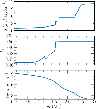
Figure 1: Specific entropy, electron fraction, and mass density profiles as function of stellar mass for the 1D MESA model at the time of mapping into FLASH . The dashed black vertical line denotes the edge of the domain used in the FLASH simulations.

In Figure 1 we show the specific entropy, electron fraction, and mass density profiles as a function of mass coordinate from the MESA model at the point which it is mapped into FLASH . The dashed black line denotes the edge of the domain considered in the FLASH simulations. Overall, the model used in this work has a similar structure to the progenitor used in C15 except for the case of the lower central electron fraction in the core. This difference is partially due to the different network used in C15, a basic 8 isotope network that was automatically extended during evolution compared to our static 21 isotope network used in the MESA model for this work. The input MESA model in C15 also had a slightly smaller initial iron core mass, $1.3$ ${M}_{\odot}$ , than the model considered here.

Figure 2 shows the mass fraction profiles for some of the most abundant isotopes for the input MESA model. The label ‘Iron’ denotes the sum of mass fractions of ^52,54,56Fe isotopes. At the point of mapping the stellar model has an iron core mass of approximately 1.44 $M_{\odot}$. The Si-shell region is located at a specific mass coordinate of $m\approx 1.53-1.68$ ${M}_{\odot}$ while the O-shell region extends from the edge of the Si-shell out to mass coordinate of $m\approx 2.26$ ${M}_{\odot}$ . Figure 3 shows the time evolution of the Brunt-Väisälä frequency (left) and convective velocity speeds as a function of mass coordinate as predicted by MESA for the 1D model evolved from the point at which it is mapped into FLASH until core collapse. The 1D model predicts convective speeds in the O-shell regions with a peak of approximately 100 km s^-1 up to the point of collapse. In the Si-shell region, only the inner most region is convectively active with speeds on the order of those in the O-shell. At a time of $t\approx 200$ s, the innermost Si-shell burning convective region ceases and convective proceeds instead at a further mass coordinate of $m\approx 1.60-1.68$ ${M}_{\odot}$ with speeds increasing to values greater than in the O-shell near collapse at $\approx 160$ km s^-1.

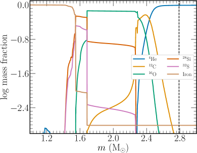
Figure 2: Mass fractions of the most abundant isotopes as a function of stellar mass for the 1D MESA model at time of mapping into FLASH . The label ‘Iron’ denotes the sum of mass fractions of ^52,54,56Fe isotopes. The dashed black vertical line denotes the edge of the domain in FLASH .

2.2 2- and 3D FLASH Stellar Evolution Model

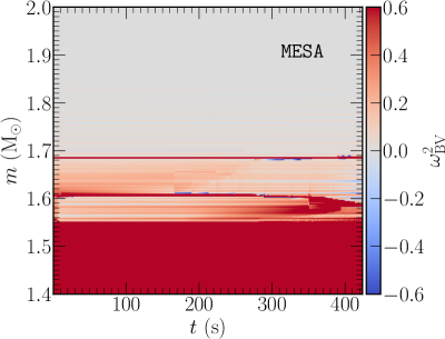
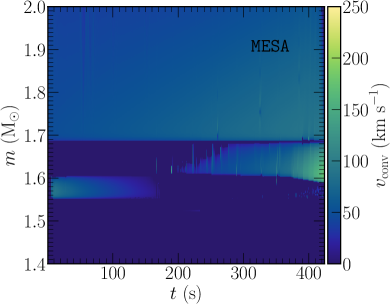
Figure 3: Time evolution of the 1D profile data for the MESA model. The (left) subplot shows the Brunt-Väisälä frequency while the (right) shows the convective velocity speeds according to MLT. The red regions denote regions that are stable against convection while gray and blue regions show regions that are unstable to convection according to MESA.

2.2.1 Overview

We perform a total of multidimensional stellar evolution models at various resolutions and symmetries. All models are evolved using the FLASH simulation framework (Fryxell et al., 2000; Dubey et al., 2009). Similar to Couch et al. (2015), we utilize the “Helmholtz” EoS (Timmes & Swesty, 2000) and the same 21 isotope network but with an improvement to the weak reaction rate used for electron capture onto ⁵⁶Ni. The original network used tabulated rates from Mazurek et al. (1974) while the updated rates were adopted from Langanke & Martínez-Pinedo (2000). The new rates are enhanced by close to a factor of 5-10 alleviating any need to artificially enhance the total electron capture rates in the models presented in this work and are also in agreement with the table values used in MESA .

2.2.2 Hydrodynamics, Gravity, and Domain

The equations of compressible hydrodynamics are solved using FLASH’s directionally unsplit piecewise parabolic method (PPM) (Lee & Deane, 2009) and HLLC Riemann solvers (Toro, 1999) with a Courant factor of 0.8. Self-gravity is solved assuming a spherically symmetric (monopole) gravitational potential approximation (Couch et al., 2013). Our computational domain extends to 10¹⁰ cm from the origin in each dimension for both the 2D and 3D models. Four 2D models are evolved with varying levels of finest grid spacing resolution of 8,16, 24, and 32 km. The 2D models use cylindrical geometry with symmetry about the azimuthal direction. 3D models are evolved: two assuming octant symmetry with two different values of finest grid resolution, 16 and 32 km, and two full $4\pi$ 3D models at 32 km finest grid resolution, . All 3D models use Cartesian coordinates. The models are labeled according to their dimensionality and finest grid spacing, and in the case of 3D according to the use of octant symmetry or not. For example, the 3D 32 km octant model is labelled 3DOct32km for ease of model identification throughout the remainder of this paper. .

All models utilize adaptive mesh refinement (AMR) with up to eight levels of refinement. To give an example of the grid structure for our models we consider the refinement boundaries for the 2D8km and 2D32km models. In the entire Si-shell region has a grid resolution of 32 km with effective angular resolution of $\approx$ 0.9^∘ to 0.5^∘ at the base ( 2000 km) and edge of the shell ( 3500 km), respectively. The grid resolution in the 2D models are representative of the respective 3D models as well. The two finer resolution levels of model are situated within the iron core with the second highest level of refinement at the base of the Si-shell region and down to a radius of 1000 km. . The O-shell region in is at 64 km out to a radius of $\approx$ 6000 km then decreases to 128 km from there to 10,000 km. Within these two regions the effective angular resolution ranges from 0.73^∘ to 0.61^∘ . In the 2D32km, the finest resolution level goes out to a radius of 3500 km, the approximate edge of the Si-shell, giving the model similar resolution in this and the O-shell to that of the 2D8km without the two finer resolution levels within the iron core.

For the 3D octant symmetry planes and the 2D axis plane we use reflecting boundary conditions while the outer boundaries utilize a boundary condition that applies power-law extrapolations of the velocity and density fields to approximate the roughly hydrostatic outer envelope of the stellar interior. The 4$\pi$ 3D models use the same custom boundary condition at all domain edges. To help any transients that occur from mapping we use the approach of Zingale et al. (2002).

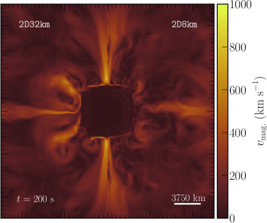
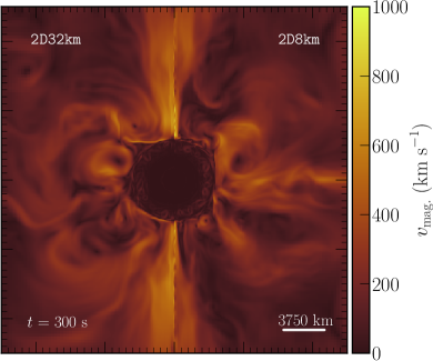
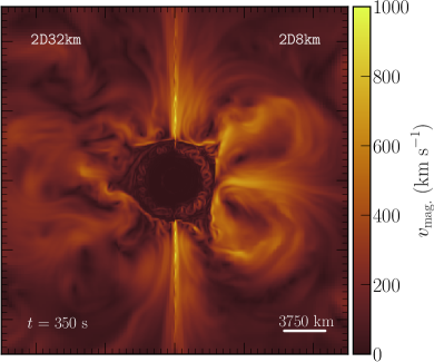
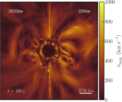
Figure 4: Slices of the the magnitude of the velocity field for the 2D32km (left) and 2D8km model (right) at four different times. At $t=200$ s, both models exhibit a “square” like imprint in the velocity field that is due to the stiff entropy barrier at the edge of the Si-shell region along with increased velocity speeds along the axis. These speeds are due to numerical artifacts common in 2D simulations assuming axisymmetry. The increased velocity along the axis causes outflows in the positive radial direction at the top and bottom of the Si-shell region. Beyond $t=200$ s, both models characterized by large scale cyclones in the O-shell region with convective activity in the Si-shell having slower flow speeds.

2.2.3 Nuclear Burning

During the growth of the iron core, thermal support is removed from the core due to photo-disintegration of iron nuclei that cause the gas to cool. The subsequent contraction of the stellar core causes an increase in the rate of electron captures onto protons therefore decreasing the pressure support contribution from electron degeneracy. This further reduction of pressure support in the core accelerates nuclear burning in the silicon burning shell leading to faster growth of the iron core. In the moments prior to iron core collapse the core moves towards nuclear statistical equilibrium while the neutrino cooling and photo-disintegration rates begin to dominate and lead to a negative specific nuclear energy generation rate, $\epsilon_{\rm{nuc}}$, in the inner core. Within this cooled material, the electron capture rates increase significantly and give rise to a positive specific $\epsilon_{\rm{nuc}}$ and cause the temperature to rise again. Within this region a numerical instability can occur for calculations which employ operator split burning and hydrodynamics (Timmes et al., 2000). In order to avoid this instability from occurring in the models considered here, we place a limiter on the maximum timestep such that any change in the internal energy across all zones in the domain is limited to a maximum of a 1$\%$ per timestep.

The large and opposite specific nuclear energy generation rates within the core can also lead to significant difficulties in solving the nuclear reaction network at a given timestep and lead to significant load imbalance of the computational workload per MPI rank. Zones within the core can take several hundred iterations to obtain a solution while outside of the iron core, a solution is found in a fraction of the time. In order to help circumvent these issues, we employ a moving “inner boundary condition” within the iron core, well below the region of interest for this paper. For all simulations considered here, the profiles of $\rho,Y_{\rm{e}}$, and $P$ in the inner 1000 km of the models are evolved according to the profile from the MESA model at the corresponding time. A 2D table is constructed from the MESA profile data from the point of mapping to FLASH ($\approx 424$ s) until iron core collapse. Four point Lagrange linear interpolation is then performed in time and radius to ensure accurate values are mapped for the FLASH models, which take on the order of 100 timesteps for every MESA timestep. This mapping effectively provides a time-dependent inner boundary condition that ensures the model follows the central evolution of the MESA model while still allowing us to capture the pertinent multi-D hydrodynamic behavior with FLASH .

For all models, we simulate $\approx$ 424 s of evolution prior to collapse capturing Si- and O-shell burning up to gravitational instability and iron core collapse. The full $4\pi$ 3D models had an approximate total of 46M zones, took $\approx$ 0.6 M core hours on the laconia compute cluster at Michigan State University. All the multidimensional CCSN progenitor models considered in this work are available publicly athttps://doi.org/10.5281/zenodo.3976246 (catalog 10.5281/zenodo.3976246).

3 Multi-Dimensional Evolution to Iron Core-Collapse

3.1 Results from 2D Simulations

We evolve a total of four 2D simulations at 8,16, 24, and 32 km finest grid spacing resolution. In the following subsection we consider the global properties of all of the 2D models, compare the lowest and highest resolution model, and consider in detail the convective properties of the highest resolution 2D model.

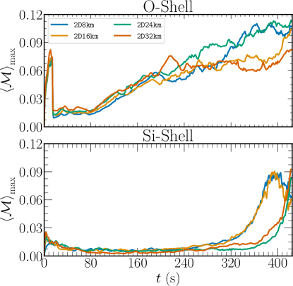
Figure 5: Time evolution of the maximum angle-averaged Mach number within the Si- and O-shell for all 2D models.

The structure of the flow at large scale within the shell burning regions can have a significant impact on the CCSN explosion mechanism. Perturbations within these region can be amplified during collapse of the iron core and aid in the development of turbulence during explosion (Lai & Goldreich, 2000; Couch & Ott, 2013, 2015). In Figure 4 we show slices of the magnitude of the velocity field for the 2D32km (left ) and 2D8km models (right ) at four different times. At early times, we see convection developing in a similar matter for both the 8 km and 32 km models. Both models exhibit a “square” like imprint in the velocity field that is due to the stiff entropy barrier at the edge of the Si-shell region interacting with the Cartesian-like 2D axisymmetric grid. $t=200$ s both models characterized by large scale cyclones in the O-shell region At late times, beyond $t=350$ s, the 8 km model appears to reach flow speeds in the Si-shell that are on the order of those observed in the O-shell. In the O-shell, the scale of the convection increases as cyclones on the order of $\approx$ 4000 km dominate the flow with the scale of convection within the Si-shell region being restricted by the width of the shell. Seconds prior to collapse, the 32 km model reaches Si-shell convective speeds that agree with the 8 km model.

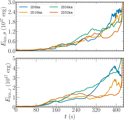
Figure 6: Time evolution of the radial and non-radial kinetic energy for the four 2D models.

To begin our assessment of the convective properties of the models, we compute the angle-averaged maximum Mach number, defined as,

$$\left<\mathcal{M}\right>=\left<\frac{\left|\bf{v}\right|}{c_{\rm{s}}}\right>~{},$$ (1)

where $\left|\textbf{v}\right|$ is the local magnitude of the velocity field and $c_{\rm{s}}$ the local sound speed, and the averaging is performed over solid angle. We also compute the Mach number within the Si-shell and within the O-shell to characterize their behavior independently. The shell region for silicon-28 is defined as the region where $X(^{28}\rm{Si})>0.2$ and $X(^{16}\rm{O})<0.2$ and for oxygen-16 $X(^{16}\rm{O})>0.2$ and $X(^{28}\rm{Si})<0.2$.

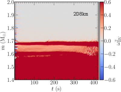
Figure 7: Same as in Figure 3 but for the 2D8km FLASH simulation. The slightly negative values of $\omega^{2}_{\rm{BV}}$ denoted by the gray/light blue regions represent regions unstable to convection.

In Figure 5 we show the time evolution of the maximum angle-averaged Mach number for all 2D models. The maximum Mach number reported at the start of the simulation reflects the initial transient as it traverses the domain. Beyond $t\approx 15$ s, the transient has either traversed the shell region or been sufficiently damped that the Mach numbers reflect the convective properties of the shells and not the initial radial wave. The Si-shell appears to reach a quasi-steady state in the first $\approx$ 80 seconds, this is seen by all models reaching a characteristic Mach number within the shell. In the O-shell, the Mach number remains relatively flat although larger than the approximate mean in the Si-shell, this suggests little to no convective activity in the O-shell during this time. To make an estimate of the time at which these two regions would be expected to reach a quasi-steady convective state, we can estimate a convective turnover timescale for each region. The Si-shell spans a radius of approximately 800 km with convective speeds of $v_{\rm{Si-shell}}\approx 80$ km s^-1 at early times. Using this, we can estimate an approximate convective turnover time within the Si- shell of $\tau_{{\rm{Si}}}\approx 2r_{\rm{Si}}/v_{\rm{Si}}\approx 20$ seconds. This value suggests that after the transient has traversed the Si-shell region, a total of approximately three turnover timescales elapse before the region reaches a quasi-steady state represented by an average Mach number oscillating on the approximate timescale of the turnover time. A similar estimate can be made to the O-shell where we determine a turnover time of $\tau_{\rm{O}}\approx$ 100 seconds. This value suggests that the lack of change in Mach number for the O-shell is due to the fact that the region has not yet reached a quasi-steady convective state.

By the end of the simulation, the models span a range of Mach numbers of $\approx 0.08-0.12$.

The late time behavior of the Si-shell region of the two highest resolution models can be attributed to an expansion of the width of the convective Si-shell region observed in the last slice of Figure 4 . the two highest resolution models, the convective velocity speeds reach enough to overcome the barrier between the convective and non-convective silicon shell regions causing them to merge. After this merging of these two regions, the entire region becomes fully convective. However, due to the expansion of the width of the Si-shell region after merging, the burning within this region occurs at lower density. Because the local sound speed goes as $c_{\rm{s}}\propto\rho^{-1/2}$, a decrease in density leads to an increase in the sound speed therefore decreasing the local maximum Mach number. The two lower resolution models do not experience this merging of the two regions until moments before collapse when the flow speeds are large enough $\approx$ 150 km s^-1 to merge.

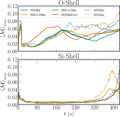
Figure 8: Same as in Figure 5 but for all the 3D models for the duration of the simulation.

In Figure 6 we show the time evolution of the total kinetic energy in the radial and non-radial components for the 2D FLASH models. When considering the non-radial kinetic energy components for the four models we see that the peak value of the energy at collapse increases with an increase in model resolution with the highest resolution model showing a peak value of $E_{\rm{kin.},\theta}\approx 2.5\times 10^{47}$ erg at collapse. The radial kinetic energy shows further evidence for the expansion of the Si-shell region in the two highest resolution models with the energies showing local maxima around $t\approx$ 390 s followed by a steady decline for the duration of the simulation. This transition time is also reflected in the non-radial kinetic energy where one can notice a slight increase in the energy from $t\approx 390$ s to collapse.

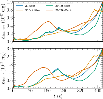
Figure 9: Same as in Figure 6 but for the four 3D models.

In Figure 7 (left) we show the time evolution of the Brunt-Väisälä frequency for the assuming the Ledoux criterion for convection which states that a region is stable against convection if

$$\nabla_{\rm{rad.}}<\nabla_{\rm{ad.}}-\frac{\chi_{\mu}}{\chi_{T}}\nabla_{\mu}~{}.$$ (2)

Under this criterion, we can compute the Brunt-Väisälä frequency for the FLASH simulations as

$$\omega^{2}_{\rm{BV}}=g\left(\frac{1}{\rho}\frac{\partial{\rho}}{\partial{r}}-\frac{1}{\rho c^{2}_{\rm{s}}}\frac{\partial{P}}{\partial{r}}~{}\right)~{},$$ (3)

where $g$ is the local gravitational acceleration, $\rho$ the mass density, $c_{\rm{s}}$ the adiabatic sound speed, and $P$ the pressure. This form of the Brunt-Väisälä frequency equation is equivalent to forms that explicitly include the entropy and electron fraction gradients (Müller et al., 2016). For each timestep for which these 2D data are available, we compute angle average profiles as a function of radius before using Equation 3 to compute the frequency. Using this convention a positive value implies a region stable against convection.

In Figure 7 we also show the time evolution of the convective velocity (right), here defined as $v_{\rm{conv}}=\sqrt{|\textbf{v}|^{2}-v^{2}_{\rm{rad.}}}$, as a function of time for the same model. The base of the O-shell region is shown at an approximate mass coordinate of 1.7 ${M}_{\odot}$ . Within the O-shell, the convective velocity reach speeds of nearly 500 km s^-1 as the model approaches iron core collapse. Prior to this, the model shows values on the order of 50-100 km s^-1 in the Si-shell and 200-400 km s^-1 in the O-shell. The expansion of the convective Si-shell region due to the merging is observed as well in the convective velocity, again around $t\approx 390$ s, the same time at which the velocity begins to reach values observed in the O-shell for this model. In comparing to Figure 3, the FLASH model predicts two initial inner and outer convectively active regions that eventually merge into one larger region near collapse. On the other hand, the MESA model predicts a transition of the location of the convective region followed by late time expansion of this region near collapse. Despite these somewhat different evolutionary pathways both models agree in their qualitative description of the location of the convective regions near collapse. The major difference between the two models are the magnitude of the convective velocities predicted by MESA /MLT.

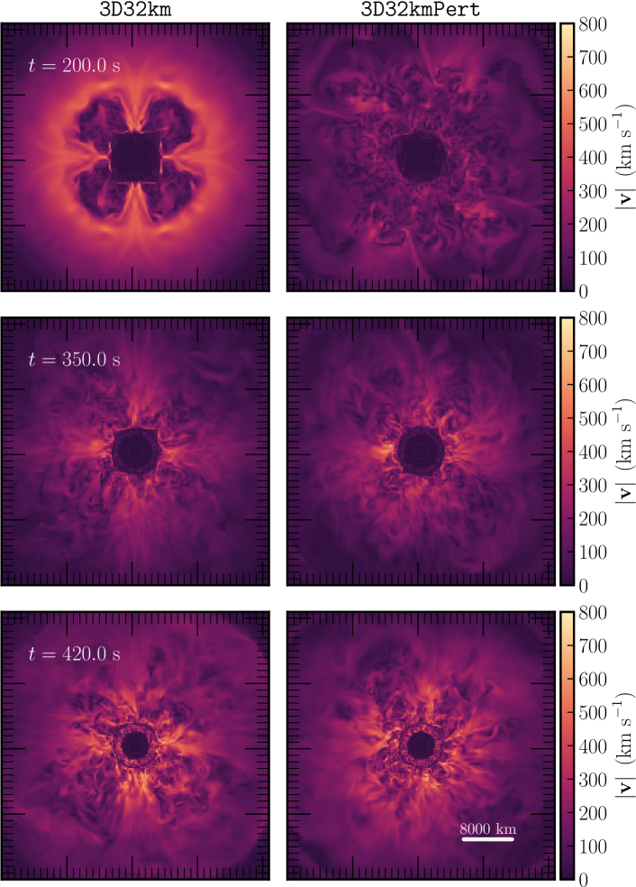
Figure 10: Slices of the the magnitude of the velocity field for the 3D32km (left) and 3D32kmPert (right) models at $t=$ 200 s, 350 s, and 420 s in the $x-y$ plane.

3.2 Results from 3D Simulations

We perform a total of 3D stellar models: two models in octant symmetry at 16 and 32 km finest grid spacing and full 4$\pi$ models at 32 km finest resolution . In this subsection, we will consider the global properties of all 3D models, describe the perturbed 4$\pi$ 32 km in detail, and, lastly, consider the impact of octant symmetry and resolution.

In Figure 8 we show the time evolution of the maximum Mach number in the Si- and O-shell at each timestep for all 3D models. Contrary to the trend seen in Figure 5 for the O-shell one can observe a periodic nature in the Mach number values that follows our estimate for the convective turnover timescales from Section 3.1. Similar to the comparable 2D case (see Figure 6), the 3DOct16km model appears to reach a peak Mach number in the Si-shell at around $t\approx 390$ s before a steady decline as the model approaches collapse, this behavior is also attributed to expansion of the Si-shell after the merging of the convective and non-convective regions. This result suggests that the merger is independent of geometry and dimensionality but instead depends on the resolution of the inner core region.

Figure 9 shows the time evolution of the radial and non-radial kinetic energy for the 3D models. In general, the 32 km resolution models behave similarly with the 4$\pi$ models having larger kinetic energy values than the octant model beyond $t\approx 280$ s. The 16 km octant model has larger kinetic energy values than both models at late times while also reaching a local peak value approximately 30 s before collapse. Prior to about 200 s, the bulk of the energy in the radial direction for the two unperturbed 32 km models is due to an the initial transient that traverses the domain at the start of the simulation and leaves the domain at $t\approx$ 60 s. The 16 km model experiences a less significant initial transient and therefore undergoes less initial expansion/contraction as the model readjusts to a new equilibrium.

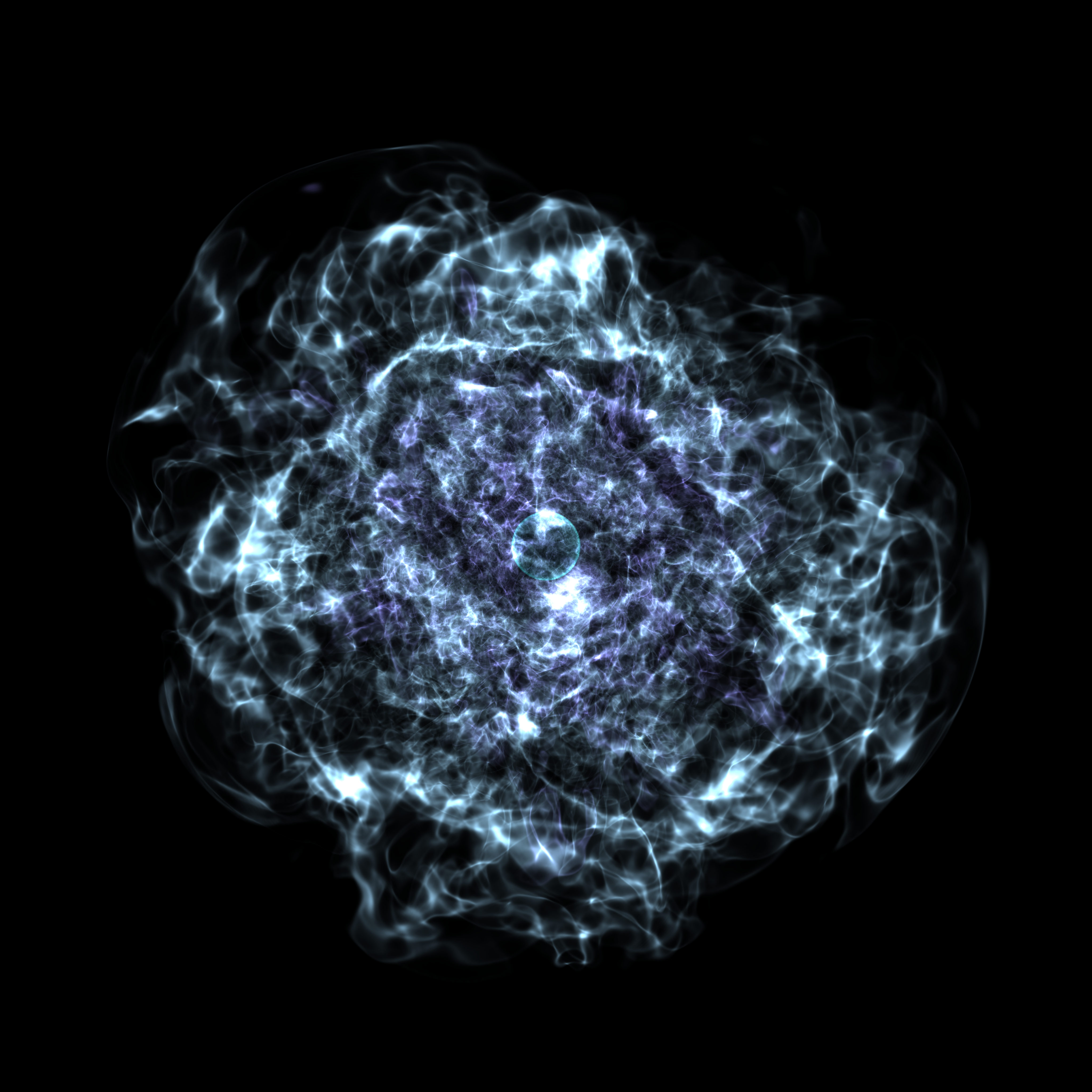
Figure 11: 3D volume rendering of the magnitude of the velocity field for the 4$\pi$ 3D32kmPert model at a time $\approx$ 2 seconds before iron core collapse. The teal contour denotes the edge of the iron core defined to be the radius at which $s\approx$ 4 $k_{\rm{KB}}$ / baryon. At this time, the iron core spans a radius of $r\approx 1982$ km. The light purple plumes represent O-shell burning convection speeds following a Guassian with a peak at $\left|\bf{v}\right|\approx 300$ while the light blue plumes $\left|\bf{v}\right|\approx 100$ This image was made using yt and the color map library cmocean.

The evolution of the magnitude of the velocity field for models 3D32km (left) and 3D32kmPert (right) is compared in Figure 10.

In Figure 11 we show a 3D volume rendering of the magnitude of the velocity field for the 3D32kmPert model at $t\approx 423$ s. The approximate location of the edge of the iron core (shown in teal) is taken to be an isocontour surface at a radius where $s\approx$ 4 $k_{\rm{KB}}$ / baryon. At this time, the iron core has a radius of $r\approx 1982$ km. The light purple plumes show the fast moving convective motions in the O-shell region depicted by a Guassian transfer function with a peak at $\left|\bf{v}\right|\approx 300$ . The slower moving, larger scale motions are shown using a similar transfer function with a peak at $\left|\bf{v}\right|\approx 100$ in light blue.

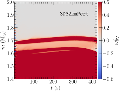
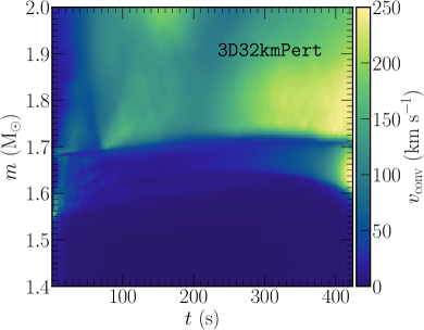
Figure 12: Same as in Figure 3 but for the 3D32kmPert FLASH simulation.

Similar to the analysis done for the MESA model and the 2D FLASH models, in Figure 12 we show the Brunt-Väisälä frequency (left) and convective velocity (right) as a function of time for the 3D32kmPert FLASH model. Unlike the 2D8km, this model does not experience the merging of the two Si regions until a few seconds prior to collapse leading to a similar fully convective Si-shell at the end of the simulation. Another notable feature of this model is the slight expansion and then contraction of different regions of the model. For example, the base of the O-shell region begins at a mass coordinate of $m\approx 1.68$ ${M}_{\odot}$ in all models but appears to expand outward to a coordinate of $m\approx 1.72$ ${M}_{\odot}$ for the 3D32km model at about $t\approx 200$ s. This expansion is not observed in the 2D8km model but is partially due to the initial transient at the beginning of the simulation, . The impact of this effect on our main results will be considered in Section 3.2.2.

3.2.1 Characterizing the convection in the 3d32kmPert model

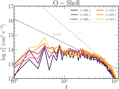
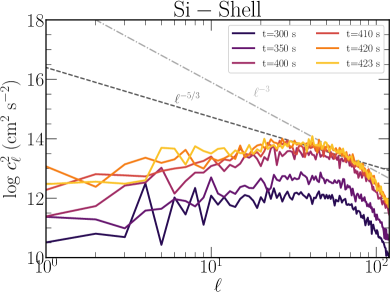
Figure 13:

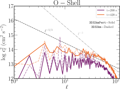
Figure 14: Same as in Figure 13 but only considering the O-shell region for the 3D32km and 3D32kmPert models at two different times.

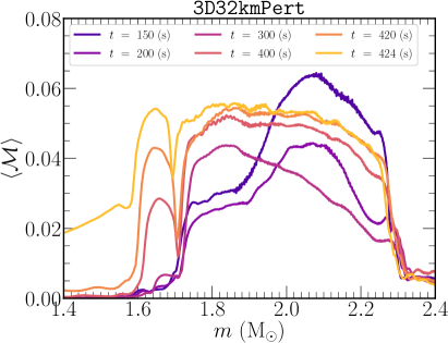
Figure 15: The profile of the angle averaged Mach number as a function of mass coordinate at six different times for the 3D32kmPert stellar model. At $t=424$ s the average Mach number reaches $\left<\mathcal{M}\right>\approx 0.06$ in the Si-shell and at the base of the O-shell.

To characterize the scales of the convective eddies and the overall evolution of the strength of convection throughout the duration of the simulations we

$$c^{2}_{\ell}=\sum\limits^{\ell}_{m=-\ell}\left|\int Y^{m}_{\ell}(\theta,\phi)\left|\textbf{v}\right|^{\prime}(r_{\rm{Shell}},\theta,\phi)d\Omega\right|^{2}~{},$$ (4)

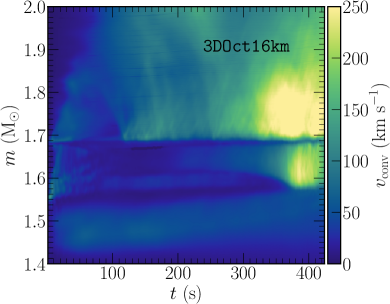
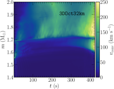
Figure 16: The evolution of the convection velocity profiles for the 16km and 32km 3D octant models.

In Figure 15 we show the angle-averaged Mach number profile as a function of mass coordinate for the 3D32kmPert model at six times. The Si-shell region is situated at a mass coordinate of approximately 1.6 to 1.7 ${M}_{\odot}$ . The evolution of the Mach number in this region is further representative of the power spectra shown in Figure 13. For the majority of the simulation, the Mach numbers in this region are on the order of $\left<\mathcal{M}\right>\lesssim 0.01$. Only at times beyond $t\approx 300$ s do they increase significantly reaching values of $\left<\mathcal{M}\right>\approx 0.06$ prior to collapse. In the O-shell region, at mass coordinates of $m\approx 1.7-2.3\ M_{\odot}$, the Mach numbers reach values of about $\left<\mathcal{M}\right>\approx 0.06$ as early as $t\approx 150$. At late times, the O-shell region approaches Mach numbers of $\left<\mathcal{M}\right>\approx 0.06$ near collapse.

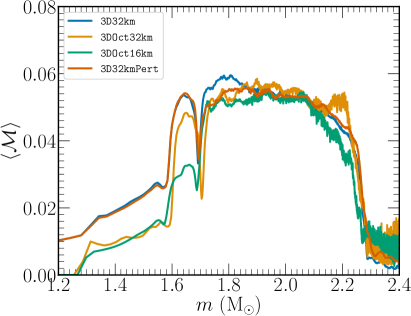
Figure 17: The Mach number profiles as a function of mass coordinate for the four 3D models .

3.2.2 Effect of Spatial Resolution and Octant Symmetry

To assess the impact of spatial resolution and octant symmetry we compare the results of the two $4\pi$ 3D32km simulations with the two 3D octant models. In Figure 16 we show the time evolution of the convective velocity profiles for the 3DOct16km and 3DOct32km models. We can observe the same expansion of the O-shell region in the 32 km octant model as with the full 4$\pi$ models. In contrast, the 16 km octant model does not appear to undergo this contraction and the base of the O-shell stays at a steady mass coordinate for the duration of the simulation. Moreover, the 16 km model reaches larger convective velocities in the Si- and O-shell regions at $t\approx$ 350 s. This time corresponds to the same time at which we observe a peak in the Mach numbers in Figure 8 and is due to the merging of the convective and non-convective regions. These results suggest that due to the stability of the O-shell in the 16 km model, the model follows a slightly different evolution than that of the 32 km octant and 4$\pi$ models characterized by larger convective velocity speeds that facilitate merging of convective and non-convective regions in the Si-shell. Moreover, it suggests that these differences are attributed more to the finest grid spacing of the inner core region and less dependent on the symmetry imposed for the octant models. Despite the differences found in the evolution of the Si-shell region between these two models, the O-shell region appears less impacted by the difference in resolution and arrive at similar qualitative properties among the 3D models.

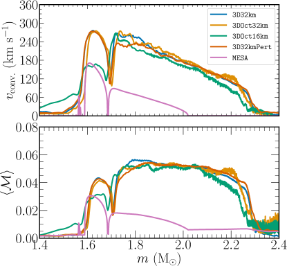
Figure 18: The convective velocity (top) and Mach number (bottom) for the 1D MESA model and angle-averaged profiles of the four 3D models at the $t\approx 420$ s.

We can further determine the effect that resolution and symmetry has on our results by considering some keys aspects of our 3D stellar models at collapse that have significant implications for simulations of CCSNe. Couch & Ott (2013) considered the effect of ashpericities of imposed perturbations in the -shell regions characterized by the magnitude of the Mach number. They found large Mach number perturbations can result in enhanced strength of turbulent convection in the CCSN mechanism, aiding explosion. In Figure 17, we plot the profiles of the Mach number at the start of collapse, , for the 3D models. In general, we see that the estimates of the Mach number in the O-shell region between $\approx$1.7-2.3 ${M}_{\odot}$ across all models, the at the base of the O-shell in the $4\pi$ model, showing an $\approx 8\%$ larger value. The main difference is observed in the Si-shell region where the Mach number is approximately larger in the 32 km models, which agree with each other to $\approx$ 10%.

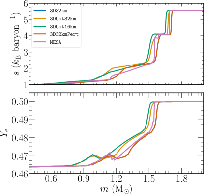
Figure 19: The specific entropy (top) and specific electron fraction (bottom) for the 1D MESA model and angle-averaged profiles of the four 3D models at the $t\approx 420$ s.

When comparing the 32 km octant and $4\pi$ models it is likely the case that the convective speeds are able to reach larger values as large scale flow is not suppressed at the symmetry planes. This is supported further by the larger non-radial kinetic energy in the $4\pi$ models as seen in Figure 9.

Another important diagnostic of the presupernova structure is the compactness parameter (O’Connor & Ott, 2011),

$$\xi_{m}=\left.\frac{m/M_{\odot}}{R(M_{\rm{bary}}=m)/1000\textup{ km}}\right|_{t=t_{\rm{cc}}},$$ (5)

where a value of 2.5 ${M}_{\odot}$ is typically chosen for evaluation at the start of core collapse. The value of this quantity in the progenitor star has been shown to be highly non-monotonic with ZAMS mass but gives some insight to the ensuing dynamics of the CCSN mechanism for a given progenitor (Sukhbold et al., 2018; Couch et al., 2019). We can compute this quantity for our three 3D models to determine how much variation exists due to the effects of resolution and symmetry. Using Equation (5) for the three 3D models at a time $t=424$ s, moments before collapse. We find values of $\xi_{m=2.5M_{\odot}}=$ 0.0473, 0.0474, 0.0331, and 0.0359, for the 3D32kmPert, 3D32km, 3DOct16km, and 3DOct32km models respectively. These values suggest that the imposed octant symmetry can under estimate the compactness of the stellar model at collapse by $\approx 25\%$ while the differences in grid resolution but assuming octant symmetry can result in a difference of less than $\approx 10\%$. The compactness value at approximately the equivalent time for the MESA model was $\xi_{m=2.5M_{\odot}}=0.0492$ agreeing with the 3D32km to within less than 4%. Our values are approximately a factor of two less than those found in Sukhbold et al. (2018) and a factor of four less than those in Sukhbold & Woosley (2014) .

3.3 Comparison between the 1- and 3D Simulations

In this subsection we compare the angle-averaged properties of the of the 1D MESA model and the 3D models at a time near iron core collapse. In Figure 18 we show the convective velocity (top) and Mach number (bottom) for these models at $t\approx 420$ s. Considering first the O-shell region, situated at a mass coordinate between $m\approx 1.7-2.3$ ${M}_{\odot}$ , the convective velocity speeds of the 3D models agree quite well in shape and magnitude. This is with exception to the 3DOct16km model for which the velocities in this region are $\approx$ 5-10 km s^-1 slower. In this region, the 1D MESA model matches the shape of the convective velocity profile somewhat well but predicts a region with considerable convective activity that is smaller in extent, ranging only from $m\approx 1.7-2.0$ ${M}_{\odot}$ . Additionally, the magnitude of the speeds in this region according to MLT are significantly less, $\approx 4-5$ times less, than the values found in our 3D models. The Si-shell region is situated at a mass coordinate of $m\approx 1.55-1.7$ ${M}_{\odot}$ . The convective speeds in the 3D 32 km models agree well within this region while the 3DOct16km model shows a lower speed of $v_{\rm{conv.}}\approx 160$ km s^-1 owing to the merging of the convectively burning and non-convectively burning regions discussed in Section 3.2. The 1D MESA model agrees with 3DOct16km remarkably well in the shape and magnitude of the convective velocity speeds in this region with only slight differences at the outer edge of the Si-shell region being steeper in the 3D model. These trends follow a similar behavior when looking at the Mach number profiles. The MESA model agrees well in shape and magnitude with the 3DOct16km model but significantly underestimates the values in the O-shell region.

We consider the core properties in Figure 19 where we show the specific entropy (top) and electron fraction (bottom) for the same models considered in Figure 18. Note that owing to the “inner boundary condition” used for the core, the specific electron fraction for all the models up to a mass coordinate of $m\approx 0.8$ ${M}_{\odot}$ should be the same value. All models follow a similar specific entropy profile with only minor differences in mass of the iron core, the mass coordinate where $s\approx 4\ k_{\rm{B}}$ baryon^-1. Qualitatively, the specific entropy and electron fraction profiles for the 3D simulations are smoother than those of the MESA model.

4 Summary and Discussion

We have investigated the long term, multidimensional, hydrodynamical evolution of a 15 ${M}_{\odot}$ star for the final seven minutes of Si- and O- shell burning prior to and up to the point of iron core collapse. Using the FLASH simulation framework we evolved eight stellar models at varying resolution, dimensions, and symmetries to characterize the nature of the convective properties of the stellar models and their implications for CCSN explosions.

We find that in general the angle averaged properties of the multidimensional models with predictions made by MESA . The largest differences observed were found when comparing the convective velocities in the O-shell region to those in the MESA model. . Our 2D models showed a convectively active Si-shell region with peak velocities of approximately 500 km s^-1 near collapse and Mach numbers of $\approx$ 0.1 near collapse. Within the O-shell region the 2D models show slightly slower convective speeds of $\approx$ 400 km s^-1 and Mach numbers of 0.8-0.12 depending on the resolution of the simulation. The 3D models show velocities and Mach numbers lower than this in all cases. The 4$\pi$ 3D models had convective velocities of $\approx$ 240-260 km s^-1 in the Si- and O- shell moments prior to collapse with Mach values of 0.06.

To characterize the behavior of the convection of the 4$\pi$ 3D , we computed power spectra of the Si- and O-shell regions by at different times throughout the simulation.

However, despite the differences between these evolutionary paths in the Si-shell, the results of the O-shell region appear largely unaffected by resolution or geometry, resulting in quantitatively similar properties near collapse in all of the 3D models. When comparing the 3D models for different resolutions and symmetries we also found that the Mach number profiles in the O-shell region agreed across all models with only a slight difference shown in the 4$\pi$ where larger Mach numbers ($\approx 8\%$) are found at the base of the O-shell. The Si-shell region Mach number profiles showed that the 3DOct16km model has a smaller value of $\approx 0.03$ while the 3DOct32km reached a value approximately twice of that. This difference is again linked to the merging of the convective and non-convective regions in the 16 km models. Another important diagnostic linking the presupernova structure to the dynamics of the CCSN mechanism is the compactness parameter. When comparing values of this parameter,

In C15, they investigated the final three minutes of Si-shell burning in a 15${M}_{\odot}$ star evolved assuming octant symmetry and a reaction network that included enhanced electron capture rates. They found that convective speeds in the silicon shell reach values of 80-140 km s^-1 near collapse. These values are approximately a factor of smaller than what we find in all of our 3D simulations and a factor of four smaller than the results suggested by our 2D models. A major cause of these differences can likely be attributed to the length of their simulation. In all our multidimensional models considered here the convective velocity speeds did not increase considerably until about five minutes into the simulation. Measuring the turbulent kinetic energy power spectrum for their model they found the bulk of the energy residing at small $l$ values (large scales), at $l\approx 4$ due to the imposed octant symmetry. They also found significant power at an $l\approx 10$ value for the Si-shell region near collapse.

Müller et al. (2016) investigated the last minutes of O-shell burning in a 18 ${M}_{\odot}$ star. They evolved the model for $\approx$ five minutes using a contracting inner boundary condition situated at the base of the O-shell mapped to follow the mass trajectory from the initial Kepler model. In their simulation of O-shell burning they find transverse velocity speeds that reach values of $\approx$ 250 km s^-1 approximately a minute prior to collapse. These values are slightly larger by about 50-100 km s^-1 than the values we find in all of our 3D models at a similar epoch. At the onset of collapse, they observe peak Mach numbers in the O-shell of $\left<\mathcal{M}\right>\approx 0.1$ where we find a value of $\sim$0.06. They compute the power spectrum for the radial velocity component into spherical harmonics to characterize the scale of the convection. At the early times, $t=90.9$ s they find a similar characteristic scale at $l\approx 4$ where the bulk of the power resides. As the simulation evolves the bulk of the power in their model shifts to larger scales at $l\approx 2-4$.

Recently, Yadav et al. (2020) presented a 4$\pi$ 3D simulation of O-/Ne-shell burning using a similar method as presented in Müller et al. (2016). The simulation was evolved for 420 s and captured the merging of a large scale O-Ne shell merger leading to significant deviations from the properties predicted by the 1D initial model. In this work, they found at $t\approx 250$ s, the barrier separating the O- and Ne-shells disappears due to an increase in entropy in the O-shell leading to the merging of the two convective regions. The merger leads to large scale density fluctuations characterized by $l\approx 1-2$ modes within the merged shell. After the merger they observe velocity fluctuations on the order of 800 km s^-1 that increase to as large at 1600 km s^-1 near collapse. At collapse they observe Mach numbers of $\approx 0.13$ in the O/Ne mixed region. These values both suggest that the merger can lead to significantly larger deviations from spherical symmetry than as suggested by the model presented in this work and other simulations of quasi-steady state convection prior to core collapse. Despite the merging of the two unique convective regions in the Si-shell observed in most of our models, we do not observe merging of different burning shell regions in any of our models.

High resolution, long term, 4$\pi$ 3D simulations of CCSN progenitors can provide accurate initial conditions for simulations of CCSNe. An accurate representation of the state of the progenitor prior to collapse can have a favorable impact on the delayed neutrino-driven explosion mechanism and has important implications for the predictions of key observables from CCSN simulations. In addition to fully 3D convection motions, most massive stars are also rotating differentially in their cores. In the presence of weak seed magnetic fields, this rotation can facilitate a large scale dynamo that can have an impact on the progenitor evolution and the explosion mechanism. As such, a next step in increasing the physics fidelity of supernova progenitor models would be to consider the impact of a rotating and magnetic progenitor on the observed scale and magnitude of perturbations within the late time burning shell regions. The direct link between multidimensional rotating and magnetic CCSN progenitors and the CCSN mechanism is an important question and is the direction of future work.

References

- Arnett (1994) Arnett, D. 1994, ApJ, 427, 932, doi: 10.1086/174199
- Arnett et al. (2009) Arnett, D., Meakin, C., & Young, P. A. 2009, ApJ, 690, 1715. https://arxiv.org/abs/0809.1625
- Arnett & Meakin (2011) Arnett, W. D., & Meakin, C. 2011, ApJ, 733, 78, doi: 10.1088/0004-637X/733/2/78
- Böhm-Vitense (1958) Böhm-Vitense, E. 1958, ZAp, 46, 108
- Botticella et al. (2012) Botticella, M. T., Smartt, S. J., Kennicutt, R. C., et al. 2012, A&A, 537, A132, doi: 10.1051/0004-6361/201117343
- Côté et al. (2017) Côté, B., O’Shea, B. W., Ritter, C., Herwig, F., & Venn, K. A. 2017, ApJ, 835, 128, doi: 10.3847/1538-4357/835/2/128
- Couch et al. (2015) Couch, S. M., Chatzopoulos, E., Arnett, W. D., & Timmes, F. X. 2015, ApJ, 808, L21, doi: 10.1088/2041-8205/808/1/L21
- Couch et al. (2013) Couch, S. M., Graziani, C., & Flocke, N. 2013, ApJ, 778, 181, doi: 10.1088/0004-637X/778/2/181
- Couch & O’Connor (2014) Couch, S. M., & O’Connor, E. P. 2014, ApJ, 785, 123, doi: 10.1088/0004-637X/785/2/123
- Couch & Ott (2013) Couch, S. M., & Ott, C. D. 2013, ApJ, 778, L7, doi: 10.1088/2041-8205/778/1/L7
- Couch & Ott (2015) —. 2015, ApJ, 799, 5, doi: 10.1088/0004-637X/799/1/5
- Couch et al. (2019) Couch, S. M., Warren, M. L., & O’Connor, E. P. 2019, arXiv e-prints, arXiv:1902.01340. https://arxiv.org/abs/1902.01340
- Cox & Giuli (1968) Cox, J. P., & Giuli, R. T. 1968, Principles of Stellar Structure (New York: Gordon & Breach)
- Dubey et al. (2009) Dubey, A., Antypas, K., Ganapathy, M. K., et al. 2009, Parallel Computing, 35, 512 , doi: https://doi.org/10.1016/j.parco.2009.08.001
- Farmer et al. (2016) Farmer, R., Fields, C. E., Petermann, I., et al. 2016, ApJS, 227, 22, doi: 10.3847/1538-4365/227/2/22
- Farmer et al. (2015) Farmer, R., Fields, C. E., & Timmes, F. X. 2015, ApJ, 807, 184, doi: 10.1088/0004-637X/807/2/184
- Fields et al. (2018) Fields, C. E., Timmes, F. X., Farmer, R., et al. 2018, ApJS, 234, 19, doi: 10.3847/1538-4365/aaa29b
- Fryxell et al. (2000) Fryxell, B., Olson, K., Ricker, P., et al. 2000, ApJS, 131, 273, doi: 10.1086/317361
- Glas et al. (2019) Glas, R., Just, O., Janka, H. T., & Obergaulinger, M. 2019, ApJ, 873, 45
- Hanke et al. (2013) Hanke, F., Müller, B., Wongwathanarat, A., Marek, A., & Janka, H.-T. 2013, ApJ, 770, 66
- Heger et al. (2000) Heger, A., Langer, N., & Woosley, S. E. 2000, ApJ, 528, 368
- Heger & Woosley (2010) Heger, A., & Woosley, S. E. 2010, ApJ, 724, 341, doi: 10.1088/0004-637X/724/1/341
- Hopkins et al. (2011) Hopkins, P. F., Quataert, E., & Murray, N. 2011, MNRAS, 417, 950, doi: 10.1111/j.1365-2966.2011.19306.x
- Hunter (2007) Hunter, J. D. 2007, Computing In Science & Engineering, 9, 90
- Janka (2012) Janka, H.-T. 2012, Annual Review of Nuclear and Particle Science, 62, 407, doi: 10.1146/annurev-nucl-102711-094901
- Jones et al. (2016) Jones, S., Andrassy, R., Sandalski, S., et al. 2016, ArXiv e-prints. https://arxiv.org/abs/1605.03766
- Kraichnan (1967) Kraichnan, R. H. 1967, Physics of Fluids, 10, 1417
- Lai & Goldreich (2000) Lai, D., & Goldreich, P. 2000, ApJ, 535, 402
- Langanke & Martínez-Pinedo (2000) Langanke, K., & Martínez-Pinedo, G. 2000, Nuclear Physics A, 673, 481, doi: 10.1016/S0375-9474(00)00131-7
- Lee & Deane (2009) Lee, D., & Deane, A. E. 2009, Journal of Computational Physics, 228, 952 , doi: https://doi.org/10.1016/j.jcp.2008.08.026
- Lentz et al. (2015) Lentz, E. J., Bruenn, S. W., Hix, W. R., et al. 2015, ApJ, 807, L31
- Mabanta & Murphy (2018) Mabanta, Q. A., & Murphy, J. W. 2018, ApJ, 856, 22, doi: 10.3847/1538-4357/aaaec7
- Mazurek et al. (1974) Mazurek, T. J., Truran, J. W., & Cameron, A. G. W. 1974, Ap&SS, 27, 261, doi: 10.1007/BF00643877
- Meakin & Arnett (2007) Meakin, C. A., & Arnett, D. 2007, ApJ, 665, 690, doi: 10.1086/519372
- Muller & Janka (2015) Muller, B., & Janka, H.-T. 2015, Monthly Notices of the Royal Astronomical Society, 448, 2141, doi: 10.1093/mnras/stv101
- Müller et al. (2017) Müller, B., Melson, T., Heger, A., & Janka, H.-T. 2017, MNRAS, 472, 491
- Müller et al. (2016) Müller, B., Viallet, M., Heger, A., & Janka, H.-T. 2016, ArXiv e-prints. https://arxiv.org/abs/1605.01393
- Murphy et al. (2013) Murphy, J. W., Dolence, J. C., & Burrows, A. 2013, ApJ, 771, 52
- Nagakura et al. (2019) Nagakura, H., Burrows, A., Radice, D., & Vartanyan, D. 2019, arXiv e-prints. https://arxiv.org/abs/1905.03786
- O’Connor & Ott (2011) O’Connor, E., & Ott, C. D. 2011, ApJ, 730, 70, doi: 10.1088/0004-637X/730/2/70
- O’Connor & Couch (2018a) O’Connor, E. P., & Couch, S. M. 2018a, ApJ, 865, 81, doi: 10.3847/1538-4357/aadcf7
- O’Connor & Couch (2018b) —. 2018b, ApJ, 854, 63, doi: 10.3847/1538-4357/aaa893
- Özel et al. (2012) Özel, F., Psaltis, D., Narayan, R., & Santos Villarreal, A. 2012, ApJ, 757, 55, doi: 10.1088/0004-637X/757/1/55
- Paxton et al. (2011) Paxton, B., Bildsten, L., Dotter, A., et al. 2011, ApJS, 192, 3, doi: 10.1088/0067-0049/192/1/3
- Paxton et al. (2013) Paxton, B., Cantiello, M., Arras, P., et al. 2013, ApJS, 208, 4, doi: 10.1088/0067-0049/208/1/4
- Paxton et al. (2015) Paxton, B., Marchant, P., Schwab, J., et al. 2015, ApJS, 220, 15, doi: 10.1088/0067-0049/220/1/15
- Paxton et al. (2018) Paxton, B., Schwab, J., Bauer, E. B., et al. 2018, ApJS, 234, 34, doi: 10.3847/1538-4365/aaa5a8
- Paxton et al. (2019) Paxton, B., Smolec, R., Gautschy, A., et al. 2019, arXiv e-prints. https://arxiv.org/abs/1903.01426
- Pignatari et al. (2016) Pignatari, M., Herwig, F., Hirschi, R., et al. 2016, ApJS, 225, 24, doi: 10.3847/0067-0049/225/2/24
- Radice et al. (2015) Radice, D., Couch, S. M., & Ott, C. D. 2015, Computational Astrophysics and Cosmology, 2, 7
- Radice et al. (2016) Radice, D., Ott, C. D., Abdikamalov, E., et al. 2016, ApJ, 820, 76
- Rembiasz et al. (2017) Rembiasz, T., Obergaulinger, M., Cerdá-Durán, P., Aloy, M.-Á., & Müller, E. 2017, ApJS, 230, 18
- Roberts et al. (2016) Roberts, L. F., Ott, C. D., Haas, R., et al. 2016, ApJ, 831, 98, doi: 10.3847/0004-637X/831/1/98
- Schaeffer (2013) Schaeffer, N. 2013, Geochemistry, Geophysics, Geosystems, 14, 751, doi: 10.1002/ggge.20071
- Su et al. (2018) Su, K.-Y., Hopkins, P. F., Hayward, C. C., et al. 2018, MNRAS, 480, 1666, doi: 10.1093/mnras/sty1928
- Sukhbold et al. (2016) Sukhbold, T., Ertl, T., Woosley, S. E., Brown, J. M., & Janka, H.-T. 2016, ApJ, 821, 38, doi: 10.3847/0004-637X/821/1/38
- Sukhbold & Woosley (2014) Sukhbold, T., & Woosley, S. E. 2014, ApJ, 783, 10, doi: 10.1088/0004-637X/783/1/10
- Sukhbold et al. (2018) Sukhbold, T., Woosley, S. E., & Heger, A. 2018, ApJ, 860, 93, doi: 10.3847/1538-4357/aac2da
- Timmes et al. (2000) Timmes, F. X., Hoffman, R. D., & Woosley, S. E. 2000, ApJS, 129, 377
- Timmes & Swesty (2000) Timmes, F. X., & Swesty, F. D. 2000, ApJS, 126, 501
- Timmes et al. (1995) Timmes, F. X., Woosley, S. E., & Weaver, T. A. 1995, ApJS, 98, 617
- Toro (1999) Toro, E. F. 1999, Riemann Solvers and Numerical Methods for Fluid Dynamics (Springer, Berlin, Heidelberg)
- Trampedach et al. (2014) Trampedach, R., Stein, R. F., Christensen-Dalsgaard, J., Nordlund, Å., & Asplund, M. 2014, MNRAS, 445, 4366, doi: 10.1093/mnras/stu2084
- Turk et al. (2011) Turk, M. J., Smith, B. D., Oishi, J. S., et al. 2011, ApJS, 192, 9, doi: 10.1088/0067-0049/192/1/9
- Vartanyan et al. (2019) Vartanyan, D., Burrows, A., Radice, D., Skinner, M. A., & Dolence, J. 2019, MNRAS, 482, 351
- Viallet et al. (2013) Viallet, M., Meakin, C., Arnett, D., & Mocák, M. 2013, ApJ, 769, 1, doi: 10.1088/0004-637X/769/1/1
- Woosley & Heger (2007) Woosley, S. E., & Heger, A. 2007, Phys. Rep., 442, 269, doi: 10.1016/j.physrep.2007.02.009
- Woosley & Heger (2015) —. 2015, ApJ, 810, 34, doi: 10.1088/0004-637X/810/1/34
- Woosley et al. (2002) Woosley, S. E., Heger, A., & Weaver, T. A. 2002, Rev. Mod. Phys., 74, 1015, doi: 10.1103/RevModPhys.74.1015
- Yadav et al. (2020) Yadav, N., Müller, B., Janka, H. T., Melson, T., & Heger, A. 2020, ApJ, 890, 94, doi: 10.3847/1538-4357/ab66bb
- Zingale et al. (2002) Zingale, M., Dursi, L. J., ZuHone, J., et al. 2002, ApJS, 143, 539, doi: 10.1086/342754