Lenient Regret for Multi-Armed Bandits

Abstract

We consider the Multi-Armed Bandit (MAB) problem, where an agent sequentially chooses actions and observes rewards for the actions it took. While the majority of algorithms try to minimize the regret, i.e., the cumulative difference between the reward of the best action and the agent’s action, this criterion might lead to undesirable results. For example, in large problems, or when the interaction with the environment is brief, finding an optimal arm is infeasible, and regret-minimizing algorithms tend to over-explore. To overcome this issue, algorithms for such settings should instead focus on playing near-optimal arms. To this end, we suggest a new, more lenient, regret criterion that ignores suboptimality gaps smaller than some $\epsilon$. We then present a variant of the Thompson Sampling (TS) algorithm, called $\epsilon$-TS, and prove its asymptotic optimality in terms of the lenient regret. Importantly, we show that when the mean of the optimal arm is high enough, the lenient regret of $\epsilon$-TS is bounded by a constant. Finally, we show that $\epsilon$-TS can be applied to improve the performance when the agent knows a lower bound of the suboptimality gaps.

1 Introduction

Multi-Armed Bandit (MAB) problems are sequential decision-making problems where an agent repeatedly chooses an action (‘arm’), out of $K$ possible actions, and observes a reward for the selected action (Robbins, 1952). In this setting, the agent usually aims to maximize the expected cumulative return throughout the interaction with the problem. Equivalently, it tries to minimize its regret, which is the expected difference between the best achievable total reward and the agent’s actual returns.

Although regret is the most prevalent performance criterion, many problems that should intuitively be ‘easy’ suffer from both large regret and undesired behavior of regret-minimizing algorithms. Consider, for example, a problem where most arms are near-optimal and the few remaining ones have extremely lower rewards. For most practical applications, it suffices to play any of the near-optimal arms, and identifying such arms should be fairly easy. However, regret-minimizing algorithms only compare themselves to the optimal arm. Thus, they must identify an optimal arm with high certainty, or they will suffer linear regret. This leads to two undesired outcomes: (i) the regret fails to characterize the difficulty of such problems, and (ii) regret-minimizing algorithms tend to over-explore suboptimal arms.

Regret fails as a complexity measure: It is well known that for any reasonable algorithm, the regret dramatically increases as the suboptimality gaps shrink, i.e., the reward of some suboptimal arms is very close to the reward of an optimal one (Lai and Robbins, 1985). Specifically in our example, if most arms are almost-optimal, then the regret can be arbitrarily large. In contrast, finding a near-optimal solution in this problem is relatively simple. Thus, the regret falsely classifies this easy problem as a hard one.

Regret-minimizing algorithms over-explore: As previously stated, any regret-minimizing agent must identify an optimal arm with high certainty or suffer a linear regret. To do so, the agent must thoroughly explore all suboptimal arms. In contrast, if playing near-optimal arms is adequate, identifying one such arm can be done much more efficiently. Importantly, this issue becomes much more severe in large problems or when the interaction with the problem is brief.

The origin of both problems is the comparison of the agent’s reward to the optimal reward. Nonetheless, not all bandit algorithms rely on such comparisons. Notably, when trying to identify good arms (‘best-arm identification’), many algorithms only attempt to output $\epsilon$-optimal arms, for some predetermined error level $\epsilon>0$ (Even-Dar et al., 2002). However, this criterion only assesses the quality of the output arms and is unfit when we want the algorithm to choose near-optimal arms throughout the interaction.

In this work, we suggest bringing the leniency of the $\epsilon$-best-arm identification into regret criteria. Inspired by the $\epsilon$-optimality relaxation in best-arm identification, we define the notion of lenient regret, that only penalizes arms with gaps larger than $\epsilon$. Intuitively, ignoring small gaps alleviates both previously-mentioned problems: first, arms with gaps smaller than $\epsilon$ do not incur lenient regret, and if all other arms have extremely larger gaps, then the lenient regret is expected to be small. Second, removing the penalty from near-optimal arms allows algorithms to spend less time on exploration of bad arms. Then, we expect that algorithms will spend more time playing near-optimal arms.

From a practical perspective, optimizing a more lenient criterion is especially relevant when near-optimal solutions are sufficient while playing bad arms is costly. Consider, for example, a restaurant-recommendation problem. For most people, restaurants of similar quality are practically the same. On the other hand, the cost of visiting bad restaurants is very high. Then, a more lenient criterion should allow focusing on avoiding the bad restaurants, while still recommending restaurants of similar quality.

In the following sections, we formally define the lenient regret and prove a lower bound for this criterion that dramatically improves the classical lower bound (Lai and Robbins, 1985) as $\epsilon$ increases. Then, inspired by the form of the lower bound, we suggest a variant of the Thompson Sampling (TS) algorithm (Thompson, 1933), called $\epsilon$-TS, and prove that its regret asymptotically matches the lower bound, up to an absolute constant. Importantly, we prove that when the mean of the optimal arm is high enough, the lenient regret of $\epsilon$-TS is bounded by a constant. We also provide an empirical evaluation that demonstrates the improvement in performance of $\epsilon$-TS, in comparison to the vanilla TS. Lastly, to demonstrate the generality of our framework, we also show that our algorithm can be applied when the agent has access to a lower bound of all suboptimality gaps. In this case, $\epsilon$-TS greatly improves the performance even in terms of the standard regret.

1.1 Related Work

For a comprehensive review of the MAB literature, we refer the readers to (Bubeck et al., 2012; Lattimore and Szepesvári, 2018; Slivkins, 2019). MAB algorithms usually focus on two objectives: regret minimization (Auer et al., 2002; Garivier and Cappé, 2011; Kaufmann et al., 2012) and best-arm identification (Even-Dar et al., 2002; Mannor and Tsitsiklis, 2004; Gabillon et al., 2012). Intuitively, the lenient regret can be perceived as a weaker regret criterion that borrows the $\epsilon$-optimality relaxation from best-arm identification. Moreover, we will show that in some cases, the lenient regret aims to maximize the number of plays of $\epsilon$-optimal arms. Then, the lenient regret is the most natural adaptation of the $\epsilon$-best-arm identification problem to a regret minimization setting. Another related concept is the satisficing regret (Russo and Van Roy, 2018) – a Bayesian discounted regret criterion that do not penalize a predetermined distortion level. However, their work analyzes a Bayesian regret, through an information ratio (Russo and Van Roy, 2016), while we work in a frequentist setting. Moreover, we focus on gap-dependent regret bounds, which is left as an open problem in (Russo and Van Roy, 2018) . Thus, the two works complements each other.

Another related concept can be found in sample complexity of Reinforcement Learning (RL) (Kakade et al., 2003; Lattimore et al., 2013; Dann and Brunskill, 2015; Dann et al., 2017). In the episodic setting, this criterion maximizes the number of episodes where an $\epsilon$-optimal policy is played, and can therefore be seen as a possible RL-formulation to our criterion. However, the results for sample complexity significantly differ from ours – first, the lenient regret allows representing more general criteria than the number of $\epsilon$-optimal plays. Second, in the RL setting, algorithms focus on the dependence in $\epsilon$ and in the size of the state and action spaces, while we derive bounds that depend on the suboptimality gaps. Finally, we show that when the optimal arm is large enough, the lenient regret is constant, and to the best of our knowledge, there is no equivalent result in RL. In some sense, our work can be viewed as a more fundamental analysis of sample complexity that will hopefully allow deriving more general results in RL.

To minimize the lenient regret, we devise a variant of the Thompson Sampling algorithm (Thompson, 1933). The vanilla algorithm assumes a prior on the arm distributions, calculates the posterior given the observed rewards and chooses arms according to their probability of being optimal given their posteriors. Even though the algorithm is Bayesian in nature, its regret is asymptotically optimal for any fixed problem (Kaufmann et al., 2012; Agrawal and Goyal, 2013a; Korda et al., 2013). The algorithm is known to have superior performance in practice (Chapelle and Li, 2011) and has variants for many different settings, i.e., linear bandits (Agrawal and Goyal, 2013b), combinatorial bandits (Wang and Chen, 2018) and more. For a more detailed review of TS algorithms and their applications, we refer the readers to (Russo et al., 2018). In this work, we present a generalization of the TS algorithm, called $\epsilon$-TS, that minimizes the lenient regret when ignoring gaps smaller than $\epsilon$. Specifically, when $\epsilon=0$, our approach recovers the vanilla TS.

As previously stated, we also prove that if all gaps are larger than a known $\epsilon>0$, then our algorithm improves the performance also in terms of the standard regret. Specifically, we prove that the regret of $\epsilon$-TS is bounded by a constant when the optimal arm is larger than $1-\epsilon$. This closely relates to the results of (Bubeck et al., 2013), which proved constant regret bounds when the algorithm knows both the mean of the optimal arm and a lower bound on the gaps. This was later extended in (Lattimore and Munos, 2014) for more general structures. Notably, one can apply the results of (Lattimore and Munos, 2014) to derive constant regret bounds when all gaps are larger than $\epsilon$ and the optimal arm is larger than $1-\epsilon$. Nonetheless, and to the best of our knowledge, we are the first to demonstrate improved performance also when the optimal arm is smaller than $1-\epsilon$.

2 Setting

We consider the stochastic multi-armed bandit problem with $K$ arms and arm distributions ${\underline{\nu}}=\left\{\nu_{a}\right\}_{a=1}^{K}$. At each round, the agent selects an arm $a\in\left[K\right]\triangleq\left\{1,\dots,K\right\}$. Then, it observes a reward generated from a fixed distribution $\nu_{a}$, independently at random of other rounds. Specifically, when pulling an arm $a$ on the $n^{th}$ time, it observes a reward $X_{a,n}\sim\nu_{a}$. We assume that the rewards are bounded in $X_{a,n}\in\left[0,1\right]$ and have expectation $\mathbb{E}\left[X_{a,n}\right]=\mu_{a}$. We denote the empirical mean of an arm $a$ using the $n$ first samples by $\hat{\mu}_{a,n}=\frac{1}{n}\sum_{k=1}^{n}X_{a,k}$ and define $\hat{\mu}_{a,0}=0$. We also denote the mean of an optimal arm by $\mu^{*}=\max_{a}\mu_{a}$ and the suboptimality gap of an arm $a$ by $\Delta_{a}=\mu^{*}-\mu_{a}$.

Let $a_{t}$ be the action chosen by the agent at time $t$. For brevity, we write its gap by $\Delta_{t}=\Delta_{a_{t}}$. Next, denote the observed reward after playing $a_{t}$ by $X_{t}=X_{a_{t},N_{a_{t}}(t+1)}$, where $N_{a}(t)=\sum_{\tau=1}^{t-1}\mathds{1}\left\{a_{\tau}=a\right\}$ is the number of times an arm $a$ was sampled up to time $t-1$. We also let $\hat{\mu}_{a}(t)=\hat{\mu}_{a,N_{a}(t)}$, the empirical mean of arm $a$ before round $t$, and denote the sum over the observed rewards of $a$ up to time $t-1$ by $S_{a}(t)=\sum_{k=1}^{N_{a}(t)}X_{a,k}=N_{a}(t)\hat{\mu}_{a}\left(t\right)$. Finally, we define the natural filtration $\mathcal{F}_{t}=\sigma\left(a_{1},X_{1},\dots,a_{t},X_{t}\right)$.

Similarly to other TS algorithms, we work with Beta priors. When initialized with parameters $\alpha=\beta=1$, $p~{}\sim\mathrm{Beta}(\alpha,\beta)$ is a uniform distribution. Then, if $p$ is the mean of $N$ Bernoulli experiments, from which there were $S$ ‘successes’ (ones), the posterior of $p$ is $\mathrm{Beta}(S+1,N-S+1)$. We denote the cumulative distribution function (cdf) of the Beta distribution with parameters $\alpha,\beta>0$ by $F^{\mathrm{Beta}}_{\alpha,\beta}$. Similarly, we denote the cdf of the Binomial distribution with parameters $n,p$ by $F^{B}_{n,p}$ and its probability density function (pdf) by $f^{B}_{n,p}$. We refer the readers to Appendix A for further details on the distributions and the relations between them (i.e., the ‘Beta-Binomial trick’). We also refer the reader to this appendix for some useful concentration results (Hoeffding’s inequality and Chernoff-Hoeffding bound).

Finally, we define the Kullback–Leibler (KL) divergence between any two distributions $\nu$ and $\nu^{\prime}$ by $\mathrm{KL}(\nu,\nu^{\prime})$, and let $d(p,q)=p\ln\frac{p}{q}+(1-p)\ln\frac{1-p}{1-q}$ be the KL-divergence between Bernoulli distributions with means $p,q\in\left[0,1\right]$. By convention, if $p<1$ and $q\geq 1$, or if $p>0$ and $q=0$, we denote $d(p,q)=\infty$.

2.1 Regret and Lenient Regret

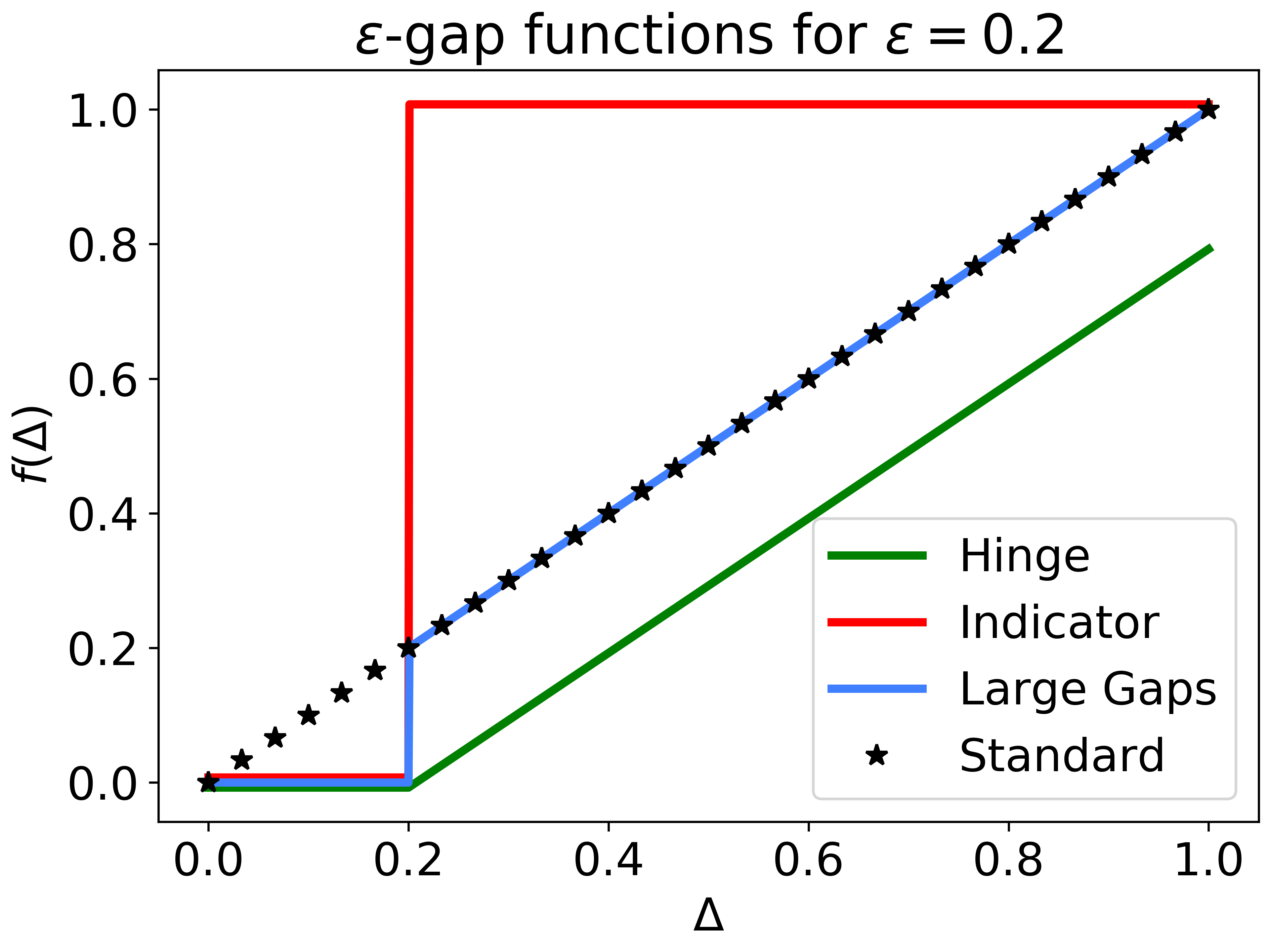
Figure 1: Illustration of different $\epsilon$-gap functions, in comparison to the standard regret $f(\Delta)=\Delta$.

Most MAB algorithms aim to maximize the expected cumulative reward of the agent. Alternatively, algorithms minimize their expected cumulative regret $R(T)=\mathbb{E}\left[\sum_{t=1}^{T}\Delta_{t}\right]$. However, and as previously discussed, this sometimes leads to undesired results. Notably, to identify an optimal arm, algorithms must sufficiently explore all suboptimal arms, which is sometimes infeasible. Nonetheless, existing lower bounds for regret-minimizing algorithms show that any reasonable algorithm cannot avoid such exploration (Lai and Robbins, 1985). To overcome this issue, we suggest minimizing a weaker notion of regret that ignores small gaps. This will allow finding a near-optimal arm much faster. We formally define this criterion as follows:

Definition 1.

For any $\epsilon\in\left[0,1\right]$, a function $f:\left[0,1\right]\rightarrow\mathbb{R}_{+}$ is called an $\epsilon$-gap function if $f(\Delta)=0$ for all $\Delta\in\left[0,\epsilon\right]$ and $f(\Delta)>0$ for all $\Delta>\epsilon$. The lenient regret w.r.t. an $\epsilon$-gap function $f$ is defined as $R_{f}(T)=\mathbb{E}\left[\sum_{t=1}^{T}f\left(\Delta_{t}\right)\right]$.

While it is natural to require of $f$ to increase with $\Delta$, this assumption is not required for the rest of the paper. Moreover, assuming that $f(\Delta)>0$ for all $\Delta>\epsilon$ is only required for the lower bound; for the upper bound, it can be replaced by $f(\Delta)\geq 0$ when $\Delta>\epsilon$. There are three notable examples for $\epsilon$-gap functions (see also Figure 1 for graphical illustration). First, the most natural choice for an $\epsilon$-gap function is the hinge loss $f(\Delta)=\max\left\{\Delta-\epsilon,0\right\}$, which ignores small gaps and increases linearly for larger gaps. Second, we are sometimes interested in maximizing the number of steps where $\epsilon$-optimal arms are played. In this case, we can choose $f(\Delta)=\mathds{1}\left\{\Delta>\epsilon\right\}$. This can be seen as the natural adaptation of $\epsilon$-best-arm identification into a regret criterion. Importantly, notice that this criterion only penalizes sampling of arms with gaps larger than $\epsilon$. This comes with a stark contrast to best-arm identification, where all samples are penalized, whether they are of $\epsilon$-optimal arms or not. Finally, we can choose $f(\Delta)=\Delta\cdot\mathds{1}\left\{\Delta>\epsilon\right\}$. Importantly, when all gaps are larger than $\epsilon$, then this function leads to the standard regret. Thus, all results for $\epsilon$-gap functions also hold for the standard regret when $\Delta_{a}>\epsilon$ for all suboptimal arms.

There are two ways for relating the lenient regret to the standard regret. First, notice that the standard regret can be represented through the $0$-gap function $f(\Delta)=\Delta$. Alternatively, the standard regret can be related to lenient regret w.r.t. the indicator gap-function:

Claim 1.

Let $R(T)=\mathbb{E}\left[\sum_{t=1}^{T}\Delta_{t}\right]$ be the standard regret and define $f_{\epsilon}(\Delta)=\mathds{1}\left\{\Delta>\epsilon\right\}$. Then,

$$R(T)=\int_{\epsilon=0}^{1}R_{f_{\epsilon}}(T)d\epsilon\enspace.$$

The proof is in Section E.1. Specifically, it implies that the standard regret aims to minimize the average lenient regret over different leniency levels. In contrast, our approach allows choosing which leniency level to minimize according to the specific application. By doing so, the designer can adjust the algorithm to its needs, instead of using an algorithm that minimizes the average performance.

3 Lower Bounds

In this section, we prove a problem-dependent lower bound for the lenient regret. Notably, when working with $\epsilon$-gap functions with $\epsilon>0$, we prove that the lower bound behaves inherently different than the case of $\epsilon=0$. Namely, for some problems, the lower bound is sub-logarithmic, in contrast to the $\Omega(\ln T)$ bound for the standard regret.

To prove the lower bound, we require some additional notations. Denote by $\mathcal{D}$, a set of distributions over $\left[0,1\right]$ such that $\nu_{a}\in\mathcal{D}$ for all $a\in\left[K\right]$. A bandit strategy is called consistent over $\mathcal{D}$ w.r.t. an $\epsilon$-gap function $f$ if for any bandit problem with arm distributions in $\mathcal{D}$ and for any $0<\alpha\leq 1$, it holds that $R_{f}(T)=o\left(T^{\alpha}\right)$. Finally, we use $\mathcal{K}_{\mathrm{inf}}$, as was defined in (Burnetas and Katehakis, 1996; Garivier et al., 2019):

$$\mathcal{K}_{\mathrm{inf}}(\nu,x,\mathcal{D})=\inf\left\{\mathrm{KL}(\nu,\nu^{\prime}):\nu^{\prime}\in\mathcal{D},\mathbb{E}\left[\nu^{\prime}\right]>x\right\}\enspace,$$

and by convention, the infimum over an empty set equals $\infty$. We now state the lower bound:

Theorem 1.

For any consistent bandit strategy w.r.t. an $\epsilon$-gap function $f$, for all arms $k\in\left[K\right]$ such that $\Delta_{k}>\epsilon$, it holds that

$$\liminf_{T\to\infty}\frac{\mathbb{E}\left[N_{k}(T+1)\right]}{\ln T}\geq\frac{1}{\mathcal{K}_{\mathrm{inf}}(\nu_{k},\mu^{*}+\epsilon,\mathcal{D})}\enspace.$$ (1)

Specifically, the lenient regret w.r.t. $f$ is lower bounded by

$$\liminf_{T\to\infty}\frac{R_{f}(T)}{\ln T}\geq\sum_{a:\Delta_{a}>\epsilon}\frac{f(\Delta_{a})}{\mathcal{K}_{\mathrm{inf}}(\nu_{a},\mu^{*}+\epsilon,\mathcal{D})}\enspace.$$ (2)

The proof uses the techniques of (Garivier et al., 2019) and can be found in Appendix B. Specifically, choosing $\epsilon=0$ leads to the bound for the standard regret (Burnetas and Katehakis, 1996). As anticipated, both the lenient regret and the number of samples from arms with large gaps decrease as $\epsilon$ increases. This justifies our intuition that removing the penalty from $\epsilon$-optimal arms enables algorithms to reduce the exploration of arms with $\Delta_{a}>\epsilon$.

The fact that the bounds decrease with $\epsilon$ leads to another interesting conclusion – any algorithm that matches the lower bound for some $\epsilon$ is not consistent for any $\epsilon^{\prime}<\epsilon$, since it breaks the lower bound for $\epsilon^{\prime}$. This specifically holds for the standard regret and implies that there is no ‘free lunch’ – achieving the optimal lenient regret for some $\epsilon>0$ leads to non-logarithmic standard regret.

Surprisingly, the lower bound is sub-logarithmic when $\mu^{*}>1-\epsilon$. To see this, notice that in this case, there is no distribution $\nu\in\mathcal{D}$ such that $\mathbb{E}\left[\nu\right]>\mu^{*}+\epsilon$, and thus $\mathcal{K}_{\mathrm{inf}}(\nu_{a},\mu^{*}+\epsilon,\mathcal{D})=\infty$. Intuitively, if the rewards are bounded in $[0,1]$ and some arm has a mean $\mu_{a}>1-\epsilon$, playing it can never incur regret. Identifying that such an arm exists is relatively easy, which leads to low lenient regret. Indeed, we will later present an algorithm that achieves constant regret in this regime.

Finally, and as with most algorithms, we will focus on the set of all problems with rewards bounded in $[0,1]$. In this case, the denominator in Equation 2 is bounded by $\mathcal{K}_{\mathrm{inf}}(\nu_{a},\mu^{*}+\epsilon,\mathcal{D})\geq d(\mu_{a},\mu^{*}+\epsilon)$ (e.g., by applying Lemma 1 of (Garivier et al., 2019)), and equality holds when the arms are Bernoulli-distributed. Since our results should also hold for Bernoulli arms, our upper bound will similarly depend on $d(\mu_{a},\mu^{*}+\epsilon)$.

4 Thompson Sampling for Lenient Regret

Algorithm 1 $\epsilon$-TS for Bernoulli arms

1:Initialize $N_{a}(1)=0$, $S_{a}(1)=0$ and $\hat{\mu}_{a}(1)=0$ for all $a\in\left[K\right]$ $\triangleright$ Blue: Changes from TS

2:for $t=1,\dots,T$ do

3:     for $a=1\dots,K$ do

4:         if $\hat{\mu}_{a}\left(t\right)>1-\epsilon$ then

5:              $\theta_{a}(t)=\hat{\mu}_{a}\left(t\right)$

6:         else

7:              $\alpha_{a}(t)=\left\lfloor\frac{S_{a}(t)}{{\color[rgb]{0,0,0.95}1-\epsilon}}\right\rfloor+1$

8:              $\beta_{a}(t)=N_{a}(t)+2-\alpha_{a}(t)$

9:              $\theta_{a}(t)={\color[rgb]{0,0,0.95}(1-\epsilon)}Y$ for $Y\sim\mathrm{Beta}(\alpha_{a}(t),\beta_{a}(t))$

10:         end if

11:     end for

12:     Play $a_{t}\in\arg\max_{a}\theta_{a}(t)$ (break ties randomly) and observe the reward $X_{t}$

13:     Update $N_{a_{t}}(t+1)=N_{a_{t}}(t)+1$, $\;S_{a_{t}}(t+1)=S_{a_{t}}(t)+X_{t}$ and $\hat{\mu}_{a_{t}}\left(t+1\right)=\frac{S_{a_{t}}(t+1)}{N_{a_{t}}(t+1)}$

14:     For all $a\neq a_{t}$, set $N_{a}(t+1)=N_{a}(t)$, $\;S_{a}(t)=S_{a}(t)$ and $\hat{\mu}_{a}\left(t+1\right)=\hat{\mu}_{a}\left(t\right)$

15:end for

In this section, we present a modified TS algorithm that can be applied with $\epsilon$-gap functions. W.l.o.g., we assume that the rewards are Bernoulli-distributed, i.e., $X_{t}\in\left\{0,1\right\}$; otherwise, the rewards can be randomly rounded (see Agrawal and Goyal (2012) for further details). To derive the algorithm, observe that the lower bound of 1 approaches zero as the optimal arm becomes closer to $1-\epsilon$. Specifically, the lower bound behaves similarly to the regret of the vanilla TS with rewards scaled to $[0,1-\epsilon]$. On the other hand, if the optimal arm is above $1-\epsilon$, we would like to give it a higher priority, so the regret in this case will be sub-logarithmic. This motivates the following $\epsilon$-TS algorithm, presented in Algorithm 1: denote by $\theta_{a}(t)$, the sample from the posterior of arm $a$ at round $t$, and recall that TS algorithm choose arms by $a_{t}\in\arg\max_{a}\theta_{a}(t)$. For any arm with $\hat{\mu}_{a}(t)\leq 1-\epsilon$, we fix its posterior to be a scaled Beta distribution, such that the range of the posterior is $\left[0,1-\epsilon\right]$, but its mean (approximately) remains $\hat{\mu}_{a}(t)$ (lines 7-9). If $\hat{\mu}_{a}(t)>1-\epsilon$, we set the posterior to $\theta_{a}(t)=\hat{\mu}_{a}(t)>1-\epsilon$ (line 5), which gives this arm a higher priority than any arm with $\hat{\mu}_{a}(t)\leq 1-\epsilon$. Notice that $\epsilon$-TS does not depend on the specific $\epsilon$-gap function. Intuitively, this is since it suffices to match the number of suboptimal plays in Equation 1, that only depends on $\epsilon$. The algorithm enjoys the following asymptotic lenient regret:

Theorem 2.

Let $f$ be an $\epsilon$-gap function. Then, the lenient regret of $\epsilon$-TS w.r.t. $f$ is

$$\limsup_{T\to\infty}\frac{R_{f}(T)}{\ln T} \leq\sum_{a:\Delta_{a}>\epsilon}\frac{f(\Delta_{a})}{d\left(\frac{\mu_{a}}{1-\epsilon},\frac{\mu^{*}}{1-\epsilon}\right)}\leq 4(1-\epsilon)\sum_{a:\Delta_{a}>\epsilon}\frac{f(\Delta_{a})}{d(\mu_{a},\mu^{*}+\epsilon)}\enspace.$$ (3)

Moreover, if $\mu^{*}>1-\epsilon$, then $R_{f}(T)=\mathcal{O}(1)$.

The proof can be found in the following section. In our context, the $\mathcal{O}$ notation hides constants that depend on the mean of the arms and $\epsilon$. Notice that 2 matches the lower bound of 1 for the set of all bounded distributions (and specifically for Bernoulli arms), up to an absolute constant. Notably, when $\mu^{*}>1-\epsilon$, we prove that the regret is constant, and not only sub-logarithmic, as the lower bound suggests. Specifically in this regime, an algorithm can achieve constant lenient regret by identifying an arm with a mean greater than $1-\epsilon$ and exploiting it. However, the algorithm does not know whether such an arm exists, and if there is no such arm, a best arm-identification scheme will perform poorly. Our algorithm naturally identifies such arms when they exist, while maintaining good lenient regret otherwise. Similarly, algorithms such as of Bubeck et al. (2013) cannot be applied to achieve constant regret, since they require knowing the value of the optimal arm, which is even a stronger requirement than knowing that $\mu^{*}>1-\epsilon$.

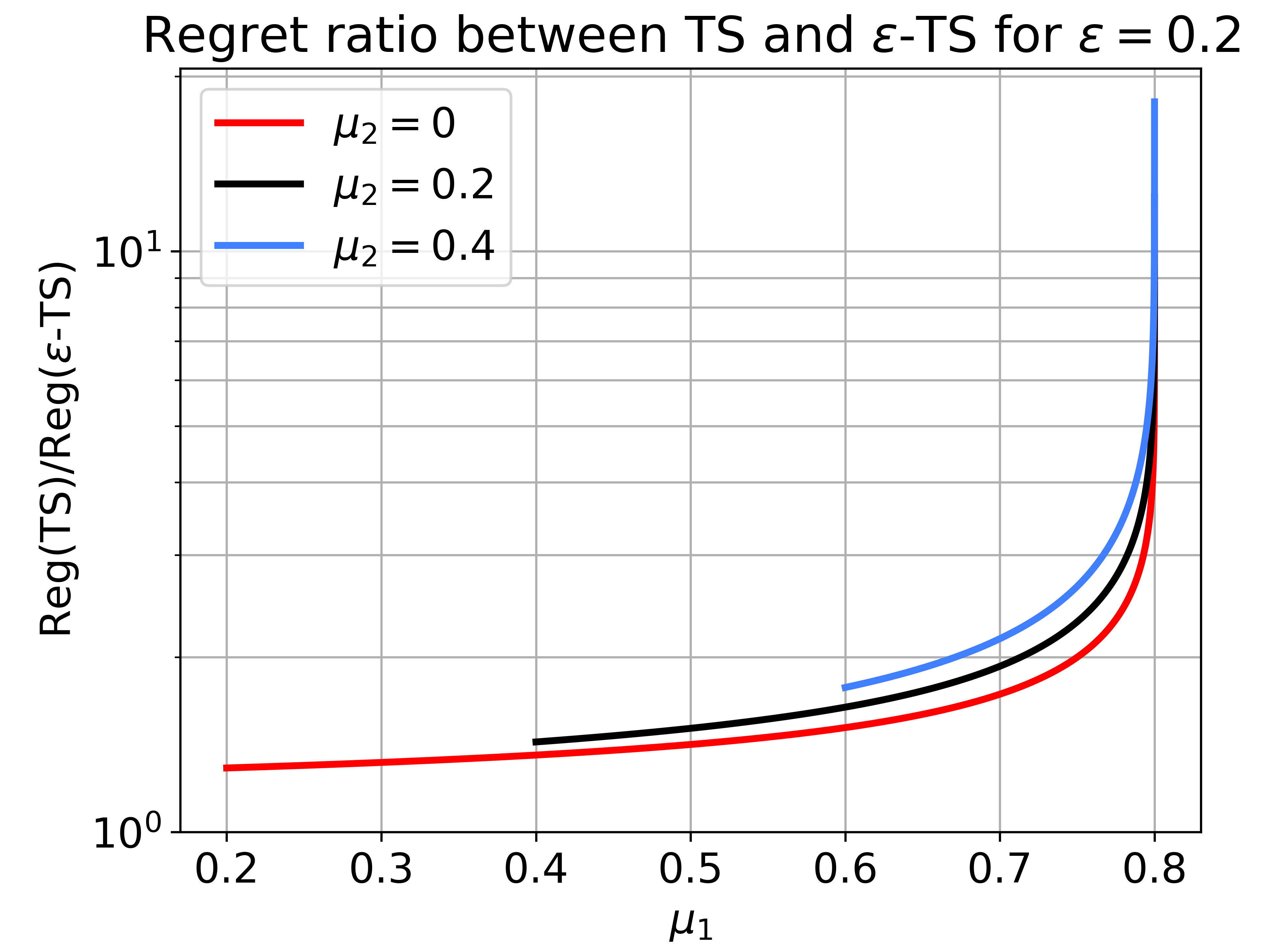
Figure 2: Ratio between the asymptotic lenient regret bounds of TS and $\epsilon$-TS for two-armed problems with $\epsilon=0.2$, as a function of the optimal arm $\mu_{1}$.

Comparison to MAB algorithms: Asymptotically optimal MAB algorithms sample suboptimal arms according to the lower bound, i.e., for any suboptimal arm $a$, $\limsup_{T\to\infty}\frac{N_{a}(T)}{\ln T}\leq\frac{1}{d\left(\mu_{a},\mu^{*}\right)}$. This, in turn, leads to a lenient regret bound of

$$\limsup_{T\to\infty}\frac{R_{f}(T)}{\ln T} \leq\sum_{a:\Delta_{a}>\epsilon}\frac{f(\Delta_{a})}{d\left(\mu_{a},\mu^{*}\right)}$$ (4)

that holds for both the vanilla TS (Kaufmann et al., 2012) and KL-UCB (Garivier and Cappé, 2011). First notice that the bound of Equation 3, that depends on $d\left(\frac{\mu_{a}}{1-\epsilon},\frac{\mu^{*}}{1-\epsilon}\right)$, strictly improves the bounds for the standard algorithms (see Appendix E.4 for further details). Moreover, $\epsilon$-TS achieves constant regret when $\mu^{*}>1-\epsilon$, and its regret quickly diminishes when approaching this regime. This comes in contrast to standard MAB algorithms, that achieve logarithmic regret in these regimes. To illustrate the improvement of $\epsilon$-TS, in comparison to standard algorithms, we present the ratio between the asymptotic bounds of Equations (4) and (3) in Figure 2.

Before presenting the proof, we return to the $\epsilon$-gap function $f(\Delta)=\Delta\cdot\mathds{1}\left\{\Delta>\epsilon\right\}$. Recall that this function leads to the standard regret when all gaps are larger than $\epsilon$. Thus, our algorithm can be applied in this case to greatly improve the performance (from the bound of Equation 4 to the bound of Equation 3), even in terms of the standard regret.

4.1 Regret Analysis

In this section, we prove the regret bound of 2. For the analysis, we assume w.l.o.g. that the arms are sorted in a decreasing order and all suboptimal arms have gaps $\Delta_{a}>\epsilon$, i.e. $\mu^{*}=\mu_{1}\geq\mu_{1}-\epsilon>\mu_{2}\geq\dots\geq\mu_{K}$. If there are additional arms with gaps $\Delta_{a}\leq\epsilon$, playing them will cause no regret and the overall lenient regret will only decrease (see Section D.1 or Appendix A in (Agrawal and Goyal, 2012) for further details). We also assume that $\epsilon<1$, as otherwise $f(\Delta_{a})=0$ for all $a\in\left[K\right]$. Under these assumptions, we now state a more detailed bound for the lenient regret, that also includes a finite-time behavior:

Theorem 3.

Let $f$ be an $\epsilon$-gap function. If $\mu_{1}>1-\epsilon$, there exists some constants $b=b(\mu_{1},\mu_{2},\epsilon)\in\left(0,1\right)$, $C_{b}=C_{b}(\mu_{1},\mu_{2},\epsilon)$ and $L_{1}=L_{1}(\mu_{1},\epsilon,b)$ such that

$$R_{f}(T) \leq\sum_{a=2}^{K}\frac{f(\Delta_{a})}{d(1-\epsilon,\mu_{a})}+\max_{a}f(\Delta_{a})\left(C_{b}+L_{1}+\frac{\pi^{2}/6}{d(1-\epsilon,\mu_{1})}\right)=\mathcal{O}(1)\enspace.$$ (5)

If $\mu_{1}\leq 1-\epsilon$, then for any $c>0$, there exist additional constants $L_{2}=L_{2}(b,\epsilon)$ and $x_{a,c}=x_{a,c}(\mu_{1},\mu_{a},\epsilon)$ such that for $\eta(t)=\max\left\{\mu_{1}-\epsilon,\mu_{1}-2\sqrt{\frac{6\ln t}{t^{b}}}\right\}$,

$$R_{f}(T) \!\leq\sum_{a=2}^{K}f(\Delta_{a})\left((1+c)^{2}\max_{t\in\left[T\right]}\left\{\frac{\ln t}{d\left(\frac{\mu_{a}}{1-\epsilon},\frac{\eta(t)}{1-\epsilon}\right)}\right\}+2+\frac{1}{c}+\frac{1}{d(x_{a,c},\mu_{a})}\right)+\max_{a}f(\Delta_{a})\left(C_{b}+L_{2}+6\right).$$ (6)

Proof.

We decompose the regret similarly to (Kaufmann et al., 2012) and show that with high probability, the optimal arm is sampled polynomially, i.e., $N_{1}(t)=\Omega(t^{b})$ for some $b\in\left(0,1\right)$. Formally, let $\eta(t)$ be some function such that $\mu_{1}-\epsilon\leq\eta(t)<\mu_{1}$ for all $t\in\left[T\right]$, and for brevity, let $f_{\max}=\max_{a}f(\Delta_{a})$. Also, recall that the lenient regret is defined as $R_{f}(T)=\mathbb{E}\left[\sum_{t=1}^{T}f\left(\Delta_{t}\right)\right]$. Then, the lenient regret can be decomposed to

$$R_{f}( T)=\sum_{t=1}^{T}\mathbb{E}\left[f(\Delta_{t})\mathds{1}\left\{\theta_{1}(t)>\eta(t)\right\}\right]+\sum_{t=1}^{T}\mathbb{E}\left[f(\Delta_{t})\mathds{1}\left\{\theta_{1}(t)\leq\eta(t)\right\}\right]$$

$$\leq\sum_{t=1}^{T}\mathbb{E}\left[f(\Delta_{t})\mathds{1}\left\{\theta_{1}(t)>\eta(t)\right\}\right]+f_{\max}\sum_{t=1}^{T}\mathbb{E}\left[\mathds{1}\left\{\theta_{1}(t)\leq\eta(t)\right\}\right]$$

$$=\sum_{t=1}^{T}\sum_{a=2}^{K}f(\Delta_{a})\mathbb{E}\left[\mathds{1}\left\{a_{t}=a,\theta_{1}(t)>\eta(t)\right\}\right]+f_{\max}\sum_{t=1}^{T}\mathbb{E}\left[\mathds{1}\left\{\theta_{1}(t)\leq\eta(t)\right\}\right]\enspace.$$

Replacing the expectations of indicators with probabilities and dividing the second term to the case where $a_{1}$ was sufficiently and insufficiently sampled, we get

$$R_{f}( T)\leq\sum_{a=2}^{K}f(\Delta_{a})\underbrace{\sum_{t=1}^{T}\Pr\left\{a_{t}=a,\theta_{1}(t)>\eta(t)\right\}}_{(A)}+f_{\max}\underbrace{\sum_{t=1}^{T}\Pr\left\{\theta_{1}(t)\leq\eta(t),N_{1}(t)>(t-1)^{b}\right\}}_{(B)}$$

$$\qquad+f_{\max}\underbrace{\sum_{t=1}^{T}\Pr\left\{N_{1}(t)\leq(t-1)^{b}\right\}}_{(C)}\enspace.$$ (7)

The first part of the proof consists of bounding term $(C)$, i.e., showing that the optimal arm is sampled polynomially with high probability. We do so in the following proposition:

Proposition 2.

There exist constants $b=b(\mu_{1},\mu_{2},\epsilon)\in(0,1)$ and $C_{b}=C_{b}(\mu_{1},\mu_{2},\epsilon)<\infty$ such that

$$\sum_{t=1}^{T}\Pr\left\{N_{1}(t)\leq(t-1)^{b}\right\}\leq C_{b}\enspace.$$

The proof follows the lines of Proposition 1 in (Kaufmann et al., 2012) and can be found in Appendix C. To bound $(A)$ and $(B)$, we divide the analysis into two cases: $\mu_{1}>1-\epsilon$ and $\mu_{1}\leq 1-\epsilon$.

First case:

$\mu_{1}>1-\epsilon$.

In this case, we fix $\eta(t)=1-\epsilon$. For $(A)$, observe that if $a_{t}=a$ and $\theta_{1}(t)>1-\epsilon$, then $\theta_{a}(t)>1-\epsilon$, which also implies that $\hat{\mu}_{a}\left(t\right)>1-\epsilon$ (to see this, notice that if $\hat{\mu}_{a}\left(t\right)\leq 1-\epsilon$, then $\theta_{a}(t)=(1-\epsilon)Y\leq 1-\epsilon$). However, since $\Delta_{a}>\epsilon$ for all $a\neq 1$, all suboptimal arms have means $\mu_{a}<1-\epsilon$. Thus, when $N_{a}(t)$ becomes large, the probabilities in $(A)$ quickly diminish and this term can be bounded by constant. Formally, we write

$$\sum_{t=1}^{T}\Pr\left\{a_{t}=a,\theta_{1}(t)>1-\epsilon\right\} \leq\sum_{t=1}^{T}\Pr\left\{a_{t}=a,\theta_{a}(t)>1-\epsilon\right\}=\sum_{t=1}^{T}\Pr\left\{a_{t}=a,\hat{\mu}_{a}\left(t\right)>1-\epsilon\right\},$$

and bound this term using the following lemma (see Section D.2 for the proof):

Lemma 3.

For any arm $a\in\left[K\right]$, if $x>\mu_{a}$, then

$$\sum_{t=1}^{T}\Pr\left\{a_{t}=a,\hat{\mu}_{a}\left(t\right)>x\right\}\leq\frac{1}{d(x,\mu_{a})}\enspace.$$

Similarly, in $(B)$, $\theta_{1}(t)\leq 1-\epsilon$ implies that $\hat{\mu}_{1}\left(t\right)\leq 1-\epsilon$, and since $N_{1}(t)$ is large, this event has a low probability. We formalize this intuition in 4, whose proof can be found in Section D.3.

Lemma 4.

Assume that $\mu_{1}>1-\epsilon$, and for any $b\in\left(0,1\right)$, let $L_{1}(\mu_{1},\epsilon,b)$ such that for all $t\geq L_{1}(\mu_{1},\epsilon,b)$, it holds that $(t-1)^{b}\geq\frac{2\ln t}{d(1-\epsilon,\mu_{1})}+1$. Then,

$$\sum_{t=1}^{T}\Pr\left\{\theta_{1}(t)\leq 1-\epsilon,N_{1}(t)>(t-1)^{b}\right\}\leq L_{1}(\mu_{1},\epsilon,b)+\frac{\pi^{2}/6}{d(1-\epsilon,\mu_{1})}\enspace.$$

Substituting both lemmas and 2 into Equation 7 leads to Equation 5.

Second case:

$\mu_{1}\leq 1-\epsilon$.

For this case, we fix $\eta(t)=\max\left\{\mu_{1}-\epsilon,\mu_{1}-2\sqrt{\frac{6\ln t}{(t-1)^{b}}}\right\}$. To bound $(A)$, we adapt the analysis of (Agrawal and Goyal, 2013a) and decompose this term into two parts: (i) the event where the empirical mean $\hat{\mu}_{a}\left(t\right)$ is far above $\mu_{a}$, and (ii) the event where $\hat{\mu}_{a}\left(t\right)$ is close to $\mu_{a}$ and $\theta_{a}(t)$ is above $\eta(t)$. Doing so leads to 5, whose proof is in Section D.4:

Lemma 5.

Assume that $\mu_{1}\leq 1-\epsilon$ and $\eta(t)\in[\mu_{1}-\epsilon,\mu_{1})$ for all $t\in\left[T\right]$. Then, for any $c>0$,

$$\sum_{t=1}^{T}\Pr\left\{a_{t}=a,\theta_{1}(t)>\eta(t)\right\}\leq(1+c)^{2}\max_{t\in\left[T\right]}\left\{\frac{\ln t}{d\left(\frac{\mu_{a}}{1-\epsilon},\frac{\eta(t)}{1-\epsilon}\right)}\right\}+2+\frac{1}{c}+\frac{1}{d(x_{a,c},\mu_{a})}\enspace,$$

where $x_{a,c}\in\left(\mu_{a},\mu_{1}-\epsilon\right)$ is such that $d\left(\frac{x_{a,c}}{1-\epsilon},\frac{\mu_{1}-\epsilon}{1-\epsilon}\right)=\frac{1}{1+c}d\left(\frac{\mu_{a}}{1-\epsilon},\frac{\mu_{1}-\epsilon}{1-\epsilon}\right)$.

For $(B)$, we provide the following lemma (see Section D.5 for the proof):

Lemma 6.

Assume that $\mu_{1}\leq 1-\epsilon$ and let $\eta(t)=\max\left\{\mu_{1}-\epsilon,\mu_{1}-2\sqrt{\frac{6\ln t}{(t-1)^{b}}}\right\}$. Also, let $L_{2}(b,\epsilon)\geq 2$ such that for all $t\geq L_{2}(b,\epsilon)$, it holds that $\eta(t)>\mu_{1}-\epsilon$. Then,

$$\sum_{t=1}^{T}\Pr\left\{\theta_{1}(t)\leq\eta(t),N_{1}(t)>(t-1)^{b}\right\}\leq L_{2}(b,\epsilon)+6$$

Substituting both lemmas and 2 into Equation 7 results with Equation 6 and concludes the proof of Theorem 3. ∎

Proof sketch of 2.

It only remains to prove the asymptotic rate of 2, using the finite-time bound of Theorem 3. To do so, notice that the denominator in Equation 6 asymptotically behaves as $d\left(\frac{\mu_{a}}{1-\epsilon},\frac{\mu_{1}}{1-\epsilon}\right)$, which leads to the first bound of the theorem. On the other hand, the denominator of the second bound depends on $d\left(\mu_{a},\mu_{1}+\epsilon\right)$. We prove that when $\Delta_{a}>\epsilon$, these two quantities are closely related:

Lemma 7.

For any $\epsilon\in\left[0,\frac{1}{2}\right)$, any $p\in[0,1-2\epsilon)$ and any $q\in[p+\epsilon,1-\epsilon)$,

$$d\left(\frac{p}{1-\epsilon},\frac{q}{1-\epsilon}\right)\geq\frac{1}{4(1-\epsilon)}d(p,q+\epsilon)\enspace.$$

The proof of this lemma can be found in Section E.2. This immediately leads to the desired asymptotic rate, but for completeness, we provide the full proof of the theorem in Section D.6. ∎

5 Experiments

In this section, we present an empirical evaluation of $\epsilon$-TS. Specifically, we compare $\epsilon$-TS to the vanilla TS on two different gap functions: $f(\Delta)=\Delta$, which leads to the standard regret, and the hinge function $f(\Delta)=\max\left\{\Delta-\epsilon,0\right\}$. All evaluations were performed for $\epsilon=0.2$ over $50,000$ different seeds and are depicted in Figure 3. We also refer the readers to Appendix F, where additional statistics of the simulations are presented, alongside additional tests that were omitted due to space limits. We tested 4 different scenarios – when the optimal arm is smaller or larger than $1-\epsilon$ (left and right columns, respectively), and when the minimal gap is larger or smaller than $\epsilon$ (top and bottom rows, respectively). Importantly, when the minimal gap is larger than $\epsilon$, the standard regret can be written using the $\epsilon$-gap function $f(\Delta)=\Delta\cdot\mathds{1}\left\{\Delta>\epsilon\right\}$. Indeed, one can observe that when $\Delta_{a}>\epsilon$ for all suboptimal arms, $\epsilon$-TS greatly improves the performance, in comparison to the vanilla TS. Similarly, when $\mu^{*}>1-\epsilon$, the lenient regret of $\epsilon$-TS converges to a constant, as can be expected from 2. On the other hand, the lenient regret of the vanilla TS continues to increase.

Next, we move to simulations where the suboptimality gap is smaller than $\epsilon$. In such cases, the standard regret cannot be represented as an $\epsilon$-gap function, and $\epsilon$-TS is expected to perform worse on this criterion than the vanilla TS. Quite surprisingly, when $\mu^{*}=0.5$, $\epsilon$-TS still surpasses the vanilla TS. In Appendix F, we show that TS beats $\epsilon$-TS only after $20,000$ steps. On the other hand, when $\mu^{*}=0.9$, the standard regret of $\epsilon$-TS increases linearly. This is since with finite probability, the algorithm identifies that $\mu_{2}=0.85>1-\epsilon$ at a point where the empirical mean of the optimal arm is smaller than $1-\epsilon$. Then, the algorithm only exploits $a=2$ and will never identify that $a=1$ is the optimal arm. Nonetheless, we emphasize that $\epsilon$-TS still outperforms the vanilla TS in terms of the lenient regret, as can be observed for the hinge-function.

To conclude this section, the simulations clearly demonstrate the tradeoff when optimizing the lenient regret: when near-optimal solutions are adequate, then the performance can be greatly improved. On the other hand, in some cases, it leads to major degradation in the standard regret.

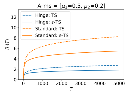
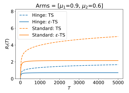
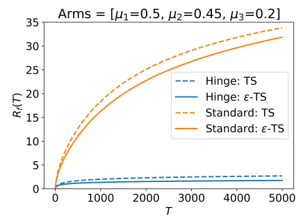
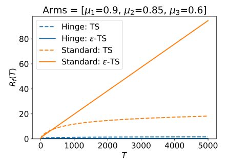
Figure 3: Evaluation of $\epsilon$-TS and vanilla TS with $\epsilon=0.2$ and Bernoulli rewards. ‘Hinge’ is the $\epsilon$-gap function $f(\Delta)=\max\left\{\Delta-\epsilon,0\right\}$ and ‘Standard’ is the $0$-gap function $f(\Delta)=\Delta$, which leads to the standard regret. Top row – the minimal gap is $\Delta_{2}=0.3>\epsilon$; therefore, $\epsilon$-TS enjoys performance guarantees also for the standard regret. Bottom row – the minimal gap is $\Delta_{2}=0.05<\epsilon$; thus, the standard regret $f(\Delta)=\Delta$ is not an $\epsilon$-gap function, and $\epsilon$-TS has no guarantees for this case.

6 Summary and Future Work

In this work, we introduced the notion of lenient regret w.r.t. $\epsilon$-gap functions. We proved a lower bound for this setting and presented the $\epsilon$-TS algorithm, whose performance matches the lower bound, up to a constant factor. Specifically, we showed that the $\epsilon$-TS greatly improves the performance when a lower bound on the gaps is known. Finally, we performed an empirical evaluation that demonstrates the advantage of our new algorithm when optimizing the lenient regret.

We believe that our work opens up many interesting directions. First, while we suggest a TS algorithm for our settings, it is interesting to devise its UCB counterpart. Moreover, there are alternative ways to define $\epsilon$-gap functions that should be explored, e.g., functions that do not penalize arms with mean larger than $\mu^{*}\cdot(1-\epsilon)$ (multiplicative leniency). This can also be done by borrowing other approximation concepts from best arm identification. For example, not penalizing arms that exceed some threshold (as in good arm identification Kano et al. (2019)), or not penalizing the choice of any one of the top $m$ of the arms (Chaudhuri and Kalyanakrishnan, 2017).

We also believe that the concept of lenient regret criteria can be extended to many different settings. It is especially relevant when problems are large, e.g., in combinatorial problems (Chen et al., 2016a), and can also be extended to reinforcement learning (Sutton and Barto, 2018). Notably, and as previously stated, there is some similarity between the $\epsilon$-gap function $f(\Delta)=\mathds{1}\left\{\Delta>\epsilon\right\}$ and the sample-complexity criterion in RL (Kakade et al., 2003), and our analysis might allow proving new results for this criterion.

Finally, we explored the notion of lenient regret for stochastic MABs. Another possible direction is adapting the lenient regret to adversarial MABs, and potentially for online learning. In these settings, the convergence rates are typically $\mathcal{O}(\sqrt{T})$, and working with weaker notions of regret might lead to logarithmic convergence rates.

Appendix A Useful Results for the Analysis

Beta and Binomial distributions:

• Beta distribution: For any $\alpha,\beta>0$, we say that $X\sim\mathrm{Beta}(\alpha,\beta)$, if for any $x\in\left[0,1\right]$, its pdf is

  $$f_{X}(x)=f^{\mathrm{Beta}}_{\alpha,\beta}(x)=\frac{1}{B(\alpha,\beta)}x^{\alpha-1}(1-x)^{\beta-1}\enspace,$$

  where $B(\alpha,\beta)$ is the Beta function.

• Binomial distribution: If $n$ is a positive integer and $p\in\left[0,1\right]$, we say that $X\sim Bin(n,p)$, if for any $k\in\left[0,\dots,n\right]$, its pdf is

  $$f_{X}(k)=f^{B}_{n,p}(k)=\binom{n}{k}p^{k}(1-p)^{n-k}\enspace.$$

The cdf of both distributions is related through the ‘Beta-Binomial trick’ [Agrawal and Goyal, 2012]:

Fact 1.

If $\alpha,\beta$ are positive integers and $x\in\left[0,1\right]$, then

$$F^{\mathrm{Beta}}_{\alpha,\beta}(x)=1-F^{B}_{\alpha+\beta-1,x}(\alpha-1)\enspace.$$

Useful concentration bounds:

we now present two useful concentration bounds that will be used throughout the paper.

Fact 2 (Hoeffding’s Inequality).

Let $X_{1},\dots,X_{n}\in\left[0,1\right]$ be independent random variables with common expectation $\mu$ and let $t\geq 0$. Then,

$$\Pr\left\{\frac{1}{n}\sum_{i=1}^{n}X_{i}\geq\mu+t\right\}\leq e^{-2nt^{2}}$$

$$\Pr\left\{\frac{1}{n}\sum_{i=1}^{n}X_{i}\leq\mu-t\right\}\leq e^{-2nt^{2}}$$

Fact 3 (Chernoff-Hoeffding Bound).

Let $X_{1},\dots,X_{n}\in\left\{0,1\right\}$ be independent Bernoulli random variables with common expectation $\mu$ and let $t\geq 0$. Then,

$$\Pr\left\{\frac{1}{n}\sum_{i=1}^{n}X_{i}\geq\mu+t\right\}\leq e^{-n\cdot d(\mu+t,\mu)}$$

$$\Pr\left\{\frac{1}{n}\sum_{i=1}^{n}X_{i}\leq\mu-t\right\}\leq e^{-n\cdot d(\mu-t,\mu)}$$

Appendix B Proof of Theorem 1

In this appendix, we prove the lower bound of Section 3. The proof adapts the techniques of [Garivier et al., 2019] and require a fundamental result in their paper: for any fixed bandit strategy, any sets of arm distributions ${\underline{\nu}},{\underline{\nu}}^{\prime}$ and any $k\in\left[K\right]$ and any $T>0$, it holds that

$$\sum_{a=1}^{K}\mathbb{E}_{\underline{\nu}}\left[N_{a}(T+1)\right]\mathrm{KL}(\nu_{a},\nu_{a}^{\prime})\geq d\left(\frac{\mathbb{E}_{\underline{\nu}}\left[N_{k}(T+1)\right]}{T},\frac{\mathbb{E}_{{\underline{\nu}}^{\prime}}\left[N_{k}(T+1)\right]}{T}\right)$$ (8)

The inequality is a direct result of Equation (6) in [Garivier et al., 2019] with $Z=N_{k}(T+1)/T$.

See 1

Proof.

We start by proving Equation 1. To do so, we follow the proof of Theorem 1 of [Garivier et al., 2019]. Denote the arm distribution by ${\underline{\nu}}$ and for clarity, denote the lenient regret under arm distribution ${\underline{\nu}}$ by $R_{f,{\underline{\nu}}}(T)$. Also, let $k$ be some suboptimal arm with $\Delta_{k}>\epsilon$ and let ${\underline{\nu}}^{\prime}$ be a bandit problem such that $\nu_{a}^{\prime}=\nu_{a}$ for all $a\neq k$ and $\nu_{k}^{\prime}\in\mathcal{D}$ is some distribution with $\mathbb{E}\left[\nu_{k}^{\prime}\right]>\mu^{*}+\epsilon$. If such distribution does not exist, then $\mathcal{K}_{\mathrm{inf}}(\nu,\mu^{*}+\epsilon,\mathcal{D})=\infty$ and the lower bound trivially holds. Next, by applying Equation 8 and noting that for all $a\neq k$, $\mathrm{KL}(\nu_{a},\nu_{a}^{\prime})=0$, we get

$$\mathbb{E}_{\underline{\nu}}\left[N_{k}(T+1)\right]\mathrm{KL}(\nu_{k},\nu_{k}^{\prime})\geq d\left(\frac{\mathbb{E}_{\underline{\nu}}\left[N_{k}(T+1)\right]}{T},\frac{\mathbb{E}_{{\underline{\nu}}^{\prime}}\left[N_{k}(T+1)\right]}{T}\right)$$

Next, see that the for all $p,q\in\left[0,1\right]$,

$$d(p,q) =p\ln\frac{p}{q}+(1-p)\ln\frac{1-p}{1-q}$$

$$=(1-p)\ln\frac{1}{1-q}+\underbrace{p\ln p+(1-p)\ln(1-p)}_{\geq-\ln 2}+\underbrace{p\ln\frac{1}{q}}_{\geq 0}$$

$$\geq(1-p)\ln\frac{1}{1-q}-\ln 2$$

and combining both inequalities yields

$$\mathbb{E}_{\underline{\nu}}\left[N_{k}(T+1)\right]\mathrm{KL}(\nu_{k},\nu_{k}^{\prime})\geq\left(1-\frac{\mathbb{E}_{\underline{\nu}}\left[N_{k}(T+1)\right]}{T}\right)\ln\frac{T}{T-\mathbb{E}_{{\underline{\nu}}^{\prime}}\left[N_{k}(T+1)\right]}-\ln 2\enspace.$$ (9)

To further bound this term, notice that the lenient regret for bandit problem ${\underline{\nu}}^{\prime}$ can be written as $R_{f,{\underline{\nu}}^{\prime}}(T)=\sum_{a=1}^{K}f\left(\Delta_{a}^{\prime}\right)\mathbb{E}_{{\underline{\nu}}^{\prime}}\left[N_{a}(T+1)\right]$. By construction, the optimal arm in ${\underline{\nu}}^{\prime}$ is $k$, with gaps $\Delta_{a}^{\prime}=\mathbb{E}\left[\nu_{k}^{\prime}\right]-\mathbb{E}\left[\nu_{a}\right]>\epsilon$ for all $a\neq k$. Since $f$ is an $\epsilon$-gap function, this also implies that $f(\Delta_{a}^{\prime})>0$ for all $a\neq k$ and $f(\Delta_{k}^{\prime})=0$. Finally, as the bandit strategy is consistent, it holds that

$$T-\mathbb{E}_{{\underline{\nu}}^{\prime}}\left[N_{k}(T+1)\right] =\sum_{a\neq k}\mathbb{E}_{{\underline{\nu}}^{\prime}}\left[N_{a}(T+1)\right]$$

$$\leq\frac{1}{\min_{a\neq k}f(\Delta_{a}^{\prime})}\sum_{a\neq k}f(\Delta_{a}^{\prime})\mathbb{E}_{{\underline{\nu}}^{\prime}}\left[N_{a}(T+1)\right]$$

$$=\frac{1}{\min_{a\neq k}f(\Delta_{a}^{\prime})}R_{f,{\underline{\nu}}^{\prime}}(T)$$

$$=o(T^{\alpha})\enspace,$$

for all $0<\alpha\leq 1$. Specifically, for $T$ large enough, $T-\mathbb{E}_{{\underline{\nu}}^{\prime}}\left[N_{k}(T+1)\right]\leq T^{\alpha}$, and thus

$$\liminf_{T\to\infty}\frac{1}{\ln T}\ln\frac{T}{T-\mathbb{E}_{{\underline{\nu}}^{\prime}}\left[N_{k}(T+1)\right]}\geq\frac{1}{\ln T}\ln\frac{T}{T^{\alpha}}=1-\alpha\enspace.$$ (10)

Next, notice that for all arms such that $\Delta_{k}>\epsilon$, we have $f(\Delta_{k})>0$, and thus

$$\mathbb{E}_{\underline{\nu}}\left[N_{k}(T+1)\right]=\frac{1}{f(\Delta_{k})}\left(f(\Delta_{k})\mathbb{E}_{\underline{\nu}}\left[N_{k}(T+1)\right]\right)\leq\frac{1}{f(\Delta_{k})}R_{f,{\underline{\nu}}}(T)=o(T)\enspace,$$

which implies that

$$\liminf_{T\to\infty}\left(1-\frac{\mathbb{E}_{\underline{\nu}}\left[N_{k}(T+1)\right]}{T}\right)=1$$

Substituting this relation and Equation 10 into Equation 9 yields

$$\liminf_{T\to\infty}\frac{\mathbb{E}\left[N_{k}(T+1)\right]}{\ln T}\geq\frac{1}{\mathrm{KL}(\nu_{k},\nu_{k}^{\prime})}\enspace.$$

To conclude the proof of Equation 1, we take the supremum of the r.h.s. over all distributions $\nu_{k}^{\prime}\in\mathcal{D}$ such that $\mathbb{E}\left[\nu_{k}^{\prime}\right]>\mu^{*}+\epsilon$, which leads to $\mathcal{K}_{\mathrm{inf}}(\nu_{k},\mu^{*}+\epsilon,\mathcal{D})>0$ in the r.h.s.. We also remind that if such distribution does not exist, then $\mathcal{K}_{\mathrm{inf}}(\nu_{k},\mu^{*}+\epsilon,\mathcal{D})=\infty$ and the bound trivially holds.

For Equation 2, we write the lenient regret as $R_{f}(T)=\sum_{a=1}^{K}f\left(\Delta_{a}\right)\mathbb{E}\left[N_{a}(T+1)\right]$. Substituting Equation 1 into this relation leads to the desired result. ∎

Appendix C Proof of Proposition 2

In this appendix, we prove 2, including the additional lemmas that we require for the proof: See 2

Proof.

We closely follow the proof of Proposition 1 of [Kaufmann et al., 2012], with many modifications due to the different posterior distribution. Let $t$ be some fixed time index. If the $j^{th}$ play of the optimal arm happened before $t$, we denote its time by $\tau_{j}$. Otherwise we say that $\tau_{j}=t$ and also denote $\tau_{0}=0$. In addition, let $\xi_{j}=(\tau_{j+1}-1)-\tau_{j}$ be the number of time steps between the $j^{th}$ and the $(j+1)^{th}$ play of the optimal arm. In these steps, only suboptimal arms are played, and we have $\sum_{a=2}^{K}N_{a}(t+1)\geq\sum_{j=0}^{N_{1}(t+1)}\xi_{j}$. Using this notation, we can bound the event that $N_{1}(t+1)\leq t^{b}$ by

$$\Pr\left\{N_{1}(t+1)\leq t^{b}\right\} =\Pr\left\{\sum_{a=2}^{K}N_{a}(t+1)>t-t^{b}\right\}\leq\Pr\left\{\exists j\in\left\{0,\dots,\left\lfloor t^{b}\right\rfloor\right\}:\xi_{j}\geq t^{1-b}-1\right\}$$

$$\leq\sum_{j=0}^{\left\lfloor t^{b}\right\rfloor}\Pr\left\{\xi_{j}\geq t^{1-b}-1\right\}\enspace.$$

Thus, we are interested in bounding the probability of the events $E_{j}=\left\{\xi_{j}\geq t^{1-b}-1\right\}$. Define the interval $\mathcal{I}_{j}=\left\{\tau_{j}+1,\dots,\tau_{j}+\left\lceil t^{1-b}-1\right\rceil\right\}$, and notice that under $E_{j}$, it is included in $\left\{\tau_{j}+1,\dots,\tau_{j+1}-1\right\}$. This also implies that under $E_{j}$, for any $s\in\mathcal{I}_{j}$ we have that $s\leq t$. We further decompose the interval into $K$ smaller intervals, defined as

$$\mathcal{I}_{j,l} =\left\{\tau_{j}+\left\lceil\frac{(l-1)(t^{1-b}-1)}{K}\right\rceil+1,\dots,\tau_{j}+\left\lceil\frac{l(t^{1-b}-1)}{K}\right\rceil\right\}\enspace, l=1\dots,K$$

When $E_{j}$ holds, observe that only suboptimal arms are sampled in these intervals. Therefore, in each them, at least one of the suboptimal arms will be sampled $\frac{\left\lvert\mathcal{I}_{j,l}\right\rvert}{K}$ times. Intuitively, for enough samples, the posterior of this arm will be tightly concentrated around its mean, and this arm will be sampled rarely for the rest of $\mathcal{I}_{j}$. After $K-1$ such intervals, all the suboptimal arms should be highly concentrated around their mean. Then, the probability of not sampling the optimal arm in the last interval should be very low. To formalize this, we employ the notion of saturated and unsaturated arms, similarly to [Kaufmann et al., 2012]:

Definition 2.

Let $t$ be fixed. An arm $a\neq 1$ is called saturated at time $s\leq t$ if $N_{a}(s)\geq\frac{32\ln t}{(\Delta_{a}-\epsilon)^{2}}\triangleq C_{a}(t)$ and is called unsaturated otherwise. Furthermore, at any time $s\leq t$, sampling an unsaturated suboptimal arm is called an interruption.

Following this definition, we denote by $\mathbb{G}_{j,l}$, the event that by the end of interval $\mathcal{I}_{j,l}$, at least $l$ arms are saturated. We also let $n_{j,l}$ be the number of interruptions during $\mathcal{I}_{j,l}$. Then, we decompose the probability of $E_{j}$ to

$$\Pr\left\{E_{j}\right\}=\Pr\left\{E_{j}\cap\mathbb{G}_{j,K-1}\right\}+\Pr\left\{E_{j}\cap\mathbb{G}_{j,K-1}^{c}\right\}\enspace.$$ (11)

To bound both terms, we require variant of Lemma 3 of [Kaufmann et al., 2012]. Specifically, the lemma bounds the probability that $\theta_{1}(s)$ is small throughout long intervals.

Lemma 8.

Let $\delta=\frac{\Delta_{2}-\epsilon}{2}>0$ and let $\mathcal{J}\subset\mathcal{I}_{j}$ be random interval such that given $\mathcal{F}_{\tau_{j}}$, $\mathcal{J}$ is mutually independent of $\theta_{1}(s)$ for all $s>\tau_{j}$. Then, there exists $\lambda_{0}=\lambda_{0}(\mu_{1},\mu_{2},\epsilon)>1$, such that for every $x>0$, it holds that

$$\Pr \left\{E_{j}\cap\left\{\forall s\in\mathcal{J}:\theta_{1}(s)\leq\mu_{2}+\delta\right\}\cap\left\{\lvert\mathcal{J}\rvert\right\}\geq x\right\}\leq(u_{\mu_{1},\mu_{2},\epsilon})^{x}+C_{\lambda,\mu_{1},\mu_{2},\epsilon}\frac{1}{x^{\lambda}}e^{-jd_{\lambda,\mu_{1},\mu_{2},\epsilon}}\enspace.$$

where $u_{\mu_{1},\mu_{2},\epsilon}\in\left(0,1\right)$, $C_{\lambda,\mu_{1},\mu_{2},\epsilon}>0$ and $d_{\lambda,\mu_{1},\mu_{2},\epsilon}>0$.

The value of the constants can be found at the end of the proof, which is located at Section C.1. Notice that the constants slightly changed, in comparison to the original lemma, due to the different posterior distribution. Another useful lemma is a variant of Lemma 5 of [Agrawal and Goyal, 2012] and Lemma 4 of [Kaufmann et al., 2012], which states that saturated arms only rarely fall far above their mean:

Lemma 9.

For any $a\neq 1$ and any $0<\delta<1-\mu_{a}$, if $C(t)=\frac{8\ln t}{\delta^{2}}$, then

$$\Pr\left\{\exists s\leq t:\theta_{a}(s)>\mu_{a}+\delta,N_{a}(s)>C(t)\right\}\leq\frac{2}{t^{2}}$$

See Section C.2 for the proof. Specifically, we choose $\delta_{a}=\frac{\Delta_{a}-\epsilon}{2}$ and define $\delta\triangleq\delta_{2}$. Notice that for all suboptimal arms, $\mu_{a}+\delta_{a}\leq\mu_{2}+\delta_{2}=\mu_{2}+\delta$, and using the union bound, we get

$$\Pr \left\{\exists s\leq t,a\neq 1:\theta_{a}(s)>\mu_{2}+\delta,N_{a}(s)>C_{a}(t)\right\}$$

$$\qquad\qquad\leq\Pr\left\{\exists s\leq t,a\neq 1:\theta_{a}(s)>\mu_{a}+\delta_{a},N_{a}(s)>C_{a}(t)\right\}$$

$$\qquad\qquad\leq\frac{2(K-1)}{t^{2}}\enspace.$$ (12)

We are now ready to bound both terms of Equation 11.

Bounding the first term of Equation 11:

In this part of the proof, we aim to bound $\Pr\left\{E_{j}\cap\mathbb{G}_{j,K-1}\right\}$. Under $E_{j}\cap\mathbb{G}_{j,K-1}$, all suboptimal arms are saturated in $\mathcal{I}_{j,K}$. Therefore, we utilize Appendix C to get

$$\Pr\left\{E_{j}\cap\mathbb{G}_{j,K-1}\right\} \leq\Pr\left\{\left\{\exists s\in\mathcal{I}_{j,K},a\neq 1:\theta_{a}(s)>\mu_{2}+\delta\right\}\cap E_{j}\cap\mathbb{G}_{j,K-1}\right\}$$

$$\quad+\Pr\left\{\left\{\forall s\in\mathcal{I}_{j,K},a\neq 1:\theta_{a}(s)\leq\mu_{2}+\delta\right\}\cap E_{j}\cap\mathbb{G}_{j,K-1}\right\}$$

$$\overset{(1)}{\leq}\Pr\left\{\exists s\in\mathcal{I}_{j,K},a\neq 1:\theta_{a}(s)>\mu_{2}+\delta,N_{a}(s)>C_{a}(t)\right\}$$

$$\quad+\Pr\left\{\left\{\forall s\in\mathcal{I}_{j,K},a\neq 1:\theta_{a}(s)\leq\mu_{2}+\delta\right\}\cap E_{j}\cap\mathbb{G}_{j,K-1}\right\}$$

$$\overset{(2)}{\leq}\frac{2(K-1)}{t^{2}}+\Pr\left\{E_{j}\cap\left\{\forall s\in\mathcal{I}_{j,K}:\theta_{1}(s)\leq\mu_{2}+\delta\right\}\right\}$$

For $(1)$, recall that all suboptimal arms are saturated. Thus, they were sampled sampled at least $C_{a}(t)$ times. In $(2)$, we used Appendix C for the first term. For the second term, recall that under $E_{j}$, $a_{s}\neq 1$ for all $s\in\mathcal{I}_{j,K}$; therefore, we have $\theta_{1}(s)\leq\theta_{a}(s)\leq\mu_{2}+\delta$ for all $a\neq 1$ and $s\in\mathcal{I}_{j,K}$. Next, notice that $\mathcal{I}_{j,K}\in\mathcal{I}_{j}$ is independent of $\left\{\theta_{1}(s)\right\}_{s>\tau_{j}}$ given $\mathcal{F}_{\tau_{j}}$. Therefore, we can apply 8 with some $\lambda\in\left(1,\lambda_{0}\right)$ and $x=\left\lvert I_{j,K}\right\rvert=\left\lfloor\frac{t^{1-b}-1}{K}\right\rfloor$:

$$\Pr\left\{E_{j}\cap\left\{\forall s\in\mathcal{I}_{j,K}:\theta_{1}(s)\leq\mu_{2}+\delta\right\}\right\} \leq(u_{\mu_{1},\mu_{2},\epsilon})^{\left\lfloor\frac{t^{1-b}-1}{K}\right\rfloor}+C_{\lambda,\mu_{1},\mu_{2},\epsilon}\left(\left\lfloor\frac{t^{1-b}-1}{K}\right\rfloor\right)^{-\lambda}e^{-jd_{\lambda,\mu_{1},\mu_{2},\epsilon}}$$

$$\triangleq g(\mu_{1},\mu_{2},\epsilon,b,j,t)$$

Hence, we have

$$\Pr\left\{E_{j}\cap\mathbb{G}_{j,K-1}\right\}\leq\frac{2(K-1)}{t^{2}}+g(\mu_{1},\mu_{2},\epsilon,b,j,t)\enspace,$$

and one can easily observe that if $L_{0}^{g}(b)=\left(K+1\right)^{1/(1-b)}$, it holds that

$$\sum_{t\geq L_{0}^{g}(b)}\sum_{j\leq t^{b}}g(\mu_{1},\mu_{2},\epsilon,b,j,t)<\infty\enspace.$$

Bounding the second term of Equation 11:

Similarly to [Kaufmann et al., 2012], the prove is by induction. Specifically, we show that if $t$ is larger then an absolute constant $L_{0}^{h}=L_{0}^{h}(\mu_{1},\mu_{2},\epsilon,b)$, then for all $2\leq l\leq K$.

$$\Pr\left\{E_{j}\cap\mathbb{G}_{j,l-1}^{c}\right\}\leq(l-2)\left(\frac{2(K-1)}{t^{2}}+h(\mu_{1},\mu_{2},\epsilon,b,j,t)\right)$$

for some function $h$ such that $\sum_{t\geq L_{0}^{h}}\sum_{j\leq t^{b}}h(\mu_{1},\mu_{2},\epsilon,b,j,t)<\infty$. Specifically, we choose $L_{0}^{h}$ such that for all $t\geq L_{0}^{h}$, it holds that $\left\lfloor\frac{t^{1-b}-1}{K^{2}}\right\rfloor\geq\max_{a\neq 1}C_{a}(t)=C_{2}(t)$.

Base case: Proving that for all $t\geq L_{0}^{h}$, it holds that $\Pr\left\{E_{j}\cap\mathbb{G}_{j,1}^{c}\right\}=0$.

Under $E_{j}$, recall that only suboptimal arms are sampled in $\mathcal{I}_{j,1}$. As the length of $\mathcal{I}_{j,1}$ is larger than $\left\lfloor\frac{t^{1-b}-1}{K}\right\rfloor$, at least one suboptimal arm is sampled $\left\lfloor\frac{t^{1-b}-1}{K^{2}}\right\rfloor$ times. Specifically, for $t\geq L_{0}^{h}$, this arm is sampled at least $C_{a}(t)$ times, and is therefore saturated. Thus, for $t\geq L_{0}^{h}$, at least one arm is saturated by the end of $\mathcal{I}_{j,1}$, and $\Pr\left\{E_{j}\cap\mathbb{G}_{j,1}^{c}\right\}=0$.

Induction step: Assume that for some $2\leq l\leq K-1$, if $t\geq L_{0}^{h}$, then

$$\Pr\left\{E_{j}\cap\mathbb{G}_{j,l-1}^{c}\right\}\leq(l-2)\left(\frac{2(K-1)}{t^{2}}+h(\mu_{1},\mu_{2},\epsilon,b,j,t)\right)\enspace.$$

Under this assumption, we decompose $\left\{E_{j}\cap\mathbb{G}_{j,l}^{c}\right\}$ to:

$$\Pr\left\{E_{j}\cap\mathbb{G}_{j,l}^{c}\right\} \leq\Pr\left\{E_{j}\cap\mathbb{G}_{j,l-1}^{c}\right\}+\Pr\left\{E_{j}\cap\mathbb{G}_{j,l-1}\cap\mathbb{G}_{j,l}^{c}\right\}$$

$$\leq(l-2)\left(\frac{2(K-1)}{t^{2}}+h(\mu_{1},\mu_{2},\epsilon,b,j,t)\right)+\Pr\left\{E_{j}\cap\mathbb{G}_{j,l-1}\cap\mathbb{G}_{j,l}^{c}\right\}\enspace.$$ (13)

When the event $\left\{E_{j}\cap\mathbb{G}_{j,l-1}\cap\mathbb{G}_{j,l}^{c}\right\}$ holds, there are exactly $l-1$ saturated arms by the end of $\mathcal{I}_{j,l-1}$ and no additional arm was saturated during $\mathcal{I}_{j,l}$. Thus, during $\mathcal{I}_{j,l}$, unsaturated arms are sampled at most $\max_{a}C_{a}(t)=C_{2}(t)$ times, and the total number of interruptions in $\mathcal{I}_{j,l}$ is bounded by $KC_{2}(t)$. Specifically, this implies that

$$\Pr\left\{E_{j}\cap\mathbb{G}_{j,l-1}\cap\mathbb{G}_{j,l}^{c}\right\}\leq\Pr\left\{E_{j}\cap\mathbb{G}_{j,l-1}\cap\left\{n_{j,l}\leq KC_{2}(t)\right\}\right\}\enspace.$$

Let $\mathcal{S}_{l}$ be the set of saturated arms at the end of $\mathcal{I}_{j,l}$. We continue bounding the probability by

$$\Pr \left\{E_{j}\cap\mathbb{G}_{j,l-1}\cap\left\{n_{j,l}\leq KC_{2}(t)\right\}\right\}$$

$$\qquad\qquad\quad\leq\underbrace{\Pr\left\{E_{j}\cap\mathbb{G}_{j,l-1}\cap\left\{\exists s\in\mathcal{I}_{j,l},a\in\mathcal{S}_{l}:\theta_{a}(s)>\mu_{a}+\delta_{a}\right\}\right\}}_{(A)}$$

$$\qquad\qquad\quad\quad+\underbrace{\Pr\left\{E_{j}\cap\mathbb{G}_{j,l-1}\cap\left\{n_{j,l}\leq KC_{2}(t)\right\}\cap\left\{\forall s\in\mathcal{I}_{j,l},a\in\mathcal{S}_{l}:\theta_{a}(s)\leq\mu_{a}+\delta_{a}\right\}\right\}}_{(B)}$$

Term $(A)$ can be bounded similarly to Appendix C, i.e.,

$$(A)\leq\Pr\left\{\exists s\leq t,a\neq 1:\theta_{a}(s)>\mu_{a}+\delta_{a},N_{a}(s)>C_{a}(t)\right\}\leq\frac{2(K-1)}{t^{2}}\enspace.$$

For the second term, let $\mathcal{J}_{k}$ be the time interval between the $k^{th}$ and $(k+1)^{th}$ interruption in $\mathcal{I}_{j,l}$, for $k\in\left\{0,\dots,n_{j,l}-1\right\}$, and define $\mathcal{J}_{k}=\emptyset$ for $k\geq n_{j,l}$. Now, recall that $\left\lvert\mathcal{I}_{j,l}\right\rvert\geq\left\lfloor\frac{t^{1-b}-1}{K}\right\rfloor$. When the event in $(B)$ holds, there are at most $KC_{2}(t)$ interruptions during this interval; therefore, there are two interruptions that lie at least $\left\lfloor\frac{t^{1-b}-1}{K^{2}C_{2}(t)}\right\rfloor$ apart one from another. Furthermore, between these two interruptions, only saturated arms are sampled. Since under $(B)$, all saturated arms have values $\theta_{a}(s)\leq\mu_{a}+\delta_{a}$, it implies that for all $a\neq 1$, $\theta_{a}(s)\leq\max_{a}\left\{\mu_{a}+\delta_{a}\right\}=\mu_{2}+\delta$. Moreover, under $E_{j}$, it also implies that $\theta_{1}(s)\leq\mu_{2}+\delta$. Therefore, we can bound $(B)$ by

$$(B) \leq\Pr\left\{\left\{\exists k\in\left\{0,\dots,n_{j,l}-1\right\}:\left\lvert\mathcal{J}_{k}\right\rvert\geq\left\lfloor\frac{t^{1-b}-1}{K^{2}C_{2}(t)}\right\rfloor\right\}E_{j}\cap\mathbb{G}_{j,l-1}\cap\left\{\forall s\in\mathcal{I}_{j,l},a\in\mathcal{S}_{l}:\theta_{a}(s)\leq\mu_{a}+\delta_{a}\right\}\right\}$$

$$\quad\leq\sum_{k=0}^{KC_{2}(t)-1}\Pr\left\{\left\{\left\lvert\mathcal{J}_{k}\right\rvert\geq\left\lfloor\frac{t^{1-b}-1}{K^{2}C_{2}(t)}\right\rfloor\right\}\cap\left\{\forall s\in\mathcal{J}_{k},a\in\mathcal{S}_{l}:\theta_{a}(s)\leq\mu_{a}+\delta_{a}\right\}\cap E_{j}\right\}$$

$$\quad\leq\sum_{k=0}^{KC_{2}(t)-1}\Pr\left\{\left\{\left\lvert\mathcal{J}_{k}\right\rvert\geq\left\lfloor\frac{t^{1-b}-1}{K^{2}C_{2}(t)}\right\rfloor\right\}\cap\left\{\forall s\in\mathcal{J}_{k}:\theta_{1}(s)\leq\mu_{a}+\delta_{a}\right\}\cap E_{j}\right\}$$

Finally, we want to apply 8 on $\mathcal{J}_{k}\subset\mathcal{I}_{j}$. However, $\mathcal{J}_{k}$ is not conditionally independent of $\theta_{1}(s)$ for $s>\tau_{j}$. To overcome this issue, we define a modified interval $\mathcal{J}^{\prime}_{k}$, that contain samples between the two interruption in a modified problem that runs in parallel to the original algorithm but avoids choosing the optimal arm for all $s>\tau_{j}$. Importantly, on $E_{j}$, the optimal arm is not played anyway, and for any interval $J$, $\left\{\left\{\mathcal{J}^{\prime}_{k}=J\right\}\cap E_{j}\right\}=\left\{\left\{\mathcal{J}_{k}=J\right\}\cap E_{j}\right\}$. Thus, we can derive the bound on $\mathcal{J}_{k}$ by using 8 with $\mathcal{J}^{\prime}_{k}$:

$$(B) \leq KC_{2}(t)\left((u_{\mu_{1},\mu_{2},\epsilon})^{\left\lfloor\frac{t^{1-b}-1}{K^{2}C_{2}(t)}\right\rfloor}+C_{\lambda,\mu_{1},\mu_{2},\epsilon}\left\lfloor\frac{t^{1-b}-1}{K^{2}C_{2}(t)}\right\rfloor^{-\lambda}e^{-jd_{\lambda,\mu_{1},\mu_{2},\epsilon}}\right)$$

$$\triangleq h(\mu_{1},\mu_{2},\epsilon,b,j,t)\enspace,$$

and notice that similarly to $g(\mu_{1},\mu_{2},\epsilon,b,j,t)$, for any $b<1-\frac{1}{\lambda}$ we have

$$\sum_{t\geq L_{0}^{h}}\sum_{j\leq t^{b}}h(\mu_{1},\mu_{2},\epsilon,b,j,t)<\infty\enspace.$$

To conclude the induction step, combining $(A)$ and $(B)$ yields

$$\Pr\left\{E_{j}\cap\mathbb{G}_{j,l-1}\cap\mathbb{G}_{j,l}^{c}\right\} \leq\Pr\left\{E_{j}\cap\mathbb{G}_{j,l-1}\cap\left\{n_{j,l}\leq KC_{2}(t)\right\}\right\}\leq\frac{2(K-1)}{t^{2}}+h(\mu_{1},\mu_{2},\epsilon,b,j,t)$$

and substituting back into Equation 13 leads to the desired result.

Combining the bounds back into Equation 11:

Combining both parts, we get that for any $b<1-\frac{1}{\lambda}$ and any $t\geq L_{0}=L_{0}(\mu_{1},\mu_{2},\epsilon,b)\triangleq\max\left\{L_{0}^{g}(b),L_{0}^{h}(\mu_{1},\mu_{2},\epsilon,b)\right\}$,

$$\Pr\left\{E_{j}\right\} =\Pr\left\{E_{j}\cap\mathbb{G}_{j,K-1}\right\}+\Pr\left\{E_{j}\cap\mathbb{G}_{j,K-1}^{c}\right\}$$

$$\leq\frac{2(K-1)}{t^{2}}+g(\mu_{1},\mu_{2},\epsilon,b,j,t)+(K-2)\left(\frac{2(K-1)}{t^{2}}+h(\mu_{1},\mu_{2},\epsilon,b,j,t)\right)\enspace,$$

and summing over all possible values of $t$ and $j$ leads to the desired result:

$$\sum_{t=1}^{T}\Pr\left\{N_{1}(t)\leq(t-1)^{b}\right\} \leq L_{0}(\mu_{1},\mu_{2},\epsilon,b)+\sum_{t\geq L_{0}}\Pr\left\{N_{1}(t+1)\leq t^{b}\right\}$$

$$\leq L_{0}(\mu_{1},\mu_{2},\epsilon,b)+\sum_{t\geq L_{0}}\sum_{j=0}^{\left\lfloor t^{b}\right\rfloor}\Pr\left\{E_{j}\right\}$$

$$\leq L_{0}(\mu_{1},\mu_{2},\epsilon,b)+2(K-1)^{2}\sum_{t\geq 1}\frac{1}{t^{2-b}}$$

$$\quad+\sum_{t\geq L_{0}}\sum_{j\leq t^{b}}\left(Kh(\mu_{1},\mu_{2},\epsilon,b,j,t)+g(\mu_{1},\mu_{2},\epsilon,b,j,t)\right)$$

$$\triangleq C_{b}(\mu_{1},\mu_{2},\epsilon)\enspace,$$

for some constant $C_{b}(\mu_{1},\mu_{2},\epsilon)<\infty$. ∎

C.1 Proof of Lemma 8

See 8

Proof.

First notice that under $E_{j}$, there are no new samples of the optimal arm in $\mathcal{I}_{j}$ and thus also in $\mathcal{J}\subset\mathcal{I}_{j}$. As a result, the posterior distribution of the optimal arm is fixed according to the statistics at time $\tau_{j}$. Also, recall the assumption that $\Delta_{a}>\epsilon$ for all $a\neq 1$. Then, the event $\theta_{1}(s)\leq\mu_{2}+\delta<1-\epsilon$ necessarily implies that $\hat{\mu}_{1}\left(\tau_{j}\right)\leq 1-\epsilon$. Thus, conditioned on $\mathcal{F}_{\tau_{j}}$, the samples of $\theta_{1}(s)$ are an i.i.d. sequence with a scaled Beta distribution. We define $\theta_{1}(s)=Y_{s}$, where $Y_{s}$ are i.i.d with distribution $\frac{Y_{s}}{1-\epsilon}~{}\sim\mathrm{Beta}(\alpha_{1}(\tau_{j}),\beta_{1}(\tau_{j}))$ given $\mathcal{F}_{\tau_{j}}$. Since given $\mathcal{F}_{\tau_{j}}$, the interval $\mathcal{J}$ is independent of $\theta_{1}(s)$ for all $s\in\mathcal{I}_{j}$, we have

$$\Pr\left\{Y_{s}\leq\mu_{2}+\delta|s\in\mathcal{J},\mathcal{F}_{\tau_{j}}\right\} =F^{\mathrm{Beta}}_{\alpha(\tau_{j}),j+2-\alpha(\tau_{j})}\left(\frac{\mu_{2}+\delta}{1-\epsilon}\right)=1-F^{B}_{j+1,\frac{\mu_{2}+\delta}{1-\epsilon}}\left(\alpha(\tau_{j})-1\right)$$

$$=1-F^{B}_{j+1,\frac{\mu_{2}+\delta}{1-\epsilon}}\left(\left\lfloor\frac{S_{1}(\tau_{j})}{1-\epsilon}\right\rfloor\right)\enspace,$$

where the second equality is due to the Beta-Binomial trick and the third equality is a direct substitution of $\alpha(\tau_{j})$. Using the conditional independence of the samples, we get

$$\Pr\left\{\forall s\in\mathcal{J}:Y_{s}\leq\mu_{2}+\delta|\mathcal{F}_{\tau_{j}},\mathcal{J}\right\} =\left(1-F^{B}_{j+1,\frac{\mu_{2}+\delta}{1-\epsilon}}\left(\left\lfloor\frac{S_{1}(\tau_{j})}{1-\epsilon}\right\rfloor\right)\right)^{\left\lvert J\right\rvert}\enspace,$$

and thus

$$\Pr \left\{E_{j}\cap\left\{\forall s\in\mathcal{J}:\theta_{1}(s)\leq\mu_{2}+\delta\right\}\cap\left\{\lvert\mathcal{J}\rvert\right\}\geq x\right\}$$

$$\qquad\qquad=\mathbb{E}\left[\mathds{1}\left\{\left\{\lvert\mathcal{J}\rvert\right\}\geq x\right\}\cdot\mathbb{E}\left[\mathds{1}\left\{E_{j}\right\}\mathds{1}\left\{\forall s\in\mathcal{J}:\theta_{1}(s)\leq\mu_{2}+\delta\right\}|\mathcal{F}_{\tau},\mathcal{J}\right]\right]$$

$$\qquad\qquad=\mathbb{E}\left[\mathds{1}\left\{\left\{\lvert\mathcal{J}\rvert\right\}\geq x\right\}\cdot\mathbb{E}\left[\mathds{1}\left\{E_{j}\right\}\mathds{1}\left\{\forall s\in\mathcal{J}:Y_{s}\leq\mu_{2}+\delta\right\}|\mathcal{F}_{\tau},\mathcal{J}\right]\right]$$

$$\qquad\qquad\leq\mathbb{E}\left[\mathds{1}\left\{\left\{\lvert\mathcal{J}\rvert\right\}\geq x\right\}\cdot\mathbb{E}\left[\mathds{1}\left\{\forall s\in\mathcal{J}:Y_{s}\leq\mu_{2}+\delta\right\}|\mathcal{F}_{\tau},\mathcal{J}\right]\right]$$

$$\qquad\qquad=\mathbb{E}\left[\mathds{1}\left\{\left\{\lvert\mathcal{J}\rvert\right\}\geq x\right\}\cdot\left(1-F^{B}_{j+1,\frac{\mu_{2}+\delta}{1-\epsilon}}\left(\left\lfloor\frac{S_{1}(\tau_{j})}{1-\epsilon}\right\rfloor\right)\right)^{\left\lvert J\right\rvert}\right]$$

$$\qquad\qquad\leq\mathbb{E}\left[\mathds{1}\left\{\left\{\lvert\mathcal{J}\rvert\right\}\geq x\right\}\cdot\left(1-F^{B}_{j+1,\frac{\mu_{2}+\delta}{1-\epsilon}}\left(\left\lfloor\frac{S_{1}(\tau_{j})}{1-\epsilon}\right\rfloor\right)\right)^{x}\right]$$

$$\qquad\qquad\leq\mathbb{E}\left[\left(1-F^{B}_{j+1,\frac{\mu_{2}+\delta}{1-\epsilon}}\left(\left\lfloor\frac{S_{1}(\tau_{j})}{1-\epsilon}\right\rfloor\right)\right)^{x}\right]$$

Directly calculating the expectation leads to:

$$\mathbb{E}\left[\left(1-F^{B}_{j+1,\frac{\mu_{2}+\delta}{1-\epsilon}}\left(\left\lfloor\frac{S_{1}(\tau_{j})}{1-\epsilon}\right\rfloor\right)\right)^{x}\right] =\sum_{n=0}^{j}\left(1-F^{B}_{j+1,\frac{\mu_{2}+\delta}{1-\epsilon}}\left(\left\lfloor\frac{n}{1-\epsilon}\right\rfloor\right)\right)^{x}f^{B}_{j,\mu_{1}}(n)$$

$$\leq\sum_{n=0}^{j}\left(1-F^{B}_{j+1,\frac{\mu_{2}+\delta}{1-\epsilon}}\left(n\right)\right)^{x}f^{B}_{j,\mu_{1}}(n)$$

$$\triangleq\sum_{n=0}^{j}\left(1-F^{B}_{j+1,y}\left(n\right)\right)^{x}f^{B}_{j,\mu_{1}}(n)$$

where in the first inequality we used the fact that $F^{B}_{n,p}(k)$ is increasing in $k$ and in the last equality we defined $y\triangleq\frac{\mu_{2}+\delta}{1-\epsilon}$. Notice that $\mu_{2}+\delta<\mu_{1}-\epsilon$, and therefore $y<\frac{\mu_{1}-\epsilon}{1-\epsilon}\leq\mu_{1}$.

From here, observe that we got the same expression as in the proof of Lemma 3 in [Kaufmann et al., 2012] (or, alternatively, Lemma 15 of [Trinh et al., 2019]). Therefore, we get the same bound as them i.e.,

$$\Pr\left\{E_{j}\cap\left\{\forall s\in\mathcal{J}:\theta_{1}(s)\leq\mu_{2}+\delta\right\}\cap\left\{\lvert\mathcal{J}\rvert\right\}\geq x\right\} \leq\sum_{n=0}^{j}\left(1-F^{B}_{j+1,y}\left(n\right)\right)^{x}f^{B}_{j,\mu_{1}}(n)$$

$$\leq(u_{\mu_{1},\mu_{2},\epsilon})^{x}+C_{\lambda,\mu_{1},\mu_{2},\epsilon}\frac{1}{x^{\lambda}}e^{-jd_{\lambda,\mu_{1},\mu_{2},\epsilon}}\enspace.$$

We now explicitly state all of the constants in the bounds.

• Recall that $y=y(\mu_{1},\mu_{2},\epsilon)=\frac{\mu_{2}+\delta}{1-\epsilon}=\frac{\mu_{2}+\frac{\Delta_{2}-\epsilon}{2}}{1-\epsilon}=\frac{\mu_{1}+\mu_{2}-\epsilon}{2(1-\epsilon)}<\mu_{1}$

• $u_{\mu_{1},\mu_{2},\epsilon}=\left(\frac{1}{2}\right)^{1-y}$.

• $\lambda_{0}(\mu_{1},\mu_{2},\epsilon)$ can be calculated by

  $$\lambda_{0}(\mu_{1},\mu_{2},\epsilon)=1+\frac{d(y,\mu_{1})}{y\ln\frac{1}{y}+(1-y)\ln\frac{1}{1-y}}>1$$

• $d_{\lambda,\mu_{1},\mu_{2},\epsilon}$ equals to

  $$d_{\lambda,\mu_{1},\mu_{2},\epsilon}=\lambda\left(y\ln y+(1-y)\ln(1-y)\right)-\left(y\ln\mu_{1}+(1-y)\ln(1-\mu_{1})\right)>0\enspace,$$

  where the inequality holds for any $\lambda\in\left(1,\lambda_{0}\right)$.

• Define $R_{\lambda}=\frac{\mu_{1}(1-y)^{\lambda}}{y^{\lambda}(1-\mu_{1})}>1$, where the inequality holds for all $\lambda\in\left(1,\lambda_{0}\right)$. Then,

  $$C_{\lambda,\mu_{1},\mu_{2},\epsilon}=\frac{(\lambda/e)^{\lambda}}{(1-y)^{\lambda}}\frac{R_{\lambda}}{R_{\lambda}-1}>0\enspace.$$

∎

C.2 Proof of Lemma 9

See 9

Proof.

The proof resembles Lemma 5 of [Agrawal and Goyal, 2012], with some modifications due to the different posterior distribution. Similarly to their proof, we decompose the l.h.s. to

$$\Pr\left\{\exists s\leq t:\theta_{a}(s)>\mu_{a}+\delta,N_{a}(s)>C(t)\right\} =\Pr\left\{\exists s\leq t:\hat{\mu}_{a}\left(s\right)>\mu_{a}+\frac{\delta}{2},N_{a}(s)>C(t)\right\}$$

$$\quad+\Pr\left\{\exists s\leq t:\hat{\mu}_{a}\left(s\right)\leq\mu_{a}+\frac{\delta}{2},\theta_{a}(s)>\mu_{a}+\delta,N_{a}(s)>C(t)\right\}$$ (14)

We will now show that both terms can be bounded by $1/t^{2}$, which will conclude that proof. The first term of Equation 14 can be bounded by

$$\Pr\left\{\exists s\leq t:\hat{\mu}_{a}\left(s\right)>\mu_{a}+\frac{\delta}{2},N_{a}(s)>C(t)\right\}\leq\sum_{s=1}^{t}\Pr\left\{\hat{\mu}_{a}\left(s\right)>\mu_{a}+\frac{\delta}{2},N_{a}(s)>C(t)\right\}$$ (15)

Next, we bound each of the individual terms:

$$\Pr\left\{\hat{\mu}_{a}\left(s\right)>\mu_{a}+\frac{\delta}{2},N_{a}(s)>C(t)\right\} \leq\Pr\left\{\exists n\in\left\{\left\lceil C(t)\right\rceil,\dots,s\right\}:\hat{\mu}_{a}\left(s\right)>\mu_{a}+\frac{\delta}{2},N_{a}(s)=n\right\}$$

$$=\Pr\left\{\exists n\in\left\{\left\lceil C(t)\right\rceil,\dots,s\right\}:\hat{\mu}_{a,n}>\mu_{a}+\frac{\delta}{2},N_{a}(s)=n\right\}$$

$$\leq\Pr\left\{\exists n\in\left\{\left\lceil C(t)\right\rceil,\dots,s\right\}:\hat{\mu}_{a,n}>\mu_{a}+\frac{\delta}{2}\right\}$$

$$\leq\sum_{n=\left\lceil C(t)\right\rceil}^{s}\Pr\left\{\hat{\mu}_{a,n}>\mu_{a}+\frac{\delta}{2}\right\}$$

$$\overset{(1)}{\leq}\sum_{n=\left\lceil C(t)\right\rceil}^{s}\exp\left\{-2n\left(\frac{\delta}{2}\right)^{2}\right\}$$

$$\leq s\exp\left\{-2C(t)\left(\frac{\delta}{2}\right)^{2}\right\}$$

$$\overset{(2)}{=}\frac{1}{t^{3}}$$

where $(1)$ uses Hoeffding’s inequality and $(2)$ is a direct substitution of $C(t)$ and $s\leq t$. Substituting back into Equation 15 yields

$$\Pr\left\{\exists s\leq t:\hat{\mu}_{a}\left(s\right)>\mu_{a}+\frac{\delta}{2},N_{a}(s)>C(t)\right\}\leq\sum_{s=1}^{t}\frac{1}{t^{3}}=\frac{1}{t^{2}}\enspace.$$

To bound the second term of Equation 14, first observe that if $\mu_{a}+\delta>1-\epsilon$, then the event $\theta_{a}(s)>\mu_{a}+\delta$ can only occur if $\hat{\mu}_{a}\left(s\right)>1-\epsilon$, and then $\hat{\mu}_{a}\left(s\right)=\theta_{a}(s)>\mu_{a}+\delta$. However, the event also requires that $\hat{\mu}_{a}\left(s\right)\leq\mu_{a}+\frac{\delta}{2}$, and the event cannot hold for any $\delta\geq 0$:

$$\Pr \left\{\exists s\leq t:\hat{\mu}_{a}\left(s\right)\leq\mu_{a}+\frac{\delta}{2},\theta_{a}(s)>\mu_{a}+\delta,N_{a}(s)>C(t)\right\}=0\enspace.$$

Otherwise, $\hat{\mu}_{a}\left(s\right)\leq\mu_{a}+\frac{\delta}{2}<1-\epsilon$ and $\theta_{a}(s)$ is has a scaled Beta-distribution. Using this fact, we continue similarly to [Agrawal and Goyal, 2012]; for any $s\leq t$, we bound

$$\Pr \left\{\hat{\mu}_{a}\left(s\right)\leq\mu_{a}+\frac{\delta}{2},\theta_{a}(s)>\mu_{a}+\delta,N_{a}(s)>C(t)\right\}$$

$$\qquad\leq\Pr\left\{\exists n\in\left\{\left\lceil C(t)\right\rceil,\dots,s\right\}:\hat{\mu}_{a}\left(s\right)\leq\mu_{a}+\frac{\delta}{2},\theta_{a}(s)>\mu_{a}+\delta,N_{a}(s)=n\right\}$$

$$\qquad\leq\Pr\left\{\exists n\in\left\{\left\lceil C(t)\right\rceil,\dots,s\right\}:\theta_{a}(s)>\hat{\mu}_{a}\left(s\right)+\frac{\delta}{2},N_{a}(s)=n\right\}$$

$$\qquad\leq\sum_{n=\left\lceil C(t)\right\rceil}^{s}\Pr\left\{\theta_{a}(s)>\hat{\mu}_{a}\left(s\right)+\frac{\delta}{2},N_{a}(s)=n\right\}$$

$$\qquad\overset{(1)}{=}\sum_{n=\left\lceil C(t)\right\rceil}^{s}\mathbb{E}\left[\mathds{1}\left\{N_{a}(s)=n\right\}\mathbb{E}\left[\mathds{1}\left\{\theta_{a}(s)>\hat{\mu}_{a}\left(s\right)+\frac{\delta}{2}\right\}\Big{|}\mathcal{F}_{s-1}\right]\right]$$

$$\qquad=\sum_{n=\left\lceil C(t)\right\rceil}^{s}\mathbb{E}\left[\mathds{1}\left\{N_{a}(s)=n\right\}\left(1-F^{\mathrm{Beta}}_{\alpha_{a}(s),\beta_{a}(s)}\left(\frac{\hat{\mu}_{a}\left(s\right)+\delta/2}{1-\epsilon}\right)\right)\right]$$

$$\qquad\overset{(2)}{=}\sum_{n=\left\lceil C(t)\right\rceil}^{s}\mathbb{E}\left[\mathds{1}\left\{N_{a}(s)=n\right\}F^{B}_{\alpha_{a}(s)+\beta_{a}(s)+1,\frac{\hat{\mu}_{a}\left(s\right)+\delta/2}{1-\epsilon}}\left(\alpha_{a}(s)-1\right)\right]$$

$$\qquad\overset{(3)}{=}\sum_{n=\left\lceil C(t)\right\rceil}^{s}\mathbb{E}\left[\mathds{1}\left\{N_{a}(s)=n\right\}F^{B}_{n+1,\frac{\hat{\mu}_{a}\left(s\right)+\delta/2}{1-\epsilon}}\left(\left\lfloor\frac{n\hat{\mu}_{a}\left(s\right)}{1-\epsilon}\right\rfloor\right)\right]$$

$$\qquad\overset{(4)}{=}\sum_{n=\left\lceil C(t)\right\rceil}^{s}\mathbb{E}\left[\exp\left\{-2(n+1)\left(\frac{\hat{\mu}_{a}\left(s\right)+\delta/2}{1-\epsilon}-\frac{1}{n+1}\left\lfloor\frac{n\hat{\mu}_{a}\left(s\right)}{1-\epsilon}\right\rfloor^{2}\right)\right\}\right]$$

$$\qquad\leq s\exp\left\{-2C(t)\left(\frac{\delta/2}{1-\epsilon}^{2}\right)\right\}$$

$$\qquad\overset{(5)}{\leq}\frac{1}{t^{3}}$$

For $(1)$, we used the tower property while recalling that $N_{a}(s)$ is $\mathcal{F}_{s-1}$-measurable and $(2)$ is due to the Beta-Binomial trick. In $(3)$, we substituted $\alpha_{a}(s)$ and $\beta_{a}(s)$, using $N_{a}(s)=n$, and in $(4)$, we used Hoeffding’s inequality and threw the indicator over $N_{a}(s)$. Finally, $(5)$ is a direct substitution of $C(t)$ and $s\leq t$. Using the union bound over different values of $s\in\left[t\right]$ leads to a bound of $\frac{1}{t^{2}}$ for the second term of Equation 14 and concludes the proof. ∎

Appendix D Proofs of Upper Bounds

D.1 Adding suboptimal arms with small gaps

In this section, we prove that adding arms with gaps $\Delta_{a}\leq\epsilon$ only decreases the expected regret.

Denote by $R_{f}^{\pi}(T;K)$ the lenient regret w.r.t. $f$ when running a bandit strategy $a_{t}=\pi_{t}$ in a $K$-armed bandit problem. For any $K$-armed bandit problem, consider a modified $(K+1)$-armed problem where arm $K+1$ has a gap $\Delta_{K+1}\leq\epsilon$. We aim to prove that adding the $(K+1)^{th}$ arm reduces the lenient regret of $\epsilon$-TS, i.e., $R_{f}^{\pi}(T;K+1)\leq R_{f}^{\pi}(T;K)$.

We define a sequence of policies $\psi^{s}$ for $s\in\left\{0,\dots,T\right\}$ as follows:

$$\psi^{s}_{t}=\begin{cases}\arg\max_{a\in\left[K+1\right]}\theta_{a}(t)&t\leq s\\ \arg\max_{a\in\left[K\right]}\theta_{a}(t)&t>s\end{cases}$$

Notice that $\psi^{T}$ runs $\epsilon$-TS on all arms $a\in\left[K+1\right]$ while $\psi^{0}$ runs the same algorithm on the first $K$ arms. We will now prove that for all $s\in\left\{0,\dots,T-1\right\}$, we have $R_{f}^{\psi^{s+1}}(T;K+1)\leq R_{f}^{\psi^{s}}(T;K+1)$. This also implies that $R_{f}^{\psi^{T}}(T;K+1)\leq R_{f}^{\psi^{0}}(T;K+1)$, which concludes the proof.

Denote the (random) action when playing policy $\pi$ at time $t$ by $\pi_{t}$. We use a coupling argument and assume that both $\psi^{s}$ and $\psi^{s+1}$ are played in parallel on the same data, with the same internal randomness. Specifically, since the policies are identical up to time $s$, this implies that $\psi^{s+1}_{t}=\psi^{s}_{t}$ for all $t\leq s$ and both policies play through the same history $\mathcal{F}_{s}$ w.p. 1.

To prove the inequality, we decompose the regret of $\psi^{s+1}$ as follows:

$$R_{f}^{\psi^{s+1}}(T;K+1) =\mathbb{E}\left[\sum_{t=1}^{T}f(\Delta_{\psi^{s+1}_{t}})\right]$$

$$=\mathbb{E}\left[\sum_{t=1}^{s}f(\Delta_{\psi^{s+1}_{t}})\right]+\mathbb{E}\left[\sum_{t=s+1}^{T}f(\Delta_{\psi^{s+1}_{t}})\right]$$

$$=\mathbb{E}\left[\sum_{t=1}^{s}f(\Delta_{\psi^{s}_{t}})\right]+\mathbb{E}\left[\sum_{t=s+1}^{T}f(\Delta_{\psi^{s+1}_{t}})\right]$$

where the last equality is since $\psi^{s}$ and $\psi^{s+1}$ are the same up to time $s$. Next, notice that given any history $\mathcal{F}_{s}$, if $\psi^{s+1}_{s+1}\neq K+1$, then it will choose an action $\psi^{s+1}_{s+1}=\arg\max_{a\in\left[K\right]}\theta_{a}(t)$, Just as $\psi^{s}$ would choose. On the following steps, both policies are also the same, and therefore, their expected regret is equal:

$$\mathbb{E}\left[\mathds{1}\left\{\psi^{s+1}_{s+1}\neq K+1\right\}\sum_{t=s+1}^{T}f(\Delta_{\psi^{s+1}_{t}})\bigg{|}\mathcal{F}_{s}\right]=\mathbb{E}\left[\mathds{1}\left\{\psi^{s+1}_{s+1}\neq K+1\right\}\sum_{t=s+1}^{T}f(\Delta_{\psi^{s}_{t}})\bigg{|}\mathcal{F}_{s}\right]$$

If $\psi^{s+1}_{{k+1}}=K+1$, then $\psi^{s+1}$ will not suffer any regret at this step and will continue identically to $\psi^{s}$ for the remaining steps, according to the history until time $s$. This is equivalent to playing $\psi^{s}$ for one less step:

$$\mathbb{E}\left[\mathds{1}\left\{\psi^{s+1}_{s+1}=K+1\right\}\sum_{t=s+1}^{T}f(\Delta_{\psi^{s+1}_{t}})\bigg{|}\mathcal{F}_{s}\right]=\mathbb{E}\left[\mathds{1}\left\{\psi^{s+1}_{s+1}=K+1\right\}\sum_{t=s+1}^{T-1}f(\Delta_{\psi^{s}_{t}})\bigg{|}\mathcal{F}_{s}\right]$$

Combining both leads to the desired result:

$$R_{f}^{\psi^{s+1}}(T;K+1) =\mathbb{E}\left[\sum_{t=1}^{s}f(\Delta_{\psi^{s}_{t}})\right]+\mathbb{E}\left[\mathbb{E}\left[\mathds{1}\left\{\psi^{s+1}_{s+1}\neq K+1\right\}\sum_{t=s+1}^{T}f(\Delta_{\psi^{s}_{t}})\bigg{|}\mathcal{F}_{s}\right]\right]$$

$$\hskip 123.05807pt\;+\mathbb{E}\left[\mathbb{E}\left[\mathds{1}\left\{\psi^{s+1}_{s+1}=K+1\right\}\sum_{t=s+1}^{T-1}f(\Delta_{\psi^{s}_{t}})\bigg{|}\mathcal{F}_{s}\right]\right]$$

$$=\mathbb{E}\left[\sum_{t=1}^{s}f(\Delta_{\psi^{s}_{t}})\right]+\mathbb{E}\left[\sum_{t=s+1}^{T}f(\Delta_{\psi^{s}_{t}})\right]-\mathbb{E}\left[\mathbb{E}\left[\mathds{1}\left\{\psi^{s+1}_{s+1}=K+1\right\}f(\Delta_{\psi^{s}_{T}})\bigg{|}\mathcal{F}_{s}\right]\right]$$

$$=R_{f}^{\psi^{s}}(T;K+1)-\underbrace{\mathbb{E}\left[\mathbb{E}\left[\mathds{1}\left\{\psi^{s+1}_{s+1}=K+1\right\}f(\Delta_{\psi^{s}_{T}})\bigg{|}\mathcal{F}_{s}\right]\right]}_{\geq 0}$$

$$\leq R_{f}^{\psi^{s}}(T;K+1)\enspace.$$

D.2 Proof of Lemma 3

See 3

Proof.

To bound the l.h.s, we divide the sum into different values of $N_{a}(t)$ as follows:

$$\sum_{t=1}^{T}\Pr\left\{a_{t}=a,\hat{\mu}_{a}\left(t\right)>x\right\} =\mathbb{E}\left[\sum_{t=1}^{T}\sum_{s=0}^{t}\mathds{1}\left\{a_{t}=a,\hat{\mu}_{a}\left(t\right)>x,N_{a}(t)=s\right\}\right]$$

$$=\mathbb{E}\left[\sum_{t=1}^{T}\sum_{s=0}^{t}\mathds{1}\left\{a_{t}=a,\hat{\mu}_{a,s}>x,N_{a}(t)=s\right\}\right]$$

$$=\mathbb{E}\left[\sum_{s=0}^{T}\mathds{1}\left\{\hat{\mu}_{a,s}>x\right\}\underbrace{\sum_{t=\max\left\{s,1\right\}}^{T}\mathds{1}\left\{a_{t}=a,N_{a}(t)=s\right\}}_{\leq 1}\right]$$

$$\overset{(1)}{\leq}\mathbb{E}\left[\sum_{s=0}^{T}\mathds{1}\left\{\hat{\mu}_{a,s}>x\right\}\right]$$

$$\overset{(2)}{\leq}\sum_{s=1}^{T}\Pr\left\{\hat{\mu}_{a,s}>x\right\}$$

$$\overset{(3)}{\leq}\sum_{s=1}^{T}\exp\left\{-sd(x,\mu_{a})\right\}$$

$$\leq\frac{1}{d(x,\mu_{a})}$$

In $(1)$ we used the fact that if $a_{t}=a$ and $N_{a}(t)=s$, then $N_{a}(\tau)\geq s+1$ for all $\tau>t$; therefore, only one of the indicators $\mathds{1}\left\{a_{t}=a,N_{a}(t)=s\right\}$ can be equal to one. In $(2)$, recall the initialization $\hat{\mu}_{a,0}=0$, which implies that $\left\{\hat{\mu}_{a,0}>x\right\}$ cannot occur for any $x>\mu_{a}\geq 0$, and we can remove $s=0$ from the summation. For $(3)$ we used Chernoff-Hoeffding bound for $x>\mu_{a}$. ∎

D.3 Proof of Lemma 4

See 4

Proof.

For ease of notations, let $L_{1}=L_{1}(\mu_{1},\epsilon,b)$ We start by dividing the sum to

$$\sum_{t=1}^{T}\Pr\left\{\theta_{1}(t)\leq 1-\epsilon,N_{1}(t)>(t-1)^{b}\right\}\leq L_{1}+\sum_{t=L_{1}+1}^{T}\Pr\left\{\theta_{1}(t)\leq 1-\epsilon,N_{1}(t)>(t-1)^{b}\right\}\enspace.$$

Notice that $\theta_{1}(t)\leq 1-\epsilon$ if and only if $\hat{\mu}_{1}\left(t\right)\leq 1-\epsilon$. Thus, the remaining term can be bounded by

$$\sum_{t=L_{1}+1}^{T}\Pr\left\{\theta_{1}(t)\leq 1-\epsilon,N_{1}(t)>(t-1)^{b}\right\} =\sum_{t=L_{1}+1}^{T}\Pr\left\{\hat{\mu}_{1}\left(t\right)\leq 1-\epsilon,N_{1}(t)>(t-1)^{b}\right\}$$

$$\leq\sum_{t=L_{1}+1}^{T}\sum_{s=\left\lceil(t-1)^{b}\right\rceil}^{t}\Pr\left\{\hat{\mu}_{1}\left(t\right)\leq 1-\epsilon,N_{1}(t)=s\right\}$$

$$=\sum_{t=L_{1}+1}^{T}\sum_{s=\left\lceil(t-1)^{b}\right\rceil}^{t}\Pr\left\{\hat{\mu}_{1,s}\leq 1-\epsilon,N_{1}(t)=s\right\}$$

$$\leq\sum_{t=L_{1}+1}^{T}\sum_{s=\left\lceil(t-1)^{b}\right\rceil}^{t}\Pr\left\{\hat{\mu}_{1,s}\leq 1-\epsilon\right\}$$

$$\overset{(1)}{\leq}\sum_{t=L_{1}+1}^{T}\sum_{s=\left\lceil(t-1)^{b}\right\rceil}^{t}\exp\left\{-sd(1-\epsilon,\mu_{1})\right\}$$

$$\leq\sum_{t=L_{1}+1}^{T}\frac{\exp\left\{-\left((t-1)^{b}-1\right)\cdot d(1-\epsilon,\mu_{1})\right\}}{d(1-\epsilon,\mu_{1})}$$

$$\overset{(2)}{\leq}\sum_{t=L_{1}+1}^{T}\frac{1}{t^{2}d(1-\epsilon,\mu_{1})}$$

$$\leq\frac{\pi^{2}/6}{d(1-\epsilon,\mu_{1})}$$

where $(1)$ uses Chernoff-Hoeffding bound and $(2)$ uses the definition of $L_{1}(\mu_{1},\epsilon,b)$. ∎

D.4 Proof of Lemma 5

See 5

Proof.

First notice that if $a_{t}=a$ and $\theta_{1}(t)>\eta(t)$, then necessarily $\theta_{a}(t)>\eta(t)$, and we can write

$$\sum_{t=1}^{T}\Pr\left\{a_{t}=a,\theta_{1}(t)>\eta(t)\right\}\leq\sum_{t=1}^{T}\Pr\left\{a_{t}=a,\theta_{a}(t)>\eta(t)\right\}\enspace.$$

Next, let $x_{a}(t)$ be some sequence such that $\mu_{a}<x_{a}(t)<\eta(t)$ for all $t\in\left[T\right]$. The exact value of $x_{a}(t)$ will be determined by the end of the proof. We further decompose this term to

$$\sum_{t=1}^{T}\Pr\left\{a_{t}=a,\theta_{1}(t)>\eta(t)\right\} \leq\sum_{t=1}^{T}\Pr\left\{a_{t}=a,\hat{\mu}_{a}\left(t\right)>x_{a}(t)\right\}$$

$$\quad+\sum_{t=1}^{T}\Pr\left\{a_{t}=a,\theta_{a}(t)>\eta(t),\hat{\mu}_{a}\left(t\right)\leq x_{a}(t)\right\}\enspace.$$ (16)

The first term can be bounded using 3:

$$\sum_{t=1}^{T}\Pr\left\{a_{t}=a,\hat{\mu}_{a}\left(t\right)>x_{a}(t)\right\} \leq\sum_{t=1}^{T}\Pr\left\{a_{t}=a,\hat{\mu}_{a}\left(t\right)>\min_{t}x_{a}(t)\right\}\leq\frac{1}{d(\min_{t}x_{a}(t),\mu_{a})}\enspace.$$ (17)

Next, define $B_{a}(T)=(1+c)\max_{\tau\in\left[T\right]}\left\{\frac{\ln\tau}{d\left(\frac{x_{a}(\tau)}{1-\epsilon},\frac{\eta(\tau)}{1-\epsilon}\right)}\right\}$. For the remaining term of Equation 16, we first write the probabilities as the expectation of indicators. Then, we divide the sum to times where $N_{a}(t)>B_{a}(T)$ and times where $N_{a}(t)\leq B_{a}(T)$:

$$\sum_{t=1}^{T} \mathds{1}\left\{a_{t}=a,\theta_{a}(t)>\eta(t),\hat{\mu}_{a}\left(t\right)\leq x_{a}(t)\right\}$$

$$\qquad=\sum_{t=1}^{T}\mathds{1}\left\{a_{t}=a,N_{a}(t)>B_{a}(T),\hat{\mu}_{a}\left(t\right)\leq x_{a}(t),\theta_{a}(t)>\eta(t)\right\}$$

$$\qquad\quad+\sum_{t=1}^{T}\mathds{1}\left\{a_{t}=a,N_{a}(t)\leq B_{a}(T),\hat{\mu}_{a}\left(t\right)\leq x_{a}(t),\theta_{a}(t)>\eta(t)\right\}$$

$$\qquad\leq\sum_{t=1}^{T}\mathds{1}\left\{a_{t}=a,N_{a}(t)>B_{a}(T),\hat{\mu}_{a}\left(t\right)\leq x_{a}(t),\theta_{a}(t)>\eta(t)\right\}$$

$$\qquad\quad+\sum_{t=1}^{T}\mathds{1}\left\{a_{t}=a,N_{a}(t)\leq B_{a}(T)\right\}$$

$$\qquad\leq B_{a}(T)+1+\sum_{t=1}^{T}\mathds{1}\left\{a_{t}=a,N_{a}(t)>B_{a}(T),\hat{\mu}_{a}\left(t\right)\leq x_{a}(t),\theta_{a}(t)>\eta(t)\right\}$$ (18)

where in the last inequality we used the fact that if $a_{t}=a$, then $N_{a}(t+1)=N_{a}(t)+1$; therefore, the events in the second summation can occur at most $B_{a}(T)+1$ times. For the indicators in the remaining summation, we take an expectation and use the tower rule with $\mathcal{F}_{t-1}$:

$$\mathbb{E}\left[\mathds{1}\left\{a_{t}=a,N_{a}(t)>B_{a}(T),\hat{\mu}_{a}\left(t\right)\leq x_{a}(t),\theta_{a}(t)>\eta(t)\right\}\right]$$

$$\qquad\qquad=\mathbb{E}\left[\mathds{1}\left\{N_{a}(t)>B_{a}(T),\hat{\mu}_{a}\left(t\right)\leq x_{a}(t)\right\}\mathbb{E}\left[\mathds{1}\left\{a_{t}=a,\theta_{a}(t)>\eta(t)\right\}|\mathcal{F}_{t-1}\right]\right]$$

$$\qquad\qquad\;\leq\mathbb{E}\left[\mathds{1}\left\{N_{a}(t)>B_{a}(T),\hat{\mu}_{a}\left(t\right)\leq x_{a}(t)\right\}\mathbb{E}\left[\mathds{1}\left\{\theta_{a}(t)>\eta(t)\right\}|\mathcal{F}_{t-1}\right]\right]$$

$$\qquad\qquad\;=\mathbb{E}\left[\mathds{1}\left\{N_{a}(t)>B_{a}(T),\hat{\mu}_{a}\left(t\right)\leq x_{a}(t)\right\}\Pr\left\{\theta_{a}(t)>\eta(t)|\mathcal{F}_{t-1}\right\}\right]$$ (19)

Notice that $x_{a}(t)<\eta(t)<1-\epsilon$; therefore, the condition $\hat{\mu}_{a}\left(t\right)\leq x_{a}(t)$ implies that given $\mathcal{F}_{t-1}$, $\frac{\theta_{a}(t)}{1-\epsilon}\sim\mathrm{Beta}(\alpha_{a}(t),\beta_{a}(t))$. Using Beta-Binomial trick, we get

$$\Pr\left\{\theta_{a}(t)>\eta(t)|\mathcal{F}_{t-1}\right\}=1-F^{\mathrm{Beta}}_{\alpha_{a}(t),\beta_{a}(t)}\left(\frac{\eta(t)}{1-\epsilon}\right)=F^{B}_{N_{a}(t)+1,\eta(t)/(1-\epsilon)}\left(\alpha_{a}(t)-1\right)\enspace.$$

Next, notice that we are only interested in history sequences $\mathcal{F}_{t-1}$ such that $\hat{\mu}_{a}\left(t\right)\leq x_{a}(t)$. Then,

$$\frac{\alpha_{a}(t)-1}{N_{a}(t)+1}=\frac{1}{N_{a}(t)+1}\left\lfloor\frac{\hat{\mu}_{a}\left(t\right)N_{a}(t)}{1-\epsilon}\right\rfloor\leq\frac{\hat{\mu}_{a}\left(t\right)}{1-\epsilon}\leq\frac{x_{a}(t)}{1-\epsilon}\enspace,$$ (20)

and since $\frac{x_{a}(t)}{1-\epsilon}<\frac{\eta(t)}{1-\epsilon}$, we can apply Chernoff-Hoeffding inequality, which yields

$$\Pr\left\{\theta_{a}(t)>\eta(t)|\mathcal{F}_{t-1}\right\} \leq\exp\left\{-(N_{a}(t)+1)d\left(\frac{\alpha_{a}(t)-1}{N_{a}(t)+1},\frac{\eta(t)}{1-\epsilon}\right)\right\}$$

$$\leq\exp\left\{-(N_{a}(t)+1)d\left(\frac{x_{a}(t)}{1-\epsilon},\frac{\eta(t)}{1-\epsilon}\right)\right\}$$

where the last inequality is due to Equation 20 and the fact that $d(x,y)$ decreases in $x$ for $x\leq y$. Substituting back into Equation 19, we get

$$\mathbb{E}\left[\mathds{1}\left\{a_{t}=a,N_{a}(t)>B_{a}(T),\hat{\mu}_{a}\left(t\right)\leq x_{a}(t),\theta_{a}(t)>\eta(t)\right\}\right]$$

$$\qquad\qquad\;\leq E\left[\mathds{1}\left\{N_{a}(t)>B_{a}(T),\hat{\mu}_{a}\left(t\right)\leq x_{a}(t)\right\}\exp\left\{-(N_{a}(t)+1)d\left(\frac{x_{a}(t)}{1-\epsilon},\frac{\eta(t)}{1-\epsilon}\right)\right\}\right]$$

$$\qquad\qquad\;\leq E\left[\mathds{1}\left\{N_{a}(t)>B_{a}(T),\hat{\mu}_{a}\left(t\right)\leq x_{a}(t)\right\}\exp\left\{-(B_{a}(T)+1)d\left(\frac{x_{a}(t)}{1-\epsilon},\frac{\eta(t)}{1-\epsilon}\right)\right\}\right]$$

$$\qquad\qquad\;\leq\exp\left\{-(B_{a}(T)+1)d\left(\frac{x_{a}(t)}{1-\epsilon},\frac{\eta(t)}{1-\epsilon}\right)\right\}$$

$$\qquad\qquad\;\leq\frac{1}{t^{1+c}}\enspace,$$

where for the last inequality, we used

$$B_{a}(T)=(1+c)\max_{\tau\in\left[T\right]}\left\{\frac{\ln\tau}{d\left(\frac{x_{a}(\tau)}{1-\epsilon},\frac{\eta(\tau)}{1-\epsilon}\right)}\right\}\geq(1+c)\frac{\ln t}{d\left(\frac{x_{a}(t)}{1-\epsilon},\frac{\eta(t)}{1-\epsilon}\right)}\enspace.$$

Substituting back into Equation 18 and recalling that $\sum_{t=1}^{T}\frac{1}{t^{1+c}}\leq 1+\frac{1}{c}$ leads to

$$\mathbb{E}\left[\sum_{t=1}^{T}\mathds{1}\left\{a_{t}=a,\theta_{a}(t)>\eta(t),\hat{\mu}_{a}\left(t\right)\leq x_{a}(t)\right\}\right]\leq B_{a}(T)+2+\frac{1}{c}\enspace.$$ (21)

To conclude the proof, recall that $\eta(t)\geq\mu_{1}-\epsilon>\mu_{a}$ for all $a\neq 1$ and $t\in\left[T\right]$. Therefore, we can fix $x_{a}(t)$ to be the solution of the equation

$$d\left(\frac{x_{a}(t)}{1-\epsilon},\frac{\eta(t)}{1-\epsilon}\right)=\frac{1}{1+c}d\left(\frac{\mu_{a}}{1-\epsilon},\frac{\eta(t)}{1-\epsilon}\right)$$

in the interval $\left(\mu_{a},\eta(t)\right)$. Specifically, using the bound $\eta(t)\geq\mu_{1}-\epsilon$ combined with Lemma 10 (which can be found in Section E.3), we get $x_{a}(t)\geq x_{a,c}$, for $x_{a,c}\in\left(\mu_{a},\mu_{1}-\epsilon\right)$ such that

$$d\left(\frac{x_{a,c}}{1-\epsilon},\frac{\mu_{1}-\epsilon}{1-\epsilon}\right)=\frac{1}{1+c}d\left(\frac{\mu_{a}}{1-\epsilon},\frac{\mu_{1}-\epsilon}{1-\epsilon}\right)\enspace.$$

Then, substituting Equation 17 and Equation 21 back into Equation 14 leads to the desired result:

$$\sum_{t=1}^{T}\Pr\left\{a_{t}=a,\theta_{1}(t)>\eta(t)\right\} \leq(1+c)\max_{\tau\in\left[T\right]}\left\{\frac{\ln\tau}{d\left(\frac{x_{a}(\tau)}{1-\epsilon},\frac{\eta(\tau)}{1-\epsilon}\right)}\right\}+2+\frac{1}{c}+\frac{1}{d(\min_{t}x_{a}(t),\mu_{a})}$$

$$\leq(1+c)^{2}\max_{\tau\in\left[T\right]}\left\{\frac{\ln\tau}{d\left(\frac{\mu_{a}}{1-\epsilon},\frac{\eta(\tau)}{1-\epsilon}\right)}\right\}+2+\frac{1}{c}+\frac{1}{d(x_{a,c},\mu_{a})}$$

∎

D.5 Proof of Lemma 6

See 6

Proof.

For brevity, we write $L_{2}=L_{2}(b,\epsilon)$. Then, for all $t>L_{2}$, we have $\eta(t)=\mu_{1}-2\sqrt{\frac{6\ln t}{(t-1)^{b}}}$, and thus,

$$\sum_{t=1}^{T} \Pr\left\{\theta_{1}(t)\leq\eta(t),N_{1}(t)>(t-1)^{b}\right\}$$

$$\quad\leq L_{2}-1+\sum_{t=L_{2}}^{T}\Pr\left\{\theta_{1}(t)\leq\mu_{1}-2\sqrt{\frac{6\ln t}{(t-1)^{b}}},N_{1}(t)>(t-1)^{b}\right\}$$

$$\quad\leq L_{2}-1+\sum_{t=L_{2}}^{T}\Pr\left\{\theta_{1}(t)\leq\mu_{1}-2\sqrt{\frac{6\ln t}{N_{1}(t)}},N_{1}(t)>(t-1)^{b}\right\}$$

$$\quad\leq L_{2}-1+\underbrace{\sum_{t=L_{2}}^{T}\Pr\left\{\theta_{1}(t)\leq\mu_{1}-2\sqrt{\frac{6\ln t}{N_{1}(t)}},\frac{S_{1}(t)}{N_{1}(t)+1}>\mu_{1}-\sqrt{\frac{6\ln t}{N_{1}(t)}},N_{1}(t)>(t-1)^{b}\right\}}_{(A)}$$

$$\qquad+\underbrace{\sum_{t=L_{2}}^{T}\Pr\left\{\frac{S_{1}(t)}{N_{1}(t)+1}\leq\mu_{1}-\sqrt{\frac{6\ln t}{N_{1}(t)}},N_{1}(t)>(t-1)^{b}\right\}}_{(B)}$$

Bounding term $(A)$:

Denote $y(t)=y\left(t,S_{1}(t),N_{1}(t)\right)=\frac{S_{1}(t)}{N_{1}(t)+1}-\sqrt{\frac{6\ln t}{N_{1}(t)}}$. Combining both inequalities of the event, we get

$$(A) \leq\sum_{t=L_{2}}^{T}\Pr\left\{N_{1}(t)>(t-1)^{b},\theta_{1}(t)\leq\frac{S_{1}(t)}{N_{1}(t)+1}-\sqrt{\frac{6\ln t}{N_{1}(t)}}\right\}$$

$$=\sum_{t=L_{2}}^{T}\Pr\left\{N_{1}(t)>(t-1)^{b},\theta_{1}(t)\leq y(t)\right\}$$

$$\leq\underbrace{\sum_{t=L_{2}}^{T}\Pr\left\{N_{1}(t)>(t-1)^{b},\theta_{1}(t)\leq y(t),y(t)<1-\epsilon\right\}}_{(i)}+\underbrace{\sum_{t=L_{2}}^{T}\Pr\left\{y(t)\geq 1-\epsilon\right\}}_{(ii)}$$

For the first term, see that the inequality $\theta_{1}(t)\leq y(t)<1-\epsilon$ implies that $\theta_{1}(t)$ has a scaled beta-distribution. Using the tower rule while noticing that $y(t)$ is $\mathcal{F}_{t-1}$-measurable, we write

$$(i) =\sum_{t=L_{2}}^{T}\Pr\left\{N_{1}(t)>(t-1)^{b},\theta_{1}(t)\leq y(t),y(t)<1-\epsilon\right\}$$

$$=\sum_{t=L_{2}}^{T}\mathbb{E}\left[\mathds{1}\left\{N_{1}(t)>(t-1)^{b},y(t)<1-\epsilon\right\}\Pr\left\{\theta_{1}(t)\leq y(t)|\mathcal{F}_{t-1}\right\}\right]$$

$$=\sum_{t=L_{2}}^{T}\mathbb{E}\left[\mathds{1}\left\{N_{1}(t)>(t-1)^{b},y(t)<1-\epsilon\right\}\left(1-F^{B}_{N_{1}(t)+1,\frac{y(t)}{1-\epsilon}}\left(\frac{1}{N_{1}(t)+1}\left\lfloor\frac{S_{1}(t)}{1-\epsilon}\right\rfloor\right)\right)\right]$$

where the last equality is due to the Beta-Binomial trick, and we define $F^{B}_{n,p}(y)=1$ when $p\leq 0$ and $y\geq 0$. Next, one can easily observe that for any $t\geq 2$ and $N_{1}(t)\geq 1$, we have $\sqrt{\frac{3\ln t}{2N_{1}(t)}}\geq\frac{1}{N_{1}(t)+1}$, and thus

$$\frac{1}{N_{1}(t)+1}\left\lfloor\frac{S_{1}(t)}{1-\epsilon}\right\rfloor \geq\frac{1}{N_{1}(t)+1}\left(\frac{S_{1}(t)}{1-\epsilon}-1\right)$$

$$\geq\frac{1}{N_{1}(t)+1}\frac{S_{1}(t)}{1-\epsilon}-\sqrt{\frac{3\ln t}{2N_{1}(t)}}$$

$$\geq\frac{y(t)}{1-\epsilon}+\sqrt{\frac{6\ln t}{N_{1}(t)}}-\sqrt{\frac{3\ln t}{2N_{1}(t)}}$$

$$=\frac{y(t)}{1-\epsilon}+\sqrt{\frac{3\ln t}{2N_{1}(t)}}$$ (22)

Then, we can use Hoeffding’s inequality:

$$(i) \leq\mathbb{E}\left[\sum_{t=L_{2}}^{T}\mathds{1}\left\{N_{1}(t)>(t-1)^{b}\right\}\exp\left\{-(N_{1}(t)+1)\left(\frac{1}{N_{1}(t)+1}\left\lfloor\frac{S_{1}(t)}{1-\epsilon}\right\rfloor-\frac{y(t)}{1-\epsilon}\right)^{2}\right\}\right]$$

$$\overset{(1)}{\leq}\mathbb{E}\left[\sum_{t=L_{2}}^{T}\mathds{1}\left\{N_{1}(t)>(t-1)^{b}\right\}\exp\left\{-(N_{1}(t)+1)\left(\sqrt{\frac{3\ln t}{2N_{1}(t)}}\right)^{2}\right\}\right]$$

$$\leq\mathbb{E}\left[\sum_{t=1}^{T}\mathds{1}\left\{N_{1}(t)>(t-1)^{b}\right\}\exp\left\{-\frac{3\ln t}{2}\right\}\right]$$

$$\leq\sum_{t=1}^{T}t^{-3/2}\leq 3$$

where in $(1)$, we substituted Equation 22. Next, we bound the event where $y(t)\geq 1-\epsilon$ as follows:

$$(ii) =\sum_{t=1}^{T}\Pr\left\{y(t)\geq 1-\epsilon\right\}$$

$$=\sum_{t=1}^{T}\Pr\left\{\frac{S_{1}(t)}{N_{1}(t)+1}-\sqrt{\frac{6\ln t}{N_{1}(t)}}\geq 1-\epsilon\right\}$$

$$\leq\sum_{t=1}^{T}\Pr\left\{\hat{\mu}_{1}\left(t\right)-\sqrt{\frac{6\ln t}{N_{1}(t)}}\geq 1-\epsilon\right\}$$

$$\overset{(1)}{\leq}\sum_{t=1}^{T}\sum_{s=1}^{t}\Pr\left\{N_{1}(t)=s,\hat{\mu}_{1}\left(t\right)-\sqrt{\frac{6\ln t}{N_{1}(t)}}\geq 1-\epsilon\right\}$$

$$\leq\sum_{t=1}^{T}\sum_{s=1}^{t}\Pr\left\{\hat{\mu}_{1,s}-\sqrt{\frac{6\ln t}{s}}\geq 1-\epsilon\right\}$$

$$\overset{(2)}{\leq}\sum_{t=1}^{T}\sum_{s=1}^{t}\Pr\left\{\hat{\mu}_{1,s}\geq\mu_{1}+\sqrt{\frac{6\ln t}{s}}\right\}$$

$$\overset{(3)}{\leq}\sum_{t=1}^{T}\sum_{s=1}^{t}\exp\left\{-2s\left(\sqrt{\frac{6\ln t}{s}}\right)^{2}\right\}$$

$$=\sum_{t=1}^{T}\sum_{s=1}^{t}t^{-12}\leq 2$$

In $(1)$, notice that when $N_{1}(t)=0$, the l.h.s. of the inequality is $-\infty$, and the inequality cannot hold, so we can assume that $N_{1}(t)\geq 1$. Next, $(2)$ uses the assumption $\mu_{1}\leq 1-\epsilon$ and $(3)$ is by Hoeffding’s inequality. Combining both parts, we get

$$(A)\leq 5\enspace.$$

Bounding term $(B)$:

$$(B) \leq\sum_{t=L_{2}}^{T}\sum_{s=\left\lceil(t-1)^{b}\right\rceil}^{t}\Pr\left\{\frac{S_{1}(t)}{N_{1}(t)+1}\leq\mu_{1}-\sqrt{\frac{6\ln t}{N_{1}(t)}},N_{1}(t)=s\right\}$$

$$=\sum_{t=L_{2}}^{T}\sum_{s=\left\lceil(t-1)^{b}\right\rceil}^{t}\Pr\left\{S_{1}(t)\leq(s+1)\left(\mu_{1}-\sqrt{\frac{6\ln t}{s}}\right),N_{1}(t)=s\right\}$$

$$\leq\sum_{t=L_{2}}^{T}\sum_{s=\left\lceil(t-1)^{b}\right\rceil}^{t}\Pr\left\{S_{1}(t)\leq s\mu_{1}+1-\sqrt{6s\ln t}\right\}$$

Next, notice that for all $t\geq L_{2}\geq 2$, we have $\sqrt{1.5\ln t}>1$. This also implies that for all $t\geq L_{2}$ and all $s>(t-1)^{b}$, we have $\sqrt{1.5s\ln t}>1$, which can be equivalently written as $1-\sqrt{6s\ln t}<-\sqrt{1.5s\ln t}$. Substituting this relation yields:

$$(B)\leq \sum_{t=L_{2}(b,\epsilon)}^{T}\sum_{s=\left\lceil(t-1)^{b}\right\rceil}^{t}\Pr\left\{S_{1}(t)\leq s\mu_{1}-\sqrt{1.5s\ln t}\right\}\overset{(*)}{\leq}\sum_{t=1}^{T}\sum_{s=1}^{t}t^{-3}\leq 2$$

where $(*)$ is due to Hoeffding’s inequality.

Combining both parts:

For any $L_{2}(b,\epsilon)\geq 2$ such that for all $t>L_{2}(b,\epsilon)$, $\eta(t)>\mu_{1}-\epsilon$, we have

$$\sum_{t=L_{2}}^{T}\Pr\left\{\theta_{1}(t)\leq\mu_{1}-2\sqrt{\frac{6\ln t}{(t-1)^{b}}},N_{1}(t)>(t-1)^{b}\right\} \leq L_{2}(b,\epsilon)-1+(A)+(B)$$

$$\leq L_{2}(b,\epsilon)+6$$

∎

D.6 Proof of Theorem 2

See 2

Proof.

We start from the bound of Theorem 3 and prove that it asymptotically leads to the desired result. Specifically, we use the notations and assumptions described at the beginning of Section 4.1.

First notice that the result trivially holds when $\mu_{1}>1-\epsilon$. Thus, we focus on the regime $\mu_{1}\leq 1-\epsilon$. Let $\tau_{m}(T)$ be the largest time index such that the maximum in Equation 6 is achieved, i.e.,

$$\tau_{m}(T)=\max\left\{\tau:\tau\in\arg\max_{t\in\left[T\right]}\frac{\ln t}{d\left(\frac{\mu_{a}}{1-\epsilon},\frac{\eta(t)}{1-\epsilon}\right)}\right\}\enspace.$$

By definition, $\tau_{m}(T)$ increases with $T$, and therefore $\lim_{T\to\infty}\tau_{m}(T)$ is well-defined. If $\lim_{T\to\infty}\tau_{m}(T)<\infty$, one can easily observe that

$$\limsup_{T\to\infty}\frac{R_{f}(T)}{\ln T}=0\enspace.$$

Otherwise, for any $c>0$ we have

$$\limsup_{T\to\infty}\frac{R_{f}(T)}{\ln T} \leq(1+c)^{2}\sum_{a=2}^{K}f(\Delta_{a})\limsup_{T\to\infty}\frac{1}{\ln T}\frac{\ln\tau_{m}(T)}{d\left(\frac{\mu_{a}}{1-\epsilon},\frac{\eta(\tau_{m}(T))}{1-\epsilon}\right)}$$

$$\leq(1+c)^{2}\sum_{a=2}^{K}f(\Delta_{a})\lim_{T\to\infty}\frac{1}{d\left(\frac{\mu_{a}}{1-\epsilon},\frac{\eta(\tau_{m}(T))}{1-\epsilon}\right)}$$

$$=(1+c)^{2}\sum_{a=2}^{K}\frac{f(\Delta_{a})}{d\left(\frac{\mu_{a}}{1-\epsilon},\frac{\mu_{1}}{1-\epsilon}\right)}\enspace.$$ (23)

and as the result holds with any $c>0$, it also holds for $c=0$, which leads to the first bound of the theorem. Notice that if $\mu_{1}=1-\epsilon$, then the denominator equals $d\left(\frac{\mu_{a}}{1-\epsilon},\frac{\mu_{1}}{1-\epsilon}\right)=\infty$ and the asymptotic bound holds. Otherwise, $\mu_{1}<1-\epsilon$. In this case, we relate the denominator to $d(\mu_{a},\mu_{1}+\epsilon)$ using the following lemma: See 7 The proof can be found in Section E.2. To apply the lemma, observe that if $\epsilon\geq\frac{1}{2}$ and $\mu_{1}<1-\epsilon$, then $\Delta_{a}\leq\epsilon$ for all suboptimal arms, and the lenient regret is zero. Also, since we assume that for all suboptimal arms $\Delta_{a}>\epsilon$, we have $\mu_{a}<\mu_{1}-\epsilon<1-2\epsilon$. Therefore, we can apply this lemma with Equation 23, which concludes the proof. ∎

Appendix E Proofs of Auxiliary Results

E.1 Proof of Claim 1

See 1

Proof.

First notice that for any $a\in\left[K\right]$, we can write

$$\Delta_{a}=\int_{\epsilon=0}^{1}f_{\epsilon}(\Delta_{a})d\epsilon\enspace.$$

Recalling that the regret can be written as $R(T)=\sum_{a=1}^{K}\Delta_{a}\mathbb{E}\left[N_{a}(T+1)\right]$, we get

$$R(T) =\sum_{a=1}^{K}\Delta_{a}\mathbb{E}\left[N_{a}(T+1)\right]$$

$$=\sum_{a=1}^{K}\left(\int_{\epsilon=0}^{1}f_{\epsilon}(\Delta_{a})d\epsilon\right)\mathbb{E}\left[N_{a}(T+1)\right]$$

$$=\int_{\epsilon=0}^{1}\left(\sum_{a=1}^{K}f_{\epsilon}(\Delta_{a})\mathbb{E}\left[N_{a}(T+1)\right]\right)d\epsilon$$

$$=\int_{\epsilon=0}^{1}\left(\sum_{t=1}^{T}f_{\epsilon}(\Delta_{t})\right)d\epsilon$$

$$=\int_{\epsilon=0}^{1}R_{f_{\epsilon}}(T)d\epsilon\enspace.$$

∎

E.2 Proof of Lemma 7

See 7

Proof.

Define

$$d_{\epsilon}(p,q)=p\ln\frac{p}{q}+(1-p-\epsilon)\ln\frac{1-p-\epsilon}{1-q-\epsilon}=(1-\epsilon)d\left(\frac{p}{1-\epsilon},\frac{q}{1-\epsilon}\right)\enspace.$$

Then, we want to prove that $d_{\epsilon}(p,q)\geq\frac{1}{4}d(p,q+\epsilon)$. We start by stating the partial derivatives of $d_{\epsilon}(p,q)$ and $d(p,q)$ with respect to $q$ and $\epsilon$:

$$\frac{\partial d_{\epsilon}(p,q)}{\partial\epsilon} =\frac{1-p-\epsilon}{1-q-\epsilon}-\ln\frac{1-p-\epsilon}{1-q-\epsilon}-1$$

$$\frac{\partial d_{\epsilon}(p,q)}{\partial q} =\frac{(1-\epsilon)(q-p)}{q(1-q-\epsilon)}$$

$$\frac{\partial d(p,q)}{\partial q} =\frac{q-p}{q(1-q)}$$ (24)

Next, for any fixed $p\in[0,1-2\epsilon)$. define the function

$$g(q,\epsilon)=d_{\epsilon}(p,q)-\frac{1}{4}d(p,q+\epsilon)\enspace,$$

Our goal is to prove that $g(q,\epsilon)\geq 0$ for all $p,q$ and $\epsilon$. The derivative of $g(q,\epsilon)$ w.r.t. $q$ is

$$\frac{\partial g(q,\epsilon)}{\partial q} =\frac{(1-\epsilon)(q-p)}{q(1-q-\epsilon)}-\frac{1}{4}\frac{q+\epsilon-p}{(q+\epsilon)(1-q-\epsilon)}$$

$$=\frac{(1-\epsilon)(q-p)(q+\epsilon)-\frac{1}{4}(q+\epsilon-p)q}{q(q+\epsilon)(1-q-\epsilon)}$$

$$=\frac{(1-\epsilon-\frac{1}{4})q(q+\epsilon-p)-p\epsilon(1-\epsilon)}{q(q+\epsilon)(1-q-\epsilon)}\enspace.$$

Next, as $\epsilon\leq\frac{1}{2}$, notice that all of the coefficient of $p$ are negative, and since $q\geq p+\epsilon$, the derivative can be lower bounded by taking $p=q-\epsilon$:

$$\frac{\partial g(q,\epsilon)}{\partial q} \geq\frac{(1-\epsilon-\frac{1}{4})q\left[q+\epsilon-(q-\epsilon)\right]-(q-\epsilon)\epsilon(1-\epsilon)}{q(q+\epsilon)(1-q-\epsilon)}$$

$$=\frac{(1-\epsilon-\frac{1}{2})\epsilon q+\epsilon^{2}(1-\epsilon)}{q(q+\epsilon)(1-q-\epsilon)}$$

Specifically, since $\epsilon\in\left[0,\frac{1}{2}\right]$, the derivative is nonnegative for all $q\in[p+\epsilon,1-\epsilon)$, and thus $g(q,\epsilon)\geq g(p+\epsilon,\epsilon)$ for all such $q$. Next we lower bound $g(p+\epsilon,\epsilon)$ for any $\epsilon$ and any $0\leq p<1-2\epsilon$. We start by treating it as a function of $\epsilon$, namely

$$g(p+\epsilon,\epsilon) =d_{\epsilon}(p,p+\epsilon)-\frac{1}{4}d(p,p+2\epsilon)\triangleq h(\epsilon)$$

We now bound the derivative of $h(\epsilon)$. The derivative of the first term of $h(\epsilon)$ can be bounded as follows:

$$\frac{\partial d_{\epsilon}(p,p+\epsilon)}{\partial\epsilon} =-\frac{p}{p+\epsilon}+2\frac{1-p-\epsilon}{1-p-2\epsilon}-\ln\frac{1-p-\epsilon}{1-p-2\epsilon}-1$$

$$\overset{(*)}{\geq}-\frac{p}{p+\epsilon}+\frac{1-p-\epsilon}{1-p-2\epsilon}$$

$$=\left(\frac{p+\epsilon}{p+2\epsilon}-\frac{p}{p+\epsilon}\right)+\left(\frac{1-p-\epsilon}{1-p-2\epsilon}-\frac{p+\epsilon}{p+2\epsilon}\right)$$

$$=\frac{\epsilon^{2}}{(p+\epsilon)(p+2\epsilon)}+\frac{\epsilon}{(p+2\epsilon)(1-p-2\epsilon)}\enspace,$$

where $(*)$ is due to the inequality $\ln x\leq x-1$. The derivative of the second term equals to

$$\frac{\partial d(p,p+2\epsilon)}{\partial\epsilon} =-2\frac{p}{p+2\epsilon}+2\frac{1-p}{1-p-2\epsilon}=\frac{4\epsilon}{(p+2\epsilon)(1-p-2\epsilon)}\enspace.$$

Combining, we get

$$h^{\prime}(\epsilon) =\frac{\epsilon^{2}}{(p+\epsilon)(p+2\epsilon)}+\frac{\epsilon}{(p+2\epsilon)(1-p-2\epsilon)}-\frac{1}{4}\frac{4\epsilon}{(p+2\epsilon)(1-p-2\epsilon)}$$

$$=\frac{\epsilon^{2}}{(p+\epsilon)(p+2\epsilon)}\geq 0$$

Therefore $h(\epsilon)$ is increasing in $\epsilon$, and for all $\epsilon\in\left[0,\frac{1}{2}\right]$, $h(\epsilon)\geq h(0)$. The proof is concluded by noting that $h(0)=0$ and therefore, for all valid $p,q$ and $\epsilon$, it holds that $g(q,\epsilon)\geq g(p+\epsilon,\epsilon)\geq 0$. ∎

E.3 Lemma 10

Lemma 10.

For any $0\leq p\leq q<1-\epsilon$ and any $c\geq 0$, let $x_{c}(p,q)\in\left[p,q\right]$ be the solution of the equation

$$d\left(\frac{x}{1-\epsilon},\frac{q}{1-\epsilon}\right)=\frac{1}{1+c}d\left(\frac{p}{1-\epsilon},\frac{q}{1-\epsilon}\right)\enspace.$$

Then, $x_{c}(p,q)\leq\frac{c}{1+c}q+\frac{1}{1+c}p$, and for any $\mu\in[q,1-\epsilon)$, it holds that $x_{c}(p,q)\leq x_{c}(p,\mu)$.

Proof.

Similarly to 7, we define

$$d_{\epsilon}(p,q)=p\ln\frac{p}{q}+(1-p-\epsilon)\ln\frac{1-p-\epsilon}{1-q-\epsilon}=(1-\epsilon)d\left(\frac{p}{1-\epsilon},\frac{q}{1-\epsilon}\right)\enspace.$$

Specifically, see that we can equivalently find the solution $x_{c}(p,q)\in\left[p,q\right]$ of the equation

$$d_{\epsilon}\left(x,q\right)=\frac{1}{1+c}d_{\epsilon}\left(p,q\right)\enspace.$$

Next, note that $d_{\epsilon}(x,q)$ strictly decreases in $x$ for $x\in\left[p,q\right]$, and therefore for all $c\geq 0$, there exist a unique solution to the equation in this region. For the first part of the proof, notice that $d_{\epsilon}$ is a scaled linear transformation of $d$. Since $d$ is convex in its first argument, so does $d_{\epsilon}$, and we have

$$d_{\epsilon}(\frac{c}{1+c}q+\frac{1}{1+c}p,q)\leq\frac{c}{1+c}d_{\epsilon}(q,q)+\frac{1}{1+c}d_{\epsilon}(p,q)=\frac{1}{1+c}d_{\epsilon}(p,q)\enspace,$$

and as $d_{\epsilon}(p,q)$ decreases in $p$ for any $p\leq q$, we conclude that

$$x_{c}(p,q)\leq\frac{c}{1+c}q+\frac{1}{1+c}p\enspace.$$ (25)

Next, for $\mu\in[q,1-\epsilon)$, define the function

$$g(\mu)=d_{\epsilon}(x_{c}(p,q),\mu)-\frac{1}{1+c}d_{\epsilon}(p,\mu)\enspace,$$

whose derivative is (see Equation 24)

$$g^{\prime}(\mu) =(1-\epsilon)\frac{\mu-x_{c}(p,q)}{(\mu+\epsilon)(1-\mu-\epsilon)}-(1-\epsilon)\frac{1}{1+c}\frac{\mu-p}{(\mu+\epsilon)(1-\mu-\epsilon)}$$

$$=\frac{1-\epsilon}{(\mu+\epsilon)(1-\mu-\epsilon)}\left(\frac{c}{1+c}\mu+\frac{1}{1+c}p-x_{c}(p,q)\right)$$

$$\geq 0\enspace.$$

where the inequality is by Equation 25 and since $\mu\geq q$. By definition, we have $g(q)=0$, and therefore, for all $\mu\in[q,1-\epsilon)$, it holds that $g(\mu)\geq 0$, or

$$d_{\epsilon}(x_{c}(p,q),\mu)\geq\frac{1}{1+c}d_{\epsilon}(p,\mu)\enspace.$$

Finally, recalling that $d_{\epsilon}(p,q)$ decreases in $p$ leads to $x_{c}(p,q)\leq x_{c}(p,\mu)$, which concludes the proof. ∎

E.4 Comparison between the bounds for standard and lenient regret

Lemma 11.

For any $c\geq 1$ and any $0\leq p\leq q\leq\frac{1}{c}$, it holds that

$$d(cp,cq)\geq c\cdot d(p,q).$$

Specifically, for any $\epsilon\in\left[0,1\right)$, fixing $c=\frac{1}{1-\epsilon}$ leads to the following bound:

$$d\left(\frac{p}{1-\epsilon}.\frac{q}{1-\epsilon}\right)\geq\frac{1}{1-\epsilon}\cdot d(p,q)\geq d(p,q)\enspace,$$

which proves that the bound of Equation 3 is tighter than the bound of Equation 4. Also, combining with 7, we get that for any $\epsilon\in\left[0,\frac{1}{2}\right)$, any $p\in[0,1-2\epsilon)$ and any $q\in[p+\epsilon,1-\epsilon)$,

$$d\left(\frac{p}{1-\epsilon},\frac{q}{1-\epsilon}\right)\geq\frac{1}{1-\epsilon}\max\left\{\frac{1}{4}d(p,q+\epsilon),d(p,q)\right\}\enspace.$$

Proof.

Without loss of generality, we assume that $c>1$ and $p\neq q$, as otherwise, the bound trivially holds. Then, we can also assume that $q<\frac{1}{c}$, since $q=\frac{1}{c}$ leads to infinite l.h.s. and finite r.h.s., so the bound holds. Next, define

$$g(p,q)=d(cp,cq)-c\cdot d(p,q),$$

whose partial derivative w.r.t. $q$ is (e.g., by Equation 24 and the chain rule)

$$\frac{\partial g(p,q)}{\partial q} =c\frac{cq-cp}{cq(1-cq)}-c\frac{q-p}{q(1-q)}=\frac{c(q-p)}{q}\left(\frac{1}{1-cq}-\frac{1}{1-q}\right)=\frac{c(q-p)}{q}\frac{cq-q}{(1-cq)(1-q)}$$

$$=\frac{c(c-1)(q-p)}{(1-cq)(1-q)}\geq 0$$

where the last inequality holds for any $p\leq q$ and $c\geq 1$. Specifically, $g(p,q)$ increases in $q$ for $p\leq q<\frac{1}{c}$ and thus $g(p,q)\geq g(p,p)=0$, which concludes the proof. ∎

Appendix F Additional experimental results

F.1 Additional Statistics for the Experiments in Section 5

Table 1: Additional statistics of the empirical evaluation in Section 5. All evaluations where performed with $\epsilon=0.2$. The table presents the statistics at $T=5000$, using $50,000$ different seeds. std is the standard deviation, and $99\%$ represents the $99^{th}$ percentile. ‘Standard’ measures the standard regret ($f(\Delta)=\Delta$) and ‘Hinge’ measures the lenient regret w.r.t. the hinge loss ($f(\Delta)=\max\left\{\Delta-\epsilon,0\right\}$).

		Thompson sampling				$\epsilon$-Thompson sampling
Arm Values	Regret Type	mean	std	$99\%$	max	mean	std	$99\%$	max
	Standard	5.01	3.44	16.2	96.9	2.16	9.13	25.8	749.4
$\mu_{1}=0.9,\,\mu_{2}=0.6$	Hinge	1.67	1.15	5.4	32.3	0.72	3.04	8.6	249.8
	Standard	18.18	17.8	80.85	176.15	94.53	120.78	255.5	307.65
$\mu_{1}=0.9,\,\mu_{2}=0.85,$ $\mu_{3}=0.6$	Hinge	1.6	1.01	4.8	11	0.33	0.89	3.8	63
	Standard	8.26	4.09	20.7	180	5.5	3.97	18.6	180.3
$\mu_{1}=0.5,\mu_{2}=0.2$	Hinge	2.75	1.36	6.9	60	1.83	1.32	6.2	60.1
	Standard	33.85	27.94	151.3	271.75	31.86	44.6	252.8	277.45
$\mu_{1}=0.5,\,\mu_{2}=0.45,$ $\mu_{3}=0.2$	Hinge	2.71	1.23	6.5	12.8	1.76	1	5.2	20

F.2 Reevaluation of the Experiments of Section 5 with Smaller Leniency Parameter

In this appendix, we present experiments similar to the ones of Section 5, with $\epsilon=0.05$. The experiments were built to be as similar as possible to the original experiments: In the experiments with the low-optimal arm, it remained $\mu^{*}=0.5$, while in the experiments with the high optimal arm, it was fixed to $\mu^{*}=1-\frac{\epsilon}{2}$ (as in the main paper). All gaps were reduced by a factor of $4$, which is the ratio of $\epsilon$ between the two experiment sets, so that their size as a function $\epsilon$ will remain the same. Each scenario was evaluated for $100,000$ time steps on $5,000$ different random seeds. The results are presented in Figure 4, while the simulation statistics are presented in Table 2. As expected, the simulations exhibit similar behavior to the ones in the main paper - $\epsilon$-TS enjoys better performance when working with $\epsilon$-gap functions, especially when the optimal arm is high (the constant regret regime). Moreover, $\epsilon$-TS behaves surprisingly well on the standard regret when the optimal arm is low while suffering linear regret when the optimal arm is higher than $1-\epsilon$.

Table 2: Additional statistics of the experiments in this section. All evaluations where performed with $\epsilon=0.05$. The table presents the statistics at $T=100,000$, using $5,000$ different seeds. std is the standard deviation, and $99\%$ represents the $99^{th}$ percentile. ‘Standard’ measures the standard regret ($f(\Delta)=\Delta$) and ‘Hinge’ measures the lenient regret w.r.t. the hinge loss ($f(\Delta)=\max\left\{\Delta-\epsilon,0\right\}$).

		Thompson sampling				$\epsilon$-Thompson sampling
Arm Values	Regret Type	mean	std	$99\%$	max	mean	std	$99\%$	max
	Standard	7.09	5.97	24.68	184.72	3.69	19.86	53.51	889.35
$\mu_{1}=0.975,\,\mu_{2}=0.9$	Hinge	2.36	2	8.26	61.57	1.23	6.62	17.84	296.45
	Standard	27.91	45.13	116.326	1259.04	479.72	607.32	1258.877	1474.4
$\mu_{1}=0.975,$      $\mu_{2}=0.9625,\,\mu_{3}=0.9$	Hinge	2.22	1.42	6.45	11.3	0.49	2.016	6.55	89.8
	Standard	35.7	28.81	108	719.93	34.37	63.15	132.24	2469.08
$\mu_{1}=0.5,\mu_{2}=0.425$	Hinge	11.9	9.6	36	239.98	11.46	21.05	44.08	823.03
	Standard	148.31	132.58	746.26	1314.18	146.8	160.21	1124.04	1309.69
$\mu_{1}=0.5,\,\mu_{2}=0.4875,$ $\mu_{3}=0.425$	Hinge	11.39	6.38	30.28	51.7	10.17	6.1	28.6	50.83

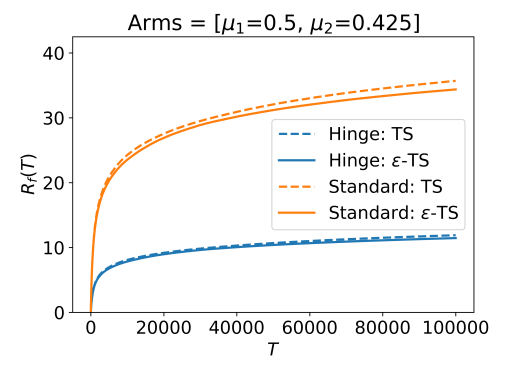
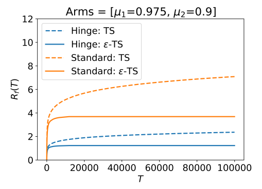
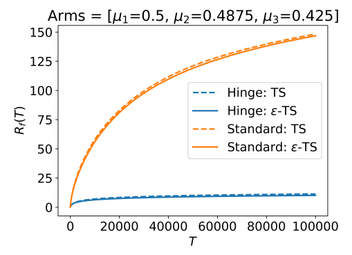
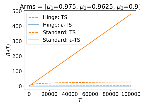
Figure 4: Evaluation of $\epsilon$-TS and vanilla TS with $\epsilon=0.05$ and Bernoulli rewards. ‘Hinge’ is the $\epsilon$-gap function $f(\Delta)=\max\left\{\Delta-\epsilon,0\right\}$ and ‘Standard’ is the $0$-gap function $f(\Delta)=\Delta$, which leads to the standard regret.

F.3 Additional Experiments

In this subsection, we present additional experiments that were omitted from the paper due to space limits. All simulations were done with $\epsilon=0.2$. In Figure 5(a) and Figure 5(b) we simulated edge cases that were omitted due to the similarity to the simulations in Figure 3. In Figure 5(a), we simulate the transition point where $\mu^{*}=1-\epsilon$. Notably, we observe that in this case, the simulation behaves very similarly to the case where $\mu^{*}>1-\epsilon$. In Figure 5(a), we study the case where $\mu_{2}$ is slightly below $\mu_{1}-\epsilon$. As expected, the behavior is very similar to the case where $\mu_{2}<\mu_{1}-\epsilon$ and the gap is larger, with the only difference that the hinge-loss is smaller. Next, in Figure 5(c), we present a longer version of the bottom-left experiment in Figure 3, where $\epsilon$-TS surpasses TS also in terms of the standard regret. When running a longer experiment, we see that this continues until the $20,000^{th}$ step, and then TS achieves lower regret. We believe that this is since $\epsilon$-TS gives less focus to arm $a_{3}$, but still has a good chance for identifying that $a_{1}$ is optimal. Then, it takes many steps until the possible mistakes of $\epsilon$-TS in identifying $a_{1}$ are more harmful than the exploration of $a_{3}$ by TS. Finally, we simulated a problem with 20 randomly-generated arms as follows: the optimal arm was selected to $\mu^{*}=0.6$. Then, 9 arms were uniformly generated in $\left[0.4,0.6\right]$ and 10 arms were generated in $\left[0,0.4\right]$. The resulting arms are presented in Table 3. These arms were then fixed, and we simulated the lenient regret for $1,000$ seeds. The results of this simulation are in Figure 5(d). Interestingly, we see a similar phenomena to that of Figure 5(c) – even after $100,000$ steps, $\epsilon$-TS enjoys better standard regret than $TS$. Both simulations hint that for short horizons, $\epsilon$-TS achieves better performance than the vanilla TS, and we believe it is interesting to further study the performance of $\epsilon$-TS in short horizons. Finally, we supply additional statistics on the simulations in Table 4.

Table 3: Arm values in Figure 5(d), sorted in an increasing order

0.153	0.169	0.175	0.218	0.22	0.241	0.258	0.286	0.357	0.385
0.404	0.414	0.417	0.506	0.514	0.55	0.558	0.567	0.585	0.6

Table 4: Additional statistics of the empirical evaluation in Figure 5. The statistics are calculated at the end of the run and are as in Table 1.

		Thompson sampling				$\epsilon$-Thompson sampling
Scenario	Regret Type	mean	std	$99\%$	max	mean	std	$99\%$	max
	Standard	6.88	4.57	20.4	280.2	2.99	12.7	26.1	1344.9
Figure 5(a)	Hinge	2.3	1.52	6.8	93.4	1	4.23	8.7	448.3
	Standard	10.69	7.48	30.66	549.15	7.66	13.68	34.02	1046.64
Figure 5(b)	Hinge	0.51	0.36	1.46	26.15	0.36	0.65	1.62	49.84
	Standard	59.55	50.16	164.55	1550.35	71.34	322.73	597.33	5017.9
Figure 5(c)	Hinge	4.08	1.6	8.6	11.6	2.58	1.23	6.3	10
	Standard	472.64	165.14	1110.64	1948.38	331.02	272.78	1739.39	2060.39
Figure 5(d)	Hinge	42.26	5.24	55.57	58.48	24.31	3.78	34.91	38.54

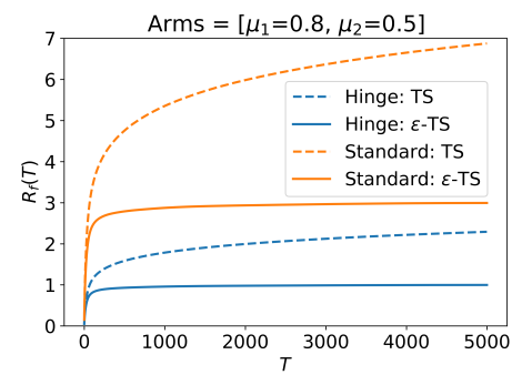
(a) 50,000 seeds, $\mu^{*}=1-\epsilon$

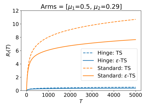
(b) 50,000 seeds, $\mu_{2}$ just below $\mu^{*}-\epsilon$

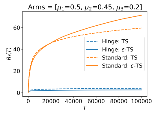
(c) 5,000 seeds, longer horizon for the experiment in Figure 3

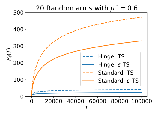
(d) 1,000 seeds, 20 random arms that were generated once with $\mu^{*}=0.6$

Figure 5: Evaluation of $\epsilon$-TS and vanilla TS with $\epsilon=0.2$ and Bernoulli rewards.‘Hinge’ is the $\epsilon$-gap function $f(\Delta)=\max\left\{\Delta-\epsilon,0\right\}$ and ‘Standard’ is the $0$-gap function $f(\Delta)=\Delta$, which leads to the standard regret.

References

- Agrawal and Goyal [2012] Shipra Agrawal and Navin Goyal. Analysis of thompson sampling for the multi-armed bandit problem. In Conference on learning theory, pages 39–1, 2012.
- Agrawal and Goyal [2013a] Shipra Agrawal and Navin Goyal. Further optimal regret bounds for thompson sampling. In Artificial intelligence and statistics, pages 99–107, 2013a.
- Agrawal and Goyal [2013b] Shipra Agrawal and Navin Goyal. Thompson sampling for contextual bandits with linear payoffs. In International Conference on Machine Learning, pages 127–135, 2013b.
- Auer et al. [2002] Peter Auer, Nicolo Cesa-Bianchi, and Paul Fischer. Finite-time analysis of the multiarmed bandit problem. Machine learning, 47(2-3):235–256, 2002.
- Bubeck et al. [2012] Sébastien Bubeck, Nicolo Cesa-Bianchi, et al. Regret analysis of stochastic and nonstochastic multi-armed bandit problems. Foundations and Trends® in Machine Learning, 5(1):1–122, 2012.
- Bubeck et al. [2013] Sébastien Bubeck, Vianney Perchet, and Philippe Rigollet. Bounded regret in stochastic multi-armed bandits. In Conference on Learning Theory, pages 122–134, 2013.
- Burnetas and Katehakis [1996] Apostolos N Burnetas and Michael N Katehakis. Optimal adaptive policies for sequential allocation problems. Advances in Applied Mathematics, 17(2):122–142, 1996.
- Chapelle and Li [2011] Olivier Chapelle and Lihong Li. An empirical evaluation of thompson sampling. In Advances in neural information processing systems, pages 2249–2257, 2011.
- Chaudhuri and Kalyanakrishnan [2017] Arghya Roy Chaudhuri and Shivaram Kalyanakrishnan. Pac identification of a bandit arm relative to a reward quantile. In AAAI, volume 17, pages 1977–1985, 2017.
- Chen et al. [2016a] Wei Chen, Yajun Wang, Yang Yuan, and Qinshi Wang. Combinatorial multi-armed bandit and its extension to probabilistically triggered arms. The Journal of Machine Learning Research, 17(1):1746–1778, 2016a.
- Dann and Brunskill [2015] Christoph Dann and Emma Brunskill. Sample complexity of episodic fixed-horizon reinforcement learning. In Advances in Neural Information Processing Systems, pages 2818–2826, 2015.
- Dann et al. [2017] Christoph Dann, Tor Lattimore, and Emma Brunskill. Unifying pac and regret: Uniform pac bounds for episodic reinforcement learning. In Advances in Neural Information Processing Systems, pages 5713–5723, 2017.
- Even-Dar et al. [2002] Eyal Even-Dar, Shie Mannor, and Yishay Mansour. Pac bounds for multi-armed bandit and markov decision processes. In International Conference on Computational Learning Theory, pages 255–270. Springer, 2002.
- Gabillon et al. [2012] Victor Gabillon, Mohammad Ghavamzadeh, and Alessandro Lazaric. Best arm identification: A unified approach to fixed budget and fixed confidence. In Advances in Neural Information Processing Systems, pages 3212–3220, 2012.
- Garivier and Cappé [2011] Aurélien Garivier and Olivier Cappé. The kl-ucb algorithm for bounded stochastic bandits and beyond. In Proceedings of the 24th annual conference on learning theory, pages 359–376, 2011.
- Garivier et al. [2019] Aurélien Garivier, Pierre Ménard, and Gilles Stoltz. Explore first, exploit next: The true shape of regret in bandit problems. Mathematics of Operations Research, 44(2):377–399, 2019.
- Kakade et al. [2003] Sham Machandranath Kakade et al. On the sample complexity of reinforcement learning. PhD thesis, University of London London, England, 2003.
- Kano et al. [2019] Hideaki Kano, Junya Honda, Kentaro Sakamaki, Kentaro Matsuura, Atsuyoshi Nakamura, and Masashi Sugiyama. Good arm identification via bandit feedback. Machine Learning, 108(5):721–745, 2019.
- Kaufmann et al. [2012] Emilie Kaufmann, Nathaniel Korda, and Rémi Munos. Thompson sampling: An asymptotically optimal finite-time analysis. In International conference on algorithmic learning theory, pages 199–213. Springer, 2012.
- Korda et al. [2013] Nathaniel Korda, Emilie Kaufmann, and Remi Munos. Thompson sampling for 1-dimensional exponential family bandits. In Advances in neural information processing systems, pages 1448–1456, 2013.
- Lai and Robbins [1985] Tze Leung Lai and Herbert Robbins. Asymptotically efficient adaptive allocation rules. Advances in applied mathematics, 6(1):4–22, 1985.
- Lattimore and Munos [2014] Tor Lattimore and Rémi Munos. Bounded regret for finite-armed structured bandits. In Advances in Neural Information Processing Systems, pages 550–558, 2014.
- Lattimore and Szepesvári [2018] Tor Lattimore and Csaba Szepesvári. Bandit algorithms. preprint, 2018.
- Lattimore et al. [2013] Tor Lattimore, Marcus Hutter, Peter Sunehag, et al. The sample-complexity of general reinforcement learning. In Proceedings of the 30th International Conference on Machine Learning. Journal of Machine Learning Research, 2013.
- Mannor and Tsitsiklis [2004] Shie Mannor and John N Tsitsiklis. The sample complexity of exploration in the multi-armed bandit problem. Journal of Machine Learning Research, 5(Jun):623–648, 2004.
- Robbins [1952] Herbert Robbins. Some aspects of the sequential design of experiments. Bulletin of the American Mathematical Society, 58(5):527–535, 1952.
- Russo and Van Roy [2016] Daniel Russo and Benjamin Van Roy. An information-theoretic analysis of thompson sampling. The Journal of Machine Learning Research, 17(1):2442–2471, 2016.
- Russo and Van Roy [2018] Daniel Russo and Benjamin Van Roy. Satisficing in time-sensitive bandit learning. arXiv preprint arXiv:1803.02855, 2018.
- Russo et al. [2018] Daniel J Russo, Benjamin Van Roy, Abbas Kazerouni, Ian Osband, and Zheng Wen. A tutorial on thompson sampling. Foundations and Trends® in Machine Learning, 11(1):1–96, 2018.
- Slivkins [2019] Aleksandrs Slivkins. Introduction to multi-armed bandits. arXiv preprint arXiv:1904.07272, 2019.
- Sutton and Barto [2018] Richard S Sutton and Andrew G Barto. Reinforcement learning: An introduction. MIT press, 2018.
- Thompson [1933] William R Thompson. On the likelihood that one unknown probability exceeds another in view of the evidence of two samples. Biometrika, 25(3/4):285–294, 1933.
- Trinh et al. [2019] Cindy Trinh, Emilie Kaufmann, Claire Vernade, and Richard Combes. Solving bernoulli rank-one bandits with unimodal thompson sampling. arXiv preprint arXiv:1912.03074, 2019.
- Wang and Chen [2018] Siwei Wang and Wei Chen. Thompson sampling for combinatorial semi-bandits. In International Conference on Machine Learning, pages 5114–5122, 2018.