Dielectric Laser Acceleration

Abstract

Dielectric Laser Accelerators (DLAs) use the nearfields created when a laser pulse impinges on a dielectric structure to accelerate charged particles. We provide an overview of the theory of operation of photon driven accelerators, from photons interacting with charged particles in a vacuum, to the advantages gained by introducing dielectric structures, with a discussion of their advantages and limitations. Furthermore we show the state of the art of the current development of dielectric laser accelerators, including acceleration, focusing, deflection, beam position monitoring, and advanced topics from the generation of microbunches to the adaptation of alternating phase focusing, allowing for the next to lossless transport of the charged particles over long distances.

1 Introduction

The idea of accelerators using dielectrics or stimulated emission to generate the necessary electromagnetic fields is not new. First proposals for such machines appeared in the 1970s. These consisted of maser pumped[Shimoda1962] accelerators — first demonstrated in 1987 using metallic gratings and mm wave radiation  [Mizuno1987], laser pumped metallic gratings  [Takeda1968] and finally laser pumped dielectric  [lohmann62, lohmann63] accelerators. The first successful demonstrations of what we now call dielectric laser accelerators happened in 2013, independently at relativistic electron velocities  [Peralta2013] and subrelativistic speeds  [Breuer]. Several advancements were necessary for a successful demonstration. Among others, the development of ultrashort laser pulses and their amplification — honoured with the 2018 Nobel prize in physics for the invention of chirped pulse amplification — to high peak intensities and the development of semiconductor technology that pressed forward the ability of manufacturing tiny devices on a scale of the wavelength used to drive these accelerators.

Although the use of metal gratings was demonstrated early on, maser or laser driven accelerators suffer the same drawbacks of a rather low damage threshold when using metallic materials as conventional radio frequency (RF) accelerators. Although damage mechanisms can vary from thermal to peak field driven effects metals, due to the availability of excitable electrons, the light can couple to the structure and cause damage. In dielectrics the bandgap provides transparency allowing refractive media to be used instead of metallic ones with much greater peak fields before damage is observed. This facilitates the generation of higher acceleration gradients compared to RF accelerators.
Due to the available laser sources that can provide short pulses and therefore sufficiently high peak fields and other considerations such as integrateability and wall plug power efficiency, the prefered wavelengths are usually below 2000nm. Therefore the structure features are roughly 1000nm and below. This miniaturization opens the door for applications other accelerator concepts are not capable of supplying medical irradiation in the body. This holds while DLAs currently require roughly an order of magnitude less power per meter of accelerator compared to Laser Plasma Wakefield Accelerators (LPWA). This has still great potential for improvement since most of the laser power is unused and can be recycled improving the DLAs efficiency in future devices.

2 Theory

2.1 Electromagnetic waves in vacuum

Starting from Maxwell’s equations, the feasibility of acceleration in vacuum, near dielectric boundaries and finally near microstructured dielectrics is explored, highlighting their respective advantages and limitations. In the following section we derive the wave nature of electro magnetic waves. Maxwell’s equations

$$\nabla\cdot\vec{E}=\frac{\rho}{\epsilon_{0}}$$ (1)

$$\nabla\cdot\vec{B}=0$$ (2)

$$\nabla\times\vec{E}=-\frac{\partial\vec{B}}{\partial t}$$ (3)

$$\nabla\times\vec{B}=\mu_{0}\epsilon_{0}\frac{\partial\vec{E}}{\partial t}+\mu_{0}\vec{J}$$ (4)

can be simplified with $\rho=0$ and $\vec{J}=0$ since all considerations are done in vacuum and therefore there are neither charges nor currents. Taking the curl of Faraday’s law of induction Eq. (3) changing the right hand side order of the differentiation yields

$$\nabla\times\left(\nabla\times\vec{E}\right)=-\frac{\partial}{\partial t}\left(\nabla\times\vec{B}\right).$$ (5)

Substituting Ampere’s law Eq. (4) and assuming that the vacuum permittivity $\epsilon_{0}$ and vacuum permeability $\mu_{0}$ are not time varying we arrive at

$$\nabla\times\left(\nabla\times\vec{E}\right)=-\mu_{0}\epsilon_{0}\frac{\partial^{2}\vec{E}}{\partial t^{2}}.$$ (6)

Using the identity $\nabla\times\left(\nabla\times\vec{A}\right)=\nabla\left(\nabla\cdot\vec{A}\right)-\nabla^{2}\vec{A}$ and Gauss’s law Eq. (1) yields the wave equation of the electric field

$$\nabla^{2}\vec{E}=\mu_{0}\epsilon_{0}\frac{\partial^{2}\vec{E}}{\partial t^{2}}.$$ (7)

Similar steps can be taken starting with Ampere’s law to arrive at the analogous wave equation for the magnetic field

$$\nabla^{2}\vec{B}=\mu_{0}\epsilon_{0}\frac{\partial^{2}\vec{B}}{\partial t^{2}}.$$ (8)

The easiest solution for these wave equations are the plane waves:

$$\vec{E}\left(t,\vec{r}\right)=E_{0}\cdot e^{i\vec{k}\vec{r}-i\omega t}\;\;\;\text{and}\;\;\;\vec{B}\left(t,\vec{r}\right)=B_{0}\cdot e^{i\vec{k}\vec{r}-i\omega t}.$$ (9)

2.2 Acceleration without dielectrics

Interaction between a single plane wave and a charged particle only affects the particles momentum during the interaction. After the interaction, averaging over the electromagnetic field, the particles momentum is unchanged. This is due to the conservation of energy and momentum, sometimes referred to as the Lawson-Woodward theorem for the seven cases Lawson and Woodward postulated under which, if all are satisfied, no net acceleration can take place.
One of the seven rules states that nonlinear forces must be neglected. By utilizing nonlinear forces, acceleration without any structures becomes possible. One such force is the ponderomotive force

$$\vec{F}_{p}=-\frac{e^{2}}{4m\omega^{2}}\nabla E^{2}.$$ (10)

It is dependent on the square of the electric field and has the effect of pushing particles from high intensity regions to low intensity regions[Kozak2018a]. By utilizing two or more intersecting laser fields, a travelling interference pattern can be created that is co-propagating with electrons. The properties of this travelling wave, its velocity, are set by the intersecting waves’ wavelengths and intersecting angles. By adjusting the mode velocity to the electron velocity, synchronous interaction between the light wave and the electrons can be achieved. One definite advantage of this approach is that due to the absence of any medium, the peak intensity used can be easily increased without damaging structures, however scalability of the interaction distance is not trivial and due to the nonlinear nature of the interaction large pulse energies are required to generate the large peak fields necessary.

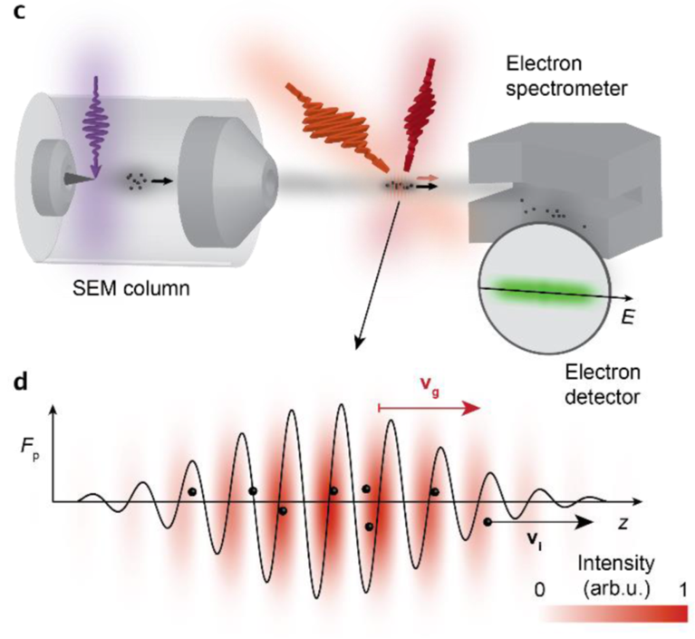
Figure 1: Setup to generate a travelling wave to change influence the electrons momenta (top) Ponderomotive wave with group velocity $v_{g}$ synchronous to the electron velocity. Electrons experience a force according to the gradient from high intensity to low intensity. Electrons on the right hand side of a high intensity region get accelerated, where as electrons on the left side get decelerated. (bottom)

2.3 Acceleration close to a dielectric interface

Placing a dielectric close to the particle beam can alleviate some of the shortcomings of the ponderomotive method. By evaluating the electromagnetic fields in an infinitesimally small area or loop across a boundary, we can arrive at the continuity conditions

$$n_{12}\times\left(\vec{E_{2}}-\vec{E_{1}}\right)=0$$ (11)

$$\left(\vec{D_{2}}-\vec{D_{1}}\right)\cdot n_{12}=\sigma_{s}$$ (12)

$$\left(\vec{B_{2}}-\vec{B_{1}}\right)\cdot n_{12}=0$$ (13)

$$n_{12}\times\left(\vec{H_{2}}-\vec{H_{1}}\right)=\vec{j_{s}},$$ (14)

with $n_{12}$ the normal vector of the interface, $\sigma_{s}$ the surface charge and $\vec{j_{s}}thesurfacecurrent$ – which both are zero due to only considering dielectrics. From these equations we see that the tangential part of the electric field $\vec{E}$ and the magnetic field strength $\vec{H}$ have to be continuous across the interface. Furthermore, the normal components of the electric displacement field $\vec{D}$ and the magnetic field $\vec{B}$ have to be continuous.
Finally, when evaluating these boundary conditions together with the plane waves, we arrive at certain conditions the incident, transmitted and reflected waves have to satisfy. In Fig. LABEL:fig:waves a) we see the incident and transmitted wave at an interface. From

$$\left(\vec{k_{i}}-\vec{k_{r}}\right)\cdot\vec{r}=0\;\;\;and\;\;\;\left(\vec{k_{i}}-\vec{k_{t}}\right)\cdot\vec{r}=0$$ (15)

we see that the x component of the wave vector, parallel to the materials interface, needs to have the same value in all three waves $k_{i,x}=k_{r,x}=k_{t,x}$. We use

$$k_{i,x}=\lvert\vec{k_{i}}\rvert\sin{\phi}=\frac{n_{i}\omega}{c}\sin{\phi},$$ (16)

with the dispersion relation $k=\frac{n\omega}{c}$ and the incident angle $\phi$. Similarly we decompose the transmitted wave:

$$\lvert\vec{k_{t}}\rvert=\frac{n_{t}\omega}{c}=\sqrt{k^{2}_{t,x}+k^{2}_{t,y}}$$ (17)

Finally we use that $k^{2}_{t,x}=k^{2}_{i,x}$ to solve for $k_{t,y}$