Intelligent Matrix Exponentiation

Abstract

We present a novel machine learning architecture that uses the exponential of a single input-dependent matrix as its only nonlinearity. The mathematical simplicity of this architecture allows a detailed analysis of its behaviour, providing robustness guarantees via Lipschitz bounds. Despite its simplicity, a single matrix exponential layer already provides universal approximation properties and can learn fundamental functions of the input, such as periodic functions or multivariate polynomials. This architecture outperforms other general-purpose architectures on benchmark problems, including CIFAR-10, using substantially fewer parameters.

Google Research
Brandschenkestrasse 110, 8002 Zürich, Switzerland
{tfish,iuliacomsa,dickstra,firsching,veluca,jyrki}@google.com

1 Introduction

Deep neural networks (DNNs) synthesize highly complex functions by composing a large number of neuronal units, each featuring a basic and usually $1$-dimensional nonlinear activation function $f:\mathbb{R}^{1}\to\mathbb{R}^{1}$. While highly successful in practice, this approach also has disadvantages. In a conventional DNN, any two activations only ever get combined through summation. This means that such a network requires an increasing number of parameters to express more complex functions even as simple as multiplication. This approach of composing simple functions does not generalize well outside the boundaries of the training data.

An alternative to the composition of many 1-dimensional functions is using a simple higher-dimensional nonlinear function $f:\mathbb{R}^{m}\to\mathbb{R}^{n}$. A single multidimensional nonlinearity may be desirable because it could express more complex relationships between input features with potentially fewer parameters and fewer mathematical operations.

The matrix exponential stands out as a promising but overlooked candidate for a higher-dimensional nonlinearity that may be used as a building block for machine learning models. The matrix exponential is a smooth function governed by a relatively simple equation that yields desirable mathematical properties. It has applications in solving linear differential equations and plays a prominent role in the theory of Lie groups, an algebraic structure widely used throughout many branches of mathematics and science.

We propose a novel ML architecture for supervised learning whose core element is a single layer (henceforth referred to as “M-layer”), that computes a single matrix exponential, where the matrix to be exponentiated is an affine function of the input features. We show that the M-layer has universal approximator properties and allows closed-form per-example bounds for robustness. We demonstrate the ability of this architecture to learn multivariate polynomials, such as matrix determinants, and to generalize periodic functions beyond the domain of the input without any feature engineering. Furthermore, the M-layer achieves results comparable to recently-proposed non-specialized architectures on image recognition datasets. We provide open-source TensorFlow code that implements the M-layer: https://github.com/google-research/google-research/tree/master/m_layer.

2 Related Work

Neuronal units with more complex activation functions have been proposed. One such example are sigma-pi units [RHM86], whose activation function is the weighted sum of products of its inputs. More recently, neural arithmetic logic units have been introduced [THR⁺18], which can combine inputs using multiple arithmetic operators and generalize outside the domain of the training data. In contrast with these architectures, the M-layer is not based on neuronal units with multiple inputs, but uses a single matrix exponential as its nonlinear mapping function. Through the matrix exponential, the M-layer can easily learn mathematical operations more complex than addition, but with simpler architecture. In fact, as shown in Section 3.3, the M-layer can be regarded as a generalized sigma-pi network with built-in architecture search, in the sense that it learns by itself which arithmetic graph should be used for the computation.

Architectures with higher-dimensional nonlinearities are also already used. The softmax function is an example for a widely-used such nonlinear activation function that solves a specific problem, typically in the final layer of classifiers. Like the M-layer, it has extra mathematical structure. For example, a permutation of the softmax inputs produces a corresponding permutation of the outputs. Maxout networks also act on multiple units and have been successful in combination with dropout [GWFM⁺13]. In radial basis networks [PS91], each hidden unit computes a nonlinear function of the distance between its own learned centroid and a single point represented by a vector of input coordinates. Capsule networks [SFH17] are another recent example of multidimensional nonlinearities. Similarly, the M-layer uses the matrix exponential as a single high-dimensional nonlinearity, therefore creating additional mathematical structure that potentially allows solving problems using fewer parameters than compositional architectures.

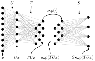
Figure 1: Schematic diagram of the M-layer architecture.

Matrix exponentiation has a natural alternative interpretation in terms of an ordinary differential equation (ODE). As such, the M-layer can be compared to other novel ODE-related architectures that have been proposed recently. In particular, neural ordinary differential equations (NODE) [CRBD18] and their augmented extensions (ANODE) [DDT19] have recently received attention. We discuss this in Section 3.6.

Existing approaches to certifying the robustness of neural networks can be split into two different categories. Some approaches [PRGS17] mathematically analyze a network layer by layer, providing bounds on the robustness of each layer, that then get multiplied together. This kind of approach tends to give fairly loose bounds, due to the inherent tightness loss from composing upper bounds. Other approaches [SGPV18, SGPV19] use abstract interpretation on the evaluation of the network to provide empirical robustness bounds. In contrast, using the fact that the M-layer architecture has a single layer, in Section 3.7 we obtain a direct bound on the robustness on the whole network by analyzing the explicit formulation of the computation.

3 Architecture

We start this section by refreshing the definition of the matrix exponential. We then define the proposed M-layer model and explain its ability to learn particular functions such as polynomials and periodic functions. Finally, we provide closed-form per-example robustness guarantees.

3.1 Matrix Exponentiation

The exponential of a square matrix $M$ is defined as:

$$\exp(M)=\sum_{k=0}^{\infty}\frac{1}{k!}M^{k}$$ (1)

The matrix power $M^{k}$ is defined inductively as ${M^{0}=I}$, ${M^{k+1}=M\cdot M^{k}}$, using the associativity of the matrix product; it is not an element-wise matrix operation.

Note that the expansion of $\exp(M)$ in Eq. (1) is finite for nilpotent matrices. A matrix $M$ is called nilpotent if there exists a positive integer $k$ such that $M^{k}=0$. Strictly upper triangular matrices are a canonical example.

Multiple algorithms for computing the matrix exponential efficiently have been proposed [MV03]. TensorFlow implements tf.linalg.expm using the scaling and squaring method combined with the Padé approximation [Hig05].

3.2 M-Layer Definition

At the core of the proposed architecture is an M-layer that computes a single matrix exponential, where the matrix to be exponentiated is an affine function of all of the input features. In other words, an M-layer replaces an entire stack of hidden layers in a DNN.

Figure 1 shows a diagram of the proposed architecture. We exemplify the architecture as applied to a standard image recognition dataset, but we note that this formulation is applicable to any other type of problem by adapting the relevant input indices. In the following equations, generalized Einstein summation is performed over all right-hand side indices not seen on the left-hand side. This operation is implemented in TensorFlow by tf.einsum.

Consider an example input image, encoded as a $3$-index array $X_{yxc}$, where $y$, $x$ and $c$ are the row index, column index and color channel index, respectively. The matrix $M$ to be exponentiated is obtained as follows, using the trainable parameters $\tilde{T}_{ajk}$, $\tilde{U}_{axyc}$ and $\tilde{B}_{jk}$:

$$M=\tilde{B}_{jk}+\tilde{T}_{ajk}\tilde{U}_{ayxc}X_{yxc}$$ (2)

$X$ is first projected linearly to a $d$-dimensional latent feature embedding space by $\tilde{U}_{ayxc}$. Then, the $3$-index tensor $\tilde{T}_{ajk}$ maps each such latent feature to an $n\times n$ matrix. Finally, a bias matrix $\tilde{B}_{jk}$ is added to the feature-weighted sum of matrices. The result is a matrix indexed by row and column indices $j$ and $k$.

We remark that it is possible to contract the tensors $\tilde{T}$ and $\tilde{U}$ in order to simplify the architecture formula, but partial tensor factorization provides regularization by reducing the parameter count.

An output $p_{m}$ is obtained as follows, using the trainable parameters $\tilde{S}_{mjk}$ and $\tilde{V}_{m}$:

$$p_{m}=\tilde{V}_{m}+\tilde{S}_{mjk}\exp(M)_{jk}$$ (3)

The matrix $\exp(M)$, indexed by row and column indices $j$ and $k$ in the same way as $M$, is projected linearly by the $3$-index tensor $\tilde{S}_{mjk}$, to obtain a $h$-dimensional output vector. The bias-vector $\tilde{V}_{m}$ turns this linear mapping into an affine mapping. The resulting vector may be interpreted as accumulated per-class evidence and, if desired, may then be mapped to a vector of probabilities via softmax.

Training is done conventionally, by minimizing a loss function such as the $L_{2}$ norm or the cross-entropy with softmax, using backpropagation through matrix exponentiation.

The nonlinearity of the M-layer architecture is provided by the $\mathbb{R}^{d}\to\mathbb{R}^{h}$ mapping $v\mapsto\tilde{V}_{m}+\tilde{S}_{mjk}\exp(M)_{jk}$. The count of trainable parameters of this component is $dn^{2}+n^{2}+n^{2}h+h$. This count comes from summing the dimensions of $\tilde{T}_{ajk}$, $\tilde{B}_{jk}$, $\tilde{S}_{mjk}$, and $\tilde{V}_{m}$, respectively. We note that this architecture has some redundancy in its parameters, as one can freely multiply the $T$ and $U$ tensors by a $d\times d$ real matrix and, respectively, its inverse, while preserving the computed function. Similarly, it is possible to multiply each of the $n\times n$ parts of the tensors $\tilde{T}$ and $\tilde{S}$, as well as $B$, by both an $n\times n$ matrix and its inverse. In other words, any pair of real invertible matrices of sizes $d\times d$ and $n\times n$ can be used to produce a new parametrization that still computes the same function.

3.3 Feature Crosses and Universal Approximation

A key property of the M-layer is its ability to generate arbitrary exponential-polynomial combinations of the input features. For classification problems, M-layer architectures are a superset of multivariate polynomial classifiers, where the matrix size constrains the complexity of the polynomial while at the same time not uniformly constraining its degree. In other words, simple multivariate polynomials of high degree compete against complex multivariate polynomials of low degree.

We provide a universal approximator proof for the M-layer in the Supplementary Material, which relies on its ability to express any multivariate polynomial in the input features if a sufficiently large matrix size is used. We provide here an example that illustrates how feature crosses can be generated through the matrix exponential.

Consider a dataset with the feature vector $(\phi_{0},\phi_{1},\phi_{2})$ given by the $\tilde{U}\cdot x$ tensor contraction, where the relevant quantities for the final classification of an example are assumed to be $\phi_{0}$, $\phi_{1}$, $\phi_{2}$, $\phi_{0}\phi_{1}$, and $\phi_{1}\phi_{2}^{2}$. To learn this dataset, we look for an exponentiated matrix that makes precisely these quantities available to be weighted by the trainable tensor $\tilde{S}$. To do this, we define three $7\times 7$ matrices $T_{0jk}$, $T_{1jk}$, and $T_{2jk}$ as $T_{001}=T_{102}=T_{203}=1$, $T_{024}=T_{225}=2$, $T_{256}=3$, and $0$ otherwise. We then define the matrix $M$ as:

$$M=\phi_{0}T_{0}+\phi_{1}T_{1}+\phi_{2}T_{2}=\left(\begin{smallmatrix}0&\phi_{0}&\phi_{1}&\phi_{2}&0&0&0\\ 0&0&0&0&0&0&0\\ 0&0&0&0&2\phi_{0}&2\phi_{2}&0\\ 0&0&0&0&0&0&0\\ 0&0&0&0&0&0&0\\ 0&0&0&0&0&0&3\phi_{2}\\ 0&0&0&0&0&0&0\end{smallmatrix}\right)$$

Note that $M$ is nilpotent, as $M^{4}=0$. Therefore, we obtain the following matrix exponential, which contains the desired quantities in its leading row:

$$\exp(M) =I+M+\frac{1}{2}M^{2}+\frac{1}{6}M^{3}=$$

$$=\left(\begin{smallmatrix}1&\phi_{0}&\phi_{1}&\phi_{2}&\phi_{0}\phi_{1}&\phi_{1}\phi_{2}&\phi_{1}\phi_{2}^{2}\\ 0&1&0&0&0&0&0\\ 0&0&1&0&2\phi_{0}&2\phi_{2}&3\phi_{2}^{2}\\ 0&0&0&1&0&0&0\\ 0&0&0&0&1&0&0\\ 0&0&0&0&0&1&3\phi_{2}\\ 0&0&0&0&0&0&1\end{smallmatrix}\right)$$

The same technique can be employed to encode any polynomial in the input features using a $n\times n$ matrix, where $n$ is one unit larger than the total number of features plus the intermediate and final products that need to be computed. The matrix size can be seen as regulating the total capacity of the model for computing different feature crosses.

With this intuition, one can read the matrix as a “circuit breadboard” for wiring up arbitrary polynomials. When evaluated on features that only take values $0$ and $1$, any Boolean logic function can be expressed.

3.4 Feature Periodicity

While the M-layer is able to express a wide range of functions using the exponential of nilpotent matrices, non-nilpotent matrices can bring additional utility. One possible application of non-nilpotent matrices is learning the periodicity of input features. This is a problem where conventional DNNs struggle, as they cannot naturally generalize beyond the distribution of the training data. Here we illustrate how matrix exponentials can naturally fit periodic dependency on input features, without requiring an explicit specification of the periodic nature of the data.

Consider the matrix $M_{r}=\left(\begin{smallmatrix}0&-\omega\\ \omega&0\end{smallmatrix}\right)$. We have $\exp(tM_{r})=\left(\begin{smallmatrix}\cos\omega t&-\sin\omega t\\ \sin\omega t&\phantom{+}\cos\omega t\end{smallmatrix}\right)$, which is a 2d rotation by an angle of $\omega t$ and thus periodic in $t$ with period $2\pi/\omega$. This setup can fit functions that have an arbitrary period. Moreover, this representation of periodicity naturally extrapolates well when going beyond the range of the initial numerical data.

3.5 Connection to Lie Groups

The M-layer has a natural connection to Lie groups. Lie groups can be thought of as a model of continuous symmetries of a system such as rotations. There is a large body of mathematical theory and tools available to study the structure and properties of Lie groups [Gil08, Gil12], which may ultimately also help for model interpretability.

Every Lie group has associated a Lie algebra, which can be understood as the space of the small perturbations with which it is possible to generate the elements of the Lie group. As an example, the set of rotations of $3$-dimensional space forms a Lie group; the corresponding algebra can be understood as the set of rotation axes in $3$ dimensions. Lie groups and algebras can be represented using matrices, and by computing a matrix exponential one can map elements of the algebra to elements of the group.

In the M-layer architecture, the role of the $3$-index tensor $\tilde{T}$ is to form a matrix whose entries are affine functions of the input features. The matrices that compose $\tilde{T}$ can be thought of as generators of a Lie algebra. Building $M$ corresponds to selecting a Lie algebra element. Matrix exponentiation then computes the corresponding Lie group element.

As rotations are periodic and one of the simplest forms of continuous symmetries, this perspective is useful for understanding the ability of the M-layer to learn periodicity in input features.

3.6 Dynamical Systems Interpretation

Recent work has proposed a dynamical systems interpretation of some DNN architectures. The NODE architecture [CRBD18] uses a nonlinear and not time-invariant ODE that is provided by trainable neural units, and computes the time evolution of a vector that is constructed from the input features. This section discusses a similar interpretation of the M-layer.

Consider an M-layer with $\tilde{T}$ defined as $\tilde{T}_{012}=\tilde{T}_{120}=\tilde{T}_{201}=+1$, $\tilde{T}_{210}=\tilde{T}_{102}=\tilde{T}_{021}=-1$, and $0$ otherwise, with $\tilde{U}$ as the $3\times 3$ identity matrix, and with $\tilde{B}=0$. Given an input vector $a$, the corresponding matrix $M$ is then $\left(\begin{smallmatrix}0&a_{2}&-a_{1}\\ -a_{2}&0&a_{0}\\ a_{1}&-a_{0}&0\\ \end{smallmatrix}\right)$. Plugging $M$ into the linear and time invariant (LTI) ODE $d/dt\,Y(t)=MY(t)$, we can observe that the ODE describes a rotation around the axis defined by $a$. Moreover, a solution to this ODE is given by $Y(t)=\exp(tM)Y(0)$. Thus, by choosing $S_{mjk}=Y(0)_{k}$ if $m=j$ and $0$ otherwise, the above M-layer can be understood as applying a rotation with input dependent angular velocity to some basis vector over a unit time interval.

More generally, we can consider the input features to provide affine parameters that define a time-invariant linear ODE, and the output of the M-layer to be an affine function of a vector that has evolved under the ODE over a unit time interval. In contrast, the NODE architecture uses a non-linear ODE that is not input dependent, which gets applied to an input-dependent feature vector.

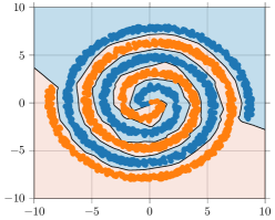
(a) ReLU

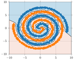
(b) tanh

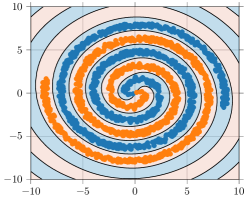
(c) M-layer

Figure 2: Comparison of ReLU/tanh DNN and M-layer classification boundaries on a double spiral (“Swiss roll”) classification task.

3.7 Certified Robustness

We show that the mathematical structure of the M-layer allows a novel proof technique to produce closed-form expressions for guaranteed robustness bounds.

For any matrix norm $\lVert\cdot\rVert$, we have [RC94]:

$$\lVert\exp(X+Y)-\exp(X)\rVert\leq\lVert Y\rVert\exp(\lVert Y\rVert)\exp(\lVert X\rVert)$$

We also make use of the fact that $\lVert M\rVert_{F}\leq\sqrt{n}\lVert M\rVert_{2}$ for any $n\times n$ matrix, where $\lVert\cdot\rVert_{F}$ is the Frobenius norm and $\lVert\cdot\rVert_{2}$ is the $2$-norm of a matrix. We recall that the Frobenius norm of a matrix is equivalent to the $2$-norm of the vector formed from the matrix entries.

Let $M$ be the matrix to be exponentiated corresponding to a given input example $x$, and let $M^{\prime}$ be the deviation to this matrix that corresponds to an input deviation of $\tilde{x}$, i.e. $M+M^{\prime}$ is the matrix corresponding to input example $x+\tilde{x}$. Given that the mapping between $x$ and $M$ is linear, there is a per-model constant $\delta_{in}$ such that $\lVert M^{\prime}\rVert_{2}\leq\delta_{in}\lVert\tilde{x}\rVert_{\infty}$.

The $2$-norm of the difference between the outputs can be bound as follows:

$$\lVert\Delta_{o}\rVert_{2} \leq \lVert S\rVert_{2}\lVert\exp(M+M^{\prime})-\exp(M)\rVert_{F}\leq$$

$$\leq \sqrt{n}\lVert S\rVert_{2}\lVert\exp(M+M^{\prime})-\exp(M)\rVert_{2}\leq$$

$$\leq \sqrt{n}\lVert S\rVert_{2}\lVert M^{\prime}\rVert_{2}\exp(\lVert M^{\prime}\rVert_{2})\exp(\lVert M\rVert_{2})\leq$$

$$\leq \sqrt{n}\lVert S\rVert_{2}\delta_{in}\lVert\tilde{x}\rVert_{\infty}\exp(\delta_{in}\lVert\tilde{x}\rVert_{\infty})\exp(\lVert M\rVert_{2})$$

where $\lVert S\rVert_{2}$ is computed by considering $S$ a $h\times n\cdot n$ rectangular matrix, and the first inequality follows from the fact that the tensor multiplication by $S$ can be considered a matrix-vector multiplication between $S$ and the result of matrix exponential seen as a $n\cdot n$ vector.

This inequality allows to compute the minimal $L_{\infty}$ change required in the input given the difference between the amount of accumulated evidence between the most likely class and other classes. Moreover, considering that $\lVert x\rVert_{\infty}$ is bounded from above, for example by $1$ in the case of CIFAR-10, we can obtain a Lipschitz bound by replacing the $\exp(\delta_{in}\lVert\tilde{x}\rVert_{\infty})$ term with a $\exp(\delta_{in})$ term.

4 Results

In this section, we demonstrate the performance of the M-layer on multiple benchmark tasks, in comparison with more traditional architectures. We first investigate the shape of the classification boundaries in a classic double spiral problem. We then show that the M-layer is able to learn determinants of matrices up to size $5\times 5$, periodic functions in the presence of low noise, and image recognition datasets at a level competitive with other non-specialized architectures. For CIFAR-10, we compare the training times and robustness to those of traditional DNNs.

The following applies for all experiments below, unless otherwise stated. DNN models are initialized using uniform Glorot initialization [GB10], while M-layer models are initialized with normally distributed values with mean $0$ and $\sigma=0.05$. To enhance training stability and model performance, an activity regularization is performed on the output of the M-layer. This is achieved by adding $\lambda\lVert\exp(M)\rVert^{2}_{F}$ to the loss function with a value of $\lambda$ equal to $10^{-4}$. This value is chosen because it performs best on the CIFAR-10 dataset from a choice of $10^{-3}$, $5\cdot 10^{-3}$, $10^{-4}$, $5\cdot 10^{-4}$, and $5\cdot 10^{-5}$.

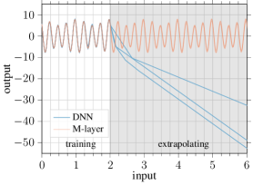
(a)

$1.42\cos(6\pi x+0.84)+6.29\cos(8\pi x+0.76)$

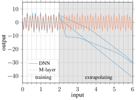
(b)

$1.55\cos(8\pi x+0.26)+5.07\cos(14\pi x+0.81)$

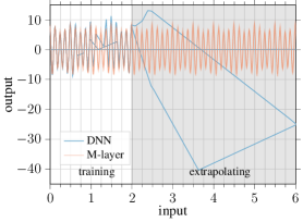
(c)

$1.60\cos(12\pi x+0.59)+6.92\cos(16\pi x+0.44)$

Figure 3: Learning periodic functions with a DNN and an M-layer. Each plot shows outputs from three separate models of each type.

4.1 Learning Double Spirals

To compare the classification boundaries generated by the M-layer with those of more traditional architectures, we train DNNs with ReLU and tanh activation functions, as well as M-layers, using a double spiral (“Swiss roll”) classification task as a toy problem.

The data consist of $2000$ randomly generated points along two spirals, with coordinates in the $[-10,10]$ range. Uniform random noise in the $[-0.5,0.5]$ range is added to each input coordinate. As we are only interested in the classification boundaries, no test or validation set is used.

The M-layer has a representation size $d=10$ and a matrix size $n=1$. Each DNN has two hidden layers of size $20$.

A RMSprop optimizer is used to minimize the cross-entropy with softmax. The M-layer is trained for $100$ epochs using a learning rate of $0.001$. The ReLU DNN is trained for $1000$ epochs using a learning rate of $0.001$. The tanh DNN is trained for $1000$ epochs using a learning rate of $0.01$. These values are chosen in such a way that all networks achieved a perfect fit.

The resulting boundaries for the three models are shown in Figure 2. They illustrate the distinctive ability of the M-layer to extrapolate functions beyond the training domain.

4.2 Learning Periodic Functions

To assess the capacity of the M-layer architecture to learn and extrapolate feature periodicity, we compare the performance of an M-layer and a DNN on periodic functions obtained as the sum of two cosines.

The data is generated as follows. The frequencies of the cosines are chosen as small integer multiples of $2\pi$ (from $3$ to $9$); the amplitudes are randomly generated from the intervals $[1,2]$ and $[5,10]$ respectively, and the phases are randomly generated in the $[0,\pi/3]$ range. Each model is trained on the $[0,2]$ range and tested it on the $[2,6]$ range, with a point spacing of $10^{-5}$. Gaussian random noise with $\sigma=10^{-4}$ is added to the target value of each training sample. No activity regularization is used.

The M-layer uses a representation size $d=1$ and a matrix size $n=6$, resulting in a trainable parameter count of $115$. Each cosine can be represented by using a $2$-dimensional subspace; a matrix size of $4$ would thus be sufficient, but $6$ was chosen to show that an M-layer can learn periodicity even when overparameterized.

In this experiment, the initialization of the bias and of $T_{0ij}$ is performed by generating normally distributed numbers with $\sigma=0.01$ and mean $-10$ for elements of the diagonal, and $0$ for all other elements. The coefficients of the mapping from input values to the embedding space are initialized with normally distributed values with mean $0.1$ and $\sigma=0.05$. This initialization is chosen in order to make it more likely for the initial matrix $M$ to be exponentiated to have negative eigenvalues and therefore keep outputs small.

The ReLU DNN is composed of two hidden layers with $50$ neurons each, followed by one hidden layer with $10$ neurons, resulting in a trainable parameter count of $3221$. The DNN was initialized using uniform Glorot initialization [GB10]. As the objective of this experiment is to demonstrate the ability to learn the periodicity of the input without additional engineering, we do not consider DNNs with special activation functions such as $\sin(x)$.

A RMSprop optimizer is used to minimize the following modified $L_{2}$ loss function: if $f$ is the function computed by the network, $x$ the input of the sample and $y$ the corresponding output, then the loss is given by $(f(x)-y)^{2}+\max(0,|f(2x+6)|-100)^{2}$. In other words, very large values in the $[6,10]$ time range are punished.

M-layers are trained for $300$ epochs with learning rate $5\cdot 10^{-3}$, decay rate $10^{-5}$ and batch size $128$. DNNs are trained for $300$ epochs with learning rate $10^{-3}$, decay rate $10^{-6}$ and batch size $64$. The hyperparameters are chosen by running multiple training steps with various choices of learning rate ($10^{-2}$, $10^{-3}$, $10^{-4}$), decay rate ($10^{-3}$, $10^{-4}$, $10^{-5}$, $10^{-6}$), batch size ($64$ and $128$) and number of epochs ($50$, $100$, $300$). For each model, the set of parameters that provided the best $L_{2}$ loss on the training set is chosen.

Examples of functions learned by the M-layer and the DNN are shown in Figure 3, which illustrates that, in contrast to the DNN, the M-layer is able to extrapolate such functions.

4.3 Learning Determinants

To demonstrate the ability of the M-layer to learn polynomials, we train an M-layer and a DNN to predict the determinant of $3\times 3$ and $5\times 5$ matrices. We do not explicitly encode any special property of the determinant, but rather employ it as an example multivariate polynomial that can be learnt by the M-layer. We confirm that we observe equivalent behavior for the matrix permanent.

Learning the determinant of a matrix with a small network is a challenging problem due to the size of its search space. A $5\times 5$ determinant is a polynomial with $120$ monomials of degree $5$ in $25$ variables. The generic inhomogeneous polynomial of this degree has ${25+5\choose 5}=142506$ monomials.

From Section 3.3, we know that it is possible to express this multivariate polynomial perfectly with a single M-layer. In fact, a strictly upper triangular and therefore nilpotent matrix can achieve this. We can use this fact to accelerate the learning of the determinant by masking out the lower triangular part of the matrix, but we do not pursue this idea here, as we want to demonstrate that an unconstrained M-layer is capable of learning polynomials as well.

The data consist of $n\times n$ matrices with entries sampled uniformly between $-1$ and $1$. With this sampling, the expected value of the square of the determinant is $\frac{n!}{3^{n}}$. So, we expect the square of the determinant to be $\frac{2}{9}$ for a $3\times 3$ matrix, and $\frac{40}{81}$ for a $5\times 5$ matrix. This means that an estimator constantly guessing $0$ would have a mean square error (MSE) of $\approx 0.2222$ and $\approx 0.4938$ for the two matrix sizes, respectively. This provides a baseline for the results, as a model that approximates the determinant function should yield a smaller error.

The size of the training set consists of between $2^{10}$ and $2^{17}$ examples for the $3\times 3$ matrices, and $2^{20}$ for the $5\times 5$ matrices. The validation set is $25\%$ of the training set size, in addition to it. Test sets consist of $10^{6}$ matrices.

The M-layer has $d=9$ and $n$ between $6$ and $12$ for $3\times 3$ determinants, and $n=24$ for $5\times 5$ determinants. The DNNs has $2$ to $4$ equally-sized hidden layers, each consisting of $5,10,15,20,25$ or $30$ neurons, for the $3\times 3$ matrices, and $5$ hidden layers of size $100$ for the $5\times 5$ matrices.

An RMSprop optimizer is used to minimize the MSE with an initial learning rate of $10^{-3}$, decay $10^{-6}$, and batch size $32$. These values are chosen to be in line with those chosen in Section 4.4. The learning rate is reduced by $80\%$ following $10$ epochs without validation accuracy improvement. Training is carried for a maximum of $256$ epochs, with early stopping after $30$ epochs without validation accuracy improvement.

Figure 4 shows the results of learning the determinant of $3\times 3$ matrices. The M-layer architecture is able to learn from fewer examples compared to the DNN. The best M-layer model learning on $2^{17}$ examples achieves a mean squared error of $\approx 2\cdot 10^{-4}$ with $811$ parameters, while the best DNN has a mean squared error of $\approx 0.003$ with $3121$ parameters.

Figure 5 shows the results of learning the determinant of $5\times 5$ matrices. An M-layer with $14977$ parameters outperformed a DNN with $43101$ parameters, achieving a MSE of $0.279$ compared to $0.0012$.

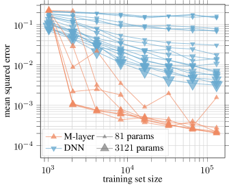
Figure 4: Learning the determinant of a $3\times 3$ matrix with M-layers and DNNs with various parameter counts and training set sizes.

Table 1: Comparison of classification performance on image recognition datasets. We compare the M-layer to three general-purpose types of architectures: fully-connected (f.c.) networks with different activation functions [LMK15], NODE [CRBD18], and ANODE [DDT19]. The sources are listed as [D] [DDT19] and [L] [LMK15].

center Architecture Convolutional? Problem Accuracy % (mean $\pm$ S.D.) Parameters Source M-LAYER no MNIST $97.99~{}\pm 0.12$ 0 0$68\,885$ NODE yes MNIST $96.40~{}\pm 0.50$ 0 0$84\,000$ [d] ANODE yes MNIST $98.20~{}\pm 0.10$ 0 0$84\,000$ [d] M-LAYER no CIFAR-10 $54.17~{}\pm 0.36$ 0 $148\,965$ SIGMOID (f.c.) no CIFAR-10 $46.63\phantom{~{}\pm 0.00}$ $8\,049\,010$ [l] ReLU (f.c.) no CIFAR-10 $56.29\phantom{~{}\pm 0.00}$ $8\,049\,010$ [l] PReLU (f.c.) no CIFAR-10 $51.94\phantom{~{}\pm 0.00}$ $8\,049\,010$ [l] Maxout (f.c.) no CIFAR-10 $52.80\phantom{~{}\pm 0.00}$ $8\,049\,010$ [l] NODE yes CIFAR-10 $53.70~{}\pm 0.20$ 0 $172\,000$ [d] ANODE yes CIFAR-10 $60.60~{}\pm 0.40$ 0 $172\,000$ [d] M-LAYER no SVHN $81.19~{}\pm 0.23$ 0 $148\,965$ NODE yes SVHN $81.00~{}\pm 0.60$ 0 $172\,000$ [d] ANODE yes SVHN $83.50~{}\pm 0.50$ 0 $172\,000$ [d]

4.4 Learning Image Datasets

We assess the performance of the M-layer on three image classification tasks: MNIST [LBBH98], CIFAR10 [Kri09], and SVHN [NWC⁺11].

The following procedure is used for all M-layer experiments in this section. The training set is randomly shuffled and $10\%$ of the shuffled data is set aside as a validation set. The M-layer dimensions are $d=35$ and $n=30$, which are chosen by a random search in the interval $[1,100]$. An SGD optimizer is used with initial learning rate of $10^{-3}$, momentum $0.9$, and batch size $32$. The learning rate is chosen as the largest value that gave a stable performance, momentum is fixed, and the batch size is chosen as the best-performing in $(32,64)$. The learning rate is reduced by $80\%$ following $5$ epochs without validation accuracy improvement. Training is carried for a maximum of $150$ epochs, with early stopping after $15$ epochs without validation accuracy improvement. The model that performs best on the validation set is tested. Accuracy values are averaged over at least $30$ runs.

We compare the performance of the M-layer with three recently-studied general-purpose architectures. As the M-layer is a novel architecture and no additional engineering is performed to obtain the results in addition to the regularization process described above, we only compare it to other generic architectures that also use no architectural modifications to improve their performance.

(a) DNN

(b) M-layer

Figure 5: Learning the $5\times 5$ determinant. Each scatter plot shows $5000$ points, each corresponding to a pair (true determinant, learnt determinant).

The results are shown in Table 1. The M-layer outperforms multiple fully-connected architectures (with sigmoid, parametric ReLU, and maxout activations), while employing significantly fewer parameters. The M-layer also outperforms the NODE network, which is based on a convolutional architecture. The networks that outperform the M-layer are the ReLU fully-connected network, which has significantly more parameters, and the ANODE network, which is an improved version of NODE and is also based on a convolutional architecture.

Computing a matrix exponential may seem computationally demanding. To investigate this, we compare the training time of an M-layer with that of a DNN with similar number of parameters. Table 2 shows that the M-layer only takes approximately twice as much time to train.

We also compute the robustness bounds of the M-layer trained on CIFAR-10, as described in Section 3.7. We train $n=20$ models with $\delta_{in}\approx 200$, $\lVert S\rVert_{2}\approx 3$, and $\lVert M\rVert_{2}$ typically a value between $3$ and $4$. The maximum $L_{2}$ variation of the vector of accumulated evidences is $\approx 1$. This results in a typical $L_{\infty}$ bound for robustness of $\approx 10^{-5}$ on the whole set of correctly classified CIFAR-10 test samples. In comparison, an analytical approach to robustness similar to ours [PRGS17], which uses a layer-by-layer analysis of a traditional DNN, achieves $L_{2}$ bounds of $\approx 10^{-9}$. Figure 6 shows the distribution of $L_{\infty}$ bounds obtained for the M-layer.

Table 2: Comparison of training time per epoch for CIFAR-10 on a Nvidia V100 GPU. The M-layer dimensions are $d=35$ and $n=30$. The DNN has $4$ layers of size $43-100-100-10$.

Architecture	Parameters	Training time
M-Layer	$148965$	$8.67s~{}\pm 0.56$
ReLU DNN	$147649$	$4.12s~{}\pm 0.26$

Early experiments show promising results on the same datasets when applying advanced machine learning techniques to the M-layer, such as combining the M-layer with convolutional layers and using dropout for regularization. As the scope of this paper is to introduce the basics of this architecture, we defer this study to future work.

5 Conclusion

This paper introduces a novel model for supervised machine learning based on a single matrix exponential, where the matrix to be exponentiated depends linearly on the input. The M-layer is a powerful yet mathematically simple architecture that has universal approximator properties and that can be used to learn and extrapolate several problems that traditional DNNs have difficulty with.

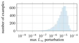
Figure 6: Maximum $L_{\infty}$ perturbation on the correctly classified CIFAR-10 test samples that is guaranteed not to produce a misclassification.

An essential property of the M-layer architecture is its natural ability to learn input feature crosses, multivariate polynomials and periodic functions. This allows it to extrapolate learning to domains outside the training data. This can also be achieved in traditional networks by using specialized units that perform custom operations, such as multiplication or trigonometric functions. However, the M-layer can achieve this with no additional engineering.

In addition to several mathematical benchmarks, we have shown that the M-layer performs competitively on standard image recognition datasets when compared to non-specialized architectures, sometimes employing substantially fewer parameters. In exchange for the benefits it provides, the M-layer only takes around twice as much time as a DNN with the same number of parameters to train, while also considerably simplifying hyperparameter search.

Finally, another desirable property of the M-layer is that it allows closed-form robustness bounds, thanks to its powerful but relatively simple mathematical structure.

We provide source code in TensorFlow that can be used to train and further explore the capabilities of the M-layer. Future work will focus on adapting the M-layer for specialized tasks, such as hybrid architectures for image recognition, and advanced regularization methods inspired by the connection between the M-layer and Lie groups.

Appendix A Appendix

A.1 Universal Approximation Theorem

We show that a single M-layer model that uses sufficiently large matrix size is able to express any polynomial in the input features. This is true even when we restrict the matrix to be exponentiated to be nilpotent or, more specifically, strictly upper triangular. So, for classification problems, M-layer architectures are a superset of multivariate polynomial classifiers, where matrix size constrains the complexity of the polynomial.

Theorem 1 (Expressibility of polynomials).

Given a polynomial $p(x_{1},\dots,x_{n})$ in $n$ variables, we can choose weight tensors for the M-layer such that it computes $p$ exactly.

Proof.

The tensor contraction applied to the result of matrix exponentiation can form arbitrary linear combinations, and is therefore able to compute any polynomial given a matrix that contains the constituent monomials up to constant factors. Thus, it suffices to prove that we can produce arbitrary monomials in the exponentiated matrix.

Given a monomial $m$ of degree $d-1$, we consider the $d\times d$ matrix $U$, that has the $d-1$ (possibly repeated) factors of the monomial on the first upper diagonal and zeros elsewhere. Let us consider powers of $U$. It can be shown that all elements of $U^{i}$ are equal to $0$, except for the $i$-th upper diagonal, and that the value in the ($d-1$)-th upper diagonal of $U^{d-1}$, which contains only one element, is the product of the entries of the first upper diagonal of $U$. This is precisely the monomial $m$ we started with. By the definition of the exponential of the matrix, $\exp(U)$ then contains $\frac{m}{(d-1)!}$, which is the monomial up a constant factor.

Given a polynomial $p$ constiting of $t$ monomials, for each $1\leq i\leq t$, we form matrices $U_{i}$ for the corresponding monomial $m_{i}$ of $p$, as described above. Then we build the diagonal block matrix $U=\operatorname{diag}(U_{1},\dots,U_{t})$. It is clear that $\exp(U)=\operatorname{diag}(\exp(U_{1}),\dots,\exp(U_{k}))$, so we can find all monomials of $p$ in $\exp(U)$. ∎

To illustrate the proof, we look at a monomial $m=abcd$.

$$\begin{array}[]{rcl}U&=&\left(\begin{array}[]{rrrrr}0&a&0&0&0\\ 0&0&b&0&0\\ 0&0&0&c&0\\ 0&0&0&0&d\\ 0&0&0&0&0\end{array}\right)\\ {}\hfil&{}\hfil&{}\\ \exp(U)&=&\left(\begin{array}[]{rrrrr}1&a&\frac{1}{2}ab&\frac{1}{6}abc&\frac{1}{24}abcd\\ 0&1&b&\frac{1}{2}bc&\frac{1}{6}bcd\\ 0&0&1&c&\frac{1}{2}cd\\ 0&0&0&1&d\\ 0&0&0&0&1\end{array}\right)\end{array}$$

The M-layers constructed here only make use of nilpotent matrices. When using this property as a constraint, the size of the M-layer can be effectively halved in the implementation.

The construction from Theorem 1 can be adapted to express not only a multivariate polynomial, i.e. a function to $\mathbb{R}^{1}$, but also functions to $\mathbb{R}^{k}$, which restrict to a polynomial in each coordinate. This, together with the Stone-Weierstrass theorem [Sto48], implies the following:

Corollary 2.

For any continuous function ${f\colon[a,b]^{n}\rightarrow\mathbb{R}^{m}}$ and any $\epsilon>0$, there exists an M-layer model that computes a function $g$ such that $|f(x_{0},\dots,x_{n-1})_{j}-g(x_{0},\dots,x_{n-1})_{j}|<\epsilon$ for all $0\leq j\leq m$.

A.1.1 Optimality of construction

While our proof is constructive, we make no claim that the size of the matrix used in the proof is optimal and cannot be decreased. Given a multivariate polynomial of degree $d$ with $t$ monomials, the size of the matrix we construct would be $t(d+1)^{2}$. In fact, by slightly adapting the construction, we can obtain a size of matrix that is $td^{2}+1$. Given that the total number of monomials in polynomials of $n$ variables up to degree $d$ is $\binom{n+d}{d}$, it seems likely possible to construct much smaller M-layers for many polynomials. Thus, one wonders what is, for a given polynomial, the minimum matrix size to represent it with an M-layer.

As an example, we look at the determinant of a $3\times 3$-Matrix. If the matrix is

$$\left(\begin{array}[]{rrr}a&b&c\\ d&e&f\\ g&h&i\end{array}\right),$$

then the determinant is the polynomial $aei-afh-bdi+bfg+cdh-ceg$. From Theorem 1, we know that it is possible to express this polynomial perfectly with a single M-layer. However, already an M-layer of size $8$ is sufficient to represent the determinant of a $3\times 3$ matrix: If

$$M=\left(\begin{array}[]{rrrrrrrr}0&0&i&f&0&0&0&0\\ 0&0&h&e&0&0&0&0\\ 0&0&0&0&2d&-2f&0&0\\ 0&0&0&0&-2g&2i&0&0\\ 0&0&0&0&0&0&3c&-3b\\ 0&0&0&0&0&0&3a&0\\ 0&0&0&0&0&0&0&0\\ 0&0&0&0&0&0&0&0\end{array}\right)$$ (4)

then $\exp(M)$ is

$$\left(\begin{smallmatrix}1&0&i&f&-fg+di&0&-cfg+cdi&bfg-bdi\\ 0&1&h&e&-eg+dh&-fh+ei&-ceg+aei+cdh-afh&beg-bdh\\ 0&0&1&0&2d&-2f&3cd-3af&-3bd\\ 0&0&0&1&-2g&2i&-3cg+3ai&3bg\\ 0&0&0&0&1&0&3c&-3b\\ 0&0&0&0&0&1&3a&0\\ 0&0&0&0&0&0&1&0\\ 0&0&0&0&0&0&0&1\end{smallmatrix}\right),$$

the sum of $\exp(M)_{0,7}$ and $\exp(M)_{1,6}$ is exactly this determinant. The permanent of a $3\times 3$ matrix can be computed with an almost identical matrix, by removing all minus signs.

References

- [CRBD18] Tian Qi Chen, Yulia Rubanova, Jesse Bettencourt, and David K Duvenaud. Neural Ordinary Differential Equations. In S Bengio, H Wallach, H Larochelle, K Grauman, N Cesa-Bianchi, and R Garnett, editors, Advances in Neural Information Processing Systems 31, pages 6571–6583. Curran Associates, Inc., 2018. NeurIPS.
- [DDT19] Emilien Dupont, Arnaud Doucet, and Yee Whye Teh. Augmented neural odes. In H. Wallach, H. Larochelle, A. Beygelzimer, F. d’Alché Buc, E. Fox, and R. Garnett, editors, Advances in Neural Information Processing Systems 32, pages 3134–3144. Curran Associates, Inc., 2019.
- [GB10] Xavier Glorot and Yoshua Bengio. Understanding the difficulty of training deep feedforward neural networks. In Proceedings of the thirteenth international conference on artificial intelligence and statistics, pages 249–256, 2010.
- [Gil08] Robert Gilmore. Lie groups, physics, and geometry: an introduction for physicists, engineers and chemists. Cambridge University Press, 2008.
- [Gil12] Robert Gilmore. Lie groups, Lie algebras, and some of their applications. Courier Corporation, 2012.
- [GWFM+13] Ian J. Goodfellow, David Warde-Farley, Mehdi Mirza, Aaron Courville, and Yoshua Bengio. Maxout networks. In 30th International Conference on Machine Learning, ICML 2013, number PART 3, pages 2356–2364, 2013.
- [Hig05] Nicholas J. Higham. The Scaling and Squaring Method for the Matrix Exponential Revisited. SIAM Journal on Matrix Analysis and Applications, 26(4):1179–1193, 2005.
- [Kri09] Alex Krizhevsky. Learning Multiple Layers of Features from Tiny Images. Technical report, 2009.
- [LBBH98] Y. Lecun, L. Bottou, Y. Bengio, and P. Haffner. Gradient-based learning applied to document recognition. Proceedings of the IEEE, 86(11):2278–2324, 1998.
- [LMK15] Zhouhan Lin, Roland Memisevic, and Kishore Konda. How far can we go without convolution: Improving fully-connected networks. pages 1–10, 2015.
- [MV03] Cleve Moler and Charles Van Loan. Nineteen Dubious Ways to Compute the Exponential of a Matrix, Twenty-Five Years Later. SIAM Review, 45(1):3–49, 2003.
- [NWC+11] Yuval Netzer, Tao Wang, Adam Coates, Alessandro Bissacco, Bo Wu, and Andrew Y Ng. Reading Digits in Natural Images with Unsupervised Feature Learning. In NIPS Workshop on Deep Learning and Unsupervised Feature Learning 2011, 2011.
- [PRGS17] Jonathan Peck, Joris Roels, Bart Goossens, and Yvan Saeys. Lower bounds on the robustness to adversarial perturbations. In Advances in Neural Information Processing Systems, pages 804–813, 2017.
- [PS91] J. Park and I. W. Sandberg. Universal Approximation Using Radial-Basis-Function Networks. Neural Computation, 3(2):246–257, 1991.
- [RC94] Horn Roger and R Johnson Charles. Topics in matrix analysis. Cambridge University Press, 1994.
- [RHM86] D. E. Rumelhart, G. E. Hinton, and James L Mcclelland. A general framework for parallel distributed processing. In Parallel distributed processing: explorations in the microstructure of cognition, chapter 2. 1986.
- [SFH17] Sara Sabour, Nicholas Frosst, and Geoffrey E Hinton. Dynamic Routing Between Capsules. Advances in Neural Information Processing Systems 30, pages 3856–3866, 2017.
- [SGPV18] Gagandeep Singh, Timon Gehr, Markus Püschel, and Martin Vechev. Boosting robustness certification of neural networks. 2018.
- [SGPV19] Gagandeep Singh, Timon Gehr, Markus Püschel, and Martin Vechev. An abstract domain for certifying neural networks. Proceedings of the ACM on Programming Languages, 3(POPL):1–30, 2019.
- [Sto48] Marshall H Stone. The generalized Weierstrass approximation theorem. Mathematics Magazine, 21(5):237–254, 1948.
- [THR+18] Andrew Trask, Felix Hill, Scott Reed, Jack Rae, Chris Dyer, and Phil Blunsom. Neural Arithmetic Logic Units. Advances in Neural Information Processing Systems, 2018-Decem:8035–8044, 2018.