Abstract

We derive a QCD sum rule for the inverse moment of the $B_{s}$-meson light-cone distribution amplitude in HQET. Within this method, the $SU(3)_{fl}$ symmetry violation is traced to the strange quark mass and to the difference between strange and nonstrange quark condensate densities. We predict the ratio of inverse moments $\lambda_{B_{s}}/\lambda_{B}=1.19\pm 0.14$ which can be used in various applications of these distribution amplitudes to the analyses of $B_{s}$-meson decays, provided an accurate value of $\lambda_{B}$ is available from other sources, such as the $B\to\ell\nu_{\ell}\gamma$ decay.

1 Introduction

Heavy mesons carrying bottom and strange quantum numbers have attracted increasing attention due to the large data sample which has been collected by the LHCb collaboration over the last years. With the new precise measurements it becomes increasingly important to also get more accurate theoretical predictions. This involves, in particular, reliable estimates of the $SU(3)$ flavour symmetry violation, to be taken into account while analyzing the $B_{s}$ data and comparing to the results for nonstrange bottom mesons. Among important quantities in the theoretical analyses are the light-cone distribution amplitudes (DAs) of heavy mesons. While these quantities were extensively studied for nonstrange bottom mesons, the $SU(3)_{fl}$ violating effects for $B_{s}$ have not yet been estimated.

The light-cone DAs of $B$-meson introduced [1] in the framework of Heavy Quark Effective Theory (HQET) (see also [2]) describe momentum distribution of the light quark in a heavy pseudoscalar meson. These DAs enter various factorization formulas for the exclusive decays of $B$-meson (see e.g. [3, 4, 5, 6, 7]). They also provide the main nonperturbative input in one of the versions [8] of QCD light-cone sum rules for $B$-meson form factors. In all these applications, the key parameter is the inverse moment of the leading (lowest twist) $B$-meson DA.

Evidently, the mass of the light $u,d$ quarks plays no role in the $B_{u,d}$ meson DAs. It can safely be neglected not only in comparison with any of the large scales involved in an exclusive $B_{u,d}$ decay, but also with respect to typical hadronic scales of $\mathcal{O}(\Lambda_{QCD})$. This is, however, not the case for the $s$-quark. In fact, the leptonic decay constants of bottom mesons exhibit an appreciable $SU(3)_{fl}$ symmetry violation. The ratio $f_{B_{s}}/f_{B_{u,d}}$ calculated from the lattice QCD deviates by about $20\%$ from the unity [9]. QCD sum rules (see e.g. [10, 11]) predict this ratio in the same ballpark. Nevertheless, the influence of the strange quark mass on the inverse moment of $B_{s}$-meson DA has never been investigated. One of the reasons is that the heavy meson DAs are not yet accessible in lattice QCD (for the first exploratory studies see e.g. [12, 13]). For simplicity, the inverse moments of all bottom mesons are assumed equal, as for example in the QCD factorization analysis of nonleptonic $B$ and $B_{s}$ decays [14].

The $B_{s}$-meson DA is needed to describe many important decay channels, such as the $\bar{B}_{s}\to K^{(*)},\phi$ semileptonic and Flavor Changing Neutral Current (FCNC) transitions, as well as various nonleptonic $B_{s}$ decays, where precision predictions for observables are vitally needed. It is therefore timely to make a quantitative assessment of the $SU(3)_{fl}$ symmetry violation in the bottom meson DAs.

In the future, accurate measurements of the photoleptonic decay $B^{-}\to\ell^{-}\bar{\nu}_{\ell}\gamma$ will allow to constrain the inverse moment of the $B$-meson DA using a well elaborated factorization formula for the form factors of this decay (the most recent analyses can be found in [15, 16, 17]). There is no such channel available for the $B_{s}$-meson DA. For example, the FCNC decay $B_{s}\to\ell^{+}\ell^{-}\gamma$ is “contaminated” by nonlocal hadronic effects which are not simply reducible to DAs. In this situation, a theory estimate of the $SU(3)_{fl}$ violation in the inverse moment is definitely useful.

In this paper, we obtain the inverse moments of the $B_{s}$ meson from the QCD sum rule in HQET. We closely follow the method used in [1, 19] for the $B$ - meson DA, but, in contrast, we do not attempt to determine the shape of DA. Instead, we obtain a QCD sum rule directly for the inverse moment. Including the $\mathcal{O}(m_{s})$ effects in the perturbative part and taking into account the difference between strange and nonstrange quark condensates, we estimate the inverse moment of $B_{s}$-meson DA and, as a byproduct, the inverse moment of the $B$-meson DA. Finally, we predict the ratio of the two inverse moments with a lesser uncertainty.

In what follows, in Section 2 we specify the method combining the two QCD sum rules in HQET: the one for the leptonic decay constant and the another one for the DA. The effects of strange quark mass are calculated and taken into account. Our numerical results are presented in Section 3 and we summarize in Section 4. The Appendix contains some useful details of the calculation.

2 The method

2.1 Sum rule for the $B_{s}$ decay constant

To explain how the $SU(3)_{fl}$ violating difference between strange and nonstrange bottom mesons emerges, it is instructive to begin with the sum rule for the leptonic decay constant. We consider it first in QCD with finite masses of $b$ and $s$ quarks, and then take the limit of infinitely heavy $b$-quark, performing a transition to the HQET sum rule. We also need the latter sum rule to fix the input parameters for the sum rule determination of the $B_{s}$-meson DAs.

We start with the correlation function of the two pseudoscalar heavy-light currents defined in the standard way:

$$\Pi_{5q}(q^{2})=i\!\int\!d^{4}x\,e^{iq\cdot x}\langle 0|T\{j_{5q}(x)j_{5q}^{\dagger}(0)\}|0\rangle\,,$$ (1)

where $j_{5q}$ is the divergence of the axial current $j_{5q}=(m_{b}+m_{q})\bar{q}i\gamma_{5}b$ with $m_{b}$ and $m_{q}$ being the $b$-quark and light-quark ($q=u,d,s$) mass, respectively. In what follows, we neglect the $u,d$-quark masses, assuming isospin and chiral symmetry. We also adopt the $\overline{MS}$ scheme for the $s$- and $b$-quark masses. The decay constant of the pseudoscalar $B\equiv B_{u,d}$- and $B_{s}$-meson is defined, respectively, as

$$\langle 0|j_{5u(d)}|B(p_{B})\rangle=m_{B}^{2}f_{B}\,,~{}~{}\langle 0|j_{5s}|B_{s}(p_{B_{s}})\rangle=m_{B_{s}}^{2}f_{B_{s}}\,.$$ (2)

The correlation function (1) satisfies a double-subtracted dispersion relation which, after the Borel transformation $|q^{2}|\to M^{2}$, takes the form

$$\Pi_{5q}(M^{2})=\frac{1}{\pi}\int\limits_{0}^{\infty}\!ds\,e^{-s/M^{2}}\mbox{Im}\Pi_{5q}(s)\,,$$ (3)

in which subtraction terms vanish. To obtain the sum rule, we use the operator product expansion (OPE) of the correlation function $\Pi_{5q}$ valid at deep spacelike $q^{2}\ll m_{b}^{2}$ or, equivalently, at sufficiently large $M^{2}$. The result $\Pi_{5q}^{\rm(OPE)}(M^{2})$ consists of the perturbative and nonperturbative (vacuum condensate) parts:

$$\Pi^{\rm(OPE)}_{5q}(M^{2})=\int\limits_{(m_{b}+m_{s})^{2}}^{\infty}\!ds\,e^{-s/M^{2}}\rho^{\rm(pert)}_{5q}(s)+\Pi^{\rm(cond)}_{5q}(M^{2})\,,$$ (4)

where the perturbative contribution is written in a dispersion integral form with the spectral density

$$\rho^{\rm(pert)}_{5q}(s)=\frac{1}{\pi}\text{Im}\,\Pi^{\rm(pert)}_{5q}(s)\,.$$

Adopting the usual quark-hadron duality ansatz, the hadronic spectral density in Eq. (3) is approximated by the contribution of the lowest pseudoscalar bottom meson and the OPE perturbative density taken above an effective threshold. Considering, for definiteness, the $B_{s}$ case of our interest, we have:

$$\frac{1}{\pi}\mbox{Im}\Pi_{5s}(s)=m_{B_{s}}^{4}f_{B_{s}}^{2}\delta(s-m_{B_{s}}^{2})+\theta(s-s_{0s})\rho^{\rm(pert)}_{5s}(s)\,.$$ (5)

Substituting the above expression in r.h.s. of Eq. (3) and using for the l.h.s. the OPE result (4), we arrive at the sum rule:

$$m_{B_{s}}^{4}f_{B_{s}}^{2}e^{-m_{B_{s}}^{2}/M^{2}}=\!\!\!\!\int\limits_{(m_{b}+m_{s})^{2}}^{s_{0s}}\!\!\!ds\,\rho_{5s}^{\rm(pert)}(s)e^{-s/M^{2}}+\Pi^{\rm(cond)}_{5q}(M^{2})\,.$$ (6)

The leading-order (LO) perturbative term in the OPE of the spectral density arises from the simple quark-antiquark loop diagram and is given by

$$\rho^{\rm(pert,LO)}_{5s}(s)=\frac{3}{8\pi^{2}}(m_{b}+m_{s})^{2}\left(1-\frac{(m_{b}-m_{s})^{2}}{s}\right)\lambda^{1/2}(s,m_{b}^{2},m_{s}^{2})\,,$$ (7)

where $\lambda(x,y,z)\equiv x^{2}+y^{2}+z^{2}-2xy-2xz-2yz$ is the Källén function. Note that here it is more convenient to use the above spectral density than to expand it in the powers of $m_{s}$ as it is customary in the literature (see e.g., [10, 11]). To complete the sum rule, the gluon radiative corrections will be added to the r.h.s. of Eq. (6). All necessary expressions can be found e.g., in [11] .

As a next step, we transform the variables and parameters in the sum rule (6) in order to separate the heavy $b$-quark scale and pave the way to the sum rule in HQET. In our case, there is a nonvanishing $s$-quark mass involved in this transformation. We express the external momentum squared in the correlation function (1) in terms of a new variable $\omega$:

$$q^{2}=m_{b}^{2}+2m_{b}\,\omega\,,$$ (8)

and, simultaneously, replace the $B_{s}$-meson mass by

$$m_{B_{s}}=m_{b}+\bar{\Lambda}_{s}\,,$$ (9)

so that $\omega$ and $\bar{\Lambda}_{s}$ do not scale with the $b$-quark mass.

The relation (8) yields for the variable $q^{2}=s$ in the timelike region:

$$s=m_{b}^{2}+2m_{b}\omega^{\prime}\,,$$ (10)

so that $\omega^{\prime}$ will serve as the integration variable in the sum rule. According to Eq. (9), the position of the $B_{s}$ pole at $s=m_{B_{s}}^{2}$ corresponds to $\omega^{\prime}=\bar{\Lambda}_{s}$ and the quark-antiquark threshold of the loop diagram at $s=(m_{b}+m_{s})^{2}$ turns into $\omega^{\prime}=m_{s}$. Note that all these relations are valid up to $O(1/m_{b})$ corrections which vanish in the $m_{b}\to\infty$ limit. Furthermore, in accordance with the above definitions, we transform the threshold and the Borel parameter, respectively:

$$s_{0s}=m_{b}^{2}+2m_{b}\,\omega_{0s},~{}~{}~{}\mbox{and}~{}~{}~{}M^{2}=2m_{b}\tau\,,$$ (11)

where the parameter $\omega_{0s}$ and the variable $\tau$ again do not scale with the $b$-quark mass. Note, on the other hand, that the $B_{s}$ binding energy $\bar{\Lambda}_{s}$ and the effective threshold $\omega_{0s}$ both implicitly depend on $m_{s}$. Applying Eqs. (8)–(11) to Eq. (6), we then take the limit $m_{b}\to\infty$, transforming this sum rule to its HQET form:

$$\big{[}F_{B_{s}}(\mu)\big{]}^{2}e^{-\bar{\Lambda}_{s}/\tau} = \frac{3}{\pi^{2}}\int\limits_{m_{s}}^{\omega_{0s}}\!d\omega^{\prime}\,e^{-\omega^{\prime}/\tau}(\omega^{\prime}+m_{s})\sqrt{\omega^{\prime 2}-m_{s}^{2}}$$ (12)

$$+ \frac{3\alpha_{s}}{\pi^{3}}\int\limits_{0}^{\omega_{0s}}\!d\omega^{\prime}\,e^{-\omega^{\prime}/\tau}\omega^{\prime 2}\,\left(\frac{17}{3}+\frac{4\pi^{2}}{9}-2\ln\frac{2\omega^{\prime}}{\mu}\right)$$

$$- \langle\bar{s}s\rangle\left[1+\frac{2\alpha_{s}}{\pi}-\frac{m_{0}^{2}}{16\tau^{2}}\right]\,,$$

where $F_{B_{s}}$ is the decay constant in HQET, related at the $\mathcal{O}(\alpha_{s})$ accuracy to the one defined in Eq. (2):

$$f_{B_{s}}\sqrt{m_{B_{s}}}=F_{B_{s}}(\mu)\left[1+\frac{C_{F}\alpha_{s}}{4\pi}\left(3\ln\frac{m_{b}}{\mu}-2\right)+\ldots\right],$$ (13)

and $\mu$ is the renormalization scale. The expression for the perturbative LO part coincides with the one in [18] where the light-quark mass was retained in the heavy-quark limit of the correlation function (1). Furthermore, in the second line of Eq. (12) we have added the $\mathcal{O}(\alpha_{s})$ gluon radiative corrections in HQET taking them from [19] . In the third line we include the condensate contributions, where $\langle\bar{s}s\rangle$ denotes the strange quark condensate density and $m_{0}^{2}$ is the ratio of the quark-gluon and quark condensates. Note that in the sum rule (12), we have neglected the very small effects of $\mathcal{O}(\alpha_{s}m_{s})$ in the perturbative spectral density (hence, the zero limit in the second integral in Eq. (12)) as well as in the quark condensate term. In addition, we assume that the ratio $m_{0}^{2}$ is the same for all three light quarks and neglect the numerically insignificant contributions of gluon and four-quark condensates.

The sum rule (12) can also be derived in the framework of HQET as it was done for the nonstrange $B$-meson in [22, 20, 21]. One starts from the correlation function of currents containing the effective heavy quark field $h_{v}$, so that the external four-momentum is $k=q-m_{b}v$. In this case, the effective variable $\omega=k\cdot v$, where $v=(1,\vec{0})$ is the velocity four-vector, replaces $q^{2}$, and the deep spacelike region $q^{2}\ll m_{b}^{2}$ corresponds to the external off-shell energy $\omega\ll 0$. Accordingly, the dispersion relation in the variable $\omega$ is used with the $B_{s}$ pole located at $\omega=\bar{\Lambda}_{s}$ and the duality interval $m_{s}<\omega<\omega_{0s}$. The HQET state of a $B_{(s)}$-meson differs from the state in Eq. (2) by a normalization factor:

$$|B_{(s)}(v)\rangle=\big{(}m_{B_{(s)}}\big{)}^{-1/2}|B_{(s)}(p_{B_{s}})\rangle\,.$$ (14)

The HQET sum rule for the nonstrange $B$-meson decay constant in the adopted approximation is simply obtained from Eq. (12) putting $m_{s}\to 0$ and replacing

$$\bar{\Lambda}_{s}\to\bar{\Lambda},~{}~{}\omega_{0s}\to\omega_{0}\,,~{}~{}~{}\langle\bar{s}s\rangle\to\langle\bar{u}u\rangle\simeq\langle\bar{d}d\rangle\,.$$ (15)

The definitions (8) and (10) are the same, but the lower limit of the integration over $\omega^{\prime}$ shifts from $m_{s}$ to zero. A comparison of the sum rules for $F_{B_{s}}$ and $F_{B}$ reveals several contributions to the $SU(3)_{fl}$ violation. One of them is due to the $m_{s}$-dependence of the perturbative spectral density in (12). Note that this effect is of $\mathcal{O}(m_{s}/\omega_{0})\sim\mathcal{O}(m_{s}/\tau)$, that is, parametrically enhanced with respect to the terms proportional to $m_{s}/m_{b}$ which have vanished in the infinitely heavy quark limit. An additional $SU(3)_{fl}$ violation effect in the OPE of the correlation function revealed on r.h.s. of Eq. (12) is caused by the difference between the strange and nonstrange quark condensate densities. This nonperturbative effect intrinsically depends on the $s$-quark mass, however this dependence cannot be represented in an explicit form. In the sum rule, the $s$-quark mass effects in the OPE are balanced in the hadronic part by the differences between the effective thresholds ($\omega_{0s}$ versus $\omega_{0}$) and the binding energies. For the latter we have the relation:

$$\bar{\Lambda}_{s}=\bar{\Lambda}+m_{B_{s}}-m_{B}\,.$$ (16)

In the numerical analysis below, we will use the sum rule (12) and its counterpart for $B$-meson to estimate the value of the continuum thresholds $\omega_{0}$ and $\omega_{0s}$. To this end, each sum rule is differentiated with respect to $-1/\tau$ and then divided by itself. In the resulting relations, the dependence on the decay constants $F_{B}$ and $F_{B_{s}}$ drops out, allowing us to fix $\omega_{0}$ and $\omega_{0s}$ at a certain adopted value of $\bar{\Lambda}$, whereas $\bar{\Lambda}_{s}$ is given by the relation (16).

Having revealed the scale of $SU(3)_{fl}$ symmetry violation in the decay constants of heavy-light mesons, we anticipate the effects to be in the same ballpark in more involved hadronic matrix elements, such as the DAs of $B_{s}$-meson.

2.2 Sum rule for the inverse moment of $B_{s}$ DA

The $B_{s}$-meson light-cone DA is defined as the hadronic matrix element of the bilocal operator built of an effective heavy-quark field $h_{v}$ with velocity $v$ and a strange antiquark field $\bar{s}$ located at a lightlike separation:

$$\langle 0|\bar{s}(tn)i\gamma_{5}\!\not\!n[tn,0]h_{v}(0)|\bar{B}_{s}(v)\rangle=F_{B_{s}}(\mu)\!\!\int\limits_{0}^{\infty}\!dk\,e^{-ikt}\phi^{B_{s}}_{+}(k,\mu)\,,$$ (17)

with the lightlike gauge link

$${}[tn,0]\equiv{\rm P\,exp}\left[ig\int\limits_{0}^{1}\!du\,n_{\mu}A^{\mu}(utn)\right].$$ (18)

Here $n_{\mu}$ is the lightlike vector, $n^{2}=0$, such that $n\cdot v=1$, and $t$ is an arbitrary real valued parameter. In Eq. (17) we used the general definition [1, 3] of the two-particle heavy-meson DA (see e.g. eq. (17) in [8]) and projected it onto the leading, twist-2 DA component $\phi^{B_{s}}_{+}(\omega)$, multiplying both sides of this definition by $(i\gamma_{5}\!\!\not\!n)$ and taking the trace. Note that $|\bar{B}_{s}(v)\rangle$ is the HQET state defined in Eq. (14). The variable $k$ in (17) can be interpreted as the light-cone projection of the light $s$-quark momentum. Due to non-vanishing $m_{s}$, it is natural to expect that for $B_{s}$ this variable is limited from below by $k=m_{s}$, hence in a realistic model, $\phi^{B_{s}}_{+}(k,\mu)\sim\theta(k-m_{s})$. However, here we will not dwell on reproducing the shape of the $B_{s}$-meson DA. Instead, we concentrate on our main task, that is, to obtain a sum rule estimate for the inverse moment defined as:

$$\lambda_{B_{(s)}}^{-1}(\mu)=\int\limits_{0}^{\infty}\frac{dk}{k}\,\phi^{B_{(s)}}_{+}(k,\mu)\,.$$ (19)

To achieve the goal, we largely follow the method used for the $B$-meson in [1] and upgraded in [19] to include the gluon radiative corrections (see also the review [23]). At the same time, we modify this method and obtain the sum rule directly for the inverse moment (19).

To this end, we introduce the following correlation function in HQET:

$${\cal P}_{s}(\omega,t)=i\!\int\!d^{4}xe^{-i\omega\,v\cdot x}\langle 0|T\big{\{}\bar{s}(tn)i\gamma_{5}\!\not\!n[tn,0]h_{v}(0)\bar{h}_{v}(x)i\gamma_{5}s(x)\big{\}}|0\rangle\,.$$ (20)

It contains a product of the bilocal operator (17) with the local pseudoscalar current interpolating the $B_{s}(v)$ state. The variable $\omega$ is analogous to the one introduced in Eq. (8) for a transition to HQET of a simpler two-point correlation function (1). In other words, if, instead of Eq. (20), we consider a correlation function with the finite mass $b$-quark fields and the external four-momentum $q$, then, after reparameterizing to the effective fields $h_{v}$, the four-momentum in the exponent becomes $(q-m_{b}v)=\omega v$.

The hadronic dispersion relation for the correlation function (20) follows from analyticity with respect to the effective variable $\omega$:

$${\cal P}_{s}(\omega,t)=\frac{1}{\pi}\int\limits_{0}^{\infty}d\omega^{\prime}\frac{\mbox{Im}{\cal P}_{s}(\omega,t)}{\omega^{\prime}-\omega}$$

$$=\frac{\langle 0|\bar{s}(tn)i\gamma_{5}\not\!n[tn,0]h_{v}(0)|\bar{B}_{s}(v)\rangle\langle\bar{B}_{s}(v)|\bar{h}_{v}i\gamma_{5}s|0\rangle}{2(\bar{\Lambda}_{s}-\omega)}+\dots$$

$$=\frac{\big{[}\,F_{B_{s}}(\mu)]^{2}}{2(\bar{\Lambda}_{s}-\omega)}\int\limits_{0}^{\infty}\!dk\,e^{-ikt}\phi^{B_{s}}_{+}(k,\mu)+\dots\,,$$ (21)

In the above, the contribution of the $B_{s}$ pole located at $\omega=\bar{\Lambda}_{s}$ is singled out, and we use the definition (17) together with the one for the $B_{s}$ decay constant in HQET:

$$\langle\bar{B}_{s}(v)|\bar{h}_{v}i\gamma_{5}s|0\rangle=F_{B_{s}}\,.$$ (22)

As it is usually done in QCD sum rules, the contributions of excited and continuum states with the $B_{s}$ quantum numbers, indicated in Eq. (2.2) by the ellipsis, will be approximated assuming the quark-hadron duality. Furthermore, to decrease the sensitivity to this approximation, we employ the Borel transformation in the variable $\omega$ defined in HQET as:

$${\cal B}_{\tau}f(\omega)=\lim\limits_{\{-\omega,n\}\to\infty,-\omega/n=\tau}\frac{(-\omega)^{n+1}}{n!}\left(\frac{d}{d\omega}\right)^{n}f(\omega)\equiv f(\tau)\,.$$ (23)

Applying it to Eq. (2.2), we have:

$${\cal P}_{s}(\tau,t)=\frac{1}{2}\big{[}F_{B_{s}}(\mu)]^{2}e^{-\bar{\Lambda}_{s}/\tau}\int\limits_{0}^{\infty}\!dk\,e^{-ikt}\phi^{B_{s}}_{+}(k,\mu)+\dots\,.$$ (24)

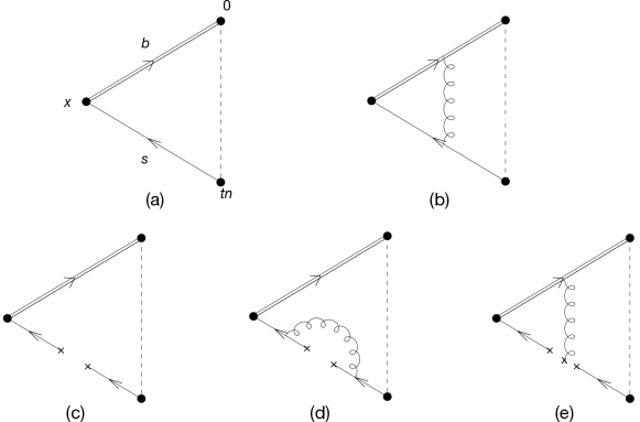
Figure 1: The diagrams contributing to the correlation function (20): (a) LO loop; (b) one of the gluon radiative corrections; (c) quark condensate contribution in LO; (d) one of the gluon radiative corrections to quark condensate; (e) quark-gluon condensate contributions. The double line describes the heavy ($b$-quark) effective field, the point at $x$ corresponds to the pseudoscalar interpolating current, the dashed interval connecting the points $0$ and $tn$ on the light-cone indicates the bilocal operator interpolating the meson DA. All possible diagrams at $\mathcal{O}(\alpha_{s})$ can be found in [19].

The next task is to obtain the OPE of the correlation function:

$${\cal P}^{\rm OPE}_{s}(\omega,t)={\cal P}^{\rm(pert)}_{s}(\omega,t)+{\cal P}^{\rm(cond)}_{s}(\omega,t)\,,$$ (25)

valid in the region $|\omega|\gg\Lambda_{QCD}$. The LO perturbative part is described by the diagram in Fig. 1(a) with a nonzero $s$-quark mass. This diagram is a simple loop, where the external momentum transfer takes place through the virtual quark and antiquark lines. The $\mathcal{O}(\alpha_{s})$ radiative gluon corrections in ${\cal P}^{\rm(pert)}_{s}$ are exemplified by one of the diagrams shown in Fig. 1(b). For these corrections we neglect the $\mathcal{O}(\alpha_{s}m_{s})$ effects, and use the formulas derived in [19]. The quark condensate contribution to ${\cal P}^{\rm(cond)}_{s}$ in LO corresponds to the diagram in Fig. 1 (c) and one of the radiative gluon corrections to this term of OPE is shown in Fig. 1 (d). In addition, both diagrams in Figs 1 (c,e) contribute to the quark-gluon condensate term. Similar to the sum rule (12), the $SU(3)_{fl}$ violation reveals itself by the $m_{s}\neq 0$ and $\langle\bar{s}s\rangle\neq\langle\bar{u}u\rangle$ effects, respectively, in the perturbative and condensate parts of the OPE (25).

The perturbative part is represented in a form of a dispersion integral in the variable $\omega^{\prime}$:

$${\cal P}^{\rm(pert)}_{s}(\omega,t)=\frac{1}{\pi}\int\limits_{m_{s}}^{\infty}\!d\omega^{\prime}\,\frac{\mbox{Im}\,{\cal P}^{\rm(pert)}_{s}(\omega,t)}{\omega^{\prime}-\omega}\,.$$ (26)

Note that the lower limit of the integration is equal to the threshold of the quark loop with $m_{s}\neq 0$ in HQET (cf. the LO term in Eq. (12)). Using the relation (26) in Eq. (25) and performing Borel transformation, we equate the result to Eq. (24):

$$\frac{1}{2}\big{[}F_{B_{s}}(\mu)]^{2}e^{-\bar{\Lambda}_{s}/\tau}\int\limits_{0}^{\infty}\!dk\,e^{-ikt}\phi^{B_{s}}_{+}(k,\mu)+\dots=\frac{1}{\pi}\int\limits_{m_{s}}^{\infty}\!d\omega^{\prime}\,e^{-\omega^{\prime}/\tau}\,\mbox{Im}{\cal P}^{\rm(pert)}_{s}(\omega^{\prime},t)+{\cal P}^{\rm(cond)}_{s}(\tau,t)\,.$$ (27)

Applying the quark-hadron duality approximation, we equate the sum of contributions on l.h.s. located above the $B_{s}$ pole to the part of the integral on r.h.s. above the threshold $\omega_{0s}$ which is taken the same as in the sum rule (12). We finally obtain:

$$\frac{1}{2}\big{[}F_{B_{s}}(\mu)]^{2}e^{-\bar{\Lambda}_{s}/\tau}\int\limits_{0}^{\infty}\!dk\,e^{-ikt}\phi^{B_{s}}_{+}(k,\mu)=\frac{1}{\pi}\int\limits_{m_{s}}^{\omega_{0s}}\!d\omega^{\prime}\,e^{-\omega^{\prime}/\tau}\,\mbox{Im}{\cal P}^{\rm(pert)}_{s}(\omega^{\prime},t)+{\cal P}^{\rm(cond)}_{s}(\tau,t)\,.$$ (28)

Calculating the perturbative spectral density and condensate term from the diagrams in Fig. 1, it is possible to reduce both of them to the half-Fourier transforms similar to the l.h.s.:

$$\mbox{Im}{\cal P}^{\rm(pert)}_{s}(\omega^{\prime},t)=\int\limits_{0}^{\infty}\!dk\,e^{-ikt}\,\mbox{Im}\widetilde{{\cal P}}^{\rm(pert)}_{s}(\omega^{\prime},k)\,,~{}~{}{\cal P}^{\rm(cond)}_{s}(\tau,t)=\int\limits_{0}^{\infty}\!dk\,e^{-ikt}\,\widetilde{{\cal P}}^{\rm(cond)}_{s}(\tau,k)\,.$$ (29)

The calculation details are presented in Appendix. For the NLO $\mathcal{O}(\alpha_{s})$ corrections, we neglect the $\mathcal{O}(m_{s})$ effects and employ the results of [19] obtained for the correlation function with a massless quark. The condensate contributions in the form (29) are also inferred from the results of [19] replacing $\langle\bar{u}u\rangle\to\langle\bar{s}s\rangle$.

Substituting Eq. (29) in Eq. (28) and comparing the integrands on both sides, we are in a position to read off the $B_{s}$-meson DA as a function of the variable $k$, in the same way as it has been done for the $B$-meson DA in [1, 19] (see also [8] where analogous sum rules have been obtained for the $B$-meson quark-antiquark-gluon DAs ). However, as noted already in [1, 19] and discussed in detail below, the sum rule based on a local OPE yields a DA which is not a smooth function, since the local condensate contributions produce terms of the form $\phi_{+}(k)\sim\delta(k)$. The region of small $k$ has to be regularized by introducing a nonlocality into the condensate contribution. In addition, we expect also modifications of the $B_{s}$ DA at small $k$, due to the threshold effects from $m_{s}\neq 0$.

In this work, we are eventually interested in the inverse moment (19). Hence, we will avoid the determination of the DA shape, noticing that we can directly obtain a sum rule for the inverse moment, integrating both sides of (28) over the parameter $t$ for $0\leq t\leq\infty$ :

$$\frac{1}{2}\big{[}\lambda_{B_{s}}(\mu)\big{]}^{-1}\big{[}F_{B_{s}}(\mu)]^{2}e^{-\bar{\Lambda}_{s}/\tau}=\frac{1}{\pi}\int\limits_{m_{s}}^{\omega_{0s}}\!d\omega^{\prime}\,e^{-\omega^{\prime}/\tau}\int\limits_{0}^{\infty}\!\frac{dk}{k}\,\mbox{Im}\widetilde{{\cal P}}^{\rm(pert)}_{s}(\omega^{\prime},k)+\int\limits_{0}^{\infty}\!\frac{dk}{k}\,\widetilde{{\cal P}}^{\rm(cond)}_{s}(\tau,k)\,.$$ (30)

The perturbative part of this sum rule consists of the LO and NLO parts:

$$\mbox{Im}\widetilde{{\cal P}}^{\rm(pert)}_{s}(\omega^{\prime},k)=\mbox{Im}\widetilde{{\cal P}}^{\rm(pert,LO)}_{s}(\omega^{\prime},k)+\mbox{Im}\widetilde{{\cal P}}^{\rm(pert,NLO)}_{s}(\omega^{\prime},k)\,.$$

The LO part, at $m_{s}\neq 0$, derived in the Appendix reads:

$$\mbox{Im}\widetilde{{\cal P}}^{\rm(pert,LO)}_{s}(\omega^{\prime},k)=\frac{3}{4\pi}\theta\big{(}k_{\rm max}(\omega^{\prime})-k\big{)}\theta\big{(}k-k_{\rm min}(\omega^{\prime})\big{)}(k+m_{s})\,,$$ (31)

where

$$k_{\rm max,\,min}(\omega^{\prime})=\omega^{\prime}\pm\sqrt{\omega^{{}^{\prime}2}-m_{s}^{2}}\,.$$ (32)

The NLO part (at $m_{s}=0$) is taken from [19]; we only change the order of integrations. Performing the $k$-integration of the LO part (31), we obtain a more detailed expression for the sum rule (30):

$$\big{[}\lambda_{B_{s}}(\mu)\big{]}^{-1}\big{[}F_{B_{s}}(\mu)]^{2}e^{-\bar{\Lambda}_{s}/\tau}=\frac{3}{2\pi^{2}}\int\limits_{m_{s}}^{\omega_{0s}}\!d\omega^{\prime}\,e^{-\omega^{\prime}/\tau}\Bigg{[}2\sqrt{\omega^{{}^{\prime}2}-m_{s}^{2}}+m_{s}\log\frac{\omega^{\prime}+\sqrt{\omega^{{}^{\prime}2}-m_{s}^{2}}}{\omega^{\prime}-\sqrt{\omega^{{}^{\prime}2}-m_{s}^{2}}}\Bigg{]}$$

$$+\frac{\alpha_{s}}{\pi^{3}}\int\limits_{0}^{\omega_{0s}}\!d\omega^{\prime}\,e^{-\omega^{\prime}/\tau}\Bigg{[}\int\limits_{0}^{2\omega^{\prime}}\!dk\,\widetilde{\rho}_{<}(\omega^{\prime},k,\mu)+\int\limits_{2\omega^{\prime}}^{2\omega_{0s}}\!dk\,\widetilde{\rho}_{>}(\omega^{\prime},k,\mu)+\int\limits_{2\omega_{0s}}^{\infty}\!dk\,\widetilde{\rho}_{>}(\omega^{\prime},k,\mu)\Bigg{]}+C_{s}(\tau)\,,$$

where the functions $\widetilde{\rho}_{<}$ and $\widetilde{\rho}_{>}$ are presented in Appendix and

$$C_{s}(\tau)=2\int\limits_{0}^{\infty}\!\frac{dk}{k}\,\widetilde{{\cal P}}^{\rm(cond)}_{s}(\tau,k)\,,$$ (34)

is the nonperturbative contribution to the sum rule for inverse moment.

This contribution is dominated by the $s$-quark vacuum condensate, described by the diagram in Fig 1(c). As already known from [1, 19], the local condensate approximation for this diagram yields a divergence. The form of the local condensate term is easy to obtain, replacing in the correlation function (20) the vacuum average of $s$-quark fields by a constant condensate density, i.e. effectively neglecting the momentum flow through the $s$-quark lines in Fig 1(c). The condensate term after Borel transform reads:

$${\cal P}^{\rm(cond)}_{s}(\tau,t)=-\frac{1}{2}\langle\bar{s}s\rangle\,,$$ (35)

yielding

$$\widetilde{{\cal P}}^{\rm(cond)}_{s}(\tau,k)=-\frac{1}{2}\langle\bar{s}s\rangle\delta(k)\,,$$ (36)

which, after integration in Eq.(34), indeed results in a divergent contribution to the inverse moment. The quark-gluon and other higher dimension condensates produce even stronger singularities.

The remedy suggested in [1, 19] – which we also adopt here – is to use a nonlocal condensate introduced earlier [24] in the context of QCD sum rules for the pion DA. The quark-antiquark fluctuations in QCD vacuum are parameterized as a vacuum expectation value of a bilocal quark-antiquark operator

$$\langle 0|\bar{s}(x)[x,0]s(0)|0\rangle=\langle\bar{s}s\rangle\int_{0}^{\infty}\!d\nu\,e^{\nu x^{2}/4}{\mathcal{F}}(\nu)\,,$$ (37)

where the function ${\cal F}(\nu)$ is interpreted as a distribution of the quark-antiquark vacuum fluctuations with the virtuality $\nu$. Expanding the above parameterization at small distances, around $x^{2}=0$, one fixes the first two terms of this expansion, matching them to the quark and quark-gluon condensate densities in the local OPE:

$$\int_{0}^{\infty}\!d\nu\,{\cal F}(\nu)=1\,,\qquad\int_{0}^{\infty}\!d\nu\,\nu{\cal F}(\nu)=\frac{m_{0}^{2}}{4}\,,$$ (38)

or, equivalently,

$${\cal F}(\nu)=\delta(\nu)-\frac{m_{0}^{2}}{4}\delta^{\prime}(\nu)+\ldots\,.$$ (39)

Here we neglect the possible $O(m_{s})$ threshold effects in the nonlocal strange-quark condensate and assume that the only difference between Eq. (37) and the nonstrange nonlocal condensate is in the quark condensate density. The $SU(3)_{fl}$ violation in the first power moment in Eq.(38) amounts to replacing $m_{0}^{2}$ by $m_{0}^{2}-m_{s}^{2}$ (see e.g. [25]) and is neglected in view of the much larger uncertainty in the parameter $m_{0}^{2}$. In addition, an exponential fall-off of the nonlocal condensate is required at large Euclidean separations $|x^{2}|\to\infty$. Following [19], we choose the two conceivable models, suggested, respectively in [24] and [26]:

$$\mbox{model I}: ~{}~{}{\cal F}(\nu)=\delta(\nu-m_{0}^{2}/4)\,,$$ (40)

$$\mbox{model II}: ~{}~{}{\cal F}(\nu)=\frac{\lambda^{p-2}}{\Gamma(p-2)}\nu^{1-p}e^{-\lambda/\nu}\,,~{}~{}~{}p=3+\frac{4\lambda}{m_{0}^{2}}\,,$$ (41)

where all above mentioned conditions are satisfied. The model II has one free parameter $\lambda$. We follow the arguments presented in [27] (see also [25]), where the nonlocal condensate is linked to the light-quark propagator at large distances and inferred from the correlation function of heavy-light currents in HQET. Accordingly, we choose this parameter equal to the square of the binding energy in HQET, $\lambda=\bar{\Lambda}^{2}$ for both $B_{s}$ and $B$, neglecting the difference $\bar{\Lambda}_{s}-\bar{\Lambda}$ which is a second order effect in $m_{s}$ in Eq. (37).

Replacing the local condensate density by the nonlocal distribution (37) leads, instead of Eq. (35), to the following condensate term in the Borel transformed correlation function:

$${\cal P}^{\rm(cond)}_{s}(\tau,t)=-\frac{1}{2}\langle\bar{s}s\rangle\int\limits_{0}^{\infty}d\nu{\cal F}(\nu)e^{-\frac{\nu}{4\tau^{2}}-\frac{it\nu}{2\tau}}\,.$$ (42)

A detailed derivation of this expression is presented in the Appendix. Equating it to the half-Fourier representation (29) and integrating both parts of this equation over $0<t<\infty$, we obtain the condensate term in the sum rule (2.2):

$$C_{s}(\tau)=-2\langle\bar{s}s\rangle\tau\int\limits_{0}^{\infty}\frac{d\nu}{\nu}{\cal F}(\nu)e^{-\frac{\nu}{4\tau^{2}}}\,.$$ (43)

Since the nonlocal condensate effectively involves quark and quark-gluon condensates, we will not include the $O(\alpha_{s})$ corrections to the local quark condensate, i.e. the diagrams similar to the one in Fig. 1(d) calculated in [19]. The gluon condensate contribution calculated there and found very small is also neglected here.

3 Numerical results

Parameters	Values	Ref.
Strange quark mass	$\overline{m}_{s}(2\,\mathrm{Ge\kern-1.00006ptV})=93^{+11}_{-5}\,\mathrm{Me\kern-1.00006ptV}$	[30]
QCD coupling	$\alpha_{s}(m_{Z})=0.1179\pm 0.011$	[30, 31]
	$\alpha_{s}\,(1\,\mathrm{Ge\kern-1.00006ptV})=0.458$
Condensates	$\langle\bar{u}u\rangle(2\,\mathrm{Ge\kern-1.00006ptV})=\langle\bar{d}d\rangle(2\,\mathrm{Ge\kern-1.00006ptV})=-(288^{+15}_{-13}\,\mathrm{Me\kern-1.00006ptV})^{3}$	[30, 32]
	$\langle\bar{s}s\rangle/\langle\bar{u}u\rangle=0.8\pm 0.3$
	$m_{0}^{2}=0.8\pm 0.2\,\mathrm{Ge\kern-1.00006ptV}^{2}$
Meson masses	$m_{B}=(m_{B^{\pm}}+m_{B^{0}})/2=(5279.50\pm 0.12)\,\mathrm{Me\kern-1.00006ptV}$	[30]
	$m_{B_{s}}=(5366.88\pm 0.17)\,\mathrm{Me\kern-1.00006ptV}$
HQET binding energy	$\bar{\Lambda}=(0.55\pm 0.06)\,\mathrm{Ge\kern-1.00006ptV}$	[28]

Table 1: Values of the input parameters used in the numerical analysis.

We turn to the numerical analysis of the QCD sum rule (2.2) for the inverse moment $\lambda_{B_{s}}$. In parallel, we obtain an estimate for $\lambda_{B}$ by putting $m_{s}=0$ in Eq. (2.2) and making the replacements given in Eq. (15). The necessary input parameters are listed in Table 1.

Importantly, instead of the square of the heavy meson decay constant, we use the sum rule (12) and its $B$-meson counterpart. This has an advantage of canceling out the HQET binding energy from the resulting expression for the inverse moment. Given the relation (16), we practically only need to specify the parameter $\bar{\Lambda}$ in order to fix the effective thresholds $\omega_{0}$ and $\omega_{0s}$ from the differentiated sum rules and the parameter $\lambda$ in the model II. We use the most accurate central value obtained from the lattice QCD simulation of HQET [28, 29]  and doubled the uncertainty, to be on a conservative side. Moreover, use of the sum rule for $F_{B_{(s)}}$ leads to a partial cancellation of the renormalization scale and Borel parameter dependences in the sum rule for $\lambda_{B_{(s)}}$.

In addition, we have to specify the optimal renormalization scale and the interval of Borel parameter. We adopt the default scale $\bar{\mu}=3.0$ GeV and the interval $M^{2}=4.5-6.5$ GeV² used in the numerical analysis of the QCD sum rule for the $B_{(s)}$ decay constants in full QCD in [11]. There one can find a detailed discussion of this choice. We then use the rescaling relation (11) and obtain the interval

$$\tau=\frac{M^{2}}{2m_{b}(\bar{\mu})}=0.5-0.7~{}\mathrm{Ge\kern-1.00006ptV}\,,$$ (44)

where the value of the $\overline{MS}$ mass $m_{b}(\bar{\mu})=4.47$ GeV is obtained by running from the central value $\overline{m}_{b}(\overline{m}_{b})=4.18~{}\mathrm{Ge\kern-1.00006ptV}$ [30]. As a default value we adopt $\tau=0.6\,\mathrm{Ge\kern-1.00006ptV}$. Furthermore, since the optimal renormalization scale in the sum rule is in the ballpark of the Borel parameter, it is conceivable to use a not much larger scale $\mu=1.0~{}\mathrm{Ge\kern-1.00006ptV}$ also in the HQET sum rule .

As a next step, we fix the duality thresholds with the procedure described in Sect. 2.1:

$$\omega_{0}=1.00\pm 0.12\,\mathrm{Ge\kern-1.00006ptV},~{}~{}~{}\omega_{0s}=1.10\pm 0.13\,\mathrm{Ge\kern-1.00006ptV}\,.$$ (45)

To assess the $SU(3)_{fl}$ symmetry violation, we note in passing that the ratio of the HQET decay constants calculated from the sum rule (12):

$$F_{B_{s}}(\mu=1\,\mathrm{Ge\kern-1.00006ptV})/F_{B}(\mu=1\,\mathrm{Ge\kern-1.00006ptV})=1.16\pm 0.08$$ (46)

is in agreement with the analogous ratio $f_{B_{s}}/f_{B}$ obtained from the lattice QCD [9] and from the sum rules in full QCD (see e.g.,[11]). Hereafter, the errors of our predictions are estimated incorporating all individual uncertainties generated by a separate variation of each input parameter within its adopted interval. This includes the parameters listed in Table 1 and the Borel interval (44), whereas the value of the threshold $\omega_{0(s)}$ is adjusted each time for a given combination of other inputs.

Quantity	$\big{[}\lambda_{B_{s}}(\mu=1~{}\mathrm{Ge\kern-1.00006ptV})\big{]}^{-1}$	$\big{[}\lambda_{B}(\mu=1~{}\mathrm{Ge\kern-1.00006ptV})\big{]}^{-1}$
Perturbative contribution	$1.34\pm 0.15$	$1.17\pm 0.05$
Condensate contribution (model I)	$0.66\pm 0.25$	$1.00\pm 0.24$
Condensate contribution (model II)	$1.23\pm 0.51$	$1.88\pm 0.56$
total value (model I)	$2.00\pm 0.29$	$2.17\pm 0.24$
total value (model II)	$2.57\pm 0.53$	$3.05\pm 0.56$

Table 2: The QCD sum rule prediction for the inverse value of the $B_{s}$ and $B$ DA inverse moment (in the units GeV^-1).

Our numerical results are presented in Table 2, where the inverse values of $\lambda_{B_{s}}$ and $\lambda_{B}$ obtained from the sum rule (2.2) are compared. The latter is in the same ballpark as in [19] (see Eq. (38) there); the difference is caused by the deviations of the input parameters, mainly of the quark condensate density and $\lambda$. The condensate contributions are of the same order as the perturbative ones; note that the quark condensate contributions are also enhanced in the correlation functions with heavy-light currents in full QCD. Here we are mainly interested in the magnitude of the $SU(3)_{fl}$ symmetry violation. A comparison of separate contributions to the sum rules for $\lambda_{B_{s}}^{-1}$ and $\lambda_{B}^{-1}$ shows that a $\sim 15\%$ decrease in the perturbative part is accompanied by an up to $\sim 30\%$ increase in the condensate part. However, the accuracy of the latter estimate suffers from the large uncertainty of the ratio of strange and nonstrange condensates. We treat the difference between the condensate contributions obtained with the two models of nonlocal condensate as an approximate measure of the accuracy of the nonperturbative contributions. Adding this difference to the parametrical uncertainty in quadrature, we obtain the following intervals for the inverse moments:

$$\lambda_{B_{s}}=438\pm 150~{}\mathrm{Me\kern-1.00006ptV}\,,~{}~{}\lambda_{B}=383\pm 153~{}\mathrm{Me\kern-1.00006ptV}\,.$$ (47)

The previous result [19] $\lambda_{B}=460\pm 110$ MeV is in agreement with our estimate. Note that we estimate the uncertainties differently and in a more conservative way. The ratio of the two inverse moments that we predict:

$$\frac{\lambda_{B_{s}}}{\lambda_{B}}=1.19\pm 0.14\,,$$ (48)

is obtained varying in a correlated way all the common inputs (e.g., the Borel parameter, quark condensate density) in both the sum rules. Due to the partial cancellations of inputs in this ratio, the resulting uncertainty is smaller compared to the individual errors estimated in Eq. (47).

The result in Eq. (48) can be used in future when a more accurate value of $\lambda_{B}$ is available, e.g. from the analysis of the photoleptonic decay $B\to\ell\nu_{\ell}\gamma$ combined with its measurement.

4 Summary

In this paper we have obtained the first estimate of the inverse moment of the leading twist $B_{s}$-meson DA, assessing the $SU(3)_{fl}$ violation in this important hadronic parameter needed for an accurate theoretical description of the $B_{s}$ exclusive decays. We used the HQET sum rule based on the correlation function containing a nonlocal heavy-light operator and a local $B_{s}$ interpolating current. Instead of aiming at a determination of the shape of the DA, we obtained a sum rule for the inverse moment. We found that $SU(3)_{fl}$ violation in the inverse moments is an appreciable effect, in the same ballpark as for the heavy meson decay constants. The perturbative contribution to this effect is a combination of the $\mathcal{O}(m_{s})$ term computed at LO and the difference in the quark-hadron duality thresholds. The latter we fixed with the help of auxiliary two-point sum rules for the heavy meson decay constant. This allows to somewhat reduce the systematic uncertainty due to the duality approximation. In the nonperturbative part of the sum rule we employed the nonlocal condensate ansatz which on one hand effectively includes both quark and quark-gluon condensates and on the other hand allows to avoid divergences caused by the local condensate appearing in the local OPE. Using two different model descriptions, we found the condensate contribution to the $SU(3)_{fl}$ violation, governed in our approximation by the ratio of strange and nonstrange condensate densities, to be as important as the perturbative part.

Our main practical result is the ratio of inverse moments of the $B_{s}$- and $B$-meson DAs in which some correlated uncertainties partially cancel. This ratio indicates that the inverse moment of the $B_{s}$-meson DA is larger than the one of the $B$-meson, within conservatively estimated uncertainties. Altogether, the HQET version of QCD sum rules remains an approximate but the only available tool to investigate the heavy-meson DAs, before the lattice QCD methods become sufficiently developed to tackle this problem.

Details of calculation

Perturbative spectral density at LO

Here we explain how to compute the LO contribution (the diagram in Figure 1(a)) to the HQET correlation function (20). Our convention for the light-cone vectors is:

$$n^{\mu}\equiv(1,0,0,1),\quad\bar{n}^{\mu}\equiv(1,0,0,-1)\,,$$ (49)

so that a decomposition of a four-vector $a^{\mu}$ into its light-cone components reads:

$$a^{\mu}=\frac{1}{2}\left(a_{+}n^{\mu}+a_{-}\bar{n}^{\mu}\right)+a_{\perp}^{\mu}$$

with $a_{+}\equiv a.\bar{n}=\left(a^{0}+a^{3}\right)$ and $a_{-}\equiv a.n=\left(a^{0}-a^{3}\right)$. Adopting the light-cone gauge $(A_{+}=0)$ removes the light-like gauge link $[tn,0]\equiv 1$.

Contracting the effective heavy-quark and (massive) $s$-quark fields into free-field propagators, we obtain for the LO contribution:

$$\mathcal{P}_{s}^{\rm(pert,LO)}(\omega,t)= -3i\!\int d^{4}x\,e^{-i\omega v\cdot x}$$

$$\times \int\frac{d^{4}\ell}{(2\pi)^{4}}\,e^{-i\ell\cdot(x-tn)}\!\int\frac{d^{4}k}{(2\pi)^{4}}e^{ik\cdot x}\,{\rm Tr}\left[\frac{\not{\ell}+m_{s}}{\ell^{2}-m_{s}^{2}}\gamma_{5}\not{n}\frac{1+\not{v}}{2k\cdot v}\gamma_{5}\right]$$

$$= -3\!\!\int\frac{d^{4}\ell}{(2\pi)^{4}}\,e^{it(\ell\cdot n)}\!\int\frac{d^{4}k}{(2\pi)^{4}}\!\int d^{4}x\,e^{-ix\cdot(\omega v+\ell-k)}\frac{4\ell\!\cdot\!n-4m_{s}v\!\cdot\!n}{\left(\ell^{2}-m_{s}^{2}\right)\left(2k\cdot v\right)}\,,$$ (50)

where the factor $N_{c}=3$ originates from the colour trace. The coordinate integration gives $\delta^{(4)}(k-(\ell+\omega v))$ which is removed by the momentum $k$ integration and we obtain:

$$\mathcal{P}_{s}^{\rm(pert,LO)}(\omega,t)=3i\!\int\frac{d^{4}\ell}{(2\pi)^{4}}\,e^{it(\ell\cdot n)}\frac{4(\ell\cdot n-m_{s}v\!\cdot\!n)}{\left(\ell^{2}-m_{s}^{2}\right)\left(2(\ell+\omega v)\cdot v\right)}\,,$$ (51)

where the velocity four-vector $v=(1,0,0,0)$. We need the imaginary part of the above expression in the variable $\omega$. To this end, we employ the Cutkosky rule for both propagators:

$$\frac{1}{p^{2}-m^{2}}\to-2\pi i\delta(p^{2}-m^{2})\theta(\pm p_{0})\,,$$

and get:

$$\text{Im}\mathcal{P}_{s}^{\rm(pert,LO)}(\omega,t)=-3\!\int \frac{d^{4}\ell}{(2\pi)^{2}}\,e^{it(\ell.n)}\left[\ell\!\cdot\!n-m_{s}\right]\times$$

$$\delta(\ell^{2}-m_{s}^{2})\,\delta(\ell_{0}+\omega)\,\theta(-\ell_{0}-m_{s})\,\theta(\ell_{0}+\omega)\,.$$ (52)

Using the adopted convention for the light-cone vectors, we replace the four-dimensional integration over the $\ell^{\mu}$ in Eq. (Perturbative spectral density at LO) with:

$$\int d^{4}\ell=\int\limits_{-\infty}^{\infty}d\ell_{-}\int\limits_{-\infty}^{\infty}d\ell_{+}\int d\vec{\ell}_{\perp}\,.$$

Integrating over $d\vec{\ell}_{\perp}$ together with $\delta(\ell^{2}-m_{s}^{2})=\delta(\ell_{+}\ell_{+}-|\bm{\ell}_{\perp}|^{2}-m_{s}^{2})$ generates $\pi\,\theta(\ell_{+}\ell_{-}-m_{s}^{2})$. Next, we carry out the $d\ell_{+}$ integration with $\delta(\ell_{0}+\omega)=\delta\left((\ell_{+}+\ell_{-})/2+\omega\right)$. After that, changing the variable $\ell_{-}=-k$ we obtain:

$$\text{Im}\mathcal{P}_{s}^{\rm(pert,LO)}(\omega,t) = \frac{3}{4\pi}\int\limits_{-\infty}^{+\infty}\!dk\,e^{-ikt}\,\left(k+m_{s}\right)\,\theta\left(2\omega k-k^{2}-m_{s}^{2}\right)$$ (53)

$$= \frac{3}{4\pi}\int\limits_{0}^{\infty}\!dk\,e^{-ikt}\,\theta\left(k_{\rm max}(\omega)-\omega\right)\theta\left(\omega-k_{\rm min}(\omega)\right)\left(k+m_{s}\right)\,.$$

where the limits $k_{\rm max}(\omega^{\prime})$ and $k_{\rm min}(\omega^{\prime})>0$ are defined in Eq. (32) and in the last equation above we have used the quadratic equation with respect to the variable $k$ inside the $\theta$ function, reducing the latter to a product of the two theta functions. Comparing this equation with the first one in Eq. (29) we finally obtain Eq. (31).

Perturbative spectral density at NLO

Employing the results obtained in [19], we use the following functions determining the NLO spectral density in the sum rule (2.2):

$$\widetilde{\rho}_{<}(\omega,k,\mu) =\frac{7}{2}+\frac{7\pi^{2}}{24}-\ln^{2}\frac{k}{\mu}-\frac{5}{2}\ln(x-1)-(x-1)\ln(x-1)$$

$$-\frac{1}{2}\ln^{2}(x-1)-2\ln\frac{k}{\mu}\bigg{[}1+\ln(x-1)\bigg{]}+x\ln x+{\rm Li}_{2}\left(\frac{1}{1-x}\right)\,,$$ (54)

$$\widetilde{\rho}_{>}(\omega,k,\mu) =-x+\ln(1-x)-2(1-x)\ln(1-x)+2\ln^{2}(1-x)+2\ln\frac{k}{\mu}\bigg{[}x+\ln(1-x)\bigg{]}\,.$$ (55)

Here ${\rm Li_{2}}(x)$ is Euler dilogarithm function and $x=2\omega/k$.

Nonlocal condensate term

To obtain the nonlocal condensate contribution (42), we contract the $s$-quark fields in the correlation function (20) into a vacuum average and parametrize it in accordance with Eq. (37):

$$\langle 0|\bar{s}_{\alpha}^{i}(tn)s_{\beta}^{k}(x)|0\rangle=\langle\bar{s}s\rangle\frac{\delta_{\alpha\beta}\delta^{ik}}{3\cdot 4}\int\limits_{0}^{\infty}\!d\nu\,e^{\nu(tn-x)^{2}/4}{\mathcal{F}}(\nu)\,.$$ (56)

The heavy-quark fields are contracted into a HQET propagator. This results in:

$$\mathcal{P}_{s}^{(cond)}(\omega,t)= \frac{1}{4}\langle\bar{s}s\rangle\!\int d^{4}x\,e^{-i\omega v\cdot x}\int\limits_{0}^{\infty}d\nu\,e^{\nu(tn-x)^{2}/4}{\mathcal{F}}(\nu)\!\int\frac{d^{4}k}{(2\pi)^{4}}e^{ik\cdot x}\,{\rm Tr}\left[\gamma_{5}\not{n}\frac{1+\not{v}}{2k\cdot v}\gamma_{5}\right]$$

$$= \frac{1}{2}\langle\bar{s}s\rangle\!\!\int\limits_{0}^{\infty}d\nu\,{\mathcal{F}}(\nu)\int\frac{d^{4}k}{(2\pi)^{4}}\!\left[\frac{v\cdot n}{k\cdot v}\right]\int d^{4}x\,e^{\frac{\nu(tn-x)^{2}}{4}-i(\omega v-k)\cdot x}\,.$$ (57)

Redefining the variable $x\to z=x-tn$ so that $x=z+tn$, and using $v\cdot n=1$, we get

$$\mathcal{P}_{s}^{(cond)}(\omega,t)=\frac{1}{2}\langle\bar{s}s\rangle\!\!\int\limits_{0}^{\infty}\!d\nu\,{\mathcal{F}}(\nu)e^{-i\omega t}\int\frac{d^{4}k}{(2\pi)^{4}}\frac{e^{itk\cdot n}}{k\cdot v}\!\int\!d^{4}z\,e^{\frac{\nu z^{2}}{4}-i(\omega v-k)\cdot z}\,.$$ (58)

The integral over four-coordinates is obtained by completing the argument of the exponent to a full square, shifting the integration variables and applying the Wick rotation, $z_{0}\to-iz_{4}$:

$$\int\!d^{4}z\,e^{\frac{\nu z^{2}}{4}-i(\omega v-k)\cdot z}=\int\!d^{4}z\,e^{\frac{\nu}{4}\left(z-\frac{2i(\omega v-k)}{\nu}\right)^{2}}e^{\frac{(\omega v-k)^{2}}{\nu}}$$

$$=e^{\frac{(\omega v-k)^{2}}{\nu}}\int\!d^{4}z\,e^{\frac{\nu z^{2}}{4}}=-\frac{16i\pi^{2}}{\nu^{2}}e^{\frac{(\omega v-k)^{2}}{\nu}}\,,$$ (59)

so that

$$\mathcal{P}_{s}^{(cond)}(\omega,t)=-i\frac{\langle\bar{s}s\rangle}{2\pi^{2}}\!\int\limits_{0}^{\infty}\!\frac{d\nu}{\nu^{2}}\,{\mathcal{F}}(\nu)e^{-i\omega t}\int\frac{d^{4}k}{k\cdot v}e^{itk\cdot n}\,e^{\frac{(\omega v-k)^{2}}{\nu}}.$$ (60)

To compute the four-momentum integral, we use the transformation $k\to f=\omega v-k$, and then, due to $f\cdot n=f_{0}-f_{3}$ and $f\cdot v=f_{0}$, factorize it into three separate integrations:

$$I(\omega,t)\equiv\int\frac{d^{4}k}{k\cdot v}e^{itk\cdot n}\,e^{\frac{(\omega v-k)^{2}}{\nu}}=e^{i\omega t}\int\frac{d^{4}f}{(\omega v-f)\cdot v}\,e^{-it(f\cdot n)+\frac{f^{2}}{\nu}}$$

$$=e^{i\omega t}\int\limits_{-\infty}^{+\infty}\frac{df_{0}}{\omega-f_{0}}\,e^{-itf_{0}+\frac{f_{0}^{2}}{\nu}}\int\limits_{-\infty}^{+\infty}df_{3}\,e^{itf_{3}-\frac{f_{3}^{2}}{\nu}}\,2\pi\int\limits_{0}^{\infty}d|\vec{f}_{\perp}||\vec{f}_{\perp}|\,e^{-\frac{|\vec{f}_{\perp}|^{2}}{\nu}}\,,$$ (61)

where we also used that $v^{2}=1$. The integral over the two-dimensional plane $f_{1,2}$ taken in the polar coordinates with $|\vec{f}_{\perp}|=\sqrt{f_{1}^{2}+f_{2}^{2}}$ is equal to $\pi\nu$. Completing the arguments of exponential functions in the integrals over the $f_{0}$, $f_{3}$, we integrate over $f_{3}$ and, after the shift of the variable

$$f_{0}\to\tilde{f}_{0}=f_{0}-it\nu/2\,,$$

we get

$$I(\omega,t) = \pi\nu e^{i\omega t}\!\int\limits_{-\infty}^{+\infty}\!\frac{df_{0}}{\omega-f_{0}}\,e^{\frac{(f_{0}-it\nu/2)^{2}}{\nu}}e^{\frac{t^{2}\nu}{4}}\!\int\limits_{-\infty}^{+\infty}\!df_{3}e^{-\frac{(f_{3}-it\nu/2)^{2}}{\nu}}e^{-\frac{t^{2}\nu}{4}}$$ (62)

$$= (\pi\nu)^{3/2}e^{i\omega t}\!\int\limits_{-\infty}^{+\infty}\!\frac{df_{0}}{\omega-f_{0}}\,e^{\frac{(f_{0}-it\nu/2)^{2}}{\nu}}=-(\pi\nu)^{3/2}e^{i\omega t}\!\int\limits_{-\infty}^{+\infty}\!\frac{d\tilde{f}_{0}}{\tilde{f}_{0}+\frac{it\nu}{2}-\omega}\,e^{\frac{\tilde{f}_{0}^{2}}{\nu}}\,.$$

Substituting this expression in Eq. (60), we obtain

$$\mathcal{P}_{s}^{(cond)}(\omega,t)=i\frac{\langle\bar{s}s\rangle}{2\sqrt{\pi}}\!\int\limits_{0}^{\infty}\!\frac{d\nu}{\sqrt{\nu}}\,{\mathcal{F}}(\nu)\!\int\limits_{-\infty}^{+\infty}\!\frac{d\tilde{f}_{0}}{\tilde{f}_{0}+\frac{it\nu}{2}-\omega}\,e^{\frac{\tilde{f}_{0}^{2}}{\nu}}.$$ (63)

At this stage it is convenient to perform the Borel transformation:

$$\mathcal{P}_{s}^{(cond)}(\tau,t)=i\frac{\langle\bar{s}s\rangle}{2\sqrt{\pi}}\!\int\limits_{0}^{\infty}\!\frac{d\nu}{\sqrt{\nu}}\,{\mathcal{F}}(\nu)\!\int\limits_{-\infty}^{+\infty}\!d\tilde{f}_{0}\,e^{\frac{\tilde{f}_{0}^{2}}{\nu}}e^{-\frac{\tilde{f}_{0}+it\nu/2}{\tau}\,}.$$ (64)

Applying the Wick rotation $\tilde{f}_{0}\to if_{4}$ we integrate:

$$\int\limits_{-\infty}^{+\infty}\!d\tilde{f}_{0}\,e^{\frac{\tilde{f}_{0}^{2}}{\nu}}e^{-\frac{\tilde{f}_{0}+it\nu/2}{\tau}\,}=i\!\int\limits_{-\infty}^{+\infty}\!df_{4}\,e^{\frac{-f_{4}^{2}}{\nu}}e^{-i\frac{f_{4}+t\nu/2}{\tau}\,}$$

$$=i\!\int\limits_{-\infty}^{+\infty}\!df_{4}\,e^{-\frac{(f_{4}+i\nu/(2\tau))^{2}}{\nu}}e^{-\frac{\nu}{4\tau^{2}}}e^{-\frac{it\nu}{2\tau}}=i\sqrt{\pi}\sqrt{\nu}e^{-\frac{\nu}{4\tau^{2}}}e^{-\frac{it\nu}{2\tau}}\,,$$ (65)

and, using the above result in Eq. (64), finally reproduce Eq. (42).

References

- [1] A. Grozin and M. Neubert, Phys. Rev. D 55 (1997), 272-290 .
- [2] A. Szczepaniak, E. M. Henley and S. J. Brodsky, Phys. Lett. B 243 (1990), 287-292 .
- [3] M. Beneke and T. Feldmann, Nucl. Phys. B 592 (2001), 3-34 .
- [4] M. Beneke, G. Buchalla, M. Neubert and C. T. Sachrajda, Phys. Rev. Lett. 83 (1999), 1914-1917 .
- [5] G. P. Korchemsky, D. Pirjol and T. Yan, Phys. Rev. D 61 (2000), 114510 .
- [6] S. Descotes-Genon and C. Sachrajda, Nucl. Phys. B 650 (2003), 356-390 .
- [7] S. Bosch, R. Hill, B. Lange and M. Neubert, Phys. Rev. D 67 (2003), 094014 .
- [8] A. Khodjamirian, T. Mannel and N. Offen, Phys. Lett. B 620 (2005), 52-60; Phys. Rev. D 75 (2007), 054013 .
- [9] S. Aoki et al. [Flavour Lattice Averaging Group], Eur. Phys. J. C 80 (2020) no.2, 113.
- [10] M. Jamin and B. O. Lange, Phys. Rev. D 65 (2002), 056005.
- [11] P. Gelhausen, A. Khodjamirian, A. A. Pivovarov and D. Rosenthal, Phys. Rev. D 88 (2013), 014015; Erratum: [Phys. Rev. D 89, 099901 (2014)], [Phys. Rev. D 91, 099901 (2015)].
- [12] C. Kane, C. Lehner, S. Meinel and A. Soni, [arXiv:1907.00279 [hep-lat]].
- [13] A. Desiderio, R. Frezzotti, M. Garofalo, D. Giusti, M. Hansen, V. Lubicz, G. Martinelli, C. T. Sachrajda, F. Sanfilippo, S. Simula and N. Tantalo, [arXiv:2006.05358 [hep-lat]].
- [14] M. Beneke and M. Neubert, Nucl. Phys. B 675 (2003), 333-415.
- [15] M. Beneke and J. Rohrwild, Eur. Phys. J. C 71 (2011), 1818.
- [16] M. Beneke, V. Braun, Y. Ji and Y. Wei, JHEP 07 (2018), 154.
- [17] Y.M. Wang and Y. Shen, JHEP 05 (2018), 184.
- [18] D. J. Broadhurst and A. G. Grozin, Phys. Lett. B 274, 421-427 (1992).
- [19] V. Braun, D. Ivanov and G. Korchemsky, Phys. Rev. D 69 (2004), 034014.
- [20] E. Bagan, P. Ball, V. M. Braun and H. G. Dosch, Phys. Lett. B 278 (1992), 457-464.
- [21] M. Neubert, Phys. Rev. D 45 (1992), 2451-2466.
- [22] E. V. Shuryak, Nucl. Phys. B 198 (1982), 83-101 .
- [23] A. G. Grozin, Int. J. Mod. Phys. A 20, 7451-7484 (2005).
- [24] S. Mikhailov and A. Radyushkin, JETP Lett. 43 (1986), 712; Phys. Rev. D 45 (1992), 1754-1759 .
- [25] A. P. Bakulev and S. V. Mikhailov, Phys. Rev. D 65, 114511 (2002).
- [26] V. Braun, P. Gornicki and L. Mankiewicz, Phys. Rev. D 51 (1995), 6036-6051.
- [27] A. V. Radyushkin, [arXiv:hep-ph/9406237 [hep-ph]], In *Minneapolis 1994, Proceedings, Continuous advances in QCD* 238-248 .
- [28] P. Gambino, A. Melis and S. Simula, Phys. Rev. D 96 (2017) no.1, 014511 .
- [29] A. Bazavov et al. [Fermilab Lattice, MILC and TUMQCD], Phys. Rev. D 98, no.5, 054517 (2018).
- [30] M. Tanabashi et al. [Particle Data Group], Phys. Rev. D 98, no.3, 030001 (2018) .
- [31] K. Chetyrkin, J. H. Kühn and M. Steinhauser, Comput. Phys. Commun. 133, 43-65 (2000) .
- [32] B. Ioffe, Phys. Atom. Nucl. 66, 30-43 (2003).
- [33] B. O. Lange and M. Neubert, Phys. Rev. Lett. 91, 102001 (2003).