Theory of electrolytes including steric, attractive, and hydration interactions

Abstract

We present a continuum theory of electrolytes composed of a waterlike solvent and univalent ions. First, we start with a density functional $\cal F$ for the coarse-grained solvent, cation, and anion densities, including the Debye-Hückel free energy, the Coulombic interaction, and the direct interactions among these three components. These densities fluctuate obeying the distribution $\propto\exp(-{\cal F}/k_{B}T)$. Eliminating the solvent density deviation in $\cal F$, we obtain the effective non-Coulombic interactions among the ions, which consist of the direct ones and the solvent-mediated ones. We then derive general expressions for the ion correlation, the apparent partial volume, and the activity and osmotic coefficients up to linear order in the average salt density $n_{\rm s}$. Secondly, we perform numerical analysis using the Mansoori-Carnahan-Starling-Leland model $[$J. Chem. Phys. 54, 1523 (1971)$]$ for three-component hardspheres. The effective interactions sensitively depend on the cation and anion sizes due to competition between the steric and hydration effects, which are repulsive between small-large ion pairs and attractive between symmetric pairs. These agree with previous experiments and Collins’ rule $[$Biophys. J. 72, 65 (1997)$]$. We also give simple approximate expressions for the ionic interaction coefficients valid for any ion sizes.

I Introduction

The nature of how ions interact among themselves and with water has been studied extensively in physical chemistryRobinson and Stokes (2002); Hamann et al. (2007). In their seminal work in 1923, Debye and HückelDebye and Hückel (1923) (DH) calculated the free energy correction due to the long-range ion-ion correlationRobinson and Stokes (2002); McQuarrie (1976). To leading-order in the average salt density $n_{\rm s}$, it is of order $n_{\rm s}^{3/2}$ and is determined by the solvent dielectric constant $\epsilon$ and the ion valences, so it is exceptionally ion-nonspecific. On the other hand, diverse phenomena sensitively depend on the ion species in liquid water and aqueous mixturesKunz et al. (2004a); Kunz (2010); Nostro and Ninham (2012), where the short-range ion-ion and ion-solvent interactions come into play. Such ion-specificity was originally reported by Hofmeister[][.~EnglishtranslationofFranzHofmeister'shistoricalpapers.]Hof 130 years ago in the salting-out/salting-in effect of proteins. The extended DH theoryDebye and Hückel (1923); Hückel (1925); Robinson and Stokes (2002); McQuarrie (1976); Hamann et al. (2007) and the Born theory of hydrationBorn (1920); Millero (1971); Marcus (2011) already assumed certain ionic radii specifically depending on the ion species.

Since the early period of researchLewis and Randall (1921); Br$\ddot{\rm o}$nsted (1922); Robinson and Stokes (2002); Hamann et al. (2007); Guggenheim (1935); Guggenheim and Turgen (1955); Bromley (1973); Pitzer (1973); Pailthorpe et al. (1984), there have been a great number of measurements of the mean activity and osmotic coefficients, $\gamma_{\pm}$ and $\varphi$. They have been expanded as $1+A\sqrt{n_{\rm s}}+Bn_{\rm s}+\cdots$ for small $n_{\rm s}$, where the second term represents the DH part with an ion-nonspecific coefficient $A$. However, the third term depends on the short-range interactions. and the coefficient $B$ has been determined empirically for each ion pair. On the other hand, the apparent partial volume of saltsRedlich (1940); Redlich and Meyer (1964); Millero (1971); Marcus (2011); Conway et al. (1966); Desnoyers et al. (1969), written as $v_{\rm s}^{\rm ap}$, exhibits unique ion-size-dependence different from those of $\gamma_{\pm}$ and $\varphi$.

In early primitive theories Rasaiah and Friedman (1968); Waisman and Lebowitz (1970); Blum (1975); Simonin et al. (1996); McQuarrie (1976); Ebeling and Grigo (1982); Levin and Fisher (1996); Stell (1996), the ions are hardspheres with charges $\pm q$, while the solvent is treated as a uniform continuum without any degrees of freedom (which much simplifies the calculations). Some simulations treated cations and anions without solvent particles to confirm these theoriesCard and Valleau (1970); Romero-Enrique et al. (2000). We also mention general statistical mechanical studies Ramanathan and Friedman (1971); Blum (1974); Perkyns and Pettitt (1992); Kalyuzhnyi et al. (2010); Joung et al. (2013) and molecular dynamics (MD) simulations Weerasinghe and Smith (2003); Hess et al. (2006a, b); Kalcher and Dzubiella (2009); Vrbka et al. (2009); Klasczyk and Knecht (2010); Fyta and Netz (2012); Kohns et al. (2016); Naleem et al. (2018), which attempted to take into account the solvent effects in various manners. Some simulationsWeerasinghe and Smith (2003); Klasczyk and Knecht (2010); Fyta and Netz (2012); Naleem et al. (2018) aimed to determine the force-field parameters in simulation for each ion pair using the Kirkwood-Buff (KB) integralsKirkwood and Buff (1951). From our viewpoint, it is still difficult to catch the overall physical picture of the observed ion-specificity from these papers.

As a key to the problem, Widom et al.Widom and Underwood (2012); Koga et al. (2015); Cerdeiri$\rm{\tilde{n}}$a and Widom (2016) calculated the second osmotic virial coefficient $B_{2}=-G^{0}_{22}/2$ for a nonionic solute in a one-component solventMcMillan and Mayer (1945), where $G^{0}_{22}$ is the dilute limit of the solute-solute KB integral. Including the solvent degrees of freedom, they found

$$B_{2}=B_{2}^{\prime\prime}-(v_{2}^{0}-k_{B}T\kappa_{\rm w})^{2}/{2k_{B}T\kappa_{\rm w}},$$ (1)

where $B_{2}^{\prime\prime}$ arises from the direct solute-solute interaction at a fixed solvent density. The second volume term is due to the solvent-mediated interaction, where $v_{2}^{0}$ is the solute partial volume and $\kappa_{\rm w}$ is the solvent isothermal compressibility. It is largely negative for nearly incompressible solvents with small $\kappa_{\rm w}$, leading to solute-solute attraction (particularly for large $v_{2}^{0}$). For electrolytes, the corresponding contributions have been missing in the previous theoriesRasaiah and Friedman (1968); Waisman and Lebowitz (1970); Simonin et al. (1996); Blum (1975); Card and Valleau (1970); Ebeling and Grigo (1982); Levin and Fisher (1996); Stell (1996). In this paper, we extend Eq.(1) to dilute electrolytes.

On electrolytes, there have been numerous continuum theories based on the Poisson-Boltzmann equation in various situations Evans and Sluckin (1980); Onuki (2006); Bazant et al. (2009); Ben-Yaakov et al. (2011); Fogolari et al. (2002). To account for the excluded volumes, the space-filling relation $\sum_{i}v_{i}n_{i}=1$ has been widely assumedBikerman (1942); Borukhov et al. (1997); Kralj-Igli$\rm{\check{c}}$ and Igli$\rm{\check{c}}$ (1996); Onuki (2002), where $v_{i}$ is a molecular volume of the $i$-th component with density $n_{i}$. Furthermore, convenient is a continuum model of hardsphere mixtures by Mansoori, Carnahan, Starling, and Leland (MCSL)Mansoori et al. (1971), as used in subsequent papersBiesheuvel and van Soestbergen (2007); Bazant et al. (2009); Zhang et al. (2016). It is a generalization of the Carnahan and Starling model of monodisperse hardspheresCarnahan and Starling (1969). Using the MCSL model for neutral fluids, we studied small bubbles in water due to dissolved gasesOkamoto and Onuki (2015, 2016) and phase behavior in ternary mixturesOkamoto and Onuki (2018) such as water-alcohol-hydrophobic soluteKunz et al. (2016). In the latter, the second term in Eq.(1) and another contribution from the concentration fluctuations were crucial.

In this paper, we first present a statistical-mechanical theory setting up a free energy functional for the densities $n_{1},n_{2}$, and $n_{3}$ of the solvent, the cations, and the anions, respectively. Expressing the deviation $\delta n_{1}=n_{1}-\langle{n_{1}}\rangle$ in terms of $n_{2}$ and $n_{3}$, we obtain the effective ion-ion interaction coefficients, written as $U_{ij}^{\rm eff}$ ($i,j=2,3$), which have bilinear volume terms as $B_{2}$ in Eq.(1). Using the continuum MCSL and Born models, we show that $U_{ij}^{\rm eff}$ tend to be negative (attractive) for symmetric ion pairs, but tend to be positive (repulsive) for small-large pairs. These agree with experiments and Collins’ empirical ruleCollins (1997); Collins et al. (2007); Collins (2019). Mathematically, the total packing fraction arises mainly from the solvent particles in our theory but from the ions only in the primitive theoriesRasaiah and Friedman (1968); Waisman and Lebowitz (1970); Blum (1975); Simonin et al. (1996); McQuarrie (1976); Ebeling and Grigo (1982); Levin and Fisher (1996); Stell (1996). This leads to largely different results in the two approaches.

Small-large ion pairs exhibit unique behavior in water, which include NaI as a relatively mild example and NaBPh₄ as an extreme one. In the latter, tetraphenylborate BPh${}_{4}^{-}$ consists of four phenyl rings bonded to an ionized boronSchurhammer and Wipff (2000); Herrington and Taylor (1982); Millero (1970). In aqueous mixtures, adding a small amount of NaBPh₄ is known to produce mesophases due to preferential solvationSadakane et al. (2009); Onuki et al. (2016); Onuki (2006); Yabunaka and Onuki (2017); Tasios et al. (2017).

The organization of this paper is as follows. In Sec.II, we will start with a free energy functional including the DH free energy. We will then study the thermal density fluctuations accounting for the solvent-mediated correlations. In Sec.III, we will study the thermodynamics of electrolytes. In Sec.IV, we will first examine the ion volume and the ion-ion interaction and then present numerical analysis of various physical quantities.

II Fluctuations in electrolytes

In our theory, the solvent is a nearly incompressible, one-component liquid, which is also called water, and the ions have the unit charges $\pm e$. The salt or base added is assumed to dissociate completely. We do not treat Bjerrum dipolesRobinson and Stokes (2002); Bjerrum (1926); Smith and Dang (1994); Ebeling and Grigo (1982); Levin and Fisher (1996); Degr$\grave{\rm e}$ve and da Silva (1999); Marcus and Hefter (2006); Hassan (2008); Fennell et al. (2009); Zwanikken and van Roij (2009); van der Vegt et al. (2016); Adar et al. (2017) as an independent entity (see Appendix A). The effective ionic diameters are not much lager than that of the solvent $d_{1}(\cong 3{\rm\AA}$ for water). We study the bulk properties without applied electric field. Thus, under the periodic boundary condition, the electrolyte is in a large $L\times L\times L$ box with volume $V=L^{3}$. Generalization to the case of multivalent ions is straightforwardMcQuarrie (1976) (see below Eq.(37)). In this paper, the temperature $T$ is fixed and its dependence of the physical quantities is not written explicitly.

II.1 Free energy functional $\cal F$ of electrolytes

We write the coarse-grained number densities of water, cations, and anions as $n_{1}$, $n_{2}$, and $n_{3}$, respectively. Their Fourier components $n_{i}({\mbox{\boldmath$q$}})=\int d{\mbox{\boldmath$r$}}n_{i}({\mbox{\boldmath$r$}})\exp(-{i{\mbox{\boldmath$q$}}\cdot{\mbox{\boldmath$r$}}})$ have wave numbers smaller than an upper cut-off $\Lambda$. In this section, assuming that $\Lambda$ is smaller than the Debye wave number $\kappa$, we examine the thermal fluctuations of $n_{i}({\mbox{\boldmath$q$}})$ with $q<\Lambda$. They obey the distribution $\propto\exp[-{\cal F}/k_{B}T]$, where we introduce the free energy functional,

$${\cal F}(\Lambda)=\int d{\bm{r}}f+\frac{1}{2}\int d{\mbox{\boldmath$r$}}\rho\Phi.$$ (2)

Here, $f$ depends on $n_{1}$, $n_{2}$, and $n_{3}$ in the local density approximation. The second term represents the long-range Colombic intercation, where $\rho=e(n_{1}-n_{2})$ is the charge density and $\Phi$ is the electric potential related by $-\nabla\cdot\epsilon{\nabla\Phi}=4\pi\rho,$ where $\epsilon$ is the dielectric constant.

We expand $f$ up to the second order in $n_{2}$ and $n_{3}$ as

$$f=f_{\rm w}(n_{1})+k_{B}T\sum_{{i}=2,3}[\ln(n_{i}\lambda_{i}^{3})-1+\nu_{i}(n_{1})]n_{i}$$

$$-\frac{1}{12\pi}k_{B}T\kappa^{3}+\frac{1}{2}\sum_{i,j=2,3}U_{{ij}}(n_{1})n_{i}n_{j}.$$ (3)

The first term $f_{\rm w}(n_{1})$ is the free energy density of pure solvent. In the second term, $\lambda_{i}$ is the thermal de Broglie length and $k_{B}T\nu_{i}(n_{1})$ is the solvation chemical potential per ion due to the interactions between an isolated ion of species $i$ and the solvent. The third term is the DH free energy density in the limit of low ion densities Debye and Hückel (1923); Hückel (1925); McQuarrie (1976); Robinson and Stokes (2002), where $\kappa$ is the the Debye wave number,

$$\kappa=[4\pi e^{2}(n_{2}+n_{3})/\epsilon(n_{1})k_{B}T]^{1/2}.$$ (4)

In the last term, $U_{ij}(n_{1})$ represents the short-range direct interactions between ion species $i$ and $j$ under influence of the solvent. Here, $\epsilon(n_{1})$, $\nu_{i}(n_{1})$, and $U_{ij}(n_{1})$ strongly depend on $n_{1}$ in liquids.

The DH free energy can be calculated from the average of an excess electric field around each ion, which is produced by the other ions with separation distances shorter than $\kappa^{-1}$. Thus, to use the DH theory, we need to assume $\Lambda<\kappa$. Debye and Hückel also introduced a closest distance around each ion in the ion-ion correlationDebye and Hückel (1923); Hückel (1925); Robinson and Stokes (2002); McQuarrie (1976); Hamann et al. (2007), which is written as $a_{2}$ for the cations and as $a_{3}$ for the anions. The DH free energy density is thus given by

$${f}_{\rm DH}=-\frac{1}{3}k_{B}T\ell_{B}\kappa\sum_{i=2,3}n_{i}\tau(a_{i}\kappa)$$

$$=-\frac{1}{12\pi}k_{B}T\kappa^{3}+\frac{1}{2}\sum_{i,j=2,3}u_{ij}^{\rm ex}n_{i}n_{j}+\cdots,$$ (5)

where $\tau(x)=3[\ln(1+x)-x+x^{2}/2]/x^{3}$ and and $\ell_{B}=e^{2}/\epsilon(n_{1})k_{B}T$ is the Bjerrum length ($=7~{}{\rm\AA}$ in ambient water). In the second line, using $\tau(x)=1-3x/4+\cdots$ for $x\ll 1$, we write the first correction for $a_{i}\kappa\ll 1$ with

$$u_{ij}^{\rm ex}=\pi k_{B}T\ell_{B}^{2}(a_{i}+a_{j}).$$ (6)

Here, $u_{ij}^{\rm ex}=34k_{B}Td_{1}^{3}$ for $a_{2}=a_{3}=d_{1}=3~{}{\rm\AA}$ in ambient water. We assume that $u_{ij}^{\rm ex}$ are included in $U_{ij}$ in Eq.(3). In Sec.IV, we will calculate the excess parts $U_{ij}-u_{ij}^{\rm ex}$.

We suppose an equilibrium reference state, where the average water and salt densities are written as

$$\langle{n_{1}}\rangle=n_{\rm w},\quad\langle{n_{2}}\rangle=\langle{n_{3}}\rangle=n_{\rm s}.$$ (7)

Under the overall charge neutrality, we use the mean solvation and interaction coefficients,

$$\nu = (\nu_{2}+\nu_{3})/2,$$ (8)

$$U = (U_{22}+U_{33})/2+U_{23}.$$ (9)

We also introduce the incompressibility parameter,

$$\epsilon_{\rm in}=n_{\rm w}k_{B}T\kappa_{\rm w},$$ (10)

where $\kappa_{\rm w}=1/(n_{\rm w}^{2}\partial^{2}f_{\rm w}/\partial n_{\rm w}^{2})$ is the solvent isothermal compressibility. Here, $\epsilon_{\rm in}\ll 1$ for nearly incompressible liquids. For ambient liquid water ($T=300$ K and $p=1$ atm), we have $\kappa_{\rm w}\cong 4.5\times 10^{-4}/$MPa and $\epsilon_{\rm in}\cong 0.062$.

II.2 Thermal fluctuations and ion volumes

We here examine the long-wavelength density fluctuations to derive ion volumes. To this end, we superimpose small density deviations $\delta n_{i}({\mbox{\boldmath$r$}})$ on the averages as

$$n_{1}=n_{\rm w}+\delta n_{1},\quad n_{i}=n_{\rm s}+\delta n_{i}~{}(i=2,3).$$ (11)

where $\delta n_{i}$ have Fourier components $n_{i}({\mbox{\boldmath$q$}})$ with $q<\Lambda$.

The deviation $\delta{\cal F}={\cal F}-F$ of the free energy functional starts from second-order terms asOkamoto and Onuki (2018)

$$\delta{\cal F}=\frac{1}{2}\int_{\mbox{\boldmath$q$}}\Big{[}\sum_{i,j=1,2,3}f_{ij}n_{i}({\mbox{\boldmath$q$}})n_{j}({\mbox{\boldmath$q$}})^{*}+\frac{4\pi}{\epsilon q^{2}}|\rho_{\mbox{\boldmath$q$}}|^{2}\Big{]},$$ (12)

where $\int_{\mbox{\boldmath$q$}}=V^{-1}\sum_{\mbox{\boldmath$q$}}$ represents the summation over the wave vector $q$. The second derivatives of $f$ with respect to the densities at fixed $T$ are written as

$$f_{ij}={\partial^{2}f}/{\partial n_{i}\partial n_{j}},$$ (13)

which are the values at $n_{1}=n_{\rm w}$ and $n_{2}=n_{3}=n_{\rm s}$. In Eq.(12), the Coulombic term arises from the second term in Eq.(2) with $\rho_{\mbox{\boldmath$q$}}=e[n_{2}({\mbox{\boldmath$q$}})-n_{3}({\mbox{\boldmath$q$}})]$. Then, Eq.(3) gives

$$f_{11}={1}/({n_{\rm w}^{2}\kappa_{\rm w}})+2k_{B}T\nu^{\prime\prime}n_{\rm s},$$ (14)

$$f_{1i}=k_{B}T[\nu_{i}^{\prime}+({3}\epsilon^{\prime}/4\epsilon)\ell_{B}\kappa]+(U_{i2}^{\prime}+U_{i3}^{\prime})n_{\rm s},$$ (15)

$$f_{ij}={{k_{B}T}}({\delta_{ij}}-\ell_{B}\kappa/8)/n_{\rm s}+U_{ij},$$ (16)

where $i,j=2,3$. Here, $\nu_{i}^{\prime}=\partial\nu_{i}/\partial n_{1}$, $\nu^{\prime\prime}=\partial^{2}\nu/\partial n_{1}^{2}$, $\epsilon^{\prime}=\partial\epsilon/\partial n_{1}$, and $U_{ij}^{\prime}=\partial U_{ij}/\partial n_{1}$ at $n_{1}=n_{\rm w}$ (see the value of $\nu^{\prime\prime}$ for NaCl below Eq.(45)). Data of $\epsilon$ for ambient water indicateArcher and Wang (1990); Fern$\acute{\rm a}$ndez et al. (1997)

$$n_{\rm w}\epsilon^{\prime}/\epsilon=\kappa_{\rm w}^{-1}(\partial\ln\epsilon/\partial p)_{T}=1.1.$$ (17)

In the brackets in Eq.(12), the solvent-ion coupling arises from $[f_{12}n_{2}({\mbox{\boldmath$q$}})+f_{13}n_{3}({\mbox{\boldmath$q$}})]n_{1}({\mbox{\boldmath$q$}})^{*}$. Thus, we introduce the deviation of the particle volume fractionOkamoto and Onuki (2018),

$$\delta\phi_{v}=[\delta n_{1}+(f_{12}/f_{11})\delta n_{2}+(f_{13}/f_{11})\delta n_{3}]/n_{\rm w}$$

$$\hskip 14.22636pt\cong n_{\rm w}^{-1}\delta n_{1}+v_{2}^{*}\delta n_{2}+v_{3}^{*}\delta n_{3}.$$ (18)

The first line of Eq.(18) can be used for general $n_{\rm s}$. In the second line $v_{i}^{*}$ are ion volumes at infinite dilution,

$$v_{i}^{*}=\lim_{n_{\rm s}\to 0}f_{1i}/f_{11}n_{\rm w}=\epsilon_{\rm in}\nu_{i}^{\prime}\quad(i=2,3).$$ (19)

For nonionic mixtures, $v_{i}^{*}$ corresponds to $v_{2}^{0}-k_{B}T\kappa_{\rm w}$ in Eq.(1)Widom and Underwood (2012); Koga et al. (2015); Cerdeiri$\rm{\tilde{n}}$a and Widom (2016) and to $v_{3}^{\rm in}$ in our recent paperOkamoto and Onuki (2018). See also Eq.(21) and the subsequent sentences.

We can then rewrite $\delta{\cal F}$ in Eq.(12) as

$$\delta{\cal F}=\frac{1}{2}{n_{\rm w}^{2}}{f_{11}}\int d{\mbox{\boldmath$r$}}|\delta\phi_{v}|^{2}+\delta{\cal F}_{\rm ion}.$$ (20)

where ${n_{\rm w}^{2}}{f_{11}}\cong\kappa_{\rm w}^{-1}$. Here, the first term represents the steric interaction, which suppresses the thermal fluctuations of $\delta\phi_{v}$ for small $\kappa_{\rm w}$. Namely, $\delta n_{1}$ tends to decrease by $n_{\rm w}(v_{2}^{*}\delta n_{2}+v_{3}^{*}\delta n_{3})$ on the average at long wavelengths. This interaction can be derived for any multi-component fluids [][.~Inthisbook; discussionsaregivenonthefluctuationvariancesinSec.1.3andonthestericinteractioninpolymersolutioninSec.3.5.]Onukibook, where $\delta\phi_{v}\to 0$ as $\kappa_{\rm w}\to 0$.

The volume $v_{i}^{*}$ is of order $d_{i}^{3}$ for large $d_{i}(>d_{1}$) in terms of the hardsphere diameter $d_{i}$, while it can be negative for small $d_{i}(<d_{1}$) such as Li⁺ due to the hydration (see Sec.IIIF)Hepler (1957); Mukerjee (1960); Padova (1963); Millero (1971); Marcus (2011); Mazzinia and Craig (2017). From measurements with the overall charge neutrality, we can determine only the sum,

$$v_{\rm s}^{*}=v_{2}^{*}+v_{3}^{*}=2\epsilon_{\rm in}\nu^{\prime},$$ (21)

where $\nu^{\prime}=\partial\nu(n_{\rm w})/\partial n_{\rm w}$. This $v_{\rm s}^{*}$ is is smaller than the corresponding infinite-dilution partial volume ${\bar{v}}_{{\rm s}}^{0}$ in Eq.(47) by $2k_{B}T\kappa_{\rm w}$. From experimental reports on ${\bar{v}}_{{\rm s}}^{0}$ in ambient waterMillero (1971); Mazzinia and Craig (2017); Millero (1970), $n_{\rm w}v_{\rm s}^{*}$ is $-0.21$, 0.93, 2.0, and 15 for LiF, NaCl, NaI, and NaBPh₄, respectively. Then, $2n_{\rm w}\nu^{\prime}$ is $-3.4$, $15$, 32, and 240, respectively, for these salts. The $\nu(n_{\rm w})$ itself appears in the Henry constant.

For nonionic mixtures, the coefficients $f_{ij}$ are written in terms of thermodynamic derivatives (see Eq.(26) in our recent paperOkamoto and Onuki (2018)). Generally, $f_{ij}$ can be expressed as

$$f_{ij}/k_{B}T=\delta_{ij}/\langle{n_{i}}\rangle-\int d{\mbox{\boldmath$r$}}c_{ij}^{0}(r)\quad(i,j=1,2,3).$$ (22)

In terms of the direct correlation functions $c_{ij}(r)$, we have $c_{1j}^{0}(r)=c_{1j}(r)$ ($i=1$) and $c_{ij}^{0}(r)=c_{ij}(r)+(-1)^{i+j}\ell_{B}/r$ ($i,j=2,3$)O’Connell and DeGance (1975); Evans and Sluckin (1980); Attard (1993); de Carvalho and Evans (1994); Hansen and McDonald (1986); Onuki (2002). If $f_{ij}$ are defined in this manner, Eq.(12) can be used for general $n_{\rm s}$. In the simple case of a nonionic solute in one-component solvent, we notice $2k_{B}TB_{2}=(\partial\mu_{2}^{\rm ex}/\partial n_{2})_{T,\mu_{1}}=U_{22}^{\rm eff}$ and $2k_{B}TB_{2}^{\prime\prime}=(\partial\mu_{2}^{\rm ex}/\partial n_{2})_{T,n_{1}}=-k_{B}T\int d{\mbox{\boldmath$r$}}c_{22}(r)$ in Eq.(1), where $\mu_{2}^{\rm ex}$ is the excess solute chemical potentialKoga et al. (2015); Cerdeiri$\rm{\tilde{n}}$a and Widom (2016); Okamoto and Onuki (2018).

II.3 Solvent-mediated interaction and Collins’ rule

Next, we derive the solvent-mediated ion-ion interaction in the long wavelength. To this end, we express the ionic term in Eq.(20) as

$$\delta{\cal F}_{\rm ion}={k_{B}T}\int d{\mbox{\boldmath$r$}}\Big{[}\frac{|\delta n_{2}|^{2}+|\delta n_{3}|^{2}}{2n_{\rm s}}-\frac{\ell_{B}\kappa}{16n_{\rm s}}{|\delta n_{\rm e}|^{2}}\Big{]}$$

$$+\frac{1}{2}\int_{\mbox{\boldmath$q$}}\Big{[}\sum_{i,j=2,3}U_{ij}^{\rm eff}n_{i}({\mbox{\boldmath$q$}})n_{j}({\mbox{\boldmath$q$}})^{*}+\frac{4\pi}{\epsilon q^{2}}|\rho_{\mbox{\boldmath$q$}}|^{2}\Big{]}.$$ (23)

In the first term, $\delta n_{\rm e}=\delta n_{2}+\delta n_{3}$ is the ion density deviation. In the second term, we introduce the effective ionic interaction coefficients,

$$U_{ij}^{\rm eff}=U_{ij}-v_{i}^{*}v_{j}^{*}/\kappa_{\rm w}\quad(i,j=2,3),$$ (24)

where the first term represents the short-ranged direct interactions and the second term arises from the solvent-mediated interactions in the long wavelength limit. The second term corresponds to the second term in Eq.(1). The Coulombic term in Eq.(23) suppresses $\rho_{\mbox{\boldmath$q$}}$ at small $q$. Thus, in thermodynamic quantities, there appears the mean effective interaction coefficient,

$$U_{\rm eff}=\frac{1}{2}\sum_{i,j=2,3}U_{ij}^{\rm eff}=U-\frac{1}{2\kappa_{\rm m}}({v_{\rm s}^{*})^{2}}.$$ (25)

The second volume term in Eq.(24) is amplified by $\kappa_{\rm w}^{-1}=n_{\rm w}k_{B}T/\epsilon_{\rm in}$ and is very large for not very small $v_{i}^{*}v_{j}^{*}$. However, it does not appear if the solvent is treated as a homogeneous continuumRasaiah and Friedman (1968); Waisman and Lebowitz (1970); Simonin et al. (1996); Blum (1975); Ebeling and Grigo (1982); Levin and Fisher (1996); Stell (1996). Indeed, it is needed to explain Collins’ ruleCollins (1997); Collins et al. (2007); Collins (2019). Namely, if $v_{i}^{*}$ and $v_{j}^{*}$ have the same sign, it is negative leading to solbophobic attraction between species $i$ and $j$. See (a) and (b) in Fig.1. As a result, this mechanism yields hydrophobic assembly of large solute particlesChandler (2005); Okamoto and Onuki (2018); Koga et al. (2015); Cerdeiri$\rm{\tilde{n}}$a and Widom (2016). On the other hand, for small-large ion pairs with $v_{2}^{*}v_{3}^{*}<0$, $U_{23}^{\rm eff}$ is positive leading to non-Coulombic cation-anion repulsion, as in Fig.1(c). See Sec.IIIE and Sec.IV for more analysis on the basis of Eq.(24). Previously, some attempts were made to explain Collins’ rule not using Eq.(24)Kalcher and Dzubiella (2009); Fennell et al. (2009); Lund et al. (2010); Duignan et al. (2014).

We can also derive the second term in Eq.(24) in the mean spherical approximation (MSA) in the presence of the solvent degrees of freedomBlum (1974); Hansen and McDonald (1986). We also note that the interaction energy in the Flory-Huggins theory of polymer solutions corresponds to $n_{\rm w}U_{22}^{\rm eff}$ in our notationOnuki (2002).

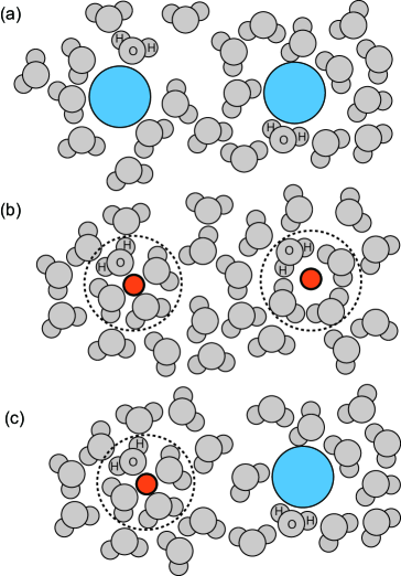
Figure 1: (Color online) Illustration of two ions in close separation in waterCollins (1997). (a) Large-large pair with non-Coulombic attraction. Examples are CsI and CsBr. (b) Small-small ions with non-Coulombic attraction. Examples are NaF and LiF. (c) Small-large (cation-anion) pair with non-Coulombic repulsion. Examples are NaI, LiI, and NaBPh₄. Tendency of cation-anion association is promoted with decreasing $U_{23}^{\rm eff}$.

II.4 Fluctuation variances, charge density structure factor, and Kirwood-Buff integrals

We treat $\delta n_{i}$ as the thermal fluctuations obeying the Gaussian distribution $\propto\exp(-\delta{\cal F}/k_{B}T)$. We can then calculate the fluctuation variances $I_{ij}=\lim_{q\to 0}\langle{n_{i}({\mbox{\boldmath$q$}})n_{j}({\mbox{\boldmath$q$}})^{*}}\rangle/V$, where $L^{-1}\ll q\ll\kappa$ in the limit of large $L$. Here, for any space-dependent variables ${\hat{A}}({\mbox{\boldmath$r$}})$ and $\hat{B}({\mbox{\boldmath$r$}})$, we write $\langle{\hat{A}:\hat{B}}\rangle=\lim_{q\to 0}\langle{A_{\mbox{\boldmath$q$}}{B_{\mbox{\boldmath$q$}}}^{*}}\rangle/V$, where $A_{\mbox{\boldmath$q$}}$ and $B_{\mbox{\boldmath$q$}}$ are the Fourier componentsOnuki (2002). Then, $I_{ij}=\langle{n_{i}:n_{j}}\rangle$. From Eq.(20) we findOkamoto and Onuki (2018)

$$\langle{\phi_{v}:\phi_{v}}\rangle=k_{B}T/n_{\rm w}^{2}f_{11}\cong\epsilon_{\rm in}/n_{\rm w},$$ (26)

$$\langle{\phi_{v}:n_{i}}\rangle=0~{}~{}(i=2,3).$$ (27)

As $q\to 0$, we have $\rho_{\mbox{\boldmath$q$}}\to 0$, so we find

$$I_{22}=I_{33}=I_{23}=n_{\rm s}\chi,$$ (28)

where $n_{\rm s}\chi$ represents the amplitude of the ion density fluctuations. See its thermodynamic expression in Eq.(44). From Eq.(18) we also find the solvent-solvent and solvent-ion fluctuation variances,

$$I_{11}=k_{B}T/f_{11}+(f_{12}+f_{13})^{2}f_{11}^{-2}n_{\rm s}\chi,$$ (29)

$$I_{12}=I_{13}=-(f_{12}+f_{13})f_{11}^{-1}n_{\rm s}\chi\cong-v_{\rm s}^{*}n_{\rm w}n_{\rm s}/2.$$ (30)

In $I_{11}$, the first and second terms are close to $n_{\rm w}\epsilon_{\rm in}$ and $(n_{\rm w}v_{\rm s}^{*})^{2}n_{\rm s}/2$, respectively, for small $n_{\rm s}$. Thus, the second one is dominant for $n_{\rm s}/n_{\rm w}>2\epsilon_{\rm in}/(v_{\rm s}^{*}n_{\rm w})^{2}$ ($\sim 4\times 10^{-4}$ for NaPhB₄ in water), as can be verified in experiments.

It is convenient to rewrite ${\delta{\cal F}_{\rm ion}}$ in Eq.(23) in terms of $\delta n_{\rm e}=\delta n_{2}+\delta n_{3}$ and $\rho=e(\delta n_{2}-\delta n_{3})$ as

$$\frac{\delta{\cal F}_{\rm ion}}{k_{B}T}=\int d{\mbox{\boldmath$r$}}\Big{[}\frac{|\delta n_{\rm e}|^{2}}{8n_{\rm s}\chi}+(U_{22}^{\rm eff}-U_{33}^{\rm eff})\frac{{\delta n_{\rm e}}\rho}{4k_{B}Te}\Big{]}$$

$$\hskip 11.38109pt+\int_{\mbox{\boldmath$q$}}\Big{[}1+w_{\rho}n_{\rm s}+\frac{\kappa^{2}}{q^{2}}\Big{]}\frac{|\rho_{\mbox{\boldmath$q$}}|^{2}}{4e^{2}n_{\rm s}}.$$ (31)

The inverse $\chi^{-1}$ in the first term depends on $n_{\rm s}$ as

$$\chi^{-1}=2-\ell_{B}\kappa/2+2n_{\rm s}U_{\rm eff}/k_{B}T.$$ (32)

The coefficient $w_{\rho}$ in the second term arises from asymmetry between the cations and the anions as

$$w_{\rho}=(U_{22}^{\rm eff}+U_{33}^{\rm eff}-2U_{23}^{\rm eff})/2k_{B}T$$

$$=[U_{22}+U_{33}-2U_{23}-(v_{2}^{*}-v_{3}^{*})^{2}/2\kappa_{\rm w}]/2k_{B}T.$$ (33)

From Eq.(31) the structure factor for the charge density fluctuations $\rho_{\mbox{\boldmath$q$}}$ for $q\ll\kappa$ is given byO’Connell and DeGance (1975); Evans and Sluckin (1980); de Carvalho and Evans (1994); Attard (1993)

$$S_{\rho\rho}(q)=\langle{|\rho_{\mbox{\boldmath$q$}}|^{2}}\rangle/V={2e^{2}n_{\rm s}}/[1+w_{\rho}n_{\rm s}+{\kappa^{2}}/{q^{2}}].$$ (34)

The cross term $\propto\rho\delta n_{\rm e}$ in Eq.(31) gives a higher-order term$(\propto n_{\rm s}^{2}$) in the denominator in Eq.(34). For $1+w_{\rho}n_{\rm s}>0$, the screening length is given by

$$\xi_{\rho}=\kappa^{-1}\sqrt{1+w_{\rho}n_{\rm s}},$$ (35)

which is valid for $\kappa d_{1}\ll 1$ or for $n_{\rm s}\ll 0.02n_{\rm w}\sim 1$ mol$/$L with $d_{1}=3{\rm\AA}$ in water. In Sec.IV, we shall see that $w_{\rho}$ is negative and $|w_{\rho}|$ increases with increasing the cation-anion asymmetry (see Fig.9(d) and Eq.(100)). Thus, $\xi_{\rho}\kappa$ decreases with increasing $n_{\rm s}$ for small $n_{\rm s}$ as observedSmith et al. (2016). A similar decrease was derived in the MSA schemeBlum (1975); Simonin et al. (1996) and in phenomenoological theoriesAttard (1993); Adar et al. (2019) However, $\xi_{\rho}$ increases with increasing $n_{\rm s}$ above 1 mol$/$LSmith et al. (2016); Adar et al. (2019); Coles et al. (2020), as a remarkable effect beyond the scope of this paper.

In Eq.(28) the cations and the anions are indistinguishable. Thus, we define the Kirkwood-Buff integrals (KBIs)Kirkwood and Buff (1951) for the water density $n_{1}$ and the ion density $n_{\rm e}=n_{2}+n_{3}$Kusalik and Patey (1987); Newman (1989); Weerasinghe and Smith (2003); Klasczyk and Knecht (2010); Fyta and Netz (2012); Naleem et al. (2018). Then, Eqs.(28)-(30) give the ion-ion and ion-solvent KBIs:

$$G_{\rm ss}=\langle{n_{\rm e}:n_{\rm e}}\rangle/4n_{\rm s}^{2}-1/2n_{\rm s}=(2\chi-1)/2n_{\rm s},$$ (36)

$$G_{{\rm ws}}=\langle{n_{1}:n_{\rm e}}\rangle/2n_{\rm w}n_{\rm s}=-\chi(f_{12}+f_{13})/n_{\rm w}f_{11}.$$ (37)

Thus, as $n_{\rm s}\to 0$, we have $G_{\rm ss}\propto n_{\rm s}^{-1/2}$ and $G_{{\rm ws}}\cong-{v_{\rm s}^{*}}/{2}$. Note that $G_{{\rm ws}}$ represents exclusion (adsorption) of water molecules around an ion pair for positive (negative) $v_{\rm s}^{*}$.

In their simulation, Naleem et al.Naleem et al. (2018) found growth of $G_{\rm ss}$ at low densities of CaCl₂. Here, we readily derive $G_{\rm ss}=Z_{+}Z_{-}\ell_{B}\kappa/4\langle{n_{\rm e}}\rangle+\cdots$, where the cations and anions have changes $Z_{+}e$ and $-Z_{-}e$, respectively,

III Thermodynamics of electrolytes

In this section, we study the electrolyte thermodynamics using the Helmholtz free energy $F=\lim_{\Lambda\to 0}{\cal F}$. We give remarks on previous research. (i) PitzerPitzer (1973) used the Gibbs free energy $G$. In Appendix B, a scheme of $G$ will be given. (ii) In many papersRobinson and Stokes (2002); Bjerrum (1926); Smith and Dang (1994); Ebeling and Grigo (1982); Levin and Fisher (1996); Degr$\grave{\rm e}$ve and da Silva (1999); Hassan (2008); Adar et al. (2017); Zwanikken and van Roij (2009); Marcus and Hefter (2006); van der Vegt et al. (2016); Fennell et al. (2009), associated ion pairs are treated as dipoles coexisting with unbound ions. However, they appear as ion clusters with finite lifetimes in water. In Appendix A, we will show how our theory is modified by such dipoles at small $n_{\rm s}$. (iii) Since McQuarrie’s paper on fused saltsOlivares and Mcquarrie (1962), many authorsStell (1996); McGahay and Tomozawa (1989); Ebeling and Grigo (1982); Levin and Fisher (1996); Card and Valleau (1970); Romero-Enrique et al. (2000) discussed a gas-liquid phase transition of the ions due to ${f}_{\rm DH}$ in Eq.(5) without solvent-ion interactions, where $a_{2}$ and $a_{3}$ are the ion hardsphere diameters.

III.1 Free energy, chemical potentials, pressure, and thermodynamic derivatives

From Eqs.(3) and (7)-(9). $F$ is expressed as

$$F/V =f_{\rm w}(n_{\rm w})+2k_{B}T[\ln(n_{\rm s}{\lambda}^{3})-1+\nu(n_{\rm w})]n_{\rm s}$$ (38)

$$-k_{B}T\kappa^{3}/12\pi+Un_{\rm s}^{2}.$$

where $\lambda=\sqrt{\lambda_{2}\lambda_{3}}$. This is the expression up to order $n_{\rm s}^{2}$. We introduce the solvent chemical potential $\mu_{\rm w}$ and the salt one $\mu_{\rm s}$ (per cation-anion pair) from $d(F/V)=\mu_{\rm w}dn_{\rm w}+\mu_{\rm s}dn_{\rm s}$ at fixed $T$. The pressure $p=n_{\rm w}\mu_{\rm w}+n_{\rm s}\mu_{\rm s}-F/V$ satisfies the Gibbs-Duhem relation,

$$dp=n_{\rm w}d\mu_{\rm w}+n_{\rm s}d\mu_{\rm s}.$$ (39)

From Eq.(38), $\mu_{\rm w}$, $\mu_{\rm s}$, and $p$ are expanded as

$$\mu_{\rm w}=\mu^{0}_{\rm w}(n_{\rm w})+k_{B}T[2\nu^{\prime}+\ell_{B}\kappa\epsilon^{\prime}/\epsilon]n_{\rm s}+U^{\prime}n_{\rm s}^{2},$$ (40)

$${\mu}_{\rm s}=k_{B}T[2\ln(n_{\rm s}\lambda^{3})+2\nu-\ell_{B}\kappa]+2Un_{\rm s},$$ (41)

$$p=p^{0}_{\rm w}(n_{\rm w})+2k_{B}T(1+n_{\rm w}\nu^{\prime})n_{\rm s}+(U+n_{\rm w}U^{\prime})n_{\rm s}^{2}$$

$$-k_{B}T\kappa^{3}(1-3n_{\rm w}\epsilon^{\prime}/\epsilon)/24\pi,$$ (42)

where $U^{\prime}=\partial U(n_{\rm w})/\partial n_{\rm w}$. We define the chemical potential $\mu^{0}_{\rm w}=\partial f_{\rm w}(n_{\rm w})/\partial n_{\rm w}$ and the pressure $p^{0}_{\rm w}=n_{\rm w}\mu^{0}_{\rm w}-f_{\rm w}$ for pure solvent at density $n_{\rm w}$. They vary significantly even for a small change of $n_{\rm w}$ from $n_{\rm w}\partial\mu^{0}_{\rm w}/\partial n_{\rm w}=\partial p^{0}_{\rm w}/\partial n_{\rm w}=1/n_{\rm w}\kappa_{\rm w}=k_{B}T/\epsilon_{\rm in}$.

Next, the second derivatives of $F/V$ are written as

$$f_{KM}=\frac{\partial^{2}(F/V)}{\partial n_{M}\partial n_{K}}=\frac{\partial\mu_{K}}{\partial n_{M}}\quad(K,M={\rm w},{\rm s}).$$ (43)

Here, $f_{\rm ww}=f_{11}$, $f_{\rm ws}=\sum_{i=2,3}f_{1i}$, and $f_{\rm ss}=\sum_{i,j=2,3}f_{ij}$ in terms of $f_{ij}$ in Eq.(13). Note that the inverse matrix of $\{f_{KM}\}$ is given by $\{\partial n_{K}/\partial\mu_{M}\}$, where $n_{\rm w}$ and $n_{\rm s}$ are functions of $\mu_{\rm w}$ and $\mu_{\rm s}$. The elements of this inverse matrix are the fluctuation variances among $\delta n_{1}$ and $(\delta n_{2}+\delta n_{3})/2$ divided by $k_{B}T$. Thus, Eq.(28) gives

$$n_{\rm s}\chi=k_{B}T(\partial n_{\rm s}/\partial\mu_{\rm s})_{\mu_{\rm w},T}=k_{B}T/[f_{\rm ss}-f_{\rm ws}^{2}/f_{\rm ww}].$$ (44)

Let us examine the isothermal compressibility $\kappa_{T}=-V^{-1}\partial V/\partial p$, where $N_{\rm w}=Vn_{\rm w}$, $N_{\rm s}=Vn_{\rm s}$, and $T$ are fixed in the pressure derivative. In terms of $f_{KM}$ in Eq.(43), its inverse is expressed as

$$\kappa_{T}^{-1}=\sum_{K={\rm w},{\rm s}}n_{K}\frac{\partial p}{\partial n_{K}}=\sum_{K,M={\rm w},{\rm s}}n_{K}n_{M}f_{KM}$$

$$=\kappa_{\rm w}^{-1}+2k_{B}T(1+2n_{\rm w}\nu^{\prime}+n_{\rm w}^{2}\nu^{\prime\prime})n_{\rm s},$$ (45)

where the DH term is of order $n_{\rm s}^{3/2}$ (not written here). For NaCl in water, Millero et al.Millero et al. (1974) found that $({{\kappa_{\rm w}}/{\kappa_{T}}}-1)/n_{\rm s}$ tends to a constant as $n_{\rm s}\to 0$, which was $7n_{\rm w}^{-1}$ at $T=303$ K. Thus, $n_{\rm w}\nu^{\prime\prime}/\nu^{\prime}\sim 5$ from Eq.(45).

The thermodynamic partial volumes are defined by ${\bar{v}}_{K}=(\partial V/\partial N_{K})_{T,p,N_{M}}$ ($M\neq K)$. Since $V$ and $N_{K}=Vn_{K}$ are extensive, they satisfy the sum rule ${\bar{v}}_{\rm w}{n}_{\rm w}+{\bar{v}}_{\rm s}{n}_{\rm s}=1$. At fixed $T$, the relation $dV=\sum_{K}{\bar{v}}_{K}dN_{K}-V\kappa_{T}dp$ then holds yielding $\kappa_{T}dp=\sum_{K}{\bar{v}}_{K}dn_{K}$ and

$${\bar{v}}_{\rm s}=\kappa_{T}(\partial p/\partial n_{\rm s})_{T,n_{\rm w}},\quad{\bar{v}}_{\rm w}=\kappa_{T}(\partial p/\partial n_{\rm w})_{T,n_{\rm s}}.$$ (46)

Here, ${\bar{v}}_{\rm s}$ is defined for a cation-anion pair. As $n_{\rm s}\to 0$, Eqs.(42) and (46) give the infinite-dilution limit,

$${\bar{v}}_{{\rm s}}^{0}=\lim_{n_{\rm s}\to 0}{\bar{v}}_{\rm s}=2\epsilon_{\rm in}(\nu^{\prime}+n_{\rm w}^{-1})=v_{\rm s}^{*}+2k_{B}T\kappa_{\rm w},$$ (47)

where $v_{\rm s}^{*}$ appears in Eq.(21). The difference ${\bar{v}}_{{\rm s}}^{0}-{v}^{*}_{{\rm s}}=2k_{B}T\kappa_{\rm w}$ stems from the ionic partial pressure $2k_{B}Tn_{\rm s}$ and is $0.12n_{\rm w}^{-1}$ in ambient water. It is relevant for small-small ion pairs; for example, $n_{\rm w}{\bar{v}}_{{\rm s}}^{0}=-0.09$ and $n_{\rm w}v_{\rm s}^{*}=-0.21$ for NaF. The values of ${\bar{v}}_{{\rm s}}^{0}$ are listed for various salts in the experimental reportsMillero (1971); Mazzinia and Craig (2017); Millero (1970). Many authorsMillero (1971); Marcus (2011); Hepler (1957); Mukerjee (1960); Padova (1963) introduced single-ion volumes, which are $v_{i}^{*}+k_{B}T\kappa_{\rm w}$ in our notation.

III.2 Salt-doping and apparent partial volumes

In experiments of salt-doping, it follows an apparent partial volume $v_{\rm s}^{\rm ap}$ from the space-filling relationRedlich (1940); Redlich and Meyer (1964); Millero (1971); Robinson and Stokes (2002):

$$n_{\rm w}/n_{\rm w}^{0}+v_{\rm s}^{\rm ap}n_{\rm s}=1,$$ (48)

where $n_{\rm w}^{0}$ is the initial solvent density. The salt density is increased from 0 to $n_{\rm s}$. The simplest example is to fix the volume $V$, where $n_{\rm w}=n_{\rm w}^{0}$, $v_{\rm s}^{\rm ap}=0$, and $\ln\gamma_{\pm}=-\ell_{B}\kappa/2+Un_{\rm s}/k_{B}T$ from Eq.(41) (see Eq.(54) for the definition of $\gamma_{\pm}$).

As a well-known doping method, let a 1:1 electrolyte region be in osmotic equiibrium with a pure solvent region, which are separated by a semipermeable membraneMcMillan and Mayer (1945); Luo and Roux (2010); Okamoto and Onuki (2018). The solvent chemical potential $\mu_{\rm w}$ is commonly given by $\mu_{\rm w}(n_{\rm w},n_{\rm s})=\mu_{\rm w}^{0}(n_{\rm w}^{0})$. From $d\mu_{\rm w}=\sum_{K}f_{\rm wK}dn_{\rm K}=0$, we set up the equation,

$${dn_{\rm w}}/{dn_{\rm s}}=({\partial n_{\rm w}}/{\partial n_{\rm s}})_{\mu_{1},T}=-{f_{{\rm ws}}}/{f_{{\rm ww}}}.$$ (49)

From Appendix C, we find the apparent partial volume,

$$v_{\rm s}^{\rm ap}=v_{\rm s}^{*}(n_{\rm w}^{0})+(\epsilon^{\prime}/\epsilon)\epsilon_{\rm in}\ell_{B}\kappa+n_{\rm s}\partial U_{\rm eff}/\partial p.$$ (50)

We also calculate the osmotic pressure $\Pi=p(n_{\rm w},n_{\rm s})-p_{\rm w}^{0}(n_{\rm w}^{0})$. From $d\Pi=n_{\rm s}d\mu_{\rm s}$ and Eq.(44), we find

$$d\Pi/dn_{\rm s}=n_{\rm s}\sum_{K}f_{\rm sK}(dn_{\rm K}/dn_{\rm s})=k_{B}T/\chi,$$ (51)

which holds for general $n_{\rm s}$. We integrate Eq.(51) using Eq.(32) to obtain

$$\Pi/2k_{B}Tn_{\rm s}=1-\ell_{B}\kappa/6+U_{\rm eff}n_{\rm s}/2k_{B}T.$$ (52)

III.3 Isobaric equilibrium at fixed $p$

Most salt-doping experiments have been performed at a constant pressure $p$Lewis and Randall (1921); Br$\ddot{\rm o}$nsted (1922); Pailthorpe et al. (1984); Robinson and Stokes (2002). In this case, the salt number is increased from $0$ to $N_{\rm s}=Vn_{\rm s}$ with

$$p(n_{\rm w},n_{\rm s})=p_{\rm w}^{0}(n_{\rm w}^{0}),$$ (53)

where $n_{\rm w}^{0}$ is the initial solvent density. We can also fix the total solvent number $N_{\rm w}=Vn_{\rm w}=V_{0}n_{\rm w}^{0}$, where $V_{0}$ is the initial volume. Then, Eq.(48) becomes $V=V_{0}+v_{\rm s}^{\rm ap}N_{\rm s}$. This isobaric $v_{\rm s}^{\rm ap}$ has been measured, where the product $\phi_{\rm v}=v_{\rm s}^{\rm ap}N_{\rm A}$ is called the apparent molal volume with $N_{\rm A}$ being the Avogadro number. In Eq.(B3) in Appendix B, ${\bar{v}}_{\rm s}$ will be expressed in terms of this $v_{\rm s}^{\rm ap}$.

We define the molal mean activity coefficient $\gamma_{\pm}$ by expressing the salt chemical potential $\mu_{\rm s}$ in Eq.(41) as

$$\mu_{\rm s}/2k_{B}T=\nu(n_{\rm w}^{0})+\ln(\lambda^{3}\gamma_{\pm}N_{\rm s}/V_{0}).$$ (54)

We also introduce the molar mean activity coefficientRobinson and Stokes (2002),

$$y_{\pm}=(V/V_{0})\gamma_{\pm}=(1+v_{\rm s}^{\rm ap}N_{s}/V_{0})\gamma_{\pm}.$$ (55)

Then, $\gamma_{\pm}N_{\rm s}/V_{0}=n_{\rm s}y_{\pm}$ in Eq.(54). Setting $\nu(n_{\rm w})\cong\nu(n_{\rm w}^{0})-\nu^{\prime}n_{\rm w}^{0}{\bar{v}}_{{\rm s}}^{0}n_{s}$ in Eq.(41), we obtain

$$\ln\gamma_{\pm}=-\ell_{B}\kappa/2+{\tilde{U}}_{\rm eff}n_{\rm s}/k_{B}T.$$ (56)

At fixed $p$ we use the coefficient ${\tilde{U}}_{\rm eff}$ defined by

$${\tilde{U}}_{\rm eff}=U-({\bar{v}}_{{\rm s}}^{0})^{2}/2\kappa_{\rm w}=U_{\rm eff}-k_{B}T(v_{\rm s}^{*}+{\bar{v}}_{{\rm s}}^{0}),$$ (57)

where $v_{\rm s}^{*}$ in Eq.(25) is replaced by ${\bar{v}}_{{\rm s}}^{0}$ in Eq.(47). It will also appear in the Gibbs free energy in Appendix B. Note that ${\tilde{U}}_{\rm eff}/k_{B}T$ can be known from the data of $(\ln\gamma_{\pm}+\ell_{B}\kappa/2)/n_{\rm s}$, which is slightly negative for LiF ($\sim-2/n_{\rm w}$)Hamann et al. (2007), positive for the the other alkali halide salts, and is largely negative for NaPBh₄ ($\sim-60/n_{\rm w}$)Herrington and Taylor (1982).

We also have $dp=\sum_{K,M}(n_{K}f_{KM})dn_{M}=0$ from Eq.(39). Using Eq.(43), we can set up the equation,

$$\frac{dn_{\rm w}}{dn_{\rm s}}={\bigg{(}}\frac{\partial{n_{\rm w}}}{\partial{n_{\rm s}}}{\bigg{)}}_{p,T}=-\frac{f_{\rm ws}}{f_{\rm ww}}-\frac{k_{B}T/\chi}{n_{\rm w}f_{\rm ww}+n_{\rm s}f_{\rm ws}}.$$ (58)

Here, the second term is $(\partial n_{\rm s}/\partial\mu_{\rm w})_{n_{\rm s},T}(\partial\mu_{\rm w}/\partial n_{\rm s})_{p,T}$. From Appendix C, we find the aparent partial volume,

$${v}_{\rm s}^{\rm ap}={\bar{v}}_{{\rm s}}^{0}(n_{\rm w}^{0})+(\epsilon^{\prime}/\epsilon-1/3n_{\rm w})\epsilon_{\rm in}{\ell}_{B}\kappa+hn_{\rm s}.$$ (59)

The second term is the DH part derived by RedlichRedlich (1940); Redlich and Meyer (1964). The $h$ is called the deviation constant and has been measured (see Table IV in Sec.IV)Millero (1971, 1970); Desnoyers et al. (1969). It is expressed as

$$h=\kappa_{\rm w}{\tilde{U}}_{\rm eff}+\partial{\tilde{U}}_{\rm eff}/\partial p.$$ (60)

We can also derive Eqs.(59) and (60) by expanding $p(n_{\rm w},n_{\rm s})$ in Eq.(42) with respect to $\delta n_{\rm w}=n_{\rm w}-n_{\rm w}^{0}$.

The derivative $d\mu_{\rm w}/dn_{\rm s}=(\partial\mu_{\rm w}/\partial n_{\rm s})_{p,T}$ is given by the second term in Eq.(58) multiplied by $f_{\rm ww}$. Its integration gives $\mu_{\rm w}$, leading to $\mu_{\rm w}=\mu_{\rm w}^{0}-2k_{B}Tn_{\rm s}/n_{\rm w}^{0}+\cdots$ for small $n_{\rm s}$, where $\mu_{\rm w}^{0}=f_{\rm w}^{\prime}(n_{\rm w}^{0})$ is the initial chemical potential of pure solvent. Thus, we define

$$\varphi=[\mu_{\rm w}^{0}(n_{\rm w}^{0})-\mu_{\rm w}(n_{\rm w},n_{\rm s})]/(2k_{B}Tn_{\rm s}/n_{\rm w}).$$ (61)

After some calculations we obtain the expansion,

$$\varphi=1-\ell_{B}\kappa/6+{\tilde{U}}_{\rm eff}n_{\rm s}/2k_{B}T.$$ (62)

This $\varphi$ is called the osmotic coefficient as well as $\Pi/2k_{B}Tn_{\rm s}$ in Eq.(52)Pailthorpe et al. (1984); Robinson and Stokes (2002), but the linear term($\propto n_{\rm s}$) in Eq.(52) is larger than that in Eq.(62) by $({\bar{v}}_{{\rm s}}^{0}-k_{B}T\kappa_{\rm w})n_{\rm s}$.

From ${n_{\rm s}}{d\mu_{\rm s}}/dn_{\rm s}=-{n_{\rm w}}d\mu_{\rm w}/dn_{\rm s}$, we also findKusalik and Patey (1987)

$$1+n_{\rm s}(\partial\ln y_{\pm}/\partial n_{\rm s})_{p,T}=1/[{1+2n_{\rm s}(G_{\rm ss}-G_{{\rm ws}})}],$$ (63)

with the aid of Eqs.(54) and (55). Here, $G_{\rm ss}$ and $G_{{\rm ws}}$ are the KBIs in Eqs.(36) and (37), which satisfy $1+2n_{\rm s}(G_{\rm ss}-G_{\rm ws})=2\chi(1+n_{\rm s}f_{\rm ws}/n_{\rm w}f_{\rm ww})$ from Eq.(44). This relation has been used in simulations to calculate $y_{\pm}$Weerasinghe and Smith (2003); Klasczyk and Knecht (2010); Fyta and Netz (2012); Naleem et al. (2018).

We make some comments. (i) In Appendix B, we will derive Eqs.(59), (60), and (62) from the Gibbs free energy. (ii) Bernard et al.Pailthorpe et al. (1984) related $\varphi$ and $\Pi$ by $\varphi=(1-{\bar{v}}_{{\rm s}}^{0}n_{\rm s})\Pi/2k_{B}Tn_{\rm s}$, where ${\bar{v}}_{{\rm s}}^{0}$ should be replaced by ${\bar{v}}_{{\rm s}}^{0}-k_{B}T\kappa_{\rm w}$ in our theory. (iii) The behavior $\propto\sqrt{n_{\rm s}}$ of the first corrections in $\ln\gamma_{\pm}$ and $\varphi$ is the DH limiting law, which was known empirically before the DH theoryLewis and Randall (1921); Br$\ddot{\rm o}$nsted (1922).

III.4 Expressions in extended Debye-Hückel theory

With increasing $n_{\rm s}$, the lowest DH terms in Eqs.(56), (59), and (62) increase as $\sqrt{n_{\rm s}}$, while the Debye length $\kappa^{-1}$ decreases toward the minimum length ($a_{2}$ or $a_{3}$). However, ${f}_{\rm DH}$ in Eq.(5) is suppressed with increasing $a_{i}\kappa$. Due to this reason, many authors used extended DH expressions to explain experimental dataRobinson and Stokes (2002); Hamann et al. (2007); Guggenheim (1935); Guggenheim and Turgen (1955); Pitzer (1973).

We thus rewrite $\gamma_{\pm}$ in Eq.(56) and $\varphi$ in Eq.(62) asGuggenheim (1935); Guggenheim and Turgen (1955)

$$\ln\gamma_{\pm}=-\frac{1}{4}\ell_{B}\kappa\sum_{i=2,3}\frac{1}{1+a_{i}\kappa}+bn_{\rm s},$$ (64)

$$\varphi=1-\frac{1}{12}\ell_{B}\kappa\sum_{i=2,3}\sigma(a_{i}\kappa)+\frac{1}{2}b^{\prime}n_{\rm s},$$ (65)

where $\sigma(x)=3[x+x/(1+x)-2\ln(1+x)]/x^{3}$ and $\sigma(x)=1-3x/2+\cdots$ for $x\ll 1$. For small $a_{i}\kappa$ we compare Eqs.(64) and (65) and Eqs.(56) and (62) to find

$$b=b^{\prime}\cong{\tilde{V}}_{\rm eff}/k_{B}T.$$ (66)

Here, using ${\tilde{U}}_{\rm eff}$ in Eq.(57) and $u_{ij}^{\rm ex}$ in Eq.(6), we define

$${\tilde{V}}_{\rm eff}={\tilde{U}}_{\rm eff}-\frac{1}{2}\sum_{i,j}u_{ij}^{\rm ex}={\tilde{U}}_{\rm eff}-2\pi k_{B}T\ell_{B}^{2}(a_{2}+a_{3}),$$ (67)

In Appendix D, we will present extended DH forms for $\chi^{-1}$ in Eq.(32) and $v_{\rm s}^{\rm ap}$ in Eq.(59).

Guggenheim and TurgeonGuggenheim (1935); Guggenheim and Turgen (1955) nicely fitted Eqs.(64) and (65) to 1:1 electrolyte data with $b=b^{\prime}$ and $a_{2}=a_{3}=3{\rm\AA}$. They used many data points for each salt. For their choice of $a_{i}$, the relation $a_{i}\kappa\cong\sqrt{m}$ holds, where $m$ is the molality. Many authorsRobinson and Stokes (2002); Hamann et al. (2007); Pitzer (1973) took this practical approach with empirical $b=b^{\prime}$.

Table 1: Data of mean activity coefficient $\gamma_{\pm}$ and osmotic coefficient $\varphi$ for alkali halide salts at molality $0.5$ in ambient waterHamer and Wu (1972). The latter are in (). LiF is insoluble at this density.

	$\mathrm{F}^{-}$	$\mathrm{Cl}^{-}$	$\mathrm{Br}^{-}$	$\mathrm{I}^{-}$
$\mathrm{Li}^{+}$		0.739 (0.964)	0.754 (0.970)	0.824 (1.008)
$\mathrm{Na}^{+}$	0.633 (0.887)	0.681 (0.921)	0.697 (0.932)	0.722 (0.950)
$\mathrm{K}^{+}$	0.670 (0.916)	0.649 (0.900)	0.658 (0.906)	0.676 (0.918)
$\mathrm{Rb}^{+}$	0.701 (0.939)	0.633 (0.891)	0.630 (0.889)	0.627 (0.887)
$\mathrm{Cs}^{+}$	0.721 (0.946)	0.607 (0.873)	0.605 (0.870)	0.601 (0.868)

III.5 Experimental trends and Collins’ rule

Table I gives $\gamma_{\pm}$ and $\varphi$ for alkali halide salts at molality $0.5$ in ambient waterHamer and Wu (1972). We notice the following. (i) For F^-, $\gamma_{\pm}$ and $\varphi$ increase with increasing the cation size. For the other anions, they are smaller for larger cations. (ii) For small cations Li⁺ and Na⁺, $\gamma_{\pm}$ and $\varphi$ increase as the anion size increases. For large cations Rb⁺ and Cs⁺, the tendency is reversed. (iii) For K⁺, they are close for all the anions. Thus, K⁺ ions have a marginal size.

Table 2: Coefficient $b$ in Eq.(64) and ${\tilde{V}}_{\rm eff}/k_{B}T$ from Eqs.(56) and (67) in units of $d_{1}^{3}$. The latter are in (). Use is made of data on the mean activity coefficient for alkali halide salts at molality 0.02 for LiFHamann et al. (2007) and 0.1 for the othersHamer and Wu (1972).

	$\mathrm{F}^{-}$	$\mathrm{Cl}^{-}$	$\mathrm{Br}^{-}$	$\mathrm{I}^{-}$
$\mathrm{Li}^{+}$	-68.0 (-70.4)	22.1 (11.5)	28.3 (17.8)	43.7 (33.2)
$\mathrm{Na}^{+}$	2.1 (-8.4)	14.2 (3.6)	17.4 (6.79)	22.1 (11.5)
$\mathrm{K}^{+}$	9.4 (-1.2)	5.4 (-5.2)	7.8 (-2.8)	11.8 (1.2)
$\mathrm{Rb}^{+}$	15.0 (4.4)	-0.3 (-10.9)	-1.1 (-11.7)	-2.0 (-12.5)
$\mathrm{Cs}^{+}$	24.4 (13.9)	-8.5 (-19.1)	-7.7 (-18.3)	-10.2 (-20.7)

Table II gives $b$ in Eq.(64) and ${\tilde{V}}_{\rm eff}/k_{B}T$ from Eqs.(56) and (67) in units of $d_{1}^{3}=0.9n_{\rm w}^{-1}$, where $a_{2}=a_{3}=3{\rm\AA}$. We use data of $\gamma_{\pm}$ at molality 0.02 for LiFHamann et al. (2007) and 0.1 for the othersHamer and Wu (1972). The molality 0.1 is not very small with $a_{i}\kappa=0.31$, so the numbers of $b$ are larger than those of ${\tilde{V}}_{\rm eff}/k_{B}T$ by 10. Here, $n_{\rm w}U_{\rm eff}/k_{B}T$ is about $-5$ for LiF and is between $50$ and $110$ for the others. These ion-size-dependences are the same as those in Table I. In Fig.2, to illustrate this common trend, we plot $b$ in Table II vs $\alpha_{i}=2R_{i}^{\rm S}/d_{1}$ ($i=2$ for cations and $i=3$ for anions) with $d_{1}=3~{}{\rm\AA}$, using the crystal radii $R_{i}^{\rm S}$ by ShannonShannon (1976).

CollinsCollins (1997) noticed the same pattern in the solubility of alkali halide salts in water as those in Tables I and II. That is, salts of large-small pairs are highly soluble, whereas salts of large-large or small-small pairs are much less soluble. In fact, the solubility is $0.05$, 1, and 20 mol$/$L for LiF, NaF, and LiClStubblefield and Bach (1972); Collins (1997), respectively. He argued that large-small pairs remain apart but cation-anion pairs with comparable sizes tend to be closely connected. Note that the salt solubility is correlated with $U_{23}^{\rm eff}$.

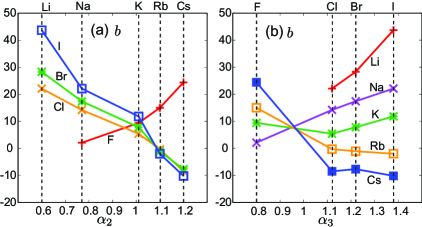
Figure 2: (Color online) Coefficient $b$ in Table II vs radius ratios ($\alpha_{2}$ for cations in (a) and $\alpha_{3}$ for anions in (b)), where $b$ appears in the activity coefficient in Eq.(64). Here, Collins’ rule holds.

For NaBPh₄Herrington and Taylor (1982), the numbers from the two methods in Table II are $-120.7~{}(-130.5)$ at molality $0.09$, leading to $U_{\rm eff}\sim{\tilde{U}}_{\rm eff}\sim-60k_{B}T/n_{\rm w}$. For this salt, the two terms in Eq.(25) are both about $1800k_{B}T/n_{\rm w}$ from $v_{3}^{*}\cong 15/n_{\rm w}$Millero (1970) and their difference $U_{\rm eff}$ is much smaller ($\sim 3\%$).

If the cations and/or the anions are large, $U_{\rm eff}$ is largely negative from Eq.(25). In such cases, a thermodynamic instability occursOkamoto and Onuki (2018) if $n_{\rm s}$ exceeds a spinodal density $n_{\rm s}^{\rm spi}$ determined by $\chi^{-1}=0$. For $n_{\rm w}|U_{\rm eff}|/k_{B}T\gg 20$ in ambient water, the DH term is negligle in Eq.(32), so

$$n_{\rm s}^{\rm spi}\sim k_{B}T/|U_{\rm eff}|.$$ (68)

For NaBPh₄, $n_{\rm s}^{\rm spi}$ is on the order of its solubility ($=1.4$ mol$/$L$=0.025n_{\rm w}$). In this instability, the ions aggregate as solvophobic spinodal decompositionStell (1996); Onuki (2002); Glasbrenner and Weing$\ddot{\rm a}$rtner (1989). However, ion association can trigger precipitate formation in metastable solutions, which is the case for alkali halide salts in waterJoung and Cheatham-III (2009); Aragones et al. (2012); Yagasaki et al. (2020). For LiF, its solubility ($=0.14$ mol$/$L $=0.002n_{\rm w}$) is exceptionally small ($\ll n_{\rm s}^{\rm spi}$). On the other hand, in aqueous mixture solvents, phase separation can be induced even at slight doping of a strongly hydrophilic saltOkamoto and Onuki (2010); Onuki and Okamoto (2011).

III.6 Electrostriction from Born theory

Let us consider the hydration part of the ion chemical potentials due to the ion-dipole interaction, written as $k_{B}T\nu_{i}^{\rm B}$. In the simple continuum theoryBorn (1920); Millero (1971); Marcus (2011), it is the integral of the electrostatic energy density $\epsilon E(r)^{2}/8\pi$ in the region $r>R_{i}$, where $E(r)=\pm e/\epsilon r^{2}$ is the electric field at distance $r$ from the ion and $R_{i}$ is called the Born radius. Using the bulk dielectric constant $\epsilon$, we find

$$k_{B}T\nu_{i}^{\rm B}(n_{\rm w})=(e^{2}/2R_{i})(1/\epsilon-1)\quad(i=2,3),$$ (69)

where the contribution without polarization is subtracted. We assume that $R_{i}$ is independent of $n_{\rm w}$, while $\epsilon$ depends on it as in Eq.(17). From Eq.(19) the electrostriction part of $v_{i}^{*}$ is given by

$$v_{i}^{\rm B}=\epsilon_{\rm in}d\nu_{i}^{\rm B}/dn_{\rm w}=-\epsilon_{\rm in}\ell_{B}\epsilon^{\prime}/(2\epsilon R_{i}),$$ (70)

which is rewritten as $(e^{2}/2R_{i})\partial\epsilon^{-1}/\partial p$, as was first derived by Drude and NernstDrude and Nernst (1894). We also assume homogeneity of the local solvent chemical potential around each ionOnuki (2006); Landau and Lifshitz (1984). We then find the solvent density increase,

$$\delta n_{\rm w}(r)=n_{\rm w}^{2}\kappa_{\rm w}\epsilon^{\prime}E(r)^{2}/8\pi=-n_{\rm w}v_{i}^{\rm B}R_{i}/(4\pi r^{4}),$$ (71)

whose integration ($r>R_{i}$) is $-n_{\rm w}v_{i}^{\rm B}$ as it should be the case. In ambient water, we have $n_{\rm w}v_{i}^{\rm B}\cong-0.24/R_{i}$ and $\delta n_{\rm w}(r)/n_{\rm w}\cong 0.51/r^{4}$ with $R_{i}$ and $r$ in units of $\rm\AA$. where $\delta n_{\rm w}(r)$ grows unrealistically around small ions.

The Born expressions are very approximate. In water, dielectric saturation occurs and $\epsilon$ nonlinearly decreases in the immediate vicinity of ionsPadova (1963)^, In fact, Eq.(70) cannot be well fitted to the electrostriction dataMarcus (2011) if $R_{i}$ is equated with the radius calculated from the crystal lattice constantsShannon (1976). For example, Mazzini and CraigMazzinia and Craig (2017) estimated the electrostriction part of ${\bar{v}}_{{\rm s}}^{0}$ in Eq.(47) as $-13.0$ cm${}^{3}/$mol $=-0.72/n_{\rm w}$ for NaCl. This size is twice as large as that from Eq.(70) if we set $R_{2}\sim 1{\rm\AA}$ for Na⁺ and $R_{3}\sim 2{\rm\AA}$ for Cl^-. Thus, if we use the Born theory with the bulk $\epsilon$ to explain the electrostriction data, we should treat $R_{i}$ as a short, effective radius (see Eq.(86)).

In addition, the static dielectric constant $\epsilon$ depends on $n_{\rm s}$ as $\epsilon(n_{\rm w},n_{\rm s})/\epsilon(n_{\rm w},0)\cong 1-g_{1}n_{\rm s}$, where $g_{1}n_{\rm w}\sim 10$ for alkali hallidesHess et al. (2006b); Wei et al. (1992); Buchner et al. (1999); Levy et al. (2013). This indicates that $1/\epsilon$ in Eq.(69) should be changed to $(1+g_{1}n_{\rm s})/\epsilon(n_{\rm w},0)$, which yields an additional positive contribution to $U_{\rm eff}$Vincze et al. (2010). In this paper, we neglect such an indirect repulsive interaction.

IV Model calculations

To make numerical analysis, we combine the MCSL modelMansoori et al. (1971), the attractive part of the Lennard-Jones (LJ) potentialsTalanquer et al. (2001), and the Born chemical potentialsBorn (1920). Introducing the hardsphere diameters $d_{1}$, $d_{2}$, and $d_{3}$ for the solvent, the cations, and the anions, respectively, we vary the diameter ratios,

$$\alpha_{i}=d_{i}/d_{1}.$$ (72)

The steric interaction sensitively depends on whether $\alpha_{2}$ and $\alpha_{3}$ are larger or smaller than 1. In the following, large and small ions are roughly those with $\alpha_{i}\gtrsim 1.2$ and $\alpha_{i}\lesssim 0.8$, respectively.

IV.1 Local free energy density $f$

The free energy density $f$ in Eq.(3) is given by

$$f=k_{B}T\sum_{i=1,2,3}n_{i}[\ln(n_{i}\lambda_{i}^{3})-1]+f_{\rm DH}+f_{\rm h}+f_{\rm a}+f_{\rm B},$$ (73)

where the first term is the ideal-gas part and $f_{\rm DH}$ is the DH free energy density in Eq.(5). The third term $f_{\rm h}$ is the MCSL steric part written up to second order in $n_{2}$ and $n_{3}$ as

$$f_{\rm h}=f_{\rm h}^{0}(n_{1})+k_{B}T\sum_{i=2,3}\nu_{i}^{h}n_{i}+\frac{1}{2}\sum_{i,j=2,3}U_{ij}^{h}n_{i}n_{j},$$ (74)

where $f_{h}^{0}$ is given by the Carnahan-Starling formCarnahan and Starling (1969),

$$f_{h}^{0}=k_{B}Tn_{1}(4-3\eta_{1})\eta_{1}/(1-\eta_{1})^{2},$$ (75)

with $\eta_{1}=v_{1}n_{1}$ with $v_{1}=\pi d_{1}^{3}/6$ being the hardcore volume of a solvent particle. See Appendix E for expressions of $\nu_{i}^{h}$ and $U_{ij}^{h}$. The fourth term $f_{\rm a}$ represents the attractive interaction assuming the van der Waals form,

$$f_{\rm a}=-\frac{1}{2}\sum_{i,j=1,2,3}w_{ij}n_{i}n_{j}.$$ (76)

The coefficients $w_{ij}$ $(i,j=1,2,3)$ are constants given by

$$w_{ij}=({4\sqrt{2}\pi}/{9})\epsilon_{ij}(d_{i}+d_{j})^{3},$$ (77)

where $\epsilon_{ij}$ are interaction energies in the LJ potentialsTalanquer et al. (2001). From Eq.(69) the hydration part $f_{\rm B}$ is written as

$$f_{\rm B}=k_{B}T\sum_{i=2,3}\nu_{i}^{\rm B}(n_{1})n_{i}.$$ (78)

The free energy density of pure solvent is given byCarnahan and Starling (1972)

$$f_{\rm w}(n_{1})=k_{B}Tn_{1}(\ln(n_{1}\lambda_{1}^{3})-1]+f_{h}^{0}(n_{1})-\frac{1}{2}w_{11}n_{1}^{2}.$$ (79)

The incompressibility parameter $\epsilon_{\rm in}$ in Eq.(10) becomes

$$\epsilon_{\rm in}=[1/\epsilon_{\rm in}^{h}-n_{1}{w_{11}}/{k_{B}T}]^{-1},$$ (80)

where $\epsilon_{\rm in}^{h}$ is the hardcore part. Its iverse is written asCarnahan and Starling (1969)

$$1/\epsilon_{\rm in}^{h}=1+{2\eta_{1}(4-\eta_{1})}/{(1-\eta_{1})^{4}},$$ (81)

where the second term grows for $\eta_{1}\gtrsim 0.5$. For water, the hydrogen bonding yields a high critical temperature ($647.1$K), so we need a relatively large $w_{11}$ to make the phase diagram from $f_{\rm w}$ mimic that of waterOkamoto and Onuki (2018). Thus, we introduce the attraction parameter of the solvent,

$$w_{\rm a}=\epsilon_{\rm in}/\epsilon_{\rm in}^{h}-1=\epsilon_{\rm in}n_{1}w_{11}/k_{B}T,$$ (82)

which is of order 1 for ambient water as its speciality.

We set $d_{1}$ and $\epsilon_{11}$ in $f_{\rm w}$ in Eq.(79) equal to

$$d_{1}=3\,\mathrm{\AA},\quad\epsilon_{11}/k_{B}=412.72\,\mathrm{K}.$$ (83)

For ambient water ($T=300\,\mathrm{K}$ and $p=1\,\mathrm{atm}$), these give the experimental compressibility $\kappa_{\rm w}=4.5\times 10^{-4}$ MPa^-1. We also obtain $n_{1}=0.857/d_{1}^{3}=31.7$nm^-3, which is slightly smaller than the experimental one $=33.3$ nm^-3. Then, $1/\epsilon_{\rm in}^{h}=35.5$ and $n_{1}{w_{11}}/k_{B}T=18.6$. Thus,

$$\eta_{1}=v_{1}n_{1}=0.448,\quad\epsilon_{\rm in}=0.059,\quad w_{\rm a}=1.10.$$ (84)

PreviouslyOkamoto and Onuki (2016, 2018, 2015), we assumed $\epsilon_{11}/k_{B}=588.76$ K to obtain the saturated vapor pressure of water ($=0.031$ atm) at $T=300$ K. As regards the dielectric constant, we set $\epsilon=80$ and $n_{1}\epsilon^{\prime}/\epsilon=1.1$ in accord with Eq.(17).

The other LJ energies in Eq.(77) are given by

$$\epsilon_{1i}/k_{B}=287.3,\mathrm{K},~{}\epsilon_{ij}/k_{B}=200,\mathrm{K}~{}~{}(i,j=2,3),$$ (85)

which are smaller than $\epsilon_{11}/k_{B}$ and satisfy the Lorentz-Berthelot relationsHansen and McDonald (1986) $\epsilon_{ij}=\sqrt{\epsilon_{ii}\epsilon_{jj}}$. For simplicity, we set $\epsilon_{12}=\epsilon_{13}$ not differentiating the properties of cations and anions in water, so we can exchange $\alpha_{2}$ and $\alpha_{3}$ in our results. In molecular dynamics simulation of aqueous electrolytesJoung and Cheatham-III (2009); Aragones et al. (2012); Yagasaki et al. (2020), the pair potentials among ions and water molecules depend on the ion species.

As discussed in Sec.IIIF, to be consistent with the electrostriction data, the Born radii $R_{i}$ should be smaller than the hardsphere radii $d_{i}/2$. In this paper, we set

$$R_{i}=0.2d_{i}\quad(i=2,3).$$ (86)

Then, we have $v_{i}^{*}<0$ for $\alpha_{i}<0.72$ (see Fig.3(a)). If $R_{i}=0.4d_{i}$, we have $v_{i}^{*}<0$ for $\alpha_{i}<0.58$.

IV.2 Ion volume and interaction coefficients

The solvation coefficient $\nu_{i}(n_{1})$ in Eq.(3) consists of three parts as $\nu_{i}(n_{1})=\nu_{i}^{h}-w_{1i}n_{1}/k_{B}T+\nu_{i}^{\rm B}$. Then, from Eq.(19), the ion volume is written as

$$v_{i}^{*}=v_{i}^{h}+v_{i}^{\rm LJ}+v_{i}^{\rm B}.$$ (87)

The MCSL part $v_{i}^{h}=\epsilon_{\rm in}d\nu_{i}^{h}/dn_{1}$ tends to $v_{1}\alpha_{i}^{3}$ for large $\alpha_{1}$ (see Eq.(E4) in Appendix E for its expression). With Eqs.(83)-(86), the LJ part $v_{i}^{\rm LJ}=-{\epsilon_{\rm in}w_{1i}}/{k_{B}T}$ and the Born part $v_{i}^{\rm B}$ in Eq.(70) behave as

$$v_{i}^{\rm LJ}/d_{1}^{3}=-0.11(1+\alpha_{i})^{3},\quad v_{i}^{\rm B}/d_{1}^{3}=-0.44/\alpha_{i}.$$ (88)

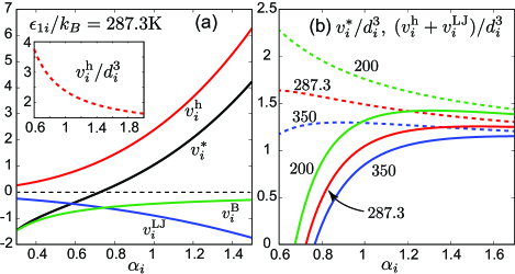
Figure 3: (Color online) (a) Infinite-dilution ion volume $v_{i}^{*}$ (black) composed of $v_{i}^{h}$ (red), $v_{i}^{\rm LJ}$ (blue), and $v_{i}^{\rm B}$ (green) in units of $d_{1}^{3}$ together with $v_{i}^{h}/d_{i}^{3}$ (inset) as functions of $\alpha_{i}=d_{i}/d_{1}$. (b) Ratios $v_{i}^{*}/d_{i}^{3}$ (bold line) and $(v_{i}^{h}+v_{i}^{\rm LJ})/d_{i}^{3}$ (broken line) for $\epsilon_{1i}/k_{B}=200,287.5$, and $350$K. In the other figures, $\epsilon_{1i}/k_{B}=287.5$K.

In Fig.3(a), we examine the three ion-volume parts. For $\alpha_{i}\lesssim 0.5$, we have $v_{i}^{*}\sim v_{i}^{\rm B}<0$. For $\alpha_{i}>1$, both $v_{i}^{h}$ and $v_{i}^{\rm LJ}$ grow as $\alpha_{i}^{3}$, where $v_{i}^{\rm B}$ is negligible. In (b), we plot the ratios $v_{i}^{*}/d_{i}^{3}$ and $(v_{i}^{h}+v_{i}^{\rm LJ})/d_{i}^{3}$ for $\epsilon_{1i}/k_{B}=$200, 287.5, and $350$K, which decrease with increasing $\epsilon_{1i}$. For $\alpha_{i}\gtrsim 1.2$, we can neglect $v_{i}^{\rm B}$ and find

$${v_{i}^{*}}\cong{v_{1}}(1+w_{\rm a})\alpha_{i}^{3}.$$ (89)

See Eq,(E4) and the sentences below it.

To understand the overall behavior of $v_{i}^{*}$, we give a simple interpolation formula,

$$v_{i}^{*}/d_{1}^{3}\cong D_{\rm L}\alpha_{i}^{3}-D_{\rm B}/\alpha_{i},$$ (90)

Here, $D_{\rm L}=\pi(1+w_{\rm a})/6=1.1$ from Eq.(89) and $D_{\rm B}=\epsilon_{\rm in}\ell_{B}\epsilon^{\prime}/(0.4d_{1}^{4}\epsilon)=0.44$ from Eqs.(70) and (86). If $v_{i}^{*}=0$, Eq.(90) yields $\alpha_{i}=0.80$, while our full equations give $\alpha_{i}=0.72$ in Fig.3(a). Previously, some authorsHepler (1957); Mukerjee (1960); Padova (1963); Millero (1971); Marcus (2011) wrote the ion volume ($=v_{i}^{*}+k_{B}T\kappa_{\rm w}$) in the form $A_{\rm I}(2r)^{3}-B_{\rm I}/r$, where $r$ is a certain ion radius with $A_{\rm I}$ and $B_{\rm I}$ being constants. They set $A_{\rm I}\cong 1.0$ in agreement with our $D_{\rm L}=1.1$ (if their $r$ is assumed to be close to the crystal radius).

We next show the salient features of the interaction coefficients. From Eq.(5) $U_{ij}$ in Eq.(3) and $U_{ij}^{\rm eff}$ in Eq.(24) include $u_{ij}^{\rm ex}$ in Eq.(6). We calculate the excess parts,

$$V_{ij}=U_{ij}-u_{ij}^{\rm ex},\quad V_{ij}^{\rm eff}=U_{ij}^{\rm eff}-u_{ij}^{\rm ex},$$

$$V_{\rm eff}=U_{\rm eff}-\frac{1}{2}\sum_{i,j}u_{ij}^{\rm ex}.$$ (91)

We have introduced ${\tilde{V}}_{\rm eff}$ in Eq.(67). From Eq.(73) $V_{ij}$ consist of the MCSL and LJ parts as $V_{ij}=U_{ij}^{h}-w_{ij}$.

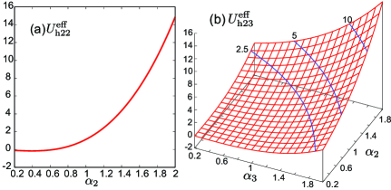
Figure 4: (Color online) (a) ${U_{h22}^{\rm eff}}$ vs $\alpha_{2}$ and (b) ${U_{h23}^{\rm eff}}$ in the $\alpha_{2}$-$\alpha_{3}$ plane in units of ${d_{1}^{3}k_{B}T}$, where $\eta_{1}=0.448$ and $\epsilon_{\rm in}^{h}=0.028$. These are the effective interaction coefficients in Eq.(92) for purely steric hardsphere mixtures in the MCSL model.

We consider the purely steric hardsphere parts of $U_{ij}^{\rm eff}$:

$$U_{hij}^{\rm eff}=U_{ij}^{h}-k_{B}Tn_{1}\epsilon_{\rm in}^{h}(d\nu_{i}^{h}/dn_{1})(d\nu_{j}^{h}/dn_{1}),$$ (92)

which will be explicitly calculated in Appendix E. In Fig. 4, we display ${U_{h22}^{\rm eff}}/d_{1}^{3}k_{B}T$ and ${U_{h23}^{\rm eff}}/d_{1}^{3}k_{B}T$. The former depends on $\alpha_{2}$ only, being nearly zero for $\alpha_{2}<1$ and about 15 for $\alpha_{2}\sim 2$. The latter is nearly zero for $\alpha_{2}<1$ and $\alpha_{3}<1$ and are about 10 for $\alpha_{2}\sim\alpha_{3}\sim 1.8$. The two terms in Eq.(92) are both of order $1200d_{1}^{3}k_{B}T$ for $\alpha_{2}\sim\alpha_{3}\sim 1.8$, so they largely cancel. Thus, $U_{hij}^{\rm eff}$ are smaller than the other contributions with significant attractive and hydration interactions.

Neglecting $U_{hij}^{\rm eff}$ in $V_{ij}^{\rm eff}$, we find some simple limiting behaviors. If $\alpha_{2}$ and $\alpha_{3}$ are both large, we obtain

$$V_{ij}^{\rm eff}/k_{B}Tv_{1}\cong-\alpha_{i}^{3}\alpha_{j}^{3}(w_{\rm a}+w_{\rm a}^{2})/\epsilon_{\rm in},$$ (93)

which are largely negative since $\epsilon_{\rm in}\ll 1$. Thus, salts with large-large ion pairs are hardly soluble in water. This is related to the hydrophobic assembly in water, which has been discussed for uncharged large particlesChandler (2005). Furthermore, if $\alpha_{2}$ is small and $\alpha_{3}$ is large, we obtain

$$V_{23}^{\rm eff}/k_{B}Tv_{1}\cong-v_{2}^{*}\alpha_{3}^{3}(1+w_{\rm a})n_{1}/\epsilon_{\rm in},$$ (94)

which is largely positive for $v_{2}^{*}<0$. Such asymmetric salts are considerably soluble in waterCollins (1997).

The cancellation of the two hrdsphere parts in Eqs.(24) and (92) is a general feature. It is already indicated by the $\gamma_{\pm}$-data of NaBPh₄Herrington and Taylor (1982) (see Sec.IIIE). For a neutral solute, Cerdeiri$\rm{\tilde{n}}$a and WidomCerdeiri$\rm{\tilde{n}}$a and Widom (2016) calculated the two terms in Eq.(1) with a smaller difference (see their Fig.3).

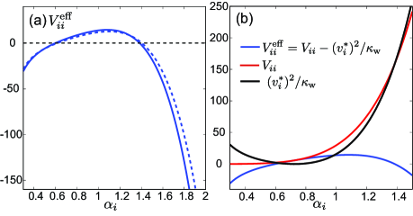
Figure 5: (Color online) (a) Diagonal (cation-cation or anion-anion) component $V_{ii}^{\rm eff}=V_{ii}-(v_{i}^{*})^{2}/\kappa_{\rm w}$ in Eq.(91) vs $\alpha_{i}$ in units of $k_{B}Td_{1}^{3}$. Its approximation in Eq.(99) is also plotted (broken line). (b) Comparison of $V_{ii}^{\rm eff}$ (blue), $V_{ii}$ (red), and $(v_{i}^{*})^{2}/\kappa_{\rm w}$ (black). For large $\alpha_{i}$, the latter two parts grow but mostly cancel, leading to negative $V_{ii}^{\rm eff}$.

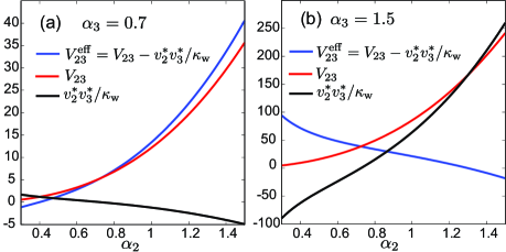
Figure 6: (Color online) Off-diagonal (cation-anion) components $V_{23}^{\rm eff}$ (blue), $V_{23}$ (red), and $v_{2}^{*}v_{3}^{*}/\kappa_{\rm w}$ (black) in units of $k_{B}Td_{1}^{3}$ as functions of $\alpha_{2}$, where $\alpha_{3}$ is (a) $0.7$ and (b) $1.5$. Here, $v_{2}^{*}v_{3}^{*}/\kappa_{\rm w}$ is relatively small in (a), while it is largely negative for $\alpha_{2}<0.6$ and largely positive for $\alpha_{2}>1.2$ in (b).

IV.3 Numerical results of $V_{ij}^{\rm eff}$

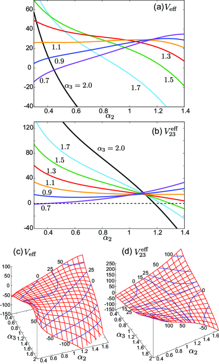
Figure 7: (Color online) (a) $V_{\rm eff}$ and (b) $V_{23}^{\rm eff}$ in units of $k_{B}Td_{1}^{3}$ vs $\alpha_{2}$ for $\alpha_{3}=0.7$, $0.9$, $1.1$, $1.3$, $1.5$, and $2.0$. Displayed also are bird-eye views of (c) $V_{\rm eff}$ and (d) $V_{23}^{\rm eff}$ in the region $0.35<\alpha_{2}<1.7$ and $0.35<\alpha_{3}<2$. They are negative for small-small and large-large pairs, but are positive for small-large pairs (see two peaks)Collins (1997). In (a), the curves decrease into negative regions rapidly for $\alpha_{3}>1.5$ due to diagonal $V_{ii}^{\rm eff}$. The lines of $\alpha_{3}=1.1$ in (a) and (b) are nearly horizontal in the displayed range, which correspond to the contour lines of height 25 in (c) and height 15 in (d).

We present some numerical results. In Fig.5(a), the diagonal component $V_{ii}^{\rm eff}$ in Eq.(91) is plotted vs $\alpha_{i}$, which is independent of $\alpha_{j}$ ($j\neq i$). It is positive in the range $0.60<\alpha_{i}<1.38$ and is negative outside it decreasing as $-{\rm const.}\alpha_{i}^{6}$ for $\alpha_{i}>1.5$. We also plot its approximation to be presented in Eq.(98). In (b), we plot $V_{ii}^{\rm eff}$, $V_{ii}$, and $(v_{i})^{2}/\kappa_{\rm w}$ vs $\alpha_{i}$. For $\alpha_{i}>1.2$, the latter two are large and close. For $\alpha_{i}<0.5$, we have $V_{ii}^{\rm eff}\cong-(v_{i}^{\rm B})^{2}/\kappa_{\rm w}$.

In Fig.6, we show the off-diagonal components $V_{23}^{\rm eff}$, $V_{23}$, and $v_{2}^{*}v_{3}^{*}/\kappa_{\rm w}$ vs $\alpha_{2}$ at fixed $\alpha_{3}$. Here, $v_{2}^{*}v_{3}^{*}/\kappa_{\rm w}$ behaves very differently for (a) $\alpha_{3}=0.7$ and (b) $\alpha_{3}=1.5$ changing its sign at $\alpha_{2}=0.72$. In (a), $V_{23}^{\rm eff}$ and $V_{23}$ are close and monotonically increase with increasing $\alpha_{2}$, where $V_{23}^{\rm eff}=0$ at $\alpha_{2}=0.40$. In (b), $V_{23}^{\rm eff}$ monotonically decreases with increasing $\alpha_{2}$ and is negative for $\alpha_{2}>1.30$, where $V_{23}$ and $v_{2}^{*}v_{3}^{*}/\kappa_{\rm w}$ largely cancel.

In Fig.7, we display $V_{\rm eff}$ and $V_{23}^{\rm eff}$ as functions of $\alpha_{2}$ and $\alpha_{3}$, whose behaviors change abruptly as $\alpha_{2}$ or $\alpha_{3}$ changes across 1. (i) They are largely positive for $\alpha_{2}<1<\alpha_{3}$ or $\alpha_{3}<1<\alpha_{2}$. but are negative if both $\alpha_{2}$ and $\alpha_{3}$, are large or small. The $V_{\rm eff}$ is mostly close to ${\tilde{V}}_{\rm eff}$ in Eq.(67). (ii) They increase (decrease) with increasing $\alpha_{2}$ for small $\alpha_{3}<1$ (large $\alpha_{3}>1$). See the same tendency in Table II and Fig.2 for alkali hallide salts. (iii) The lines of $\alpha_{3}=1.1$ in (a) and (b) are nearly horizontal in the displayed $\alpha_{2}$ range. This explains the marginal behavior of K⁺. In Appendix F, we will explain mathematically why $V_{\rm eff}$ and $V_{23}^{\rm eff}$ change their dependence on $\alpha_{2}$ at $\alpha_{3}\sim 1$.

Table 3: Example of interaction coefficients $V_{ij}$, $V_{ij}^{\rm eff}$, and $V_{\rm eff}$ in units of $k_{B}Td_{1}^{3}$ for small-large ion pair.

$\alpha_{2}$	$\alpha_{3}$	$V_{22}$	$V_{22}^{\rm eff}$	$V_{23}$	$V_{23}^{\rm eff}$	$V_{33}$	$V_{33}^{\rm eff}$	$V_{\rm eff}$
0.7	2	4.86	4.76	78.2	89.6	1108	-291	-53.8

Table III gives $V_{ij}$, $V_{ij}^{\rm eff}$, and $V_{\rm eff}$ for $(\alpha_{2},\alpha_{3})=(0.7,2)$, where $v_{2}^{*}/d_{1}^{3}=-0.080$, and $v_{3}^{*}/d_{1}^{3}=9.83$. In this case, $V_{33}$ and $(v_{3}^{*})^{2}/\kappa_{\rm w}$ are very large and close, leading to $V_{23}^{\rm eff}\sim 90$ and $V_{\rm eff}\sim-50$ in units of $k_{B}Td_{1}^{3}$. For NaBPh₄, we expect similar behavior (see Sec.IIIE).

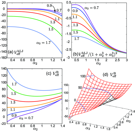
Figure 8: (Color online) (a) Non-Born coefficient $V_{\rm eff}^{\rm hLJ}$ in Eq.(96), (b) $V_{\rm eff}^{\rm hLJ}/(1+\gamma^{2})$ with $\gamma=\alpha_{2}^{3}+\alpha_{3}^{3}$, and (c) Born coefficient $V_{\rm eff}^{\rm B}$ in Eq.(95) as functions of $\alpha_{2}$ for $\alpha_{3}=0.7,0.9,1.1,1.3,1.5$, and $1.7$. Shown in (d) is $V_{\rm eff}^{\rm B}$ in the $\alpha_{2}$-$\alpha_{3}$ plane. These are in units of $k_{B}Td_{1}^{3}$.

IV.4 Role of hydration for small-large pairs

As in Eq.(94), the interplay of the steric and hydration effects leads to the unique behavior of small-large ion pairs. In $V_{\rm eff}$ in Eq.(91), it give rise to

$$V_{\rm eff}^{\rm B}=|v_{\rm B}|(2v_{\rm s}^{*}+|v_{\rm B}|)/2\kappa_{\rm w}$$ (95)

where $v_{\rm B}=v_{2}^{\rm B}+v_{3}^{\rm B}<0$. We then define the non-Born coefficients without hydration as

$$V_{\rm eff}^{\rm hLJ}=V_{\rm eff}-V^{\rm B}_{\rm eff}.$$ (96)

In Fig.8, we examine $V_{\rm eff}^{\rm B}$ and $V_{\rm eff}^{\rm hLJ}$. In (a) and (b), $V_{\rm eff}^{\rm hLJ}$ is largely negative for $\gamma=\alpha_{2}^{3}+\alpha_{3}^{3}>1$ and is small for $\gamma<1$. It is simply approximated by $V_{\rm eff}^{\rm hLJ}/d_{1}^{3}k_{B}T\cong-A\gamma^{2}/2$ with $A=5.0$. On the other hand, in (c) and (d), $V_{\rm eff}^{\rm B}$ is largely positive for small-large pairs and is negative for small-small pairs.

We can devise a simple approximate expression for $V_{\rm eff}$ in terms of $\gamma=\alpha_{2}^{3}+\alpha_{3}^{3}$ and $\zeta=1/\alpha_{2}+1/\alpha_{3}$ as

$$V_{\rm eff}/d_{1}^{3}k_{B}T\cong B\gamma\zeta-C\zeta^{2}/2-A\gamma^{2}/2,$$ (97)

where we use Eq.(90). Here, $B=D_{\rm B}D_{\rm L}d_{1}^{3}n_{1}/\epsilon_{\rm in}=7.0$, $C=BD_{\rm B}/D_{\rm L}=2.8$, and $A=5$. In the same manner, we express the cmponents $V_{ii}^{\rm eff}$ and $V_{23}^{\rm eff}$ as

$$V_{ii}^{\rm eff}/d_{1}^{3}k_{B}T\cong 2B\alpha_{i}^{2}-C/\alpha_{i}^{2}-A\alpha_{i}^{6},$$ (98)

$$V_{23}^{\rm eff}/d_{1}^{3}k_{B}T\cong[B(\alpha_{2}^{4}+\alpha_{3}^{4})-C]/\alpha_{2}\alpha_{3}-A\alpha_{2}^{3}\alpha_{3}^{3}.$$ (99)

These simple expressions can well describe the overall behaviors of $V_{ij}^{\rm eff}$ in Figs.5-7.

IV.5 Numerical results of $\chi^{-1}$, $w_{\rho}$, $G_{\rm ee}$, $\ln\gamma_{\pm}$, and $\varphi$

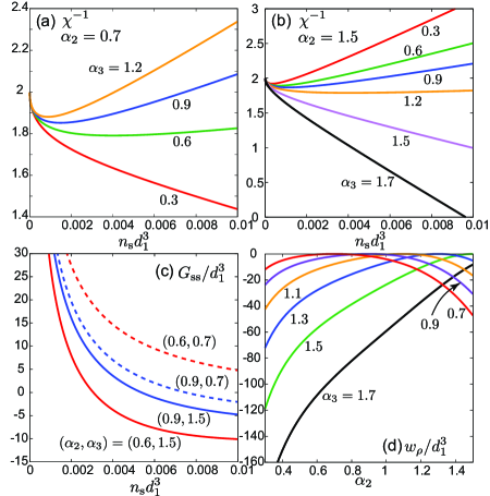
Figure 9: (Color online) $\chi^{-1}$ vs $n_{\rm s}d_{1}^{3}$ for $\alpha_{3}=0.3,0.6,0.9$, and 1.2, where $\alpha_{2}$ is (a) $0.7$ and (b) 1.5 and use is made of Eq.(D1). (c) $w_{\rho}d_{1}^{3}$ in Eq.(33) vs $\alpha_{2}$ for $\alpha_{3}=0.7+0.2m$ ($0\leq m\leq 5$), (d) $G_{\rm ss}/d_{1}^{3}$ in Eq.(36) vs $n_{\rm s}d_{1}^{3}$. for ($\alpha_{2},\alpha_{3})=(0.6,0.7),(0.9,0.7),(0.9,1.5)$, and ($0.6,1.5)$. Here, the upper bound of the salt density $n_{\rm s}$ is $0.01/d_{1}^{3}\sim 0.5$ mol$/$L.

In Fig.9, setting (a) $\alpha_{2}=0.7$ and (b) 1.5, we plot $\chi^{-1}$ vs $n_{\rm s}d_{1}^{3}$($=0.86n_{\rm s}/n_{1}$) for various $\alpha_{3}$, We use its extended DH form (D1) with $a_{2}=a_{3}=3~{}{\rm\AA}$, where $n_{\rm s}\chi$ represents the ionic fluctuation variances in Eq.(28). The coefficient of its linear term $2V_{\rm eff}/k_{B}T$ is negative for small-small ion pairs in (a) and large-large ion pairs in (b). For $(\alpha_{2},\alpha_{3})=(1.7,1.5)$ in (b), $\chi^{-1}$ even decreases to 0, resulting in the instability discussed around Eq.(68). In (c), we also plot the ion-ion KB integral $G_{\rm ss}$ in Eq.(36) vs $n_{\rm s}$ for four sets of $(\alpha_{2},\alpha_{3})$. It grows as $n_{\rm s}^{-1/2}$ as $n_{\rm s}\to 0$.

In Fig.9(d), we show $w_{\rho}$ in Eq.(33) vs $\alpha_{2}$ for various $\alpha_{3}$, which is nonpositive, vanishing for $\alpha_{2}=\alpha_{3}$. From Eqs.(98) and (99), we obtain its approximation,

$$\frac{w_{\rho}}{d_{1}^{3}}=-B(\alpha_{2}-\alpha_{3})^{2}\Big{[}\frac{\alpha_{2}}{\alpha_{3}}+\frac{\alpha_{3}}{\alpha_{2}}+1+\frac{C/2B}{(\alpha_{2}\alpha_{3})^{2}}+\frac{A}{2B}\Big{]}.$$ (100)

Here, we use Eq.(85). For general $\epsilon_{ij}$, Eq.(33) gives $w_{\rho}=(2w_{23}-w_{22}-w_{33})/2k_{B}T$ at $\alpha_{2}=\alpha_{3}$ in the MCSL model. In particular, $w_{\rho}$ is largely negative for large-small ion pairs with $\alpha_{2}<1<\alpha_{3}$, for which ${w_{\rho}}/{d_{1}^{3}}\cong-7\alpha_{3}^{3}/\alpha_{2}$.

In Fig.10, we plot $\ln\gamma_{\pm}$ and vs $n_{\rm s}d_{1}^{3}$ for various $\alpha_{2}$ and $\alpha_{3}$. We use the extended DH expressions (64)-(66) with $a_{2}=a_{3}=3~{}{\rm\AA}$. These curves are above (below) DH limiting ones if ${\tilde{U}}_{\rm eff}$ in Eq.(57) is positive (negative) from Eqs.(56) and (62). In (a) and (c), ${\tilde{U}}_{\rm eff}=-5.0k_{B}Td_{1}^{3}$ for $(\alpha_{2},\alpha_{3})=(0.7,2)$. Many authors displayed $\ln\gamma_{\pm}$ and $\varphi$ for salts with positive linear coefficientsRobinson and Stokes (2002); Hamann et al. (2007); Guggenheim (1935); Guggenheim and Turgen (1955).

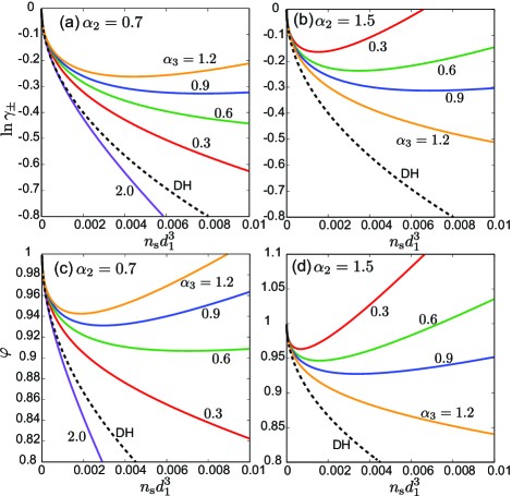
Figure 10: (Color online) $\ln\gamma_{\pm}$ and $\varphi$ in Eqs.(64)-(66) as functions of $n_{\rm s}d_{1}^{3}$ for $\alpha_{3}=0.3,0.6,0.9$, and $1.2$, where $\alpha_{2}$ is $0.7$ in (a) and (c) and is 1.5 in (b) and (d). The DH limiting curves are also shown (broken lines).

IV.6 Deviation constant $h$

Finally, we examine the deviation constant $h$ in the apparent partial volume $v_{\rm s}^{\rm ap}$ in Eq.(59)Desnoyers et al. (1969); Conway et al. (1966); Millero (1971, 1970). Experimentally, the ion-size-dependence of $h$ is opposite to that of $\ln\gamma_{\pm}$ and $\varphi$, as shown in Table IV. (i) We first consider alkali halidesDesnoyers et al. (1969). For ${F}^{-}$, $h$ decreases as the cation size increases. For the other anions, it exhibits the reverse dependence on the cation size. On the other hand, for cations of not large size (Li⁺, Na⁺, and K⁺), $h$ decreases as the anion size increases. For large Rb⁺ and Cs⁺, $h$ behaves non-monotonically. (ii) Second, for tetraalkylammonium Et₄N⁺ halidesConway et al. (1966), $h$ is negative and increases with increasing the anion size.

In our scheme, the unique behavior of $h$ arises if $\partial{\tilde{V}}_{\rm eff}/\partial p$ exceeds $\kappa_{\rm w}{\tilde{V}}_{\rm eff}$ in Eq.(60). In particular, $v_{i}^{\rm B}$ depends on $n_{1}$, so we consider the ratio $A_{\rm B}=n_{1}(\partial v_{i}^{\rm B}/\partial n_{1})/v_{i}^{\rm B}$. From Eq.(70) it is expressed as

$$A_{\rm B}=(\partial^{2}\epsilon/\partial p^{2})/(\epsilon\kappa_{\rm w}^{2}a_{\epsilon})-2a_{\epsilon},$$ (101)

where $a_{\epsilon}=n_{1}\epsilon^{\prime}/\epsilon=1.1$ in Eq.(17) and $R_{i}$ is assumed to be independent of $n_{1}$. Here, data of $\epsilon$ in ambient waterArcher and Wang (1990); Fern$\acute{\rm a}$ndez et al. (1997) give $(\partial^{2}\epsilon/\partial p^{2})_{T}\sim-6\times 10^{-7}/$MPa². Thus, we estimate $A_{\rm B}\sim-5$.

In Fig.11, we plot $h$ and $\partial{\tilde{U}}_{\rm eff}/\partial p$ vs $\alpha_{2}$ for various $\alpha_{3}$ setting $A_{\rm B}=-7.5$, where $\partial{\tilde{U}}_{\rm eff}/\partial p$ determines the overall behavior of $h$. The resultant $h$ behaves in the same manner as in the the experimentDesnoyers et al. (1969). Here, the two terms in Eq.(60) compete delicately depending on the parameter values. Indeed, if we set $A_{\rm B}=-5.0$ with the other parameters unchanged, the curves of $\alpha_{3}=0.7,0.9,$ and 1.1 increase with increasing $\alpha_{2}$ for $\alpha_{2}\gtrsim 0.8$. We also set $n_{1}\partial\ln\kappa_{\rm w}/\partial n_{1}=-8.3$, from Eqs.(80) and (81), though it is $-5.4$ in real waterFine and Millero (1973). Thus, to calculate $h$, we need to make very crude approximationsRedlich and Meyer (1964).

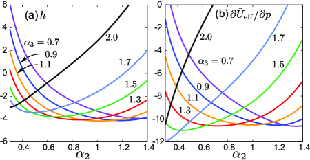
Figure 11: (Color online) (a) Deviation constant $h$ in Eq.(60) and (b) $\partial{\tilde{U}}_{\rm eff}/\partial p$ (the second term in Eq.(60)) vs $\alpha_{2}$ in units of $d_{1}^{6}$, where $\alpha_{3}=0.7,0.9,1.1,1.3,1.5,1.7$, and 2.0 from above.

Table 4: Data of $h$ for alkali halidesDesnoyers et al. (1969) and Et₄N⁺ halidesConway et al. (1966) in units of $\mathrm{cm}^{3}\mathrm{L}/\mathrm{mol}^{2}$ and in units of $d_{1}^{6}$ in the parentheses $()$. Here, 1 $\mathrm{cm}^{3}\mathrm{L}/\mathrm{mol}^{2}$ corresponds to $3.82d_{1}^{6}$ with $d_{1}=3$Å. Ion volume of Et₄N⁺ is $v_{2}^{*}\sim 9d_{1}^{3}$ $\sim 8n_{\rm w}^{-1}$.

	$\mathrm{F}^{-}$	$\mathrm{Cl}^{-}$	$\mathrm{Br}^{-}$	$\mathrm{I}^{-}$
$\mathrm{Li}^{+}$	1.1 (4.2)	-0.36 (-1.4)	-0.60 (-2.3)
$\mathrm{Na}^{+}$	0.64 (2.4)	-0.03 (-0.11)	-0.26 (-0.99)	-0.38 (-1.5)
$\mathrm{K}^{+}$	0.52 (2.0)	0.10 (0.38)	-0.16 (-0.61)	-0.39 (-1.5)
$\mathrm{Rb}^{+}$	0.55 (2.1)	0.17 (0.65)	-0.26 (-0.99)	-0.05 (-0.19)
$\mathrm{Cs}^{+}$	0.25 (0.95)	0.12 (0.46)	0.09 (0.34)	0.11 (0.42)
$\mathrm{Et}_{4}\mathrm{N}^{+}$		-21.0 (-80)	-19.4 (-74)	-6.0 (23)

V Summary and Remarks

In summary, we have presented a theory of electrolytes accounting for the deviation of the solvent density $\delta n_{1}$ induced by those of the ions. It has been neglected in the previous primitive theories. In Sec.III, we have then derived the ion volume $v_{i}^{*}$ in Eq.(19) and the effective ion-ion interaction coefficients $U_{ij}^{\rm eff}$ in Eq.(24) ($i,j=2,3)$. In the latter, the second bilinear term ($-v_{i}^{*}v_{j}^{*}/\kappa_{\rm w}$) arises from the solvent-mediated interactions and can explain Collins’ ruleCollins (1997) in the presence of the electrostriction (which leads to $v_{i}^{*}<0$ for small ions). Namely, it yields cation-anion repulsion for small-large ion pairs with $v_{i}^{*}v_{j}^{*}<0$ and attraction for symmetric pairs with $v_{i}^{*}v_{j}^{*}>0$. In the thermodynamic quantities, the mean interaction coefficient $U_{\rm eff}=\sum_{i,j=2,3}U_{ij}^{\rm eff}/2$ appears.

We have defined a parameter $\chi$ in the ionic fluctuation variances for $n_{2}$ and $n_{3}$ in Eq.(28) and expressed the Kirkwood-Buff integrals for $n_{1}$ and $n_{2}+n_{3}$ in terms of $\chi$ in Eqs.(36) and (37). We have expanded this $\chi$, the mean activity coefficient $\gamma_{\pm}$, the osmotic coefficient $\varphi$, and the apparent partial volume $v_{i}^{\rm ap}$ in powers of $\sqrt{n_{\rm s}}$ for small average salt density $n_{\rm s}=\langle{n_{2}}\rangle=\langle{n_{3}}\rangle$. In these expressions the first correction are the DH contributions.

We have also confirmed unique behavior of small-large ion pairs as predicted by Collins, where $U_{\rm eff}<0$ and $U_{23}^{\rm eff}>0$. As an extreme example, NaBPh₄ is strongly coupled with the water density with a largely negative $U_{\rm eff}$. For such a salt, we have discussed a spinodal instability for $n_{\rm s}$ exceeding $n_{\rm s}^{\rm spi}$ in Eq.(68)Okamoto and Onuki (2018).

In Sec.IV, we have performed numerical analysis using the Mansoori-Carnahan-Starling-Leland (MCSL) modelMansoori et al. (1971), the Lennard-Jones (LJ) attraction, and the Born model. We have calculated the ion volume $v_{i}^{*}$ and the excess coefficients $V_{ij}^{\rm eff}=U_{ij}^{\rm eff}-u_{ij}^{\rm ex}$ in Eq.(91) in Fig.7, where $u_{ij}^{\rm ex}$ are the contribution from the DH free energy in Eq.(6). Some asymptotic expressions have been given for them in Eqs.(90), (93), and (94). Regarding the ion-specific thermodynamic behavior, the mean interaction coefficient $U_{\rm eff}=\sum_{i,j=2,3}U_{ij}^{\rm eff}/2$ is a key quantity (see Eqs.(56)-(62))

We have found that the two steric parts in $U_{ij}^{\rm eff}$ in Eq.(24) or $V_{ij}^{\rm eff}$ in Eq.(91) mostly cancel, as calculated in Appendix E. Due to this cancellation, the effective interaction coefficients for purely steric hardsphere systems, $U_{hij}^{\rm eff}$ in Eq.(92), are not large as in Fig.4 and become smaller than the other contributions for ambient water, leading to Eqs.(93) and (94). Note that our hardcore quantities, $\nu_{i}^{h}$ and $U_{ij}^{h}$ in Eq.(74) and $1/\epsilon_{\rm in}^{h}$ in Eq.(81), are enlarged by the powers of $(1-\eta_{1})^{-1}$ for large solvent volume fraction $\eta_{1}(\sim 0.5$ for ambient water). In contrast, in the primitive modelsRasaiah and Friedman (1968); Waisman and Lebowitz (1970); Ebeling and Grigo (1982); Blum (1975); Simonin et al. (1996), the total packing fraction arises from the ions only and $U(=-k_{B}T\sum_{i,j}\int d{\mbox{\boldmath$r$}}c_{ij}^{0}(r)/2$) is positive and not very large (see Eq.(22)), so its expression (without the second term in Eq.(25)) was fitted to data of salts.

We have examined the Born part in $V_{ij}^{\rm eff}$, which yields singular interaction for small-large ion pairs. The remaining part consists of the MCSL and LJ contributions exhibiting rather simple behaviors in Fig.8. We have then presented simple interpolation formulas for $V_{ij}^{\rm eff}$ in Eqs.(97)-(99). We have calculated $\chi^{-1}$, $w_{\rho}$, $\ln\gamma_{\pm}$, and $\varphi$ as functions of $\alpha_{2}$, $\alpha_{3}$, and $n_{\rm s}$ in Figs.9 and 10. We have also examined the deviation constant $h$ in $v_{\rm s}^{\rm ap}$ in Fig.11, which behaves differently from the others.

We make some remarks.
(i) Our numerical analysis is very approximate. In particular, the parameter choices in Eqs.(83)-(86) remain still arbitrary, where the specific properties of cations and anions are neglected. Nevertheless, our theory provides simple, overall understanding of the puzzling behaviors of electrolytes. The results in Fig.7 should be commonly expected for various solvents (see Appendix F). (ii) We should calculate the structure factors of water and ions at finite wave numbers including the DH interaction and the effective mutual interactions. (iii) It is informative to perform molecular dynamics simulations for various ion pairs, for example, to confirm the behaviors in Fig.7 and Eqs.(97)-(99). (iv) We have mentioned singular behaviors of small-large ion pairs in waterCollins (1997), which include antagonistic saltsOnuki et al. (2016) such as NaBPh₄. It is of great interest to perform scattering experimentsCollins et al. (2007) for salts with small or negative $\chi^{-1}$. (v) In mixture solvents such as water-alcohol, the solvent-mediated interaction is much enhanced due to the concentration fluctuationsOkamoto and Onuki (2018). Thus, we need to study electrolytes of mixture solvents.

AIP Publishing Data Sharing Policy
The data that support the findings of this study are avail- able from the corresponding author upon reasonable re- quest.

Appendix A: Bjerrum dipoles

Here, we examine how the Bjerrum dipoles alter our theory. For nonvanishing dipole density $n_{\rm d}$, we change the free energy density $f$ in Eq.(2) toZwanikken and van Roij (2009)

$${\tilde{f}}=f+k_{B}Tn_{\rm d}[\ln(n_{\rm d}\lambda_{\rm d}^{3})-1-\nu_{\rm d}+2\nu],$$ (A1)

where $k_{B}T\nu_{\rm d}$ is the free energy decrease due to the association per dipole and $\nu$ is defined by Eq.(8). If we neglect inhomogeneous density deviations, we have $n_{2}=n_{3}=n_{\rm s}-n_{\rm d}$, where $n_{\rm s}$ is the added salt density (held fixed here). In equilibrium, the dipole chemical potential $\mu_{\rm d}=\partial{\tilde{f}}/\partial n_{\rm d}$ equals $\mu_{\rm s}$ in Eq.(41); then,

$${n_{\rm d}}=Kn_{\rm s}^{2}+\cdots,\quad{n_{2}}={n_{3}}=n_{\rm s}-Kn_{\rm s}^{2}+\cdots.$$ (A2)

where $n_{\rm s}\ll K^{-1}$ with $K$ being the association constant,

$$K=(\lambda^{6}/\lambda_{\rm d}^{3})\exp({\nu_{\rm d}}).$$ (A3)

If $n_{\rm d}$ is removed, the free energy density is lowered as

$${\tilde{f}}(n_{1},n_{2},n_{3},n_{\rm d})={f}(n_{\rm w},n_{\rm s},n_{\rm s})-k_{B}TKn_{\rm s}^{2}+\cdots,$$ (A4)

where the logarithmic term $k_{B}Tn_{\rm d}\ln(n_{\rm d}\lambda_{\rm d}^{3})$ disappears. Thus, if we accept Bjerrum’s assumption, $U_{23}$ in Eq.(3) is changed to $U_{23}-k_{B}TK$. Then, $\ln\gamma_{\pm}$ decreases by $Kn_{\rm s}$.

Appendix B: Gibbs free energy of electrolytes

We calculate the Gibbs free energy $G$. As in Sec.IIID, we fix $p$, $T$, and the total solvent number $N_{\rm w}=Vn_{\rm w}=V_{0}n_{\rm w}^{0}$. Here, without salt at pressure $p$, the solvent density is $n_{\rm w}^{0}$ and the volume is $V_{0}$.

We integrate $dG/dN_{\rm s}=\mu_{\rm s}$ with respect to $N_{\rm s}$ using Eq.(41), where we set $n_{\rm s}=N_{\rm s}/V\cong(N_{\rm s}/V_{0})(1-{\bar{v}}_{{\rm s}}^{0}N_{\rm s}/V_{0})$ in $\ln(n_{\rm s}\lambda^{3})$. Up to order $n_{\rm s}^{2}$, we obtainRobinson and Stokes (2002); Pitzer (1973)

$$G=N_{\rm w}\mu_{\rm w}^{0}(n_{\rm w}^{0})+2k_{B}TN_{\rm s}[\ln(\lambda^{3}N_{\rm s}/V_{0})-1+\nu(n_{\rm w}^{0})]$$

$$\hskip 8.53581pt+V_{0}(-k_{B}T\kappa^{3}/12+{\tilde{U}}_{\rm eff}n_{\rm s}^{2}),$$ (B1)

where $\mu_{\rm w}^{0}(n_{\rm w}^{0})$ is the chemical potential of pure solvent at the density $n_{\rm w}^{0}$ and ${\tilde{U}}_{\rm eff}$ is given in Eq.(57).

Since $n_{\rm w}^{0}$ is determined by $p$ and $T$, we can treat $G$ in Eq.(B1) as a function of $N_{\rm w}$, $N_{\rm s}$, $p$, and $T$. Then,

$$V=(\partial G/\partial p)_{N_{\rm w},N_{\rm s},T}=V_{0}+v_{\rm s}^{\rm ap}N_{\rm s},$$ (B2)

from which we can calculate the apparent partial volume $v_{\rm s}^{\rm ap}$ to derive Eqs.(59) and (60) up order $n_{\rm s}^{2}$. The partial volume ${\bar{v}}_{\rm s}$ in Eq.(46) can be related to $v_{\rm s}^{\rm ap}$ as

$${\bar{v}}_{\rm s}=[v_{\rm s}^{p}+n_{\rm s}(\partial v_{\rm s}^{p}/\partial n_{\rm s})]/[1+n_{\rm s}^{2}(\partial v_{\rm s}^{p}/\partial n_{\rm s})],$$ (B3)

where $\partial v_{\rm s}^{p}/\partial n_{\rm s}$ is the derivative at fixed $p$ and $T$. On the other hand, from $G=N_{\rm w}\mu_{\rm w}+N_{\rm s}\mu_{\rm s}$, the osmotic coefficient $\varphi$ in Eq.(61) is expressed as

$$\varphi=[N_{\rm w}\mu_{\rm w}^{0}(n_{\rm w}^{0})+N_{\rm s}\mu_{\rm s}-G]/(2k_{B}TN_{\rm s}),$$ (B4)

leading to Eq.(62) with the aid of Eqs.(41) and (B1).

Appendix C:Derivation of Eqs.(50) and (59)

We rewrite Eqs.(49) and (58) as

$$dn_{\rm w}/dn_{\rm s}=b_{1}(n_{\rm w})+b_{2}(n_{\rm w})n_{\rm s}^{1/2}+b_{3}(n_{\rm w})n_{\rm s}+\cdots,$$ (C1)

where $b_{1}$, $b_{2}$, and $b_{3}$ are functions of $n_{\rm w}$. Up to order $n_{\rm s}^{2}$, Eq.(C1) yields the deviation $\delta n_{\rm w}=n_{\rm w}(n_{\rm s})-n_{\rm w}^{0}$ as

$$\delta n_{\rm w}=b_{1}(n_{\rm w})n_{\rm s}+\frac{2}{3}b_{2}(n_{\rm w})n_{\rm s}^{3/2}+\frac{1}{2}c_{3}(n_{\rm w})n_{\rm s}^{2}+\cdots$$

$$=b_{1}(n_{\rm w}^{0})n_{\rm s}+\frac{2}{3}b_{2}(n_{\rm w}^{0})n_{\rm s}^{3/2}+\frac{1}{2}{\tilde{c}}_{3}(n_{\rm w}^{0})n_{\rm s}^{2}+\cdots,$$ (C2)

where the second line is written in terms of $n_{\rm w}^{0}$ as in Eqs.(50) and (59). Thus, $b_{1}(n_{\rm w})\cong b_{1}(n_{\rm w}^{0})+b_{1}^{\prime}\delta n_{\rm w}$, where $b_{1}^{\prime}=db_{1}/dn_{\rm w}$. We differentiate the first line of Eq.(C2) with respect to $n_{\rm s}$ to find

$$c_{3}=b_{3}-b_{1}b_{1}^{\prime},\quad{\tilde{c}}_{3}=b_{3}+b_{1}b_{1}^{\prime}.$$ (C3)

The expression for ${\tilde{c}}_{3}$ leads to Eqs.(50) and (59).

Appendix D: Extended expressions of $\chi^{-1}$ and $v_{\rm s}^{\rm ap}$

We rewrite $\chi^{-1}$ in Eq.(32) and $v_{\rm s}^{\rm ap}$ in Eq.(59) as

$$\chi^{-1}=2-\frac{1}{4}\ell_{B}\kappa\sum_{i=2,3}\frac{1}{(1+a_{i}\kappa)^{2}}+\frac{2n_{\rm s}}{k_{B}T}V_{\rm eff},$$ (D1)

$${v}_{\rm s}^{\rm ap}={\bar{v}}_{{\rm s}}^{0}(n_{\rm w}^{0})+{\epsilon_{\rm in}{\ell}_{B}\kappa}\sum_{i=2,3}\Big{[}\frac{\epsilon^{\prime}/2\epsilon}{1+a_{i}\kappa}-\frac{\sigma(a_{i}\kappa)}{6n_{\rm w}}\Big{]}$$

$$\hskip 11.38109pt+[\kappa_{\rm w}{\tilde{V}}_{\rm eff}+\partial{\tilde{V}}_{\rm eff}/\partial p]n_{\rm s}.$$ (D2)

We define $V_{\rm eff}$ in Eq.(91) and ${\tilde{V}}_{\rm eff}$ in Eq.(57). In Eq.(D2), the first term is ${\bar{v}}_{{\rm s}}^{0}$ at the initial density $n_{\rm w}^{0}$ and $\sigma(x)$ is defined below Eq.(65). These expressions tend to Eqs.(32) and (59) as $a_{i}\kappa\to 0$.

Appendix E: MCSL model of hardsphere fluids

Here, we summarize the MCSL model of hardsphere fluid mixtures of $m$ componentsMansoori et al. (1971), where $m=3$ in this paper. Setting $n=\sum_{i}n_{i}$, $\eta_{i}={\pi}n_{i}d_{i}^{3}/6$, $\eta=\sum_{j}\eta_{j}$, and $u=\eta/(1-\eta)$, we write $f_{h}(n_{1},n_{2},n_{3})$ in Eq.(73) as^,Zhang et al. (2016)

$$\frac{f_{h}}{k_{B}Tn}=4u+u^{2}-3y_{1}u+(y_{3}-1)[u+{u^{2}}+\ln(1-\eta)].$$ (E1)

Setting $\sigma_{\ell}=\sum_{i}\pi d_{i}^{\ell}n_{i}/6$, we define $y_{1}$ and $y_{3}$ as

$$y_{1}=1-6\sigma_{1}\sigma_{2}/(\pi n\eta),~{}~{}y_{3}={6\sigma_{2}^{3}}/({{\pi\eta^{2}n}}),$$ (E2)

where $y_{1}\to 0$ and $y_{3}\to 1$ in the one-component limit.

From Eq.(E1) we obtain the MCSL chemical potentials $\partial f_{h}/\partial n_{i}$. In the dilute case, $\nu_{i}^{h}$ in Eq.(74) are written as

$$\nu_{i}^{\rm h}= (3\alpha_{i}+6\alpha_{i}^{2}-\alpha_{i}^{3})u_{1}+(3\alpha_{i}^{2}+4\alpha_{i}^{3})u_{1}^{2}$$

$$+2\alpha_{i}^{3}u_{1}^{3}+(3\alpha_{i}^{2}-2\alpha_{i}^{3}-1)\ln(1-\eta_{1}),$$ (E3)

where $u_{1}=\eta_{1}/(1-\eta_{1})$. The right hand side steeply grows with increasing $\eta_{1}$ (see Fig.3 in our previous paperOkamoto and Onuki (2016)). The MCSL ion volume $v_{i}^{h}=\epsilon_{\rm in}{d}\nu_{i}^{h}/{dn_{1}}$ is given by

$${v_{i}^{h}}=(w_{\rm a}+1-\epsilon_{\rm in}u_{1}^{2})\alpha_{i}^{3}v_{1}+\epsilon_{\rm in}\psi_{i}v_{1},$$ (E4)

where $v_{1}=\pi d_{1}^{3}/6$ and $w_{\rm a}$ is defined in Eq.(82). Setting $x_{1}=1/(1-\eta_{1})$, we define $\psi_{i}$ by

$$\psi_{i}={6\alpha_{i}^{2}}x_{1}^{3}+{3\alpha_{i}}x_{1}^{2}+({1-3\alpha_{i}^{2}})x_{1}.$$ (E5)

For $\alpha_{i}=1$, we simply find $v_{i}^{h}=n_{1}^{-1}(1+w_{\rm a}-\epsilon_{\rm in}).$ For considerably large $\alpha_{i}$ (say, $\alpha_{i}\sim 1.4$), the second term in Eq.(E4) is of order $v_{1}$, but it is considerably cancelled by negative $v_{i}^{\rm LJ}$ (see Fig.3). We thus find Eq.(89).

From Eqs.(E1) and (74) we express $U_{ij}^{h}$ as

$${U_{ij}^{h}}/{v_{1}k_{B}T}=\alpha_{i}^{3}\alpha_{j}^{3}\Phi_{1}+\alpha_{ij}^{2}(\alpha_{ij}+3\alpha_{i}\alpha_{j}u_{1})/(1-\eta_{1})$$

$$+6\alpha_{i}^{2}\alpha_{j}^{2}\Big{[}(\alpha_{ij}-1)\Big{(}u_{1}^{3}+2u_{1}^{2}+\zeta_{1}\Big{)}+u_{1}/(1-\eta_{1})^{2}\Big{]},$$ (E6)

where $\alpha_{ij}=\alpha_{i}+\alpha_{j}$ and $\zeta_{1}=-1-\eta_{1}^{-1}\ln(1-\eta_{1})$. Using $\psi_{i}$ we also express $U_{hij}^{\rm eff}$ in Eq.(92) as

$${U_{hij}^{\rm eff}}/{v_{1}k_{B}T}=\alpha_{i}^{3}\alpha_{j}^{3}\Phi_{2}+3\alpha_{i}^{2}\alpha_{j}^{2}(\alpha_{ij}-1)(2\zeta_{1}-{u_{1}})$$

$$+3\alpha_{i}^{2}\alpha_{j}^{2}(3-\eta_{1})u_{1}/(1-\eta_{1})+\alpha_{ij}^{3}+3\alpha_{ij}\alpha_{i}\alpha_{j}u_{1}$$

$$+\epsilon_{\rm in}^{h}\eta_{1}[(\psi_{i}\alpha_{j}^{3}+\psi_{j}\alpha_{i}^{3})u_{1}^{2}-\psi_{i}\psi_{j}].$$ (E7)

As the coefficients of $\alpha_{i}^{3}\alpha_{j}^{3}$, we define $\Phi_{1}$ and $\Phi_{2}$ as

$$\Phi_{1} = \Phi_{2}+\eta_{1}(1-u_{1}^{2}\epsilon_{\rm in}^{h})^{2}/\epsilon_{\rm in}^{h},$$ (E8)

$$\Phi_{2} = {2\eta_{1}}/{(1-\eta_{1})}+\eta_{1}-6\zeta_{1}-\epsilon_{\rm in}^{h}\eta_{1}u_{1}^{4},$$ (E9)

where $\Phi$ is large ($\gg 1$) but $\Phi_{2}$ is small ($\ll 1$) for $\eta_{1}\sim 0.5$. In fact, $\Phi_{2}\cong\eta_{1}^{3}/2$ for $\eta_{1}\ll 1$ and $\Phi_{2}\sim 0.1$ for $\eta_{1}\sim 0.5$. Thus, the first term in Eq.(E7) is negligible for not very large $\alpha_{i}\alpha_{j}$. For small $\alpha_{i}$ and $\alpha_{j}$ ($\ll 1)$, we have ${U_{hij}^{\rm eff}}/v_{1}k_{B}T\cong-\epsilon_{\rm in}\eta_{1}/(1-\eta_{1})^{2}$. We plot ${U_{hij}^{\rm eff}}$ in Fig.4.

Now, we rewrite $V_{ij}^{\rm eff}$ in Eq.(91) as

$$V_{ij}^{\rm eff}={U_{hij}^{\rm eff}}-w_{ij}-(v_{i}^{*}v_{j}^{*}-v_{i}^{h}v_{j}^{h}\epsilon_{\rm in}^{h}/\epsilon_{\rm in})/\kappa_{\rm w},$$ (E10)

where the MCSL contribution is subtracted in the third term. Here, the third term dominates over the first with significant attractive and hydration interactions. The above expression leads to Eqs.(93) and (94).

Appendix F: Marginal ion-size-dependence

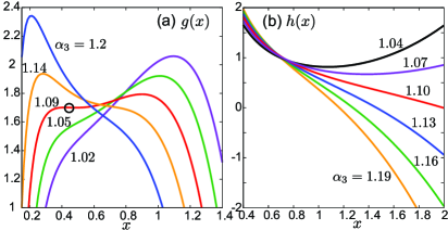
Figure 12: (Color online) (a) $g(x)=V_{\rm eff}/(k_{B}Td_{1}^{3}B\alpha_{3}^{2})$ in Eq.(F1) vs $x=\alpha_{2}/\alpha_{3}$ at fixed $\alpha_{3}$. Line of $\alpha_{3}=1.09$ has an inflection point ($\circ$). (b) $h(x)=V^{\rm eff}_{23}/(k_{B}Td_{1}^{3}B\alpha_{3}^{2})$ in Eq.(F6). These functions are nearly flat for $\alpha_{3}\cong 1.1$.

We first show the existence of an inflection point in $V_{\rm eff}$ vs $\alpha_{2}$, where $\partial V_{\rm eff}/\partial\alpha_{2}=\partial^{2}V_{\rm eff}/\partial\alpha_{2}^{2}=0$ at a certain $\alpha_{3}$. Using Eq.(97), we define $g(x)=V_{\rm eff}/(k_{B}Td_{1}^{3}B\alpha_{3}^{2})$. As a function of $x=\alpha_{2}/\alpha_{3}$ at fixed $\alpha_{3}$, $g(x)$ is expressed as

$$g(x)=(1+\frac{1}{x})\Big{[}(1+x^{3})-\frac{C^{\prime}}{2}(1+\frac{1}{x})\Big{]}-\frac{A^{\prime}}{2}(1+x^{3})^{2},$$ (F1)

where $C^{\prime}=C/B\alpha_{3}^{4}=D_{\rm B}/(D_{\rm L}\alpha_{3}^{4})$ and $A^{\prime}=A\alpha_{3}^{4}/B$ with $A=5.0$, $B=7.0$, and $C=2.8$ (see below Eq.(97)), so we fix $A^{\prime}C^{\prime}=0.29$. We require $dg/dx=d^{2}g/dx^{2}=0$ at the inflection point to obtain

$$3x^{4}-x^{3}+x^{2}-x+C^{\prime}=3A^{\prime}x^{5}(x^{2}-x+1),$$ (F2)

$$12x^{3}-3x^{2}+2x-1=3A^{\prime}x^{4}(7x^{2}-6x+5),$$ (F3)

The critical values of $x$ and $C^{\prime}$ are $x_{c}=0.45$ and $C_{c}^{\prime}=0.25$, respectively. The critical value of $\alpha_{3}$ is given by

$$\alpha_{3c}=(D_{\rm B}/D_{\rm L}C_{c}^{\prime})^{1/4}=1.09.$$ (F4)

which is close to 1 owing to the small exponent $1/4$. However, $x_{c}$ is considerably smaller than 1, so the right hand sides of Eqs.(F2) and (F3) are negligible near the inflection point. For small $\alpha_{3}-\alpha_{3c}$ and $x-x_{c}$, we find

$$g(x)\cong 7(x-x_{c})^{3}-16(\alpha_{3}-\alpha_{3c})(x-x_{c})+1.7.$$ (F5)

Thus, the slope of $g(x)$ vs $x$ changes its sign abruptly for $\alpha_{3}\cong\alpha_{3c}$ as in Fig.7(a), which is analogous to the isothermal pressure-density relation in the van der Waals equation of state.

Table 5: Values of $\epsilon$, $\ell_{B}$ ($\rm\AA$), $(\partial\ln\epsilon/\partial p)_{T}$ (GPa^-1), $d_{1}$ ($\rm\AA$), $\beta_{1}$, and $\alpha_{3{\rm c}}$ for six solvents at $T=300$ K.

	$\epsilon$	$\ell_{B}$	$\partial\ln\epsilon/\partial p$	$d_{1}$	$\beta_{1}$	$\alpha_{3{\rm c}}$
water	80	7	0.47	3	0.91	1.09
formamide	111	5	0.45	3.9	0.62	0.74
methanol	33	17	1.2	3.9	1.09	1.31
ethanol	25	22	1.2	4.4	1.03	1.24
acetonitrile	37	15	1.1	4.3	0.96	1.15
acetone	21	27	1.6	4.8	1.07	1.28

Second, we consider the normalized cation-anion interaction coefficient $h(x)=V_{23}^{\rm eff}/(k_{B}Td_{1}^{3}B\alpha_{3}^{2})$. From Eq.(99), $h(x)$ depends on $x=\alpha_{2}/\alpha_{3}$ as

$$h(x)=(1-A^{\prime})x^{3}+(1-C^{\prime})/x,$$ (F6)

which has no inflection point. However, if $A^{\prime}\cong 1$ or $\alpha_{3}\cong(B/A)^{1/4}\sim 1.1$, $h(x)$ is nearly flat, say, in the range $[0.6,1.2]$ as in Fig. 12(b). For example, we have $A^{\prime}=1.05$ and 0.94 for $\alpha_{3}=1.10$ and 1.07, respectively. This behavior can be seen in Fig.7(b).

Third, we discuss the marginal size-dependence of $V_{\rm eff}$ for nonaqueous solvents. From Eq.(F4) and the sentences below Eq.(90), we have $\alpha_{3{\rm c}}=\beta_{1}\beta_{2}$ with

$$\beta_{1}=[4\ell_{B}\epsilon_{\rm in}\epsilon^{\prime}/\epsilon]^{1/4}/d_{1},\quad\beta_{2}=(d_{i}/2R_{i}D_{\rm L})^{1/4},$$ (F7)

where we set $C_{c}^{\prime}=1/4$. We also set $\beta_{2}=1.2$ as in the case of water, while $\beta_{1}$ depends on the solvent species. For nonaqueous solvents, we assume $d_{1}=n_{1}^{-1/3}$ and use published experimental data at $T\sim 300$K and $p\sim 1$ atmMazzinia and Craig (2017); Marcus and Hefter (1999). We then obtain Table V, where $\alpha_{3{\rm c}}\sim 1$ for all the solvents (again largely due to the exponent $1/4$).

References

- Robinson and Stokes (2002) R. A. Robinson and R. H. Stokes, Electrolyte Solutions, 2nd ed. (Dover: Mineola, NY, 2002).
- Hamann et al. (2007) C. H. Hamann, A. Hamnett, and W. Vielstich, Electrochemistry (Wiley-VCH, 2007).
- Debye and Hückel (1923) P. Debye and E. Hückel, Phys. Z. 24, 185 (1923).
- McQuarrie (1976) D. McQuarrie, Statistical Mechanics, Chap.15 (Harper and Row, New York, 1976).
- Kunz et al. (2004a) W. Kunz, P. L. Nostro, and B. W. Ninham, Curr. Opin. Coll. Int. Sci. 9, 1 (2004a).
- Kunz (2010) W. Kunz, Curr. Opin. Coll. Int. Sci. 15, 34 (2010).
- Nostro and Ninham (2012) P. L. Nostro and B. W. Ninham, Chem. Rev. 112, 2286 (2012).
- Kunz et al. (2004b) W. Kunz, J. Henle, and B. W. Ninham, Curr. Opin. Coll. Int. Sci. 9, 19 (2004b).
- Hückel (1925) E. Hückel, Z. Phys. 28, 93 (1925).
- Born (1920) M. Born, Z. Physik 1, 45 (1920).
- Millero (1971) F. J. Millero, Chem. Rev. 71, 147 (1971).
- Marcus (2011) Y. Marcus, Chem. Rev. 111, 2761 (2011).
- Lewis and Randall (1921) G. N. Lewis and M. Randall, J. Am. Chem. Soc. 43, 1112 (1921).
- Brnsted (1922) J. N. Brnsted, J. Am. Chem. Soc. 44, 938 (1922).
- Guggenheim (1935) E. A. Guggenheim, Phi. Mag. 19, 588 (1935).
- Guggenheim and Turgen (1955) E. A. Guggenheim and J. Turgen, Trans. Faraday Soc. 51, 747 (1955).
- Bromley (1973) L. A. Bromley, AIChE J. 19, 313 (1973).
- Pitzer (1973) K. S. Pitzer, J. Phys. Chem. 77, 268 (1973).
- Pailthorpe et al. (1984) B. A. Pailthorpe, D. J. Mitchell, and B. W. Ninham, J. Chem. Soc., Faraday Trans. 2 80, 115 (1984).
- Redlich (1940) O. Redlich, J. Phys. Chem. 44, 619 (1940).
- Redlich and Meyer (1964) O. Redlich and D. M. Meyer, Chem. Rev. 64, 221 (1964).
- Conway et al. (1966) B. E. Conway, R. . E. Verrall, and J. E. Desnyers, Trans. Faraday Soc. 62, 2738 (1966).
- Desnoyers et al. (1969) J. E. Desnoyers, M. Arel, G. Perron, and C. Jolicoeur, J. Phys. Chem. 73, 3346 (1969).
- Rasaiah and Friedman (1968) J. C. Rasaiah and H. L. Friedman, J. Chem. Phys. 48, 2742 (1968).
- Waisman and Lebowitz (1970) E. Waisman and J. L. Lebowitz, J. Chem. Phys. 52, 4307 (1970).
- Blum (1975) L. Blum, Mol. Phys. 30, 1529 (1975).
- Simonin et al. (1996) J. P. Simonin, L. Blum, and P. Turq, J. Phys. Chem. 100, 7704 (1996).
- Ebeling and Grigo (1982) W. Ebeling and M. Grigo, J. Solution Chem. 11, 151 (1982).
- Levin and Fisher (1996) Y. Levin and M. E. Fisher, Physica A 225, 164 (1996).
- Stell (1996) G. Stell, J. Stat. Phys. 78, 197 (1996).
- Card and Valleau (1970) D. N. Card and J. P. Valleau, J. Chem. Phys. 52, 6232 (1970).
- Romero-Enrique et al. (2000) J. M. Romero-Enrique, G. Orkoulas, A. Z. Panagiotopoulos, and M. E. Fisher, Phys. Rev. Lett. 85, 4558 (2000).
- Ramanathan and Friedman (1971) P. S. Ramanathan and H. L. Friedman, J. Chem. Phys. 54, 1086 (1971).
- Blum (1974) L. Blum, J. Chem. Phys. 61, 2129 (1974).
- Perkyns and Pettitt (1992) J. Perkyns and B. M. Pettitt, J. Chem. Phys. 97, 7656 (1992).
- Kalyuzhnyi et al. (2010) Y. V. Kalyuzhnyi, V. Vlachy, and K. A. Dill, Phys. Chem. Chem. Phys. 12, 6260 (2010).
- Joung et al. (2013) I. S. Joung, T. Luchko, and D. A. Case, J. Chem. Phys. 138, 044103 (2013).
- Weerasinghe and Smith (2003) S. Weerasinghe and P. E. Smith, J. Chem. Phys. 119, 11342 (2003).
- Hess et al. (2006a) B. Hess, C. Holm, and N. van der Vegt, J. Chem. Phys. 124, 164509 (2006a).
- Hess et al. (2006b) B. Hess, C. Holm, and N. van der Vegt, Phys. Rev. Lett 96, 147801 (2006b).
- Kalcher and Dzubiella (2009) I. Kalcher and J. Dzubiella, J. Chem. Phys. 130, 134507 (2009).
- Vrbka et al. (2009) L. Vrbka, M. Lund, I. Kalcher, J. Dzubiella, R. R. Netz, and W. Kunz, J. Chem. Phys. 131, 154109 (2009).
- Klasczyk and Knecht (2010) B. Klasczyk and V. Knecht, J. Chem. Phys. 132, 024109 (2010).
- Fyta and Netz (2012) M. Fyta and R. R. Netz, J. Chem. Phys. 136, 124103 (2012).
- Kohns et al. (2016) M. Kohns, M. Schappals, M. Horsch, and H. Hasse, J. Chem. Eng. Data 61, 4068 (2016).
- Naleem et al. (2018) N. Naleem, N. Bentenitis, and P. E. Smith, J. Chem. Phys. 148, 222828 (2018).
- Kirkwood and Buff (1951) J. G. Kirkwood and F. P. Buff, J. Chem. Phys. 19, 774 (1951).
- Widom and Underwood (2012) B. Widom and R. C. Underwood, J. Phys. Chem. B 116, 9492 (2012).
- Koga et al. (2015) K. Koga, V. Holten, and B. Widom, J. Phys. Chem. B 119, 13391 (2015).
- Cerdeiria and Widom (2016) C. A. Cerdeiria and B. Widom, J. Phys. Chem. B 120, 13144 (2016).
- McMillan and Mayer (1945) W. G. McMillan and J. E. Mayer, J. Chem. Phys. 13, 276 (1945).
- Evans and Sluckin (1980) R. Evans and T. J. Sluckin, Mol. Phys. 40, 413 (1980).
- Onuki (2006) A. Onuki, Phys. Rev. E 73, 021506 (2006).
- Bazant et al. (2009) M. Z. Bazant, M. S. Kilic, B. D. Storey, and A. Ajdari, Adv. Coll. Int. Sci. 152, 48 (2009).
- Ben-Yaakov et al. (2011) D. Ben-Yaakov, D. Andelman, R. Podgornik, and D. Harries, Curr. Opin. Colloid Interface Sci. 16, 542 (2011).
- Fogolari et al. (2002) F. Fogolari, A. Brigo, and H. Molinari, J. Mol. Recognit. 15, 377 (2002).
- Bikerman (1942) J. J. Bikerman, Philos. Mag. 33, 384 (1942).
- Borukhov et al. (1997) I. Borukhov, D. Andelman, and H. Orland, Phys. Rev. Lett. 79, 435 (1997).
- Kralj-Igli and Igli (1996) V. Kralj-Igli and A. Igli, J. de Physique II 6, 477 (1996).
- Onuki (2002) A. Onuki, Phase Transition Dynamics (Cambridge, 2002).
- Mansoori et al. (1971) G. A. Mansoori, N. F. Carnahan, K. E. Starling, and T. W. Leland, J. Chem. Phys. 54, 1523 (1971).
- Biesheuvel and van Soestbergen (2007) P. M. Biesheuvel and M. van Soestbergen, J. Colloid Interface Sci. 316, 490 (2007).
- Zhang et al. (2016) P. Zhang, N. M. Alsaifi, J. Wu, and Z.-G. Wang, Macromolecules 49, 9720 (2016).
- Carnahan and Starling (1969) N. F. Carnahan and K. E. Starling, J. Chem. Phys. 51, 635 (1969).
- Okamoto and Onuki (2015) R. Okamoto and A. Onuki, Eur. Phys. J. E 38, 72 (2015).
- Okamoto and Onuki (2016) R. Okamoto and A. Onuki, J. Phys.: Condens. Matter 28, 244012 (2016).
- Okamoto and Onuki (2018) R. Okamoto and A. Onuki, J. Chem. Phys. 149, 014501 (2018).
- Kunz et al. (2016) W. Kunz, K. Holmberg, and T. Zemb, Curr. Opin. Colloid Interface Sci. 22, 99 (2016).
- Collins (1997) K. D. Collins, Biophys. J. 72, 65 (1997).
- Collins et al. (2007) K. D. Collins, G. W. Neilson, and J. E. Enderby, Biophysical Chemistry 128, 95 (2007).
- Collins (2019) K. D. Collins, Quarterly Reviews of Biophysics 52, e11 (2019).
- Schurhammer and Wipff (2000) R. Schurhammer and G. Wipff, J. Phys. Chem. A 104, 11159 (2000).
- Herrington and Taylor (1982) T. M. Herrington and C. M. Taylor, J. Chem. Soc., Faraday Trans. 1 78, 3409 (1982).
- Millero (1970) F. J. Millero, J. Chem. Eng. Data 15, 562 (1970).
- Sadakane et al. (2009) K. Sadakane, A. Onuki, K. Nishida, S. Koizumi, and H. Seto, Phys. Rev. Lett. 103, 167803 (2009).
- Onuki et al. (2016) A. Onuki, S. Yabunaka, T. Araki, and R. Okamoto, Curr. Opin. Coll. Int. Sci. 22, 59 (2016).
- Yabunaka and Onuki (2017) S. Yabunaka and A. Onuki, Phys. Rev. Lett. 119, 118001 (2017).
- Tasios et al. (2017) N. Tasios, S. Samin, R. van Roij, and M. Dijkstra, Phys. Rev. Lett. 119, 218001 (2017).
- Bjerrum (1926) N. Bjerrum, Kgl. Dan. Vidensk. Selsk. Mat.-Fys. Medd. 7, 1 (1926).
- Smith and Dang (1994) D. E. Smith and L. X. Dang, J. Chem. Phys. 100, 3757 (1994).
- Degrve and da Silva (1999) L. Degrve and F. L. B. da Silva, J. Chem. Phys. 110, 3070 (1999).
- Marcus and Hefter (2006) Y. Marcus and G. Hefter, Chem. Rev. 106, 4585 (2006).
- Hassan (2008) S. A. Hassan, J. Phys. Chem. B 112, 10573 (2008).
- Fennell et al. (2009) C. J. Fennell, A. Bizjak, V. Vlachy, and K. A. Dill, J. Phys. Chem. B 113, 6782 (2009).
- Zwanikken and van Roij (2009) J. Zwanikken and R. van Roij, J. Phys.: Condens. Matter 21, 424102 (2009).
- van der Vegt et al. (2016) N. F. A. van der Vegt, K. Haldrup, S. Roke, J. Zheng, M. Lund, and H. J. Bakker, Chem. Rev. 116, 7626 (2016).
- Adar et al. (2017) R. M. Adar, T. Markovich, and D. Andelman, J. Chem. Phys. 146, 194904 (2017).
- Note (1) In the original paperDebye and Hückel (1923), and can be different, while they have been equated in most subsequent papers.
- Archer and Wang (1990) D. G. Archer and P. Wang, J. Phys. Chem. Ref. Data 19, 371 (1990).
- Fernndez et al. (1997) D. P. Fernndez, A. R. H. Goodwin, E. W. Lemmon, J. M. H. L. Sengers, and R. C. Williams, J. Phys. Chem. Ref. Data 26, 1125 (1997).
- Hepler (1957) L. G. Hepler, J. Phys. Chem. 61, 1426 (1957).
- Mukerjee (1960) P. Mukerjee, J. Phys. Chem. 65, 740 (1960).
- Padova (1963) J. Padova, J. Chem. Phys. 39, 1552 (1963).
- Mazzinia and Craig (2017) V. Mazzinia and V. S. J. Craig, Chem. Sci. 8, 7052 (2017).
- O’Connell and DeGance (1975) J. P. O’Connell and A. E. DeGance, J. Solution Chem. 4, 763 (1975).
- Attard (1993) P. Attard, Phys. Rev. E 48, 3604 (1993).
- de Carvalho and Evans (1994) R. L. de Carvalho and R. Evans, Mol. Phys. 83, 619 (1994).
- Hansen and McDonald (1986) J. P. Hansen and I. R. McDonald, Theory of Simple Liquids (Academic, 1986).
- Chandler (2005) D. Chandler, Nature 437, 640 (2005).
- Lund et al. (2010) M. Lund, B. Jagoda-Cwiklik, C. E. Woodward, R. Vácha, and P. Jungwirth, Phys. Chem. Lett. 1, 300 (2010).
- Duignan et al. (2014) T. T. Duignan, D. F. Parsons, and B. W. Ninham, Phys. Chem. Chem. Phys. 16, 22014 (2014).
- Smith et al. (2016) A. M. Smith, A. A. Lee, and S. Perkin, J. Phys. Chem. Lett. 7, 2157 (2016).
- Adar et al. (2019) R. M. Adar, S. A. Safran, H. Diamant, and D. Andelman, Phys. Rev. E 100, 042615 (2019).
- Coles et al. (2020) S. W. Coles, C. Park, R. Nikam, M. Kandu, J. Dzubiella, and B. Rotenberg, J. Phys. Chem. B 124, 1778 (2020).
- Kusalik and Patey (1987) P. G. Kusalik and G. N. Patey, J. Chem. Phys. 86, 5110 (1987).
- Newman (1989) K. E. Newman, J. Chem. Soc., Faraday Trans. 1 85, 485 (1989).
- Olivares and Mcquarrie (1962) W. Olivares and D. A. Mcquarrie, J. Phys. Chem. 66, 1508 (1962).
- McGahay and Tomozawa (1989) V. McGahay and M. Tomozawa, J. Non-Cryst. Solids 109, 27 (1989).
- Millero et al. (1974) F. J. Millero, G. K. Ward, F. K. Lepple, and E. V. Hoff, J. Phys. Chem. 78, 1636 (1974).
- Luo and Roux (2010) Y. Luo and B. Roux, J. Phys. Chem. Lett. 1, 183 (2010).
- Hamer and Wu (1972) W. J. Hamer and Y.-C. Wu, J. Phys. Chem. Ref. Data 1, 1047 (1972).
- Shannon (1976) R. D. Shannon, Acta Crystallogr A 32, 751 (1976).
- Stubblefield and Bach (1972) C. B. Stubblefield and R. O. Bach, J. Chem. Eng. Data 17, 491 (1972).
- Glasbrenner and Weingrtner (1989) H. Glasbrenner and H. Weingrtner, J. Phys. Chem. 93, 3378 (1989).
- Joung and Cheatham-III (2009) I. S. Joung and T. E. Cheatham-III, J. Phys. Chem. B 113, 13279 (2009).
- Aragones et al. (2012) J. L. Aragones, E. Sanz, and C. Vega, J. Chem. Phys. 136, 244508 (2012).
- Yagasaki et al. (2020) T. Yagasaki, M. Matsumoto, and H. Tanaka, J. Chem.Theory and Computation 16, 2460 (2020).
- Okamoto and Onuki (2010) R. Okamoto and A. Onuki, Phys. Rev. E 82, 051501 (2010).
- Onuki and Okamoto (2011) A. Onuki and R. Okamoto, Curr. Opin. Coll. Int. Sci. 16, 525 (2011).
- Drude and Nernst (1894) P. Drude and W. Nernst, Z. Phys. Chem. 15, 79 (1894).
- Landau and Lifshitz (1984) L. D. Landau and E. M. Lifshitz, Electrodynamics of Continuous Media (Pergamon, 1984).
- Note (2) The polarization energy of a water molecule around an ion is ( in Å) outside the hydration shell in ambient water, where D. The polarization saturates for Å.
- Wei et al. (1992) Y.-Z. Wei, P. Chiang, and S. Sridhar, J. Chem. Phys. 96, 4569 (1992).
- Buchner et al. (1999) R. Buchner, G. T. Hefter, and P. M. May, J. Phys. Chem. A 103, 1 (1999).
- Levy et al. (2013) A. Levy, D. Andelman, and H. Orland, J. Chem. Phys. 139, 164909 (2013).
- Vincze et al. (2010) J. Vincze, M. Valisk, and D. Boda, J. Chem. Phys. 133, 154507 (2010).
- Talanquer et al. (2001) V. Talanquer, C. Cunningham, and D. W. Oxtoby, J. Chem. Phys. 114, 6759 (2001).
- Carnahan and Starling (1972) N. F. Carnahan and K. E. Starling, AlChE J. 18, 1184 (1972).
- Fine and Millero (1973) R. A. Fine and F. J. Millero, J. Chem. Phys. 59, 5529 (1973).
- Note (3) In the original paperMansoori et al. (1971), another quantity also appears. In Eq.(E1), it is removed from the relation .
- Marcus and Hefter (1999) Y. Marcus and G. Hefter, J. Sol. Chem. 28, 575 (1999).