Approximate evolution for a hybrid system: An optomechanical Jaynes-Cummings model

Abstract

In this work we start from a phenomenological Hamiltonian built from two known systems: the Hamiltonian of a pumped optomechanical system and the Jaynes Cummings Hamiltonian. Using algebraic techniques we construct an approximate time evolution operator $\hat{U}_{opt}$ for the forced optomechanical system (as a product of exponentials) and take the JC Hamiltonian as an interaction. We transform the later with $\hat{U}_{opt}$ to obtain a generalized interaction picture Hamiltonian which can be linearized and whose time evolution operator is written in a product form. The analytic results are compared with purely numerical calculations using the full Hamiltonian and the agreement between them is remarkable.

Keywords Jaynes-Cummings  $\cdot$ Optomechanics

The Jaynes-Cummings model is one of the simplest quantum systems involving the interaction of a single mode quantized electromagnetic field with a two level atom [1]. Due to its relevance in quantum optics this model has been studied by many authors from the experimental and the theoretical points of view [2, 3]. It is well known that the temporal evolution of this system depends upon the properties of the radiation field at the initial time, for instance, if the initial field is a coherent state, the system will present the phenomenon of collapses and revivals for the atomic inversion, this effect has been theoretically and experimentally verified [4, 5, 6]. Due to its intrinsic relevance in quantum optics, the JC model has been generalized in several forms, for example, assuming that the interaction between the atom and the field is non linear in the field variables [7, 8, 9, 10], the Tavis-Cummings model, where the system is generalized to a group of two level atoms interacting with a one mode field [11], investigating the evolution of the field in presence of a Kerr-like medium [12, 13] or incorporating simultaneously a non linear coupling between the atom and the field and a non linear Kerr-like medium [14].

On the other hand, quantum optomechanics provides a tool to achieve the quantum control of mechanical motion. It does that in devices with mechanical frequencies from a few Hertz to GHz, and masses from $10^{-20}$g to several kilos. It offers a route to determine and control the quantum state of macroscopic objects. Quantum optomechanics provides motion and force detection near the fundamental limit imposed by quantum mechanics [15, 16, 17]. To describe the basic physics of cavity optomechanics it is sufficient to consider an optically driven Fabry-Pérot resonator with one end mirror fixed and the other harmonically bound and allowed to oscillate under the action of radiation pressure from the intracavity light field of frequency $\omega_{L}$. As radiation pressure drives the mirror, it modifies the cavity length, and hence the intracavity light field intensity and phase. This results in an optically induced change in the oscillation frequency of the mirror and optical damping where the optical field acts as a viscous fluid that can damp the mirror motion. In recent decades, an interest in the motion of mechanical oscillators coupled to oscillation modes in a cavity has resurfaced [18, 19, 20]. Some recent applications of this type of resonators include: the LIGO project that uses gravitational wave interferometers whose optical path is modified by radiation pressure [21], the cooling of mechanical resonators for the study of the transition between quantum and classical behavior [22] and the amplification and measurement of nanometric scale forces [23, 24].

About ten years ago, atom-photon interfaces were proposed as essential building blocks in quantum networks [25, 26]. Here, photons are adopted as messengers due to their robustness in preserving quantum information during propagation, while atoms are suited to store the information in stationary nodes. The efficient transfer of quantum information between atoms and photons is essential and requires controlled photon absorption and emission with a very high probability. In [27] the authors achived the strong coupling regime of a mechanical oscillator and a single atom. The coupling between the motion of a membrane (representing the mechanical oscillator) and the atom is mediated by the quantized light field in a laser driven high-finesse cavity. The strong coupling regime provides a quantum interface allowing the coherent transfer of quantum states between the mechanical oscillator and the atoms. Controlled storage of quantum information will require electromagnetically induced transparency (EIT). This technique is widely used to control the absorption of weak light pulses or single photons in atomic ensambles and high finesse cavities. The EIT from a single atom in free space was reported in Ref [28]. There, the authors observed the direct extinction of a weak probe field and electromagnetically induced transparency from a single Barium ion. In [29] the authors studied the transmission of a probe field through a hybrid optomechanical system consisting of a cavity and a mechanical oscillator with a two-level atom. The mechanical resonator is coupled to the cavity field via radiation pressure and to the qubit via the Jaynes Cummings interaction. They find two transparency windows giving rise to an optomechanical analog of two-color EIT. In contrast to the Fock states, the coherent states are the quantum states whose statistical behavior most resemble the classical one, this has generated considerable interest in using micromirrors for the generation of coherent mechanical states or even superpositions of them if such micromirrors can be cooled to their quantum ground states [30, 31, 32, 33, 34, 35]. One way to cool a mechanical resonator mode is to use the radiation pressure force exerted by photons in an optical cavity to damp the Brownian motion of the movable mirror. Since radiation pressure depends on the number of photons present in the cavity, it is to be expected that the cooling of the micro mirror can be manipulated by control of the photon statistics [36].

In this work we consider a hybrid optomechanical system composed by a cavity, a mechanical oscillator and a two level atom inside the cavity. The system is pumped by an external laser of frequency $\omega_{L}$ and amplitude $\Omega$. We construct an approximate time evolution operator for the system and evaluate the temporal evolution of several observables like the number of photons, phonons and the Mandel Q Parameter.

The paper is organized as follows: In section 1 we present the basic theory to obtain a time evolution operator for a tripartite system composed by a forced optomechanical Hamiltonian a one mode cavity and a two level atom inside the cavity (Jaynes-Cummings Hamiltonian). In section 2 we write the observables of interest in a generalized interaction picture and in section 3 we present our numerical results and conclusions.

1 Theory

We begin by considerning a hybrid optomechanical system whose Hamiltonian is

$$\frac{\hat{H}}{\hbar}=\frac{\hat{H}_{0}}{\hbar}+\frac{\omega_{a}}{2}\hat{\sigma}_{z}+\lambda(\hat{a}\hat{\sigma}_{+}+\hat{a}^{\dagger}\hat{\sigma}_{-})$$ (1)

with $\hbar\omega_{a}$ the energy difference between the ground and the excited atomic states, $\lambda$ the coupling constant between the field and the two level atom and $\hat{H}_{0}$ describing the simplest pumped optomechanical system given by [37, 38, 39, 40]

$$\frac{\hat{H}_{0}}{\hbar}=\frac{\hat{H}_{opt}}{\hbar}+\Omega\cos(\omega_{L}t)(\hat{a}+\hat{a}^{\dagger}),$$ (2)

where

$$\frac{\hat{H}_{opt}}{\hbar}=\omega_{c}\hat{n}+\omega_{m}\hat{N}-G\hat{n}(\hat{b}+\hat{b}^{\dagger}).$$ (3)

Here $\omega_{c}$, $\omega_{m}$ are the field and the mechanical oscillator frequencies, $\hat{n}=\hat{a}^{\dagger}\hat{a}$, $\hat{N}=\hat{b}^{\dagger}\hat{b}$ are the number operators for the field and the mechanical oscillator and $G$ is the coupling constant between the field and the mechanical oscillator given by: $G=\frac{\omega_{c}}{L}\left(\hbar/2m\omega_{m}\right)^{1/2}$. $\Omega$ is related to the input laser power, $\omega_{L}$ is the frequency of the driving field, $\hat{a}$, ($\hat{a}^{\dagger}$) are the annihilation (creation) field operators. The Hamiltonian given by (1), has already been used in models where hybridization plays a major role, for example: division of the optical and mechanical fluctuation spectra [41], photon blockade and antibunching [42, 29] and in state transfer and entanglement in trapped ions [43].

We have developed a useful approach to find an approximate time evolution operator for the Hamiltonian $\hat{H}_{0}$ when the system does not interact with the environment [44]. Here we use a similar approach to obtain the time evolution operator of the hybrid system described by the Hamiltonian given in (1). The first thing to take into account is that the time evolution operator associated with $\hat{H}_{0}$ is given by:

$$\begin{split}\hat{U}_{0}(t)&=e^{\delta+\frac{1}{2}|\beta|^{2}}e^{\alpha_{1}\hat{n}}e^{\alpha_{2}\hat{N}}e^{(\alpha_{3}+|\alpha_{4}|^{2}/2)\hat{n}^{2}}\hat{D}_{\hat{b}}(\alpha_{4}\hat{n})\hat{D}_{\hat{a}}(\beta),\end{split}$$ (4)

where $\hat{D}_{\hat{A}}(\alpha)=e^{\alpha\hat{A}^{\dagger}-\alpha^{*}\hat{A}}$ is the Glauber displacement operator (for the derivation of (4) see appendix A).

Once we have obtained the time evolution operator corresponding to the Hamiltonian $\hat{H}_{0}$ we transform the interaction to get the approximate interaction Hamiltonian

$$\hat{H}_{I}^{(1)}=\frac{\hbar\omega_{a}}{2}\hat{\sigma}_{z}+\hbar\lambda\left[(\hat{a}+\beta)\hat{\sigma}_{+}e^{-i\omega_{c}t}+(\hat{a}^{\dagger}+\beta^{*})\hat{\sigma}_{-}e^{i\omega_{c}t}\right]$$ (5)

where we have maintained the same level of approximation as the one used to get Eq. A7. The time evolution operator in the interaction picture satisfies the equation

$$i\hbar\frac{\partial\hat{U}_{I}^{(1)}}{\partial t}=\hat{H}_{I}^{(1)}\hat{U}_{I}^{(1)},\ \ \ \hat{U}_{I}^{(1)}(0)=1$$ (6)

It is convenient now to write the interaction Hamiltonian as a the sum of a Hamiltonian containing the set $\{\hat{\sigma}_{+},\hat{\sigma}_{-},\hat{\sigma}_{z}\}$ and another with $\{\hat{a}\hat{\sigma}_{+},\hat{a}^{\dagger}\hat{\sigma}_{-}\}$.

$$\hat{H}_{I}^{(1)}=\hat{H}_{1}^{(1)}+\hat{H}_{2}^{(1)},\ \ \ \ \hat{U}_{I}^{(1)}=\hat{U}_{1}^{(1)}\hat{U}_{2}^{(1)},$$ (7)

with

$$\begin{split}\hat{H}_{1}^{(1)}&=\frac{\hbar\omega_{a}}{2}\hat{\sigma}_{z}+\hbar\lambda\left(\beta e^{-i\omega_{c}t}\hat{\sigma}_{+}+\beta^{*}e^{i\omega_{c}t}\hat{\sigma}_{-}\right)\\ \hat{H}_{2}^{(1)}&=\hbar\lambda\left(\hat{a}\hat{\sigma}_{+}e^{-i\omega_{c}t}+\hat{a}^{\dagger}\hat{\sigma}_{-}e^{i\omega_{c}t}\right).\end{split}$$ (8)

The set of operators in $\hat{H}_{1}^{(1)}$ is closed under commutation, then its time evolution operator has the form

$$\hat{U}_{1}^{(1)}=e^{\alpha_{z}\hat{\sigma}_{z}}e^{\alpha_{+}\hat{\sigma}_{+}}e^{\alpha_{-}\hat{\sigma}_{-}}.$$ (9)

While for $\hat{U}_{2}^{(1)}$ we have the equation:

$$i\hbar\frac{\partial\hat{U}_{2}^{(1)}}{\partial t}=\left[\hat{U}_{1}^{(1)\dagger}\hat{H}_{2}^{(1)}\hat{U}_{1}^{(1)}\right]\hat{U}_{2}^{(1)}$$ (10)

transforming the interaction we get:

$$\left[\hat{U}_{1}^{(1)\dagger}\hat{H}_{2}^{(1)}\hat{U}_{1}^{(1)}\right]\simeq\hbar\lambda\left(\hat{a}\hat{\sigma}_{+}e^{-i\omega_{c}t-2\alpha_{z}}+\hat{a}^{\dagger}\hat{\sigma}_{-}e^{i\omega_{c}t+2\alpha_{z}}\right)$$ (11)

where we have used the fact that $\lambda\ll\omega_{a}$. Notice that this interaction Hamiltonian has the form of a Jaynes-Cummings (JC) Hamiltonian, and it is important to highlight that the total number of excitations remains constant.
The functions $\alpha_{i}$ satisfy the equations:

$$\begin{split}\dot{\alpha}_{z}&=-i\left(\frac{\omega_{a}}{2}-2\lambda\beta^{*}e^{2\alpha_{z}+i\omega_{c}t}\alpha_{+}\right)\\ \dot{\alpha}_{+}&=-i\lambda\left(\beta e^{-2\alpha_{z}-i\omega_{c}t}+2\beta^{*}\alpha_{+}^{2}e^{2\alpha_{z}+i\omega_{c}t}\right)\\ \dot{\alpha}_{-}&=-i\lambda\beta^{*}e^{2\alpha_{z}+i\omega_{c}t}.\end{split}$$ (12)

Now we introduce the operators [9, 45, 46]:

$$\hat{c}=\frac{1}{\sqrt{\hat{M}}}\hat{a}\hat{\sigma}_{+},\ \ \ \ \hat{c}^{\dagger}=\hat{a}^{\dagger}\hat{\sigma}_{-}\frac{1}{\sqrt{\hat{M}}}$$ (13)

with $\hat{M}=\hat{n}+\frac{1}{2}(1+\hat{\sigma}_{z})$ the total number of excitations in a given ladder. The basis states for the JC Hamiltonian are $\{|n,e\rangle,|n+1,g\rangle\}$ ($M=n+1$) corresponding to a state where the atom is in its excited state and the field has $n$ photons and a state where the atom is in its ground state and the field has $n+1$ photons. The state $|0,g\rangle$ ($M=0$) where the atom is in its ground state and the field in the vacuum state does not couple with any state. The action of these operators upon the basis states is:

$$\begin{split}\hat{c}|n,e\rangle&=0,\qquad\hat{c}|n+1,g\rangle=|n,e\rangle\\ \hat{c}^{\dagger}|n,e\rangle&=|n+1,g\rangle,\qquad\hat{c}^{\dagger}|n+1,g\rangle=0\\ \hat{M}|n,e\rangle&=(n+1)|n,e\rangle,\qquad\hat{M}|n+1,g\rangle=(n+1)|n+1,g\rangle.\end{split}$$ (14)

From the above expressions we obtain the commutation relations

$$[\hat{c},\hat{c}^{\dagger}]=\hat{\sigma}_{z},\ \ \ \ [\hat{\sigma}_{z},\hat{c}]=2\hat{c},\ \ \ \ [\hat{\sigma}_{z},\hat{c}^{\dagger}]=-2\hat{c}^{\dagger}$$ (15)

and $\hat{c}^{2}$, $\hat{c}^{\dagger 2}$ acting upon any basis state is zero. The interaction Hamiltonian can be written in terms of the operators $\hat{c}$, $\hat{c}^{\dagger}$ as:

$$\left[\hat{U}_{1}^{(1)\dagger}\hat{H}_{2}^{(1)}\hat{U}_{1}^{(1)}\right]=\hbar\lambda\sqrt{n+1}\left(\hat{c}e^{-i\omega_{c}t-2\alpha_{z}}+\hat{c}^{\dagger}e^{i\omega_{c}t+2\alpha_{z}}\right)$$ (16)

then we have

$$i\hbar\frac{\partial\hat{U}_{2}^{(1)}}{\partial t}=\hbar\lambda\sqrt{n+1}\left(\hat{c}e^{-i\omega_{c}t-2\alpha_{z}}+\hat{c}^{\dagger}e^{i\omega_{c}t+2\alpha_{z}}\right)\hat{U}_{2}^{(1)}$$ (17)

whose solution has the form

$$\hat{U}_{2}^{(1)}=e^{\epsilon_{1}\hat{c}^{\dagger}}e^{\epsilon_{2}\hat{c}}e^{\epsilon_{3}\hat{\sigma}_{z}}$$ (18)

with complex, time dependent functions $\epsilon_{i}$ such that

$$\begin{split}\dot{\epsilon}_{1}&=-i\lambda\sqrt{n+1}\left(e^{i\omega_{c}t+2\alpha_{z}}-\epsilon_{1}^{2}e^{-i\omega_{c}t-2\alpha_{z}}\right)\\ \dot{\epsilon}_{2}&=-i\lambda\sqrt{n+1}(1+2\epsilon_{1}\epsilon_{2})e^{-i\omega_{c}t-2\alpha_{z}}\\ \dot{\epsilon}_{3}&=-i\lambda\sqrt{n+1}\epsilon_{1}e^{-i\omega_{c}t-2\alpha_{z}}\end{split}$$ (19)

and with the initial condition $\epsilon_{1}(0)=\epsilon_{2}(0)=\epsilon_{3}(0)=0$.

Finally, taking into account the above relationships and in particular (4), (9) and (18), the full time evolution operator for the hybrid system is:

$$\hat{U}(t)=\hat{U}_{0}(t)\hat{U}_{1}^{(1)}(t)\hat{U}_{2}^{(1)}(t),$$ (20)

where each term has been written as a product of exponentials and can be applied easily to any given initial state so that the construction of the evolved wavefunction is relatively straightforward. This result is our main contribution, it is a major challenge to obtain analytic expressions for the evolution of forced optomechanical systems even when the system is not an open quantum system.

2 Evaluation of observables

Let us consider an initial state given by $|\Psi(0)\rangle=|n\rangle\otimes|e\rangle\otimes|\Gamma\rangle$ corresponding to cavity with $n$ photons, a two level atom in its excited state and a mechanical oscillator in a coherent state $\Gamma$. Applying the operator $\hat{U}_{I}^{(1)}=\hat{U}_{1}^{(1)}\hat{U}_{2}^{(1)}$ to the initial state we get:

$$\begin{split}\hat{U}_{2}^{(1)}|n,e\rangle\otimes|\Gamma\rangle=&e^{\epsilon_{3}}\bigg{[}|n,e\rangle+\epsilon_{1}|n+1,g\rangle\bigg{]}\otimes|\Gamma\rangle\\ \hat{U}_{1}^{(1)}\left[\hat{U}_{2}^{(1)}|n,e\rangle\otimes|\Gamma\rangle\right]=&e^{\epsilon_{3}}\bigg{[}e^{\alpha_{z}}(1+\alpha_{+}\alpha_{-})|n,e\rangle+\alpha_{-}e^{-\alpha_{z}}|n,g\rangle\bigg{]}\otimes|\Gamma\rangle\\ &+e^{\epsilon_{3}}\epsilon_{1}\bigg{[}e^{-\alpha_{z}}|n+1,g\rangle+\alpha_{+}e^{\alpha_{z}}|n+1,e\rangle\bigg{]}\otimes|\Gamma\rangle\end{split}$$ (21)

due to the forcing term in the Hamiltonian the total number of excitations is no longer constant; in contrast with the JC Hamiltonian. This state can be written as:

$$\begin{split}\hat{U}_{I}^{(1)}|n,e\rangle\otimes|\Gamma\rangle=&\bigg{[}c_{1}(t)|n,e\rangle+c_{2}(t)|n,g\rangle+c_{3}(t)|n+1,g\rangle+c_{4}(t)|n+1,e\rangle\bigg{]}\otimes|\Gamma\rangle\end{split}$$ (22)

If instead of a number state for the field we have a coherent state $|\alpha\rangle$, we get

$$\begin{split}|\Psi(t)\rangle_{I}=&\hat{U}_{I}^{(1)}|\alpha,e\rangle\otimes|\Gamma\rangle\\ =&\sum_{n=0}^{\infty}c_{n}\bigg{[}c_{1}(t)|n,e\rangle+c_{2}(t)|n,g\rangle+c_{3}(t)|n+1,g\rangle+c_{4}(t)|n+1,e\rangle\bigg{]}\otimes|\Gamma\rangle\end{split}$$ (23)

where $c_{n}=\exp[-\frac{1}{2}|\alpha|^{2}]\alpha^{n}/\sqrt{n!}$. The time evolution operator $\hat{U}_{0}$ does not involve the atomic degrees of freedom, then we can use Eq. 23 to evaluate the atomic evolution. For instance, the probability to find the atom in its excited state at time $t$ is given by

$$P_{e}(\alpha,t)=|\langle e|\Psi(t)\rangle_{I}|^{2}=\left|\sum_{n=0}^{\infty}c_{n}\left[c_{1}(t)|n\rangle+c_{4}(t)|n+1\rangle\right]\right|^{2}$$ (24)

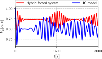
Figure 1: Probability to find the atom in its excited state $P_{e}(\alpha,t)$ with $\alpha=2$, $\omega_{c}$=1, $\omega_{a}=.95\omega_{c}$, $\omega_{L}=0.5\omega_{c}$, $\lambda=0.0125$, $\Omega=0.01$. In red we show the case for a forced system, in blue the JC model result.

In figure 1 we show the probability for the atom to be in its excited state for the hybrid pumped system (red) and for the JC Hmiltonian (blue). The initial state of the cavity is a coherent state with an average number of photons $\bar{n}=4$ and atom-cavity coupling constant $\lambda=0.0125\omega_{c}$, the pumping amplitude is $\Omega=0.01\omega_{c}$ and the atomic frequency is $\omega_{a}=0.95\omega_{c}$ with the cavity frequency set as $\omega_{c}=1$. In both cases we can see the usual pattern of quantum collapse and revivals present in the JC model, however the length of the collapse and the definition of the revivals is not the same. In the hybrid pumped case, the time between the collapse and the first revival is longer than in the JC case; the definition of the revival is more definite in the pumped case than in the JC case and the probability to find the atom in its excited state is larger for the pumped case.

Let us consider now the average value of the photon number operator; it is given by:

$$\begin{split}\langle\hat{n}(t)\rangle&=\langle\Psi(t_{0})|\hat{U}_{I}^{(1)\dagger}\hat{U}_{0}^{\dagger}\hat{n}\hat{U}_{0}\hat{U}_{I}^{(1)}|\Psi(t_{0})\rangle\\ &=\ _{I}\langle\Psi(t)|\hat{n}_{I}(t)|\Psi(t)\rangle_{I}\end{split}$$ (25)

with $\hat{n}_{I}(t)$ the photon number operator in the interaction picture. Taking the explicit form of the operator $\hat{U}_{0}$ (see Eq. 4) we obtain

$$\hat{n}_{I}(t)=\hat{n}+\beta^{*}\hat{a}+\beta\hat{a}^{\dagger}+|\beta|^{2}$$ (26)

and $|\Psi(t)\rangle_{I}$ given by Eq. 23. For the phonon number operator we get

$$\hat{N}_{I}(t)=\hat{N}+\left(\alpha_{4}\hat{b}^{\dagger}+\alpha_{4}^{*}\hat{b}\right)\hat{n}_{I}(t)+|\alpha_{4}|^{2}\hat{n}_{I}^{2}(t)$$ (27)

and we see that the phonon number operator depends on the number of photons present in the cavity. Since the pumping term modifies the photon number, then it will also modify the phonon number evolution. We can now evaluate observables like the Mandel Q parameter and the photon and phonon dispersions. We present our numerical results in the following section.

3 Numerical results, unitary evolution.

In order to test the validity of our approximations, we also made a purely numerical calculation of the average value of the photon, phonon number operators using Python [47]. In figure 2 we show the numerical and the analytical results for the temporal evolution of the photon number operator and the phonon number operator for Hamiltonian parameters specified in the caption. The evolution is done for the interval $0\leq\omega_{c}t\leq 500$ for the photons and $0\leq\omega_{c}t\leq 2000$ for the phonons. We can see an excellent agreement between the analytic and the numerical calculations. For the photons we used an initial coherent state with $\alpha=2$ and for the phonons a coherent state with $\Gamma=1$. Notice that the pumping frequency is far from the resonace cavity frequency $\omega_{c}$.

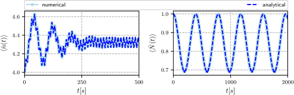
Figure 2: Temporal evolution of the photon number operator (top) and temporal evolution of the phonon number operator (bottom). Analytical results in dark-blue, numerical results in light-blue. Hamiltonian parameters $\alpha=2$, $\omega_{c}$=1, $\omega_{a}=.95\omega_{c}$, $\omega_{L}=0.5\omega_{c}$, $\omega_{m}=0.016\omega_{c}$, $G=0.00032\omega_{c}$, $\lambda=0.0125\omega_{c}$, $\Omega=0.01\omega_{c}$.

In figure 3 we show the temporal evolution of the photon number operator with initial condition $\alpha=2$ corresponding to $\langle\hat{n}\rangle=|\alpha|^{2}=4$ (top) and the probability to find the atom in its excited state (bottom). We see an exchange of excitations between the atom and the field, the probability for the atom to remain in its excited state $P_{e}(\alpha,t)$ decreases to about $0.5$ and at the same time the average number of photons increases to about 4.5, notice also the rapid oscillations with small amplitude around an average value for the number operator, these are due to the forcing term. The overall behavior of the photon number can be guessed from $P_{e}(\alpha,t)$.

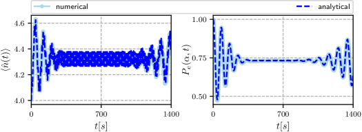
Figure 3: Temporal evolution of the photon number operator (top) and probability to find the atom in its excited state (bottom) with Hamiltonian parameters $\alpha=2$, $\omega_{c}$=1, $\omega_{a}=.95\omega_{c}$, $\omega_{L}=0.5\omega_{c}$, $\omega_{m}=0.016\omega_{c}$, $G=0.00032\omega_{c}$, $\lambda=0.0125\omega_{c}$, $\Omega=0.01\omega_{c}$. We present numerical (light-blue) and analytical (dark-blue) calculations

In figure 4 we show the temporal evolution of the average number of phonons for different amplitudes of the cavty field and Hamiltonian parameters given in the caption. The initial state of the atom is the excited state. In blue we show the case when the initial state of the field is a coherent state with $\alpha=2$ and $\langle\hat{n}(0)\rangle=|\alpha|^{2}=4$ and in green we plot the case when the initial state of the field is a coherent state with $\alpha=3$, $\langle\hat{n}(0)\rangle=9$. In both cases the initial state of the mechanical oscillator is a coherent state with $\Gamma=2$, $\langle\hat{N}(0)\rangle=4$, We have used a pump frequency near resonance $\omega_{L}=0.9\omega_{c}$. Since we are dealing with a red detuning we expect power flow from the mechanical mode to the optical mode [48] (cooling of the mechanical mode). We see that $\langle N(t)\rangle$ evolves periodically with the frequency of the mechanical oscillator, it decreases from its initial value and after a period it returns to it. Notice that the decrease is larger for the case when the average number of photons is larger so that one can manipulate the number of phonons by means of the interaction time, the amplitude of the cavity field and the frequency of the forcing term. We also show in this plot the results obtained with a purely numerical calculation and we can see a very good agreement between them.

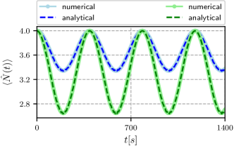
Figure 4: Temporal evolution of the phonon number operator with Hamiltonian parameters $\omega_{c}$=1, $\omega_{a}=.95\omega_{c}$, $\omega_{L}=0.9\omega_{c}$, $\omega_{m}=0.016\omega_{c}$, $G=0.00032\omega_{c}$, $\lambda=0.0125\omega_{c}$, $\Omega=0.01\omega_{c}$ and $\left\{\alpha,\Gamma\right\}=\left\{2,2\right\}$ (blue), and $\left\{\alpha,\Gamma\right\}=\left\{3,2\right\}$ (green).

To end this section we present the temporal evolution of the Mandel $Q$ parameter defined as:

$$Q(t)=\frac{\langle\hat{n}^{2}(t)\rangle-\langle\hat{n}(t)\rangle^{2}}{\langle\hat{n}(t)\rangle}-1$$ (28)

for a state with $Q$ in the range $-1\leq Q<0$ the statistics is sub-Poissonian, and if $Q>0$, super-Poissonian. For a coherent state $Q=0$. In figure 5 we plot the temporal evolution of the $Q$ function for an initial coherent state $|\alpha\rangle$ with $|\alpha|=2$. It starts at zero as corresponds to a coherent state, as time evolves it oscillates around zero alternating between positive and negative values, that is between super and sub-Poissonian statistics this happens in the same temporal region where the exchange of excitations between the field and the atom is most important. After some time it oscillates above zero with a small amplitude (when the probability to find the atom in its excited state is constant) and remains with a super-Poissonian statistics until the revival time (see figure 3) when the oscillations around zero repeat themselves.

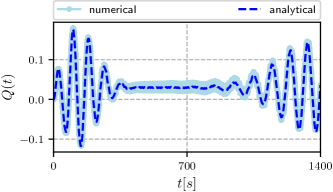
Figure 5: Temporal evolution of the Mandel parameter $Q(t)$ with Hamiltonian parameters $\omega_{c}$=1, $\omega_{a}=.95\omega_{c}$, $\omega_{L}=0.5\omega_{c}$, $\omega_{m}=0.016\omega_{c}$, $G=0.00032\omega_{c}$, $\lambda=0.0125\omega_{c}$, $\Omega=0.01\omega_{c}$ and $\alpha=2$.

4 Conclusions

In this work we have presented an approximate method to construct the time evolution operator for a hybrid system composed by a forced optomechamical oscillator and a two-level atom inside the cavity, the atom interacts only with the cavity field by means of a Jaynes-Cummings interaction. In order to solve the problem we split the Hamiltonian as the sum of a forced optomechanical Hamiltonian and that of the free atom with the JC interaction. The time evolution operator for the forced optomechanical Hamiltonian is approximated as a product of exponentials [44] and it is then used to take the JC interaction into a generalized interaction picture. As a result we obtained cumbersome expressions for the transformed operators which we approximated by neglecting terms of the order $G/\omega_{m}$ and $(G/\omega_{m})^{2}$ as compared with the cavity frequency $\omega_{c}$. Within this approximation the interaction picture Hamiltonian becomes that of a free two level atom and a displaced JC interaction whose exact time evolution operator we constructed using the Wei-Norman Theorem. Once we have the full time evolution operator we can obtain the average value of any observable, as an example we evaluated the temporal evolution of the average value of the photon and phonon number operators, the probability to find the atom in its excited state and the Mandel parameter for the cavity field. We used as initial state $|\Psi(0)\rangle=|\alpha\rangle\otimes|e\rangle\otimes|\Gamma\rangle$ where $|\alpha\rangle$ is the ket corresponding to the cavity field in a coherent state $\alpha$, $|e\rangle$ is that corresponding to the atom in its excited state and $|\Gamma\rangle$ is the ket for the mechanical oscillator in a coherent state $\Gamma$. The average number of photons is a function of the pumping amplitude $\Omega$ and the pump frequency $\omega_{L}$, when $\omega_{L}\simeq\omega_{c}$ there is a periodic growth in the number of photons and the amplitude of this growth is proportional to $\Omega$. The average number of phonons is a periodic function of time which depends also on the optomechanical coupling $G/\omega_{m}$ and on the number of photons present in the cavity. For red detuning there is a power flow from the mechanical mode to the optical mode and the cooling of the mechanical mode is more important as the number of photons increases. Since the evolution of the phonon number is periodic one can select an interaction time such that the number of phonons be at a minimum. We also evaluated the Mandel parameter for the cavity field and we found that it alternates between sub-Poissonian and super-Poissonian statistics in the region of time where there is an important exchange of excitations between the atom and the cavity field. We stress the fact that our approximations are done in the interaction Hamiltonian where we have neglected terms proportional to $G/\omega_{m}$ and $(G/\omega_{m})^{2}$ with respect to the cavity frequency $\omega_{c}$. The excellent agreement between the analytic and the numerical results obtained using the full Hamiltonian as given in (1) indicate the validity of our approximations.

Appendix A The Wei–Norman approach

Here we describe the method we used to obtain the time evolution operator for the forced optomechanical system. The first thing to notice is that the set of operators appearing in $\hat{H}_{opt}$ is closed under commutation

	$\hat{n}$	$\hat{N}$	$\hat{n}\hat{b}$	$\hat{n}\hat{b}^{\dagger}$	$\hat{n}^{2}$
$\hat{n}$	0	0	0	0	0
$\hat{N}$	0	0	$-\hat{n}\hat{b}$	$\hat{n}\hat{b}^{\dagger}$	0
$\hat{n}\hat{b}$	0	$\hat{n}\hat{b}$	0	$\hat{n}^{2}$	0
$\hat{n}\hat{b}^{\dagger}$	0	$-\hat{n}\hat{b}^{\dagger}$	$-\hat{n}^{2}$	0	0
$\hat{n}^{2}$	0	0	0	0	0

In this table, we had to incorporate the operator $\hat{n}^{2}$ that arises from the commutator between $\hat{n}\hat{b}$ and $\hat{n}\hat{b}^{\dagger}$. The time evolution operator corresponding to the Hamiltonian $\hat{H}_{opt}$ can then be written exactly as a product of exponentials [33, 49],

$$\hat{U}_{opt}(t)=e^{\alpha_{1}\hat{n}}e^{\alpha_{2}\hat{N}}e^{(\alpha_{3}+|\alpha_{4}|^{2}/2)\hat{n}^{2}}\hat{D}_{\hat{b}}(\alpha_{4}\hat{n}).$$ (A1)

The time-dependent functions $\alpha_{i}$ are obtained after substitution of Eq. A1 into Schrödinger’s equation. As a result we get:

$$\begin{split}\alpha_{1}&=-i\omega_{c}t,\\ \alpha_{2}&=-i\omega_{m}t,\\ \alpha_{3}&=-\left(\frac{G}{\omega_{m}}\right)^{2}\left[-i\omega_{m}t+\left(1-e^{-i\omega_{m}t}\right)\right],\\ \alpha_{4}&=-\frac{G}{\omega_{m}}(1-e^{i\omega_{m}t}).\end{split}$$ (A2)

Once we know the exact time evolution operator for the optomechanical system, we transform the forcing term to obtain an interaction picture Hamiltonian

$$\hat{H}_{I}^{(0)}=\hbar\Omega\cos(\omega_{L}t)\left[\hat{U}_{opt}(t)^{\dagger}(\hat{a}+\hat{a}^{\dagger})\hat{U}_{opt}(t)\right],$$ (A3)

applying the transformation we obtain:

$$\begin{split}\hat{U}_{opt}^{\dagger}\hat{a}\hat{U}_{opt}&=e^{iE(t)(2\hat{n}+1)}e^{iF(t)[\hat{b}^{\dagger}e^{i\frac{\omega_{m}}{2}t}+\hat{b}e^{-i\frac{\omega_{m}}{2}t}]}\hat{a}e^{-i\omega_{c}t},\\ \hat{U}_{opt}^{\dagger}\hat{a}^{\dagger}\hat{U}_{opt}&=\hat{a}^{\dagger}e^{i\omega_{c}t}e^{-iF(t)[\hat{b}^{\dagger}e^{i\frac{\omega_{m}}{2}t}+\hat{b}e^{-i\frac{\omega_{m}}{2}t}]}e^{-iE(t)(2\hat{n}+1)},\end{split}$$ (A4)

where

$$\begin{split}F(t)&=2\left(\frac{G}{\omega_{m}}\right)\sin\left(\frac{\omega_{m}}{2}t\right),\\ E(t)&=\left(\frac{G}{\omega_{m}}\right)^{2}(\omega_{m}t-\sin(\omega_{m}t)).\end{split}$$ (A5)

Notice the presence of the operators in the exponentials. However, the factor $G/\omega_{m}\ll 1$ [37] so that we make the approximation

$$\hat{U}_{opt}^{\dagger}\hat{a}\hat{U}_{opt}\simeq\hat{a}e^{-i\omega_{c}t},\ \ \ \hat{U}_{opt}^{\dagger}\hat{a}^{\dagger}\hat{U}_{opt}\simeq\hat{a}^{\dagger}e^{i\omega_{c}t},$$ (A6)

and, in this approximation, we get the interaction Hamiltonian

$$\tilde{H}_{I}^{(0)}=\hbar\Omega\cos(\omega_{L}t)\left(\hat{a}e^{-i\omega_{c}t}+\hat{a}^{\dagger}e^{i\omega_{c}t}\right),$$ (A7)

where we have used $\tilde{H}_{I}^{(0)}$ to denote the approximate interaction Hamiltonian. The corresponding time evolution operator can be written as a product of exponentials

$$\hat{U}_{I}^{(0)}=e^{\beta\hat{a}^{\dagger}}e^{\gamma\hat{a}}e^{\delta},$$ (A8)

with:

$$\begin{split}\dot{\beta}&=-i\Omega\cos(\omega_{L}t)e^{i\omega_{c}t},\\ \dot{\gamma}&=-i\Omega\cos(\omega_{L}t)e^{-i\omega_{c}t},\\ \dot{\delta}&=\beta\dot{\gamma},\end{split}$$ (A9)

and initial conditions $\beta(0)=\gamma(0)=\delta(0)=0.$ We see that $\beta=-\gamma^{*}$ so that we can write

$$\begin{split}\hat{U}_{I}^{(0)}&=e^{\delta}e^{\frac{1}{2}|\beta|^{2}}e^{\beta\hat{a}^{\dagger}-\beta^{*}\hat{a}}\\ &=e^{\delta+\frac{1}{2}|\beta|^{2}}\hat{D}_{\hat{a}}(\beta).\end{split}$$ (A10)

Finally, taking into account the above relationships and equation (2), the approximate evolution operator of the forced optomechanical system is [44]

$$\begin{split}\hat{U}_{0}&=\hat{U}_{opt}\hat{U}_{I}^{(0)}\\ &=e^{\delta+\frac{1}{2}|\beta|^{2}}e^{\alpha_{1}\hat{n}}e^{\alpha_{2}\hat{N}}e^{(\alpha_{3}+|\alpha_{4}|^{2}/2)\hat{n}^{2}}\hat{D}_{\hat{b}}(\alpha_{4}\hat{n})\hat{D}_{\hat{a}}(\beta).\end{split}$$ (A11)

References

- [1] E. T. Jaynes and F. W. Cummings. Comparison of quantum and semiclassical radiation theories with application to the beam maser. Proceedings of the IEEE, 51(1):89–109, 1963.
- [2] Bruce W. Shore and Peter L. Knight. The Jaynes-Cummings model. Journal of Modern Optics, 40(7):1195–1238, 1993.
- [3] Andrew D Greentree, Jens Koch, and Jonas Larson. Fifty years of Jaynes-Cummings physics. Journal of Physics B: Atomic, Molecular and Optical Physics, 46(22):220201, 2013.
- [4] J. H. Eberly, N. B. Narozhny, and J. J. Sanchez-Mondragon. Periodic spontaneous collapse and revival in a simple quantum model. Phys. Rev. Lett., 44:1323–1326, May 1980.
- [5] Gerhard Rempe, Herbert Walther, and Norbert Klein. Observation of quantum collapse and revival in a one-atom maser. Phys. Rev. Lett., 58:353–356, Jan 1987.
- [6] Serge Haroche and J-M Raimond. Exploring the quantum: atoms, cavities, and photons. Oxford university press, 2006.
- [7] Exactly soluble model of atom-phonon coupling showing periodic decay and revival. Physics Letters A, 81(2):132 – 135, 1981.
- [8] Vladimír Bužek. Jaynes-Cummings model with intensity-dependent coupling interacting with Holstein-Primakoff su(1,1) coherent state. Phys. Rev. A, 39:3196–3199, Mar 1989.
- [9] Sergio Cordero and José Récamier. Selective transition and complete revivals of a single two-level atom in the Jaynes-Cummings hamiltonian with an additional Kerr medium. Journal of Physics B: Atomic, Molecular and Optical Physics, 44(13):135502, 2011.
- [10] I. Ramos-Prieto, B. M. Rodríguez-Lara, and H. M. Moya-Cessa. Engineering nonlinear coherent states as photon-added and photon-subtracted coherent states. International Journal of Quantum Information, 12(07n08):1560005, 2014.
- [11] Michael Tavis and Frederick W. Cummings. Exact solution for an -molecule-radiation-field hamiltonian. Phys. Rev., 170:379–384, Jun 1968.
- [12] G. S. Agarwal and R. R. Puri. Collapse and revival phenomenon in the evolution of a resonant field in a Kerr-like medium. Phys. Rev. A, 39:2969–2977, Mar 1989.
- [13] M J Werner and H Risken. Q-function for the Jaynes-Cummings model with an additional Kerr medium. Quantum Optics: Journal of the European Optical Society Part B, 3(3):185–191, Jun 1991.
- [14] O de los Santos-Sánchez and J Récamier. The f-deformed Jaynes–Cummings model and its nonlinear coherent states. Journal of Physics B: Atomic, Molecular and Optical Physics, 45(1):015502, Dec 2011.
- [15] Markus Aspelmeyer, Pierre Meystre, and Keith Schwab. Quantum optomechanics. Phys. Today, 65(7):29, 2012.
- [16] T. J. Kippenberg and K. J. Vahala. Cavity optomechanics: Back-action at the mesoscale. Science, 321(5893):1172–1176, 2008.
- [17] Pierre Meystre. A short walk through quantum optomechanics. Annalen der Physik, 525(3):215–233, 2013.
- [18] Thomas Corbitt, Yanbei Chen, Edith Innerhofer, Helge Müller-Ebhardt, David Ottaway, Henning Rehbein, Daniel Sigg, Stanley Whitcomb, Christopher Wipf, and Nergis Mavalvala. An all-optical trap for a gram-scale mirror. Phys. Rev. Lett., 98:150802, Apr 2007.
- [19] Constanze Höhberger Metzger and Khaled Karrai. Cavity cooling of a microlever. Nature, 432(7020):1002–1005, Dec 2004.
- [20] J. D. Thompson, B. M. Zwickl, A. M. Jayich, Florian Marquardt, S. M. Girvin, and J. G. E. Harris. Strong dispersive coupling of a high-finesse cavity to a micromechanical membrane. Nature, 452(7183):72–75, Mar 2008.
- [21] Thomas Corbitt and Nergis Mavalvala. Review: Quantum noise in gravitational-wave interferometers. Journal of Optics B: Quantum and Semiclassical Optics, 6(8):S675–S683, jul 2004.
- [22] S. Gigan, H. R. Böhm, M. Paternostro, F. Blaser, G. Langer, J. B. Hertzberg, K. C. Schwab, D. Bäuerle, M. Aspelmeyer, and A. Zeilinger. Self-cooling of a micromirror by radiation pressure. Nature, 444(7115):67–70, Nov 2006.
- [23] Tal Carmon, Hossein Rokhsari, Lan Yang, Tobias J. Kippenberg, and Kerry J. Vahala. Temporal behavior of radiation-pressure-induced vibrations of an optical microcavity phonon mode. Phys. Rev. Lett., 94:223902, Jun 2005.
- [24] Constanze Metzger, Max Ludwig, Clemens Neuenhahn, Alexander Ortlieb, Ivan Favero, Khaled Karrai, and Florian Marquardt. Self-induced oscillations in an optomechanical system driven by bolometric backaction. Phys. Rev. Lett., 101:133903, Sep 2008.
- [25] J. I. Cirac, P. Zoller, H. J. Kimble, and H. Mabuchi. Quantum state transfer and entanglement distribution among distant nodes in a quantum network. Phys. Rev. Lett., 78:3221–3224, Apr 1997.
- [26] L.-M. Duan, M. D. Lukin, J. I. Cirac, and P. Zoller. Long-distance quantum communication with atomic ensembles and linear optics. Nature, 414(6862):413–418, Nov 2001.
- [27] K. Hammerer, M. Wallquist, C. Genes, M. Ludwig, F. Marquardt, P. Treutlein, P. Zoller, J. Ye, and H. J. Kimble. Strong coupling of a mechanical oscillator and a single atom. Phys. Rev. Lett., 103:063005, Aug 2009.
- [28] L. Slodička, G. Hétet, S. Gerber, M. Hennrich, and R. Blatt. Electromagnetically induced transparency from a single atom in free space. Phys. Rev. Lett., 105:153604, Oct 2010.
- [29] Hui Wang, Xiu Gu, Yu-xi Liu, Adam Miranowicz, and Franco Nori. Optomechanical analog of two-color electromagnetically induced transparency: Photon transmission through an optomechanical device with a two-level system. Phys. Rev. A, 90:023817, Aug 2014.
- [30] V.V. Dodonov, I.A. Malkin, and V.I. Man’ko. Even and odd coherent states and excitations of a singular oscillator. Physica, 72(3):597 – 615, 1974.
- [31] Jing Zhang, Kunchi Peng, and Samuel L. Braunstein. Quantum-state transfer from light to macroscopic oscillators. Phys. Rev. A, 68:013808, Jul 2003.
- [32] José Récamier and Rocio Jáuregui. Construction of even and odd combinations of Morse-like coherent states. Journal of Optics B: Quantum and Semiclassical Optics, 5(3):S365–S370, Jun 2003.
- [33] S. Mancini, V. I. Man’ko, and P. Tombesi. Ponderomotive control of quantum macroscopic coherence. Phys. Rev. A, 55:3042–3050, Apr 1997.
- [34] S. Bose, K. Jacobs, and P. L. Knight. Preparation of nonclassical states in cavities with a moving mirror. Phys. Rev. A, 56:4175–4186, Nov 1997.
- [35] Armando Perez-Leija, Alexander Szameit, Irán Ramos-Prieto, Hector Moya-Cessa, and Demetrios N. Christodoulides. Generalized Schrödinger cat states and their classical emulation. Phys. Rev. A, 93:053815, May 2016.
- [36] Sumei Huang and G. S. Agarwal. Enhancement of cavity cooling of a micromechanical mirror using parametric interactions. Phys. Rev. A, 79:013821, Jan 2009.
- [37] C Ventura-Velázquez, B M Rodríguez-Lara, and H M Moya-Cessa. Operator approach to quantum optomechanics. Physica Scripta, 90(6):068010, May 2015.
- [38] C. K. Law. Interaction between a moving mirror and radiation pressure: A hamiltonian formulation. Phys. Rev. A, 51:2537–2541, Mar 1995.
- [39] D. Vitali, S. Gigan, A. Ferreira, H. R. Böhm, P. Tombesi, A. Guerreiro, V. Vedral, A. Zeilinger, and M. Aspelmeyer. Optomechanical entanglement between a movable mirror and a cavity field. Phys. Rev. Lett., 98:030405, Jan 2007.
- [40] R. Ghobadi, A. R. Bahrampour, and C. Simon. Quantum optomechanics in the bistable regime. Phys. Rev. A, 84:033846, Sep 2011.
- [41] J. M. Dobrindt, I. Wilson-Rae, and T. J. Kippenberg. Parametric normal-mode splitting in cavity optomechanics. Phys. Rev. Lett., 101:263602, Dec 2008.
- [42] Hui Wang, Xiu Gu, Yu-xi Liu, Adam Miranowicz, and Franco Nori. Tunable photon blockade in a hybrid system consisting of an optomechanical device coupled to a two-level system. Phys. Rev. A, 92:033806, Sep 2015.
- [43] Devender Garg and Asoka Biswas. Coherent coupling between the motional fluctuation of a mirror and a trapped ion inside an optical cavity: Memory, state transfer, and entanglement. Phys. Rev. A, 100:053822, Nov 2019.
- [44] A Paredes-Juárez, I Ramos-Prieto, M Berrondo, and J Récamier. Lie algebraic approach to quantum driven optomechanics. Physica Scripta, 95(3):035103, Jan 2020.
- [45] B M Rodríguez-Lara and H M Moya-Cessa. The exact solution of generalized Dicke models via Susskind–Glogower operators. Journal of Physics A: Mathematical and Theoretical, 46(9):095301, Feb 2013.
- [46] I Ramos-Prieto, A Paredes, J Récamier, and H Moya-Cessa. Approximate evolution for a system composed by two coupled Jaynes–Cummings hamiltonians. Physica Scripta, 95(3):034008, Feb 2020.
- [47] J.R. Johansson, P.D. Nation, and Franco Nori. Qutip: An open-source Python framework for the dynamics of open quantum systems. Computer Physics Communications, 183(8):1760 – 1772, 2012.
- [48] T.J. Kippenberg and K.J. Vahala. Cavity optomechanics. Opt. Express, 15(25):17172–17205, Dec 2007.
- [49] J. Wei and E. Norman. On global representations of the solutions of linear differential equations as a product of exponentials. Proceedings of the American Mathematical Society, 15(2):327–334, 1964.