A Wide-area GMRT 610 MHz survey of ELAIS N1 field

Abstract

In this paper we present a wide-area 610 MHz survey of the ELAIS N1 field with the GMRT, covering an area of 12.8 deg² at a resolution of 6 arcsec and with an rms noise of $\sim 40$ $\mu$Jy beam^-1. This is equivalent to $\sim 20$ $\mu$Jy beam^-1 rms noise at 1.4 GHz for a spectral index of $-0.75$. The primary goal of the survey was to study the polarised sky at sub-mJy flux densities at $<$ GHz frequencies. In addition, a range of other science goals, such as investigations in to the nature of the low-frequency $\mu$Jy source populations and alignments of radio jets. A total of 6,400 sources were found in this region, the vast majority of them compact. The sample jointly detected by GMRT at 610 MHz and by VLA FIRST at 1.4 GHz has a median spectral index of $-0.85\pm 0.05$ and a median 610 MHz flux density of 4.5 mJy. This region has a wealth of ancillary data which is useful to characterize the detected sources. The multi-wavelength cross matching resulted optical/IR counterparts to $\sim 90$ per cent of the radio sources, with a significant fraction having at least photometric redshift. Due to the improved sensitivity of this survey over preceding ones, we have discovered six giant radio sources (GRS), with three of them at $z\sim 1$ or higher. This implies that the population of GRS may be more abundant and common than known to date and if true this has implications for the luminosity function and the evolution of radio sources. We have also identified several candidate extended relic sources.

1 Introduction

Deep and wide-area radio surveys are powerful tools to study a range of source populations. Since radio waves are not obscured by dust, deep radio surveys are also ideal to search for distant objects which are otherwise dust-obscured and thus not detected in the Ultra-violet(UV)/Optical. As can be seen from major radio surveys, the radio sky is homogeneous as compared to the optical sky (Condon, 2007). A radio survey will thus help to unveil otherwise obscured galaxy populations.

The radio sources broadly fall in two categories – normal and active galaxies. In the first case, the radio emission is due to secondary processes related to star formation such as from supernova remnants and H ii regions. Such close relation between the radio emission and star formation in normal galaxies is evident from the tight radio – infrared correlation (Condon, 1992). The radio band provides sensitive and independent estimate of star formation rate which is particularly useful where the galaxies are affected by dust obscuration and estimating star formation rate using the optical band could be affected by several observational biases. In the second case, the radio emission is due to relativistic electrons in lobes which forms the termination region of jets powered by super-massive black holes at the center of massive ellipticals. Such galaxies where there is a super-massive black hole at the centre which forms an accretion disk are known as Active Galaxies or Active Galactic Nuclei (AGN). AGNs are known to emit powerful radiation across the electromagnetic spectrum. A small fraction of them ($\sim 10$ per cent) emit powerful radio emission fueled by jets which forms hotspots and lobes on either side of the host galaxy. The size of such radio sources can be as large as several mega parsecs. The strength of radio emission in these AGNs can be several orders of magnitude more than the emission in optical band and is referred to as ‘radio loud’ AGNs (Kellermann et al., 1989). These radio loud AGNs will significantly deviate from the radio–FIR correlation. For this reason, the radio - FIR correlation is a powerful way to disentangle populations of radio sources where the emission is due to stellar origin and that due to AGN process. It has been widely accepted now that star formation is regulated or suppressed by the feedback from AGNs in galaxies (Fabian, 2012). A radio source where the radio emission is due to AGN process, naturally implies that the galaxy hosts a supermassive black hole. Therefore detecting number of radio sources where the radio emission is due to AGN process is important to understand the evolution of the host galaxy from the context of AGN feedback.

In a given radio survey where both normal galaxies and radio loud AGNs are present it is possible to classify radio sources and measure their distances through their optical counterparts. In early radio surveys such as 3CRR and 4C, most of the radio sources were radio loud AGNs. However at sub-mJy sensitivity, normal galaxies start contributing to the source population. Early deep radio surveys have helped to classify the strong radio sources ($\ga$ a few mJy) into that powered by AGNs while the faint radio sources are predominantly starbursts and normal galaxies (Windhorst et al., 1985). Since then, there have been several very deep radio surveys where the fraction of radio sources powered by AGN and starbursts were clearly identified (Padovani et al., 2011; Bonzini et al., 2013) using the tight relation between far infra-red and radio band and X-Ray data. This also helped to identify a third category of radio source where radio emission from radio quiet AGNs. As on today, it is widely accepted that at sub-mJy flux levels at 1.4 GHz, the normal galaxies dominate the radio survey where as stronger radio sources are mostly radio loud AGNs. For a statistically meaningful studies about fraction of radio loud AGNs, star forming galaxies, radio quiet AGN and other atypical radio sources deep as well as wide area surveys are required. Such surveys also have been proved useful for serendipitous discoveries of rare class of objects like relics (Brienza et al., 2016).

The radio emission is dominated by the synchrotron processes with a typical spectral index, $\alpha$, of $-$0.7 (flux density, $S$, scaling with frequency $\nu$ as $S\propto\nu^{\alpha}$). This means, for a given depth, there will be far more sources at lower radio frequencies as compared to at higher radio frequencies. In addition, a subset of radio sources preferentially show steep radio spectra with spectral index $\alpha<-1$, hence low frequency surveys are better suited to study these objects. One such population is high-redshift radio galaxies which tend to exhibit steeper radio spectra and this has been exploited to discover several high-redshift radio galaxies (Blumenthal & Miley, 1979; Ishwara-Chandra et al., 2010; Saxena et al., 2018). Therefore for discovering high-redshift radio galaxies, the radio surveys at low radio frequencies ($<1$ GHz) are preferred (Ker et al., 2012). Also, for GHz peaked spectrum sources (GPS) where the radio emission peaks at 1 to 2 GHz in rest frame, the peak is redshifted to a few hundred MHz for high redshift GPS sources (Callingham et al., 2017). In addition to such sources where low frequency will pick them up preferentially, normal radio sources will also exhibit steeper spectral index if the radio jet powering the radio lobes is switched off where the radio emitting relativistic electrons are decaying. Such steep spectral indices are characteristics of relic radio emission (Brienza et al., 2016). It has been widely believed that every AGN is likely to go through a radio loud phase which implies that radio emission from the previous epoch of activity will exhibit a steep radio spectrum and will be seen only in low frequency radio surveys. Hitherto, examples of such episodic AGNs are very scarce owing to lack of deep and wide radio surveys particularly at frequencies below 1 GHz. To summarize, low frequency radio surveys are useful to discover high-redshift radio galaxies, high-redshift GPS sources and relic radio emission due to episodic AGN activity which are often missed at GHz frequencies. Most of the deep radio surveys in the past are carried out at 1.4 GHz or higher radio frequencies which is biased against steep spectrum objects and very few deep surveys exists at $<1$ GHz with wide area and rms noise of $<0.1$ mJy beam^-1 (Bondi et al., 2007).

Here we present one of the deepest and wide area survey of ELAIS N1 region (European Large Area ISO Survey North 1) (Oliver et al., 2000) with the GMRT at 610 MHz, covering $\sim 12.8$ deg² at a resolution of 6 arcsec and with an rms noise of $\sim 40$ $\mu$Jy beam^-1. These observations are deeper than previous 610 MHz observations with the GMRT (Garn et al., 2008). For a spectral index of $-$0.75, the present observations correspond to an rms noise of $\sim 20$ $\mu$Jy beam^-1 at 1.4 GHz which is substantially deeper than VLA FIRST survey (Becker et al., 1995). Recently deeper but a smaller area of this field was observed at 400 MHz with the upgraded GMRT (Chakraborty et al., 2019). This region was chosen for several reasons such as availability of plenty of multi-wavelength data.

The paper is arranged as follows. The observations and data analysis is described in Section 2. The source catalogue is presented in Section 3. The multi-wavelength information is given in Section 4 and notes on a few individual extended objects are given in Section 5.

2 Observations and data reduction

The ELAIS N1 field was originally chosen for deep extragalactic observations with the Infrared Space Observatory (ISO) due to its low infrared background (Rowan-Robinson et al., 2004; Vaccari et al., 2005). Since then, it has gone on to become one of the best-studied 1–10 deg² extragalactic fields. The ELAIS N1 region, covering $\sim 10$ deg² was observed at 610 MHz using the Giant Metrewave Radio Telescope (GMRT). The GMRT consists of 30 antennas spread over $\sim 25$ km² area situated in western India (Swarup et al., 1991). A total of 51 pointings were employed to cover this area. The observations for most of the pointings were carried out in 2011 and 2012 and a few remaining pointings were observed in December 2017. The data were recorded using the GMRT Software Backend (GSB) with 32 MHz bandwidth and 256 spectral channels. Typically, each pointing was split over multiple days to optimise $u$-$v$ coverage. The primary calibrator 3C286 was observed on all days (additionally 3C48 on a few days) both at the start and at the end of each observing session for flux and bandpass calibration. The flux density was set using the Perley–Butler 2013 scale (Perley & Butler, 2013), with 22.179 Jy for 3C286 and 31.238 Jy for 3C48 at the channel 0 frequency of 596 MHz. Each pointing was observed for about 30 minutes and then a phase calibrator was observed for 5 minutes for gain calibrations. Total on-source time on each pointing was typically $\sim 2.5$ hours.

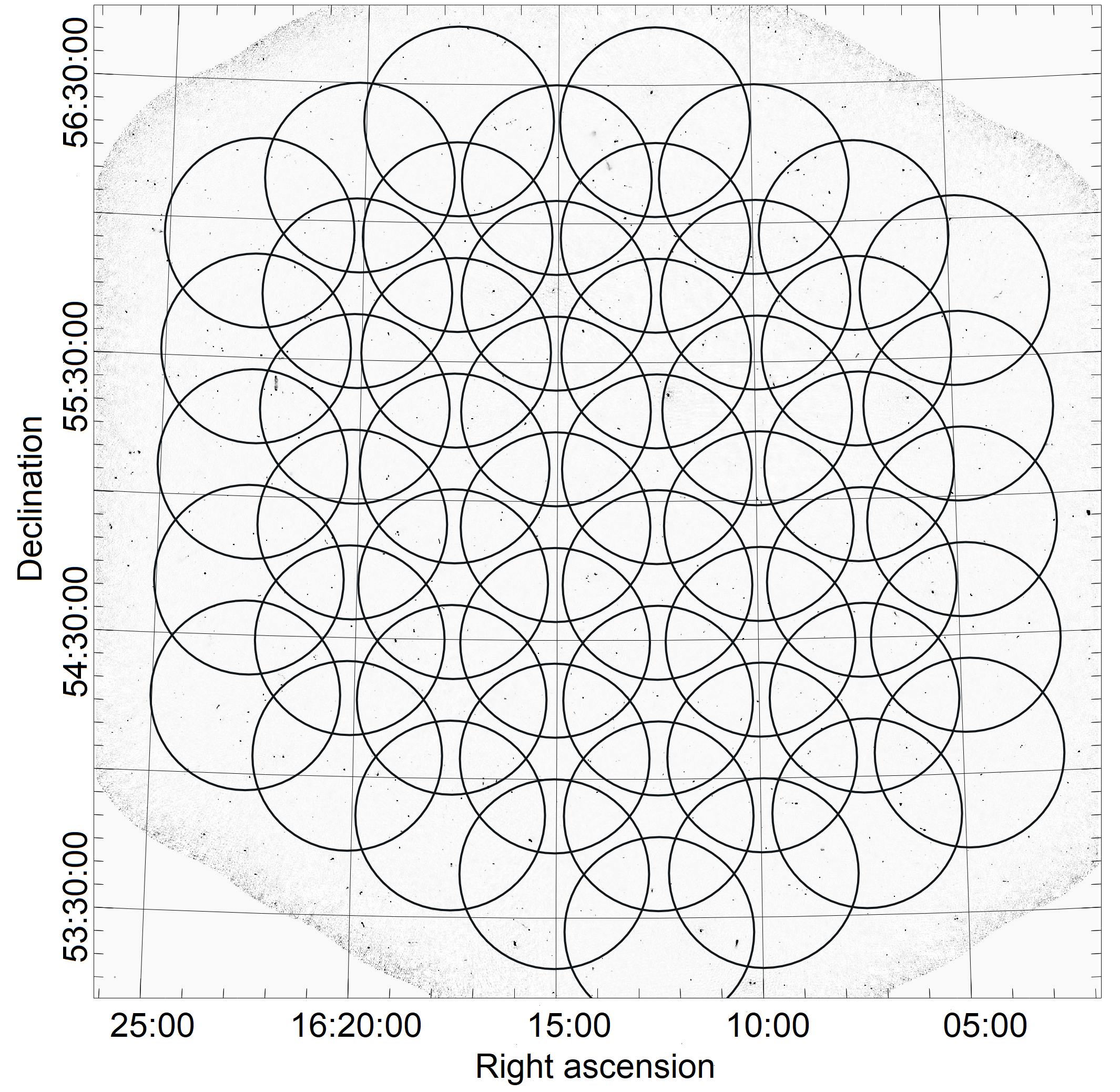
Figure 1: The array of 51 pointing centres overlaid on the ELAIS N1 610 MHz mosaic. Each pointing is represented by a circle with diameter equal to the FWHM of the primary beam of $41$ arcmin. The pointings are separated by $25$ arcmin. The area shown is $3.6\times 3.6$ deg² and the imaged portion covers 12.8 deg².

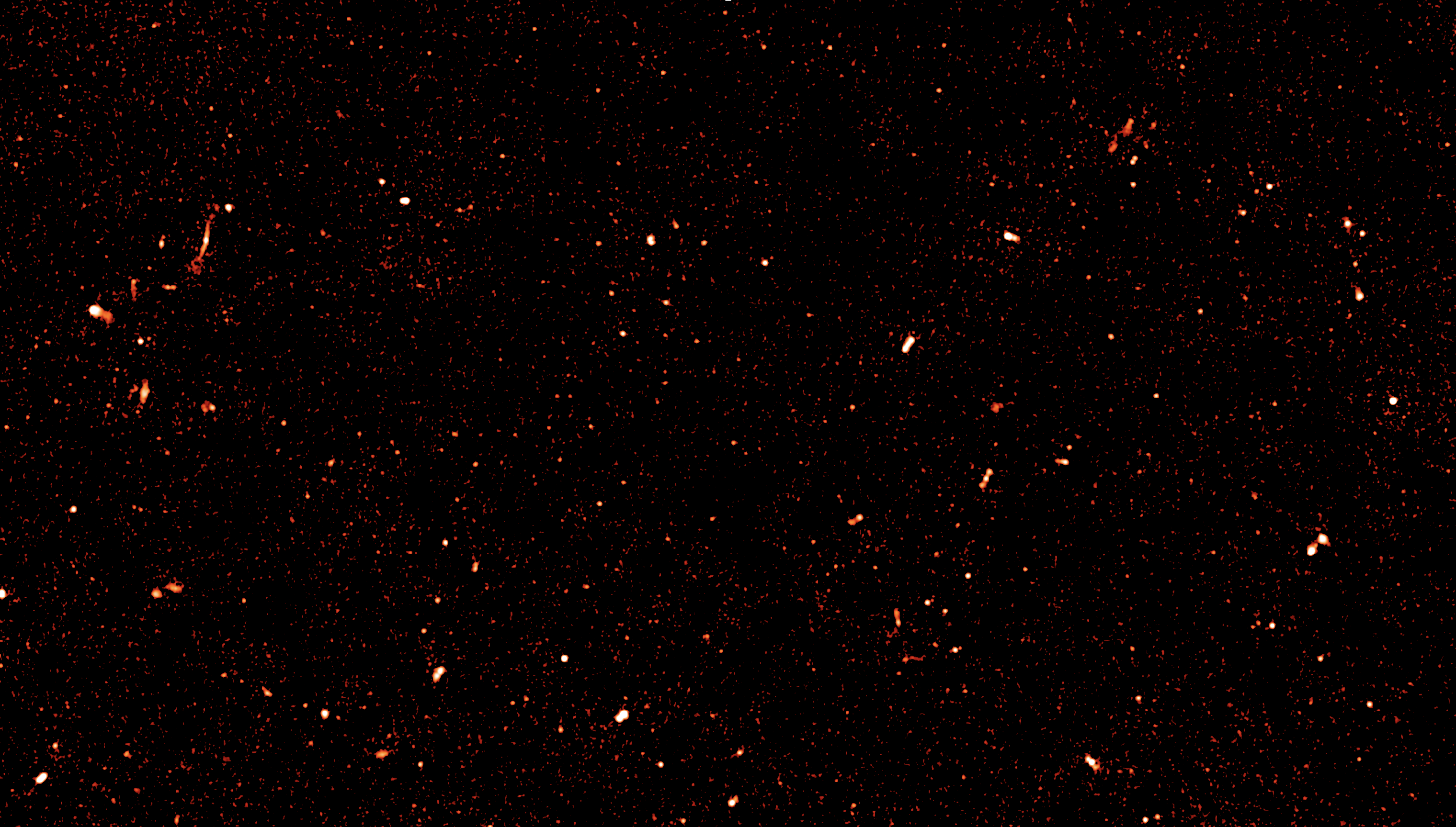
Figure 2: A $1.5\times 0.5$ deg² section of the ELAIS N1 610 MHz image centred at $\alpha=16^{\rm h}\,11^{\rm m}\,12^{\rm s}$ and $\delta=54^{\circ}\,10^{\prime}\,15^{\prime\prime}$. The resolution is 6 arcsec and the rms noise in this region of the mosaic (away from bright sources) is $\sim 40$ $\mu$Jy beam^-1. The intensity scale is logarithmic between 60 $\mu$Jy beam^-1 and 2 mJy beam^-1.

The data analysis was carried out on the data intensive cloud at the Inter-University Institute for Data Intensive Astronomy (IDIA), using a casa (Common Astronomy Software Applications) based pipeline. Initial flagging was done using the casa task flagdata. First, outliers were removed using the ‘clip’ mode and the data was flagged using the ‘tfcrop’ mode. The delay, bandpass and gain calibration were carried out on flagged data. Post-calibration, the data were flagged again, using ‘clip’, ‘tfcrop’ and ‘rflag’ modules. The data was re-calibrated after removing the initial calibration. The central $\sim$ 90% band was used for channel averaging with post-averaging channel width of 0.78 MHz to keep the bandwidth smearing negligible. On the science target, the total flagged data was $<10$ percent in most fields. Split files from each pointing (if observed on different epochs), were combined using concat before imaging. The imaging was carried out using the task tclean in casa. Four rounds of phase-only self-cal with solution intervals of 8, 4, 2 and 1 minutes and then 5 rounds of amplitude and phase self-cal with solution intervals of 8, 4, 2, 1 and 1 minutes was carried out on each pointing. The entire pipeline for calibration and imaging was carried out in nearly automatic manner. The input to the pipeline is the multi-source FITS file and other book keeping information regarding the calibrators, target name, channels to average and other imaging and calibration parameters. For convenience, the pipeline was divided into two parts as calibration and imaging. In the calibration part, the pipeline starts with importing the multi-source fits file and ends after split which produces ready-to-image calibrated visibilities. After this, common pointings observed on multiple days were concatenated (outside the pipeline) which forms the input to the imaging pipeline. A field of view of about 2.3 times the FWHM (Full Width at Half Maximum of the primary beam) was imaged to cover up to the first sidelobe. In the first round of imaging, the number of clean iterations was limited to 5000. A flux threshold of approximately 20 times the thermal noise was kept for the first round of imaging. In subsequent self-calibration and imaging rounds, the number of clean iterations was doubled with moderate lowering of the clean threshold. Also after the first round of phase-only self-calibration, flagging based on residuals (corrected_data $-$ model_data) was employed in 2nd, 3rd and fourth round of phase-only self-calibration. We have observed that the residual based flagging performs better than flagging on the corrected_data column.

After four rounds of phase-only self-calibration, the pipeline enters the amplitude-and-phase self-calibration loop. Here also, from 2nd round onwards, the data were flagged based on residuals. The total flagged data was $<30$ per cent in most fields. The final solution interval for self-calibration was limited to 1 minute in the fourth and fifth round. This resulted in significant improvement in image fidelity. The rms noise on the final individual images was $\sim 50$ $\mu$Jy beam^-1 before the primary beam correction in most of the images. Moderately higher noise was observed in fields with radio sources stronger than $\sim 100$ mJy.

The 51 pointings were mosaicked to create an image of EN1 covering an area of 12.8 deg². The mosaic geometry is illustrated in Figure 1. Due to the different $u$-$v$ coverage for each pointing, the FWHM of the synthesized beam varies between 4.5 and 6 arcsec. Before mosaicing the image from each field was smoothed to a circular Gaussian beam with FWHM of 6 arcsec. The mosaic, including data from each field up to 20 per cent level of the primary beam, was carried out in AIPS using the python script make_mosaic (Intema, private communication). The details of weighting schemes employed in the mosaic process is described in Intema et al. (2017). The final rms in the total intensity mosaic image is $\sim 40$ $\mu$Jy beam^-1. The resulting mosaic is about $3.6\times 3.6$ deg² and has total imaged solid angle of 12.8 deg² (Figure 1). A sample sub-region of the mosaic image is shown in Figure 2.

3 Source Catalogue

Table 1: A small portion of the GMRT ELAIS N1 Wide 610 MHz Source Catalogue. Full catalogue is available online.

(1)	(2)	(3)	(4)	(5)	(6)	(7)	(8)	(9)	(10)
Name	RA(J2000)	DEC(J2000)	$S_{\rm I}$	$S_{\rm p}$	RMS	$\theta_{\rm maj}$	$\theta_{\rm min}$	PA	Code
	deg$\pm$arcsec	deg$\pm$arcsec	mJy	mJy	mJy	arcsec	arcsec	deg
J161300+532637	243.24964 $\pm$ 0.46	53.44416 $\pm$ 0.50	0.55 $\pm$ 0.10	0.39 $\pm$ 0.06	0.058	7.3 $\pm$ 1.2	6.9 $\pm$ 1.1	24.7 $\pm$ 105.0	S
J161300+554834	243.24992 $\pm$ 0.35	55.80993 $\pm$ 0.34	0.27 $\pm$ 0.08	0.31 $\pm$ 0.04	0.044	6.1 $\pm$ 0.9	5.2 $\pm$ 0.7	47.1 $\pm$ 35.9	S
J161300+543542	243.25302 $\pm$ 0.28	54.59539 $\pm$ 0.32	0.34 $\pm$ 0.09	0.38 $\pm$ 0.05	0.049	6.0 $\pm$ 0.8	5.4 $\pm$ 0.6	153.5 $\pm$ 52.9	S
J161300+544502	243.25312 $\pm$ 0.59	54.75106 $\pm$ 0.54	0.36 $\pm$ 0.08	0.27 $\pm$ 0.05	0.050	7.4 $\pm$ 1.5	6.4 $\pm$ 1.1	54.7 $\pm$ 59.0	S
J161300+555238	243.25336 $\pm$ 0.73	55.87776 $\pm$ 1.95	4.44 $\pm$ 0.20	1.25 $\pm$ 0.14	0.082	23.6 $\pm$ 4.9	5.7 $\pm$ 0.6	70.5 $\pm$ 8.9	M
J161300+534130	243.25364 $\pm$ 0.06	53.69203 $\pm$ 0.06	1.83 $\pm$ 0.08	1.68 $\pm$ 0.06	0.038	6.4 $\pm$ 0.1	6.1 $\pm$ 0.1	68.6 $\pm$ 22.6	S
J161301+541001	243.25443 $\pm$ 0.12	54.16748 $\pm$ 0.14	0.97 $\pm$ 0.07	0.83 $\pm$ 0.05	0.038	6.7 $\pm$ 0.3	6.3 $\pm$ 0.3	178.4 $\pm$ 29.5	S
J161301+535251	243.25504 $\pm$ 0.22	53.88111 $\pm$ 0.24	0.31 $\pm$ 0.06	0.36 $\pm$ 0.04	0.036	5.7 $\pm$ 0.6	5.4 $\pm$ 0.5	169.9 $\pm$ 89.5	S
J161301+533521	243.25613 $\pm$ 0.42	53.58959 $\pm$ 0.26	0.33 $\pm$ 0.07	0.32 $\pm$ 0.04	0.041	7.0 $\pm$ 1.0	5.3 $\pm$ 0.6	103.8 $\pm$ 20.9	S
J161301+533851	243.25670 $\pm$ 0.30	53.64803 $\pm$ 0.89	0.46 $\pm$ 0.10	0.24 $\pm$ 0.04	0.042	8.2 $\pm$ 2.2	2.9 $\pm$ 0.2	72.2 $\pm$ 7.0	M

The source catalogue was created using PyBDSF (Mohan & Rafferty, 2015). In order to minimise the possibility of spurious candidates near bright sources and at the edge, we have adopted advanced options. Near the bright sources we have adopted a smaller rms box size of $33\times 33$ pixel² sliding by 11 pixels. In the rest of the image, the rms box size of $40\times 40$ pixel² sliding by 13 pixels was used. This scheme resulted in least number of spurious sources near bright sources on visual inspection, as compared to other box sizes that were tried. For source detection, a 5$\sigma$ threshold for peak pixel and 3$\sigma$ cutoff for island boundary was used. We had invoked the option to group overlapping Gaussians into a single source. With these criteria, a total of 6,474 sources were catalogued. All the sources were visually inspected and 74 sources which were likely to be noise peaks in the high noise region near bright sources were removed.

In Figure 3 we plot the ratio of total flux density to peak intensity against the significance of detection ($S_{peak}/\sigma$). In order to fit an envelope to $S_{peak}/\sigma$ as a function of source flux, we divided the data into several bins with closer spacing at lower significance and fewer bins at higher significance to check the distribution of sources. In each bin there were a few out-liers with $S_{\rm tot}/S_{\rm peak}<1$. To exclude these out-liers, we considered the ratio of total to peak where the distribution started to become continuous and this value was taken as the lower envelope. We fitted a profile to this envelope with the function $1.0+(1.88\pm 0.10)/x$, where $x$ is $S_{peak}/\sigma$. The envelope is shown in the figure. All the points that fall within this envelope on both sides are taken as point sources. With this criterion, about 60 per cent of sources are unresolved. If we were to consider the total to peak flux ratio $<1.5$ as compact sources then the number of compact sources are 4,790 ($\sim 75$ per cent).

Table 1 lists the ten entries of the source catalogue. The columns contain: (1) the source name JHHMMSS+DDMMSS, where HHMMSS are the hours, minutes and seconds of time of right ascension and DDMMSS are the degrees, minutes and seconds of arc of declination (both in J2000), (2) the J2000 right ascension (degrees) and error (arcseconds), (3) the J2000 declination (degrees) and error (arcseconds), (4) the integrated Stokes $I$ flux density and error (mJy), (5) the peak Stokes $I$ intensity and error (mJy beam^-1), (6) the rms at the source position (mJy) returned by PyBDSF, (7 and 8) the dimensions of the fitted major and minor axes of 2D Gaussian with errors (arc seconds), (9) the position angle of the source major axis (degrees) with respect to north, and (10) the source classification code, as in (Mohan & Rafferty, 2015). All errors are $1\sigma$. Errors on flux density include a contribution of 2.6% derived as the percent rms variation of the calibration solution for the flux of the secondary calibrator 1549+506 over the 23 different observing sessions. This error was added in quadrature to the PyBDSF measurement error. The full source catalogue is available in machine readable form.

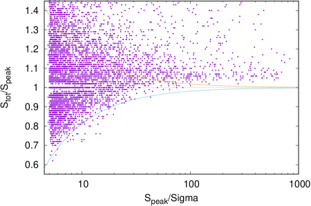
Figure 3: The plot showing the ratio of the integrated flux density to peak intensity as a function of the significance of detection. Inorder to highlight the distribution near the ratio of 1, the y-axis has been restricted in the range 0.5 to 1.5.

3.1 Spectral index of compact sources

We have used the compact sources ($S_{\rm tot}/S_{\rm peak}<1.5$) to check for spectral index w.r.t. VLA FIRST at 1.4 GHz and the GMRT 325 MHz catalogue from (Sirothia et al., 2009). The median spectral index w.r.t. VLA FIRST 1.4 GHz is $-0.85\pm 0.05$ and w.r.t. 325 MHz is $-0.73\pm 0.12$. The spectral index distribution between our 610 MHz and the VLA FIRST 1.4 GHz observations is shown in Figure 4. The median 610 MHz flux density of sources with a VLA FIRST counterpart is 4.5 mJy, whereas the median 610 MHz flux density of sources with a GMRT 325 MHz counterpart is 0.72 mJy. The GMRT 325 MHz observations covers a smaller region ($\sim 1.5$ deg²). Recently, higher sensitivity data from the upgraded GMRT at band-3 (250-500 MHz) has been published (Chakraborty et al., 2019). The median spectral index using these data is $0.70\pm 0.18$. The steeper spectral index for brighter sources and relatively flatter spectral index for fainter sources is also seen in other samples (Whittam et al., 2013; Mahony et al., 2016).

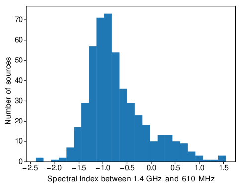
Figure 4: The spectral index distribution between 610 MHz and 1.4 GHz. The median spectral index is $-0.85\pm 0.05$.

3.2 Source Counts

The large area and sub-mJy depth of the observations allows us to derive source counts with low statistical errors down to $\sim 200$ $\mu$Jy. However systematic effects become a significant factor at intermediate signal-to-noise levels. For flux limited observations in the presence of noise, the two important effects are Eddington bias (Eddington, 1913), and incompleteness of the sample at faint flux densities. Eddington bias arises due to the effects of the noise distribution on the measured flux densities of the underlying ensemble of radio sources, which distorts the observed flux density distribution relative to the true flux density distribution. Eddington bias corrections generally assume that the noise is well described by a normal distribution (Eddington, 1940). However for wide-field radio mosaic images the effect of image noise on the detected source fluxes will differ from a simple normal distribution, due both to the change in background image rms with position arising from the spatial variation of the mosaic weights, and to the non-Gaussian increase of the background rms in the vicinity of bright sources caused by residual deconvolution errors.

The observed differential source counts can be related to the true source counts as

$$\frac{{\rm d}N_{\rm o}(s^{\prime})}{{\rm d}s^{\prime}}=\int_{0}^{\infty}\frac{{\rm d}N_{\rm t}(s)}{{\rm d}s}\,\epsilon(s)\,p(s,s^{\prime})\,{\rm d}s$$ (1)

Here ${\rm d}N_{\rm o}(s^{\prime})/{\rm d}s^{\prime}$ is the observed count at the observed flux densities $s^{\prime}$, and ${\rm d}N_{\rm t}(s)/{\rm d}s$ is the true source count at the true flux density $s$. The function $p(s,s^{\prime})$ is the normalized probability density function that a source at observed flux $s^{\prime}$ is due to a source with true flux density $s$, and $\epsilon(s)$ is the probability that a source with true flux density, $s$, will result in a detection.

We measure both $p(s,s^{\prime})$ and $\epsilon(s)$ by injecting sources into the PyBDSF residual image - the image with the fits to the detected radio sources removed. For true flux density $s$ ranging from below the noise to several mJy, we injected 3000 sources at fixed values of true flux density with the dimension of the synthesized beam. We do not consider resolved sources in this analysis as we expect the dominant source population at sub-mJy flux densities is a combination of star forming galaxies and radio quiet AGN (Ocran et al., 2020), which will be unresolved at angular resolution of several arc seconds. These injected sources populate an image with the same background noise and rms properties as the original source finding. We then ran PyBDSF on the images with injected sources and measured the fraction of sources detected as a function of true flux, and the distribution of true flux densities of injected sources that result in a source with observed flux $s^{\prime}$. Figure 5 shows the detection efficiency function $\epsilon(s)$. The data points are the results for each simulation of 3000 sources, and the solid line is a piece-wise polynomial spline interpolation of the data. The vertical dashed line in the Figure 5 is the approximate $5\sigma$ detection threshold. Sources with true flux well below the threshold can produce detections because some fraction of the sources have their ‘observed’ flux density increased above the threshold according to $p(s,s^{\prime})$. As expected the functions $p(s,s^{\prime})$ are generally non-Gaussian in shape.

Figure 6 shows an example of the shape of the function for the case of $s^{\prime}=380$ $\mu$Jy beam^-1. The function is skewed, with a negative tail toward lower flux densities. We fit a skew normal distribution to the data as shown by the dashed line in Figure 6. A skew normal is described as

$$f(x)=\frac{2}{\omega}\phi(x)\Phi(\gamma x)$$ (2)

where

$$\phi(x)=\frac{1}{\sqrt{2\pi}}{\rm e}^{-\frac{x^{2}}{2}},\quad{\rm and}\quad\Phi(\gamma x)=\frac{1}{2}\left[1+{\rm erf}\left(\frac{\gamma x}{\sqrt{2}}\right)\right]$$ (3)

The skew parameter, $\gamma$, is zero for a symmetric normal distribution. The parameters of the skew normal distribution are fit to the data as a function of $s^{\prime}$, so $\gamma=\gamma(s^{\prime})$ and

$$x=\frac{s-\xi(s^{\prime})}{\omega(s^{\prime})}$$ (4)

This allows the probability density distribution $p(s,s^{\prime})$ to be constructed for any value of $s^{\prime}$ and $s$, and together with $\epsilon(s)$ allows an predicted observed source count to be derived from the a true source count using the integral Equation 1. We solve for the combined completeness and bias correction by first setting the true count equal to the observed count and iteratively modifying the trial true count until the left hand side of Equation 1 equals the observed counts. We then derive a per-bin correction to the observed counts. The resulting source counts are listed in Table 2 and plotted in Figure 7. Our counts lie near the middle of the scatter of other observed counts at 610 MHz (Bondi et al., 2007; Garn et al., 2008; Ocran et al., 2020). The scatter of the observations of about a factor of two below 1 mJy, is similar to the scatter in model counts shown on the plot (Wilman et al., 2008; Massardi et al., 2010; Bonaldi et al., 2019).

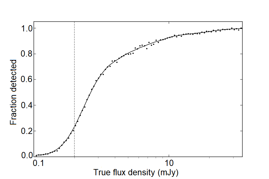
Figure 5: Fraction of sources detected as a function of true flux density. The data points are the results of simulations described in the text. The solid line is model fit based on piece-wise polynomial spline interpolation of the simulated data. The vertical dashed line shows the approximate $5\sigma$ detection level of 200 $\mu$Jy beam^-1.

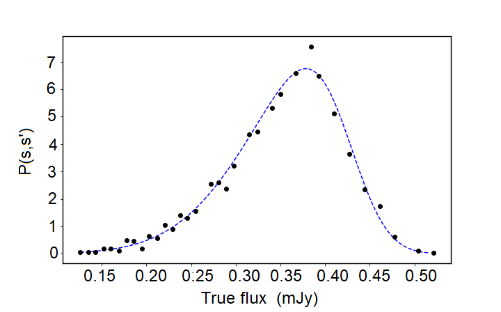
Figure 6: An example probability density distribution $p(s,s^{\prime})$ for $s^{\prime}=380$ $\mu$Jy. The dashed line is a skew normal distribution fit to the simulations (data points).

Table 2: Euclidean normalized 610 MHz source counts within the ELAIS N1 Wide field

Mean Flux	Bin Width	$N$	Count	Error
(mJy)	(mJy)		(Jy1.5 sr-1)	(Jy1.5 sr-1)
0.239	0.043	510	7.65	0.34
0.285	0.052	664	8.55	0.33
0.341	0.062	705	8.80	0.33
0.408	0.075	626	8.63	0.35
0.489	0.090	525	8.46	0.37
0.589	0.107	412	8.44	0.42
0.702	0.129	344	8.58	0.46
0.849	0.155	289	9.14	0.54
1.010	0.186	246	9.77	0.62
1.223	0.223	237	12.64	0.82
1.459	0.267	151	10.44	0.85
1.766	0.321	155	14.39	1.16
2.113	0.385	112	13.57	1.28
2.538	0.462	121	19.30	1.75
3.063	0.555	95	20.22	2.07
3.641	0.666	96	26.22	2.68
4.370	0.799	83	29.82	3.27
5.208	0.958	77	35.75	4.07
6.213	1.150	57	34.27	4.54
7.554	1.380	47	38.39	5.60
9.147	1.656	48	52.70	7.61
11.113	1.987	50	74.44	10.53
12.743	2.385	47	82.10	11.99
15.893	2.862	38	96.10	15.59
18.897	3.434	36	116.92	19.49
22.314	4.121	31	127.16	22.84
27.144	4.945	32	178.52	31.56
32.047	5.934	23	161.94	33.77
39.030	7.121	15	144.07	37.20
46.524	8.546	23	285.57	59.55
55.476	10.255	25	401.63	80.33
67.533	12.306	11	240.79	72.60
81.071	14.767	9	259.22	88.41
96.641	17.720	11	409.62	123.50

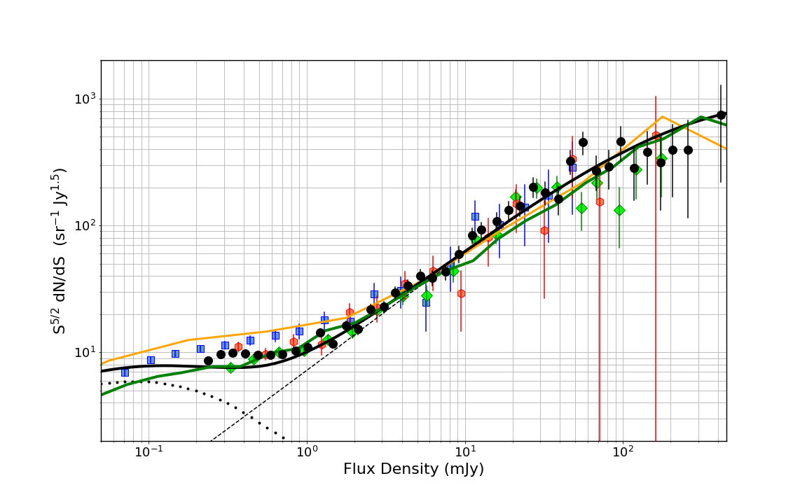
Figure 7: Radio source counts at 610 MHz. Counts from this work are shown as filled black circles. Red hexagons are counts from Bondi et al. (2007), and green diamonds are from Garn et al. (2008). The blue squares are the recent results of very deep GMRT imaging by Ocran et al. (2020). For comparison, the solid lines show model predictions for 610 MHz counts from Wilman et al. (2008) (green), Massardi et al. (2010) (black), and Bonaldi et al. (2019) (orange). The dotted and short dashed lines show indicative model counts for starburst galaxies and AGN from Massardi et al. (2010).

3.3 Multi-Wavelength counterparts and redshift distribution

The extensive multi-wavelength data available within the ELAIS N1 field has been collected and homogeneized over the last few years. The Spitzer Data Fusion (Vaccari et al., 2010; Vaccari, 2015) project has produced Spitzer-selected multi-wavelength catalogues for 8 extragalactic survey fields and a total of 65 deg² covered in the 7 IRAC and MIPS bands. The Herschel Extragalactic Legacy Project (Vaccari, 2016; Małek et al., 2018; Shirley et al., 2019) has produced multi-wavelength catalogues for sources over the 1,300 deg² of the extragalactic sky covered by Herschel. For this work, we have used data products from both projects to optimize the multi-wavelength source characterization process. In order to minimize the ambiguity of the identification, we have matched radio sources with their Spitzer/SWIRE mid-infrared and UKIDSS DXS near-infrared (where a Spitzer/SWIRE counterpart was not found) counterparts using a nearest-neighbour technique with a search radius equal to three times the estimated astrometric error. We have combined the spectroscopic redshift compilations from the Spitzer Data Fusion and HELP projects to collect spectroscopic redshifts. Where a spectroscopic redshift was not available, we have used photometric redshifts from (in order of preference) the HSC (Tanaka et al., 2018), SWIRE (Rowan-Robinson et al., 2008; Rowan-Robinson et al., 2013), HELP (Duncan et al., 2018a; Duncan et al., 2018b), SERVS (Pforr et al., 2019) and SDSS (Beck et al., 2016) projects. The redshift distribution is illustrated in Figure 8.

Multi-wavelength coverage and matching statistics are summarized in Table 3. We find that 86.3% of the GMRT footprint is covered by either SWIRE or UKIDSS, and within this common footprint we find that 91.9% of our sample finds a match and 74.4% a redshift estimate. At the flux density limits of our radio survey and of our multi-wavelength datasets, we expect the overwhelming majority of radio sources to have an infrared counterpart, and indeed the vast majority of unmatched sources fall outside the SWIRE and UKIDSS coverage. Of the $\sim 8$% sources which does not have counterparts, the majority of them could be the Infrared Faint Radio Sources (IFRS) (Norris et al., 2011), however, some of them could also be the lobes of active galaxies. We have not investigated unmatched radio sources within the SWIRE/UKIDSS coverage individually as a full multi-wavelength analysis is outside the scope of the present paper. However, a cursory inspection of a few unmatched radio sources confirms that, as also found by Ocran et al. (2017, 2020), most of them are in ‘complex’ areas of the radio or of the infrared images and thus do not lend themselves to being identified via an automated procedure.

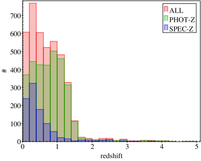
Figure 8: The Redshift Distribution of GMRT Sources.

Table 3: Multi-Wavelength Data for GMRT Sources.

Catalogue	No. of Sources	Fraction
GMRT	6400	100$\%$
COVERED-ALL	5523/6400	86.3$\%$
COVERED-SWIRE	5473/6400	85.5$\%$
COVERED-UKIDSS	5024/6400	78.5$\%$
MATCHED-ALL	5078/5523	91.9$\%$
MATCHED-SWIRE	4945/5473	90.4$\%$
MATCHED-UKIDSS	4029/5024	80.2$\%$
SWIRE IRAC1234	2827/5523	51.2$\%$
SWIRE MIPS24	3408/5523	61.7$\%$
X-RAY	59/5523	1.1$\%$
SPECZ	970/5523	17.6$\%$
PHOTZ	3138/5523	56.7$\%$
REDSHIFT (ANY)	4108/5523	74.4$\%$

Figure 9: Giant Radio Sources discovered in our ELAIS N1 wide area survey. Top row from left: Giant radio galaxies J1613+5616, 1607+5447, J1611+5432 and J1608+5434. Bottom row: Giant radio quasars J1609+5354 (GMRT 610 MHz), J1609+5354 (VLA FIRST 1.4 GHz) and J1608+5611.

4 Giant Radio Sources

During the visual inspection of the ELAIS N1 field for large angular sized sources, we have discovered several giant radio sources (GRS) with linear size of over a Mpc. GRS are believed to be the late stage in the evolution of radio galaxies (Ishwara-Chandra & Saikia, 1999) and hence finding more number of GRSs in the sky is important to shed light on possible scenarios that can explain the formation and evolution of GRS (Dabhade et al., 2020). The number of known GRS have dramatically increased in recent years due to careful investigation of wide area sky surveys in the radio and availability of redshifts from optical surveys such as SDSS (Proctor, 2016; Dabhade et al., 2017, 2020). The apparent low space density of GRSs may be due to lack of sensitive wide area surveys (Kaiser et al., 1997).

In the ELAIS N1 field, we found five objects with linear size of $\sim$ a Mpc or larger and one object with a linear size of 0.85 Mpc. This is among the highest number density of GRSs in a deep field, comparable to the number density of GRSs in Dabhade et al. (2020). Most of the GRS discovered from this work are too faint to be detected in the existing surveys such as VLA FIRST and NVSS. It appears now that GRSs are more common than indicated by earlier studies (Kaiser et al., 1997), highlighting the importance of sensitive wide area survey to discover more such objects.

Here we briefly describe the properties of individual giant sources. The redshifts were obtained from NASA/IPAC Extragalactic Database (NED) at the position of the core.

J1613$+$5616

This is a low redshift GRS at $z=0.18$ (Figure 9, top left panel). The angular size is $\sim 8.5$ arcmin which makes the linear size 1.5 Mpc. The flux density of the core is 11.5 mJy at 610 MHz, 7.8 mJy from VLA FIRST at 1.4 GHz and 8.7 mJy in NVSS at 1.4 GHz. Due to the large angular size of the object and high angular resolution, the lobes are highly resolved, and hence the total flux density may be underestimated due to missing flux. The spectral index of the core is flat suggesting a currently active AGN, despite its large size. Assuming a hotspot advance speed of $\sim 0.1c$ gives the kinematic age as $\sim 50$ million years. Midway to the hotspots, two peaks are seen roughly equidistant from the core, at $16^{\rm h}13^{\rm m}57\aas@@fstack{s}3$ and $+56^{\circ}17^{\prime}23\aas@@fstack{\prime\prime}6$ in the northern side and at $16^{\rm h}13^{\rm m}46\aas@@fstack{s}6$ and $+56^{\circ}13^{\prime}47\aas@@fstack{\prime\prime}8$ in the southern direction. Such structures could normally suggest the source to be a double-double radio source, however it is puzzling to see this ‘inner pair’ much weaker than the outer pair, if this is true. The absence of bright outer hotspots, flat-spectrum core and large kinematic age does support the double-double source possibility. Spectral index information of the inner and outer structures are needed to conclude the double-double nature of the source.

J1607$+$5447

The angular size of the source is 2.5^′ (Figure 9, top panel, second from left). For this size, it will be a GRS with size $>1$ Mpc for any redshift above 0.6. The HSC Photometric redshift of this source is 1.14 and the corresponding linear size of the source is 1.25 Mpc, classifying this as a giant radio source. The lobes are faint and the emission is confined to largely near the hotspots. In the VLA FIRST survey, only the core is detected, with a flux density of 2.5 mJy. The flux density of the core at 610 MHz is 2.8 mJy.

Figure 10: A few radio sources with peculiar morphologies and candidate relic AGNs. Top left: J1617+5432, top middle: J1611+5559, top right:J1621+5518.Bottom left: GMRT 610 MHz image of J1613+5608 and to right the VLA FIRST image of this source to highlight the non-detection of west-lobe at 1.4 GHz.

J1611$+$5432

The spectroscopic redshift of this source (Figure 9, top panel, third from left) is 0.714 and for the angular size 2.2^′, the linear size is 0.95 Mpc, hence we included this in the category of GRS 9. Only the southern lobe is detected in VLA FIRST, but both lobes are detected in the NVSS with a flux density of 4 mJy for the southern lobe and the northern lobe at 2.9 mJy. The corresponding values at 610 MHz are 11.9 mJy and 5.9 mJy respectively. The southern lobe has a steeper spectral index of $-1.3$ as compared to the northern lobe ($-0.9$).

J1608$+$5434

The host galaxy of this GRS lies at spectroscopic redshift of 0.909. The angular size 1.8 arcmin of the source corresponds to a linear size of 0.85 Mpc Figure (9, top panel, last). The core and southern lobe are blended in the NVSS and hence this appears as a double source in NVSS. Though the size is $<1$ Mpc, we have included this source here due to its higher redshift since there are very few GRS known in this redshift range.

J1609$+$5354

This giant radio quasar (Figure 9, bottom left panel) has a spectroscopic redshift of 0.99258. The source is about 2.5^′ in size which translates to a linear size of 1.1 Mpc. There are several interesting features for this giant radio quasar. There are structures present in both the lobes, which suggests more than one hotspot. Recently Krause et al. (2019) have studied a sample of powerful radio sources and modelled sources with such structures as due to precessing jets and speculated that such phenomena may be more common in radio loud AGNs. The other interesting aspect of this source is that the east lobe is resolved out in VLA FIRST (Figure 9, bottom middle panel), despite the fact that both our 610 MHz image and VLA FIRST have comparable angular resolution. The spectral index scaled equivalent rms noise at 1.4 GHz is $\sim 20$ $\mu$Jy beam^-1 for our 610 MHz images, which makes it much deeper than VLA FIRST, hence the clear detection of the east lobe with 610 MHz GMRT. This lobe is barely detected in the NVSS with flux density of 4.7 mJy. At 610 MHz the integrated flux density is 9.3 mJy, resulting in a spectral index of $-0.8$ for this lobe.

The west lobe is much brighter with flux density of 130 mJy at 610 MHz and 58 mJy at 1.4 GHz from the NVSS. The spectral index is about $-1$, steeper than that observed for lobes of other radio quasars. Such a steeper spectral index for lobes of high redshift radio sources could also arise due to increased energy loss via the inverse-Compton mechanism.

The flux density of the core is 40.8 mJy at 610 MHz, 43.8 mJy at 1.4 GHz from VLA FIRST and 45.2 mJy at 1.4 GHz from the NVSS. The spectral index of the core is thus flat, which is common for powerful radio quasars. The total radio luminosity of this source at 1.4 GHz is $5.7\times 10^{26}$ W Hz^-1.

J1608$+$5611

This is among the highest redshift giant radio quasars at a redshift of 1.32 (Figure 9, bottom right panel). The angular size is 2.6^′ which corresponds to a linear size of 1.3 Mpc. The armlength on the east is much longer than the west side resulting in a highly asymmetric axial ratio. The core has flat spectrum. The total radio power is comparable to the GRS J1609$+$5354.

Figure 11: Some nearby galaxies where extended radio emission is seen. Top Left: NGC 6143. Top right: CGCG 276-004. Bottom left: GALEXMSC J160603.68$+$552527.9. Bottom right:2MASX J16142202$+$5432180.

5 Other Peculiar sources

In this section we discuss a few sources which are likely to be relic sources or sources with very diffuse emission. These sources have been selected by visually inspecting the image for extended morphology at 610 MHz. The purpose of this section is to highlight the possibility of discovering peculiar sources and relics in the wide and deep radio surveys.

J1617$+$5432

This is a ‘compact’ double–double radio source (Figure 10, top left panel). The optical counterpart is located at the central region of the inner double and has a spectroscopic redshift of 0.6999. The total angular size of the source is less than an arcmin and hence the structure is not resolved in the NVSS. The total flux density at 610 MHz is 10.7 mJy and at NVSS is 4.5 mJy which corresponds to a spectral index of $-1.0$. In the VLA FIRST survey, only the inner compact hotspot pair is detected with total flux density of 4 mJy. The radio morphology has two distinct emission regions, the outer lobes are diffuse compared to compact inner lobes. The presence of a clear compact hotspot pair in VLA FIRST further supports that this is a re-started AGN. Since most of the double-double radio sources known today are large angular size, the discovery of such relatively compact sources with episodic activity may point to the scenario where the signatures of episodic activity may be more common with shorter duty cycle.

J1611$+$5559

This is a very compact double having an angular extent less than 0.5^′ (Figure 10, top middle panel). The redshift of the galaxy is 0.314. The total flux density at 610 MHz is 15.7 mJy. The source is not catalogued in the VLA FIRST. We have inspected the VLA FIRST image as well as our VLA image at 1.4 GHz with marginally higher resolution but with comparable rms noise to VLA FIRST. A compact pair of hotspots separated by about 6^′′, aligned in the north-east direction is seen. We have estimated the flux around this using the AIPS task TVSTAT which yielded a flux density of 3.6 mJy. The source is detected in the NVSS with a flux density of 4.8 mJy which puts the spectral index between 610 MHz and 1.4 GHz at $-1.4$. This is a clear indication of presence of relic emission.

J1621$+$5518

The flux ratio between the two lobes is $>20$, making this one of the most asymmetric doubles (Figure 10, top right panel). A faint compact radio source is detected roughly one-third distance to the north-west lobe and it has optical counterpart in the SDSS with photometric redshift of 0.569. The flux density of the south-east lobe at 610 MHz is 25.4 mJy and at 1.4 GHz (NVSS) is 10.0 mJy. The flux density of north-west lobe is 2.1 mJy at 610 MHz and not detected in our VLA image as well as VLA FIRST.

J1613$+$5608

The radio morphology appears ‘normal’ in the first look, but when investigated in detail, this source has some interesting features (Figure 10, bottom left panel). The SDSS galaxy SDSS J161312.25$+$560800.5 with photometric redshift of 0.2 at the ‘expected’ location could be a possible core - there is no other galaxy or quasar in the central region. The west lobe is resolved out in the VLA FIRST survey (Figure 10, bottom right panel). The total flux density at 610 MHz for the west lobe is 8.8 mJy and the NVSS flux density is 3.2 mJy which gives a steep spectral index of $-1.2$. For the east lobe the 610 MHz flux density is 18.4 mJy and at NVSS it is 6.5 mJy which again gives a steep spectral index of $-1.2$ for this lobe. Another interesting feature of this source is knot like structures in the jet that are midway to the hot spot on either side.

J1615+5452

This is a remnant radio AGN without any compact feature. Multi-frequency analysis of this AGN has been presented in Randriamanakoto et al. (2020).

6 Nearby galaxies

Here we discuss a few regular nearby star forming galaxies showing extended morphology at 610 MHz.

NGC 6143

NGC 6143 is a face on spiral galaxy at a redshift of 0.0177 (Figure 11, top left panel). We have detected extended radio emission from this galaxy at 610 MHz. This source was not catalogued with PyBDSF due to its low surface brightness and the smaller rms box size we adopted in PyBDSF. The integrated flux density at 610 MHz is 13.2 mJy excluding the point source at the edge. The source is detected in the NVSS with flux density of 6.2 mJy. The point source is not detected in the VLA FIRST survey and in the high resolution VLA survey by this team, hence its contribution at 1.4 GHz is negligible. The spectral index of the source comes to be $-0.9\pm 0.2$. The slightly steeper spectral index is consistent with the steeper spectral index observed for halo emission at low radio frequencies in nearby galaxies such as NGC 891 (Hummel et al., 1991).

CGCG 276$-$004

CGCG 276-004 is another face on spiral galaxy at redshift of 0.0529 which has been clearly detected in our observations (Figure 11, top right panel). This lies in a galaxy group (Tully, 2015). The integrated flux density is 12.8 mJy at 610 MHz. The source has been detected in NVSS with a flux density of 5.8 mJy. The radio spectral between 610 MHz and 1.4 GHz is $-0.95\pm 0.2$ which is similar to NGC 6143 discussed in the previous section.

GALEXMSC J160603.68$+$552527.9

This galaxy (Figure 11, bottom left panel) is at redshift of 0.0311 and SDSS classified it as ‘broad line galaxy’. This object has not been studied in detail in the literature. The radio emission is extremely diffuse and faint. The integrated flux density at 610 MHz is 10 mJy. The galaxy is detected in the NVSS with a flux density of 7.4 mJy. The spectral index is much flatter than NGC 6143 and CGCG 276-004. This could be due to missing flux at 610 MHz because GALEXMSC J160603.68$+$552527.9 is close to a bright source hence the noise in this part of the image is more than a factor of two worse compared to rest of the image.

2MASX J16142202$+$5432180

2MASX J16142202$+$5432180 is a galaxy at a redshift of 0.273 (Figure 11,bottom right panel). The radio emission is very diffuse at 610 MHz with a total flux density of $\sim 5$ mJy. The galaxy is not detected in the NVSS or VLA FIRST surveys. The radio luminosity at 610 MHz is $1.2\times 10^{24}$ W Hz^-1, which suggests that the radio emission is likely due to an AGN. The star formation rate corresponding to this radio luminosity is about $\sim 40$ M_⊙ per year which is consistent with the star formation rate seen in Luminous Infra-red galaxies (LIRGs).

7 Conclusions

Here we have presented one of the deepest wide area GMRT 610 MHz surveys of ELAIS N1 region covering 12.8 deg² with an rms noise of $\sim 40$ $\mu$Jy beam^-1 at a resolution of 6 arcsec. This is equivalent to $\sim 20$ $\mu$Jy beam^-1 rms noise at 1.4 GHz for a spectral index of $-0.75$, which is several times deeper than VLA FIRST survey at similar resolution. This work provides valuable data for several multi-wavelength studies of radio sources, due to the wealth of ancillary data. The main conclusions from this work are as follows.

• Above a threshold of 5$\sigma$, we have catalogued $\sim$ 6,400 radio sources. About two-thirds of these are compact sources.

• Median spectral index between 610 MHz and 1.4 GHz is $-0.85\pm 0.05$.

• The radio source counts are among the deepest over a wide area. The source counts are consistent with the literature.

• $\sim 90$ per cent of the sources have counterparts in optical or IR, with majority having a photometric redshift.

• Due to the improved sensitivity, we have discovered six giant radio sources at redshift up to 1.3, three of them at redshift larger than 1, suggesting that GRS are more common than proposed by earlier studies.

• We have found several extended sources with steep spectra which are candidate relic sources.

• Extended emission from a few nearby galaxies was detected.

Data availability

The catalog of sources, presented in Table 1, is available as online supplementary material.

References

- Beck et al. (2016) Beck R., Dobos L., Budavári T., Szalay A. S., Csabai I., 2016, MNRAS, 460, 1371
- Becker et al. (1995) Becker R. H., White R. L., Helfand D. J., 1995, ApJ, 450, 559
- Blumenthal & Miley (1979) Blumenthal G., Miley G., 1979, A&A, 80, 13
- Bonaldi et al. (2019) Bonaldi A., Bonato M., Galluzzi V., Harrison I., Massardi M., Kay S., De Zotti G., Brown M. L., 2019, MNRAS, 482, 2
- Bondi et al. (2007) Bondi M., et al., 2007, A&A, 463, 519
- Bonzini et al. (2013) Bonzini M., Padovani P., Mainieri V., Kellermann K. I., Miller N., Rosati P., Tozzi P., Vattakunnel S., 2013, MNRAS, 436, 3759
- Brienza et al. (2016) Brienza M., et al., 2016, A&A, 585, A29
- Callingham et al. (2017) Callingham J. R., et al., 2017, ApJ, 836, 174
- Chakraborty et al. (2019) Chakraborty A., et al., 2019, MNRAS, 490, 243
- Condon (1992) Condon J. J., 1992, ARA&A, 30, 575
- Condon (2007) Condon J. J., 2007, in Afonso J., Ferguson H. C., Mobasher B., Norris R., eds, Astronomical Society of the Pacific Conference Series Vol. 380, Deepest Astronomical Surveys. p. 189
- Dabhade et al. (2017) Dabhade P., Gaikwad M., Bagchi J., Pandey-Pommier M., Sankhyayan S., Raychaudhury S., 2017, MNRAS, 469, 2886
- Dabhade et al. (2020) Dabhade P., et al., 2020, A&A, 635, A5
- Duncan et al. (2018a) Duncan K. J., et al., 2018a, MNRAS, 473, 2655
- Duncan et al. (2018b) Duncan K. J., Jarvis M. J., Brown M. J. I., Röttgering H. J. A., 2018b, MNRAS, 477, 5177
- Eddington (1913) Eddington A. S., 1913, MNRAS, 73, 359
- Eddington (1940) Eddington A. S., 1940, MNRAS, 100, 354
- Fabian (2012) Fabian A. C., 2012, ARA&A, 50, 455
- Garn et al. (2008) Garn T., Green D. A., Riley J. M., Alexander P., 2008, MNRAS, 383, 75
- Hummel et al. (1991) Hummel E., Dahlem M., van der Hulst J. M., Sukumar S., 1991, A&A, 246, 10
- Intema et al. (2017) Intema H. T., Jagannathan P., Mooley K. P., Frail D. A., 2017, A&A, 598, A78
- Ishwara-Chandra & Saikia (1999) Ishwara-Chandra C. H., Saikia D. J., 1999, MNRAS, 309, 100
- Ishwara-Chandra et al. (2010) Ishwara-Chandra C. H., Sirothia S. K., Wadadekar Y., Pal S., Windhorst R., 2010, MNRAS, 405, 436
- Kaiser et al. (1997) Kaiser C. R., Dennett-Thorpe J., Alexander P., 1997, MNRAS, 292, 723
- Kellermann et al. (1989) Kellermann K. I., Sramek R., Schmidt M., Shaffer D. B., Green R., 1989, AJ, 98, 1195
- Ker et al. (2012) Ker L. M., Best P. N., Rigby E. E., Röttgering H. J. A., Gendre M. A., 2012, MNRAS, 420, 2644
- Krause et al. (2019) Krause M. G. H., et al., 2019, MNRAS, 482, 240
- Mahony et al. (2016) Mahony E. K., et al., 2016, MNRAS, 463, 2997
- Małek et al. (2018) Małek K., et al., 2018, A&A, 620, A50
- Massardi et al. (2010) Massardi M., Bonaldi A., Negrello M., Ricciardi S., Raccanelli A., de Zotti G., 2010, MNRAS, 404, 532
- Mohan & Rafferty (2015) Mohan N., Rafferty D., 2015, PyBDSF: Python Blob Detection and Source Finder, Astrophysics Source Code Library (ascl:1502.007)
- Norris et al. (2011) Norris R. P., et al., 2011, ApJ, 736, 55
- Ocran et al. (2017) Ocran E. F., Taylor A. R., Vaccari M., Green D. A., 2017, MNRAS, 468, 1156
- Ocran et al. (2020) Ocran E. F., Taylor A. R., Vaccari M., Ishwara-Chand ra C. H., Prandoni I., 2020, MNRAS, 491, 1127
- Oliver et al. (2000) Oliver S., et al., 2000, MNRAS, 316, 749
- Padovani et al. (2011) Padovani P., Miller N., Kellermann K. I., Mainieri V., Rosati P., Tozzi P., 2011, ApJ, 740, 20
- Perley & Butler (2013) Perley R. A., Butler B. J., 2013, ApJS, 204, 19
- Pforr et al. (2019) Pforr J., Vaccari M., Lacy M., Maraston C., Nyland K., Marchetti L., Thomas D., 2019, MNRAS, 483, 3168
- Proctor (2016) Proctor D. D., 2016, ApJS, 224, 18
- Randriamanakoto et al. (2020) Randriamanakoto Z., Ishwara-Chandra C. H., Taylor A. R., 2020, MNRAS, 496, 3381
- Rowan-Robinson et al. (2004) Rowan-Robinson M., et al., 2004, MNRAS, 351, 1290
- Rowan-Robinson et al. (2008) Rowan-Robinson M., et al., 2008, MNRAS, 386, 697
- Rowan-Robinson et al. (2013) Rowan-Robinson M., Gonzalez-Solares E., Vaccari M., Marchetti L., 2013, MNRAS, 428, 1958
- Saxena et al. (2018) Saxena A., et al., 2018, MNRAS, 480, 2733
- Shirley et al. (2019) Shirley R., et al., 2019, MNRAS, 490, 634
- Sirothia et al. (2009) Sirothia S. K., Dennefeld M., Saikia D. J., Dole H., Ricquebourg F., Roland J., 2009, MNRAS, 395, 269
- Swarup et al. (1991) Swarup G., Ananthakrishnan S., Kapahi V. K., Rao A. P., Subrahmanya C. R., Kulkarni V. K., 1991, Current Science, 60, 95
- Tanaka et al. (2018) Tanaka M., et al., 2018, PASJ, 70, S9
- Tully (2015) Tully R. B., 2015, AJ, 149, 171
- Vaccari (2015) Vaccari M., 2015, in The Many Facets of Extragalactic Radio Surveys: Towards New Scientific Challenges. p. 27 (arXiv:1604.02353)
- Vaccari (2016) Vaccari M., 2016, The Universe of Digital Sky Surveys, 42, 71
- Vaccari et al. (2005) Vaccari M., et al., 2005, MNRAS, 358, 397
- Vaccari et al. (2010) Vaccari M., et al., 2010, A&A, 518, L20
- Whittam et al. (2013) Whittam I. H., et al., 2013, MNRAS, 429, 2080
- Wilman et al. (2008) Wilman R. J., et al., 2008, MNRAS, 388, 1335
- Windhorst et al. (1985) Windhorst R. A., Miley G. K., Owen F. N., Kron R. G., Koo D. C., 1985, ApJ, 289, 494