Probing Dark Matter Self-interaction with Ultra-faint Dwarf Galaxies
Abstract
Self-interacting dark matter (SIDM) has gathered growing attention as a solution to the small scale problems of the collisionless cold dark matter (DM). We investigate the SIDM using stellar kinematics of 23 ultra-faint dwarf (UFD) galaxies with the phenomenological SIDM halo model. The UFDs are DM-dominated and have less active star formation history. Accordingly, they are the ideal objects to test the SIDM, as their halo profiles are least affected by the baryonic feedback processes. We found no UFDs favor non-zero self-interaction and some provide stringent constraints within the simple SIDM modeling. Our result challenges the simple modeling of the SIDM, which urges further investigation of the subhalo dynamical evolution of the SIDM.
I Introduction
Collisionless cold dark matter (CDM) has successfully explained the large scale structures of the Universe, such as the galaxy clusters (e.g. Vogelsberger et al. (2014a, b); Schaye et al. (2015); Springel et al. (2018)). On smaller scales than the galaxies, however, it has been pointed out that some observed features seem to conflict with the CDM predictions (for reviews, see Refs. Tulin and Yu (2018); Bullock and Boylan-Kolchin (2017)). For example, observations of the rotation curves of the gas-rich dwarf galaxies favor cored dark matter (DM) halo profiles, while the CDM predicts cuspy profiles McGaugh and de Blok (1998); de Blok et al. (2001); Oh et al. (2011); Read et al. (2017).
Self-interacting dark matter (SIDM) Spergel and Steinhardt (2000) has gathered growing attention as a solution to those discrepancies (see also Ref. Tulin and Yu (2018) for a review). The DM scattering thermalizes the inner halo and makes the isothermal cores. The SIDM provides a consistent fit to the DM halo profile of the dwarf galaxies for a scattering cross sections per unit mass of cm2/g Vogelsberger et al. (2012); Rocha et al. (2013); Peter et al. (2013); Zavala et al. (2013); Elbert et al. (2015); Fry et al. (2015) 111For high surface brightness galaxies, the inner halo may be cuspy in the SIDM model due to the gravitational potential from baryons Kaplinghat et al. (2014); Vogelsberger et al. (2014c); Kaplinghat et al. (2016); Kamada et al. (2017); Creasey et al. (2017); Elbert et al. (2018); Robertson et al. (2018); Ren et al. (2019). This behavior allows the SIDM model to solve the diversity problem Oman et al. (2015, 2016).. The required cross-section, however, has a tension with the upper limits, – cm2/g, obtained from the studies of merging and relaxed galaxy clusters Markevitch et al. (2004); Randall et al. (2008); Kahlhoefer et al. (2013); Harvey et al. (2015); Robertson et al. (2016); Wittman et al. (2018); Harvey et al. (2019); Bondarenko et al. (2020); Sagunski et al. (2020). Due to this tension, more interests are put on the velocity-dependent self-interaction, which evade the cluster constraints.
While the SIDM provides a consistent fit to the dwarf galaxies, however, it is still not conclusive whether the collisionless CDM cannot explain those features. The discrepancies between the observations and the CDM predictions are based on the simulations without the baryonic effects. The baryonic effects could alter the predictions and make the collisionless CDM consistent with the observations. For example, bursty star formation might cause CDM to heat up at the center of the dwarf galaxies and form the cored DM profile Read and Gilmore (2005); Mashchenko et al. (2008); Pontzen and Governato (2012); Oñorbe et al. (2015); Tollet et al. (2016); Hayashi et al. (2020). To separate those possibilities, it is ideal to investigate the DM self-interaction in the environments with fewer baryons.
In this letter, we discuss the constraints on the DM self-interaction cross-section by comparing the phenomenological modeling of the SIDM halo profile Kaplinghat et al. (2016); Valli and Yu (2018) and the stellar kinematics of the 23 ultra-faint dwarf (UFD) galaxies. The UFDs are considered to be more DM-dominated and have less active star formation history. Besides, the typical DM velocities of the UFDs, , are close to those of the dwarf galaxies which seem to favor the SIDM. Therefore, the UFDs are ideal environments to derive robust constraints on the velocity-dependent cross-section at the typical velocity of km/s.
II Models
The stellar motion in a DM dominated system such as a dwarf spheroidal galaxy (dSph) is governed by the DM gravitational potential, . Assuming that an UFD is a spherically symmetric and DM dominated steady-state system, the DM potential relates to the moments of the stellar distribution function through the Jeans equation Binney and Tremaine (2008):
| (1) |
where denotes the radius from the center of the UFD and is the intrinsic stellar distribution. The velocity dispersions of the stars are defined by and in a spherical coordinate system. Here, from spherical symmetry, we take = , and the stellar orbital anisotropy is defined by . In this work, we adopt a general and realistic anistropy modeling derived by Ref. Baes and Van Hese (2007):
| (2) |
where the four parameters are the inner anisotropy , the outer anisotropy , the sharpness of the transition , and the transition radius .
Solving Eq. (1), we obtain the intrinsic velocity dispersion profiles, . However, such intrinsic dispersions are not directly observed, and only the line-of-sight velocity distribution and the stellar surface density profile are measurable. Therefore, we integrate along the line-of-sight Binney and Tremaine (2008),
| (3) |
where is a projected radius, and is the surface density profile derived from the intrinsic stellar density through an Abel transform. For the stellar density profile, we adopt the Plummer profile Plummer (1911).
In order to determine the gravitational potential of the SIDM halo, we adopt the halo model in Refs. Kaplinghat et al. (2016); Valli and Yu (2018). In the vicinity of the center of the DM halo, we assume that the halo profile can be described by isothermal halo model,
| (4) |
Here, we define a normalized halo density, and a normalized radius (), where and denote the DM density and the velocity dispersion at the center of the halo 222 Here, the mass density and the pressure of DM are related by . This corresponds to the Maxwell-Boltzmann velocity distribution, . We do not truncate the distribution by the escape velocity. In this case, the mean relative DM velocity is given by, . , respectively. On the other hand, at a larger scale than some radius , we assume that the halo is described by the Navarro-Frenk-White (NFW) profile Navarro et al. (1997),
| (5) |
At the halo transition radius , we impose continuity conditions of the density and the mass,
| (6) |
where is the ratio of the mass and the density, is the total halo mass within the radius , and . As the central isothermal region is formed by the DM self-interaction, is determined by the self-interaction cross section via,
| (7) |
Here, is the velocity averaged scattering cross section and we have used the relation between the mean relative velocity, , and , . With Eqs. (6) and (7), we derive the isothermal profile parameters when the NFW profile parameters , , and are given.
When small values of are given, there is a unique solution for Eqs. (6) and (7). However, there can be multiple solutions for relatively large values of . In that case, we choose the solution which has the minimum value of among the multiple solutions. This is because we assume that the SIDM halo profile gradually evolves from the NFW profile and the isothermal core, i.e., , is smaller in the past. Note that for parameters satisfying
| (8) |
there is no solution consistent with continuity conditions (6) and (7). For such a large cross-section, the description with the isothermal core + NFW outskirt is no more valid, and hence, we discard such a large cross-section in this analysis.
In Ref. Valli and Yu (2018), the 8 classical dSphs are used to investigate the DM self-interacting cross-section. There, it is required that the parameters of the NFW profiles fall in the region which encompasses those of the most-massive 15 subhalos from the CDM-only simulation of Ref. Vogelsberger et al. (2016). This requirement is motivated to study how the SIDM ameliorates the too-big-to-fail problem of the underlying CDM-only simulaiton Boylan-Kolchin et al. (2011, 2012). In our analysis, on the other hand, we do not employ this requirement since we use the UFDs, which are not in conflict with this problem. Instead, we require that the NFW parameters satisfy the concentration-mass relation of the subhalos suggested by the simulations in Ref. Moliné et al. (2017) (see also Ref. Ishiyama and Ando (2020)):
| (9) | |||||
Here, , , and which are the best-fit parameters for the concentration-mass relation. is the enclosed mass within in which the spherical overdensity is 200 times the critical density of the Universe, , that is . is a subhalo distance from the center of a host halo divided by of the host halo. This requirement is based on the modeling of Refs. Kaplinghat et al. (2016); Valli and Yu (2018) in which the NFW parameters should be the ones not affected by the DM self-interaction.
In order to obtain , we need to estimate of the Milky Way halo, . The masses of the Milky Way estimated from a variety of methods are consistent with , but there exists a large uncertainty with Wang et al. (2020). Therefore, associated with the mass errors also has a large uncertainty, kpc. From Eq. (9), the error of , however, may give only a small impact on the concentration. Thus, we fix kpc.
III Data
In this work, we investigate SIDM properties for 23 UFDs associated with the Milky Way (Segue 1, Segue 2, Boötes I, Hercules, Coma Bernices, Canes Venatici I, Canes Venatici II, Leo IV, Leo V, Ursa Major I, Ursa Major II, Reticulum II, Draco II, Triangulum II, Hydra II, Pisces II, Grus 1, Grus 2, Horologium I, Tucana 2, Tucana 3, Tucana 4, and Willman 1).
The basic structural properties (the positions of the centers, the distances, and the half-light radii with the Plummer profile) of their galaxies are adopted from the original observation papers Martin et al. (2008); Belokurov et al. (2009); Koposov et al. (2015); Martin et al. (2015); Sand et al. (2012); Drlica-Wagner et al. (2015); Bechtol et al. (2015); Koposov et al. (2015); Muñoz et al. (2018). For the stellar-kinematics of their member stars, we utilize the currently available data taken from each spectroscopic observation paper Simon et al. (2011); Kirby et al. (2013); Koposov et al. (2011); Simon and Geha (2007); Simon et al. (2015); Martin et al. (2016); Kirby et al. (2017, 2015); Walker et al. (2016); Simon et al. (2020); Koposov et al. (2015); Simon et al. (2017, 2020); Willman et al. (2011). The membership selections for each galaxy follow the methods described in the cited papers. The unresolved binary stars in a stellar kinematic sample may affect the measured velocity dispersion of our target galaxies due to binary orbital motion. However, several papers show that binary star candidates can be excluded from the member stars and suggest that such an effect is much smaller than the measurement uncertainty of the velocity. Therefore, we suppose that the effect of binaries can be negligible.
IV Analysis and Results
We perform the fitting with the likelihood function . The contribution from the stellar kinematic data is calculated by,
| (10) |
Here, runs the member stars of each UFD with the line-of-sight velocity and is the mean line-of-sight velocity of the member stars. The dispersion of the line-of-sight velocity is the squared sum of the intrinsic dispersion in Eq. (3) and the measurement error : . We always take to maximize the likelihood , i.e., .
Besides, we impose the concentration-mass relation for the NFW parameters, by including the likelihood,
| (11) |
Here, is estimated from the NFW parameters and is the median subhalo concentration-mass relation in Eq. (9) with Moliné et al. (2017).
We also add the uncertainty of the half-light radius in the Plummer profile by adding , where and are the measured value and its error, respectively.
Using the likelihood function, , we fit the parameters, , , , and . In the Bayesian analysis, we assume that the prior distributions of the NFW parameters and the half-light radius are the flat distributions of the following expressions in the ranges of , and , respectively. As for the SIDM cross-section, we consider the log-flat distribution in . We estimate the posterior distribution via Markov chain Monte Carlo by the algorithm of Ref. Goodman and Weare (2010). We also perform the fitting via maximum likelihood estimation (MLE), which provides prior-independent constraints.
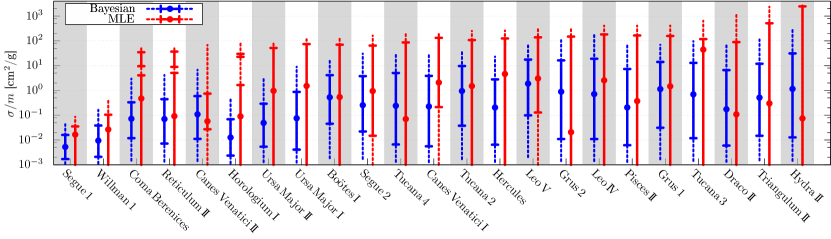
In Fig. 1, we show the fitting results of for . For the Bayesian analysis, we show the median of with and credible intervals. The figure shows that the posterior distributions of reach the lower limit of its prior distribution. Thus, no UFDs strongly favor non-zero self-interaction cross-section. This also means that the upper limit of strongly depends on the prior distribution in the Bayesian analysis.
For the MLE, we estimate the confidence intervals via and . We have checked that the estimated intervals by the MLE are consistent with the bootstrap Monte-Carlo simulation. The figure again shows that no UFDs favor non-zero cross-section. In particular, the fitting results for Segue 1 and Willman 1 are consistent with zero cross-section at C.L. and provide the upper-limit and , respectively.
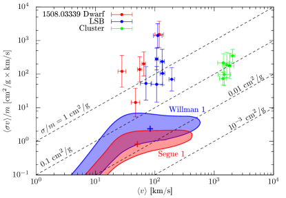
In Fig. 2, we show the estimation of with the MLE for Segue 1 and Willman 1, which correspond to two dimensional contours of . Compared with the favored SIDM cross-section in the previous study using the dwarf irregular galaxies Oh et al. (2011), the low surface brightness galaxies de Naray et al. (2008) (blue), and galaxy clusters Newman et al. (2013) (green) (see Ref. Kaplinghat et al. (2016) for details), the Segue 1 and Willman 1 place stringent upper limits.
V Conclusion
We investigated the SIDM by using the stellar kinematics of the 23 UFD galaxies with the phenomenological modeling of the SIDM halo profile. We found all the UFD galaxies are consistent with collisionless DM. In particular, Segue 1 and Willman 1 provide stringent constraints on the self-interacting cross-section: . As seen in Fig. 2, our result with the UFDs is in considerable tension with the DM self-interaction strength preferred by the dwarf irregular and the low surface brightness galaxies which are more affected by the baryonic feedback effects than the UFDs. In the present framework, it would not be easy to explain this discrepancy with the DM velocity dependent cross-section, as the typical velocities of the DM in the UFDs and those in the dwarf irregular galaxies are close with each other 333For a model which predicts the SIDM cross-section with an intricate velocity dependence, see e.g. Ref.Chu et al. (2019)..
It should be emphasized that our analysis is based on the simple steady-state modeling of the SIDM in Refs. Kaplinghat et al. (2016); Valli and Yu (2018). If some of the UFDs are in the core-collapse phase, for example, the simple model does not describe their halo profiles properly, which could invalidate the constraints obtained in this work. (See Ref. Correa (2020) for the study of the SIDM using the classical dSphs in which the core-collapse process is taken into account semi-analytically Balberg et al. (2002).) The estimation of the core-collapse time scale of the subhalo, however, may depend on subtle dynamics such as the tidal-stripping, and hence, needs further studies Vogelsberger et al. (2012); Rocha et al. (2013); Elbert et al. (2015); Nishikawa et al. (2020); Kummer et al. (2019); Robles et al. (2019); Sameie et al. (2020); Kahlhoefer et al. (2019).
Acknowledgements.
We thank H. Yu, M. Valli and S. Ando for helpful discussions. This work is supported by Grant-in-Aid for Scientific Research from the Ministry of Education, Culture, Sports, Science, and Technology (MEXT), Japan, 17H02878 (M.I. and S.S.), 18H05542 (M.I.) 18K13535, 19H04609, 20H01895 (S.S.) and 20H01895 (K.H.), and by World Premier International Research Center Initiative (WPI), MEXT, Japan. This work is also supported by the Advanced Leading Graduate Course for Photon Science (S.K.), the JSPS Research Fellowships for Young Scientists (S.K.) and International Graduate Program for Excellence in Earth-Space Science (Y.N.).References
- Vogelsberger et al. (2014a) M. Vogelsberger, S. Genel, V. Springel, P. Torrey, D. Sijacki, D. Xu, G. F. Snyder, S. Bird, D. Nelson, and L. Hernquist, Nature 509, 177 (2014a), arXiv:1405.1418 [astro-ph.CO] .
- Vogelsberger et al. (2014b) M. Vogelsberger, S. Genel, V. Springel, P. Torrey, D. Sijacki, D. Xu, G. F. Snyder, D. Nelson, and L. Hernquist, Mon. Not. Roy. Astron. Soc. 444, 1518 (2014b), arXiv:1405.2921 [astro-ph.CO] .
- Schaye et al. (2015) J. Schaye et al., Mon. Not. Roy. Astron. Soc. 446, 521 (2015), arXiv:1407.7040 [astro-ph.GA] .
- Springel et al. (2018) V. Springel et al., Mon. Not. Roy. Astron. Soc. 475, 676 (2018), arXiv:1707.03397 [astro-ph.GA] .
- Tulin and Yu (2018) S. Tulin and H.-B. Yu, Phys. Rept. 730, 1 (2018), arXiv:1705.02358 [hep-ph] .
- Bullock and Boylan-Kolchin (2017) J. S. Bullock and M. Boylan-Kolchin, Ann. Rev. Astron. Astrophys. 55, 343 (2017), arXiv:1707.04256 [astro-ph.CO] .
- McGaugh and de Blok (1998) S. S. McGaugh and W. J. G. de Blok, The Astrophysical Journal 499, 41–65 (1998).
- de Blok et al. (2001) W. J. G. de Blok, S. S. McGaugh, A. Bosma, and V. C. Rubin, The Astrophysical Journal 552, L23–L26 (2001).
- Oh et al. (2011) S.-H. Oh, W. J. G. de Blok, E. Brinks, F. Walter, and R. C. Kennicutt, The Astronomical Journal 141, 193 (2011).
- Read et al. (2017) J. Read, G. Iorio, O. Agertz, and F. Fraternali, Mon. Not. Roy. Astron. Soc. 467, 2019 (2017), arXiv:1607.03127 [astro-ph.GA] .
- Spergel and Steinhardt (2000) D. N. Spergel and P. J. Steinhardt, Physical Review Letters 84, 3760–3763 (2000).
- Vogelsberger et al. (2012) M. Vogelsberger, J. Zavala, and A. Loeb, Mon. Not. Roy. Astron. Soc. 423, 3740 (2012), arXiv:1201.5892 [astro-ph.CO] .
- Rocha et al. (2013) M. Rocha, A. H. Peter, J. S. Bullock, M. Kaplinghat, S. Garrison-Kimmel, J. Onorbe, and L. A. Moustakas, Mon. Not. Roy. Astron. Soc. 430, 81 (2013), arXiv:1208.3025 [astro-ph.CO] .
- Peter et al. (2013) A. H. Peter, M. Rocha, J. S. Bullock, and M. Kaplinghat, Mon. Not. Roy. Astron. Soc. 430, 105 (2013), arXiv:1208.3026 [astro-ph.CO] .
- Zavala et al. (2013) J. Zavala, M. Vogelsberger, and M. G. Walker, Mon. Not. Roy. Astron. Soc. 431, L20 (2013), arXiv:1211.6426 [astro-ph.CO] .
- Elbert et al. (2015) O. D. Elbert, J. S. Bullock, S. Garrison-Kimmel, M. Rocha, J. Oñorbe, and A. H. Peter, Mon. Not. Roy. Astron. Soc. 453, 29 (2015), arXiv:1412.1477 [astro-ph.GA] .
- Fry et al. (2015) A. B. Fry, F. Governato, A. Pontzen, T. Quinn, M. Tremmel, L. Anderson, H. Menon, A. Brooks, and J. Wadsley, Mon. Not. Roy. Astron. Soc. 452, 1468 (2015), arXiv:1501.00497 [astro-ph.CO] .
- Note (1) For high surface brightness galaxies, the inner halo may be cuspy in the SIDM model due to the gravitational potential from baryons Kaplinghat et al. (2014); Vogelsberger et al. (2014c); Kaplinghat et al. (2016); Kamada et al. (2017); Creasey et al. (2017); Elbert et al. (2018); Robertson et al. (2018); Ren et al. (2019). This behavior allows the SIDM model to solve the diversity problem Oman et al. (2015, 2016).
- Markevitch et al. (2004) M. Markevitch, A. H. Gonzalez, D. Clowe, A. Vikhlinin, W. Forman, C. Jones, S. Murray, and W. Tucker, The Astrophysical Journal 606, 819–824 (2004).
- Randall et al. (2008) S. W. Randall, M. Markevitch, D. Clowe, A. H. Gonzalez, and M. Bradač, The Astrophysical Journal 679, 1173–1180 (2008).
- Kahlhoefer et al. (2013) F. Kahlhoefer, K. Schmidt-Hoberg, M. T. Frandsen, and S. Sarkar, Monthly Notices of the Royal Astronomical Society 437, 2865–2881 (2013).
- Harvey et al. (2015) D. Harvey, R. Massey, T. Kitching, A. Taylor, and E. Tittley, Science 347, 1462–1465 (2015).
- Robertson et al. (2016) A. Robertson, R. Massey, and V. Eke, Monthly Notices of the Royal Astronomical Society 465, 569–587 (2016).
- Wittman et al. (2018) D. Wittman, N. Golovich, and W. A. Dawson, The Astrophysical Journal 869, 104 (2018).
- Harvey et al. (2019) D. Harvey, A. Robertson, R. Massey, and I. G. McCarthy, Monthly Notices of the Royal Astronomical Society 488, 1572–1579 (2019).
- Bondarenko et al. (2020) K. Bondarenko, A. Sokolenko, A. Boyarsky, A. Robertson, D. Harvey, and Y. Revaz, (2020), arXiv:2006.06623 [astro-ph.CO] .
- Sagunski et al. (2020) L. Sagunski, S. Gad-Nasr, B. Colquhoun, A. Robertson, and S. Tulin, (2020), arXiv:2006.12515 [astro-ph.CO] .
- Read and Gilmore (2005) J. I. Read and G. Gilmore, Mon. Not. Roy. Astron. Soc. 356, 107 (2005), arXiv:astro-ph/0409565 .
- Mashchenko et al. (2008) S. Mashchenko, J. Wadsley, and H. Couchman, Science 319, 174 (2008), arXiv:0711.4803 [astro-ph] .
- Pontzen and Governato (2012) A. Pontzen and F. Governato, Mon. Not. Roy. Astron. Soc. 421, 3464 (2012), arXiv:1106.0499 [astro-ph.CO] .
- Oñorbe et al. (2015) J. Oñorbe, M. Boylan-Kolchin, J. S. Bullock, P. F. Hopkins, D. s. Kerˇes, C.-A. Faucher-Giguère, E. Quataert, and N. Murray, Mon. Not. Roy. Astron. Soc. 454, 2092 (2015), arXiv:1502.02036 [astro-ph.GA] .
- Tollet et al. (2016) E. Tollet et al., Mon. Not. Roy. Astron. Soc. 456, 3542 (2016), [Erratum: Mon.Not.Roy.Astron.Soc. 487, 1764 (2019)], arXiv:1507.03590 [astro-ph.GA] .
- Hayashi et al. (2020) K. Hayashi, M. Chiba, and T. Ishiyama, (2020), arXiv:2007.13780 [astro-ph.GA] .
- Kaplinghat et al. (2016) M. Kaplinghat, S. Tulin, and H.-B. Yu, Physical Review Letters 116 (2016), 10.1103/physrevlett.116.041302.
- Valli and Yu (2018) M. Valli and H.-B. Yu, Nature Astron. 2, 907 (2018), arXiv:1711.03502 [astro-ph.GA] .
- Binney and Tremaine (2008) J. Binney and S. Tremaine, Galactic Dynamics: Second Edition (2008).
- Baes and Van Hese (2007) M. Baes and E. Van Hese, Astron. Astrophys. 471, 419 (2007), arXiv:0705.4109 [astro-ph] .
- Plummer (1911) H. C. Plummer, Mon. Not. Roy. Astron. Soc. 71, 460 (1911).
- Note (2) Here, the mass density and the pressure of DM are related by . This corresponds to the Maxwell-Boltzmann velocity distribution, . We do not truncate the distribution by the escape velocity. In this case, the mean relative DM velocity is given by, .
- Navarro et al. (1997) J. F. Navarro, C. S. Frenk, and S. D. White, Astrophys. J. 490, 493 (1997), arXiv:astro-ph/9611107 .
- Vogelsberger et al. (2016) M. Vogelsberger, J. Zavala, F.-Y. Cyr-Racine, C. Pfrommer, T. Bringmann, and K. Sigurdson, Mon. Not. Roy. Astron. Soc. 460, 1399 (2016), arXiv:1512.05349 [astro-ph.CO] .
- Boylan-Kolchin et al. (2011) M. Boylan-Kolchin, J. S. Bullock, and M. Kaplinghat, Mon. Not. Roy. Astron. Soc. 415, L40 (2011), arXiv:1103.0007 [astro-ph.CO] .
- Boylan-Kolchin et al. (2012) M. Boylan-Kolchin, J. S. Bullock, and M. Kaplinghat, Mon. Not. Roy. Astron. Soc. 422, 1203 (2012), arXiv:1111.2048 [astro-ph.CO] .
- Moliné et al. (2017) A. Moliné, M. A. Sánchez-Conde, S. Palomares-Ruiz, and F. Prada, Mon. Not. Roy. Astron. Soc. 466, 4974 (2017), arXiv:1603.04057 [astro-ph.CO] .
- Ishiyama and Ando (2020) T. Ishiyama and S. Ando, Mon. Not. Roy. Astron. Soc. 492, 3662 (2020), arXiv:1907.03642 [astro-ph.CO] .
- Wang et al. (2020) W. Wang, J. Han, M. Cautun, Z. Li, and M. N. Ishigaki, Sci. China Phys. Mech. Astron. 63, 109801 (2020), arXiv:1912.02599 [astro-ph.GA] .
- Martin et al. (2008) N. F. Martin, J. T. A. de Jong, and H.-W. Rix, Astrophys. J. 684, 1075 (2008), arXiv:0805.2945 [astro-ph] .
- Belokurov et al. (2009) V. Belokurov, M. Walker, N. Evans, G. Gilmore, M. Irwin, M. Mateo, L. Mayer, E. Olszewski, J. Bechtold, and T. Pickering, Mon. Not. Roy. Astron. Soc. 397, 1748 (2009), arXiv:0903.0818 [astro-ph.GA] .
- Koposov et al. (2015) S. E. Koposov, V. Belokurov, G. Torrealba, and N. W. Evans, Astrophys. J. 805, 130 (2015), arXiv:1503.02079 [astro-ph.GA] .
- Martin et al. (2015) N. F. Martin et al., Astrophys. J. Lett. 804, L5 (2015), arXiv:1503.06216 [astro-ph.GA] .
- Sand et al. (2012) D. Sand, J. Strader, B. Willman, D. Zaritsky, B. McLeod, N. Caldwell, A. Seth, and E. Olszewski, Astrophys. J. 756, 79 (2012), arXiv:1111.6608 [astro-ph.CO] .
- Drlica-Wagner et al. (2015) A. Drlica-Wagner et al. (DES), Astrophys. J. 813, 109 (2015), arXiv:1508.03622 [astro-ph.GA] .
- Bechtol et al. (2015) K. Bechtol et al. (DES), Astrophys. J. 807, 50 (2015), arXiv:1503.02584 [astro-ph.GA] .
- Muñoz et al. (2018) R. R. Muñoz et al., Astrophys. J. 860, 66 (2018), arXiv:1806.06891 [astro-ph.GA] .
- Simon et al. (2011) J. D. Simon et al., Astrophys. J. 733, 46 (2011), arXiv:1007.4198 [astro-ph.GA] .
- Kirby et al. (2013) E. N. Kirby, M. Boylan-Kolchin, J. G. Cohen, M. Geha, J. S. Bullock, and M. Kaplinghat, Astrophys. J. 770, 16 (2013), arXiv:1304.6080 [astro-ph.CO] .
- Koposov et al. (2011) S. E. Koposov et al., Astrophys. J. 736, 146 (2011), arXiv:1105.4102 [astro-ph.GA] .
- Simon and Geha (2007) J. D. Simon and M. Geha, Astrophys. J. 670, 313 (2007), arXiv:0706.0516 [astro-ph] .
- Simon et al. (2015) J. Simon et al. (DES), Astrophys. J. 808, 95 (2015), arXiv:1504.02889 [astro-ph.GA] .
- Martin et al. (2016) N. F. Martin et al., Mon. Not. Roy. Astron. Soc. 458, L59 (2016), arXiv:1510.01326 [astro-ph.GA] .
- Kirby et al. (2017) E. N. Kirby, J. G. Cohen, J. D. Simon, P. Guhathakurta, A. O. Thygesen, and G. E. Duggan, Astrophys. J. 838, 83 (2017), arXiv:1703.02978 [astro-ph.GA] .
- Kirby et al. (2015) E. N. Kirby, J. D. Simon, and J. G. Cohen, Astrophys. J. 810, 56 (2015), arXiv:1506.01021 [astro-ph.GA] .
- Walker et al. (2016) M. G. Walker et al., Astrophys. J. 819, 53 (2016), arXiv:1511.06296 [astro-ph.GA] .
- Simon et al. (2020) J. Simon et al. (DES), Astrophys. J. 892, 137 (2020), arXiv:1911.08493 [astro-ph.GA] .
- Koposov et al. (2015) S. E. Koposov et al., Astrophys. J. 811, 62 (2015), arXiv:1504.07916 [astro-ph.GA] .
- Simon et al. (2017) J. Simon et al. (DES), Astrophys. J. 838, 11 (2017), arXiv:1610.05301 [astro-ph.GA] .
- Willman et al. (2011) B. Willman, M. Geha, J. Strader, L. E. Strigari, J. D. Simon, E. Kirby, and A. Warres, Astron. J. 142, 128 (2011), arXiv:1007.3499 [astro-ph.GA] .
- Goodman and Weare (2010) J. Goodman and J. Weare, Communications in Applied Mathematics and Computational Science 5, 65 (2010).
- de Naray et al. (2008) R. K. de Naray, S. S. McGaugh, and W. J. G. de Blok, The Astrophysical Journal 676, 920–943 (2008).
- Newman et al. (2013) A. B. Newman, T. Treu, R. S. Ellis, and D. J. Sand, The Astrophysical Journal 765, 25 (2013).
- Note (3) For a model which predicts the SIDM cross-section with an intricate velocity dependence, see e.g. Ref.Chu et al. (2019).
- Correa (2020) C. A. Correa, (2020), arXiv:2007.02958 [astro-ph.GA] .
- Balberg et al. (2002) S. Balberg, S. L. Shapiro, and S. Inagaki, Astrophys. J. 568, 475 (2002), arXiv:astro-ph/0110561 .
- Nishikawa et al. (2020) H. Nishikawa, K. K. Boddy, and M. Kaplinghat, Phys. Rev. D 101, 063009 (2020), arXiv:1901.00499 [astro-ph.GA] .
- Kummer et al. (2019) J. Kummer, M. Brüggen, K. Dolag, F. Kahlhoefer, and K. Schmidt-Hoberg, Mon. Not. Roy. Astron. Soc. 487, 354 (2019), arXiv:1902.02330 [astro-ph.CO] .
- Robles et al. (2019) V. H. Robles, T. Kelley, J. S. Bullock, and M. Kaplinghat, Mon. Not. Roy. Astron. Soc. 490, 2117 (2019), arXiv:1903.01469 [astro-ph.GA] .
- Sameie et al. (2020) O. Sameie, H.-B. Yu, L. V. Sales, M. Vogelsberger, and J. Zavala, Phys. Rev. Lett. 124, 141102 (2020), arXiv:1904.07872 [astro-ph.GA] .
- Kahlhoefer et al. (2019) F. Kahlhoefer, M. Kaplinghat, T. R. Slatyer, and C.-L. Wu, JCAP 12, 010 (2019), arXiv:1904.10539 [astro-ph.GA] .
- Kaplinghat et al. (2014) M. Kaplinghat, R. E. Keeley, T. Linden, and H.-B. Yu, Physical Review Letters 113 (2014), 10.1103/physrevlett.113.021302.
- Vogelsberger et al. (2014c) M. Vogelsberger, J. Zavala, C. Simpson, and A. Jenkins, Monthly Notices of the Royal Astronomical Society 444, 3684–3698 (2014c).
- Kamada et al. (2017) A. Kamada, M. Kaplinghat, A. B. Pace, and H.-B. Yu, Physical Review Letters 119 (2017), 10.1103/physrevlett.119.111102.
- Creasey et al. (2017) P. Creasey, O. Sameie, L. V. Sales, H.-B. Yu, M. Vogelsberger, and J. Zavala, Monthly Notices of the Royal Astronomical Society 468, 2283–2295 (2017).
- Elbert et al. (2018) O. D. Elbert, J. S. Bullock, M. Kaplinghat, S. Garrison-Kimmel, A. S. Graus, and M. Rocha, The Astrophysical Journal 853, 109 (2018).
- Robertson et al. (2018) A. Robertson, R. Massey, V. Eke, S. Tulin, H.-B. Yu, Y. Bahé, D. J. Barnes, R. G. Bower, R. A. Crain, C. Dalla Vecchia, and et al., Monthly Notices of the Royal Astronomical Society: Letters 476, L20–L24 (2018).
- Ren et al. (2019) T. Ren, A. Kwa, M. Kaplinghat, and H.-B. Yu, Physical Review X 9 (2019), 10.1103/physrevx.9.031020.
- Oman et al. (2015) K. A. Oman, J. F. Navarro, A. Fattahi, C. S. Frenk, T. Sawala, S. D. M. White, R. Bower, R. A. Crain, M. Furlong, M. Schaller, and et al., Monthly Notices of the Royal Astronomical Society 452, 3650–3665 (2015).
- Oman et al. (2016) K. A. Oman, J. F. Navarro, L. V. Sales, A. Fattahi, C. S. Frenk, T. Sawala, M. Schaller, and S. D. M. White, Monthly Notices of the Royal Astronomical Society 460, 3610–3623 (2016).
- Chu et al. (2019) X. Chu, C. Garcia-Cely, and H. Murayama, Phys. Rev. Lett. 122, 071103 (2019), arXiv:1810.04709 [hep-ph] .