Ab initio framework for systems with helical symmetry: theory, numerical implementation and applications to torsional deformations in nanostructures

Abstract

We formulate and implement Helical Density Functional Theory (Helical DFT) — a self-consistent first principles simulation method for nanostructures with helical symmetries. Such materials are well represented in all of nanotechnology, chemistry and biology, and prominent examples include nanotubes, nanosprings, nanowires, miscellaneous chiral structures and important proteins. The overwhelming preponderance of such helical structures in all of science and engineering and the likelihood of these systems being associated with exotic materials properties, provides the motivation to develop systematic and predictive tools for their study.

Following this line of thought, we develop a mathematical and computational framework in this contribution, that allows helical structures to be studied ab initio, using Kohn-Sham theory. We first show that the electronic states in helical structures can be characterized by means of special solutions to the single electron problem called helical Bloch waves. We rigorously demonstrate the existence and completeness of such solutions, and then describe how they can be used to reduce the Kohn-Sham Density Functional Theory (KS-DFT) equations for helical structures to a suitable fundamental domain. Next, we develop a symmetry-adapted finite-difference strategy in helical coordinates to discretize the governing equations, and obtain a working realization of our proposed approach. We verify the accuracy and convergence properties of our numerical implementation through examples. Finally, we employ Helical DFT to study the properties of zigzag and chiral single wall black phosphorus (i.e., phosphorene) nanotubes. Specifically, we use our simulations to evaluate the torsional stiffness of a zigzag nanotube ab initio. Additionally, we observe an insulator-to-metal-like transition in the electronic properties of this nanotube as it is subjected to twisting. We also find that a similar transition can be effected in chiral phosphorene nanotubes by means of axial strains. The strong dependence of the band gap of these materials on various modes of strain suggests their possible use as nanomaterials with tunable electronic and transport properties. Notably, self-consistent ab initio simulations of this nature are unprecedented and well outside the scope of any other systematic first principles method in existence. We end with a discussion on various future avenues and applications.

1 Introduction

The discovery and characterization of novel nanomaterials and nanostructures constitutes one of the principal areas of scientific research today [1, 2]. Such materials and structures hold the promise of unlocking remarkable and unprecedented material properties that are otherwise unavailable in the bulk phase (i.e., crystalline materials). In recent years, the discovery of novel nanostructures has garnered much attention and acclaim [3, 4], and the unusual properties of these new materials have led to ground breaking applications in almost every branch of science and engineering [5, 6].

Nanostructures appear in various morphologies (including fullerenes, nanotubes, nanoclusters and two-dimensional materials), and are usually associated with non-periodic symmetries. The mathematical framework for classifying nanostructures [7, 9, 10] shows that a vast class of these materials can be described as being helical, i.e., their spatial atomic arrangement possesses helical symmetries. Helical structures include important technological materials such as nanotubes (of any chirality), nanoribbons, nanowires and nanosprings; miscellaneous chiral structures encountered in chemistry; and examples from biology, including tail sheaths of viruses and many common proteins [7, 11]. Figure 1a shows instances of helical structures that have been actively investigated in the literature.

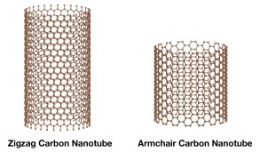
(a) Nanotubes of different chirality.

Figure 1: Examples of helical structures from nanotechnology and biology. Images of the Amyloid protein were obtained courtesy of The Protein Data Bank [12, 13, 14].

 

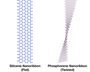
(b) Nanoribbons of different 2D materials.

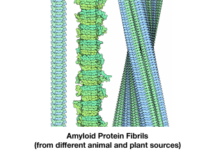
(c) Molecules of biological origin.

Helical structures have been conjectured to be a fertile source of novel materials with unusual and attractive properties [7]. This is due to the fact that atoms in such structures find themselves in locally similar environments [7]. Coupled with the quasi-one-dimensional nature of these systems, as well as the presence of symmetries in the underlying governing equations, this makes it likely that collective or correlated electronic effects (such as those leading to ferromagnetism, ferroelectricity and superconductivity) can emerge in these materials [15]. On the other hand, helical structures are also inherently chiral and can therefore serve as natural examples of materials systems in which certain forms of symmetry breaking in the governing equations can lead to unconventional transport phenomena [16, 17, 18, 19].

Given the relative abundance of helical nanostructures in existing materials, their likelihood of being associated with hitherto undiscovered forms of matter displaying exotic materials properties, and their overall scientific and technological importance, there appears to be a pressing need for reliable and efficient computational tools for studying such systems. The broad goal of the present contribution is to take important foundational steps in addressing the above scientific issue. Specifically, we present here the mathematical formulation and numerical implementation of a novel computational method called Helical DFT, that can simulate helical structures ab initio. We also obtain a practical working realization of this (density functional theory based) self-consistent first principles technique, and illustrate some of its capabilities through the study of an emergent nanotube material with interesting properties.

To put our work into perspective, we remark that the use of first principles (i.e., quantum mechanical) techniques to design and study materials is a very active area of scientific endeavor today, and it forms the bulk of computational materials science research [20, 21, 22, 23, 24]. Among the wide array of first principles methods available, Kohn-Sham Density Functional Theory (KS-DFT) [25] enjoys widespread usage since it offers a good balance between computational cost and physical accuracy as compared to other techniques [26]. The pseudopotential plane-wave method, also called Plane-wave DFT, is the most widely used implementation of Kohn-Sham theory [27, 28, 29, 30], and it involves expanding the unknowns into linear combinations of plane-waves. Since plane-waves are naturally associated with periodic symmetries (they are in fact eigenfunctions of translational symmetry operators), Plane-wave DFT is ideally suited for studying bulk (i.e. periodic or crystalline) systems, and is often found to be fundamentally inadequate for studying systems with non-periodic symmetries. In particular, using a Plane-wave DFT code for studying a helical structure such as a chiral nanotube can require the use of large periodic unit cells often containing many hundreds (or even thousands) of atoms. In contrast, a computational method which is faithful to the underlying helical symmetry of such a structure would require a small helical unit cell, containing far fewer number of atoms. Since ground state electronic structure calculations using density functional theory (DFT) scale as the cube of the number of atoms in the unit cell, while excited state calculations scale as the fourth power, the difference in simulation run times for such calculations, in these two scenarios (i.e., the correct use of helical symmetry vs. incorrect use of periodic symmetry) can be drastically different in practice.

The above considerations form our point of departure from a conventional formulation and implementation of KS-DFT, to one that is adapted for helical systems. In order to formulate the equations of KS-DFT for a helical unit cell, an appropriate version of the Bloch Theorem [38, 39] is required. We establish this result rigorously in this work, and use it to set up an electronic band theory for helical structures. Subsequently, we develop the notion of helical Bloch states, and use their properties to derive of the equations of KS-DFT, as they apply to helical systems. A key component in our mathematical treatment is the definition and use of a helical Bloch-Floquet transform to perform a block-diagonalization of the Hamiltonian in the sense of direct integrals. Our use of rigorous mathematical arguments and appropriate mathematical tools is one of the highlights of our framework, and it allows the governing equations to be obtained systematically, and without recourse to an excessive amount of intuition. As far as we are aware, our work is the first in presenting such a derivation, and also in expressing the detailed form of the equations of Kohn-Sham theory for helical structures. The final form of the equations are such that they are readily suited for implementation within systematically convergent electronic structure methods such as those based on finite differences [31, 32, 33, 34], finite elements [35, 36, 37] or spectral basis functions [8, 45, 46]. We choose a symmetry adapted finite difference method in helical coordinates for discretizing the governing equations in this work, and set up a computational framework for numerically solving the discretized equations in a self-consistent manner. This gives us a working realization of an ab initio computational tool — called Helical DFT — that can be used to perform predictive simulations of helical systems in a systematic and efficient manner. It can therefore aid in the discovery, synthesis and characterization of helical structures. Subsequently, the remainder of this work focuses on illustrating various numerical and application oriented aspects of this novel computational tool through examples based on nanotube systems. To the best of our knowledge, Helical DFT is the first computational method for helical systems that is based on first principles, and one that also behaves systematically with respect to convergence properties. This, among other reasons, is made possible by our use of the aforementioned helical coordinate system. To the best of our knowledge, this has not been employed in electronic structure calculations before.

While the study of helical structures has much scientific and technological merit in of itself, the development of a computational method for studying such systems also brings with it the added benefit of being able to simulate the behavior of nanomaterials under torsional deformations. As explained in [7, 40], homogeneous deformation modes are commensurate with periodic symmetries (i.e., applying a homogeneous deformation to a periodic structure results in another periodic structure), while certain inhomogeneous deformation modes can be associated with non-periodic symmetries. An attempt to study such inhomogeneous deformations while using a periodic method is likely to involve various uncontrolled approximations, complications and computational inefficiencies [47, 48]. This issue appears to have been recognized for some time in the nanomechanics and materials literature, leading to a considerable body of work centered around suggestions presented in [7], whereby pure bending deformations in atomistic systems are simulated using cyclic symmetries, while helical symmetries are used to simulate torsion [49, 50, 51, 52, 53, 54, 55, 56, 57, 58]. A persistent issue with the simulations in these studies however, is that they have all been carried out using interatomic potentials or tight binding methods. Due to the well known deficiencies of these techniques in simulating real materials [59, 60, 61, 62, 48], true first principles simulation methods that behave systematically, and also take into account cyclic and/or helical symmetries have been deemed highly desirable [58, 7, 8]. There has been recent progress on this very issue with regard to cyclic symmetries [40, 63], and the resulting computational methods have been used to study the bending behavior of nanoribbons and sheets of two dimensional materials ab initio. In this sense, the current contribution follows up on this line of work by making a first principles simulation framework for torsional deformations available. Consequently, through the use of this framework, we are able to extract the behavior of nanotubes of black phosphorus (i.e., phosphorene nanotubes) and study their mechanical and electronic response as they are subjected to twisting. The coupling of these responses leads to some interesting electronic transitions in this material that is likely to make it an attractive candidate for sensing, modulation and actuation applications.

The rest of this work is organized as follows. Section 2 establishes the mathematical framework for a systematic formulation of the governing equations, and also derives the relevant expressions explicitly. Section 3 discusses formulation of a numerical scheme based on finite differences in helical coordinates, and Section 4 presents simulation studies. Section 5 summarizes the work and suggests avenues for future research. The appendices contain additional information and discussions on mathematical tools and results that allow for this work to be self-contained.

2 Formulation

In this section, we describe the key aspects of Helical DFT. We begin with a formal discussion of helical groups and helical structures in Section 2.1, and then discuss Kohn-Sham DFT, as it applies to such systems in Section 2.2. The atomic unit system with $m_{\text{e}}=1,e=1,\hbar=1,\frac{1}{4\pi\epsilon_{0}}=1$, is chosen for the rest of the work, unless otherwise mentioned.

2.1 Helical symmetry groups, fundamental domains and helical structures

A helical structure (i.e. a structure with helical symmetries) can be defined through the action of a helical group on a set of non-degenerate points in space. This definition makes it necessary for us to make the notion of a helical group precise. Following standard practice in the literature [9, 7, 49, 10, 70, 71, 8], we introduce helical groups as subgroups of the Euclidean group in three dimensions. This requires us to introduce some relevant notation and basic rules regarding operations with isometries, as we now do.

2.1.1 Helical symmetry groups

Let ${\bf e}_{1},{\bf e}_{2},{\bf e}_{3}$ denote the standard orthonormal basis of $\mathbb{R}^{3}$ and let $(x_{1},x_{2},x_{3})$ denote the Cartesian coordinates of a generic point ${\bf x}\in\mathbb{R}^{3}$. An isometry (or rigid body motion) in $\mathbb{R}^{3}$ will be denoted using the notation $\Upsilon=({\bf R}|{\bf c})$, with ${\bf R}\in\text{SO}(3)$ denoting the rotation part of the rigid body motion, and ${\bf c}\in\mathbb{R}^{3}$ denoting the translation part. The action of $\Upsilon:\mathbb{R}^{3}\to\mathbb{R}^{3}$ on a point ${\bf x}\in\mathbb{R}^{3}$ is written as $\Upsilon\circ{\bf x}={\bf R}{\bf x}+{\bf c}$. Given a collection of points $S\subset\mathbb{R}^{3}$, we will use the notation $\Upsilon\circ S$ to denote the action of the isometry on each of the points in $S$, i.e.,

$$\Upsilon\circ S:=\bigcup_{{\bf x}\in S}\Upsilon\circ{\bf x}\,.$$ (1)

There is a natural multiplicative operation associated with isometries (denoted as $\bullet$ here) that arises as a composition of their maps. Specifically, given isometries $\Upsilon_{1}=({\bf R}_{1}|{\bf c}_{1}),\Upsilon_{2}=({\bf R}_{2}|{\bf c}_{2})$, we may define a third isometry $\Upsilon_{3}=\Upsilon_{1}\bullet\Upsilon_{2}$ such that $\Upsilon_{3}\circ{\bf x}=(\Upsilon_{1}\bullet\Upsilon_{2})\circ{\bf x}:=\Upsilon_{1}\circ(\Upsilon_{2}\circ{\bf x})$. It follows that $\Upsilon_{3}=({\bf R}_{1}{\bf R}_{2}|{\bf R}_{1}{\bf c}_{2}+{\bf c}_{1})$, and that in general the operation $\bullet$ is not commutative (due to non-commutativity of finite rotations about arbitrary axes). The $\bullet$ operation also allows the definition of whole number powers of $\Upsilon$, i.e., for $n=1,2,\ldots$, we may define $\Upsilon^{n}:=\Upsilon\bullet\Upsilon\bullet\Upsilon\ldots(n\;\text{times})$. It is then easy to check that $\Upsilon^{n}$ admits the expression $\displaystyle\Upsilon^{n}=\big{(}{\bf R}^{n}\big{|}(\sum_{j=0}^{n-1}{\bf R}^{j})\,{\bf c}\big{)}$, where the notation ${\bf R}^{0}$ is used to denote the identity matrix.

The identity isometry leaves every ${\bf x}\in\mathbb{R}^{3}$ invariant and can be written as $({\bf I}|\textbf{0})$, with ${\bf I}$ denoting the identity matrix and 0 denoting the null vector in $\mathbb{R}^{3}$. Given the isometry $\Upsilon=({\bf R}|{\bf c})$, we can form the isometry $\Upsilon^{\prime}=({\bf R}^{-1}|-{\bf R}^{-1}{\bf c})$, which satisfies $\Upsilon\bullet\Upsilon^{\prime}=\Upsilon^{\prime}\bullet\Upsilon=({\bf I}|\textbf{0})$. Hence, we will denote $\Upsilon^{\prime}$ as $\Upsilon^{-1}$ — i.e., the inverse isometry to $\Upsilon$. The set of all isometries so defined, i.e., $\mathcal{E}=\{\Upsilon=({\bf R}|{\bf c}):{\bf R}\in\text{SO}(3),{\bf c}\in\mathbb{R}^{3}\}$, together with the operation $\bullet$ and the inverse element defined above, form a group [72].

Let $\alpha$ and $\tau$ be real numbers such that $0\leq\alpha<1$ and $\tau>0$, and let ${\bf R}_{2\pi\alpha}$ denote a rotation around axis ${\bf e}_{3}$ by angle $2\pi\alpha$. Then, the rigid body motion $\Upsilon_{\mathsf{h}}=({\bf R}_{2\pi\alpha}|\tau{\bf e}_{3})$ will be called a helical isometry about axis ${\bf e}_{3}$. The action of $\Upsilon_{\mathsf{h}}$ on a point ${\bf x}\in\mathbb{R}^{3}$ is to rotate it by angle $2\pi\alpha$ about axis ${\bf e}_{3}$, while also translating it by $\tau$ along the same axis. Furthermore, applying the formulae for the powers of isometries and their inverses shown above, we see that for $m=1,2,\ldots$, $\Upsilon_{\mathsf{h}}^{m}=({\bf R}_{2\pi m\alpha}|m\tau{\bf e}_{3})$ and $\Upsilon_{\mathsf{h}}^{-1}=({\bf R}_{-2\pi\alpha}|-\tau{\bf e}_{3})$. Combining these, we may define $\Upsilon_{\mathsf{h}}^{m}$ for any $m\in\mathbb{Z}$ as $\Upsilon_{\mathsf{h}}^{m}=({\bf R}_{2\pi m\alpha}|m\tau{\bf e}_{3})$, with the $m=0$ case automatically resulting in the identity isometry $({\bf I}|\textbf{0})$. We may therefore state:

Proposition 2.1 (Helical group generated by a single element).

The set of isometries

$${\cal G}_{1}=\big{\{}\Upsilon_{\mathsf{h}}^{m}=({\bf R}_{2\pi m\alpha}|m\tau{\bf e}_{3}):m\in\mathbb{Z}\big{\}}\,,$$ (2)

forms a discrete group under the operation $\bullet$.

Additionally, let $\mathfrak{N}\in\mathbb{N}$, let $\displaystyle{\Theta}=\frac{2\pi}{\mathfrak{N}}$ and for $n=0,1,\ldots,\mathfrak{N}-1$, let ${\bf R}_{n\Theta}$ denote a rotation around axis ${\bf e}_{3}$ by angle $n\Theta$. Then the set of isometries endowed with the operation $\bullet$

$$\mathfrak{C}=\big{\{}\Upsilon_{\mathsf{c}}^{n}=({\bf R}_{n\Theta}|\textbf{0}):n=0,1,\ldots,\mathfrak{N}-1\big{\}}\,,$$ (3)

forms a cyclic group [40] of order $\mathfrak{N}$. Note that since the rotational parts of the isometries in group ${\cal G}_{1}$ and $\mathfrak{C}$ all share ${\bf e}_{3}$ as the common axis of rotation, the elements of ${\cal G}_{1}$ and $\mathfrak{C}$ commute (i.e., for any $\Upsilon_{\mathsf{h}}^{m}\in{\cal G}_{1}$ and $\Upsilon_{\mathsf{c}}^{n}\in\mathfrak{C}$, $\Upsilon_{\mathsf{c}}^{n}\bullet\Upsilon_{\mathsf{h}}^{m}=\Upsilon_{\mathsf{h}}^{m}\bullet\Upsilon_{\mathsf{c}}^{n}$ holds.) . We may now consider the direct product of the groups ${\cal G}_{1}$ and $\mathfrak{C}$ defined above to obtain a new helical group:

Proposition 2.2 (Helical group generated by two elements).

The set of isometries

$${\cal G}_{2}=\big{\{}\Upsilon_{\mathsf{h}}^{m}\bullet\Upsilon_{\mathsf{c}}^{n}=({\bf R}_{2\pi m\alpha+n\Theta}|m\tau{\bf e}_{3}):m\in\mathbb{Z};n=0,1,\ldots,\mathfrak{N}-1\big{\}}\,,$$ (4)

forms a discrete group under the operation $\bullet$.

Since ${\cal G}_{1}$ and $\mathfrak{C}$ are generated by single elements, they are Abelian groups. Furthermore, since ${\cal G}_{2}$ is generated by two elements (i.e., the generators of ${\cal G}_{1}$ and $\mathfrak{C}$) which commute among themselves, it is an Abelian group as well.

The action of the groups ${\cal G}_{1}$ and ${\cal G}_{2}$ on points in space are easily described using cylindrical coordinates: if ${\bf x}\in\mathbb{R}^{3}$ is point with cylindrical coordinates $(r,\vartheta,z)$, then the action of the group element $\Upsilon_{h}^{m}\in{\cal G}_{1}$ is to send it to a point with cylindrical coordinates $(r,\vartheta+2\pi m\alpha,z+m\tau)$, while the action of $\Upsilon_{h}^{m}\bullet\Upsilon_{c}^{n}\in{\cal G}_{2}$ is to send it to the point with cylindrical coordinates $(r,\vartheta+2\pi m\alpha+n\Theta,z+m\tau)$. In what follows, we will use the notation $\widetilde{\Upsilon}$ to denote a generic isometry from ${\cal G}_{1}$ or ${\cal G}_{2}$.

2.1.2 Fundamental domains

Given a point ${\bf x}\in\mathbb{R}^{3}$, and a group of isometries ${\cal G}$ (which could be the helical groups ${\cal G}_{1}$ or ${\cal G}_{2}$ described above, for instance), the orbit of ${\bf x}$ under the group is the set

$${\cal G}\circ{\bf x}:=\{\widetilde{\Upsilon}\circ{\bf x}:\widetilde{\Upsilon}\in{\cal G}\}\,.$$ (5)

Given a collection of points $S\subset\mathbb{R}^{3}$ and a group of isometries ${\cal G}$, we will use the notation ${\cal G}\circ S$ to denote the orbits of each of the points in $S$ under the group:

$${\cal G}\circ S:=\bigcup_{{\bf x}\in S}{\cal G}\circ{\bf x}\;\;\bigg{(}=\bigcup_{\widetilde{\Upsilon}\in{\cal G}}\!\widetilde{\Upsilon}\circ S=\bigcup_{\begin{subarray}{c}\widetilde{\Upsilon}\in{\cal G},\\ {\bf x}\in S\end{subarray}}\!\!\widetilde{\Upsilon}\circ{\bf x}\bigg{)}\,.$$ (6)

Let ${\cal O}\subset\mathbb{R}^{3}$ be a domain with regular boundary that is invariant under a given helical group ${\cal G}$, i.e., ${\cal G}\circ{\cal O}={\cal O}$. The symmetry cell or fundamental domain of ${\cal G}$ in ${\cal O}$ is a set $D\subset{\cal O}$ such that:

$$\bigcup_{\widetilde{\Upsilon}\in{\cal G}}\!\widetilde{\Upsilon}\circ D={\cal O}\,,$$ (7)

and for $\widetilde{\Upsilon}_{1},\widetilde{\Upsilon}_{2}\in{\cal G}$:

$$(\widetilde{\Upsilon}_{1}\circ D)\,\bigcap\,(\widetilde{\Upsilon}_{2}\circ D)=\,\text{a set of Lebesgue measure}\;0\;\text{for}\;\widetilde{\Upsilon}_{1}\neq\widetilde{\Upsilon}_{2}.$$ (8)

To see concrete examples of the sets ${\cal O}$ and ${D}$, let $\mathscr{D}_{R}$ denote an open disk of radius $R$ on the ${\bf e}_{1},{\bf e}_{2}$ plane, i.e.,

$$\mathscr{D}_{R}=\{{\bf p}\in\mathbb{R}^{2}:\lVert{\bf p}\rVert_{\mathbb{R}^{2}}<R\}\,,$$ (9)

and let ${\cal C}$ denote the infinite cylinder obtained by translating $\mathscr{D}_{R}$ along ${\bf e}_{3}$, i.e.:

$${\cal C}=\mathscr{D}_{R}\times\{x_{3}\,{\bf e}_{3}:x_{3}\in\mathbb{R}\}\,.$$ (10)

Then, the cylinder ${\cal C}$ has all the properties required of the domain ${\cal O}$. Furthermore, we observe that the finite cylinder ${\cal D}_{{\cal G}_{1}}=\mathscr{D}_{R}\times\{x_{3}\,{\bf e}_{3}:0\leq x_{3}<\tau\}$ serves as the fundamental domain of ${\cal G}_{1}$ in ${\cal C}$. Finally, the sector with slanted walls, described in cylindrical coordinates as:

$${\cal D}_{{\cal G}_{2}}=\big{\{}(r,\vartheta,z):0\leq r<R,\frac{2\pi\alpha z}{\tau}\leq\vartheta<\frac{2\pi}{\mathfrak{N}}+\frac{2\pi\alpha z}{\tau},0\leq z<\tau\big{\}}\,,$$ (11)

serves as the fundamental domain of ${\cal G}_{2}$ in ${\cal C}$.

2.1.3 Helical Structures

A helical structure i.e., an atomic/molecular structure with helical symmetries is simply the orbit of a set of non-degenerate points under the action of one of the helical groups ${\cal G}_{1}$ or ${\cal G}_{2}$. More precisely, let ${\cal P}_{{\cal G}_{1}}\subset{\cal D}_{{\cal G}_{1}}$ (or ${\cal P}_{{\cal G}_{2}}\subset{\cal D}_{{\cal G}_{2}}$ in case of ${\cal G}_{2}$) be a finite collection of distinct points labeled $\big{\{}{\bf x}_{k}\big{\}}_{k=1}^{M_{{\cal G}_{1}}}$ (or $\big{\{}{\bf x}_{k}\big{\}}_{k=1}^{M_{{\cal G}_{2}}}$ in case of ${\cal G}_{2}$). These points are representative of atomic positions within the fundamental domain and we will refer to them as simulated points or simulated atoms. The (valence) nuclear charges corresponding to these atoms will be denoted as $\big{\{}Z_{k}\big{\}}_{k=1}^{M_{{\cal G}_{1}}}$ (or $\big{\{}Z_{k}\big{\}}_{k=1}^{M_{{\cal G}_{2}}}$ in case of ${\cal G}_{2}$). A helical structure is simply a set of the form:

$${\cal S}_{{\cal G}_{1},{\cal P}_{{\cal G}_{1}}} ={\cal G}_{1}\circ{\cal P}_{{\cal G}_{1}}=\bigcup_{\begin{subarray}{c}\widetilde{\Upsilon}\in{\cal G}_{1},\\ k=1,\ldots,M_{{\cal G}_{1}}\end{subarray}}\!\!\!\widetilde{\Upsilon}\circ{\bf x}_{k}\,,$$ (12)

$$\text{or}\;\;{\cal S}_{{\cal G}_{2},{\cal P}_{{\cal G}_{2}}} ={\cal G}_{2}\circ{\cal P}_{{\cal G}_{2}}=\bigcup_{\begin{subarray}{c}\widetilde{\Upsilon}\in{\cal G}_{2},\\ k=1,\ldots,M_{{\cal G}_{2}}\end{subarray}}\!\!\!\widetilde{\Upsilon}\circ{\bf x}_{k}\,.$$ (13)

Additionally, for any $\widetilde{\Upsilon}\in{\cal G}_{1}$, the atom at the location $\widetilde{\Upsilon}\circ{\bf x}_{k}$ is taken to be of the same species as the atom at ${\bf x}_{k}\in{\cal P}_{{\cal G}_{1}}$ (similarly also for $\widetilde{\Upsilon}\in{\cal G}_{2}$ and ${\bf x}_{k}\in{\cal P}_{{\cal G}_{2}}$), and so it is associated with the same (valence) nuclear charge $Z_{k}$.

2.2 Kohn-Sham Problem for Helical Structures

The Kohn-Sham equations, as they apply to finite structures can be found in numerous references [26, 63, 33]. In order to formulate an appropriate version of the Kohn-Sham equations for helical structures however, we need to keep in mind a few typical features of such a structure. In what follows, for the sake of simplicity, we will consider in detail the case of a structure associated with a helical group generated by a single element (i.e., the group ${\cal G}_{1}$ described above). We will comment on modifications to the above case that need to be considered while dealing with a structure associated with a helical group generated two elements (i.e., the group ${\cal G}_{2}$ described above), and present the final expressions/equations for this case in C. A more detailed discussion of the modifications and the application of resulting equations is the scope of ongoing and future work [73].

Helical structures are essentially quasi-one-dimensional in nature. This implies that they have limited spatial extent in the ${\bf e}_{1},{\bf e}_{2}$ plane, while being infinitely extended along the ${\bf e}_{3}$ direction. Consequently, it is appropriate to set up the Kohn-Sham equations for such a structure in a computational domain which is of limited spatial extent in the ${\bf e}_{1},{\bf e}_{2}$ plane, while being infinite in extent along ${\bf e}_{3}$. This, along with the requirement that a symmetry adapted formulation of the Kohn-Sham equations needs to be solved on a domain that is also invariant with respect to the symmetry operations of the helical structure, suggests the cylinder ${\cal C}$ as being a natural choice for the computational domain (for a helical structure generated by a single element). The radius of this cylinder has to be consistent with the requirements that the all the atoms of the helical structure should be located sufficiently away from the lateral surface of the cylinder so as to allow sufficient decay of various fields that appear in the Kohn-Sham problem.

The quasi-one-dimensional nature of the systems under study results in additional complications. Specifically, due to the infinite extent of the system along the ${\bf e}_{3}$ direction, the system is associated with an infinite number of electronic states as well as an infinite number of nuclei. This potentially poses divergence issues while computing the electrostatics terms in the Kohn-Sham problem [74, 63] and it is dealt with in this work by solving an appropriate symmetry adapted Poisson problem involving a neutral charge distribution — such a charge distribution arises as a combination of the electron density and the nuclear pseudocharges associated with the structure. Additionally, the infinitely many electronic states have to be incorporated into the Kohn-Sham problem in a manner that is consistent with the Pauli exclusion principle and the Aufbau principle [75, 26]. Taking cue from the solid state/condensed matter physics literature — specifically, ab initio calculations of crystalline solids [76, 75] — we address this issue here by formulating a band theory of electronic states for helical structures. This allows the Kohn-Sham problem for the entire helical structure, as posed on the cylinder ${\cal C}$, to be reduced to computations on the fundamental domain when augmented with appropriate boundary conditions.

A key ingredient of the band theory for helical structures is an appropriate version of the Bloch theorem [77, 76, 38] for such systems. The form of this mathematical result can be guessed by looking at the analogous case of the Bloch Theorem for one dimensional periodic systems and the result appears to have been made use of by earlier researchers in various contexts [8, 78, 79, 66, 80, 81, 67, 82, 83, 53, 69, 84]. However, a rigorous mathematical derivation of the result does not seem to appear anywhere in the literature — other than in [8], where a proof of the existence of Helical Bloch waves was sketched by using tools from the theory of linear elliptic partial differential equations. In what follows, we address this gap in the literature and follow up on [8], by establishing the existence and completeness of helical Bloch waves, and then use this to gain insight into the spectrum of the single electron Hamiltonian associated with helical systems (i.e., to set up an electronic band theory for such systems). This information is subsequently used to set up the governing equations of the system. Our mathematical treatment closely follows the techniques presented in references [85, 8, 86, 87, 88].

2.2.1 Analysis of the single electron problem for helical structures - helical Bloch waves

As a starting point, we consider the single electron Hamiltonian:

$$\mathfrak{H}=-\frac{1}{2}\Delta+V({\bf x})=-\frac{1}{2}\bigg{(}\frac{\partial^{2}}{\partial x_{1}^{2}}+\frac{\partial^{2}}{\partial x_{2}^{2}}+\frac{\partial^{2}}{\partial x_{3}^{2}}\bigg{)}+V(x_{1},x_{2},x_{3})\,,$$ (14)

with the real valued continuous potential $V({\bf x})$ invariant under the helical group ${\cal G}_{1}$, i.e.,

$$V(\widetilde{\Upsilon}\circ{\bf x})=V({\bf x}),\forall\,\widetilde{\Upsilon}\in{\cal G}_{1}\,.$$ (15)

This operator naturally arises during each self-consistent field iteration cycle in Kohn-Sham calculations and in that scenario, the invariance of the potential automatically follows from the invariance of the electron density [8].

We are interested in functions $\psi$ that satisfy the equation $\mathfrak{H}\psi=\lambda\psi$ within the region ${\cal C}$ in an appropriate manner. Additionally, to model the decay of the eigenstates as one moves away from the axis of the cylinder to infinity [89, 90], we will enforce Dirichlet boundary conditions on the lateral surfaces of the cylinder, i.e., $\psi({\bf x})=0$ for ${\bf x}\in\partial{\cal C}$. Helical Bloch waves (or helical Bloch states) are solutions to the above equation which have the ansatz:

$$\psi({\bf x})=e^{-i2\pi\eta\frac{x_{3}}{\tau}}\phi({\bf x};\eta),$$ (22)

Here $\phi({\bf x};\eta)$ group invariant i.e.,

$$\phi({\bf x};\eta)=\phi(\widetilde{\Upsilon}\circ{\bf x};\eta),\forall\widetilde{\Upsilon}\in{\cal G}_{1}\,.$$ (23)

and obeys the boundary condition:

$$\phi({\bf x};\eta)=0\,\text{for}\,{\bf x}\in\partial{\cal C},$$ (24)

commensurate with the boundary condition on $\psi$. The parameter $\eta$ serves a role that is analogous to k-points in periodic calculations and as shown later, it can be chosen such that $\eta\in[-\frac{1}{2},\frac{1}{2})$. In what follows, we first show the existence of such solutions and then demonstrate their completeness. In essence, these results together give us information that certain special electronic states (i.e., helical Bloch states) can be always found to be associated with the single electron Hamiltonian of a helical structure, and they further inform us that such special states can be used to characterize all of the possible electronic states of the system (within the single electron model). Therefore, it is sufficient for us to restrict our attention to these states while discussing the spectrum of the single electron Hamiltonian associated with a helical structure. Our derivation of these results follows techniques employed in classic references on the mathematical theory of Bloch waves in crystals [85, 87] and builds the theory in a “bottom up” manner using standard tools from functional analysis and the theory of linear elliptic operators (see [93, 92, 94] for relevant background material). In subsequent sections (Section 2.2.2, B), we use techniques presented in [88] to use helical Bloch waves for “block-diagonalizing” the single electron Hamiltonian through the apparatus of direct integrals, and then use this formalism to derive governing equations.

First, to demonstrate the existence of these special solutions, we have:

Theorem 2.3 (Existence theorem for helical Bloch waves).

Let $V({\bf x})$ be a real valued continuous potential that is invariant under the helical group ${\cal G}_{1}$ and let $\mathfrak{H}$ denote the operator $-\frac{1}{2}\Delta+V({\bf x})$. For any $\eta\in\mathbb{R}$ there exist a countable number of solutions of the equation $\mathfrak{H}\psi=\lambda\psi$ in ${\cal C}$ which are expressible in terms of the helical Bloch ansatz (eqs. 22-24).

Proof.

We fix $\eta\in\mathbb{R}$ and substitute the helical Bloch wave ansatz in the equation $\mathfrak{H}\psi=\lambda\psi$ to find that $\phi({\bf x};\eta)$ should obey the following auxiliary equation in the region ${\cal C}$:

$$\mathfrak{h}_{\eta}^{\textsf{aux}}\phi=-\frac{1}{2}\bigg{(}\Delta\phi-i\frac{4\pi\eta}{\tau}\frac{\partial\phi}{\partial x_{3}}-\frac{4\pi^{2}\eta^{2}}{\tau^{2}}{\phi}\bigg{)}+V\phi=\lambda\phi\,.$$ (25)

Additionally, $\phi$ should be group invariant and obey the zero Dirichlet boundary condition on $\partial{\cal C}$. Let ${\cal D}$ denote the interior of the fundamental domain ${\cal D}_{{\cal G}_{1}}$, i.e., it is the open set described in cylindrical coordinates as ${\cal D}=\{(r,\vartheta,z):0\leq r<R,0<z<\tau\}$. The boundary of ${\cal D}$ includes the lateral surface $\partial{\cal D}^{\,r=R}=\{(r,\vartheta,z):r=R,0<z<\tau\}$ that is shared with ${\cal C}$, as well as the discs $\partial{\cal D}^{\,z=0}=\{(r,\vartheta,z):0\leq r\leq R,z=0\}$ and $\partial{\cal D}^{\,z=\tau}=\{(r,\vartheta,z):0\leq r\leq R,z=\tau\}$, which are both parallel to the ${\bf e}_{1}-{\bf e}_{2}$ plane. The group operation $\Upsilon_{\mathsf{h}}$ (i.e., the generator of the group ${\cal G}_{1}$) maps $\partial{\cal D}^{\,z=0}$ to $\partial{\cal D}^{\,z=\tau}$ and conversely, $\Upsilon_{\mathsf{h}}^{-1}$ maps $\partial{\cal D}^{\,z=\tau}$ to $\partial{\cal D}^{\,z=0}$.

We now restrict the auxiliary eigenvalue problem $\mathfrak{h}_{\eta}^{\textsf{aux}}\phi=\lambda\phi$ as outlined in eq. 25, to the region ${\cal D}$ by imposing the boundary conditions $\phi({\bf x},\eta)=\phi(\Upsilon_{\mathsf{h}}\circ{\bf x},\eta)$, $\nabla\phi({\bf x},\eta)={\bf R}_{2\pi\alpha}^{-1}\nabla\phi(\Upsilon_{\mathsf{h}}\circ{\bf x},\eta)$ for ${\bf x}\in\partial{\cal D}^{\,z=0}$ and (as before), $\phi({\bf x},\eta)=0$ for ${\bf x}\in\partial{\cal D}^{\,r=R}$. The operator $\mathfrak{h}_{\eta}^{\textsf{aux}}$ on $\textsf{L}^{2}({\cal D})$ is uniformly elliptic, and as shown in A, it is also symmetric with the above boundary conditions. Since ${\cal D}$ is a bounded domain and $V({\bf x})\in\textsf{L}^{\infty}({\cal D})$, the operator $\mathfrak{h}_{\eta}^{\textsf{aux}}$ satisfies the conditions of Gårding’s Inequality (Theorems 9.17, 9.18 in [93]; Section 6.2 in [92]). This guarantees that $\mathfrak{h}_{\eta}^{\textsf{aux}}$ has a unique self-adjoint extension in $\textsf{L}^{2}({\cal D})$, which we also denote as $\mathfrak{h}_{\eta}^{\textsf{aux}}$ here. Furthermore, as a consequence of the Rellich-Kondrachov Compactness Theorem (Theorem 7.29 in [93]; Section 5.7 in [92]), $\mathfrak{h}_{\eta}^{\textsf{aux}}$ can be shown to have a compact resolvent (Lemma 9.20 in [93]). Consequently, $\mathfrak{h}_{\eta}^{\textsf{aux}}$ has a discrete set of eigenvalues $\lambda_{j}({\eta})$ and corresponding eigenfunctions $\phi_{j}({\bf x};\eta)$ (Theorem 6.29 in [95]; Theorem 9.22 in [93]). Each eigenvalue is of finite multiplicity and such that $\lambda_{j}({\eta})\to\infty$ as $j\to\infty$. Results from elliptic regularity theory (Sections 9.5, 9.6 in [93]; Section 6.3 in [92]) imply that $\phi_{j}(\cdot;\eta)\in\mathsf{H}^{2}({\cal D})$. We now use the boundary conditions on $\phi$ outlined above to extend the eigenfunctions $\phi_{j}({\bf x};\eta)$ to all of ${\cal C}$, noting that these boundary conditions are meaningful in the trace sense since the eigenfunctions are in $\mathsf{H}^{2}({\cal D})$. Thereafter, defining $\psi_{j}({\bf x},\eta)=e^{-i2\pi\eta\frac{x_{3}}{\tau}}\phi_{j}({\bf x},\eta)$, for $j\in\mathbb{N}$ and ${\bf x}\in{\cal C}$, establishes the theorem. ∎

We define $\Lambda=\{\lambda_{j}({\eta}):\eta\in\mathbb{R},j\in\mathbb{N}\}$ and $\Psi=\{\psi_{j}(\cdot;\eta):\eta\in\mathbb{R},j\in\mathbb{N}\}$ as the collection of generalized eigenvalues and generalized eigenfunctions associated with $\mathfrak{H}$. The first observation we make is that the sets $\Lambda$ and $\Psi$ are unchanged upon restricting $\eta\in[-\frac{1}{2},\frac{1}{2})$. To see this, we recall that $\lambda_{j}({\eta})$ and $\psi_{j}(\cdot;\eta)$ are obtained by computing the spectrum of $\mathfrak{H}$ when subjected to the conditions in eqs. 22, 23. However, these equations can be equivalently recast as the following condition on $\psi$:

$$\psi(\Upsilon_{\mathsf{h}}\circ{\bf x})=e^{-i2\pi\eta\frac{x_{3}+\tau}{\tau}}\phi(\Upsilon_{\mathsf{h}}\circ{\bf x};\eta)=e^{-i2\pi\eta}e^{-i2\pi\eta\frac{x_{3}}{\tau}}\phi({\bf x};\eta)=e^{-i2\pi\eta}\psi({\bf x})\,$$ (26)

or more generally, for $m\in\mathbb{Z}$:

$$\psi(\Upsilon^{m}_{\mathsf{h}}\circ{\bf x})=e^{-i2\pi m\eta}\psi({\bf x})\,.$$ (27)

In other words, solving $\mathfrak{H}\psi=\lambda\psi$ while imposing the condition $\psi(\Upsilon_{\mathsf{h}}\circ{\bf x})=e^{-i2\pi\eta}\psi({\bf x})$ on $\psi$ also gives us the sets $\Lambda$ and $\Psi$. Since $e^{-i2\pi\eta}=e^{-i2\pi(\eta+n)}$ for any $n\in\mathbb{Z}$, we see that the boundary conditions on $\psi$ do not change upon translating the value $\eta$ by an integer. Thus, it suffices to restrict $\eta\in[-\frac{1}{2},\frac{1}{2})$. In what follows, we will denote $\mathfrak{I}=[-\frac{1}{2},\frac{1}{2})$, and we will re-define $\Lambda=\{\lambda_{j}(\eta):\eta\in\mathfrak{I},j\in\mathbb{N}\}$ and $\Psi=\{\psi_{j}(\cdot;\eta):\eta\in\mathfrak{I},j\in\mathbb{N}\}$. In keeping with solid state physics terminology, we will refer to the set $\mathfrak{I}$ as reciprocal space (or more specifically, the Brillouin zone of the reciprocal space). Consequently, the dependence of a quantity on $\eta$ will be termed as reciprocal space dependence while its dependence on usual physical space will be termed as real space dependence.

For a given $j\in\mathbb{N}$, we will refer to the set $\Lambda_{j}=\{\lambda_{j}({\eta}):\eta\in\mathfrak{I})\}$ as a helical band. Results from the theory of regular perturbations of self-adjoint problems [96, 95] imply that (for a fixed $j\in\mathbb{N}$) the map $\eta\mapsto\lambda_{j}(\eta)$ is analytic. Therefore, the set $\Lambda_{j}$ is connected and compact.

We will refer to the set $\Psi=\{\psi_{j}(\cdot;\eta):\eta\in\mathfrak{I},j\in\mathbb{N}\}$ as the collection of helical Bloch states corresponding to the helical bands. If we fix $\eta\in\mathfrak{I}$, then the set $\Psi_{\eta}=\{\psi_{j}(\cdot;\eta):j\in\mathbb{N}\}$ has the property that it is orthonormal and complete in $\textsf{L}^{2}({\cal D})$. This follows directly from the properties of the group invariant functions $\phi_{j}({\bf x};\eta)$ defined above. Specifically, for $j,j^{\prime}\in\mathbb{N}$:

$$\langle\psi_{j}(\cdot;\eta),\psi_{j^{\prime}}(\cdot;\eta)\rangle_{\textsf{L}^{2}({\cal D})}=\int_{{\cal D}}\psi_{j}({\bf x},\eta)\,\overline{\psi_{j^{\prime}}({\bf x},\eta)}\,d{\bf x}$$

$$=\int_{{\cal D}}e^{-i2\pi\eta\frac{x_{3}}{\tau}}\phi_{j}({\bf x},\eta)\,e^{i2\pi\eta\frac{x_{3}}{\tau}}\overline{\phi_{j^{\prime}}({\bf x},\eta)}\,d{\bf x}=\int_{{\cal D}}\phi_{j}({\bf x},\eta)\,\overline{\phi_{j^{\prime}}({\bf x},\eta)}\,d{\bf x}=\delta_{j,j^{\prime}}\,.$$ (29)

Furthermore, if $h\in\textsf{L}^{2}({\cal D})$ such that $\langle h(\cdot),\psi_{j^{\prime}}(\cdot;\eta)\rangle_{\textsf{L}^{2}({\cal D})}=0$ for every $j\in\mathbb{N}$, then we must have:

$$\int_{{\cal D}}h({\bf x})\,\overline{\psi_{j}({\bf x},\eta)}\,d{\bf x}=\int_{{\cal D}}h({\bf x})\,e^{i2\pi\eta\frac{x_{3}}{\tau}}\overline{\phi_{j}({\bf x},\eta)}\,d{\bf x}=0,\forall j\in\mathbb{N}.$$ (30)

Due to the completeness of the functions $\phi_{j}(\cdot;\eta)$ it then follows that $h({\bf x})\,e^{i2\pi\eta\frac{x_{3}}{\tau}}=0$, i.e., $h({\bf x})=0$ almost everywhere in ${\cal D}$. Thus, the set $\Psi_{\eta}$ is complete in $\textsf{L}^{2}({\cal D})$.

Due to the completeness of the set $\Psi_{\eta}$ for each $\eta\in\mathfrak{I}$, it actually follows that the set of helical Bloch states (i.e., the set $\Psi$) is complete in $\textsf{L}^{2}({\cal C})$. To prove this important result, we first need to establish a few preliminaries related to the so-called helical Bloch-Floquet transform, i.e., an analogue of the classical Bloch-Floquet transform [88, 86], as extended to the case of helical symmetries. Specifically, we show that there is a one-to-one correspondence between functions in $\textsf{L}^{2}({\cal C})$ and $\textsf{L}^{2}({{\cal D}}\times\mathfrak{I})$ (this is the content of Lemmas 2.4 and 2.5), and we then identify the helical Bloch-Floquet transform as an operator which maps between these spaces. Thereafter, the completeness of $\Psi_{\eta}$ in $\textsf{L}^{2}({\cal D})$ for each $\eta\in\mathfrak{I}$, in conjunction with the use of the helical Bloch-Floquet transform can be used to demonstrate the completeness of helical Bloch states in $\textsf{L}^{2}({\cal C})$ (this being the content of Theorem 2.6). The completeness result of the helical Bloch states is intimately connected to the direct integral decomposition of the Hamiltonian, which we use for deriving the governing equations in the next section.

We have:

Lemma 2.4.

Let ${f}\in\textsf{L}^{2}({\cal C})$, $\eta\in\mathfrak{I}$ and $m\in\mathbb{Z}$. We define:

$$g({\bf x},\eta):=\sum_{m\in\mathbb{Z}}{f}(\Upsilon^{m}_{\mathsf{h}}\circ{\bf x})\,e^{i2\pi m\eta}\,.$$ (31)

Then $g$ is defined almost everywhere in ${{\cal D}}$ and further, $g\in\textsf{L}^{2}({{\cal D}}\times\mathfrak{I})$.

Proof.

We denote $\tilde{f}_{m}({\bf x})={f}(\Upsilon^{m}_{\mathsf{h}}\circ{\bf x})$. Then, $\displaystyle g({\bf x},\eta)=\sum_{m\in\mathbb{Z}}\tilde{f}_{m}({\bf x})\,e^{i2\pi m\eta}$. By use of the Fubini-Tonelli theorem, we now observe [94] that:

$$\int_{{\bf x}\in{\cal D}}\sum_{m\in\mathbb{Z}}\lvert\tilde{f}_{m}({\bf x})\rvert^{2}\,d{\bf x} =\sum_{m\in\mathbb{Z}}\int_{{\bf x}\in{\cal D}}\lvert\tilde{f}_{m}({\bf x})\rvert^{2}\,d{\bf x}=\sum_{m\in\mathbb{Z}}\int_{{\bf x}\in{\cal D}}\!\lvert f(\Upsilon^{m}_{\mathsf{h}}\circ{\bf x})\rvert^{2}\,d{\bf x}$$

$$=\sum_{m\in\mathbb{Z}}\int_{{\bf x}\in\Upsilon^{m}_{\mathsf{h}}\circ{\cal D}}\!\lvert{f}({\bf x})\rvert^{2}d{\bf x}=\int_{{\bf x}\in{\cal C}}\!\lvert f({\bf x})\rvert^{2}\,d{\bf x}<\infty\,.$$ (32)

This establishes that the function $h({\bf x})=\displaystyle\sum_{m\in\mathbb{Z}}\lvert\tilde{f}_{m}({\bf x})\rvert^{2}$ is finite for almost every ${\bf x}\in{\cal D}$, since $h({\bf x})=\infty$ on a set of non-zero measure would violate eq. 32. Thus, for almost every ${\bf x}\in{{\cal D}}$, the sequence $\displaystyle\big{\{}\tilde{f}_{m}({\bf x})\big{\}}_{m\in\mathbb{Z}}$ is square summable, and the expression for $g$ in eq. 31 can be interpreted as a Fourier expansion (in the $\eta$ variable). We may now use Parseval’s identity [94] and eq. 31 to obtain:

$$\int_{\mathfrak{I}}\lvert g({\bf x},\eta)\rvert^{2}\,d\eta=\sum_{m\in\mathbb{Z}}\lvert\tilde{f}_{m}({\bf x})\rvert^{2}\,.$$ (33)

Integrating both sides of this expression for ${\bf x}\in{\cal D}$ and using the steps in eq. 32 establishes that $g\in\textsf{L}^{2}({{\cal D}}\times\mathfrak{I})$, as required. ∎

The following result is the converse of Lemma 2.4 and is established using the same tools as above:

Lemma 2.5.

Let $g\in\textsf{L}^{2}({{\cal D}}\times\mathfrak{I})$ and for ${\bf x}\in{\cal D},m\in\mathbb{Z}$, let:

$$\tilde{f}_{m}({\bf x})=\int_{\mathfrak{I}}g({\bf x},\eta)\,e^{-i2\pi m\eta}\,d\eta\,.$$ (34)

Furthermore, let the function ${f}$ be an extension of $\tilde{f}$ from the domain ${\cal D}$ to the domain ${\cal C}$ in the sense that for ${\bf x}\in{\cal D}$,

$${f}(\Upsilon^{m}_{\mathsf{h}}\circ{\bf x}):=\tilde{f}_{m}({\bf x})\,.$$ (35)

Then, ${f}\in\textsf{L}^{2}({\cal C})$.

Proof.

By Tonelli’s theorem [94], since $g\in\textsf{L}^{2}({{\cal D}}\times\mathfrak{I})$, it holds that $g({\bf x},\cdot)\in\textsf{L}^{2}(\mathfrak{I})$ for almost every ${\bf x}\in{\cal D}$. Then, we may interpret eq. 34 as a Fourier transform in $\eta$. By Parseval’s identity [94], we have:

$$\int_{\mathfrak{I}}\lvert g({\bf x},\eta)\rvert^{2}\,d\eta=\sum_{m\in\mathbb{Z}}\lvert\tilde{f}_{m}({\bf x})\rvert^{2}\,.$$ (36)

Integrating both sides over ${\bf x}\in{\cal D}$ and using $g\in\textsf{L}^{2}({{\cal D}}\times\mathfrak{I})$, we get:

$$\infty >\int_{{\bf x}\in{\cal D}}\!\bigg{(}\int_{\mathfrak{I}}\lvert g({\bf x},\eta)\rvert^{2}\,d\eta\bigg{)}d{\bf x}=\int_{{\bf x}\in{\cal D}}\!\bigg{(}\sum_{m\in\mathbb{Z}}\lvert\tilde{f}_{m}({\bf x})\rvert^{2}\bigg{)}d{\bf x}=\sum_{m\in\mathbb{Z}}\int_{{\bf x}\in{\cal D}}\sum_{m\in\mathbb{Z}}\lvert\tilde{f}_{m}({\bf x})\rvert^{2}d{\bf x}$$

$$=\sum_{m\in\mathbb{Z}}\int_{{\bf x}\in{\cal D}}\lvert{f}(\Upsilon^{m}_{\mathsf{h}}\circ{\bf x})\rvert^{2}d{\bf x}=\sum_{m\in\mathbb{Z}}\int_{{\bf x}\in\Upsilon^{m}_{\mathsf{h}}\circ{\cal D}}\lvert{f}({\bf x})\rvert^{2}d{\bf x}=\int_{{\bf x}\in{\cal C}}\lvert f({\bf x})\rvert^{2}\,d{\bf x}\,.$$ (37)

This shows that ${f}\in\textsf{L}^{2}({\cal C})$, as required. Note that the interchange of the summation and the integral in the calculations above can be justified using the Fubini-Tonelli Theorem [94]. ∎

Lemma 2.4 establishes the existence of an operator ${\cal U}:\textsf{L}^{2}({\cal C})\to\textsf{L}^{2}({{\cal D}}\times\mathfrak{I})$ defined as:

$$({\cal U}f)({\bf x},\eta)=\sum_{m\in\mathbb{Z}}{f}(\Upsilon^{m}_{\mathsf{h}}\circ{\bf x})\,e^{i2\pi m\eta}\,,$$ (38)

while Lemma 2.5 establishes the existence of its inverse ${\cal U}^{-1}:\textsf{L}^{2}({{\cal D}}\times\mathfrak{I})\to\textsf{L}^{2}({\cal C})$ defined as:

$$({\cal U}^{-1}g)(\Upsilon^{m}_{\mathsf{h}}\circ{\bf x})=\int_{\mathfrak{I}}g({\bf x},\eta)\,e^{-i2\pi m\eta}\,d\eta\,.$$ (39)

To verify that eq. 39 indeed defines the inverse of the operator in eq. 38, we consider $f\in\textsf{L}^{2}({\cal C})$ and $g\in\textsf{L}^{2}({{\cal D}}\times\mathfrak{I})$ such that $g={\cal U}f$, i.e.,

$$g({\bf x},\eta)=\sum_{m\in\mathbb{Z}}{f}(\Upsilon^{m}_{\mathsf{h}}\circ{\bf x})\,e^{i2\pi m\eta}\,.$$ (40)

We now multiply the above by $e^{-i2\pi m^{\prime}\eta}$ for $m^{\prime}\in\mathbb{Z}$ and integrate over $\eta$, to arrive at:

$$\int_{\mathfrak{I}}g({\bf x},\eta)\,e^{-i2\pi m^{\prime}\eta}\,d\eta =\int_{\mathfrak{I}}\sum_{m\in\mathbb{Z}}{f}(\Upsilon^{m}_{\mathsf{h}}\circ{\bf x})\,e^{i2\pi(m-m^{\prime})\eta}\,d\eta$$

$$=\sum_{m\in\mathbb{Z}}\int_{\mathfrak{I}}{f}(\Upsilon^{m}_{\mathsf{h}}\circ{\bf x})\,e^{i2\pi(m-m^{\prime})\eta}\,d\eta={f}(\Upsilon^{m^{\prime}}_{\mathsf{h}}\circ{\bf x})\,.$$ (41)

Thus $f={\cal U}^{-1}g$ in accordance with eq. 39.

We also observe, based on the calculations in eq. 37 that:

$$\lVert f\rVert_{\textsf{L}^{2}({\cal C})}=\lVert{\cal U}f\rVert_{\textsf{L}^{2}({{\cal D}}\times\mathfrak{I})}\,,$$ (42)

and therefore, the operator ${\cal U}$ is an isometric-isomorphism between the spaces $\textsf{L}^{2}({\cal C})$ and ${\textsf{L}^{2}({{\cal D}}\times\mathfrak{I})}$. In analogy to the Bloch-Floquet transform in the literature used for studying periodic problems [88, 86], we will refer to the operator ${\cal U}$ as the helical Bloch-Floquet transform This operator allows us to demonstrate the completeness of the helical Bloch waves in $\textsf{L}^{2}({\cal C})$. As mentioned earlier, the basic idea behind this proof is to map a given $f\in\textsf{L}^{2}({\cal C})$ to its counterpart in ${\textsf{L}^{2}({{\cal D}}\times\mathfrak{I})}$ and to then use the completeness of the set $\Psi_{\eta}$ for each $\eta\in\mathfrak{I}$.

Theorem 2.6 (Completeness theorem for helical Bloch waves).

Let $f\in\textsf{L}^{2}({\cal C})$, and for $\ell\in\mathbb{N}$, ${\bf x}\in{\cal C}$, let:

$$f_{\ell}({\bf x}):=\sum_{s=1}^{\ell}\int_{\mathfrak{I}}\big{\langle}{({\cal U}f)(\cdot;\eta),\psi_{s}(\cdot;\eta)}\big{\rangle}_{\textsf{L}^{2}({\cal D})}\,\psi_{s}({\bf x},\eta)\,d\eta\,.$$ (44)

Then $f_{\ell}\to f$ in $\textsf{L}^{2}({\cal C})$ as $\ell\to\infty$.

Proof.

Since ${\cal U}f\in{\textsf{L}^{2}({{\cal D}}\times\mathfrak{I})}$, it follows from Fubini’s theorem that ${\cal U}f(\cdot;\eta)\in\textsf{L}^{2}({{\cal D}})$ for almost every $\eta\in\mathfrak{I}$. Therefore, it can be approximated using the functions in the set $\Psi_{\eta}$. Consequently, if we define:

$$g_{\ell}({\bf x},\eta):=\sum_{s=1}^{\ell}\big{\langle}{({\cal U}f)(\cdot;\eta),\psi_{s}(\cdot;\eta)}\big{\rangle}_{\textsf{L}^{2}({\cal D})}\,\psi_{s}({\bf x},\eta)\,,$$ (45)

then $g_{\ell}(\cdot;\eta)\to({\cal U}f)(\cdot;\eta)$ in ${\textsf{L}^{2}({\cal D})}$ as $\ell\to\infty$ for almost every $\eta\in\mathfrak{I}$. In other words, the residual:

$$\mathcalligra{r}\,_{\ell}(\eta)=\lVert({\cal U}f)(\cdot;\eta)-g_{\ell}(\cdot;\eta)\rVert_{\textsf{L}^{2}({\cal D})}^{2}\,,$$ (46)

has the property that $\mathcalligra{r}\,_{\ell}(\eta)\to 0$ for almost every $\eta\in\mathfrak{I}$, as $\ell\to\infty$. Furthermore using the identity $\lVert f_{1}+f_{2}\rVert^{2}\leq 2(\lVert f_{1}\rVert^{2}+\lVert f_{2}\rVert^{2})$, as well as Bessel’s inequality [94] on $g_{\ell}\to{\cal U}f$, we get:

$$\mathcalligra{r}\,_{\ell}(\eta) =\lVert({\cal U}f)(\cdot;\eta)-g_{\ell}(\cdot;\eta)\rVert_{\textsf{L}^{2}({\cal D})}^{2}\leq 2\,\bigg{(}\lVert({\cal U}f)(\cdot;\eta)\rVert_{\textsf{L}^{2}({\cal D})}^{2}+\lVert g_{\ell}(\cdot;\eta)\rVert_{\textsf{L}^{2}({\cal D})}^{2}\bigg{)}$$

$$\leq 2\,\bigg{(}\lVert({\cal U}f)(\cdot;\eta)\rVert_{\textsf{L}^{2}({\cal D})}^{2}+\lVert({\cal U}f)(\cdot;\eta)\rVert_{\textsf{L}^{2}({\cal D})}^{2}\bigg{)}=4\,\lVert({\cal U}f)(\cdot;\eta)\rVert_{\textsf{L}^{2}({\cal D})}^{2}\,.$$ (47)

However, $\lVert({\cal U}f)(\cdot;\eta)\rVert_{\textsf{L}^{2}({\cal D})}^{2}$ is in $\textsf{L}^{1}(\mathfrak{I})$ based on the calculations in Lemma 31. Therefore, by the Dominated Convergence Theorem [94]:

$$\int_{\mathfrak{I}}\mathcalligra{r}\,_{\ell}(\eta)\,d\eta\to 0\;\text{as}\;\ell\to\infty\,,$$ (48)

and consequently:

$$\lVert{\cal U}f-g_{\ell}\rVert_{\textsf{L}^{2}({{\cal D}}\times\mathfrak{I})}\to 0\;\text{as}\;\ell\to\infty\,.$$ (49)

Since ${\cal U}$ is an isometric isomorphism, this implies that ${\cal U}^{-1}g_{\ell}\to f$ in $\textsf{L}^{2}({\cal C})$ as $\ell\to\infty$. Now, using eq. 39, we see that:

$${\cal U}^{-1}g_{\ell}(\Upsilon^{m}_{\mathsf{h}}\circ{\bf x})=\int_{\mathfrak{I}}\sum_{s=1}^{\ell}\big{\langle}{({\cal U}f)(\cdot;\eta),\psi_{s}(\cdot;\eta)}\big{\rangle}_{\textsf{L}^{2}({\cal D})}\,\psi_{s}({\bf x},\eta)\,e^{-i2\pi m\eta}\,d\eta\,.$$ (50)

On the other hand, evaluating eq. 44 at ${\bf x}=\Upsilon^{m}_{\mathsf{h}}\circ{\bf y}$, and using eq. 27, we see that:

$$f_{\ell}(\Upsilon^{m}_{\mathsf{h}}\circ{\bf y}) =\sum_{s=1}^{\ell}\int_{\mathfrak{I}}\big{\langle}{({\cal U}f)(\cdot;\eta),\psi_{s}(\cdot;\eta)}\big{\rangle}_{\textsf{L}^{2}({\cal D})}\,\psi_{s}(\Upsilon^{m}_{\mathsf{h}}\circ{\bf y},\eta)\,d\eta\,$$ (51)

$$=\sum_{s=1}^{\ell}\int_{\mathfrak{I}}\big{\langle}{({\cal U}f)(\cdot;\eta),\psi_{s}(\cdot;\eta)}\big{\rangle}_{\textsf{L}^{2}({\cal D})}\,e^{-i2\pi m\eta}\,\psi_{s}({\bf y},\eta)\,d\eta\,.$$ (52)

Comparing eqs. 50 and 52, it follows that ${\cal U}^{-1}g_{\ell}=f_{\ell}$ since ${\bf y}$ and $m$ are generic, and therefore, $f_{\ell}\to f$ in $\textsf{L}^{2}({\cal C})$ when $\ell\to\infty$, as required. ∎

As mentioned earlier, the above results imply in essence that the spectral properties of $\mathfrak{H}$ can be described completely in terms of helical bands and helical Bloch states (refer to B for further discussion along these lines). Additionally, since the behavior of any helical Bloch state over all of ${\cal C}$ is completely specified based on its behavior over ${\cal D}$ (once a value of $\eta\in\mathfrak{I}$ is chosen), the single electron problem posed on all of ${\cal C}$ can be reduced to a set of problems (indexed by $\eta$) posed on the fundamental domain (illustrated in Figure 2). Consequently, by appropriate use of the helical Bloch states and the helical bands, quantities of interest in Kohn-Sham theory (which can be described using the solutions to the single electron problem), can be formulated entirely in terms of quantities specified on the fundamental domain. We now look at this procedure in more detail.

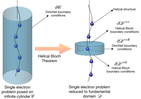
Figure 2: Illustration of the Helical Bloch Theorem (Theorem 2.3) for the case when the single electron Hamiltonian obeys the symmetries of the helical group ${\cal G}_{1}$.

2.2.2 Formulation of governing equations

In what follows, we will consider the helical structure to be at finite electronic temperature $T_{\text{e}}$ Kelvin and we will ignore spin polarization effects. For the sake of clarity of presentation, we will itemize the formulation/derivation of the various terms and equations, as we go along.

Electron Density and Density Matrix: A quantity of key importance in Kohn-Sham theory is the electron density. For a finite structure, such as a molecule or a cluster, this can be expressed in a straightforward manner in terms of the associated Kohn-Sham eigenstates and electronic occupations [33, 63]. For a helical structure however, care has to be taken to express this quantity due to the fact that there are effectively an infinite number of electrons associated with the structure. In what follows, motivated by rigorous mathematical results related to the description of electronic states in crystalline systems [101, 102, 103], we address this issue by defining the single particle density operator [104, 105, 106] in terms of the single electron Hamiltonian, and then expressing the electron density in terms of the diagonal of the density operator.

To clarify the above procedure, let us first consider a finite system (i.e., an isolated molecule or an atomic cluster, for example) in $\mathbb{R}^{3}$, and let the single electron Hamiltonian, the single particle density operator (or density matrix), and the electron density for the system be denoted as $H$, $\mathfrak{D}$ and $\varrho({\bf x})$ respectively. Then, $H$ and $\mathfrak{D}$ are related as [104, 105, 106]:

$$\mathfrak{D}=f_{T_{\text{e}}}(H)\,,$$ (56)

with $f_{T_{e}}(\cdot)$ denoting the Fermi-Dirac distribution function at electronic temperature $T_{\text{e}}$, i.e.:

$$f_{T_{e}}(y)=\frac{1}{1+\exp\big{(}{\frac{y\,-\,\lambda_{\text{F}}}{k_{\text{B}}T_{\text{e}}}}\big{)}}\,.$$ (57)

Here, $\lambda_{\text{F}}$ and $k_{\text{B}}$ denote the Fermi level and the Boltzmann constant respectively. Due to this definition, $\mathfrak{D}$ turns out to be a trace-class operator on $\textsf{L}^{2}(\mathbb{R}^{3})$, even though $H$ is (generically) an unbounded self-adjoint operator on the same space. Assuming $H$ has a pure point spectrum, denoting the eigenvalues of $H$ as $\omega_{j}\in\mathbb{R}$, and the corresponding eigenvectors as $\upsilon_{j}\in\textsf{L}^{2}(\mathbb{R}^{3})$, we may express $H$ using its spectral representation as:

$$H=\sum_{j=1}^{\infty}\omega_{j}\,\upsilon_{j}\otimes\overline{\upsilon_{j}}\,.$$ (58)

Using this form we see that the action of $H$ on any $f\in\text{Dom.}(H)$ is expressible as:

$$Hf=\sum_{j=1}^{\infty}\omega_{j}\,\langle f,\upsilon_{j}\rangle_{\textsf{L}^{2}(\mathbb{R}^{3})}\,\upsilon_{j}\,,$$ (59)

and that $\mathfrak{D}$ can be expressed by means of spectral mapping [95] as:

$$\mathfrak{D}=\sum_{j=1}^{\infty}f_{T_{e}}(\omega_{j})\,\upsilon_{j}\otimes\overline{\upsilon_{j}}$$ (60)

Due to this definition, the action of $\mathfrak{D}$ on any $f\in\textsf{L}^{2}(\mathbb{R}^{3})$ can be expressed as:

$$\mathfrak{D}f=\sum_{j=1}^{\infty}f_{T_{e}}(\omega_{j})\,\langle f,\upsilon_{j}\rangle_{\textsf{L}^{2}(\mathbb{R}^{3})}\,\upsilon_{j}\,,$$ (61)

and it makes sense to write $\mathfrak{D}$ in coordinate form as:

$$\mathfrak{D}({\bf x},{\bf y})=\sum_{j=1}^{\infty}f_{T_{e}}(\omega_{j})\,\upsilon_{j}({\bf x})\otimes\overline{\upsilon_{j}({\bf y})}\,,$$ (62)

for ${\bf x},{\bf y}\in\mathbb{R}^{3}$. In this setting, the electron density $\varrho({\bf x})$ can be identified in terms of the diagonal of $\mathfrak{D}$, i.e.,

$$\varrho({\bf x})=2\,\mathfrak{D}({\bf x},{\bf x})\,,$$ (63)

which leads to the well-known expression from Kohn-Sham theory [25] (also see footnote 33):

$$\varrho({\bf x})=2\,\sum_{j=1}^{\infty}f_{T_{e}}(\omega_{j})\,\lvert\upsilon_{j}({\bf x})\rvert^{2}\,.$$ (64)

Now, coming back to the case of the helical structure, we would analogously like to connect the single electron Hamiltonian $\mathfrak{H}$, the single particle density operator ${\Gamma}$ and the electron density $\rho({\bf x})$. Accordingly, we define:

$${\Gamma}=f_{T_{\text{e}}}(\mathfrak{H})\,,$$ (65)

as an operator on $\textsf{L}^{2}({\cal C})$. The issue however, is that $\mathfrak{H}$ does not admit a representation similar to eq. 58, and so the above definition does not immediately lead to transparent expressions for the electron density or the density operator in coordinate representation. To adress this, it is useful to first recast eq. 65 in terms of helical Bloch states. The apparatus of direct integrals [88, 107], discussed in B, allows us to do this in a mathematically rigorous manner. The key result from the appendix is that the helical Bloch-Floquet transform allows the single electron Hamiltonian to be “block-diagonalized” into a set of problems associated with the helical Bloch states that are posed over the fundamental domain, i.e.:

$${\cal U}\,\mathfrak{H}\,{\cal U}^{-1}=\int_{\mathfrak{I}}^{\oplus}\mathfrak{H}_{\eta}\,d\eta\,.$$ (66)

Here, as before, $\mathfrak{H}$ represents the operator $-\frac{1}{2}\Delta+V({\bf x})$ over the cylinder ${\cal C}$ along with the boundary condition $\psi({\bf x})=0$ for ${\bf x}\in\partial{\cal C}$. The potential $V({\bf x})$ is group invariant (eq. 15) and the unitary operator ${\cal U}:\textsf{L}^{2}({{\cal C}})\to\textsf{L}^{2}({{\cal D}}\times\mathfrak{I})$ represents the helical Bloch-Floquet transform (eq. 38). The operators $\{\mathfrak{H}_{\eta}\}_{\eta\in\mathfrak{I}}$ represent the fibers of $\mathfrak{H}$ (in the sense of direct integrals) and are closely related to the operators $\mathfrak{h}_{\eta}^{\textsf{aux}}$ introduced in the proof of Theorem 2.3 (eq. 25). Specifically, for each $\eta\in\mathfrak{I}$, the operator $\mathfrak{H}_{\eta}$ represents the operator $-\frac{1}{2}\Delta+V({\bf x})$ over the interior of the fundamental domain (i.e., the set ${\cal D}$) along with the boundary conditions $\psi(\Upsilon_{\mathsf{h}}\circ{\bf x})=e^{-i2\pi\eta}\,\psi({\bf x})$, ${\bf R}_{2\pi\alpha}^{-1}\nabla\psi(\Upsilon_{\mathsf{h}}\circ{\bf x})=e^{-i2\pi\eta}\,\nabla\psi({\bf x})$ for ${\bf x}\in\partial{\cal D}^{\,z=0}$ and, $\psi({\bf x})=0$ for ${\bf x}\in\partial{\cal D}^{\,r=R}$. The eigenstates of the operators $\{\mathfrak{H}_{\eta}\}_{\eta\in\mathfrak{I}}$ are precisely the helical bands $\Lambda=\{\lambda_{j}(\eta):\eta\in\mathfrak{I},j\in\mathbb{N}\}$ and the helical Bloch states $\Psi=\{\psi_{j}(\cdot;\eta):\eta\in\mathfrak{I},j\in\mathbb{N}\}$ restricted to the region ${\cal D}$.

Above, eq. 66 expresses that $\mathfrak{H}$ is unitarily equivalent to a “block-diagonal” operator whose “blocks” $\mathfrak{H}_{\eta}$ are indexed by $\eta\in\mathfrak{I}$. Therefore, upon computing $\Gamma$ using eq. 65, we can expect to obtain another operator which is unitarily equivalent to a block-diagonal operator with blocks $\big{\{}\Gamma_{\eta}=f_{T_{\text{e}}}(\mathfrak{H}_{\eta})\big{\}}_{\eta\in\mathfrak{I}}$. Since the function $f_{T_{e}}(\cdot)$ is analytic [108], these statements can be made mathematically precise by making use of the properties of the direct integral representation [88, Theorem XIII.85]. Thus, we may write for the density matrix $\Gamma$ (as an operator on $\textsf{L}^{2}({{\cal C}})$):

$${\cal U}\,\Gamma\,{\cal U}^{-1}=\int_{\mathfrak{I}}^{\oplus}\Gamma_{\eta}\,d\eta\,=\int_{\mathfrak{I}}^{\oplus}f_{T_{\text{e}}}(\mathfrak{H}_{\eta})\,d\eta\,.$$ (67)

Next, if we are able to express $f_{T_{\text{e}}}(\mathfrak{H}_{\eta})$ in a transparent form, we may be able to further simplify the expression for $\Gamma$. Accordingly, we write the operators $\mathfrak{H}_{\eta}$ using spectral representation [109, 110, 95] as:

$$\mathfrak{H}_{\eta}=\sum_{j=1}^{\infty}\lambda_{j}(\eta)\,\psi_{j}(\cdot;\eta)\otimes\overline{\psi_{j}(\cdot;\eta)}\,,$$ (68)

and obtain:

$$\Gamma_{\eta}=f_{T_{\text{e}}}(\mathfrak{H}_{\eta})=\sum_{j=1}^{\infty}f_{T_{\text{e}}}\big{(}\lambda_{j}(\eta)\big{)}\,\psi_{j}(\cdot;\eta)\otimes\overline{\psi_{j}(\cdot;\eta)}\,.$$ (69)

Thus, as an operator on $\textsf{L}^{2}({{\cal C}})$, the density matrix admits the representation:

$${\Gamma}={\cal U}^{-1}\,\bigg{(}\int_{\mathfrak{I}}^{\oplus}\!f_{T_{\text{e}}}(\mathfrak{H}_{\eta})\,d\eta\bigg{)}\,{\cal U}={\cal U}^{-1}\,\bigg{(}\int_{\mathfrak{I}}^{\oplus}\!\sum_{j=1}^{\infty}f_{T_{\text{e}}}\big{(}\lambda_{j}(\eta)\big{)}\,\psi_{j}(\cdot;\eta)\otimes\overline{\psi_{j}(\cdot;\eta)}\,d\eta\bigg{)}\,{\cal U}\,.$$ (70)

While describing quantities over the fundamental domain, it is more appropriate and easier to deal with the density matrix as expressed as an operator on $\textsf{L}^{2}({{\cal D}}\times\mathfrak{I})$. This can be written as $\tilde{\Gamma}={\cal U}\,\Gamma\,{\cal U}^{-1}$ (i.e., the right hand side of eq. 67), and it admits the following expression in coordinate representation (with ${\bf x},{\bf y}\in{\cal D}$):

$$\tilde{\Gamma}({\bf x},{\bf y})=\int_{\mathfrak{I}}^{\oplus}\!\sum_{j=1}^{\infty}\,f_{T_{\text{e}}}\big{(}\lambda_{j}(\eta)\big{)}\,\psi_{j}({\bf x};\eta)\otimes\overline{\psi_{j}({\bf y};\eta)}\,d\eta\,.$$ (71)

Now writing:

$$\rho({\bf x})=2\,\tilde{\Gamma}({\bf x},{\bf x})\,,$$ (72)

we see that the electron density can be expressed as (for ${\bf x}\in{\cal D}$):

$$\rho({\bf x})=2\int_{\mathfrak{I}}\sum_{j=1}^{\infty}\,f_{T_{e}}\big{(}\lambda_{j}(\eta)\big{)}\,\lvert\psi_{j}({\bf x};\eta)\rvert^{2}\,d\eta\,.$$ (73)

It is easy to see from the above expression that the electron density is group invariant and also obeys a zero-Dirichlet boundary condition on the lateral surface of ${\cal D}$ (i.e., for ${\bf x}\in\partial{\cal D}^{\,r=R}$). It is also apparent from the expression for the density matrix (eq. 71) that the following invariance relationship holds for any $m\in\mathbb{Z}$ and ${\bf x},{\bf y}\in{\cal D}$:

$$\tilde{\Gamma}({\bf x},{\bf y})=\tilde{\Gamma}(\Upsilon^{m}_{\mathsf{h}}\circ{\bf x},\Upsilon^{m}_{\mathsf{h}}\circ{\bf y})\,.$$ (75)

For notational simplicity, it is convenient to introduce the scalars $g_{j}(\eta)=f_{T_{e}}\big{(}\lambda_{j}(\eta)\big{)}$, i.e. the thermalized occupation numbers of the electronic states of the system, that appear in eqs. 73, 71 and 70. We will denote the collection of occupation numbers as $\mathfrak{G}=\big{\{}g_{j}(\eta)=f_{T_{e}}\big{(}\lambda_{j}(\eta)\big{)}:\eta\in\mathfrak{I},j\in\mathbb{N}\}$.

The electron density for an extended system is expected to obey the constraint of having a fixed number of electrons per unit fundamental domain of the system, even though the electronic states themselves are delocalized over the entire structure [44, 26]. Denoting the number of electrons per unit cell as $N_{\text{e}}$, in our case, this leads to:

$$\int_{{\cal D}}\rho({\bf x})\,d{\bf x}=N_{\text{e}}\,,$$ (76)

from which, using the orthonormality of the Bloch states over ${\cal D}$, follows the constraint:

$$2\int_{\mathfrak{I}}\sum_{j=1}^{\infty}\,f_{T_{e}}\big{(}\lambda_{j}(\eta)\big{)}\,d\eta=2\int_{\mathfrak{I}}\sum_{j=1}^{\infty}g_{j}(\eta)=N_{\text{e}}\,.$$ (77)

In practice, the above equation can be used to compute the Fermi-level ($\lambda_{\text{F}}$) of the system. It also follows from this discussion that the density matrix $\Gamma$ on $\textsf{L}^{2}({\cal C})$ is locally trace class.

Electronic Free Energy (per unit fundamental domain): With the above expressions in place, we can now use an energy-minimization formalism to deduce the governing equations of Kohn-Sham theory for the helical structure. Since the structure is infinite, the quantity of primary importance in this regard is the electronic free energy per unit fundamental domain, denoted here as ${\cal F}(\Lambda,\Psi,{\cal P}_{{\cal G}_{1}},{\cal D},{\cal G}_{1})$. This notation emphasizes the dependence of this quantity on the helical Bloch states, the helical Bloch bands, the positions of the simulated atoms ${\cal P}_{{\cal G}_{1}}=\big{\{}{\bf x}_{k}\big{\}}_{k=1}^{M_{{\cal G}_{1}}}$ within the fundamental domain, (the interior of) the fundamental domain and the helical group itself. Following [63], we express this quantity within the pseudopotential [113, 114] and Local Density Approximations [25] as:

$${\cal F}(\Lambda,\Psi,{\cal P}_{{\cal G}_{1}},{\cal D},{\cal G}_{1})=T_{\text{s}} (\Lambda,\Psi,{\cal D},{\cal G}_{1})\,+\,E_{\text{xc}}(\rho,{\cal D})\,+\,K(\Lambda,\Psi,{\cal P}_{{\cal G}_{1}},{\cal D},{\cal G}_{1})$$

$$+E_{\text{el}}(\rho,{\cal P}_{{\cal G}_{1}},{\cal D},{\cal G}_{1})\,-\,T_{\text{e}}\,S(\Lambda)\,,$$ (78)

with the terms on the right-hand side representing the kinetic energy of the electrons, the exchange correlation energy, the nonlocal pseudopotential energy, the electrostatic energy and the electronic entropy contribution, respectively. We now discuss each of the terms in the above equation in detail.

Kinetic Energy Term: The first term on the right-hand side of the above expression represents the kinetic energy of the electrons per unit fundamental domain. To motivate this term, we recall that for a finite system (in ${\mathbb{R}^{3}}$) with single particle density matrix $\mathfrak{D}$, the kinetic energy can be expressed as [101, 106, 105]:

$$T_{\text{s}}^{\text{finite}}=2\,\text{Tr.}\big{[}-\frac{1}{2}\Delta\,\mathfrak{D}\big{]}\,,$$ (79)

with $\text{Tr.}[\cdot]$ denoting the operator trace (of a trace-class operator on $\textsf{L}^{2}(\mathbb{R}^{3})$). Analogously, it would make sense to consider the trace per unit fundamental domain in case of the helical structure. As described in B, for an operator ${\cal A}$ which is invariant under the group ${\cal G}_{1}$ and which is locally trace-class, it is possible to assign meaning to the trace per unit fundamental domain by means of the direct integral decomposition. Specifically, if the helical Bloch-Floquet transform block-diagonalizes the operator into its fibers as:

$${\cal U}\,{\cal A}\,{\cal U}^{-1}=\int_{\mathfrak{I}}^{\oplus}{\cal A}_{\eta}\,d\eta\,,$$ (80)

then the trace per unit cell (denoted $\underline{\text{Tr.}}[\cdot]$ henceforth) can be expressed as:

$$\underline{\text{Tr.}}[{\cal A}]=\int_{\mathfrak{I}}\!\text{Tr.}[{\cal A}_{\eta}]\,d\eta\,,$$ (81)

with the trace inside the integral signifying the usual operator trace in $\textsf{L}^{2}({\cal D})$. The expression for the kinetic energy per unit fundamental domain for the helical structure therefore boils down to:

$$T_{\text{s}} (\Lambda,\Psi,{\cal D},{\cal G}_{1})=2\,\underline{\text{Tr.}}\big{[}-\frac{1}{2}\Delta\,{\Gamma}\big{]}=2\int_{\mathfrak{I}}\!\text{Tr.}\bigg{[}\big{(}-\frac{1}{2}\Delta\,{\Gamma}\big{)}_{\eta}\bigg{]}\,d\eta\,.$$ (83)

We now write $\big{(}-\frac{1}{2}\Delta{\Gamma}\big{)}_{\eta}$ as $(-\frac{1}{2}\Delta)_{\eta}{\Gamma}_{\eta}$, observe that ${\Gamma}_{\eta}$ is already available from eq. 69. Next, based on the discussion in B, we note that the fibers of the Laplacian on $\textsf{L}^{2}({\cal C})$ are simply the Laplacian operators on $\textsf{L}^{2}({\cal D})$ with ($\eta$ -dependent) helical Bloch boundary conditions. Since the states $\psi_{j}({\bf x};\eta)$ already satisfy these boundary conditions, and they form a basis of $\textsf{L}^{2}({\cal D})$, it follows that:

$$T_{\text{s}}(\Lambda,\Psi,{\cal D},{\cal G}_{1}) =2\int_{\mathfrak{I}}\bigg{[}\sum_{j=1}^{\infty}f_{T_{\text{e}}}\big{(}\lambda_{j}(\eta)\big{)}\int_{{\cal D}}-\frac{1}{2}\Delta\psi_{j}({\bf x};\eta)\,\overline{\psi_{j}({{\bf x}};\eta)}\,d{\bf x}\bigg{]}d\eta$$

$$=\int_{\mathfrak{I}}\sum_{j=1}^{\infty}f_{T_{\text{e}}}\big{(}\lambda_{j}(\eta)\big{)}\big{\langle}{\Delta\psi_{j}(\cdot;\eta)},{\psi_{j}(\cdot;\eta)}\big{\rangle}_{\textsf{L}^{2}({\cal D})}\,d\eta$$

$$=\int_{\mathfrak{I}}\sum_{j=1}^{\infty}g_{j}(\eta)\big{\langle}{\Delta\psi_{j}(\cdot;\eta)},{\psi_{j}(\cdot;\eta)}\big{\rangle}_{\textsf{L}^{2}({\cal D})}\,d\eta\,.$$ (84)

Exchange-Correlation Term: The second term on the right-hand side of eq. 78 represents the exchange correlation energy of the electrons per unit fundamental domain. Within the Local Density Approximation (LDA) [25], it can be written as:

$$E_{\text{xc}}(\rho,{\cal D})=\int_{{\cal D}}\varepsilon_{\text{xc}}[\rho({\bf x})]\,\rho({\bf x})\,d{\bf x}\,.$$ (85)

Note that it is also possible to modify this expression to use more sophisticated exchange correlation functionals such as the Generalized Gradient Approximation [115] and this will have little bearing on our subsequent discussion.

Nonlocal Pseudopotential Energy Term: The third term on the right-hand side of eq. 78 represents the energetic contribution from the nonlocal part of the pseudopotential and models the effect of electronic core states. For a finite system of $N_{\text{at}}$ atoms located at the points $\{{\bf p}_{k}\in\mathbb{R}^{3}\}_{k=1}^{N_{\text{at}}}$, if the single particle electron density is denoted as $\mathfrak{D}$, then this term has the following form:

$$K^{\text{finite}}=2\,\text{Tr.}\big{[}{\cal V}^{\text{nl}}\,\mathfrak{D}\big{]}\,.$$ (86)

The operator ${\cal V}^{\text{nl}}$ in the above equation is expressible in Kleinman-Bylander form [116] as :

$${\cal V}^{\text{nl}}=\sum_{k=1}^{N_{\text{at}}}\sum_{p\in{\cal N}_{k}}\gamma_{k,p}\,\chi_{k,p}(\cdot;{\bf p}_{k})\,{\otimes}\,\overline{\chi_{k,p}(\cdot;{\bf p}_{k})}\,.$$ (87)

Here, ${\cal N}_{k}$ denotes the collection of projectors associated with the atom at ${\bf p}_{k}$, $\chi_{k,p}$ are the projection functions, and $\gamma_{k,p}$ are the corresponding normalization constants. The functions $\chi_{k,p}$ are themselves expressible in terms of atomic orbitals and are usually supported in a small region of space by design [117]. To obtain the correct analog of this expression for the helical structure i.e., the nonlocal pseudopotential energy per unit fundamental domain, it is useful to recall that this contribution to the energy is tied to the atoms in the fundamental domain as well as the electronic states in the system. It is of a somewhat different nature as compared to the kinetic energy term for instance, in which case the electrons are the only contributing source. Since the electrons in the extended structure are delocalized, the trace per unit fundamental domain leads to the appropriate expression in that case. In case of the nonlocal pseudopotential energy term however, the contribution from the electrons is delocalized, while those from the atoms are not. With this in mind, we now focus on the atoms in the fundamental domain, and denote the non-local pseudoptential operator associated with these atoms as:

$${\cal V}^{\text{nl}}_{{\cal D}}=\sum_{k=1}^{M_{{\cal G}_{1}}}\sum_{p\in{\cal N}_{k}}\gamma_{k,p}\,\chi_{k,p}(\cdot;{\bf x}_{k})\,{\otimes}\,\overline{\chi_{k,p}(\cdot;{\bf x}_{k})}\,.$$ (88)

Then, in analogy with eq. 86, the nonlocal pseudopotential energy per unit fundamental domain in case of the helical structure can be written by considering the action of ${\cal V}^{\text{nl}}_{{\cal D}}$ to the density matrix operator defined in eq. 70, i.e.:

$$K=2\,\text{Tr.}[\,{\cal V}^{\text{nl}}_{{\cal D}}\,{\Gamma}\,]\,.$$ (89)

To simplify this expression, we employ eqs. 67, 70, the unitarity of the operator ${\cal U}$, as well as the invariance of the trace under unitary transformations to obtain:

$$K=2\,\text{Tr.}[\,{\cal V}^{\text{nl}}_{{\cal D}}\,{\cal U}^{-1}\,\tilde{\Gamma}\,{\cal U}\,]=2\,\text{Tr.}[\,{\cal U}^{-1}\,{\cal U}\,{\cal V}^{\text{nl}}_{{\cal D}}\,{\cal U}^{-1}\,\tilde{\Gamma}\,{\cal U}\,]=2\,\text{Tr.}[\,{\cal U}\,{\cal V}^{\text{nl}}_{{\cal D}}\,{\cal U}^{-1}\,\tilde{\Gamma}\,]\,.$$ (90)

Next, we observe that the operator $\widehat{{\cal V}}^{\text{nl}}_{{{\cal D}}}={\cal U}\,{\cal V}^{\text{nl}}_{{\cal D}}\,{\cal U}^{-1}$ acts on $\textsf{L}^{2}({\cal D}\times\mathfrak{I})$, and it admits a direct integral representation (i.e., $\widehat{{\cal V}}^{\text{nl}}_{{{\cal D}}}=\displaystyle\int_{\mathfrak{I}}^{\oplus}(\widehat{{\cal V}}^{\text{nl}}_{{{\cal D}}})_{\eta}\,d\eta$ ). The fibers of $\widehat{{\cal V}}^{\text{nl}}_{{{\cal D}}}$ can be written as :

$$(\widehat{{\cal V}}^{\text{nl}}_{{{\cal D}}})_{\eta}=({\cal U}\,{\cal V}^{\text{nl}}_{{\cal D}}\,{\cal U}^{-1})_{\eta} ={\cal U}\,\bigg{(}\sum_{k=1}^{M_{{\cal G}_{1}}}\sum_{p\in{\cal N}_{k}}\gamma_{k,p}\,\chi_{k,p}(\cdot;{\bf x}_{k})\,{\otimes}\,\overline{\chi_{k,p}(\cdot;{\bf x}_{k})}\bigg{)}\,{\cal U}^{-1}$$

$$=\sum_{k=1}^{M_{{\cal G}_{1}}}\sum_{p\in{\cal N}_{k}}\gamma_{k,p}\,\,{\cal U}\chi_{k,p}(\cdot;\eta;{\bf x}_{k})\,{\otimes}\,\overline{{\cal U}\chi_{k,p}(\cdot;\eta;{\bf x}_{k})}\,.$$ (91)

In what follows, for the sake of brevity, we will denote the helical Bloch-Floquet transform of the projection functions, i.e., ${\cal U}\chi_{k,p}(\cdot;\eta;{\bf x}_{k})$ as $\hat{\chi}_{k,p}(\cdot;\eta;{\bf x}_{k})$ and note that they can be represented via eq. 38 (for ${\bf x}\in{\cal D}$ and $\eta\in\mathfrak{I}$ as):

$$\hat{\chi}_{k,p}({\bf x};\eta;{\bf x}_{k})={\cal U}\chi_{k,p}({\bf x};\eta;{\bf x}_{k})=\sum_{m\in\mathbb{Z}}{\chi}_{k;p}(\Upsilon^{m}_{\mathsf{h}}\circ{\bf x};{\bf x}_{k})\,e^{i2\pi m\eta}\,.$$ (93)

With this notation, using properties tensor products, as well as eqs. 93 and 71, we may rewrite eq. 90 as:

$$K(\Lambda,\Psi, {\cal P}_{{\cal G}_{1}},{\cal D},{\cal G}_{1})$$

$$=2\,\text{Tr.}[\,{\cal U}\,{\cal V}^{\text{nl}}_{{\cal D}}\,{\cal U}^{-1}\,\tilde{\Gamma}\,]=2\,\text{Tr.}[\,\widehat{{\cal V}}^{\text{nl}}_{{{\cal D}}}\,\tilde{\Gamma}\,]$$

$$=2\,\text{Tr.}\Bigg{[}\,\bigg{(}\int_{\mathfrak{I}}^{\oplus}(\widehat{{\cal V}}^{\text{nl}}_{{{\cal D}}})_{\eta}\,d\eta\bigg{)}\,\bigg{(}\int_{\mathfrak{I}}^{\oplus}\Gamma_{\eta}\,d\eta\bigg{)}\,\Bigg{]}$$

$$=2\,\text{Tr.}\Bigg{[}\bigg{(}\int_{\mathfrak{I}}^{\oplus}\sum_{k=1}^{M_{{\cal G}_{1}}}\sum_{p\in{\cal N}_{k}}\gamma_{k,p}\,\hat{\chi}_{k,p}(\cdot;\eta;{\bf x}_{k})\,{\otimes}\,\overline{\hat{\chi}_{k,p}(\cdot;\eta;{\bf x}_{k})}\,d\eta\bigg{)}$$

$$\quad\quad\quad\quad\bigg{(}\int_{\mathfrak{I}}^{\oplus}\!\sum_{j=1}^{\infty}\,f_{T_{\text{e}}}\big{(}\lambda_{j}(\eta)\big{)}\,\psi_{j}(\cdot;\eta)\,{\otimes}\,\overline{\psi_{j}(\cdot;\eta)}\,d\eta\,\bigg{)}\Bigg{]}\,.$$

$$=2\,\text{Tr.}\Bigg{[}\int_{\mathfrak{I}}^{\oplus}\bigg{(}\sum_{k=1}^{M_{{\cal G}_{1}}}\sum_{p\in{\cal N}_{k}}\gamma_{k,p}\sum_{j=1}^{\infty}f_{T_{\text{e}}}\big{(}\lambda_{j}(\eta)\big{)}\big{(}\hat{\chi}_{k,p}(\cdot;\eta;{\bf x}_{k})\psi_{j}(\cdot;\eta)\big{)}$$

$$\quad\quad\quad\quad\quad\quad\quad\quad\quad\quad\quad\quad\quad\quad\quad\quad\quad\;\otimes\overline{\big{(}\hat{\chi}_{k,p}(\cdot;\eta;{\bf x}_{k})\,\psi_{j}(\cdot;\eta)\big{)}}\bigg{)}\,d\eta\,\Bigg{]}$$ (94)

Now using the definition of the trace and that the helical Bloch states are a basis, this reduces to:

$$K(\Lambda,\Psi,{\cal P}_{{\cal G}_{1}},{\cal D},{\cal G}_{1})$$

$$=2\,\sum_{k=1}^{M_{{\cal G}_{1}}}\sum_{p\in{\cal N}_{k}}\gamma_{k,p}\int_{\mathfrak{I}}\bigg{(}\sum_{j=1}^{\infty}\,f_{T_{\text{e}}}\big{(}\lambda_{j}(\eta)\big{)}\big{\langle}{\hat{\chi}_{k,p}(\cdot;\eta;{\bf x}_{k})},{\psi_{j}(\cdot;\eta)}\big{\rangle}_{\textsf{L}^{2}({\cal D})}$$

$$\quad\quad\quad\quad\quad\quad\quad\quad\quad\quad\quad\quad\times\overline{\big{\langle}{\hat{\chi}_{k,p}(\cdot;\eta;{\bf x}_{k})},{\psi_{j}(\cdot;\eta)}\big{\rangle}}_{\textsf{L}^{2}({\cal D})}\bigg{)}\,d\eta$$

$$=2\,\sum_{k=1}^{M_{{\cal G}_{1}}}\sum_{p\in{\cal N}_{k}}\sum_{j=1}^{\infty}\gamma_{k,p}\int_{\mathfrak{I}}\bigg{(}f_{T_{\text{e}}}\big{(}\lambda_{j}(\eta)\big{)}\bigg{\lvert}{\big{\langle}{\hat{\chi}_{k,p}(\cdot;\eta;{\bf x}_{k})},{\psi_{j}(\cdot;\eta)}\big{\rangle}}_{\textsf{L}^{2}({\cal D})}\bigg{\rvert}^{2}\bigg{)}\,d\eta$$

$$=2\,\sum_{k=1}^{M_{{\cal G}_{1}}}\sum_{p\in{\cal N}_{k}}\sum_{j=1}^{\infty}\gamma_{k,p}\int_{\mathfrak{I}}\bigg{(}g_{j}(\eta)\bigg{\lvert}{\big{\langle}{\hat{\chi}_{k,p}(\cdot;\eta;{\bf x}_{k})},{\psi_{j}(\cdot;\eta)}\big{\rangle}}_{\textsf{L}^{2}({\cal D})}\bigg{\rvert}^{2}\bigg{)}\,d\eta$$ (96)

Electrostatic Energy Term: We now discuss the contribution of the electrostatic interaction energy to the free energy per unit fundamental domain. This is the fourth term on the right-hand side of eq. 78. Often, it is computationally advantageous to express this term using a so-called local formulation [118, 119, 120, 63], as we now do. For a finite system with atomic nuclei located at the points $\{{\bf p}_{k}\in\mathbb{R}^{3}\}_{k=1}^{N_{\text{at}}}$ and electron density $\rho$, this term takes the form of the following optimization problem in the total electrostatic potential:

$${E}_{\text{el}}^{\text{finite}}=\max_{\Phi}\bigg{\{}-\frac{1}{8\pi}\int_{\mathbb{R}^{3}}\lvert\nabla\Phi\rvert^{2}\,d{\bf x}+\int_{\mathbb{R}^{3}}(\rho+b^{\text{finite}})\Phi\,d{\bf x}\bigg{\}}+E_{\text{sc}}^{\text{finite}}({\bf p}_{1},{\bf p}_{2},\ldots,{\bf p}_{k})\,.$$ (97)

Here $b^{\text{finite}}$ represents the total nuclear pseudocharge for the finite set of nuclei, and can be expressed in terms of the individual nuclear pseudocharges $\big{\{}b_{k}({\bf x};{\bf p}_{k})\big{\}}_{k=1}^{{N_{\text{at}}}}$ as:

$$b^{\text{finite}}({\bf x})=\sum_{k=1}^{N_{\text{at}}}b_{k}({\bf x};{\bf p}_{k})\,,$$ (98)

and the term $E_{\text{sc}}^{\text{finite}}({\bf p}_{1},{\bf p}_{2},\ldots,{\bf p}_{k})$ corrects for self-interactions and overlaps of the nuclear pseudocharges [119]. Note that by design, the individual nuclear pseudocharges are usually smooth, radially symmetric functions centered at the nuclear positions, they have compact support, and they integrate to the (valence) nuclear charge of the nucleus in question. The electrostatic potential $\Phi$ that solves the maximization problem in eq. 97 is the Newtonian potential associated with the net charge in the system:

$$\Phi({\bf x})=\int_{\mathbb{R}^{3}}\frac{\rho({\bf y})+b^{\text{finite}}({\bf y})}{\lVert{\bf x}-{\bf y}\rVert_{\mathbb{R}^{3}}}\,d{\bf y}$$ (99)

To extend the above formulation to a helical structure, we first write the total nuclear pseudocharge at any point ${\bf x}\in{\cal C}$ in terms of the pseudocharges of the atoms in the fundamental domain as:

$$b({\bf x},{\cal P}_{{\cal G}_{1}},{\cal G}_{1})=\sum_{m\in\mathbb{Z}}\sum_{k=1}^{M_{{\cal G}_{1}}}b_{k}({\bf x};\Upsilon^{m}_{\mathsf{h}}\circ{\bf x}_{k})\,,$$ (100)

and observe that this quantity is group invariant owing to the aforementioned properties of the individual nuclear pseudocharges [40]. Since the electron density is group invariant as well, it follows that the net electrostatic potential $\Phi$ expressed as:

$$\Phi({\bf x})=\int_{{\cal C}}\frac{\rho({\bf y})+b({\bf y},{\cal P}_{{\cal G}_{1}},{\cal G}_{1})}{\lVert{\bf x}-{\bf y}\rVert_{\mathbb{R}^{3}}}\,d{\bf y}\,,$$ (101)

is also group invariant [8]. Therefore, we may use $\Phi,b$ and $\rho$ as defined over the fundamental domain, to define the analog of eq. 97 for the helical structure as:

$$E_{\text{el}}(\rho,{\cal P}_{{\cal G}_{1}},{\cal D},{\cal G}_{1})=\max_{\Phi}\bigg{\{}- \frac{1}{8\pi}\int_{{\cal D}}\lvert\nabla\Phi\rvert^{2}\,d{\bf x}+\int_{{\cal D}}\bigg{(}\rho({\bf x})+b({\bf x},,{\cal P}_{{\cal G}_{1}},{\cal G}_{1})\bigg{)}\Phi({\bf x})\,d{\bf x}\bigg{\}}$$

$$+E_{\text{sc}}({\cal P}_{{\cal G}_{1}},{\cal G}_{1},{\cal D})\,.$$ (102)

For the sake of brevity, we omit the details of the form of the corrections due to self interactions and overlaps of the nuclear pseudocharges, as reduced to the fundamental domain (i.e., the term $E_{\text{sc}}({\cal P}_{{\cal G}_{1}},{\cal G}_{1},{\cal D})$ above) and instead point to [40, 119] for relevant information.

Electronic Entropy Term: Finally, the last term on the right-hand side of 78 represents the electronic entropy contribution to the free energy. Following [121], this term can be expressed for a finite system with density matrix $\mathfrak{D}$ as:

$$S^{\text{finite}}=-2\,k_{\text{B}}\text{Tr.}[\,\mathfrak{D}\,\log(\mathfrak{D})+({\cal I}-\mathfrak{D})\,\log({\cal I}-\mathfrak{D})]\,,$$ (103)

with ${\cal I}$ denoting the identity operator. To obtain the analogous expression for the case of the helical structure, we work with the trace per unit fundamental domain instead. This gives us:

$$S =-2\,k_{\text{B}}\,\underline{\text{Tr.}}\bigg{[}\,{\Gamma}\,\log({\Gamma})+({\cal I}-{\Gamma})\,\log({\cal I}-{\Gamma})\,\bigg{]}$$

$$=-2\,k_{\text{B}}\int_{\mathfrak{I}}\text{Tr.}[{\Gamma}_{\eta}\,\log({\Gamma}_{\eta})+({\cal I}-{\Gamma}_{\eta})\,\log({\cal I}-{\Gamma}_{\eta})]\,d\eta\,.$$ (104)

By means of spectral mapping [95], the use of eq. 69, and by noting again that the helical Bloch states $\psi_{j}({\bf x};\eta)$ are a basis of $\textsf{L}^{2}({\cal D})$, we readily obtain:

$$S(\Lambda)=$$

$$-2\,k_{\text{B}}\int_{\mathfrak{I}}\bigg{[}\sum_{j=1}^{\infty}f_{T_{\text{e}}}\big{(}\lambda_{j}(\eta)\big{)}\,\log\big{(}f_{T_{\text{e}}}\big{(}\lambda_{j}(\eta)\big{)}\big{)}+\big{(}1-f_{T_{\text{e}}}\big{(}\lambda_{j}(\eta)\big{)}\big{)}\,\log\big{(}1-f_{T_{\text{e}}}\big{(}\lambda_{j}(\eta)\big{)}\big{)}\bigg{]}\,d\eta$$

$$=-2\,k_{\text{B}}\int_{\mathfrak{I}}\bigg{[}\sum_{j=1}^{\infty}g_{j}(\eta)\,\log\big{(}g_{j}(\eta)\big{)}+\big{(}1-g_{j}(\eta)\big{)}\,\log\big{(}1-g_{j}(\eta)\big{)}\bigg{]}\,d\eta$$ (105)

With the above terms explicitly defined, we now turn to the variational problem for deducing the governing equations.

Variational Problem and Kohn-Sham Equations: The variational problem for Kohn-Sham ground state of a given helical structure (i.e., the atomic coordinates in the fundamental domain, the fundamental domain and the helical group are held fixed) consists of minimizing the electronic free energy ${\cal F}(\Lambda,\Psi,{\cal P}_{{\cal G}_{1}},{\cal D},{\cal G}_{1})$ with respect to the helical Bloch states and the helical bands, subject to the constraint in eq. 77. In the literature, this minimization is often stated in terms of the helical Bloch states and the electronic occupation numbers instead [63, 34]. Along those lines, we may define $\widetilde{{\cal F}}(\mathfrak{G},\Psi,{\cal P}_{{\cal G}_{1}},{\cal D},{\cal G}_{1})={\cal F}(\Lambda,\Psi,{\cal P}_{{\cal G}_{1}},{\cal D},{\cal G}_{1})$ to write the variational problem as:

$$\widetilde{{\cal F}}_{0}({\cal P}_{{\cal G}_{1}},{\cal D},{\cal G}_{1})=\text{inf.}_{{\Psi,\mathfrak{G}}}\,\widetilde{{\cal F}}(\mathfrak{G},\Psi,{\cal P}_{{\cal G}_{1}},{\cal D},{\cal G}_{1})$$ (106)

subject to:

$$2\int_{\mathfrak{I}}\sum_{j=1}^{\infty}g_{j}(\eta)=N_{\text{e}}\,,$$ (107)

and the requirement that the states in $\Psi$ be helical Bloch states. This requires that for any $\psi_{j}(\cdot;\eta)\in\Psi$ and $m\in\mathbb{Z}$, we have $\psi_{j}(\Upsilon^{m}_{\mathsf{h}}\circ{\bf x};\eta)=e^{-i2\pi m\eta}\psi_{j}({\bf x};\eta)\,$, as well as the orthonormality condition between two helical Bloch states $\psi_{i}(\cdot;\eta),\psi_{j}(\cdot;\eta)\in\Psi$:

$$\langle\psi_{i}(\cdot;\eta),\psi_{j}(\cdot;\eta)\rangle_{\textsf{L}^{2}({\cal D})}=\delta_{i,j}\,.$$ (108)

We take variations of the above constrained minimization problem, and obtain the Euler-Lagrange equations as the following helical symmetry adapted Kohn-Sham equations over the fundamental domain:

$$\mathfrak{H}^{\text{KS}}_{[\mathfrak{G},\Psi,{\cal P}_{{\cal G}_{1}},{\cal D},{\cal G}_{1}]}\,\psi_{j}(\cdot;\eta)=\lambda_{j}(\eta)\,\psi_{j}(\cdot;\eta)\,\,\text{for}\,j\in\mathbb{N},\eta\in\mathfrak{I}\,.$$ (109)

Here, the helical symmetry adapted Kohn-Sham Hamiltonian operator (with its dependence on the helical Bloch sates, the occupation numbers, etc., made explicit) is:

$$\mathfrak{H}^{\text{KS}}_{[\mathfrak{G},\Psi,{\cal P}_{{\cal G}_{1}},{\cal D},{\cal G}_{1}]}\equiv-\frac{1}{2}\Delta+V_{\text{xc}}+\Phi+\widetilde{{\cal V}}^{\text{nl}}_{{\cal D}}\,,$$ (110)

in which $\displaystyle V_{\text{xc}}=\frac{\delta E_{\text{xc}}(\rho,{\cal D})}{\delta\rho}$ is the exchange correlation potential, $\Phi$ is the net electrostatic potential and satisfies the following symmetry adapted Poisson problem over the fundamental domain:

$$-\Delta\Phi =4\pi\,\big{(}\rho+b(\cdot,{\cal P}_{{\cal G}_{1}},{\cal G}_{1})\big{)}\,,$$

$$\Phi(\Upsilon_{\mathsf{h}}\circ{\bf x}) =\Phi({\bf x})\,,$$ (111)

and the operator $\widetilde{{\cal V}}^{\text{nl}}_{{\cal D}}={\cal U}\,{{\cal V}}^{\text{nl}}_{{\cal D}}\,{\cal U}^{-1}$ is as defined in eqs. 91 and 93.

Harris-Foulkes Functional: The above set of expressions represent a set of coupled nonlinear partial differential equations in the fields $\psi_{j}(\cdot;\eta)$ and the scalars $g_{j}(\eta)$. Once they have been solved self-consistently, the ground state electronic free energy $\widetilde{{\cal F}}_{0}({\cal P}_{{\cal G}_{1}},{\cal D},{\cal G}_{1})$ per unit fundamental domain can be computed through eq. 78. In practical calculations, since self-consistency is never achieved perfectly, a better estimate of the ground state electronic free energy may be found using the so-called Harris-Foulkes functional [122, 123]. This can be written in helical symmetry-adapted form, using quantities expressed over the fundamental domain as:

$${{\cal F}}^{\text{HF}}(\Lambda,\Psi, {\cal P}_{{\cal G}_{1}},{\cal D},{\cal G}_{1})=E_{\text{band}}(\Lambda)+E_{\text{xc}}(\rho,{\cal D})-\int_{{\cal D}}V_{\text{xc}}(\rho({\bf x}))\rho({\bf x})\,d{\bf x}$$

$$+\frac{1}{2}\int_{{\cal D}}\bigg{(}b({\bf x},,{\cal P}_{{\cal G}_{1}},{\cal G}_{1})-\rho({\bf x})\bigg{)}\Phi({\bf x})\,d{\bf x}+E_{\text{sc}}({\cal P}_{{\cal G}_{1}},{\cal G}_{1},{\cal D})-T_{\text{e}}\,S(\Lambda)\,.$$ (112)

All the quantities on the right-hand side of the above equation are easily interpreted based on earlier discussion, except the first one, i.e., $E_{\text{band}}(\Lambda)$, which represents the electronic band energy per unit fundamental domain. For a finite system with a single electron Hamiltonian $H$ and single particle density matrix $\mathfrak{D}$, this quantity is expressed as [106]:

$$E_{\text{band}}^{\text{finite}}=2\,\text{Tr.}[H\mathfrak{D}]\,.$$ (113)

Analogously, for the helical structure, we use the trace per unit fundamental domain to write:

$$E_{\text{band}}=2\underline{\text{Tr.}}[\,\mathfrak{H}{\Gamma}\,]=2\int_{\mathfrak{I}}\text{Tr.}[\,\mathfrak{H}_{\eta}{\Gamma}_{\eta}\,]\,d\eta\,.$$ (114)

Using eqs. 68 and 69 and using the completeness of the helical Bloch waves, we see that this is be expressible as:

$$E_{\text{band}}(\Lambda)=2\int_{\mathfrak{I}}\sum_{j=1}^{\infty}\lambda_{j}(\eta)f_{T_{\text{e}}}\big{(}\lambda_{j}(\eta)\big{)}\,d\eta=2\int_{\mathfrak{I}}\sum_{j=1}^{\infty}\lambda_{j}(\eta)\,g_{j}(\eta)\,d\eta$$ (115)

Atomic Forces: The Hellmann-Feynman forces on the atoms in the fundamental domain are (in Cartesian coordinates):

$$\mathbf{f}_{k}=-\frac{\partial\widetilde{{\cal F}}_{0}({\cal P}_{{\cal G}_{1}},{\cal D},{\cal G}_{1})}{\partial{\bf x}_{k}}\,.$$ (116)

By directly differentiating the various terms involved (eqs. 94, 102) we arrive at the following expression for $\mathbf{f}_{k}$ using quantities specified over the fundamental domain:

$$\mathbf{f}_{k} =\sum_{m\in\mathbb{Z}}({\bf R}_{2\pi m\alpha})^{-1}\int_{{\cal D}}\nabla b_{k}({\bf x};\Upsilon^{m}_{\mathsf{h}}\circ{\bf x}_{k})\Phi({\bf x})\,d{\bf x}-\frac{\partial E_{\text{sc}}({\cal P}_{{\cal G}_{1}},{\cal G}_{1},{\cal D})}{\partial{\bf x}_{k}}$$

$$-4\sum_{j=1}^{\infty}\Bigg{(}\int_{\mathfrak{I}}g_{j}(\eta)\sum_{p\in\mathcal{N}_{k}}\gamma_{k;p}\,\text{Re.}\Bigg{\{}\bigg{[}\int_{{\cal D}}\hat{\chi}_{k,p}({\bf x};\eta;{\bf x}_{k})\,\overline{\psi_{j}({\bf x};\eta)}\,d{\bf x}\bigg{]}$$

$$\quad\quad\quad\quad\quad\quad\quad\quad\quad\quad\quad\quad\quad\times\bigg{[}\int_{{\cal D}}\psi_{j}({\bf x};\eta)\,\overline{\frac{\partial\hat{\chi}_{k,p}({\bf x};\eta;{\bf x}_{k})}{\partial{\bf x}_{k}}}\,d{\bf x}\bigg{]}\Bigg{\}}\Bigg{)}\,d\eta$$ (118)

Here, Re. denotes the real part of the quantity in braces.

This completes a discussion of the derivation of the various physically relevant terms, as well as the form of the equations of Kohn-Sham theory, as applied to a helical structure associated with a helical group generated by a single element. Comments on modifications of the above equations while dealing with a structure associated with a helical group generated two elements, and a presentation of the final expressions/equations for that case in appear in C.

3 Numerical Implementation

The Kohn-Sham equations for a helical structure (i.e., eq. 109 or eq. 193) are a set of non-linear eigenvalue problems indexed by $\eta$ (as well as $\nu$ in case of the group ${\cal G}_{2}$) that are coupled to each other through the electron density $\rho$. The standard procedure for solving the equations of Kohn-Sham theory is through self-consistent field (SCF) iterations [25]. This amounts to starting from a reasonable guess of the electron density in the fundamental domain (e.g. superpositions of individual atomic densities, as is used in our simulations) and an appropriate set of trial orthonormal wavefunctions (randomly chosen in our simulations), and then evaluating the eigenstates of the Kohn-Sham operator with these guesses. Thus, a set of linear eigenvalue problems (i.e., those associated with the linearized Kohn-Sham operator evaluated at the given electron density) indexed by $\eta$ (as well as $\nu$ in case of the group ${\cal G}_{2}$) have to be solved. From this, the (trial) Fermi-level of the system and the (trial) occupation numbers maybe computed. The eigenfunctions and the occupation numbers may be then combined (in accordance with eq. 73 or eq. 181) to yield the trial electron density for the next step of the iterations. The above procedure has to be repeated till the difference in the electron density (or the effective potential) between successive iterations reaches below the desired convergence threshold. We will now discuss several features of this self-consistent solution process as implemented in the Helical DFT code.

3.1 Discretization of reciprocal space

Many quantities described in Section 2.2.2 and C involve integrals over $\eta\in\mathfrak{I}=[-\frac{1}{2},\frac{1}{2})$ (as well as normalized summations over $\nu\in\{0,{1},2,\ldots,{\mathfrak{N}-1}\}$ for the group ${\cal G}_{2}$). To evaluate such integrals numerically, we employ quadrature based on the Monkhorst-Pack scheme [125]. Specifically, we sample the interval $\mathfrak{I}$ using a grid of $N_{\eta}$ points, and write:

$$\int_{\mathfrak{I}}f(\eta)\,d\eta\approx\sum_{{b=1}}^{N_{\eta}}\,w_{b}\,f(\eta_{b})\,.$$ (119)

Here, $w_{b}$ and $\eta_{b}$ denote the integration weights and integration nodes respectively. Summations over $\nu$ are left unchanged. The total number of points used for discretizing the reciprocal space (i.e., set $\mathfrak{B}=\mathfrak{I}\times\{0,1,2,\ldots,\mathfrak{N}-1\}$), therefore, is $N_{{\cal K}}=N_{\eta}\times\mathfrak{N}$ (with $\mathfrak{N}=1$ for the group ${\cal G}_{1}$). Based on considerations of time-reversal symmetry (which apply as long as e.g. magnetic fields are absent) [126, 63], it follows that for $\eta\in\mathfrak{I}$ and $\nu=1,2,\mathfrak{N}-1$:

$$\lambda_{j}(\eta,\nu)=\lambda_{j}(-\eta,\mathfrak{N}-\nu)\,,\,\psi_{j}({\bf x};\eta,\nu)=\overline{\psi_{j}({\bf x};-\eta,\mathfrak{N}-\nu)}\,,$$ (120)

while for $\nu=0$:

$$\lambda_{j}(\eta,0)=\lambda_{j}(-\eta,0)\,,\,\psi_{j}({\bf x};\eta,0)=\overline{\psi_{j}({\bf x};-\eta,0)}\,.$$ (121)

Effectively, the above considerations reduce the number of quadrature points over reciprocal space by half (i.e., $\displaystyle N_{{\cal K}}\approx\frac{N_{\eta}\times\mathfrak{N}}{2}$).

With the above discretization choices, the self-consistent field iterations for the Kohn-Sham problem amount to solving a series of $N_{{\cal K}}$ linear eigenvalue problems on every iteration step. Based on the mathematical treatment presented earlier as well as in [40], it follows that eigenvalue problems associated with distinct values of $\eta$ (i.e. $\eta_{b}$ in discretized form) and/or $\nu$ are disjoint from each other. This implies that these (linear) eigenvalue problems can be solved independently of each other, in an embarrassingly parallel manner, regardless of how the discretization in real space is carried out. We make use of this feature of the equations to assign these distinct eigenvalue problems to different computational cores. This serves as a natural parallelization scheme and helps in drastically reducing the wall time associated with the most computationally intensive part of the SCF iterations.

3.2 Truncation of infinite sums

Primarily, there are two distinct sources of infinite sums in the equations presented in Section 2.2.2 and C. The first arises due to summing over an infinite number of helical bands (e.g., eqs. 73 and 181). To truncate such sums we assume that the electronic occupation numbers reduce to zero beyond the lowest $N_{\text{s}}$ bands and therefore, only $N_{\text{s}}$ eigenstates for each value of $\eta_{b}$ (and also each $\nu$ for ${\cal G}_{2}$) need to be computed during the self-consistent field iterations. In effect, this is also an enforcement of the Aufbau principle for the system [26, 44]. Depending on the size of the discretized reciprocal space (i.e., the value of the number $N_{{\cal K}}$) we have found that including just a few extra bands beyond the minimum number required for holding the $N_{\text{e}}$ electrons per unit fundamental domain, suffices.

The second source of infinite sums arises from considering terms associated with group orbits (e.g., eqs. 100 and 190), since helical groups by definition are infinite. However, these sums are also always associated with functions that are supported in a small ball around an atom of the structure (e.g. the nuclear pseudocharge in eq. 100 and the nonlocal pseudopotential projection function in eq. 93). Therefore, the influence of such sums on points in the fundamental domain is only dependent on terms of the summation that result in a nonzero overlap between the function support and the fundamental domain. This allows such infinite sums to be truncated as well.

3.3 Helical coordinate system

To carry out a discretization of the governing equations in a manner that is naturally adapted to the underlying helical symmetries of the structures being studied, it is useful to employ helical coordinates, as introduced in [8]. In order to have this coordinate system be commensurate with the helical groups ${\cal G}_{1}$ or ${\cal G}_{2}$, the coordinate transformation formulae are as follows. For ${\bf x}\in{\cal C}$, if the Cartesian coordinates are $(x_{1},x_{2},x_{3})$, then the corresponding helical coordinates $(r,\theta_{1},\theta_{2})$ are:

$$r=\sqrt{x_{1}^{2}+x_{2}^{2}}\,,\,\theta_{1}=\frac{x_{3}}{\tau}\,,\,\theta_{2}=\frac{1}{2\pi}\arctan{\bigg{(}\frac{x_{2}}{x_{1}}\bigg{)}}-\alpha\frac{x_{3}}{\tau}\,.$$ (122)

The coordinates $(r,\theta_{1},\theta_{2})$ are a natural generalization of cylindrical coordinates in the sense that they effectively reduce to cylindrical coordinates when the twist angle parameter $\alpha$ of the system is set to zero. We may verify that these relations are onto and globally invertible on ${\cal C}\backslash\{t\,{\bf e}_{3}:t\in\mathbb{R}\}$. Furthermore, the inverse relations:

$$(r,\theta_{1},\theta_{2})\mapsto(x_{1},x_{2},x_{3})=\big{(}r\cos(2\pi(\alpha\theta_{1}+\theta_{2})),r\sin(2\pi(\alpha\theta_{1}+\theta_{2})),\theta_{1}\tau\big{)}$$ (123)

map the open cuboid $(0,R)\times(0,1)\times(0,1)$ to the interior of the fundamental domain of ${\cal G}_{1}$, (i.e., to the set ${\cal D}$) and the open cuboid $(0,R)\times(0,1)\times(0,1/\mathfrak{N})$ to the interior of the fundamental domain of ${\cal G}_{2}$ (i.e., to the set $\widetilde{{\cal D}}$).

The action of a helical group can be easily computed in these coordinates as follows. Let ${\bf x}=(x_{1},x_{2},x_{3})\in{\cal C}$ have helical coordinates $(r,\theta_{1},\theta_{2})$. The action of the isometry $\Upsilon_{\mathsf{h}}$ that generates ${\cal G}_{1}$ (and also ${\cal G}_{2}$) is to map ${\bf x}$ to the point ${\bf x}^{\prime}=\Upsilon_{\mathsf{h}}\circ{\bf x}={\bf R}_{2\pi\alpha}{\bf x}+\tau{\bf e}_{3}$. Denoting the Cartesian and helical coordinates of this new point as $(x_{1}^{\prime},x_{2}^{\prime},x_{3}^{\prime})$ and $(r^{\prime},\theta_{1}^{\prime},\theta_{2}^{\prime})$, respectively, we see that $x_{1}^{\prime}=x_{1}\cos(2\pi\alpha)-x_{2}\sin(2\pi\alpha)$, $x_{2}^{\prime}=x_{2}\cos(2\pi\alpha)+x_{1}\sin(2\pi\alpha)$ and $x_{3}^{\prime}=x_{3}+\tau$. Now, using eqs. 123 and 122, we get $r^{\prime}=r,\theta_{1}^{\prime}=\theta_{1}+1,\theta_{2}^{\prime}=\theta_{2}$. By a similar calculation, we see that the action of the second generator $\Upsilon_{\mathsf{c}}$ of the group ${\cal G}_{2}$ (i.e., the pure rotation by $\displaystyle\frac{2\pi}{\mathfrak{N}}$ about axis ${\bf e}_{3}$), is to map the point with helical coordinates $(r,\theta_{1},\theta_{2})$ to the point $(r,\theta_{1},\theta_{2}+\frac{1}{\mathfrak{N}})$. These calculations imply in particular that if a function is invariant under the group ${\cal G}_{1}$, then it is periodic in $\theta_{1}$, with period $1$, when expressed in helical coordinates. Similarly, invariance of a function under the group ${\cal G}_{2}$, implies periodicity in $\theta_{1}$ (with period $1$), as well as periodicity in $\theta_{2}$, (with period $1/\mathfrak{N}$) when expressed in helical coordinates. These observations make it easy to enforce helical Bloch boundary conditions on the wavefunctions, as well as the group invariance of the electrostatic potential, in simulations. Derivation of the Cartesian gradient operator, the Laplacian operator and the volume integral in helical coordinates appears in D.

3.4 Real space discretization: Finite difference scheme

We employ a finite difference strategy for discretizing the governing equations in real space. We choose an annular cylindrical region $\Omega$ with axis along ${\bf e}_{3}$ as the simulation domain. This allows us to avoid the singularity associated with the helical coordinate system along the axis ${\bf e}_{3}$ and does not present any issues as long as the atoms of the structure are located well within the annular region [40, 63]. This latter condition is well satisfied by the nanotube structures simulated in this work. The set $\Omega$ can also serve adequately as a suitable fundamental domain for either group ${\cal G}_{1}$ or ${\cal G}_{2}$ in simulations (i.e., it can replace ${\cal D}$ or $\widetilde{{\cal D}}$ in the formulae presented in Section 2.2.2 and C). In cylindrical coordinates $(r,\vartheta,z)$ we have:

$$\Omega=\big{\{}(r,\vartheta,z)\in\mathbb{R}^{3}:R_{\text{in}}\leq r\leq R_{\text{out}},\frac{2\pi\alpha z}{\tau}\leq\vartheta\leq\frac{2\pi\alpha z}{\tau}+\Theta,0\leq z\leq\tau\big{\}}\,.$$ (124)

The boundary of $\Omega$ can be expressed as:

$$\partial\Omega=\partial R_{\text{in}}\bigcup\partial R_{\text{out}}\bigcup\partial\vartheta_{0}\bigcup\partial\vartheta_{\Theta}\bigcup\partial{\cal Z}_{0}\bigcup\partial{\cal Z}_{\tau}\,,$$ (125)

with $\partial R_{\text{in}}$ and $\partial R_{\text{out}}$ denoting the surfaces $r=R_{\text{in}}$ and $r=R_{\text{out}}$ respectively, $\partial\vartheta_{0}$ and $\partial\vartheta_{\Theta}$ denoting the surfaces $\vartheta=\frac{2\pi\alpha z}{\tau}$ and $\vartheta=\frac{2\pi\alpha z}{\tau}+\Theta$ respectively, and finally, $\partial{\cal Z}_{0}$ and $\partial{\cal Z}_{\tau}$ denoting the surfaces $z=0$ and $z=\tau$ respectively. Figure 3 illustrates the simulation cell as well as the boundaries of this domain for an untwisted helical structure.

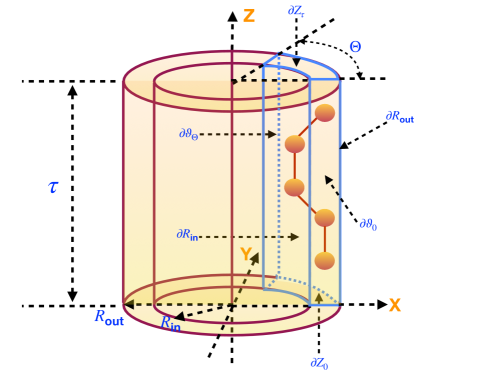
Figure 3: Illustration of the simulation domain $\Omega$ (domain boundary lines in blue) for an untwisted helical structure (i.e., $\alpha=0$). A few atoms contained in the domain, as well as the various bounding surfaces of the domain are illustrated. For a structure associated with a two-generator helical group, the parameter $\Theta=2\pi/\mathfrak{N}$ relates to the cyclic group order, while $\tau$ is related to the pitch of the screw transformation.

We set up a finite difference grid over $\Omega$ using helical coordinates, with spacing $h_{r}$, $h_{\theta_{1}}$ and $h_{\theta_{2}}$ along the $r$, $\theta_{1}$ and $\theta_{2}$ directions respectively. Since the simulation domain can be represented in helical coordinates with $r$ ranging from $R_{\text{in}}$ to $R_{\text{out}}$, $\theta_{1}$ ranging from $0$ to $1$, and $\theta_{2}$ ranging from $0$ to $\frac{1}{\mathfrak{N}}$, it follows that $R_{\text{out}}-R_{\text{in}}=\mathscr{N}_{r}h_{r}$, $1=\mathscr{N}_{\theta_{1}}h_{\theta_{1}}$, and $\frac{1}{\mathfrak{N}}=\mathscr{N}_{\theta_{2}}h_{\theta_{2}}$, for natural numbers $\mathscr{N}_{r}$, $\mathscr{N}_{\theta_{1}}$ and $\mathscr{N}_{\theta_{2}}$. We index the finite difference nodes using a triplet of natural numbers $(\mathsf{i},\mathsf{j},\mathsf{k})$, for $\mathsf{i}=1,2,\ldots,\mathscr{N}_{r}$, $\mathsf{j}=1,2,\ldots,\mathscr{N}_{\theta_{1}}$ and $\mathsf{k}=1,2,\ldots,\mathscr{N}_{\theta_{2}}$. We denote the value of a function $f$ at the grid point $(\mathsf{i},\mathsf{j},\mathsf{k})$ as $f^{(\mathsf{i},\mathsf{j},\mathsf{k})}$. We will denote $h=\text{Max.}\bigg{(}h_{r},\tau h_{\theta_{1}},\big{(}\frac{R_{\text{in}}+R_{\text{out}}}{2}\big{)}h_{\theta_{2}}\bigg{)}$ as the mesh spacing.

The formulae presented in Section 2.2.2 and C require Cartesian gradients, the Laplacian operator and integrals over $\Omega$ to be evaluated using the finite difference scheme. The formulae for these quantities, as expressed in helical coordinates appears in D. With these in hand, we approximate the first order partial derivatives using central differences as:

$$\frac{\partial f}{\partial r}\bigg{|}^{(\mathsf{i},\mathsf{j},\mathsf{k})} \approx\sum_{p=1}^{n_{o}}\bigg{(}{w}_{p,r}^{\text{first}}\big{(}f^{(\mathsf{i}+p,\mathsf{j},\mathsf{k})}-f^{(\mathsf{i}-p,\mathsf{j},\mathsf{k})}\big{)}\bigg{)}\,,$$

$$\frac{\partial f}{\partial\theta_{1}}\bigg{|}^{(\mathsf{i},\mathsf{j},\mathsf{k})} \approx\sum_{p=1}^{n_{o}}\bigg{(}{w}_{p,\theta_{1}}^{\text{first}}\big{(}f^{(\mathsf{i},\mathsf{j}+p,\mathsf{k})}-f^{(\mathsf{i},\mathsf{j}-p,\mathsf{k})}\big{)}\bigg{)}\,,$$

$$\frac{\partial f}{\partial\theta_{2}}\bigg{|}^{(\mathsf{i},\mathsf{j},\mathsf{k})} \approx\sum_{p=1}^{n_{o}}\bigg{(}{w}_{p,\theta_{2}}^{\text{first}}\big{(}f^{(\mathsf{i},\mathsf{j},\mathsf{k}+p)}-f^{(\mathsf{i},\mathsf{j},\mathsf{k}-p)}\big{)}\bigg{)}\,.$$ (126)

We approximate the pure (i.e., non-mixed) second order partial derivatives as:

$$\frac{\partial^{2}f}{\partial r^{2}}\bigg{|}^{(\mathsf{i},\mathsf{j},\mathsf{k})} \approx\sum_{p=0}^{n_{o}}\bigg{(}{w}_{p,r}^{\text{second}}\big{(}f^{(\mathsf{i}+p,\mathsf{j},\mathsf{k})}+f^{(\mathsf{i}-p,\mathsf{j},\mathsf{k})}\big{)}\bigg{)}\,,$$

$$\frac{\partial^{2}f}{\partial\theta_{1}^{2}}\bigg{|}^{(\mathsf{i},\mathsf{j},\mathsf{k})} \approx\sum_{p=0}^{n_{o}}\bigg{(}{w}_{p,\theta_{1}}^{\text{second}}\big{(}f^{(\mathsf{i},\mathsf{j}+p,\mathsf{k})}+f^{(\mathsf{i},\mathsf{j}-p,\mathsf{k})}\big{)}\bigg{)}\,,$$

$$\frac{\partial^{2}f}{\partial\theta_{2}^{2}}\bigg{|}^{(\mathsf{i},\mathsf{j},\mathsf{k})} \approx\sum_{p=0}^{n_{o}}\bigg{(}{w}_{p,\theta_{2}}^{\text{second}}\big{(}f^{(\mathsf{i},\mathsf{j},\mathsf{k}+p)}+f^{(\mathsf{i},\mathsf{j},\mathsf{k}-p)}\big{)}\bigg{)}\,,$$ (127)

while the mixed second order partial derivative $\displaystyle\frac{\partial^{2}f}{\partial\theta_{1}\partial\theta_{2}}$ is obtained by applying the above first order derivative formula first in $\theta_{1}$ and then in $\theta_{2}$, i.e.,

$$\frac{\partial^{2}f}{\partial\theta_{1}\partial\theta_{2}}\bigg{|}^{(\mathsf{i},\mathsf{j},\mathsf{k})} \approx\sum_{p=1}^{n_{o}}{w}_{p,\theta_{2}}^{\text{first}}\bigg{[}\bigg{(}\frac{\partial f}{\partial\theta_{1}}\bigg{)}^{(\mathsf{i},\mathsf{j},\mathsf{k}+p)}-\bigg{(}\frac{\partial f}{\partial\theta_{1}}\bigg{)}^{(\mathsf{i},\mathsf{j},\mathsf{k}-p)}\bigg{]}\,$$

$$\approx\sum_{p=1}^{n_{o}}{w}_{p,\theta_{2}}^{\text{first}}\bigg{[}\bigg{\{}\sum_{p^{\prime}=1}^{n_{o}}{w}_{p^{\prime},\theta_{1}}^{\text{first}}\big{(}f^{(\mathsf{i},\mathsf{j}+p^{\prime},\mathsf{k}+p)}-f^{(\mathsf{i},\mathsf{j}-p^{\prime},\mathsf{k}+p)}\big{)}\bigg{\}}$$

$$\quad\quad\quad\quad\;\,-\bigg{\{}\sum_{p^{\prime}=1}^{n_{o}}{w}_{p^{\prime},\theta_{1}}^{\text{first}}\big{(}f^{(\mathsf{i},\mathsf{j}+p^{\prime},\mathsf{k}-p)}-f^{(\mathsf{i},\mathsf{j}-p^{\prime},\mathsf{k}-p)}\big{)}\bigg{\}}\bigg{]}$$ (128)

In the above formulae, $n_{o}$ denotes half the finite difference order and is set to $6$ for all our simulations (i.e., $12^{\text{th}}$ order finite differences are used). This choice has also been employed elsewhere [33, 34, 40, 63] and is found to be adequate for attaining chemical accuracy. Letting $s$ denote $r$, $\theta_{1}$ or $\theta_{2}$, the weights that appear in the above formulae can be expressed as [128]:

$$w_{0,s}^{\text{second}} =-\frac{1}{h_{s}^{2}}\sum_{q=1}^{n_{o}}\frac{1}{q^{2}}\,,\,\,$$

$$w_{p,s}^{\text{second}} =\frac{2(-1)^{p+1}}{h_{s}^{2}\,p^{2}}\frac{(n_{o}!)^{2}}{(n_{o}-p)!(n_{o}+p)!}\,\,\text{for}\,\,p=1,2,\ldots,n_{o}\,,$$

$${w}_{p,s}^{\text{first}} =\frac{(-1)^{p+1}}{h_{s}\,p}\frac{(n_{o}!)^{2}}{(n_{o}-p)!(n_{o}+p)!}\,\,\text{for}\,\,p=1,2,\ldots,n_{o}\,.$$ (129)

We employ the following quadrature rule for approximating integrals over $\Omega$:

$$\int_{\Omega}f({\bf x})\,d{\bf x}\approx h_{r}h_{\theta_{1}}h_{\theta_{2}}\sum_{\mathsf{i}=1}^{\mathscr{N}_{r}}\sum_{\mathsf{j}=1}^{\mathscr{N}_{\theta_{1}}}\sum_{\mathsf{k}=1}^{\mathscr{N}_{\theta_{2}}}2\pi\tau r_{\mathsf{i}}\,f^{(\mathsf{i},\mathsf{j},\mathsf{k})}\,,$$ (130)

with $r_{\mathsf{i}}$ denoting the radial coordinate of the finite difference node $(\mathsf{i},\mathsf{j},\mathsf{k})$.

3.5 Boundary conditions

We need to specify the boundary conditions on the various fields that are being solved for in the governing equations. These are the helical Bloch states $\psi_{j}({\bf x};\eta,\nu)$ (for $\eta\in\mathfrak{I}$ and $\nu=\{0,1,2,\ldots,\mathfrak{N}-1\}$) which satisfy the Kohn-Sham equations (eq. 109 or eq. 193), and the total electrostatic potential $\Phi$ which satisfies Poisson’s equation (eq. 111 or eq. 198). In helical coordinates, we may interpret the helical Bloch boundary conditions (eq. 179) as the following conditions:

$$\psi_{j}(r,\theta_{1}=1,\theta_{2};\eta,\nu)=e^{-i2\pi\eta}\psi_{j}(r,\theta_{1}=0,\theta_{2};\eta,\nu)\,,$$ (131)

which applies to the surfaces $\partial Z_{0}\bigcup\partial Z_{\tau}$; as well as the condition:

$$\psi_{j}(r,\theta_{1},\theta_{2}=\frac{1}{\mathfrak{N}};\eta,\nu)=e^{-i2\pi\frac{\nu}{\mathfrak{N}}}\psi_{j}(r,\theta_{1},\theta_{2}=0;\eta,\nu)\,,$$ (132)

which applies to the surfaces $\partial\vartheta_{0}\bigcup\partial\vartheta_{\Theta}$. We assume that the atoms within $\Omega$ are sufficiently far away from the boundary surfaces $\partial R_{\text{in}}$ and $\partial R_{\text{out}}$, so that the electron density decays to zero at these surfaces and zero Dirichlet boundary conditions on the wavefunctions (Section 2.2.1) can be applied. Thus, the conditions to be applied on the surfaces $\partial R_{\text{in}}\bigcup\partial R_{\text{out}}$ are:

$$\psi_{j}(r=R_{\text{in}},\theta_{1},\theta_{2};\eta,\nu)=\psi_{j}(r=R_{\text{out}},\theta_{1},\theta_{2};\eta,\nu)=0\,.$$ (133)

As already discussed, the electrostatic potential $\Phi$ inherits the symmetry of the helical structure (i.e., it is invariant under ${\cal G}_{1}$ or ${\cal G}_{2}$). Thus, it follows that the boundary conditions on this quantity on the surfaces $\partial Z_{0}\bigcup\partial Z_{\tau}$ and $\partial\vartheta_{0}\bigcup\partial\vartheta_{\Theta}$ are respectively:

$$\Phi(r,\theta_{1}=1,\theta_{2})=\Phi(r,\theta_{1}=0,\theta_{2})\,,$$

$$\Phi(r,\theta_{1},\theta_{2}=\frac{1}{\mathfrak{N}})=\Phi(r,\theta_{1},\theta_{2}=0)\,.$$ (134)

To apply the right boundary conditions on $\Phi$ on the surfaces $\partial R_{\text{in}}\bigcup\partial R_{\text{out}}$, we may evaluate eq. 99 or eq. 191 directly using Ewald summation [74] or multipole expansion [91] techniques.

3.6 Numerical linear algebra issues

On every SCF iteration step, the lowest $N_{\text{s}}$ eigenstates of a set of $N_{\mathcal{K}}$ Kohn-Sham operators (indexed by $\eta_{b}$ for the case of ${\cal G}_{1}$, and $\eta_{b},\nu$ for the case of ${\cal G}_{2}$) have to be computed. We employ iterative diagonalization based on Chebyshev polynomial filtered subspace iterations (CheFSI) [129, 130, 131, 132] for this purpose. Due to the fact that the helical coordinate system is curvilinear, the finite difference discretization of the Laplacian operator results in a discretized operator that is non-Hermitian (even though the Laplacian as an operator on an infinite dimensional Hilbert space is Hermitian). This results in the discretized Hamiltonian operator also being non-Hermitian, which can lead to non-real eigenvalues of the matrix. However, as the discretization is made finer (i.e., $h_{r},h_{\theta_{1}},h_{\theta_{2}}$ become smaller) the discretized Laplacian and Hamiltonian matrices approach Hermitian matrices and so, the eigenvalues resulting from these discretized operators tend to have vanishingly small imaginary parts [133, 40]. In practice, for the mesh spacings that have been considered in this work, the imaginary parts are small enough that they can be safely ignored without affecting the quality of the simulations (also see [40] and [63] where a similar situation was encountered).

We use Chebyshev polynomial filter orders in the range $55$ to $80$ for our simulations. This is somewhat higher than what is commonly employed in finite difference DFT calculations in affine coordinate systems with comparable mesh spacing [130, 33, 34]. We adopt it here to mitigate the effect of the larger spectral width of the discretized Hamiltonian that arises due to crowding of grid points as one approaches the origin in helical coordinates. We have also observed that the time for computing matrix-vector products using the discretized Hamiltonian in helical coordinates is larger compared to the time required for the case of a finite difference Hamitonian (of the same size) arising from a cylindrical system (obtained by setting the twist angle parameter $\alpha$ to $0$ in the helical case). This is certainly due to the presence of cross derivatives in the helical case (eq. 128), which makes the discretized Hamiltonian somewhat less sparse when compared with the cylindrical one. Within the CheFSI method, we use Arnoldi iterations for computing the extremal eigenvalues of the Hamiltonian and a direct diagonalization method for computing the projected subspace problem.

We use the Generalized Minimal Residual method (GMRES) [134] to solve the Poisson problem associated with the total electrostatic potential $\Phi$. To accelerate convergence, we use an incomplete LU factorization based preconditioner [135].

3.7 Matlab implementation: The Helical DFT code

We have implemented the above computational strategies using the MATLAB [136] software package into a code called Helical DFT. The code parallelizes computation over the different $\eta$ and $\nu$ values using MATLAB’s Parallel Computing Toolbox (the parfor function). For maximum efficiency of the MATLAB implementation, code vectorization has been used as much as possible. However, for computing certain quantities (such as the atomic forces and the net nuclear pseudocharge), multiple levels of nested loops were found unavoidable. These routines were converted into machine code by use of the MATLAB Coder framework, which helped alleviate performance issues. In order to reduce the memory footprint associated with the storage of the different Hamiltonian matrices arising from the $N_{{\cal K}}$ different values of $\eta_{b}$ (and also $\nu$ for ${\cal G}_{2}$), we avoid computing matrix vector products through MATLAB’s internal sparse matrix framework since that requires these matrices to be available explicitly. Instead, we store only the Laplacian part of the Hamiltonian matrix in compressed sparse row (CSR) format and apply the helical Bloch boundary conditions associated with the different values of $\eta_{b}$ and/or $\nu$ on the fly, while computing matrix vector products. The actual task of computing these matrix vector products is carried out using a C language routine which has been compiled and interfaced with our MATLAB code.

Some other relevant details related to the implementation are as follows. We use the periodic variant of Pulay’s scheme [137, 138] in the total potential to accelerate the convergence of the SCF iterations. The Fermi energy is calculated using a nonlinear equation root finder (MATLAB’s fzero function). When required, structural relaxation is achieved by an implementation of the Fast Intertial Relaxation Engine (FIRE) algorithm [139].

4 Simulation Results and Discussion

We now turn to a discussion of numerical simulations and results. All simulations were run using a single node of the Mesabi cluster at the Minnesota Supercomputing Institute, or a single node of the Hoffman2 cluster at UCLA’s Institute for Digital Research and Education. Each compute node of Mesabi has $24$ Intel Haswell E5-2680v3 processors operating at $2.50$ GHz, and $64$ GB to $1$ TB of RAM. Each compute node of the Hoffman2 cluster has two $18$-core Intel Xeon Gold 6140 processors (with $24.75$ MB cache, and running at $2.3$ GHz), and $192$ GB of RAM.

All calculations presented here use Troullier-Martins norm conserving pseudopotentials [113]. The Local Density Approximation [25] was used for modeling the exchange correlation energy, and the Perdew-Wang parametrization [140] of the correlation energy was employed. An electronic temperature of $T_{\text{e}}=315.77$ Kelvin was used for Fermi-Dirac smearing to help accelerate SCF convergence.

The large majority of the simulations here have focused on the study of single wall nanotubes. Starting from the sheet of an elemental two-dimensional material, nanotubes of any chirality can be formed using the so-called “roll-up” construction [141]. This procedure also allows us to see [7, 49] that such nanotubes can be adequately represented using helical groups generated by two elements with just $4$ atoms in the fundamental domain [63]. In this representation, the twist angle parameter $\alpha$ becomes related to the chirality of the tubes ($\alpha=0$ for achiral tubes), while the parameter $\mathfrak{N}$, associated with the cyclic group order, is related to the tube radius [49]. In our nanotube simulations, we have ensured that the atoms within the fundamental domain are always located $10$ to $12$ Bohrs away from the boundary surfaces $\partial R_{\text{in}}$ and $\partial R_{\text{out}}$ so as to allow sufficient decay of the electron density and the wavefunctions in the radial direction.

4.1 Materials system: Single layer black phosphorus nanotubes

Single-layer black phosphorus, or phosporene, is a two-dimensional nanomaterial that has been the object of intense investigation in recent years due its association with a number of unusual and fascinating material properties [142, 143, 144, 145, 146, 147, 148]. Nanotubes of this material, as formed by the roll-up construction have also received attention in the literature [149, 150, 151, 152, 153, 154, 155, 156, 157, 158, 159, 160, 161, 162], due to their interesting optical and electronic properties, and the coupling of these properties to mechanical strains. This motivates our choice in selecting this material for the simulations presented in this work.

As a starting point, we obtained the ground state structure of a single layer of phosphorene (Figure 4) using the same pseudopotential, exchange correlation functional and electronic temperature as the Helical DFT simulations subsequently described. We used the plane-wave DFT code ABINIT [30, 163] to perform the geometry relaxation calculation. The periodic unit cell for this simulation contained $4$ atoms. An energy cutoff of $40$ Ha, along with $30\times 30\times 1$ k-points and a cell vacuum of $25$ Bohr in the Z-direction was used. At the end of this very refined calculation the atomic forces were all less than $10^{-5}$ Ha/Bohr, while the cell stresses were of the order of $10^{-8}\;\text{Ha/Bohr}^{3}$ or lower. Some of the structural parameters obtained from the calculation are shown in Table 1. There appears to be generally good agreement with the literature thus giving us confidence in the reliability of the subsequent simulations with regard to materials physics.

Lattice constant $a_{1}$	Lattice constant $a_{2}$	Bond length $\delta_{1}$	Bond length $\delta_{2}$	Bond angle $\gamma$
along X axis (Å)	along Y axis (Å)	(Å)	(Å)	(degrees)
$3.26$	$4.36$	$2.20$	$2.193$	$102.42$
($3.35$ [145], $3.3$ [165])	($4.62$ [145], $4.5$ [165])	($2.29$ [165])	($2.25$ [165])	($103.3$ [165])

Table 1: Structural parameters of phosphorene computed using a periodic DFT calculation. Quantities in parentheses refer to values in the literature along with references. Explanation of the parameters is available from Figure 4

.

(a) Top view of a phosphorene sheet. Atoms in the shaded region are placed in the Helical DFT simulation cell (fundamental domain).

(b) Side view of a phosphorene sheet. Different structural parameters are labeled. Values available in Table 1.

Figure 4: Phosphorene lattice as computed using a periodic DFT calculation. This provides the starting point for Helical DFT calculations involving phosphorene nanotubes. For zigzag tubes, the parameter $\tau$ in the two-generator helical group is set to be equal to the lattice constant $a_{2}$ along the Y-axis.

To represent the zigzag phosphorene nanotubes in the Helical DFT simulations described next, we roll up the phosphorene sheet along the X-axis and place the atoms from the aforementioned periodic unit cell (the shaded region in Figure 4) into the Helical DFT simulation cell ($\Omega$). In the absence of relaxation effects, the pitch $\tau$ associated with the two-generator helical group, is equal to the lattice constant along the Y axis. Furthermore, the angle $\Theta$ associated with the cyclic group order $\mathfrak{N}$ is related to the radius of the nanotube via the relation $\displaystyle\Theta=\frac{2\pi}{\mathfrak{N}}=\frac{a_{1}}{R_{\text{avg.}}}$. Here $a_{1}$ denotes the lattice vector along the X-axis in the phosphorene sheet, and $R_{\text{avg.}}$ denotes the average radial coordinate of the atoms in the fundamental domain of the nanotube. For chiral nanotubes, we additionally include a no-zero twist angle parameter $\alpha$. Figure 5 shows examples of two phosphorene nanotubes studied in this work using Helical DFT.

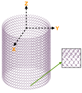
(a) Zigzag phosphorene nanotube.

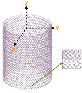
(b) Chiral phosphorene nanotube obtained by setting the angle of twist parameter $\alpha=0.005$.

Figure 5: Representative phosphorene nanotubes (radius = $3.4$ nanometers) studied in this work using Helical DFT. Insets show zoomed-in views of the atomic arrangement to highlight differences between the two cases.

4.2 Convergence and accuracy

To study the convergence properties of our numerical implementation, we consider a chiral phosphorene nanotube of radius $1.76$ nanometers. The cyclic group order is $\mathfrak{N}=32$ and the twist angle parameter is $\alpha=0.0025$. For a given structure and a fixed simulation domain, the two convergence parameters under study are the mesh spacing $h=\text{Max.}\bigg{(}h_{r},\tau h_{\theta_{1}},\big{(}\frac{R_{\text{in}}+R_{\text{out}}}{2}\big{)}h_{\theta_{2}}\bigg{)}$, and the number of points $N_{\eta}$ used for discretizing the set $\mathfrak{I}$ in reciprocal space. As a reference calculation, we computed the electronic structure of the system with the finest mesh ($h=0.23$ Bohr) and the highest value of $N_{\eta}$ ($=23$) that we could afford under computational resource constraints. First, for the mesh convergence study, we fix $N_{\eta}=23$ and carry out a series of calculations with $h\approx 0.30,0.40,0.50,0.60,0.65,0.70$ Bohr. Next, for studying convergence with respect to $N_{\eta}$, we fix $h=0.23$ Bohr and carry out a series of calculations with $N_{\eta}=1,3,7,11,15,19$. We plot the errors in the energy per atom and the atomic forces in each of the above cases in Figure 6.

From the figures, it is clear that the code converges to the reference calculations systematically. Using straight-line fits to the convergence data with respect to $h$, we find slopes of $5.8$ and $7.6$ for the energies and forces, respectively. These numbers are very nearly identical to the convergence rates observed in finite difference calculations involving cylindrical coordinates [63] and are also comparable to finite difference calculations in affine coordinate systems [33, 34]. From the data, we are also able to estimate that the parameters $h=0.40$ Bohr and $N_{\eta}=11$ are more than sufficient to reach chemically accurate energies and forces (the exact errors for these choices with respect to the reference calculation were $2\times 10^{-4}$ Ha/atom and $8\times 10^{-5}$ Ha/Bohr in the energies and forces, respectively). For computational efficiency therefore, we use this set of parameters for all relaxation calculations described subsequently, and switch to the reference calculation parameters (i.e., $h=0.23$ Bohr, $N_{\eta}=23$) only when more accurate energies / band gaps are required at the end of a relaxation procedure.

Verifying the accuracy of the Helical DFT code with respect to standard plane-wave codes can be challenging since the plane-wave codes may be required to include an enormous number of atoms in the periodic unit cell in order to replicate the exact system being studied by Helical DFT. In case of the above chiral nanotube system for example, over $50,000$ atoms would be needed, making the planewave calculation unfeasible. Therefore, we carry out this accuracy check in two steps. First, we set up a Helical DFT calculation for a zigzag nanotube (i.e., $\alpha=0$) of radius $0.94$ nanometers. For this tube, the cyclic group order $\mathfrak{N}=16$. Then, we simulate this tube using the ABINIT code by employing a $64$ atom unit cell (periodicity was enforced along the Z axis, Dirichlet boundary conditions were enforced along X and Y axes by padding with a large amount of vacuum). We converged both codes to the extent allowed by computational resources, and observed that the energies (in Ha/atom) and the forces (in Ha/Bohr) from these two calculations agreed with each other to $1\times 10^{-4}$ or better. Next to study a case for which $\alpha\neq 0$, we set up an artificial system consisting of atoms along a single helix (similar to the configuration in Figure 2). This system was generated using a single generator helical group ($\mathfrak{N}=1$) and used $\alpha=0.01$. The helical unit cell had $2$ atoms, while the periodic unit cell in ABINIT involved $200$. Once again, upon convergence with respect to their respective discretization parameters, the codes produced results that differed from each other by about $1\times 10^{-4}$ Ha/atom or Ha/Bohr. This completes the accuracy tests.

Through the above examples, we were also able to observe that for realistic helical nanostructure simulations, the wall time for Helical DFT can be up to orders of magnitude smaller compared to a well optimized plane-wave code like ABINIT, making it a powerful first principles tool in the study of such systems.

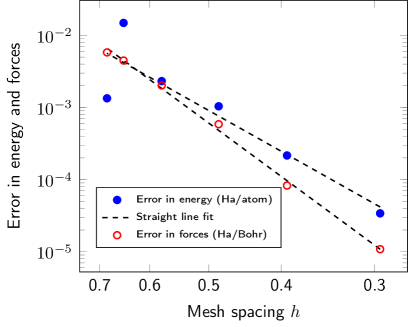
(a) Convergence with respect to discretization in real space.

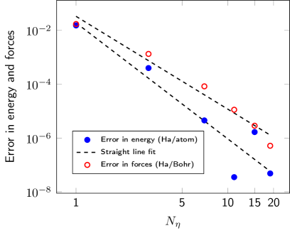
(b) Convergence with respect to number of points used to discretize $\mathfrak{I}$.

 

Figure 6: Convergence properties of the Helical DFT code with respect mesh size $h$ and the number of points $N_{\eta}$ used to discretize the set $\mathfrak{I}$. The error in the forces is computed by considering the magnitude of the maximum difference in all the force components of all the atoms.

4.3 Simulation of twisting: Ab initio computation of torsional stiffness

By using the two-generator helical group ${\cal G}_{2},$ it is possible to describe torsional deformations in nanostructures [49, 166, 167, 168, 55]. We use this procedure here to illustrate the utility of Helical DFT in extracting mechanical properties of nanomaterials ab initio. Specifically, we investigate the behavior of a zigzag phosphorene nanotube (nanotube radius $3.4$ nanometer, cyclic group order $\mathfrak{N}=64$.) under twisting deformations. We begin with the untwisted structure ($\alpha=0$) and relax the atoms in the simulation cell till all force components on all atoms are below $10^{-3}$ Ha/Bohr. Starting from this relaxed structure, we apply twisting deformations to the nanotube by prescribing non-zero values of the twist angle parameter $\alpha$ in the two-generator helical group ${\cal G}_{2}$ used for describing the nanotubes. We varied $\alpha$ in steps of $0.001$ and relaxed the resulting nanotube structure in each case, till all components of the forces on all the atoms in the simulation cell dropped below $10^{-3}$ Ha/Bohr once again. The largest twist we considered is about $5$ degrees per nanometer length of the tube, which corresponds to $\alpha=0.006$. Anticipating a quadratic dependence of the nanotube twist energy for small values of alpha [49], we plot the results as shown in Figure 7. In that figure, we have also plotted the twisting energies obtained when the atomic relaxation effects are not considered.

We write the twist energy per unit length of the tube as $U_{\text{twist}}=\frac{1}{2}k_{\text{twist}}\,\beta^{2}$, with $\beta$ denoting the twist per unit length of the tube ($\beta=\frac{2\pi\alpha}{\tau}$) and $k_{\text{twist}}$ denoting the torsional stiffness. From the figure, we use the straight line fits near zero twist to estimate the value of $k_{\text{twist}}$ as $13.66$ eV nm $\text{(deg)}^{-2}$ and $27.33$ eV nm $\text{(deg)}^{-2}$, for the relaxed and unrelaxed cases respectively. It is also evident from the figure that non-linear effects start to play a noticeable role in this nanotube at around $4$ degrees of twist per nanometer. These simulations serve as an example of determining constitutive parameters directly from quantum mechanics using Helical DFT.

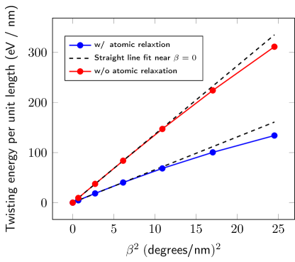
(a)

Figure 7: Twist energy of a zigzag phosphorene nanotube as obtained via Helical DFT.

4.4 Electronic properties: Behavior of zigzag tubes under torsional deformations

Since Helical DFT is an ab initio simulation tool, it can give us insights into the electronic, optical and transport properties of materials under study. In particular, it may be used to shed light into the coupling of mechanical strains with these properties. To illustrate these points, we consider again the case of the zigzag phosphorene nanotube discussed above (nanotube radius $3.4$ nanometer, cyclic group order $\mathfrak{N}=64$.). Figure 8 displays examples of helical band structure diagrams, which like their periodic counterparts, can be used to illustrate the electronic levels in the system. A unique feature of these diagrams however, is that they can be used to display the variation of Kohn-Sham eigenvalues with respect to $\eta$ and $\nu$. This makes them significantly easier to interpret than traditional periodic band diagrams for quasi-one-dimesional (nanotube-like) structures, which have only one index (i.e., the wave vector $k_{z}$ in the axial direction) labeling the Kohn-Sham states. We anticipate that helical band diagrams like the ones shown are likely to emerge as powerful tools in understanding instabilities in optical and electronic materials.

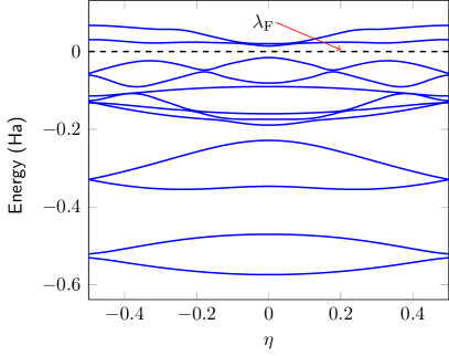
(a) Helical band diagram in $\eta$, along $\nu=0$.

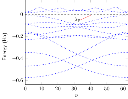
(b) Helical band diagram in $\nu$, along $\eta=0$.

 

Figure 8: Helical band structure diagrams for an untwisted zigzag phosphorene nanotube (radius $=3.4$ nanometers). $\lambda_{\text{F}}$ denotes the Fermi level (shifted to $0$).

The helical band diagrams described above can be used to compute the size of the band gap of the system and infer whether it is conducting, semiconducting or insulating. We plot in Figure 9 the variation in the band gap of the above nanotube, as it undergoes torsional deformations. The variation with and without atomic relaxation effects are both displayed. From the figure, we observe that the nanotube has a semiconducting behavior overall, and can be made to go from an insulating state at no twist (direct band gap of about $0.81$ eV), to a practically conducting one, once the twist reaches about $5$ degrees per nanometer. This is a rather significant change in the electronic properties of the material, although in a mechanical sense, its deviation from simple linear elastic behavior (Figure 7) is still fairly modest at this level of twist.

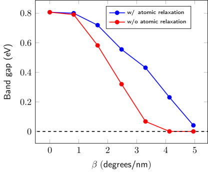
(a)

Figure 9: Effect of torsional deformation on the band gap of a zigzag phosphorene nanotube (radius $=3.4$ nanometers).

To further illustrate the above electronic transition, we compute the (electronic) density of states of the nanotube without and with twist ($\beta\approx 5$ degrees/nanometer). Following [44], we write this at a given energy level $E$ and an electronic temperature of $T_{\text{e}}$ as:

$$\aleph_{T_{\text{e}}}(E)=2\,\int_{\mathfrak{I}}\frac{1}{\mathfrak{N}}\sum_{\nu=0}^{\mathfrak{N}-1}\bigg{(}\sum_{j=1}^{\infty}f^{\prime}_{T_{\text{e}}}\big{(}E-\lambda_{j}(\eta,\nu)\big{)}\bigg{)}\,d\eta,$$ (135)

and evaluate it along a fine mesh of values of $E$ in the range $[-1,1]$. The results are shown in Figure 10. It is apparent from the figure that the electronic states in the system undergo significant change as the nanotube is subjected to twisting. In particular, the number of states at or near the Fermi level $\lambda_{\text{F}}$, increases to values well above $0$, indicating onset of metallic behavior when the tube is twisted.

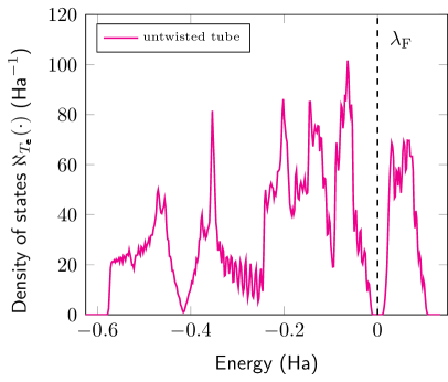
(a) Density of states of untwisted nanotube.

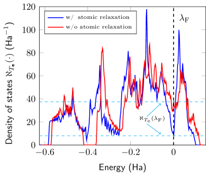
(b) Density of states of twisted nanotube.

Figure 10: Electronic density of states plot for a zigzag phosphorene nanotube (radius $=3.4$ nanometers), without and with twist. $\lambda_{\text{F}}$ denotes the Fermi level (shifted to $0$).

4.5 Electronic properties: Behavior of chiral tubes under axial strains

Finally, we use Helical DFT to study a chiral phosphorene nanotube. We choose a tube with $\mathfrak{N}=64$ and $\tau=8.244$ Bohr as before, and also set $\alpha=0.005$. We relax the positions of the atoms within the simulation cell and use the resulting nanotube (observed to have an indirect band gap of about $0.24$ eV) as the starting structure for subsequent simulations. We subject this tube to (both tensile and compressive) axial strains by varying $\tau$, and relax the atomic positions in each case. Figure 11 shows the variation in the band gap of this tube at different values of axial strain. The effect of not including atomic relaxation after the tube is subjected to the strains is also shown.

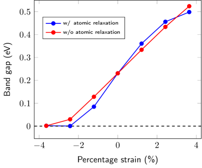
(a)

Figure 11: Effect of axial strain on the band gap of a chiral phosphorene nanotube ($\mathfrak{N}=64$, $\alpha=0.005$).

From the figure, we see that in the range of strains considered, compressive strains tend to reduce the band gap, while tensile strains appear to increase it. The tube appears to transition into a metallic state at about $4\%$ compressive strain. Based on the nature of the plot and motivated by earlier work on chiral carbon nanotubes [182, 183], we fitted a one-term Fourier series to this band gap data, and found that this produces a high quality fit for both the relaxed and unrelaxed cases. This suggests that like the case of carbon nanotubes, it might be possible to build (approximate) tight-binding type models of the band gap behavior [184] for phosphorene nanotubes. This is a topic that warrants further investigation. Notably, the parameters in such models can be provided through high-quality ab initio simulations based on Helical DFT.

The above ab initio simulations of the phosphorene nanotubes (both zigzag and chiral) suggests that these materials have highly adjustable electronic states. Therefore, they might find future applications as nanomaterials with tunable electronic/optical/transport properties. The simulations also highlight the possibility of using inhomogeneous strain modes for altering these properties, instead of homogeneous strain modes which are considered in the strain-engineering literature [185, 186, 187] more commonly. Further investigations of this material and others, along these lines, is the scope of future work.

Finally, we find it worthwhile to point out that the phosphorene nanotube simulations described above (both electronic and mechanical) would be very challenging, or well-nigh impossible to carry out using conventional first principles techniques, even with the aid of massively parallel high-performance computing resources. In contrast, our MATLAB implementation of Helical DFT often allows such simulations to be carried out within a few hours of simulation wall time on a desktop workstation or a single node of a supercomputing cluster, thus serving to reinforce the novelty and practical utility of the approach.

5 Conclusions and Future Directions

In summary, we have presented Helical DFT — a novel, systematic first principles simulation framework for systems with helical symmetries. We have presented a derivation of the equations of Kohn-Sham theory, as they apply to the case of helical structures. Our derivation is systematic, self-contained and for the most part, mathematically rigorous. We have then solved these governing equations numerically by using a finite difference method based on helical coordinates. Using this working realization of the proposed approach, we have carried out simulations involving phosphorene nanotubes, extracted their mechanical behavior ab initio, and identified changes in the electronic properties of this material as it undergoes twisting.

Having laid out this foundational work on Helical DFT, we now discuss a number of avenues for future investigation:

• Development of an efficient spectral solution scheme: While the current finite difference based implementation of Helical DFT allows us to investigate a number of materials systems of interest, it also suffers a number of computational deficiencies (Section 3). Following our earlier work on the ab initio simulations of cluster systems with arbitrary point group symmetries, we have already formulated, and are currently in the process of implementing a spectral scheme for solving the governing equations [8, 188, 46]. This is expected to completely resolve the issues with the finite difference formulation and provide a more efficient numerical implementation, thus opening the door to the simulation of more complex helical structures.

• Mechanistic simulations of quasi-one-dimensional systems: The materials science literature is rich with examples of quasi-one-dimensional structures that have been discovered and/or synthesized through experimental means. The simulation tools developed here can be used to characterize these materials computationally. In particular, the use of helical symmetry adapted ab initio molecular dynamics [189] can be used to study the mechanical behavior of these materials under axial and torsional strains, as well as their instabilities and defects [190, 49, 51].

• Helical Wannier states and the helical Berry phase: The helical Bloch Floquet transform ${\cal U}$ introduced in eqs. 38 and 180 allows us to consider the notion of helical Wannier states. These, like their periodic counterparts, are defined through the action of ${\cal U}^{-1}$ on the helical Bloch states [85], and can be expected to be exponentially localized for insulating systems [191]. Additionally, like the case of periodic systems, a geometric phase (i.e., the Berry phase [192]) associated with the helical Bloch phase factor may be defined. These observations are likely to spur the development of novel computational analysis methods [193, 194] for helical materials, as well as the discovery of novel topological materials [195, 196].

• Search for exotic materials properties and study of multi-physics coupling: Since Helical DFT is a first principles simulation technique, it allows investigation of the effect of torsional deformations on a material’s optical, electronic, magnetic and transport properties. Like the case of the phospherene nanotube considered in this work, it is possible that torsional or axial deformations in certain helical structures might induce a significant redistribution of electronic states in the material, leading to the appearance of interesting collective properties. In this regard, the investigation of the nanoscale flexoelectric effect [197, 198, 199, 200, 201, 202] in helical systems would be of particular interest, since owing to the quasi-one-dimensional nature of these materials, as well as the appearance of strain gradients in connection with torsional deformations, a significant polarization may appear along the axis of a nanostructure when twisted, thus leading to a strong flexoelectric effect.

• Search for new phases of matter and coherent phase transformations: Finally, as remarked in [71, 70], the first principles techniques developed here might be instrumental in the discovery of novel phases of matter. Additionally, the discovery of transformations between such phases [70, 203] — particularly, coherent ones [204, 205] — are likely to lead to new classes of active materials. The methods developed here are likely to be very useful in the characterization of energy barriers of such transformations and help in their design.

—

Appendix A Verifying that the operator $\mathfrak{h}_{\eta}^{\textsf{aux}}$ in Eq. 25 is symmetric

The boundary conditions associated with the operator $\mathfrak{h}^{\textsf{aux}}_{\eta}$ introduced in Eq. 25 are quite non-conventional. Here, we work through the steps of verifying that the operator is symmetric when augmented with these boundary conditions. For this, we consider smooth functions $f_{1},f_{2}$ over ${\cal D}$ (the interior of the fundamental domain ${\cal D}_{{\cal G}_{1}}$), obeying the same boundary conditions as $\phi$ in the proof of Theorem 2.3, i.e., $f_{1,2}({\bf x})=f_{1,2}(\Upsilon_{\mathsf{h}}\circ{\bf x})$, $\nabla f_{1,2}({\bf x})={\bf R}_{2\pi\alpha}^{-1}\nabla f_{1,2}(\Upsilon_{\mathsf{h}}\circ{\bf x})$ for ${\bf x}\in\partial{\cal D}^{\,z=0}$ and $f_{1,2}({\bf x})=0$ for ${\bf x}\in\partial{\cal D}^{\,r=R}$. Then we have:

$$\langle\mathfrak{h}^{\textsf{aux}}_{\eta}f_{1},f_{2}\rangle_{\textsf{L}^{2}({\cal D})}=$$

$$-\frac{1}{2}\int_{{\cal D}}\Delta f_{1}\overline{f_{2}}\,d{\bf x}-i\frac{2\pi\eta}{\tau}\int_{{\cal D}}\frac{\partial f_{1}}{\partial x_{3}}\overline{f_{2}}\,d{\bf x}-\frac{2\pi^{2}\eta^{2}}{\tau^{2}}\int_{{\cal D}}f_{1}\overline{f_{2}}\,d{\bf x}+\int_{{\cal D}}Vf_{1}\overline{f_{2}}\,d{\bf x}\;.$$ (136)

On using integration by parts [92], the first term on the right-hand side becomes:

$$-\frac{1}{2}\int_{{\cal D}}\overline{f_{2}}\Delta f_{1}\,d{\bf x}=\frac{1}{2}\bigg{(}\int_{{\cal D}}\nabla\overline{f_{2}}\cdot\nabla f_{1}\,d{\bf x}-\int_{\partial{\cal D}}\overline{f_{2}}\nabla f_{1}\cdot d{\bf s}\bigg{)}\,,$$ (137)

where $d{\bf s}$ is the oriented surface measure. The boundary terms on the right-hand side of eq. 137 can be split as:

$$\int_{\partial{\cal D}}\overline{f_{2}}\nabla f_{1}\cdot d{\bf s}=\int_{\partial{\cal D}^{\,r=R}}\!\overline{f_{2}}\nabla f_{1}\cdot d{\bf s}+\int_{\partial{\cal D}^{\,z=\tau}}\!\overline{f_{2}}\nabla f_{1}\cdot d{\bf s}+\int_{\partial{\cal D}^{\,z=0}}\!\overline{f_{2}}\nabla f_{1}\cdot d{\bf s}\,.$$ (138)

The first term on the right-hand side of eq. 138 goes to zero due to the Dirichlet boundary condition $f_{2}({\bf x})=0$ for ${\bf x}\in\partial{\cal D}^{\,r=R}$. To evaluate the second and the third terms, collectively denoted as $I_{1}$ henceforth, we write the surface measures in terms of the local unit normals to get:

$$I_{1} =\int_{\partial{\cal D}^{\,z=\tau}}\!\overline{f_{2}}\nabla f_{1}\cdot({\bf e}_{3}\,d\text{s})+\int_{\partial{\cal D}^{\,z=0}}\!\overline{f_{2}}\nabla f_{1}\cdot(-{\bf e}_{3}\,d\text{s})$$

$$=\int_{\partial{\cal D}^{\,z=\tau}}\!\overline{f_{2}}\nabla f_{1}\cdot({\bf e}_{3}\,d\text{s})-\int_{\partial{\cal D}^{\,z=0}}\!\overline{f_{2}}\nabla f_{1}\cdot({\bf e}_{3}\,d\text{s})\,.$$ (139)

We now express ${\bf y}\in{\cal D}^{\,z=\tau}$ as $\Upsilon_{\mathsf{h}}\circ{\bf x}$ with ${\bf x}\in{\cal D}^{\,z=0}$, so that the first integral on the right-hand side of eq. 139 above can be rewritten as (with the dependence on ${\bf x}$ and ${\bf y}$ shown explicitly):

$$\int_{{\bf y}\in\partial{\cal D}^{\,z=\tau}}\!\overline{f_{2}({\bf y})}\nabla f_{1}({\bf y})\cdot\big{(}{\bf e}_{3}\,d\text{s}_{{\bf y}}\big{)}=\int_{{\bf x}\in\partial{\cal D}^{\,z=0}}\!\overline{f_{2}(\Upsilon_{\mathsf{h}}\circ{\bf x})}\nabla f_{1}(\Upsilon_{\mathsf{h}}\circ{\bf x})\cdot\big{(}{\bf e}_{3}\,d\text{s}_{\Upsilon_{\mathsf{h}}\circ{\bf x}}\big{)}\,.$$ (140)

Here, the notation $d\text{s}_{{\bf y}}$ is used to denote the surface measure centered at the point ${\bf y}$, and similarly $d\text{s}_{\Upsilon_{\mathsf{h}}\circ{\bf x}}$ denotes the surface measure centered at the point $\Upsilon_{\mathsf{h}}\circ{\bf x}$. Since $\Upsilon_{\mathsf{h}}$ is an isometry, $d\text{s}_{\Upsilon_{\mathsf{h}}\circ{\bf x}}$ has the same magnitude as $d\text{s}_{{\bf x}}$. Furthermore, the boundary conditions imply that $\overline{f_{2}(\Upsilon_{\mathsf{h}}\circ{\bf x})}=\overline{f_{2}({\bf x})}$, and:

$$\nabla f_{1}(\Upsilon_{\mathsf{h}}\circ{\bf x})\cdot{\bf e}_{3} =\big{(}{\bf R}_{2\pi\alpha}{\bf R}_{2\pi\alpha}^{-1}\nabla f_{1}(\Upsilon_{\mathsf{h}}\circ{\bf x})\big{)}\cdot{\bf e}_{3}$$

$$=\big{(}{\bf R}_{2\pi\alpha}^{-1}\nabla f_{1}(\Upsilon_{\mathsf{h}}\circ{\bf x})\big{)}\cdot\big{(}{\bf R}_{2\pi\alpha}^{T}{\bf e}_{3}\big{)}=\nabla f_{1}({\bf x})\cdot{\bf e}_{3}\,,$$ (141)

since ${\bf R}_{2\pi\alpha}$ (and hence ${\bf R}_{2\pi\alpha}^{T}$) has axis ${\bf e}_{3}$. Combining the above results, we arrive at:

$$I_{1} =\int_{\partial{\cal D}^{\,z=0}}\!\overline{f_{2}({\bf x})}\nabla f_{1}({\bf x})\cdot\big{(}{\bf e}_{3}\,d\text{s}_{{\bf x}}\big{)}-\int_{\partial{\cal D}^{\,z=0}}\!\overline{f_{2}({\bf x})}\!\nabla f_{1}({\bf x})\cdot\big{(}{\bf e}_{3}\,d\text{s}_{{\bf x}}\big{)}=0\,,$$ (142)

and therefore, eq. 137 reduces to:

$$-\frac{1}{2}\int_{{\cal D}}\!\overline{f_{2}}\Delta f_{1}\,d{\bf x}=\frac{1}{2}\bigg{(}\int_{{\cal D}}\!\nabla\overline{f_{2}}\cdot\nabla f_{1}\,d{\bf x}\bigg{)}\,.$$ (143)

The second term on the right-hand side of eq. 136 is:

$$-i\frac{2\pi\eta}{\tau}\bigg{[}\int_{{\cal D}}\frac{\partial f_{1}}{\partial x_{3}}\overline{f_{2}}\,d{\bf x}\bigg{]}=-i\frac{2\pi\eta}{\tau}\bigg{[}\int_{{\cal D}}\!\bigg{(}\frac{\partial f_{1}\overline{f_{2}}}{\partial x_{3}}-f_{1}\frac{\partial\overline{f_{2}}}{\partial x_{3}}\bigg{)}\,d{\bf x}\,\bigg{]}\,.$$ (144)

We now consider the first integral on the right-hand side of eq. 144, rewrite the integrand in divergence form, and use the Divergence Theorem [92] to get:

$$\int_{{\cal D}}\!\frac{\partial f_{1}\overline{f_{2}}}{\partial x_{3}}\,d{\bf x}={\int}_{{\cal D}}\!\nabla\cdot\begin{pmatrix}0\\ 0\\ f_{1}\overline{f_{2}}\end{pmatrix}\,d{\bf x}\,={\int}_{\partial{\cal D}}\!\begin{pmatrix}0\\ 0\\ f_{1}\overline{f_{2}}\end{pmatrix}\cdot d{\bf s}\,,$$ (145)

with $d{\bf s}$ denoting the oriented surface measure (as earlier). The surface integral can be split as:

$${\int}_{\partial{\cal D}}\!\begin{pmatrix}0\\ 0\\ f_{1}\overline{f_{2}}\end{pmatrix}\cdot d{\bf s}\,$$

$$= {\int}_{\partial{\cal D}^{\,r=R}}\!\begin{pmatrix}0\\ 0\\ f_{1}\overline{f_{2}}\end{pmatrix}\cdot d{\bf s}+{\int}_{\partial{\cal D}^{\,z=\tau}}\!\begin{pmatrix}0\\ 0\\ f_{1}\overline{f_{2}}\end{pmatrix}\cdot d{\bf s}+{\int}_{\partial{\cal D}^{\,z=0}}\!\begin{pmatrix}0\\ 0\\ f_{1}\overline{f_{2}}\end{pmatrix}\cdot d{\bf s}\,,$$ (146)

from which the first term on the right-hand side vanishes due to Dirichlet boundary conditions on $\partial{\cal D}^{\,r=R}$. For the second and the third terms, denoted collectively as $I_{2}$ henceforth, we write the oriented surface measures in terms of the local unit normals to get:

$$I_{2}= {\int}_{\partial{\cal D}^{\,z=\tau}}\!\begin{pmatrix}0\\ 0\\ f_{1}\overline{f_{2}}\end{pmatrix}\cdot{\bf e}_{3}\,d\text{s}-{\int}_{\partial{\cal D}^{\,z=0}}\!\begin{pmatrix}0\\ 0\\ f_{1}\overline{f_{2}}\end{pmatrix}\cdot{\bf e}_{3}\,d\text{s}$$

$$= \int_{\partial{\cal D}^{\,z=\tau}}\!f_{1}\overline{f_{2}}\,d\text{s}-\int_{\partial{\cal D}^{\,z=0}}\!f_{1}\overline{f_{2}}\,d\text{s}$$ (147)

As earlier, we express ${\bf y}\in{\cal D}^{\,z=\tau}$ as $\Upsilon_{\mathsf{h}}\circ{\bf x}$ with ${\bf x}\in{\cal D}^{\,z=0}$, so that the first integral on the right-hand side of eq. 147 above can be rewritten by use of the boundary conditions as (the dependence on ${\bf x}$ and ${\bf y}$ has been shown explicitly):

$$\int_{{\bf y}\in\partial{\cal D}^{\,z=\tau}}\!f_{1}({\bf y})\overline{f_{2}}({\bf y})\,d\text{s}_{{\bf y}} =\int_{{\bf x}\in\partial{\cal D}^{\,z=0}}\!f_{1}(\Upsilon_{\mathsf{h}}\circ{\bf x})\overline{f_{2}}(\Upsilon_{\mathsf{h}}\circ{\bf y})\,d\text{s}_{\Upsilon_{\mathsf{h}}\circ{\bf x}}$$

$$=\int_{{\bf x}\in\partial{\cal D}^{\,z=0}}\!f_{1}({\bf x})\overline{f_{2}}({\bf x})\,d\text{s}_{\bf x}\,.$$ (148)

It follows that,

$$I_{2}=\int_{\partial{\cal D}^{\,z=0}}\!f_{1}\overline{f_{2}}\,d\text{s}-\int_{\partial{\cal D}^{\,z=0}}\!f_{1}\overline{f_{2}}\,d\text{s}=0\,,$$ (149)

and therefore, the second term on the right-hand side of eq. 136 is:

$$-i\frac{2\pi\eta}{\tau}\bigg{[}\int_{{\cal D}}\frac{\partial f_{1}}{\partial x_{3}}\overline{f_{2}}\,d{\bf x}\bigg{]}=i\frac{2\pi\eta}{\tau}\bigg{[}\int_{{\cal D}}\!f_{1}\frac{\partial\overline{f_{2}}}{\partial x_{3}}\,d{\bf x}\,\bigg{]}\,.$$ (150)

Combining eqs. 136, 143 and 150, we get:

$$\langle\mathfrak{h}^{\textsf{aux}}_{\eta}f_{1},f_{2}\rangle_{\textsf{L}^{2}({\cal D})}=$$

$$\frac{1}{2}\int_{{\cal D}}\nabla\overline{f_{2}}\cdot\nabla{f_{1}}\,d{\bf x}+i\frac{2\pi\eta}{\tau}\int_{{\cal D}}f_{1}\frac{\partial\overline{f_{2}}}{\partial x_{3}}\,d{\bf x}-\frac{2\pi^{2}\eta^{2}}{\tau^{2}}\int_{{\cal D}}f_{1}\overline{f_{2}}\,d{\bf x}+\int_{{\cal D}}Vf_{1}\overline{f_{2}}\,d{\bf x}\;.$$ (151)

On the other hand, we can express $\langle f_{1},\mathfrak{h}^{\textsf{aux}}_{\eta}f_{2}\rangle_{\textsf{L}^{2}({\cal D})}$ as:

$$\int_{{\cal D}}f_{1}\overline{(-\frac{1}{2}\Delta f_{2})}\,d{\bf x}+\int_{{\cal D}}f_{1}\overline{\bigg{(}-i\frac{2\pi\eta}{\tau}\frac{\partial{f_{2}}}{\partial x_{3}}\bigg{)}}\,d{\bf x}+\int_{{\cal D}}f_{1}\overline{\bigg{(}-\frac{2\pi^{2}\eta^{2}}{\tau^{2}}f_{2}\bigg{)}}\,d{\bf x}+\int_{{\cal D}}f_{1}\overline{\big{(}Vf_{2}\big{)}}\,d{\bf x}\;$$

$$=-\frac{1}{2}\int_{{\cal D}}f_{1}\Delta\overline{f_{2}}\,d{\bf x}+i\frac{2\pi\eta}{\tau}\int_{{\cal D}}f_{1}\frac{\partial\overline{f_{2}}}{\partial x_{3}}\,d{\bf x}-\frac{2\pi^{2}\eta^{2}}{\tau^{2}}\int_{{\cal D}}f_{1}\overline{f_{2}}\,d{\bf x}+\int_{{\cal D}}Vf_{1}\overline{f_{2}}\,d{\bf x}\;.$$ (152)

Integrating by parts the first term on the right-hand side of eq. 152, we have:

$$-\frac{1}{2}\int_{{\cal D}}{f_{1}}\Delta\overline{f_{2}}\,d{\bf x}=\frac{1}{2}\bigg{(}\int_{{\cal D}}\nabla{f_{1}}\cdot\nabla\overline{f_{2}}\,d{\bf x}-\int_{\partial{\cal D}}f_{1}\nabla\overline{f_{2}}\cdot d{\bf s}\bigg{)}\,.$$ (153)

The second term on the right-hand side of eq. 153 can be sent to zero by application of the boundary conditions (using a procedure similar to the one outlined in eqs. 138 - 142). This leaves us with:

$$\langle f_{1},\mathfrak{h}^{\textsf{aux}}_{\eta}f_{2}\rangle_{\textsf{L}^{2}({\cal D})}$$

$$=\frac{1}{2}\int_{{\cal D}}\nabla{f_{1}}\cdot\nabla\overline{f_{2}}+i\frac{2\pi\eta}{\tau}\int_{{\cal D}}f_{1}\frac{\partial\overline{f_{2}}}{\partial x_{3}}\,d{\bf x}-\frac{2\pi^{2}\eta^{2}}{\tau^{2}}\int_{{\cal D}}f_{1}\overline{f_{2}}\,d{\bf x}+\int_{{\cal D}}Vf_{1}\overline{f_{2}}\,d{\bf x}\;$$

$$=\langle\mathfrak{h}^{\textsf{aux}}_{\eta}f_{1},f_{2}\rangle_{\textsf{L}^{2}({\cal D})}\,,$$ (154)

which implies that the operator $\mathfrak{h}^{\textsf{aux}}_{\eta}$ is symmetric on smooth functions obeying the boundary conditions outlined above. Since such functions are dense in the domain of $\mathfrak{h}^{\textsf{aux}}_{\eta}$ (the boundary conditions being interpreted in the trace sense in that case), the symmetry of the operator follows.

Appendix B Direct integral decomposition of the single electron Hamiltonian

The formalism of direct integrals [88, 107] generalizes the idea of direct sums in Hilbert spaces and it allows us to make the idea of diagonalizing or block-diagonalizing an unbounded self-adjoint operator mathematically precise. Here we provide a brief summary of some of the key ideas associated with direct integrals. We then demonstrate how the helical Bloch-Floquet transform can be employed to effectively “block-diagonalize” the single electron Hamiltonian in the sense of direct integrals. This can be viewed as a natural extension of the block-diagonal decomposition of the single-electron Hamiltonian in the sense of direct sums, that applies when structures associated with finite symmetry groups are considered [8, 40].

If ${\cal H}^{\prime}$ is a (separable) Hilbert space and $(M,\mu)$ is a ($\sigma$-finite) measure space, then the Hilbert space ${\cal H}=\mathsf{L}^{2}(M,d\mu;{\cal H}^{\prime})$ of ${\cal H}^{\prime}$ valued functions which are square integrable (against the measure $\mu$), is defined to be a (constant fiber) direct integral, and we denote this relationship as:

$${\cal H}=\int_{M}^{\oplus}{\cal H}^{\prime}\,d\mu\,.$$ (155)

Vector addition and scalar multiplication are defined pointwise in this space, i.e., for $s\in M$, $f_{1},f_{2}\in{\cal H}$ and $z\in\mathbb{C}$, we have $\big{(}f_{1}+f_{2}\big{)}(s)=f_{1}(s)+f_{2}(s)$ and $\big{(}z\,f\big{)}(s)=z\,f(s)$, while the inner product is defined as:

$$\langle f_{1},f_{2}\rangle_{{\cal H}}=\int_{M}\langle f_{1}(s),f_{2}(s)\rangle_{{\cal H}^{\prime}}\,d\mu\,.$$ (156)

The above definitions allows us to decompose operators on ${\cal H}$ in terms of operators on ${\cal H}^{\prime}$ in a particular sense. Let ${\cal L}({\cal H}^{\prime})$ denote the set of the bounded linear operators on the space ${\cal H}^{\prime}$. A bounded linear operator ${\cal A}$ on the space $\displaystyle{\cal H}\bigg{(}=\int_{M}^{\oplus}{\cal H}^{\prime}\,d\mu\bigg{)}$ is said to be decomposed in the sense of a direct integral decomposition if there exists a function $A(\cdot)$ in $\mathsf{L}^{\infty}\big{(}M,d\mu;{\cal L}({\cal H}^{\prime})\big{)}$ such that for all $f\in{\cal H}$, the relationship $({\cal A}f)(s)=A(s)f(s)$ holds. We then call ${\cal A}$ decomposable, we refer to the operators ${A}(s)$ as the fibers of ${\cal A}$, and we denote this relationship as:

$${\cal A}=\int_{M}^{\oplus}A(s)\,d\mu\,.$$ (157)

Conversely, it is also possible to “build” operators on the space ${\cal H}$, starting from operators on the space ${\cal H}^{\prime}$. Specifically, given a measurable function $A(\cdot)$ from $M$ to the set of (bounded or unbounded) self-adjoint operators the on ${\cal H}^{\prime}$, we may define an operator ${\cal A}$ on ${\cal H}$ with domain:

$$\text{Dom.}({\cal A})=\bigg{\{}f\in{\cal H}:f(s)\in\text{Dom.}(A(s))\;\text{a.e.};\int_{M}\lVert A(s)f(s)\rVert_{{\cal H}^{\prime}}^{2}\,d\mu<\infty\bigg{\}}\,,$$ (158)

as:

$$({\cal A}f)(s)=A(s)f(s)\,.$$ (159)

As before, we will use the notation:

$${\cal A}=\int_{M}^{\oplus}A(s)\,d\mu\,,$$ (160)

to denote the above relationship between the operator $A$ and its fibers $A(s)$.

With these definitions in place, we now apply the above apparatus to carry out a suitable decomposition of the single-electron Hamiltonian associated with a helical structure. We will consider the case of a structure associated with a helical group ${\cal G}_{1}$ that is generated by a single element $\Upsilon_{\mathsf{h}}$. As discussed in 2.2, the single-electron Hamiltonian in this case is the operator $\mathfrak{H}=-\frac{1}{2}\Delta+V({\bf x})$ over the space $\widetilde{{\cal H}}=\textsf{L}^{2}({\cal C})$. The relevant boundary condition is $\psi({\bf x})=0$ for ${\bf x}\in\partial{\cal C}$ and the potential $V({\bf x})$ is group invariant, i.e., $V({\bf x})=V(\widetilde{\Upsilon}\circ{\bf x})$ for every $\widetilde{\Upsilon}\in{\cal G}_{1}$.

We may choose $M=[-\frac{1}{2},\frac{1}{2})=\mathfrak{I}$, ${\cal H}^{\prime}=\textsf{L}^{2}({\cal D})$, $\mu$ as the Lebesgue measure on $\mathfrak{I}$ (denoted as $d\eta$ henceforth). Then,

$${\cal H}=\int_{\mathfrak{I}}^{\oplus}{\cal H}^{\prime}\,d\eta\,.$$ (161)

is the space $\textsf{L}^{2}({\cal D}\times\mathfrak{I})$. The helical Bloch-Floquet transform ${\cal U}$ introduced in eq. 38 allows us to map functions and operators in between the spaces $\widetilde{{\cal H}}=\textsf{L}^{2}({\cal C})$ and ${\cal H}=\textsf{L}^{2}({\cal D}\times\mathfrak{I})$. Specifically, for each $\eta\in\mathfrak{I}$, let $\mathfrak{H}_{\eta}$ be the restriction of $\mathfrak{H}$ to ${\cal D}$ along with the boundary conditions $\psi(\Upsilon_{\mathsf{h}}\circ{\bf x})=e^{-i2\pi\eta}\,\psi({\bf x})$, ${\bf R}_{2\pi\alpha}^{-1}\nabla\psi(\Upsilon_{\mathsf{h}}\circ{\bf x})=e^{-i2\pi\eta}\,\nabla\psi({\bf x})$ for ${\bf x}\in\partial{\cal D}^{\,z=0}$ and, $\psi({\bf x})=0$ for ${\bf x}\in\partial{\cal D}^{\,r=R}$. Then, the operator $\mathfrak{H}$ can be decomposed into the set of operators $\big{\{}\mathfrak{H}_{\eta}\big{\}}_{\eta\in\mathfrak{I}}$ (referred to as the fibers of $\mathfrak{H}$) using the direct integral decomposition, in the sense:

$${\cal U}\,\mathfrak{H}\,{\cal U}^{-1}=\int_{\mathfrak{I}}^{\oplus}\mathfrak{H}_{\eta}\,d\eta\,,$$ (162)

To demonstrate this result, we will establish direct integral decompositions of the Laplacian and the potential operator individually as operators on $\textsf{L}^{2}({\cal C})$, i.e., we will show successively that:

$${\cal U}\,\big{(}-\Delta\big{)}\,{\cal U}^{-1}=\int_{\mathfrak{I}}^{\oplus}(-\Delta)_{\eta}\,d\eta\,,$$ (163)

and,

$${\cal U}\,V\,{\cal U}^{-1}=\int_{\mathfrak{I}}^{\oplus}V_{\eta}\,d\eta\,.$$ (164)

The sought result will then follow from Theorem XIII.85g of [88].

To perform the direct integral decomposition of the Laplacian on $\textsf{L}^{2}({\cal C})$, subject to zero Dirichlet boundary condition for ${\bf x}\in{\cal C}$, we first define the fibers $(-\Delta)_{\eta}$ as the restriction of $-\Delta$ to ${\cal D}$ along with the boundary conditions $p(\Upsilon_{\mathsf{h}}\circ{\bf x})=e^{-i2\pi\eta}\,p({\bf x})$, ${\bf R}_{2\pi\alpha}^{-1}\nabla p(\Upsilon_{\mathsf{h}}\circ{\bf x})=e^{-i2\pi\eta}\,\nabla p({\bf x})$ for ${\bf x}\in\partial{\cal D}^{\,z=0}$ and, $p({\bf x})=0$ for ${\bf x}\in\partial{\cal D}^{\,r=R}$. Now, let ${\cal B}$ be the operator on the right-hand side of eq. 163 acting on the space ${\cal H}=\textsf{L}^{2}({\cal D}\times\mathfrak{I})$, and let $f$ be a Schwartz class function that obeys $f({\bf x})=0$ for ${\bf x}\in{\cal C}$. Note that since $f$ is a Schwartz class function, so are all its derivatives. With this setup, it suffices to show that ${\cal U}f\in\text{Dom.}({\cal B})$, and that ${\cal U}(-\Delta f)={\cal B}({\cal U}f)$, in order to establish eq. 163 (see e.g. Theorem XIII.87 and the lemma following that theorem in [88]).

By definition, ${\cal U}f$ is given as:

$$({\cal U}f)({\bf x},\eta)=\sum_{m\in\mathbb{Z}}{f}(\Upsilon^{m}_{\mathsf{h}}\circ{\bf x})\,e^{i2\pi m\eta}\,,$$ (165)

and due to the properties of $f$, it is a smooth function in ${\bf x}$ over ${\cal D}$ that obeys $({\cal U}f)({\bf x},\eta)=0$ for ${\bf x}\in\partial{\cal D}^{\,r=R}$ for any $\eta\in\mathfrak{I}$. Furthermore, by evaluating the above expression at $\Upsilon_{\mathsf{h}}\circ{\bf x}$, it is clear that (also see Footnote 30),the relationship:

$$({\cal U}f)(\Upsilon_{\mathsf{h}}\circ{\bf x},\eta)=e^{-i2\pi\eta}\,({\cal U}f)({\bf x},\eta)$$ (166)

holds. Computing the gradient on both sides, we get:

$${\bf R}_{2\pi\alpha}^{-1}\nabla({\cal U}f)(\Upsilon_{\mathsf{h}}\circ{\bf x},\eta)=e^{-i2\pi\eta}\,\nabla({\cal U}f)({\bf x},\eta)\,.$$ (167)

Now, evaluating the above expressions at ${\bf x}\in\partial{\cal D}^{\,z=0}$, we see that $({\cal U}f)({\bf x},\eta)$ obeys all the boundary conditions necessary for it to be in $\text{Dom.}({\cal B})$. Next, we recall that the Laplacian is invariant under isometries. Consequently, it holds that:

$$\Delta\big{(}({\cal U}f)({\bf x},\eta)\big{)} =\sum_{m\in\mathbb{Z}}\Delta\big{(}{f}(\Upsilon^{m}_{\mathsf{h}}\circ{\bf x})\big{)}\,e^{i2\pi m\eta}$$

$$=\sum_{m\in\mathbb{Z}}\Delta{f}\big{|}_{\Upsilon^{m}_{\mathsf{h}}\circ{\bf x}}\,e^{i2\pi m\eta}=\big{(}{\cal U}(\Delta f)\big{)}({\bf x},\eta)\,,$$ (168)

and so, ${\cal U}(-\Delta f)={\cal B}({\cal U}f)$, as required. This establishes eq. 163.

Next, to establish 164, we set the fibered operator $V_{\eta}$ on $\textsf{L}^{2}({\cal D})$ as:

$$(V_{\eta}f)({\bf x})=V({\bf x})f({\bf x})\,.$$ (169)

Then for any Schwartz class function $f$ over ${\cal C}$, we have that:

$${\cal U}\,(Vf)({\bf x};\eta)=\sum_{m\in\mathbb{Z}}{V}(\Upsilon^{m}_{\mathsf{h}}\circ{\bf x})\,{f}(\Upsilon^{m}_{\mathsf{h}}\circ{\bf x})\,e^{i2\pi m\eta}\,,$$ (170)

which, using the invariance of the potential under ${\cal G}_{1}$, gives:

$${\cal U}\,(Vf)({\bf x};\eta)={V}({\bf x})\sum_{m\in\mathbb{Z}}{f}(\Upsilon^{m}_{\mathsf{h}}\circ{\bf x})\,e^{i2\pi m\eta}={V}({\bf x})\,{\cal U}({\bf x};\eta)=V_{\eta}({\cal U}\,f)({\bf x},\eta)\,.$$ (171)

Thus 164 is established.

With 162 established, some conclusions can be immediately drawn regarding the structure of the spectrum of $\mathfrak{H}$. Using Theorem XIII.85 in [88] for example, it follows that the collection of eigenvalues of the operators $\mathfrak{H}_{\eta}$ together form the spectrum of $\mathfrak{H}$, i.e., $\Lambda=\mathsf{spec.}(\mathfrak{H})$. Furthermore, Theorem XIII.86 of [88] implies that $\mathfrak{H}$ has a purely continuous spectrum.

Finally, a result made use of in Section 2.2.2 is that if ${\cal A}$ is an operator that is invariant under ${\cal G}_{1}$, i.e., it commutes with the unitary operators in the set:

$$\mathcal{T}=\big{\{}T_{\widetilde{\Upsilon}}:T_{\widetilde{\Upsilon}}f({\bf x})=f(\widetilde{\Upsilon}^{-1}\circ{\bf x})\big{\}}_{\widetilde{\Upsilon}\in{\cal G}_{1}}\,,$$ (172)

and it is is locally trace-class, we may assign meaning to the trace per unit fundamental domain as:

$$\underline{\text{Tr.}}[{\cal A}]=\int_{\mathfrak{I}}\!\text{Tr.}[{\cal A}_{\eta}]\,d\eta\,.$$ (173)

Discussion and rigorous proofs of this result appear in [206, 207] for the case of periodic symmetries. To see why this result also holds true for the case of a helical symmetry group, we denote $\mathbb{I}_{{\cal D}}$ as the indicator function of the fundamental domain. Let $\{f_{j}:j\in\mathbb{N}\}$ be an orthonormal basis of $\textsf{L}^{2}({\cal C})$. Due to the fact that ${\cal A}$ is invariant under the group ${\cal G}_{1}$, we may write:

$${\cal U}\,{\cal A}\,{\cal U}^{-1}=\int_{\mathfrak{I}}^{\oplus}{\cal A}_{\eta}\,d\eta\,,$$ (174)

Now, the trace per unit fundamental domain is:

$$\underline{\text{Tr.}}[{\cal A}]=\sum_{j=1}^{\infty}\langle\mathbb{I}_{{\cal D}}\,{\cal A}\,\mathbb{I}_{{\cal D}}\,f_{j},f_{j}\rangle_{\textsf{L}^{2}({\cal C})}\,=\sum_{j=1}^{\infty}\langle{\cal A}\,\mathbb{I}_{{\cal D}}\,f_{j},\mathbb{I}_{{\cal D}}\,f_{j}\rangle_{\textsf{L}^{2}({\cal C})}$$ (175)

Using eq. 174, this becomes:

$$\underline{\text{Tr.}}[{\cal A}] =\sum_{j=1}^{\infty}\bigg{\langle}{{\cal U}^{-1}\bigg{(}\int_{\mathfrak{I}}^{\oplus}{\cal A}_{\eta}\,d\eta\bigg{)}{\cal U}\,\mathbb{I}_{{\cal D}}\,f_{j}},{\mathbb{I}_{{\cal D}}\,f_{j}}\bigg{\rangle}_{\textsf{L}^{2}({\cal C})}$$

$$=\sum_{j=1}^{\infty}\bigg{\langle}{\bigg{(}\int_{\mathfrak{I}}^{\oplus}{\cal A}_{\eta}\,d\eta\bigg{)}{\cal U}\,\mathbb{I}_{{\cal D}}\,f_{j}},{{\cal U}\,\mathbb{I}_{{\cal D}}\,f_{j}}\bigg{\rangle}_{\textsf{L}^{2}({\cal C})}\,,$$ (176)

which, upon using 159 and 156, can be written as:

$$\underline{\text{Tr.}}[{\cal A}]=\sum_{j=1}^{\infty}\int_{\mathfrak{I}}\langle{\cal A}_{\eta}\,{\cal U}\,\mathbb{I}_{{\cal D}}\,f_{j},{\cal U}\,\mathbb{I}_{{\cal D}}\,f_{j}\rangle_{\textsf{L}^{2}({\cal D})}\,d\eta$$ (177)

Now, recognizing that the indicator function $\mathbb{I}_{{\cal D}}$ acts as a projection operator on $\textsf{L}^{2}({\cal C})$, we see that ${\cal U}\,\mathbb{I}_{{\cal D}}\,f_{j}$ are simply basis functions of $\textsf{L}^{2}({\cal D})$ for every $\eta\in\mathfrak{I}$. Denoting $\tilde{f}_{j}({\bf x};\eta)=({\cal U}\,\mathbb{I}_{{\cal D}}\,f_{j})({\bf x};\eta)$ and exchanging the summation and the integral, the above equation can be re-written as:

$$\underline{\text{Tr.}}[{\cal A}]=\int_{\mathfrak{I}}\sum_{j=1}^{\infty}\langle{\cal A}_{\eta}\tilde{f}_{j}(\cdot;\eta),\tilde{f}_{j}(\cdot;\eta)\rangle_{\textsf{L}^{2}({\cal D})}\,d\eta=\int_{\mathfrak{I}}\!\text{Tr.}[{\cal A}_{\eta}]\,d\eta\,,$$ (178)

as claimed.

Appendix C Helical structure associated with a group generated by two elements: Expressions for important physical quantities and governing equations

For a helical structure associated with a group ${\cal G}_{2}$ that is generated by two group elements (i.e., a screw transformation of the form $({\bf R}_{2\pi m\alpha}|m\tau{\bf e}_{3})$ and a pure rotation of the form $({\bf R}_{n\Theta}|\mathbf{0})$ with $\Theta=\frac{2\pi}{\mathfrak{N}}$, and both rotations ${\bf R}_{2\pi m\alpha},{\bf R}_{n\Theta}$ having ${\bf e}_{3}$ as the common axis) the form of the governing equations as well as the expressions for the various quantities of interest can be easily deduced by using the discussion in Section 2.2 as a starting point, and using the following rules of substitution. The helical Bloch phase factors are of the form $\displaystyle e^{-i2\pi(m\eta+\frac{n\nu}{\mathfrak{N}})}$ with $n,\nu\in\{0,1,\ldots,\mathfrak{N}-1\}$ and $\eta\in\mathfrak{I}$, instead of being $e^{-i2\pi m\eta}$ only. Consequently, helical Bloch states and the helical bands are labeled as $\psi_{j}({\bf x};\eta,\nu)$ and $\lambda_{j}(\eta,\nu)$, respectively. Integrals over $\eta\in\mathfrak{I}=[-\frac{1}{2},\frac{1}{2})$ need to be replaced with integrals over $\eta\in\mathfrak{I}$ and summations over $\nu$ of the form $\displaystyle\frac{1}{\mathfrak{N}}\sum_{\nu=0}^{\mathfrak{N}-1}$. Taking into account the effect of all the symmetry operations of the group (i.e., computing the group orbit of a point for example) amounts to summing over all group elements of the form $\Upsilon^{m}_{\mathsf{h}}\bullet\Upsilon^{n}_{\mathsf{c}}=({\bf R}_{2\pi m\alpha+n\Theta}|m\tau{\bf e}_{3})$ with $m\in\mathbb{Z}$ and $n\in\{0,1,\ldots,\mathfrak{N}-1\}$. Also, in the expression for the forces (eq. 118), the rotation matrix $({\bf R}_{2\pi m\alpha})^{-1}$ needs to be replaced with $({\bf R}_{2\pi m\alpha+n\Theta})^{-1}$. Finally, spatial integrals over the fundamental domain ${\cal D}_{{\cal G}_{1}}$ (or its interior ${\cal D}$) have to be replaced by integrals over the fundamental domain ${\cal D}_{{\cal G}_{2}}$ (or its interior $\widetilde{{\cal D}}$). The reciprocal space (or more specifically, the Brillouin zone of the reciprocal space) for the symmetry group ${\cal G}_{2}$ will be denoted by the set $\mathfrak{B}=\displaystyle\mathfrak{I}\times\{0,{1},2,\ldots,{\mathfrak{N}-1}\}$.

The mathematical reasons behind the above substitution rules are as follows: The structure of the helical group generated by two elements is such that it can be expressed as the direct product of the helical group generated by a single element and a cyclic group. Therefore, the Bloch theorem for a structure associated with such a symmetry group can be established by first using Theorem 2.3, and then using an appropriate version of Theorem 2.6 from [40]. The characters (i.e., one-dimensional complex irreducible representations) of the helical group generated by two elements can be obtained by multiplying out the characters of the helical group generated by a single element and the cyclic group. This leads to the helical Bloch states in this case to obey the condition:

$$\psi_{j}\big{(}(\Upsilon^{m}_{\mathsf{h}}\bullet\Upsilon^{n}_{\mathsf{c}})\circ{\bf x};\eta,\nu\big{)}=e^{-i2\pi(m\eta+\frac{n\nu}{\mathfrak{N}})}\psi_{j}({\bf x};\eta,\nu)\,.$$ (179)

The completeness of these states follows by a combination of Theorem 2.6 and the properties of the Peter-Weyl projectors [42, 41, 40] for the cyclic group. This completeness result paves the way for a suitable Helical Bloch-Floquet transform ${\cal U}:\textsf{L}^{2}({\cal C})\to\textsf{L}^{2}(\widetilde{{\cal D}}\times\mathfrak{B})$:

$$({\cal U}f)({\bf x},\eta,\nu)=\sum_{m\in\mathbb{Z}}\bigg{(}\frac{1}{\mathfrak{N}}\sum_{n=0}^{\mathfrak{N}-1}{f}\big{(}(\Upsilon^{m}_{\mathsf{h}}\bullet\Upsilon^{n}_{\mathsf{c}})\circ{\bf x}\big{)}\,e^{i2\pi(m\eta+\frac{n\nu}{\mathfrak{N}})}\,\bigg{)}\,,$$ (180)

as well as a direct integral representation of the single electron Hamiltonian. From these, the key quantities of interest and the governing equations may be systematically deduced (as demonstrated for the case of the helical group generated by a single element in Section 2.2).

Keeping the above discussion in mind, we now present the final mathematical expressions for key quantities of interest for a helical structure generated by ${\cal G}_{2}$. For the sake of definiteness, we assume that the helical structure, is embedded in the infinite cylinder ${\cal C}$ (eq. 10), and as in eq. 11, we let ${\cal D}_{{\cal G}_{2}}=\big{\{}(r,\vartheta,z):0\leq r<R,0\leq\vartheta<\frac{2\pi}{\mathfrak{N}},0\leq z<\tau\big{\}}$ denote a cylindrical sector that acts as the fundamental domain of the helical structure. Let $\widetilde{D}$ denote the interior of this fundamental domain. Furthermore, let the positions of the atoms within the fundamental domain be ${\cal P}_{{\cal G}_{2}}=\big{\{}{\bf x}_{k}\big{\}}_{k=1}^{M_{{\cal G}_{2}}}$ and let $\big{\{}b_{k}({\bf x};{\bf x}_{k})\big{\}}_{k=1}^{M_{{\cal G}_{2}}}$ denote the corresponding nuclear pseudocharges. The helical Bloch states presented above in eq. 179 allow the single electron problem for the entire helical structure to be reduced to the fundamental domain ${\cal D}_{{\cal G}_{2}}$ (or its interior $\widetilde{D}$).

Let $g_{j}(\eta,\nu)=f_{T_{\text{e}}}\big{(}\lambda_{j}(\eta,\nu)\big{)}$ denote the electronic occupation numbers at electronic temperature $T_{\text{e}}$. The electron density for ${\bf x}\in\widetilde{D}$ can be expressed as:

$$\rho({\bf x})=2\int_{\mathfrak{I}}\frac{1}{\mathfrak{N}}\sum_{\nu=0}^{\mathfrak{N}-1}\sum_{j=1}^{\infty}\,g_{j}(\eta,\nu)\,\lvert\psi_{j}({\bf x};\eta,\nu)\rvert^{2}\,d\eta\,.$$ (181)

The electron density needs to obey the constraint of integrating to a fixed number of electrons in the fundamental domain, i.e.,

$$\int_{\widetilde{{\cal D}}}\rho({\bf x})\,d{\bf x}=N_{\text{e}}\,\implies 2\int_{\mathfrak{I}}\frac{1}{\mathfrak{N}}\sum_{\nu=0}^{\mathfrak{N}-1}\sum_{j=1}^{\infty}g_{j}(\eta,\nu)=N_{\text{e}}\,.$$ (182)

The electronic free energy per unit fundamental domain can be expressed as:

$${\cal F}(\Lambda,\Psi,{\cal P}_{{\cal G}_{2}},\widetilde{D},{\cal G}_{2})=T_{\text{s}} (\Lambda,\Psi,\widetilde{D},{\cal G}_{2})\,+\,E_{\text{xc}}(\rho,\widetilde{D})\,+\,K(\Lambda,\Psi,{\cal P}_{{\cal G}_{2}},\widetilde{D},{\cal G}_{2})$$ (183)

$$+E_{\text{el}}(\rho,{\cal P}_{{\cal G}_{2}},\widetilde{D},{\cal G}_{2})\,-\,T_{\text{e}}\,S(\Lambda)\,.$$ (184)

The terms on the right-hand side of the above equation are as follows. The first term is the kinetic energy of the electrons per unit fundamental domain and is expressible as:

$$T_{\text{s}}(\Lambda,\Psi,\widetilde{{\cal D}},{\cal G}_{2})=\int_{\mathfrak{I}}\frac{1}{\mathfrak{N}}\sum_{\nu=0}^{\mathfrak{N}-1}\bigg{(}\sum_{j=1}^{\infty}g_{j}(\eta,\nu)\big{\langle}{\Delta\psi_{j}(\cdot;\eta,\nu)},{\psi_{j}(\cdot;\eta,\nu)}\big{\rangle}_{\textsf{L}^{2}(\widetilde{D})}\,\bigg{)}\,d\eta\,.$$ (185)

The second term is the exchange correlation energy per unit fundamental domain and is expressible as:

$$E_{\text{xc}}(\rho,\widetilde{{\cal D}})=\int_{\widetilde{{\cal D}}}\varepsilon_{\text{xc}}[\rho({\bf x})]\,\rho({\bf x})\,d{\bf x}\,.$$ (186)

The third term is the nonlocal pseudopotential energy per unit fundamental domain and is expressible as:

$$K(\Lambda,\Psi,{\cal P}_{{\cal G}_{2}},\widetilde{{\cal D}},{\cal G}_{2})$$

$$=2\,\sum_{k=1}^{M_{{\cal G}_{2}}}\sum_{p\in{\cal N}_{k}}\sum_{j=1}^{\infty}\gamma_{k,p}\int_{\mathfrak{I}}\frac{1}{\mathfrak{N}}\sum_{\nu=0}^{\mathfrak{N}-1}\bigg{(}g_{j}(\eta,\nu)\bigg{\lvert}{\big{\langle}{\hat{\chi}_{k,p}(\cdot;\eta,\nu;{\bf x}_{k})},{\psi_{j}(\cdot;\eta,\nu)}\big{\rangle}}_{\textsf{L}^{2}(\widetilde{{\cal D}})}\bigg{\rvert}^{2}\bigg{)}\,d\eta\,,$$ (187)

with the functions $\hat{\chi}_{k,p}({\bf x};\eta,\nu;{\bf x}_{k})$ being related to the helical Bloch Floquet transform associated with the group ${\cal G}_{2}$ (eq. 180) i.e.,:

$$\hat{\chi}_{k,p}({\bf x};\eta,\nu;{\bf x}_{k})=\sum_{m\in\mathbb{Z}}\sum_{n=0}^{\mathfrak{N}-1}{\chi}_{k;p}\big{(}(\Upsilon^{m}_{\mathsf{h}}\bullet\Upsilon^{n}_{\mathsf{c}})\circ{\bf x};{\bf x}_{k}\big{)}\,e^{i2\pi(m\eta+\frac{n\nu}{\mathfrak{N}})}\,.$$ (188)

Here, as in eq. 87, ${\chi}_{k;p}(\cdot;{\bf p}_{k})$ denote the atom centered nonlocal pseudopotential operator projection functions. The fourth term on the right-hand side of eq. 184 is the net electrostatic interaction energy per unit fundamental domain, and can be written as:

$$E_{\text{el}}(\rho,{\cal P}_{{\cal G}_{2}},\widetilde{{\cal D}},{\cal G}_{2})=\max_{\Phi}\bigg{\{}- \frac{1}{8\pi}\int_{\widetilde{{\cal D}}}\lvert\nabla\Phi\rvert^{2}\,d{\bf x}+\int_{\widetilde{{\cal D}}}\bigg{(}\rho({\bf x})+b({\bf x},,{\cal P}_{{\cal G}_{2}},{\cal G}_{2})\bigg{)}\Phi({\bf x})\,d{\bf x}\bigg{\}}$$

$$+E_{\text{sc}}({\cal P}_{{\cal G}_{2}},{\cal G}_{2},\widetilde{{\cal D}})\,.$$ (189)

Here, $b({\bf x},,{\cal P}_{{\cal G}_{2}},{\cal G}_{2})$ is the net nuclear pseudocharge:

$$b({\bf x},{\cal P}_{{\cal G}_{2}},{\cal G}_{2})=\sum_{m\in\mathbb{Z}}\sum_{n=0}^{\mathfrak{N}-1}\sum_{k=1}^{M_{{\cal G}_{2}}}b_{k}\big{(}{\bf x};(\Upsilon^{m}_{\mathsf{h}}\bullet\Upsilon^{n}_{\mathsf{c}})\circ{\bf x}_{k}\big{)}\,,$$ (190)

and $E_{\text{sc}}({\cal P}_{{\cal G}_{2}},{\cal G}_{2},\widetilde{{\cal D}})$ represents self interaction and correction terms. The net electrostatic potential $\Phi$ can be expressed as the Newtonian potential:

$$\Phi({\bf x})=\int_{{\cal C}}\frac{\rho({\bf y})+b({\bf y},{\cal P}_{{\cal G}_{2}},{\cal G}_{2})}{\lVert{\bf x}-{\bf y}\rVert_{\mathbb{R}^{3}}}\,d{\bf y}\,.$$ (191)

The last term on the right-hand side of eq. 184 is the electronic entropy contribution:

$$S(\Lambda)$$

$$=-2\,k_{\text{B}}\int_{\mathfrak{I}}\frac{1}{\mathfrak{N}}\sum_{\nu=0}^{\mathfrak{N}-1}\bigg{[}\sum_{j=1}^{\infty}g_{j}(\eta,\nu)\,\log\big{(}g_{j}(\eta,\nu)\big{)}+\big{(}1-g_{j}(\eta,\nu)\big{)}\,\log\big{(}1-g_{j}(\eta,\nu)\big{)}\bigg{]}\,d\eta$$ (192)

The symmetry adapted Kohn-Sham equations for the system, as posed over the fundamental domain are:

$$\mathfrak{H}^{\text{KS}}_{[\Lambda,\Psi,{\cal P}_{{\cal G}_{2}},\widetilde{D},{\cal G}_{2}]}\,\psi_{j}(\cdot;\eta,\nu)=\lambda_{j}(\eta,\nu)\,\psi_{j}(\cdot;\eta,\nu)\,,$$ (193)

for $j\in\mathbb{N},\eta\in\mathfrak{I},\nu\in\{0,1,\ldots,\mathfrak{N}-1\}$. Here,

$$\mathfrak{H}^{\text{KS}}_{[\Lambda,\Psi,{\cal P}_{{\cal G}_{2}},\widetilde{D},{\cal G}_{2}]}\equiv-\frac{1}{2}\Delta+V_{\text{xc}}+\Phi+\widehat{{\cal V}}^{\text{nl}}_{\widetilde{{\cal D}}}\,,$$ (194)

is the Kohn-Sham operator, with its dependence on the helical Bloch sates, the helical bands, etc., made explicit . As before, $V_{\text{xc}}$ represents the exchange correlation potential, while the nonlocal pseudopotential operator $\widehat{{\cal V}}^{\text{nl}}_{\widetilde{{\cal D}}}$ has fibers (in coordinate representation):

$$\widehat{{\cal V}}^{\text{nl}}_{\widetilde{{\cal D}}}({\bf x},{\bf y};\eta,\nu)=\sum_{k=1}^{M_{{\cal G}_{2}}}\sum_{p\in{\cal N}_{k}}\gamma_{k,p}\,\hat{\chi}_{k,p}({\bf x};\eta,\nu;{\bf x}_{k})\,\otimes\,\overline{\hat{\chi}_{k,p}({\bf y};\eta,\nu;{\bf x}_{k})}$$ (196)

The helical Bloch states obey (for $i,j\in\mathbb{N},$):

$$\langle\psi_{i}(\cdot;\eta,\nu),\psi_{j}(\cdot;\eta,\nu)\rangle_{\textsf{L}^{2}(\widetilde{{\cal D}})}=\delta_{i,j}\,.$$ (197)

The net electrostatic potential obeys:

$$-\Delta\Phi =4\pi\,\big{(}\rho+b(\cdot,{\cal P}_{{\cal G}_{2}},{\cal G}_{2})\big{)}\,,$$ (198)

and is invariant under ${\cal G}_{2}$. Finally, the Harris-Foulkes energy functional is:

$${{\cal F}}^{\text{HF}}(\Lambda,\Psi,{\cal P}_{{\cal G}_{2}},\widetilde{{\cal D}},{\cal G}_{2}) =2\int_{\mathfrak{I}}\frac{1}{\mathfrak{N}}\sum_{\nu=0}^{\mathfrak{N}-1}\sum_{j=1}^{\infty}\lambda_{j}(\eta,\nu)\,g_{j}(\eta,\nu)\,d\eta+E_{\text{xc}}(\rho,\widetilde{{\cal D}})$$

$$-\int_{\widetilde{{\cal D}}}V_{\text{xc}}(\rho({\bf x}))\rho({\bf x})\,d{\bf x}+\frac{1}{2}\int_{\widetilde{{\cal D}}}\bigg{(}b({\bf x},,{\cal P}_{{\cal G}_{2}},{\cal G}_{2})-\rho({\bf x})\bigg{)}\Phi({\bf x})\,d{\bf x}$$

$$+E_{\text{sc}}({\cal P}_{{\cal G}_{2}},{\cal G}_{2},\widetilde{{\cal D}})-T_{\text{e}}\,S(\Lambda)\,.$$ (199)

and the Hellmann-Feynman forces on the atoms in the fundamental domain are:

$$\mathbf{f}_{k} =\sum_{m\in\mathbb{Z}}\sum_{n=0}^{\mathfrak{N}-1}({\bf R}_{2\pi m\alpha+n\Theta})^{-1}\int_{\widetilde{{\cal D}}}\nabla b_{k}\big{(}{\bf x};(\Upsilon^{m}_{\mathsf{h}}\bullet\Upsilon^{n}_{\mathsf{c}})\circ{\bf x}_{k}\big{)}\Phi({\bf x})\,d{\bf x}-\frac{\partial E_{\text{sc}}({\cal P}_{{\cal G}_{2}},{\cal G}_{2},\widetilde{{\cal D}})}{\partial{\bf x}_{k}}$$

$$-4\sum_{j=1}^{\infty}\Bigg{(}\int_{\mathfrak{I}}\frac{1}{\mathfrak{N}}\sum_{\nu=0}^{\mathfrak{N}-1}g_{j}(\eta,\nu)\sum_{p\in\mathcal{N}_{k}}\gamma_{k;p}\,\text{Re.}\Bigg{\{}\bigg{[}\int_{\widetilde{{\cal D}}}\hat{\chi}_{k,p}({\bf x};\eta,\nu;{\bf x}_{k})\,\overline{\psi_{j}({\bf x};\eta,\nu)}\,d{\bf x}\bigg{]}$$

$$\quad\quad\quad\quad\quad\quad\quad\quad\quad\quad\;\,\quad\quad\quad\quad\quad\times\bigg{[}\int_{\widetilde{{\cal D}}}\psi_{j}({\bf x};\eta,\nu)\,\overline{\frac{\partial\hat{\chi}_{k,p}({\bf x};\eta,\nu;{\bf x}_{k})}{\partial{\bf x}_{k}}}\,d{\bf x}\bigg{]}\Bigg{\}}\Bigg{)}\,d\eta$$ (200)

A more comprehensive account of the above equations as well as extensive numerical simulations involving them appear in a follow-up contribution [73].

Appendix D Cartesian gradient operator, Laplacian operator and integrals in helical coordinates

We derive expressions in helical coordinates for the Cartesian gradient operator (useful in expressing forces on the atoms), the Laplacian operator (useful for expressing the Schrodinger operator), and integrals (useful for computing energies) in this Appendix. The calculations involved are straight forward applications of the chain rule and they originally appear in [8]. We include these here for the sake of completeness.

Let $\xi(x_{1},x_{2},x_{3})$ be a generic scalar quantity expressed in Cartesian coordinates. In helical coordinates, this can be expressed as:

$$\xi(x_{1},x_{2},x_{3})=\hat{\xi}\big{(}r(x_{1},x_{2},x_{3}),\theta_{1}(x_{1},x_{2},x_{3}),\theta_{2}(x_{1},x_{2},x_{3})\big{)}\,,$$ (201)

We wish to evaluate the Cartesian gradient:

$$\nabla\xi=\frac{\partial\xi}{\partial x_{1}}{\bf e}_{1}+\frac{\partial\xi}{\partial x_{2}}{\bf e}_{2}+\frac{\partial\xi}{\partial x_{3}}{\bf e}_{3}\,,$$ (202)

and the Laplacian:

$$\Delta\xi=\frac{\partial^{2}\xi}{\partial x_{1}^{2}}+\frac{\partial^{2}\xi}{\partial x_{2}^{2}}+\frac{\partial^{2}\xi}{\partial x_{3}^{2}}\,,$$ (203)

in terms of the function $\hat{\xi}$ and the coordinates $r,\theta_{1},\theta_{2}$. Let $i,j=1,\ldots,3$. We then have by the chain rule:

$$\frac{\partial\xi}{\partial x_{i}}=\frac{\partial\hat{\xi}}{\partial r}\frac{\partial r}{\partial x_{i}}+\frac{\partial\hat{\xi}}{\partial\theta_{1}}\frac{\partial\theta_{1}}{\partial x_{i}}+\frac{\partial\hat{\xi}}{\partial\theta_{2}}\frac{\partial\theta_{2}}{\partial x_{i}}\,,$$ (204)

and further,

$$\frac{\partial^{2}\xi}{\partial x_{i}\partial x_{j}}= \frac{\partial\hat{\xi}}{\partial r}\frac{\partial^{2}r}{\partial x_{i}\partial x_{j}}+\frac{\partial\hat{\xi}}{\partial\theta_{1}}\frac{\partial^{2}\theta_{1}}{\partial x_{i}\partial x_{j}}+\frac{\partial\hat{\xi}}{\partial\theta_{2}}\frac{\partial^{2}\theta_{2}}{\partial x_{i}\partial x_{j}}$$

$$+\frac{\partial\big{(}\frac{\partial\hat{\xi}}{\partial r}\big{)}}{\partial x_{j}}\frac{\partial r}{\partial x_{i}}+\frac{\partial\big{(}\frac{\partial\hat{\xi}}{\partial\theta_{1}}\big{)}}{\partial x_{j}}\frac{\partial\theta_{1}}{\partial x_{i}}+\frac{\partial\big{(}\frac{\partial\hat{\xi}}{\partial\theta_{2}}\big{)}}{\partial x_{j}}\frac{\partial\theta_{2}}{\partial x_{i}}\,.$$ (205)

The chain rule applied again to the last 3 terms gives us:

$$\frac{\partial\big{(}\frac{\partial\hat{\xi}}{\partial r}\big{)}}{\partial x_{j}}\frac{\partial r}{\partial x_{i}}=\frac{\partial r}{\partial x_{i}}\bigg{(}\frac{\partial^{2}\hat{\xi}}{\partial r^{2}}\frac{\partial r}{\partial x_{j}}+\frac{\partial^{2}\hat{\xi}}{\partial r\partial\theta_{1}}\frac{\partial\theta_{1}}{\partial x_{j}}+\frac{\partial^{2}\hat{\xi}}{\partial r\partial\theta_{2}}\frac{\partial\theta_{2}}{\partial x_{j}}\bigg{)}\quad.$$

$$\frac{\partial\big{(}\frac{\partial\hat{\xi}}{\partial\theta_{1}}\big{)}}{\partial x_{j}}\frac{\partial\theta_{1}}{\partial x_{i}}=\frac{\partial\theta_{1}}{\partial x_{i}}\bigg{(}\frac{\partial^{2}\hat{\xi}}{\partial\theta_{1}\partial r}\frac{\partial r}{\partial x_{j}}+\frac{\partial^{2}\hat{\xi}}{\partial\theta_{1}^{2}}\frac{\partial\theta_{1}}{\partial x_{j}}+\frac{\partial^{2}\hat{\xi}}{\partial\theta_{1}\partial\theta_{2}}\frac{\partial\theta_{2}}{\partial x_{j}}\bigg{)}\quad.$$

$$\frac{\partial\big{(}\frac{\partial\hat{\xi}}{\partial\theta_{2}}\big{)}}{\partial x_{j}}\frac{\partial\theta_{2}}{\partial x_{i}}=\frac{\partial\theta_{2}}{\partial x_{i}}\bigg{(}\frac{\partial^{2}\hat{\xi}}{\partial\theta_{2}\partial r}\frac{\partial r}{\partial x_{j}}+\frac{\partial^{2}\hat{\xi}}{\partial\theta_{2}\partial\theta_{1}}\frac{\partial\theta_{1}}{\partial x_{j}}+\frac{\partial^{2}\hat{\xi}}{\partial\theta_{2}^{2}}\frac{\partial\theta_{2}}{\partial x_{j}}\bigg{)}\,.$$ (206)

For $i=j$, the above expressions can be combined to yield:

$$\frac{\partial^{2}\hat{\xi}}{\partial x_{i}^{2}} =\frac{\partial^{2}\hat{\xi}}{\partial r^{2}}\bigg{(}\frac{\partial r}{\partial x_{i}}\bigg{)}^{2}+\frac{\partial^{2}\hat{\xi}}{\partial\theta_{1}^{2}}\bigg{(}\frac{\partial\theta_{1}}{\partial x_{i}}\bigg{)}^{2}+\frac{\partial^{2}\hat{\xi}}{\partial\theta_{2}^{2}}\bigg{(}\frac{\partial\theta_{2}}{\partial x_{i}}\bigg{)}^{2}$$

$$+2\,\bigg{(}\frac{\partial^{2}\hat{\xi}}{\partial r\partial\theta_{1}}\frac{\partial r}{\partial x_{i}}\frac{\partial\theta_{1}}{\partial x_{i}}+\frac{\partial^{2}\hat{\xi}}{\partial\theta_{1}\partial\theta_{2}}\frac{\partial\theta_{1}}{\partial x_{i}}\frac{\partial\theta_{2}}{\partial x_{i}}+\frac{\partial^{2}\hat{\xi}}{\partial\theta_{2}\partial r}\frac{\partial\theta_{2}}{\partial x_{i}}\frac{\partial r}{\partial x_{i}}\bigg{)}\quad.$$ (207)

The helical coordinates and their first derivatives with respect to the Cartesian coordinates $x_{1},x_{2},x_{3}$ are as follows:

$$r(x_{1},x_{2},x_{3}) =\sqrt{x_{1}^{2}+x_{2}^{2}}\,,\,\theta_{1}(x_{1},x_{2},x_{3})=\frac{x_{3}}{\tau}\,,\,\theta_{2}(x_{1},x_{2},x_{3})=\frac{1}{2\pi}\arctan{(\frac{x_{2}}{x_{1}})}-\alpha\frac{x_{3}}{\tau}\,,$$

$$\frac{\partial r}{\partial x_{1}} =\frac{x_{1}}{\sqrt{x_{1}^{2}+x_{2}^{2}}}=\frac{x_{1}}{r}\,,\,\frac{\partial r}{\partial x_{2}}=\frac{x_{2}}{\sqrt{x_{1}^{2}+x_{2}^{2}}}=\frac{x_{2}}{r}\,,\,\frac{\partial r}{\partial x_{3}}=0\,,$$

$$\frac{\partial\theta_{1}}{\partial x_{1}} =0\,,\,\frac{\partial\theta_{1}}{\partial x_{2}}=0\;,\;\frac{\partial\theta_{1}}{\partial x_{3}}=\frac{1}{\tau}\,,$$

$$\frac{\partial\theta_{2}}{\partial x_{1}} =-\frac{1}{2\pi}\frac{x_{2}}{x_{1}^{2}+x_{2}^{2}}=-\frac{1}{2\pi}\frac{x_{2}}{r^{2}}\,,\,\frac{\partial\theta_{2}}{\partial x_{2}}=\frac{1}{2\pi}\frac{x_{1}}{x_{1}^{2}+x_{2}^{2}}=\frac{1}{2\pi}\frac{x_{1}}{r^{2}}\,,\,\frac{\partial\theta_{2}}{\partial x_{3}}=-\frac{\alpha}{\tau}\,.$$ (208)

Using these, we get:

$$\frac{\partial\xi}{\partial x_{1}} =\frac{\partial\hat{\xi}}{\partial r}\frac{\partial r}{\partial x_{1}}+\frac{\partial\hat{\xi}}{\partial\theta_{1}}\frac{\partial\theta_{1}}{\partial x_{1}}+\frac{\partial\hat{\xi}}{\partial\theta_{2}}\frac{\partial\theta_{2}}{\partial x_{1}}\,$$

$$=\hat{\xi}_{r}\cos{\big{(}2\pi(\alpha\theta_{1}+\theta_{2})\big{)}}-\hat{\xi}_{\theta_{2}}\frac{\sin{\big{(}2\pi(\alpha\theta_{1}+\theta_{2})\big{)}}}{2\pi r}\,,$$ (209)

$$\frac{\partial\xi}{\partial x_{2}} =\frac{\partial\hat{\xi}}{\partial r}\frac{\partial r}{\partial x_{2}}+\frac{\partial\hat{\xi}}{\partial\theta_{1}}\frac{\partial\theta_{1}}{\partial x_{2}}+\frac{\partial\hat{\xi}}{\partial\theta_{2}}\frac{\partial\theta_{2}}{\partial x_{2}}\,$$

$$=\hat{\xi}_{r}\sin{\big{(}2\pi(\alpha\theta_{1}+\theta_{2})\big{)}}+\hat{\xi}_{\theta_{2}}\frac{\cos{\big{(}2\pi(\alpha\theta_{1}+\theta_{2})\big{)}}}{2\pi r}\,,$$ (210)

$$\frac{\partial\xi}{\partial x_{3}} =\frac{\partial\hat{\xi}}{\partial r}\frac{\partial r}{\partial x_{3}}+\frac{\partial\hat{\xi}}{\partial\theta_{1}}\frac{\partial\theta_{1}}{\partial x_{3}}+\frac{\partial\hat{\xi}}{\partial\theta_{2}}\frac{\partial\theta_{2}}{\partial x_{3}}\,$$

$$=\frac{1}{\tau}\big{(}\hat{\xi}_{\theta_{1}}-\alpha\hat{\xi}_{\theta_{2}}\big{)}\,,$$ (211)

which completes the calculation of the Cartesian gradient.

We now compute the second derivatives of the helical coordinates with respect to the Cartesian coordinates, but using eq. 207, we restrict ourselves only to the quantities that would appear in the Laplacian:

$$\frac{\partial^{2}r}{\partial x_{1}^{2}} =\frac{1}{r}-\frac{x_{1}^{2}}{r^{3}}\,,\,\frac{\partial^{2}\theta_{1}}{\partial x_{1}^{2}}=0\,,\,\frac{\partial^{2}\theta_{2}}{\partial x_{1}^{2}}=\frac{1}{2\pi}\frac{2x_{1}x_{2}}{r^{4}}\,,$$

$$\frac{\partial^{2}r}{\partial x_{2}^{2}} =\frac{1}{r}-\frac{x_{2}^{2}}{r^{3}}\,,\,\frac{\partial^{2}\theta_{1}}{\partial x_{2}^{2}}=0\,,\,\frac{\partial^{2}\theta_{2}}{\partial x_{2}^{2}}=-\frac{1}{2\pi}\frac{2x_{1}x_{2}}{r^{4}}\,,$$

$$\frac{\partial^{2}r}{\partial x_{3}^{2}} =0\,,\,\frac{\partial^{2}\theta_{1}}{\partial x_{3}^{2}}=0\,,\,\frac{\partial^{2}\theta_{2}}{\partial x_{3}^{2}}=0\,.$$ (212)

We are now ready to evaluate (D) through (207), (208) and (D):

$$\frac{\partial^{2}\xi}{\partial x_{1}^{2}} =\frac{\partial\hat{\xi}}{\partial r}\frac{\partial^{2}r}{\partial x_{1}^{2}}+\frac{\partial\hat{\xi}}{\partial\theta_{1}}\frac{\partial^{2}\theta_{1}}{\partial x_{1}^{2}}+\frac{\partial\hat{\xi}}{\partial\theta_{2}}\frac{\partial^{2}\theta_{2}}{\partial x_{1}^{2}}+\frac{\partial^{2}\hat{\xi}}{\partial r^{2}}\bigg{(}\frac{\partial r}{\partial x_{1}}\bigg{)}^{2}+\frac{\partial^{2}\hat{\xi}}{\partial\theta_{1}^{2}}\bigg{(}\frac{\partial\theta_{1}}{\partial x_{1}}\bigg{)}^{2}+\frac{\partial^{2}\hat{\xi}}{\partial\theta_{2}^{2}}\bigg{(}\frac{\partial\theta_{2}}{\partial x_{1}}\bigg{)}^{2}$$

$$+2\,\bigg{(}\frac{\partial^{2}\hat{\xi}}{\partial r\partial\theta_{1}}\frac{\partial r}{\partial x_{1}}\frac{\partial\theta_{1}}{\partial x_{1}}+\frac{\partial^{2}\hat{\xi}}{\partial\theta_{1}\partial\theta_{2}}\frac{\partial\theta_{1}}{\partial x_{1}}\frac{\partial\theta_{2}}{\partial x_{1}}+\frac{\partial^{2}\hat{\xi}}{\partial\theta_{2}\partial r}\frac{\partial\theta_{2}}{\partial x_{1}}\frac{\partial r}{\partial x_{1}}\bigg{)}$$

$$=\hat{\xi}_{r}\bigg{(}\frac{1}{r}-\frac{x_{1}^{2}}{r^{3}}\bigg{)}+\hat{\xi}_{\theta_{2}}\bigg{(}\frac{x_{1}x_{2}}{\pi r^{4}}\bigg{)}+\hat{\xi}_{rr}\frac{x_{1}^{2}}{r^{2}}+\hat{\xi}_{\theta_{1}\theta_{2}}\bigg{(}\frac{x_{2}^{2}}{4\pi^{2}r^{4}}\bigg{)}-\hat{\xi}_{\theta_{2}r}\bigg{(}\frac{x_{1}x_{2}}{\pi r^{3}}\bigg{)}\,.$$ (213)

Similarly,

$$\frac{\partial^{2}\xi}{\partial x_{2}^{2}} =\frac{\partial\hat{\xi}}{\partial r}\frac{\partial^{2}r}{\partial x_{2}^{2}}+\frac{\partial\hat{\xi}}{\partial\theta_{1}}\frac{\partial^{2}\theta_{1}}{\partial x_{2}^{2}}+\frac{\partial\hat{\xi}}{\partial\theta_{2}}\frac{\partial^{2}\theta_{2}}{\partial x_{2}^{2}}+\frac{\partial^{2}\hat{\xi}}{\partial r^{2}}\bigg{(}\frac{\partial r}{\partial x_{2}}\bigg{)}^{2}+\frac{\partial^{2}\hat{\xi}}{\partial\theta_{1}^{2}}\bigg{(}\frac{\partial\theta_{1}}{\partial x_{2}}\bigg{)}^{2}+\frac{\partial^{2}\hat{\xi}}{\partial\theta_{2}^{2}}\bigg{(}\frac{\partial\theta_{2}}{\partial x_{2}}\bigg{)}^{2}$$

$$+2\,\bigg{(}\frac{\partial^{2}\hat{\xi}}{\partial r\partial\theta_{1}}\frac{\partial r}{\partial x_{2}}\frac{\partial\theta_{1}}{\partial x_{2}}+\frac{\partial^{2}\hat{\xi}}{\partial\theta_{1}\partial\theta_{2}}\frac{\partial\theta_{1}}{\partial x_{2}}\frac{\partial\theta_{2}}{\partial x_{2}}+\frac{\partial^{2}\hat{\xi}}{\partial\theta_{2}\partial r}\frac{\partial\theta_{2}}{\partial x_{2}}\frac{\partial r}{\partial x_{2}}\bigg{)}$$

$$=\hat{\xi}_{r}\bigg{(}\frac{1}{r}-\frac{x_{2}^{2}}{r^{3}}\bigg{)}-\hat{\xi}_{\theta_{2}}\bigg{(}\frac{x_{1}x_{2}}{\pi r^{4}}\bigg{)}+\hat{\xi}_{rr}\frac{x_{2}^{2}}{r^{2}}+\hat{\xi}_{\theta_{2}\theta_{2}}\frac{x_{1}^{2}}{4\pi^{2}r^{4}}+\hat{\xi}_{\theta_{2}r}\frac{x_{1}x_{2}}{\pi r^{3}}\,.$$ (214)

and,

$$\frac{\partial^{2}\xi}{\partial x_{3}^{2}} =\frac{\partial\hat{\xi}}{\partial r}\frac{\partial^{2}r}{\partial x_{3}^{2}}+\frac{\partial\hat{\xi}}{\partial\theta_{1}}\frac{\partial^{2}\theta_{1}}{\partial x_{3}^{2}}+\frac{\partial\hat{\xi}}{\partial\theta_{2}}\frac{\partial^{2}\theta_{2}}{\partial x_{3}^{2}}+\frac{\partial^{2}\hat{\xi}}{\partial r^{2}}(\frac{\partial r}{\partial x_{3}})^{2}+\frac{\partial^{2}\hat{\xi}}{\partial\theta_{1}^{2}}\bigg{(}\frac{\partial\theta_{1}}{\partial x_{3}}\bigg{)}^{2}+\frac{\partial^{2}\hat{\xi}}{\partial\theta_{2}^{2}}\bigg{(}\frac{\partial\theta_{2}}{\partial x_{3}}\bigg{)}^{2}$$

$$+2\,\bigg{(}\frac{\partial^{2}\hat{\xi}}{\partial r\partial\theta_{1}}\frac{\partial r}{\partial x_{3}}\frac{\partial\theta_{1}}{\partial x_{3}}+\frac{\partial^{2}\hat{\xi}}{\partial\theta_{1}\partial\theta_{2}}\frac{\partial\theta_{1}}{\partial x_{3}}\frac{\partial\theta_{2}}{\partial x_{3}}+\frac{\partial^{2}\hat{\xi}}{\partial\theta_{2}\partial r}\frac{\partial\theta_{2}}{\partial x_{3}}\frac{\partial r}{\partial x_{3}}\bigg{)}$$

$$=\hat{\xi}_{\theta_{1}\theta_{1}}\frac{1}{\tau^{2}}+\hat{\xi}_{\theta_{2}\theta_{2}}\frac{\alpha^{2}}{\tau^{2}}-2\hat{\xi}_{\theta_{1}\theta_{2}}\frac{\alpha}{\tau^{2}}\,.$$ (215)

So, we have:

$$\Delta\xi =\frac{\partial^{2}\xi}{\partial x_{1}^{2}}+\frac{\partial^{2}\xi}{\partial x_{2}^{2}}+\frac{\partial^{2}\xi}{\partial x_{3}^{2}}$$

$$=\hat{\xi}_{rr}+\frac{1}{r}\hat{\xi}_{r}+\frac{1}{\tau^{2}}\hat{\xi}_{\theta_{1}\theta_{1}}-\frac{2\alpha}{\tau^{2}}\hat{\xi}_{\theta_{1}\theta_{2}}+\frac{1}{4\pi^{2}}\bigg{(}\frac{1}{r^{2}}+\frac{4\pi^{2}\alpha^{2}}{\tau^{2}}\bigg{)}\hat{\xi}_{\theta_{2}\theta_{2}}\,.$$ (216)

Finally, we compute the Jacobian determinant of the transformation to helical coordinates as:

$$=\text{Det.}\begin{bmatrix}\frac{\partial x_{1}}{\partial r}&\frac{\partial x_{1}}{\partial\theta_{1}}&\frac{\partial x_{1}}{\partial\theta_{2}}\\ \frac{\partial x_{2}}{\partial r}&\frac{\partial x_{2}}{\partial\theta_{1}}&\frac{\partial x_{2}}{\partial\theta_{2}}\\ \frac{\partial x_{3}}{\partial r}&\frac{\partial x_{3}}{\partial\theta_{1}}&\frac{\partial x_{3}}{\partial\theta_{2}}\end{bmatrix}$$

$$=\text{Det.}\begin{bmatrix}\cos(2\pi(\alpha\theta_{1}+\theta_{2}))&-2\pi\alpha r\sin(2\pi(\alpha\theta_{1}+\theta_{2}))&-2\pi r\sin(2\pi(\alpha\theta_{1}+\theta_{2}))\\ \sin(2\pi(\alpha\theta_{1}+\theta_{2}))&2\pi\alpha r\cos(2\pi(\alpha\theta_{1}+\theta_{2}))&2\pi r\cos(2\pi(\alpha\theta_{1}+\theta_{2}))\\ 0&\tau&0\end{bmatrix}$$

$$=2\pi\tau r$$ (217)

Thus, the integral of a scalar function $\xi({\bf x})$ over the simulation cell $\Omega$ (expressed in cylindrical coordinates as $\Omega=\big{\{}(r,\vartheta,z)\in\mathbb{R}^{3}:R_{\text{in}}\leq r\leq R_{\text{out}},0\leq\vartheta\leq\Theta,0\leq z\leq\tau\big{\}}$) can be written as:

$$\int_{\Omega}\xi({\bf x})\,d{\bf x} =\iiint_{(x_{1},x_{2},x_{3})\in\Omega}\xi(x_{1},x_{2},x_{3})\,dx_{1}\,dx_{2}\,dx_{3}$$

$$=\int_{r=R_{\text{in}}}^{r=R_{\text{out}}}\int_{\theta_{1}=0}^{\theta_{1}=1}\int_{\theta_{2}=0}^{\theta_{2}=\frac{1}{\mathfrak{N}}}\widetilde{\xi}(r,\theta_{1},\theta_{2})\,2\pi\tau r\,dr\,d{\theta_{1}}\,d{\theta_{2}}\,,$$ (218)

with $\widetilde{\xi}(r,\theta_{1},\theta_{2})=\xi(x_{1}(r,\theta_{1},\theta_{2}),x_{2}(r,\theta_{1},\theta_{2}),x_{3}(r,\theta_{1},\theta_{2}))$.

—

References

- [1] B. Bhushan, Springer handbook of nanotechnology, Springer, 2017.
- [2] G. Cao, Nanostructures and nanomaterials: synthesis, properties and applications, World scientific, 2004.
- [3] A. K. Geim, Random walk to graphene, http://www.nobelprize.org, Nobel Lecture (2010).
- [4] R. E. Smalley, Dicsovering the fullerenes, http://www.nobelprize.org, Nobel Lecture (1996).
- [5] M. Fulekar, Nanotechnology: Importance and Applications, 1st Edition, I K International Publishing House, 2010.
-
[6]
Nanotechnology and you: Benefits and applications,
http://www.nano.gov/you/nanotechnology-benefits, official website of the United States National Nanotechnology Initiative. - [7] R. D. James, Objective structures, Journal of the Mechanics and Physics of Solids 54 (11) (2006) 2354–2390.
- [8] A. S. Banerjee, Density functional methods for Objective Structures: Theory and simulation schemes, Ph.D. thesis, University of Minnesota, Minneapolis (2013).
- [9] T. Hahn, International tables for crystallography: volumes A,E, in: V. Kopsky, D. B. Litvin (Eds.), International Tables for Crystallography., Kluwer Academic Publishers, 2003.
- [10] K. Dayal, R. S. Elliott, R. D. James, Objective formulas, (In preparation) (2020).
- [11] Z. Ren, P.-X. Gao, A review of helical nanostructures: growth theories, synthesis strategies and properties, Nanoscale 6 (16) (2014) 9366–9400.
- [12] David Goodsell, Molecule of the month: Amyloids (2015). doi:10.2210/rcsb_pdb/mom_2015_9.
-
[13]
H. M. Berman, J. Westbrook, Z. Feng, G. Gilliland, T. N. Bhat, H. Weissig,
I. N. Shindyalov, P. E. Bourne,
The Protein Data Bank, Nucleic
Acids Research 28 (1) (2000) 235–242.
doi:10.1093/nar/28.1.235.
URL https://doi.org/10.1093/nar/28.1.235 - [14] D. S. Goodsell, S. Dutta, C. Zardecki, M. Voigt, H. M. Berman, S. K. Burley, The rcsb pdb “molecule of the month”: inspiring a molecular view of biology, PLoS Biol 13 (5) (2015) e1002140.
- [15] T. Shimada, K. Nagano, J.-S. Wang, J. Wang, T. Kitamura, et al., Polar superhelices in ferroelectric chiral nanosprings, Scientific reports 6 (1) (2016) 1–9.
- [16] R. Naaman, D. H. Waldeck, Spintronics and chirality: Spin selectivity in electron transport through chiral molecules, Annual review of physical chemistry 66 (2015) 263–281.
- [17] S. Dalum, P. Hedegård, Theory of chiral induced spin selectivity, Nano letters 19 (8) (2019) 5253–5259.
- [18] E. Medina, L. A. González-Arraga, D. Finkelstein-Shapiro, B. Berche, V. Mujica, Continuum model for chiral induced spin selectivity in helical molecules, The Journal of Chemical Physics 142 (19) (2015) 194308.
- [19] C. D. Aiello, M. Abbas, J. Abendroth, A. S. Banerjee, D. Beratan, J. Belling, B. Berche, A. Botana, J. R. Caram, L. Celardo, et al., A chirality-based quantum leap: A forward-looking review, arXiv preprint arXiv:2009.00136 (2020).
- [20] F. Giustino, Materials modelling using density functional theory: properties and predictions, Oxford University Press (UK), 2014.
- [21] J. Hafner, Ab-initio simulations of materials using vasp: Density-functional theory and beyond, Journal of computational chemistry 29 (13) (2008) 2044–2078.
- [22] T. Ziegler, Approximate density functional theory as a practical tool in molecular energetics and dynamics, Chemical Reviews 91 (5) (1991) 651–667.
- [23] A. Jain, Y. Shin, K. A. Persson, Computational predictions of energy materials using density functional theory, Nature Reviews Materials 1 (1) (2016) 1–13.
- [24] J. Hafner, C. Wolverton, G. Ceder, Toward computational materials design: the impact of density functional theory on materials research, MRS bulletin 31 (9) (2006) 659–668.
- [25] W. Kohn, L. J. Sham, Self-consistent equations including exchange and correlation effects, Physical Review 140 (4A) (1965) 1133–1138.
- [26] C. Le Bris (Ed.), Computational Chemistry, Vol. X of Handbook of Numerical Analysis, North-Holland, 2003.
- [27] G. Kresse, J. Furthmuller, Efficient iterative schemes for ab initio total-energy calculations using a plane-wave basis set, Physical Review B 54 (1996) 11169–11186.
- [28] M. D. Segall, P. J. D. Lindan, M. J. Probert, C. J. Pickard, P. J. Hasnip, S. J. Clark, M. C. Payne, First-principles simulation: ideas, illustrations and the CASTEP code, Journal of Physics: Condensed Matter 14 (11) (2002) 2717.
- [29] P. Giannozzi, S. Baroni, N. Bonini, M. Calandra, R. Car, C. Cavazzoni, D. Ceresoli, G. L. Chiarotti, M. Cococcioni, I. Dabo, A. D. Corso, S. de Gironcoli, S. Fabris, G. Fratesi, R. Gebauer, U. Gerstmann, C. Gougoussis, A. Kokalj, M. Lazzeri, L. Martin-Samos, N. Marzari, F. Mauri, R. Mazzarello, S. Paolini, A. Pasquarello, L. Paulatto, C. Sbraccia, S. Scandolo, G. Sclauzero, A. P. Seitsonen, A. Smogunov, P. Umari, R. M. Wentzcovitch, QUANTUM ESPRESSO: a modular and open-source software project for quantum simulations of materials, Journal of Physics: Condensed Matter 21 (39) (2009).
- [30] X. Gonze, J.-M. Beuken, R. Caracas, F. Detraux, M. Fuchs, G.-M. Rignanese, L. Sindic, M. Verstraete, G. Zerah, F. Jollet, M. Torrent, A. Roy, M. Mikami, P. Ghosez, J.-Y. Raty, D. Allan, First-principles computation of material properties: the ABINIT software project, Computational Materials Science 25 (3) (2002) 478 – 492.
- [31] J. R. Chelikowsky, N. Troullier, K. Wu, Y. Saad, Higher order finite difference pseudopotential method: An application to diatomic molecules, Phys. Rev. B 50 (1994) 11355–11364.
- [32] A. Castro, H. Appel, M. Oliveira, C. Rozzi, X. Andrade, F. Lorenzen, M. Marques, E. Gross, A. Rubio, Octopus: A tool for the application of time-dependent density functional theory, Physica Status Solidi (B) Basic Research 243 (11) (2006) 2465–2488.
- [33] S. Ghosh, P. Suryanarayana, SPARC: Accurate and efficient finite-difference formulation and parallel implementation of density functional theory: Isolated clusters, Computer Physics Communications 212 (2017) 189–204.
- [34] S. Ghosh, P. Suryanarayana, SPARC: Accurate and efficient finite-difference formulation and parallel implementation of density functional theory: Extended systems, Computer Physics Communications 216 (2017) 109–125.
- [35] J. Pask, P. Sterne, Finite element methods in ab initio electronic structure calculations, Modelling and Simulation in Materials Science and Engineering 13 (3) (2005) R71.
- [36] J. Pask, B. Klein, P. Sterne, C. Fong, Finite-element methods in electronic-structure theory, Computer Physics Communications 135 (1) (2001) 1–34.
- [37] P. Motamarri, M. Nowak, K. Leiter, J. Knap, V. Gavini, Higher-order adaptive finite-element methods for Kohn-Sham density functional theory, Journal of Computational Physics 253 (2013) 308–343.
- [38] N. W. Ashcroft, N. D. Mermin, Solid State Physics, 1st Edition, Brooks Cole, 1976.
- [39] C. Kittel, Introduction to Solid State Physics, eighth Edition, Wiley, 2004.
- [40] A. S. Banerjee, P. Suryanarayana, Cyclic density functional theory: A route to the first principles simulation of bending in nanostructures, Journal of the Mechanics and Physics of Solids 96 (2016) 605–631.
- [41] A. O. Barut, R. Raczka, Theory of Group Representations and Applications, second revised Edition, World Scientific Publishing Company, 1986.
- [42] G. B. Folland, A Course in Abstract Harmonic Analysis, 1st Edition, Studies in Advanced Mathematics, Taylor & Francis, 1994.
- [43] C. Le Bris, P.-L. Lions, From atoms to crystals: a mathematical journey, Bulletin of the American Mathematical Society 42 (3) (2005) 291–363.
- [44] M. Defranceschi, C. Le Bris, Computing a molecule: A mathematical viewpoint, Journal of Mathematical Chemistry 21 (1) (1997) 1–30.
- [45] A. S. Banerjee, R. S. Elliott, R. D. James, A spectral scheme for kohn–sham density functional theory of clusters, Journal of Computational Physics 287 (2015) 226–253.
- [46] S. Agarwal, A. S. Banerjee, Solution of the Schrödinger equation for quasi-one-dimensional materials using helical waves, (in preparation) (2021).
- [47] Y. Wei, B. Wang, J. Wu, R. Yang, M. L. Dunn, Bending rigidity and gaussian bending stiffness of single-layered graphene, Nano letters 13 (1) (2012) 26–30.
- [48] I. Naumov, A. Bratkovsky, Gap opening in graphene by simple periodic inhomogeneous strain, Physical Review B 84 (24) (2011) 245444.
- [49] T. Dumitrica, R. D. James, Objective molecular dynamics, Journal of the Mechanics and Physics of Solids 55 (10) (2007) 2206 – 2236.
- [50] W. Cai, W. Fong, E. Elsen, C. R. Weinberger, Torsion and bending periodic boundary conditions for modeling the intrinsic strength of nanowires, Journal of the Mechanics and Physics of Solids 56 (11) (2008) 3242–3258.
- [51] S. Mukherjee, H. Pourmatin, Y. Wang, T. Breitzman, K. Dayal, Symmetry-adapted tight-binding electronic structure analysis of carbon nanotubes with defects, kinks, twist, and stretch, Mathematics and Mechanics of Solids (2020) 1081286520961831.
- [52] D. Zhang, E. Akatyeva, T. Dumitrică, Bending ultrathin graphene at the margins of continuum mechanics, Phys. Rev. Lett. 106 (2011) 255503.
- [53] T. Dumitrica, Computational nanomechanics of quasi-one-dimensional structures in a symmetry-adapted tight binding framework, in: V. Barsan, A. Aldea (Eds.), Trends in Nanophysics, Vol. 0 of Engineering Materials, Springer Berlin Heidelberg, 2010, pp. 29–55.
- [54] J. Ma, Y. Ni, S. Volz, T. Dumitrică, Thermal transport in single-walled carbon nanotubes under pure bending, Physical Review Applied 3 (2) (2015) 024014.
- [55] P. Koskinen, O. O. Kit, Efficient approach for simulating distorted materials, Physical review letters 105 (10) (2010) 106401.
- [56] P. Koskinen, Electronic and optical properties of carbon nanotubes under pure bending, Phys. Rev. B 82 (2010) 193409.
- [57] P. Koskinen, Graphene nanoribbons subject to gentle bends, Physical Review B 85 (20) (2012) 205429.
- [58] O. O. Kit, L. Pastewka, P. Koskinen, Revised periodic boundary conditions: Fundamentals, electrostatics, and the tight-binding approximation, Physical Review B 84 (15) (2011) 155431.
- [59] S. Ismail-Beigi, T. Arias, Ab initio study of screw dislocations in Mo and Ta: a new picture of plasticity in bcc transition metals, Physical Review Letters 84 (7) (2000) 1499.
- [60] J. A. Hauch, D. Holland, M. Marder, H. L. Swinney, Dynamic fracture in single crystal silicon, Physical Review Letters 82 (19) (1999) 3823.
- [61] G. Cocco, E. Cadelano, L. Colombo, Gap opening in graphene by shear strain, Physical Review B 81 (24) (2010) 241412.
- [62] P. Koskinen, V. Mäkinen, Density-functional tight-binding for beginners, Computational Materials Science 47 (1) (2009) 237–253.
- [63] S. Ghosh, A. S. Banerjee, P. Suryanarayana, Symmetry-adapted real-space density functional theory for cylindrical geometries: Application to large group-IV nanotubes, Physical Review B 100 (12) (2019) 125143.
- [64] P. D’Arco, Y. Noel, R. Demichelis, R. Dovesi, Single-layered chrysotile nanotubes: A quantum mechanical ab initio simulation, The Journal of chemical physics 131 (20) (2009) 204701.
- [65] R. Dovesi, V. Saunders, C. Roetti, R. Orlando, C. Zicovich-Wilson, F. Pascale, B. Civalleri, K. Doll, N. Harrison, I. Bush, et al., Crystal17 (2017).
- [66] C. T. White, D. H. Robertson, J. W. Mintmire, Helical and rotational symmetries of nanoscale graphitic tubules, Physical Review B 47 (1993) 5485–5488.
- [67] E. Chang, G. Bussi, A. Ruini, E. Molinari, First-principles approach for the calculation of optical properties of one-dimensional systems with helical symmetry: The case of carbon nanotubes, Physical Review B 72 (2005) 195423.
- [68] Y. Noel, P. D’arco, R. Demichelis, C. M. Zicovich-Wilson, R. Dovesi, On the use of symmetry in the ab initio quantum mechanical simulation of nanotubes and related materials, Journal of Computational Chemistry 31 (4) (2010) 855–862.
- [69] E. Chang, G. Bussi, A. Ruini, E. Molinari, Excitons in carbon nanotubes: An Ab Initio symmetry-based approach, Physical Review Letters 92 (2004) 196401.
- [70] F. Feng, P. Plucinsky, R. D. James, Phase transformations and compatibility in helical structures, Journal of the Mechanics and Physics of Solids (2019).
- [71] F. Feng, Phase transformation in helical structures: Theory and application, Ph.D. thesis, University of Minnesota (2018).
- [72] W. Miller, Symmetry Groups and Their Applications, Vol. 50 of Pure and Applied Mathematics Series, Elsevier Science & Technology Books, 1972.
- [73] H. M. Yu, A. S. Banerjee, Density functional theory method for twisted geometries with application to torsional deformations in group-iv nanotubes, arXiv preprint arXiv:2103.00049 (2021).
- [74] I. Nikiforov, B. Hourahine, B. Aradi, T. Frauenheim, T. Dumitrică, Ewald summation on a helix: A route to self-consistent charge density-functional based tight-binding objective molecular dynamics, The Journal of Chemical Physics 139 (9) (2013) 094110.
- [75] M. Defranceschi, C. Le Bris (Eds.), Mathematical Models and Methods for Ab Initio Quantum Chemistry, Vol. 74 of Lecture Notes in Chemistry, Springer, 2000.
- [76] R. M. Martin, Electronic Structure: Basic Theory and Practical Methods, 1st Edition, Cambridge University Press, 2004.
- [77] F. Bloch, Über die quantenmechanik der elektronen in kristallgittern, Zeitschrift für Physik A Hadrons and Nuclei 52 (1929) 555–600.
- [78] P. Koskinen, O. O. Kit, Efficient approach for simulating distorted materials, Phys. Rev. Lett. 105 (2010) 106401.
- [79] O. O. Kit, L. Pastewka, P. Koskinen, Revised periodic boundary conditions: Fundamentals, electrostatics, and the tight-binding approximation, Phys. Rev. B 84 (2011) 155431.
- [80] I. Milosević, B. Dakić, M. Damnjanović, Generalized bloch states and potentials of nanotubes and other quasi-1d systems, Journal of Physics A: Mathematical and General 39 (38) (2006) 11833.
- [81] B. Dakić, M. Damnjanović, I. Milosević, Generalized bloch states and potentials of nanotubes and other quasi-1d systems ii, Journal of Physics A: Mathematical and Theoretical 42 (12) (2009) 125202.
- [82] J. Mintmire, C. White, First-principles band structures of armchair nanotubes, Applied Physics A: Materials Science and Processing 67 (1998) 65–69.
- [83] J. Mintmire, C. White, Electronic and structural properties of carbon nanotubes, Carbon 33 (7) (1995) 893 – 902.
- [84] E. B. Barros, A. Jorio, G. G. Samsonidze, R. B. Capaz, A. G. S. Filho, J. M. Filho, G. Dresselhaus, M. S. Dresselhaus, Review on the symmetry-related properties of carbon nanotubes, Physics Reports 431 (6) (2006) 261 – 302.
- [85] F. Odeh, J. B. Keller, Partial differential equations with periodic coefficients and Bloch waves in crystals, Journal of Mathematical Physics 5 (1964) 1499–1504.
- [86] W. Dörfler, A. Lechleiter, M. Plum, G. Schneider, C. Wieners, Photonic crystals: Mathematical analysis and numerical approximation, Vol. 42, Springer Science & Business Media, 2011.
- [87] C. Wilcox, Theory of Bloch waves, Journal d’Analyse Mathématique 33 (1978) 146–167.
- [88] M. Reed, B. Simon, Analysis of Operators, Vol. IV of Methods of Modern Mathematical Physics, Academic Press, 1978.
- [89] M. Hoffmann-Ostenhof, T. Hoffmann-Ostenhof, R. Ahlrichs, J. Morgan, On the exponential fall off of wavefunctions and electron densities, in: K. Osterwalder (Ed.), Mathematical Problems in Theoretical Physics, Vol. 116 of Lecture Notes in Physics, Springer Berlin / Heidelberg, 1980, pp. 62–67.
- [90] R. Ahlrichs, M. Hoffmann-Ostenhof, T. Hoffmann-Ostenhof, J. D. Morgan, Bounds on the decay of electron densities with screening, Physical Review A 23 (5) (1981) 2106–2117.
- [91] J. Han, M. L. Tiago, T.-L. Chan, J. R. Chelikowsky, Real space method for the electronic structure of one-dimensional periodic systems, The Journal of chemical physics 129 (14) (2008) 144109.
- [92] L. C. Evans, Partial Differential Equations, Vol. 19 of Graduate Studies in Mathematics, American Mathematical Society, 1998.
- [93] M. Renardy, R. C. Rogers, An Introduction to Partial Differential Equations, 2nd Edition, Vol. 13 of Texts in Applied Mathematics, Springer, 2004.
- [94] G. B. Folland, Real Analysis: Modern Techniques and Their Applications, 2nd Edition, Wiley, 1999.
- [95] T. Kato, Perturbation Theory for Linear Operators, Classics in Mathematics, Springer, 1995.
- [96] F. Rellich, J. Berkowitz, Perturbation theory of eigenvalue problems, CRC Press, 1969.
- [97] R. McWeeny, Symmetry:An Introduction to Group Theory and Its Applications, 1st Edition, Dover, 2002.
- [98] D. Jüstel, The zak transform on strongly proper g-spaces and its applications, Journal of the London Mathematical Society 97 (1) (2018) 47–76.
- [99] D. Jüstel, Radiation for the analysis of molecular structures with non-crystalline symmetry: modelling and representation theoretic design, Ph.D. thesis, Technische Universität München (2014).
- [100] P. D. Hislop, I. M. Sigal, Introduction to spectral theory: With applications to Schrödinger operators, Vol. 113, Springer Science & Business Media, 2012.
- [101] I. Catto, C. Le Bris, P.-L. Lions, On the thermodynamic limit for hartree-fock type models, in: Annales de l’IHP Analyse non linéaire, Vol. 18, 2001, pp. 687–760.
- [102] E. Cances, V. Ehrlacher, D. Gontier, A. Levitt, D. Lombardi, Numerical quadrature in the brillouin zone for periodic schrödinger operators, Numerische Mathematik 144 (3) (2020) 479–526.
- [103] E. Cancès, A. Deleurence, M. Lewin, A new approach to the modeling of local defects in crystals: the reduced hartree-fock case, Communications in Mathematical Physics 281 (1) (2008) 129–177.
- [104] S. Goedecker, Linear scaling electronic structure methods, Reviews of Modern Physics 71 (4) (1999) 1085.
- [105] A. Anantharaman, E. Cancès, Existence of minimizers for kohn–sham models in quantum chemistry, in: Annales de l’Institut Henri Poincare (C) Non Linear Analysis, Vol. 26, Elsevier, 2009, pp. 2425–2455.
- [106] X.-C. Wang, T. Blesgen, K. Bhattacharya, M. Ortiz, A variational framework for spectral approximations of kohn–sham density functional theory, Archive for Rational Mechanics and Analysis 221 (2) (2016) 1035–1075.
- [107] P. Garrett, A good spectral theorem, http://www-users.math.umn.edu/~garrett/m/fun/good_spectral_thm.pdf.
- [108] M. Benzi, P. Boito, N. Razouk, Decay properties of spectral projectors with applications to electronic structure, SIAM review 55 (1) (2013) 3–64.
- [109] K. Schmüdgen, Unbounded self-adjoint operators on Hilbert space, Vol. 265, Springer Science & Business Media, 2012.
- [110] G. Teschl, Mathematical Methods in Quantum Mechanics, Graduate Studies in Mathematics, American Mathematical Society, 2009.
-
[111]
F. Petrov, Trace of integral
trace-class operator, MathOverflow, version: 2017-06-09, retreived on:
2021-03-01.
URL https://mathoverflow.net/q/271798 - [112] B. Michels, Equivalent definitions of the trace of a hilbert-schmidt operator, MathOverflow, https://math.stackexchange.com/q/2976382, version: 2018-10-29, retreived on: 2021-03-01.
- [113] N. Troullier, J. L. Martins, Efficient pseudopotentials for plane-wave calculations, Physical review B 43 (3) (1991) 1993.
- [114] J. R. Chelikowsky, Introductory Quantum Mechanics with MATLAB: For Atoms, Molecules, Clusters, and Nanocrystals, John Wiley & Sons, 2019.
- [115] J. P. Perdew, K. Burke, M. Ernzerhof, Generalized gradient approximation made simple, Phys. Rev. Lett. 77 (1996) 3865–3868.
- [116] L. Kleinman, D. Bylander, Efficacious form for model pseudopotentials, Physical Review Letters 48 (20) (1982) 1425.
- [117] N. Troullier, J. L. Martins, Efficient pseudopotentials for plane-wave calculations, Physical Review B 43 (3) (1991) 1993.
- [118] J. E. Pask, P. A. Sterne, Real-space formulation of the electrostatic potential and total energy of solids, Phys. Rev. B 71 (2005) 113101.
- [119] P. Suryanarayana, D. Phanish, Augmented lagrangian formulation of orbital-free density functional theory, Journal of Computational Physics 275 (2014) 524–538.
- [120] P. Motamarri, M. Iyer, J. Knap, V. Gavini, Higher-order adaptive finite-element methods for orbital-free density functional theory, Journal of Computational Physics 231 (20) (2012) 6596–6621.
- [121] P. Motamarri, V. Gavini, Configurational forces in electronic structure calculations using kohn-sham density functional theory, Physical Review B 97 (16) (2018) 165132.
- [122] J. Harris, Simplified method for calculating the energy of weakly interacting fragments, Physical Review B 31 (4) (1985) 1770.
- [123] W. M. C. Foulkes, R. Haydock, Tight-binding models and density-functional theory, Physical review B 39 (17) (1989) 12520.
- [124] H. Kikuji, O. Tomoya, F. Yoshitaka, T. Shigeru, First-principles calculations in real-space formalism: electronic configurations and transport properties of nanostructures, World Scientific, 2005.
- [125] H. J. Monkhorst, J. D. Pack, Special points for brillouin-zone integrations, Physical review B 13 (12) (1976) 5188.
- [126] I. I. Geru, Time-Reversal Symmetry, Springer, 2018.
- [127] A. S. Banerjee, L. Lin, P. Suryanarayana, C. Yang, J. E. Pask, Two-level chebyshev filter based complementary subspace method: pushing the envelope of large-scale electronic structure calculations, Journal of chemical theory and computation 14 (6) (2018) 2930–2946.
- [128] D. A. Mazziotti, Spectral difference methods for solving differential equations, Chemical physics letters 299 (5) (1999) 473–480.
- [129] Y. Zhou, J. R. Chelikowsky, Y. Saad, Chebyshev-filtered subspace iteration method free of sparse diagonalization for solving the kohn–sham equation, Journal of Computational Physics 274 (2014) 770–782.
- [130] Y. Zhou, Y. Saad, M. L. Tiago, J. R. Chelikowsky, Self-consistent-field calculations using Chebyshev-filtered subspace iteration, Journal of Computational Physics 219 (2006) 172–184.
- [131] Y. Zhou, Y. Saad, M. L. Tiago, J. R. Chelikowsky, Parallel self-consistent-field calculations via Chebyshev-filtered subspace acceleration, Phys. Rev. E 74 (2006) 066704.
- [132] A. S. Banerjee, L. Lin, W. Hu, C. Yang, J. E. Pask, Chebyshev polynomial filtered subspace iteration in the discontinuous galerkin method for large-scale electronic structure calculations, The Journal of chemical physics 145 (15) (2016) 154101.
- [133] F. Gygi, G. Galli, Real-space adaptive-coordinate electronic-structure calculations, Physical Review B 52 (4) (1995) R2229.
- [134] Y. Saad, M. H. Schultz, Gmres: A generalized minimal residual algorithm for solving nonsymmetric linear systems, SIAM Journal on scientific and statistical computing 7 (3) (1986) 856–869.
- [135] Y. Saad, Iterative methods for sparse linear systems, 2nd Edition, SIAM, 2003.
- [136] MATLAB, 9.7.0.1190202 (R2019b), the MathWorks Inc., Natick, Massachusetts (2019).
- [137] A. S. Banerjee, P. Suryanarayana, J. E. Pask, Periodic Pulay method for robust and efficient convergence acceleration of self-consistent field iterations, Chemical Physics Letters 647 (2016) 31–35.
- [138] P. Pulay, Convergence acceleration of iterative sequences. the case of scf iteration, Chemical Physics Letters 73 (2) (1980) 393–398.
- [139] E. Bitzek, P. Koskinen, F. Gähler, M. Moseler, P. Gumbsch, Structural relaxation made simple, Physical Review Letters 97 (17) (2006) 170201.
- [140] J. P. Perdew, Y. Wang, Accurate and simple analytic representation of the electron-gas correlation energy, Physical Review B 45 (1992) 13244–13249.
- [141] R. A. Èvarestov, Theoretical modeling of inorganic nanostructures: Symmetry and ab-initio calculations of nanolayers, nanotubes and nanowires, Springer, 2015.
- [142] E. S. Reich, et al., Phosphorene excites materials scientists, Nature 506 (7486) (2014) 19.
- [143] S. Das, W. Zhang, M. Demarteau, A. Hoffmann, M. Dubey, A. Roelofs, Tunable transport gap in phosphorene, Nano letters 14 (10) (2014) 5733–5739.
- [144] A. Carvalho, M. Wang, X. Zhu, A. S. Rodin, H. Su, A. H. C. Neto, Phosphorene: from theory to applications, Nature Reviews Materials 1 (11) (2016) 1–16.
- [145] H. Liu, A. T. Neal, Z. Zhu, Z. Luo, X. Xu, D. Tománek, P. D. Ye, Phosphorene: an unexplored 2d semiconductor with a high hole mobility, ACS nano 8 (4) (2014) 4033–4041.
- [146] L. Kou, C. Chen, S. C. Smith, Phosphorene: fabrication, properties, and applications, The journal of physical chemistry letters 6 (14) (2015) 2794–2805.
- [147] A. Rodin, A. Carvalho, A. C. Neto, Strain-induced gap modification in black phosphorus, Physical Review Letters 112 (17) (2014) 176801.
- [148] J. Guan, Z. Zhu, D. Tománek, Phase coexistence and metal-insulator transition in few-layer phosphorene: a computational study, Physical Review Letters 113 (4) (2014) 046804.
- [149] H. Guo, N. Lu, J. Dai, X. Wu, X. C. Zeng, Phosphorene nanoribbons, phosphorus nanotubes, and van der waals multilayers, The Journal of Physical Chemistry C 118 (25) (2014) 14051–14059.
- [150] V.-T. Nguyen, M.-Q. Le, Atomistic simulation of the uniaxial compression of black phosphorene nanotubes, Vietnam Journal of Mechanics 40 (3) (2018) 243–50.
- [151] J. Cao, J. Shi, Y. Hu, M. Wu, C. Ouyang, B. Xu, Lithium ion adsorption and diffusion on black phosphorene nanotube: A first-principles study, Applied Surface Science 392 (2017) 88–94.
- [152] V. Sorkin, Y. Zhang, Mechanical properties of phosphorene nanotubes: a density functional tight-binding study, Nanotechnology 27 (39) (2016) 395701.
- [153] R. Ansari, A. Shahnazari, S. Rouhi, A density-functional-theory-based finite element model to study the mechanical properties of zigzag phosphorene nanotubes, Physica E: Low-dimensional Systems and Nanostructures 88 (2017) 272–278.
- [154] W. Zhang, J. Yin, P. Zhang, Y. Ding, Strain/stress engineering on the mechanical and electronic properties of phosphorene nanosheets and nanotubes, RSC advances 7 (81) (2017) 51466–51474.
- [155] D. Pan, T.-C. Wang, C. Wang, W. Guo, Y. Yao, Self-assembled chiral phosphorus nanotubes from phosphorene: a molecular dynamics study, RSC advances 7 (40) (2017) 24647–24651.
- [156] S. I. Allec, B. M. Wong, Inconsistencies in the electronic properties of phosphorene nanotubes: new insights from large-scale dft calculations, The journal of physical chemistry letters 7 (21) (2016) 4340–4345.
- [157] C. Li, Z. Xie, Z. Chen, N. Cheng, J. Wang, G. Zhu, Tunable bandgap and optical properties of black phosphorene nanotubes, Materials 11 (2) (2018) 304.
- [158] X. Liao, X. Chen, Effects of intrinsic strain on the structural stability and mechanical properties of phosphorene nanotubes, in: ASME International Mechanical Engineering Congress and Exposition, Vol. 50688, American Society of Mechanical Engineers, 2016, p. V014T11A012.
- [159] J. Guan, Z. Zhu, D. Tománek, High stability of faceted nanotubes and fullerenes of multiphase layered phosphorus: a computational study, Physical Review Letters 113 (22) (2014) 226801.
- [160] P. Liu, Q.-X. Pei, W. Huang, Y.-W. Zhang, Strength and buckling behavior of defective phosphorene nanotubes under axial compression, Journal of materials science 53 (11) (2018) 8355–8363.
- [161] H. Fernández-Escamilla, J. Guerrero-Sánchez, E. Martínez-Guerra, N. Takeuchi, Structural and electronic properties of double-walled black phosphorene nanotubes: A density functional theory study, The Journal of Physical Chemistry C 123 (12) (2019) 7217–7224.
- [162] V. Sorkin, Y. Cai, Z. Ong, G. Zhang, Y.-W. Zhang, Recent advances in the study of phosphorene and its nanostructures, Critical Reviews in Solid State and Materials Sciences 42 (1) (2017) 1–82.
- [163] X. Gonze, F. Jollet, F. A. Araujo, D. Adams, B. Amadon, T. Applencourt, C. Audouze, J.-M. Beuken, J. Bieder, A. Bokhanchuk, et al., Recent developments in the abinit software package, Computer Physics Communications 205 (2016) 106–131.
- [164] A. Van de Walle, G. Ceder, Correcting overbinding in local-density-approximation calculations, Physical Review B 59 (23) (1999) 14992.
- [165] S. K. Behera, P. Deb, Paw-mediated ab initio simulations on linear response phonon dynamics of anisotropic black phosphorous monolayer for thermoelectric applications, Physical Chemistry Chemical Physics 20 (41) (2018) 26688–26695.
- [166] D. Zhang, R. D. James, T. Dumitrica, Electromechanical characterization of carbon nanotubes in torsion via symmetry adapted tight-binding objective molecular dynamics, Physical Review B 80 (11) (2009) 115418.
- [167] D. Zhang, M. Hua, T. Dumitrica, Stability of polycrystalline and wurtzite si nanowires via symmetry-adapted tight-binding objective molecular dynamics, The Journal of Chemical Physics 128 (8) (2008) 084104.
- [168] P. Koskinen, Electromechanics of twisted graphene nanoribbons, Applied Physics Letters 99 (1) (2011) 013105.
- [169] L. Zheng, M. O’connell, S. Doorn, X. Liao, Y. Zhao, E. Akhadov, M. Hoffbauer, B. Roop, Q. Jia, R. Dye, et al., Ultralong single-wall carbon nanotubes, Nature materials 3 (10) (2004) 673–676.
- [170] R. A. Toupin, Saint-venant’s principle, Archive for Rational Mechanics and Analysis 18 (2) (1965) 83–96.
- [171] A. Mielke, Saint-venant’s problem and semi-inverse solutions in nonlinear elasticity, Archive for Rational Mechanics and Analysis 102 (3) (1988) 205–229.
- [172] E. Prodan, W. Kohn, Nearsightedness of electronic matter, Proceedings of the National Academy of Sciences of the United States of America 102 (33) (2005) 11635–11638.
- [173] A. Aghaei, K. Dayal, R. S. Elliott, Symmetry-adapted phonon analysis of nanostructures, Journal of the Mechanics and Physics of Solids 61 (2012) 557–578.
- [174] A. Aghaei, K. Dayal, Symmetry-adapted non-equilibrium molecular dynamics of chiral carbon nanotubes under tensile loading, Journal of Applied Physics 109 (12) (2011) 123501.
- [175] L. Sham, M. Schlüter, Density-functional theory of the band gap, Physical Review B 32 (6) (1985) 3883.
- [176] M. van Schilfgaarde, T. Kotani, S. Faleev, Quasiparticle self-consistent g w theory, Physical review letters 96 (22) (2006) 226402.
- [177] J. P. Perdew, M. Levy, Physical content of the exact kohn-sham orbital energies: band gaps and derivative discontinuities, Physical Review Letters 51 (20) (1983) 1884.
- [178] M. S. Hybertsen, S. G. Louie, Electron correlation in semiconductors and insulators: Band gaps and quasiparticle energies, Physical Review B 34 (8) (1986) 5390.
- [179] M. S. Hybertsen, S. G. Louie, First-principles theory of quasiparticles: calculation of band gaps in semiconductors and insulators, Physical review letters 55 (13) (1985) 1418.
- [180] M. Marsman, J. Paier, A. Stroppa, G. Kresse, Hybrid functionals applied to extended systems, Journal of Physics: Condensed Matter 20 (6) (2008) 064201.
- [181] J. Heyd, G. E. Scuseria, M. Ernzerhof, Hybrid functionals based on a screened coulomb potential, The Journal of chemical physics 118 (18) (2003) 8207–8215.
- [182] L. Yang, M. Anantram, J. Han, J. Lu, Band-gap change of carbon nanotubes: Effect of small uniaxial and torsional strain, Physical Review B 60 (19) (1999) 13874.
- [183] D. Vercosa, E. Barros, A. Souza Filho, J. Mendes Filho, G. G. Samsonidze, R. Saito, M. Dresselhaus, Torsional instability of chiral carbon nanotubes, Physical Review B 81 (16) (2010) 165430.
- [184] M. Endo, S. Iijima, M. S. Dresselhaus, Carbon nanotubes, Elsevier, 2013.
- [185] V. M. Pereira, A. C. Neto, Strain engineering of graphene’s electronic structure, Physical Review Letters 103 (4) (2009) 046801.
- [186] H. M. Ghassemi, C. H. Lee, Y. K. Yap, R. S. Yassar, Field emission and strain engineering of electronic properties in boron nitride nanotubes, Nanotechnology 23 (10) (2012) 105702.
- [187] R. Fei, L. Yang, Strain-engineering the anisotropic electrical conductance of few-layer black phosphorus, Nano letters 14 (5) (2014) 2884–2889.
- [188] S. Agarwal, A. Banerjee, A spectral scheme for kohn-sham density functional theory of helical structures, Bulletin of the American Physical Society (2021).
- [189] D. Marx, J. Hutter, Ab initio molecular dynamics: basic theory and advanced methods, 1st Edition, Cambridge University Press, 2009.
- [190] K. Dayal, R. D. James, Nonequilibrium molecular dynamics for bulk materials and nanostructures, Journal of the Mechanics and Physics of Solids 58 (2) (2010) 145 – 163.
- [191] W. Kohn, Analytic properties of bloch waves and wannier functions, Physical Review 115 (4) (1959) 809.
- [192] M. V. Berry, Quantal phase factors accompanying adiabatic changes, Proceedings of the Royal Society of London. A. Mathematical and Physical Sciences 392 (1802) (1984) 45–57.
- [193] A. Damle, L. Lin, Disentanglement via entanglement: a unified method for wannier localization, Multiscale Modeling & Simulation 16 (3) (2018) 1392–1410.
- [194] A. Damle, A. Levitt, L. Lin, Variational formulation for wannier functions with entangled band structure, Multiscale Modeling & Simulation 17 (1) (2019) 167–191.
- [195] N. H. Lindner, G. Refael, V. Galitski, Floquet topological insulator in semiconductor quantum wells, Nature Physics 7 (6) (2011) 490–495.
- [196] Y. Ando, Topological insulator materials, Journal of the Physical Society of Japan 82 (10) (2013) 102001.
- [197] Q. Deng, L. Liu, P. Sharma, Flexoelectricity in soft materials and biological membranes, Journal of the Mechanics and Physics of Solids 62 (2014) 209–227.
- [198] F. Ahmadpoor, P. Sharma, Flexoelectricity in two-dimensional crystalline and biological membranes, Nanoscale 7 (40) (2015) 16555–16570.
- [199] S. V. Kalinin, V. Meunier, Electronic flexoelectricity in low-dimensional systems, Physical Review B 77 (3) (2008) 033403.
- [200] T. D. Nguyen, S. Mao, Y.-W. Yeh, P. K. Purohit, M. C. McAlpine, Nanoscale flexoelectricity, Advanced Materials 25 (7) (2013) 946–974.
- [201] T. Dumitrică, C. M. Landis, B. I. Yakobson, Curvature-induced polarization in carbon nanoshells, Chemical physics letters 360 (1) (2002) 182–188.
- [202] S. Chandratre, P. Sharma, Coaxing graphene to be piezoelectric, Applied Physics Letters 100 (2) (2012) 023114.
- [203] Y. Ganor, T. Dumitrică, F. Feng, R. D. James, Zig-zag twins and helical phase transformations, Philosophical Transactions of the Royal Society A: Mathematical, Physical and Engineering Sciences 374 (2066) (2016) 20150208.
- [204] Y. Song, X. Chen, V. Dabade, T. W. Shield, R. D. James, Enhanced reversibility and unusual microstructure of a phase-transforming material, Nature 502 (7469) (2013) 85–88.
- [205] Z. Zhang, R. D. James, S. Müller, Energy barriers and hysteresis in martensitic phase transformations, Acta Materialia 57 (15) (2009) 4332–4352.
- [206] G. De Nittis, M. Lein, Exponentially localized wannier functions in periodic zero flux magnetic fields, Journal of mathematical physics 52 (11) (2011) 112103.
- [207] G. Panati, C. Sparber, S. Teufel, Geometric currents in piezoelectricity, Archive for rational mechanics and analysis 191 (3) (2009) 387–422.