Full-sky bispectrum in redshift space for 21cm intensity maps

Abstract

We compute the tree-level bispectrum of 21cm intensity mapping after reionisation. We work in directly observable angular and redshift space, focusing on equal-redshift correlations and thin redshift bins, for which the lensing contribution is negligible. We demonstrate the importance of the contributions from redshift-space distortions which typically dominate the result. Taking into account the effects of telescope beams and foreground cleaning, we estimate the signal to noise, and show that the bispectrum is detectable by both SKA in single-dish mode and HIRAX in interferometer mode, especially at the lower redshifts in their respective ranges.

1 Introduction

In the era of precision cosmology, cosmological models can be robustly tested against the data, from cosmic microwave background (CMB) surveys and surveys of the large-scale structure. An advantage of large-scale structure surveys is that the data is 3D and therefore potentially contains a lot more information. In addition to surveys using galaxy number counts, there are surveys that measure the integrated spectral line emission from galaxies [1, 2]. Since they do not attempt to resolve individual galaxies, such intensity mapping surveys can cover large volumes rapidly – although they face the problem of foreground removal. The 21cm line of neutral hydrogen (HI) is particularly important, since hydrogen is the most abundant element in the Universe. After reionisation, 21cm maps provide a biased tracer of the matter distribution and are a potentially powerful probe of cosmological models [3, 4, 5, 6].

HI intensity mapping has poor angular resolution but exquisite redshift accuracy. At each redshift selected within the telescope band, the map of brightness temperature $T_{\rm HI}(z,\bm{n})$, where $\bm{n}$ is a unit direction from source to observer, is akin to the CMB temperature map. Like the CMB map, the observed HI temperature contrast, $\Delta_{\rm HI}=\Delta T_{\rm HI}/\langle T_{\rm HI}\rangle\equiv\Delta$, is not affected by lensing at first order [3, 7, 8] so that $\Delta^{L(1)}=\Delta^{(1)}$, where

$$\Delta^{(1)}(z,\bm{n})=\delta_{\rm HI}^{(1)}(z,\bm{n}){+}\frac{1}{\cal H}\partial_{r}^{2}\,V^{(1)}(z,\bm{n})\,.$$ (1.1)

Here $r$ is the comoving line-of-sight distance and we neglect terms that are suppressed by ${\cal H}/k$ in Fourier space. The first-order velocity potential in the redshift-space distortion (RSD) term is defined by ${v}^{(1)}_{i}=\partial_{i}V^{(1)}$.

The lensed temperature contrast is related to the unlensed one by

$$\Delta^{L}(z,\bm{n})=\Delta(z,\bm{n}+\bm{\nabla}_{\perp}\phi),$$ (1.2)

where $\bm{\nabla}_{\perp}$ is the gradient operator on the 2D screen space orthogonal to $\bm{n}$. The lensing potential at first order is

$$\phi^{(1)}=-2\int_{0}^{r}\mathrm{d}\tilde{r}\,\frac{(r-\tilde{r})}{\tilde{r}r}\varphi^{(1)}\quad\mbox{where}\quad 2\varphi^{(1)}=\Phi^{(1)}+\Psi^{(1)}\,.$$ (1.3)

Here the metric potentials in Poisson gauge (neglecting vector and tensor modes) are given by:

$$ds^{2}=a^{2}\Big{[}-\big{(}1+2\Psi\big{)}d\eta^{2}+\big{(}1-2\Phi\big{)}d\bm{x}^{2}\Big{]}.$$ (1.4)

At second order, the CMB temperature map is affected by lensing deflection – and likewise for HI brightness temperature, as shown by [9, 10]:

$$\Delta^{L}(z,\bm{n})=\Delta^{(1)}(z,\bm{n})+\Delta^{(2)}(z,\bm{n})-\big{\langle}\Delta^{(2)}\big{\rangle}(z)+L^{(2)}(z,\bm{n})-\big{\langle}L^{(2)}\big{\rangle}(z)\,,$$ (1.5)

where the lensing correction,

$$L^{(2)}(z,\bm{n})=\nabla_{\perp}^{a}\phi(z,\bm{n})\,\nabla_{\perp a}\Delta^{(1)}(z,\bm{n}),$$ (1.6)

is a coupling of the deflection angle $\bm{\nabla}_{\perp}\phi^{(1)}$ with the gradient of the observed temperature contrast, $\bm{\nabla}_{\perp}\Delta^{(1)}$. This leads to a lensing correction to the 1-loop HI power spectrum [9, 10].

Since the tree-level bispectrum includes second-order perturbations, the HI bispectrum is affected by lensing. For CMB, this is not the case: the tree-level CMB bispectrum has no lensing contribution in the case of Gaussian initial conditions. The reason is that there is effectively no correlation between the primary temperature fluctuations generated at $z\sim 1000$ and the lensing deflections induced by large-scale structure at $z\lesssim 10$. Since this correlation is not negligible for HI intensity, we expect the lensing contribution to the 21cm bispectrum to be nonzero at tree-level [10]. This was already shown in [11]. However, as was also shown there, at equal redshifts and for narrow redshift bins, the lensing terms are always several orders of magnitude smaller than the contributions from density and redshift space distortions. For this reason we neglect them in our numerical analysis where we concentrate on equal-redshift bins. The lensed 3-point correlation function is

$${B}^{L}(z_{i},\bm{n}_{i})=\big{\langle}{\Delta}^{L}_{1}\,{\Delta}^{L}_{2}\,{\Delta}^{L}_{3}\big{\rangle}=\big{\langle}{\Delta}_{1}\,{\Delta}_{2}\,{\Delta}_{3}\big{\rangle}+\delta{B}\quad\mbox{where}~{}\Delta_{i}={\Delta}(z_{i},\bm{n}_{i})\,.$$ (1.7)

At tree-level, by (1.5) the lensing correction is

$$\delta{B}=\big{\langle}{\Delta}^{(1)}_{1}{\Delta}^{(1)}_{2}\big{[}L^{(2)}_{3}-\big{\langle}L^{(2)}_{3}\big{\rangle}\big{]}\big{\rangle}+\mathrm{2\ perms}.$$ (1.8)

By Wick’s theorem,

$$\big{\langle}\Delta_{1}^{(1)}\,\Delta_{2}^{(1)}\,L^{(2)}_{3}\big{\rangle} =\big{\langle}\Delta_{1}^{(1)}\,\nabla_{\perp}^{a}\phi_{{3}}\big{\rangle}\big{\langle}\Delta_{2}^{(1)}\,{\nabla_{\perp a}}\Delta_{3}^{(1)}\big{\rangle}+\big{\langle}\Delta_{2}^{(1)}\,\nabla_{\perp}^{a}\phi_{{3}}\big{\rangle}\big{\langle}\Delta_{1}^{(1)}{\nabla_{\perp a}}\Delta_{3}^{(1)}\big{\rangle}$$

$$~{}~{}~{}~{}+\big{\langle}\Delta_{1}^{(1)}\Delta_{2}^{(1)}\big{\rangle}\big{\langle}\nabla_{\perp}^{a}\phi_{{3}}\,\nabla_{\perp a}\Delta_{3}^{(1)}\big{\rangle}\,.$$ (1.9)

The first two terms in (1) give non-vanishing contributions to the bispectrum (the vectors $\langle\Delta_{1}^{(1)}\,{\nabla_{\perp a}}\Delta_{3}^{(1)}\rangle$ and $\langle\Delta_{2}^{(1)}\,\nabla_{\perp}^{a}\phi_{{3}}\rangle$ have directions defined respectively by the angle between $\bm{n}_{1}$ and $\bm{n}_{3}$ & between $\bm{n}_{2}$ and $\bm{n}_{3}$), while the third term cancels the second term of (1.8).

Here our focus is on the tree-level bispectrum, with Gaussian primordial fluctuations and in equal redshift bins. For galaxy and 21cm surveys, the angular bispectrum naturally includes both lensing effects and wide-angle correlations on the curved sky [11, 12] – unlike the Fourier-space bispectrum [13].

Apart from RSD, the remaining ‘projection’ effects from observing in redshift space are ultra-large scale relativistic effects, which arise from Doppler, Sachs-Wolfe, integrated SW and time-delay terms, and their cross-correlations with each other and the dominant density and RSD terms (at first order, see [14, 15, 16] and at second-order see [17, 18, 19, 20, 11, 13, 21, 22, 23, 24, 25, 26]). These relativistic effects are all suppressed in Fourier space by factors $(\mathcal{H}/k)^{n}$, where $n\geq{2}$ in the power spectrum [14, 15, 16] and $n\geq 1$ in the bispectrum [13, 24, 25], and we will neglect them.

The article is structured as follows. In Section 2 we derive the main bispectrum results, while in Section 3 we present numerical calculations for the bispectrum and its signal to noise ratio, considering both single-dish and interferometer modes for future surveys with the SKA and HIRAX telescopes. We conclude in Section 4. We assume a fiducial flat $\Lambda$CDM cosmology, with $h=0.67,\Omega_{\rm b}=0.05,\Omega_{\rm cdm}=0.27,A_{s}=2.3\times 10^{-9},n_{s}=0.962,k_{*}=0.05/{\rm Mpc}$ for the Hubble constant, baryon and cold dark matter density, amplitude, tilt and pivot scale of the primordial power spectrum, respectively.

2 HI angular bispectrum

The (unlensed) HI temperature contrast is

$${\Delta}(z,\bm{n})=\Delta^{(1)}(z,\bm{n})+{\Delta}^{(2)}(z,\bm{n})-\big{\langle}\Delta^{(2)}\big{\rangle}(z),$$ (2.1)

where $\Delta^{(1)}$ is given by (1.1). Up to second order, using a standard bias model that includes tidal bias [27], and neglecting ultra-large scale relativistic effects, we have [12] (see [28] for a simple, intuitive derivation of the second-order terms)

$$\Delta^{(1)} = b_{1}\delta^{(1)}+\mathcal{H}^{-1}\partial_{r}^{2}V^{(1)}$$ (2.2)

$$\Delta^{(2)} = b_{1}\delta^{(2)}+\frac{1}{2}b_{2}\big{[}\delta^{(1)}\big{]}^{2}+b_{s}s^{2}+\mathcal{H}^{-1}\partial_{r}^{2}V^{(2)}+\mathcal{H}^{-2}\Big{(}\big{[}\partial_{r}^{2}V^{(1)}\big{]}^{2}+\partial_{r}V^{(1)}\partial_{r}^{3}V^{(1)}\Big{)},$$ (2.3)

$${}+\mathcal{H}^{-1}\Big{[}\partial_{r}V^{(1)}\partial_{r}\delta^{(1)}+\partial_{r}^{2}V^{(1)}\delta^{(1)}\Big{]}.$$

Here $\delta$ is the matter density contrast in the comoving gauge, $V$ is the velocity perturbation in the Poisson gauge and $s^{2}=s_{ij}s^{ij}$, where the tidal field is

$${s_{ij}=\Big{(}\partial_{i}\partial_{j}-\frac{1}{3}\delta_{ij}\nabla^{2}\Big{)}\nabla^{-2}\delta^{(1)}\,.}$$ (2.4)

The bias coefficients can be modelled as [9]

$$b_{1}(z) = ~{}~{}0.754+0.0877z+0.0607z^{2}-0.00274z^{3}\,,$$ (2.5)

$$b_{2}(z) = -0.308-0.0724z-0.0534z^{2}+0.0247z^{3}\,,$$ (2.6)

$$b_{s}(z) = -\frac{2}{7}\big{[}b_{1}(z)-1\big{]}.$$ (2.7)

Note that (2.7) is the simplest form of tidal bias, corresponding to zero tidal bias at the time of galaxy formation. Figure 1 shows plots of these bias coefficients.

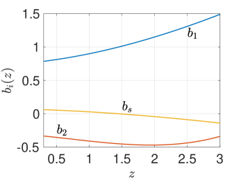
Figure 1: HI bias coefficients (2.5)–(2.7).

Neglecting the lensing term which is subdominant at nearly equal redshifts, the connected 3-point correlation function of the 21cm intensity map at tree level is

$${B}(z_{i},\bm{n}_{i})=\big{\langle}\Delta^{(1)}_{1}\Delta^{(1)}_{2}{\Delta}_{3}^{(2)}\big{\rangle}+\mathrm{2\ perms}.$$ (2.8)

In angular harmonic space,

$${\Delta}(\bm{n},z)=\sum_{\ell m}{\Delta}_{\ell m}(z)Y_{\ell m}(\bm{n}),$$ (2.9)

so that

$${B}(z_{i},\bm{n}_{i})=\sum_{\ell_{i},m_{i}}B^{m_{1}m_{2}m_{3}}_{\ell_{1}\ell_{2}\ell_{3}}(z_{1},z_{2},z_{3})Y_{\ell_{1}m_{1}}(\bm{n}_{1})Y_{\ell_{2}m_{2}}(\bm{n}_{2})Y_{\ell_{3}m_{3}}(\bm{n}_{3}),$$ (2.10)

where

$$B^{m_{1}m_{2}m_{3}}_{\ell_{1}\ell_{2}\ell_{3}}(z_{1},z_{2},z_{3})={\big{\langle}{\Delta}^{(1)}_{\ell_{1}m_{1}}(z_{1})\,{\Delta}^{(1)}_{\ell_{2}m_{2}}(z_{2})\,{\Delta}^{(2)}_{\ell_{3}m_{3}}(z_{3})\big{\rangle}+\mathrm{2\ perms}},$$ (2.11)

is the angular bispectrum.

On account of statistical isotropy, ${B}(z_{i},\bm{n}_{i})$ can only depend on $\bm{n}_{i}\cdot\bm{n}_{j}$. This means that the $m_{i}$ dependence of the bispectrum takes the form

$$B^{m_{1}m_{2}m_{3}}_{\ell_{1}\ell_{2}\ell_{3}}(z_{1},z_{2},z_{3})=\mathcal{G}^{m_{1}m_{2}m_{3}}_{\ell_{1}\ell_{2}\ell_{3}}\,b_{\ell_{1}\ell_{2}\ell_{3}}(z_{1},z_{2},z_{3})\,$$ (2.12)

where $\mathcal{G}^{m_{1}m_{2}m_{3}}_{\ell_{1}\ell_{2}\ell_{3}}$ is the Gaunt integral and $b_{\ell_{1}\ell_{2}\ell_{3}}$ is the reduced angular bispectrum [29]. The reduced bispectrum has contributions from the following six terms [12]:

$$b_{\ell_{1}\ell_{2}\ell_{3}}\left(z_{1},z_{2},z_{3}\right) =b_{\ell_{1}\ell_{2}\ell_{3}}^{\delta^{(2)}}\left(z_{1},z_{2},z_{3}\right)+b_{\ell_{1}\ell_{2}\ell_{3}}^{v^{(2)^{\prime}}}\left(z_{1},z_{2},z_{3}\right)+b_{\ell_{2}^{\prime}\ell_{2}\ell_{3}}^{\delta v^{\prime}}\left(z_{1},z_{2},z_{3}\right)$$

$$+b_{\ell_{1}\ell_{2}\ell_{3}}^{v^{\prime 2}}\left(z_{1},z_{2},z_{3}\right)+b_{\ell_{1}\ell_{2}\ell_{3}}^{\delta^{\prime}v}\left(z_{1},z_{2},z_{3}\right)+b_{\ell_{1}\ell_{2}\ell_{3}}^{v^{\prime\prime}v}\left(z_{1},z_{2},z_{3}\right)$$ (2.13)

The first term arises from the second order density contrast: in Fourier space, it contains monopole, dipole and quadrupole contributions (see [30, 19] for details). The next term is the pure second order RSD contribution and the following four terms arise from the quadratic combinations of first-order velocity and density perturbations appearing in (2.3).

We use the byspectrum code [12] to compute the angular bispectrum in redshift space. The monopole, dipole and quadrupole of the density contribution are shown in contour plots in Figure 2, while Figure 3 displays the different contributions in (2.13). All plots are normalized relative to the angular power spectrum, as in [12], and we assume equal redshifts $z_{i}=1$ and set $\ell_{1}=200$.

Figure 2: Monopole, dipole and quadrupole of the density term in the reduced bispectrum (2.13) of a 21cm intensity map, with $z_{i}=1$ and $\ell_{1}=200$, normalized by angular power spectra as $b_{\ell_{1}\ell_{2}\ell_{3}}/(C_{\ell_{1}}C_{\ell_{2}}+C_{\ell_{1}}C_{\ell_{3}}+C_{\ell_{2}}C_{\ell_{3}})$.

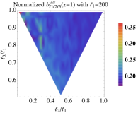
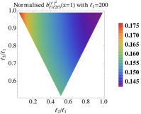
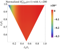
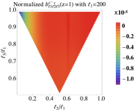
Figure 3: As in Figure 2, for the 6 contributions in (2.13), normalized as above.

The angle-averaged bispectrum is related to the reduced bispectrum as [11]

$$B_{\ell_{1}\ell_{2}\ell_{3}}=\sqrt{\frac{\left(2\ell_{1}+1\right)\left(2\ell_{2}+1\right)\left(2\ell_{3}+1\right)}{4\pi}}\,\left(\begin{array}[]{lll}\ell_{1}&\ell_{2}&\ell_{3}\\ 0&0&0\end{array}\right)\,b_{\ell_{1}\ell_{2}\ell_{3}}\,,$$ (2.14)

where the matrix is the Wigner 3j symbol. In Figure 4, we compare the equilateral ($\ell_{1}=\ell_{2}=\ell_{3}$), ‘squeezed’ ($\ell_{1}=4,\ell_{2}=\ell_{3}$) folded ($\ell_{1}=\ell_{2}=\ell_{3}/2$) and staggered ($\ell_{1}=\ell$, $\ell_{2}=[1.5\ell]$, $\ell_{3}=2\ell$) configurations for the 6 contributions in (2.13) to the angle-averaged bispectrum.

Figure 4 shows that the equilateral shape makes the smallest contribution to the total angle-averaged bispectrum. For all three shapes, the nonlinear RSD terms $B^{\delta^{\prime}v}$ and $B^{v^{\prime\prime}v}$ are negligible. For the other three nonlinear RSD terms, the reduced bispectra $b^{v^{(2)^{\prime}}},b^{\delta v^{\prime}}$ and $b^{v^{\prime 2}}$ are all comparable to the density term $b^{\delta^{(2)}}$. Furthermore, they are all positive. This can be seen since there is no sign change in the plots of Figure 4, while in Figure 3, we see that these terms are all positive for $\ell_{1}=200$. In addition, the four dominant contributions have approximately equal magnitudes for the three shapes. This anticipates what we find below: that including RSD increases the bispectrum by a significant factor.

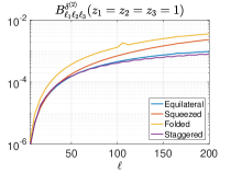
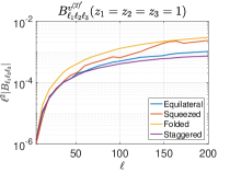
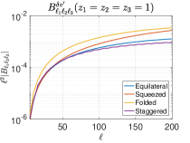
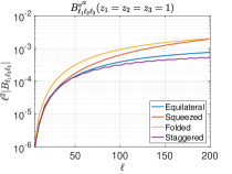
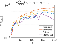
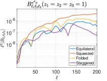
Figure 4: Different contributions in (2.13) to the angle-averaged bispectrum (2.14) of a 21cm intensity map, for 3 configurations (with $\ell_{1}=4$ in the squeezed case) at equal redshifts $z_{i}=1$. In the lower last two panels we used a moving-average filter with window size 2 to smooth numerical features.

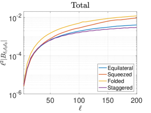
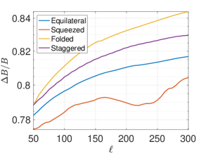
Figure 5: Left: Total angle-averaged bispectrum from Figure 4. Right: RSD fractional contribution (2.15) to this angle-averaged bispectrum.

In order to quantify the RSD contribution to the 21cm intensity bispectrum, we show the total angle-averaged bispectrum in Figure 5 (left panel) and the fractional RSD contribution to the total angle-averaged bispectrum, $\Delta B/B$ in Figure 5 (right panel), where we define

$$\frac{\Delta B}{B}=\frac{B_{\ell_{1}\ell_{2}\ell_{3}}[\mbox{with RSD}]-B_{\ell_{1}\ell_{2}\ell_{3}}[\mbox{no RSD}]}{B_{\ell_{1}\ell_{2}\ell_{3}}[\mbox{with RSD}]}\,.$$ (2.15)

Here ‘no RSD’ denotes the bispectrum with only the $b^{\delta^{(2)}}$ contribution in (2.13) (corresponding to the first 3 terms in (2.3)) and with no RSD in the linear term $\Delta^{(1)}$, i.e., with $\Delta^{(1)}=\delta^{(1)}$.

Interestingly, RSD make up 80% or more of the total signal for all three triangular shapes considered here, so that RSD increases the bispectrum by a factor $\sim$5. Figure 5 corresponds to the maximal RSD contribution, since it is based on zero-width redshift bins. Nevertheless, we expect the RSD contribution to remain dominant for finite but thin redshift bins, similar to the case of the angular power spectrum [6].

3 Detectability of the bispectrum

In order to assess the detectability of the 21cm intensity bispectrum, we consider two next-generation intensity mapping surveys, with SKA-MID [5] and HIRAX [31]. The survey specifications are shown in Table 1. 21cm intensity surveys can be performed in (a) single-dish (SD) mode, where the individual auto-correlations from each dish are simply summed, or in (b) interferometric (IF) mode, where the cross-correlations of all dishes are combined. Surveying in SD mode captures larger scales, while IF mode surveys can resolve smaller scales (see e.g. [4, 32]). SKA-MID is better adapted to SD mode, while HIRAX is designed for IF mode.

Survey	$f_{\mathrm{sky}}$	$N_{\mathrm{d}}$	$t_{\mathrm{tot}}$(hr)	$T_{\mathrm{ins}}$(K)	$D_{\mathrm{d}}$(m)	redshift
SKA	0.48	197	10,000	28	15	0.3–3
HIRAX	0.36	1024	10,000	50	6	0.8–2

Table 1: Specifications that we assume for HIRAX and SKA.

Before we consider the noise and the signal for these 21cm intensity surveys, we need to determine the appropriate limiting angular scales. The $\ell_{i}$ in the bispectrum should each satisfy the condition

$$\ell_{\mathrm{min}}\leq\ell_{i}\leq\ell_{\mathrm{max}}\,,$$ (3.1)

where the lower limit depends on the survey and on foreground cleaning, while the upper limit depends on the survey and the modelling of nonlinearity. Foreground cleaning removes large-scale radial modes in Fourier space, with $k_{\|}\lesssim 0.01h/$Mpc, although this limit can be lowered by the technique of reconstructing large-scale modes using short-scale measurements [33, 34]. In angular harmonic space, modes with $\ell\lesssim 5$ in the power spectrum are effectively lost [35, 6, 36]. We therefore impose

$${\ell_{\mathrm{min}}^{\rm\,fground}\approx 5}\,.$$ (3.2)

The survey sky area $\Omega_{\mathrm{sky}}=4\pi f_{\mathrm{sky}}$ determines the largest possible scale included, which imposes the theoretical lower limit [8]:

$${\ell_{\mathrm{min}}^{\rm\,sky}}=1+{\rm int}\Big{(}\frac{\pi}{\sqrt{\Omega_{\rm sky}}}\,\Big{)}\,,$$ (3.3)

where ‘int’ denotes the integer part. For SKA and HIRAX, this is below 5, and hence (3.2) applies. In fact, IF mode may have $\ell_{\mathrm{min}}$ much larger than 5, since it is the minimum baseline of an interferometer that sets the largest observable mode [36]. Equivalently, there is a maximum scale determined by the field of view in IF pointings [4]. The field of view is determined by the effective beam:

$$\theta_{\mathrm{b}}=1.22\,\frac{\lambda_{21}}{D_{\mathrm{d}}}\,(1+z)\,,$$ (3.4)

where $\lambda_{21}$ is the rest-frame 21cm wavelength and $D_{\rm d}$ is the dish diameter (see Table 1). Then

$${\ell_{\mathrm{min}}^{\rm\,IF}}(z) \approx \frac{2\pi}{\theta_{\mathrm{b}}(z)}$$ (3.5)

$$\approx \frac{147}{1+z}\quad\mbox{for HIRAX}\,.$$ (3.6)

For the angular power spectrum with equal redshift correlations, a theoretical maximum $\ell$ condition is imposed by the range of validity of the tree-level angular power spectrum [6]:

$${\ell_{\rm max}^{\rm\,nl}}(z)=r(z)\,k_{\rm nl}(z)\,,\quad k_{\rm nl}(z)=k_{\rm nl}(0)(1+z)^{2/3}~{}{\rm Mpc}^{-1}\,.$$ (3.7)

For $C_{\ell}$, the nonlinear scale is typically taken as $k_{\rm nl}(0)=0.2h/$ Mpc (see also [37]). In order to reflect the greater sensitivity of the bispectrum to nonlinearity, we follow [25] and assume $k_{\rm nl}(0)=0.1h/$ Mpc, i.e. half of the value for the power spectrum (see also [38]).

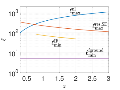
Figure 6: Minimum and maximum scales for SKA (SD) and HIRAX (IF) surveys.

There is also an experimental maximum imposed by the angular resolution of the array: $k_{\perp,{\rm max}}\approx 2\pi D_{\rm res}/(r\lambda)$ where $D_{\rm res}$ is the diameter of the receiving area of the beam array and $\lambda=\lambda_{21}(1+z)$. Thus

$$\ell_{\rm max}^{\rm\,res}(z)\approx{2\pi D_{\rm res}\over\lambda_{21}(1+z)}\,.$$ (3.8)

In SD mode, $D_{\rm res}=D_{\rm d}$ and then,

$$\ell_{\rm max}^{\rm\,res,SD}(z)\approx{2\pi D_{\rm d}\over\lambda_{21}(1+z)}\approx{449\over 1+z}\quad\mbox{for SKA}\,.$$ (3.9)

This can be smaller than (3.7) at high $z$. In IF mode, $D_{\rm res}$ is the maximum baseline, which is $\approx 271\,$m for HIRAX, so that

$$\ell_{\rm max}^{\rm\,res,IF}(z)\approx{2\pi D_{\rm max}\over\lambda_{21}(1+z)}\approx{8108\over 1+z}\quad\mbox{for HIRAX}\,.$$ (3.10)

For all $z$, (3.10) is much larger than (3.7).

In summary, for the surveys considered, we have

SKA (SD): $$\ell_{\rm min}=\ell_{\mathrm{min}}^{\rm\,fground}=5\,,\qquad\qquad~{}\ell_{\mathrm{max}}={\rm min}\big{\{}\ell_{\mathrm{max}}^{\rm\,nl}(z)\,,\,449(1+z)^{-1}\big{\}},~{}~{}~{}~{}$$ (3.11)

HIRAX (IF): $$\ell_{\rm min}=\ell_{\mathrm{min}}^{\rm\,IF}=147(1+z)^{-1}\,,~{}~{}\ell_{\mathrm{max}}=\ell_{\mathrm{max}}^{\rm\,nl}(z)\,.$$ (3.12)

The different limiting scales are shown in Figure 6.

3.1 Intensity mapping noise

To determine the detectability of the angular bispectrum for 21cm intensity surveys with SKA and HIRAX, we have to study the noise for each survey. The 21cm noise power spectrum is dominated by thermal noise (from the sky and the instrument), shot noise can be neglected [6, 39]. For SD and IF modes, the dimensionless noise power spectrum in a single redshift bin has the form [4, 32]

$${\mathcal{N}_{\ell}}(z)=\frac{2\pi f_{\mathrm{sky}}}{t_{\mathrm{tot}}\,\Delta\nu(z)}\left[\frac{T_{\mathrm{sys}}(z)}{\bar{T}_{\mathrm{HI}}(z)}\right]^{2}\,{\alpha_{\ell}(z)\over\beta_{\ell}(z)^{2}}\,.$$ (3.13)

Here $t_{\mathrm{tot}}$ is the observing time (given in Table 1) and $\Delta\nu$ is the bandwidth of the redshift bin with width $\Delta z$:

$$\Delta\nu=\nu_{21}\,\frac{\Delta z}{(1+z)^{2}}\,.$$ (3.14)

The system temperature is made up of instrument and sky contributions:

$$T_{\mathrm{sys}}(z)=T_{\mathrm{ins}}+60\left[\frac{300(1+z)}{\nu_{21}/{\rm MHz}}\right]^{2.55}~{}\mathrm{K}\,,$$ (3.15)

where $T_{\mathrm{ins}}$ is the instrument temperature (see Table 1) and $\nu_{21}=1420\,$MHz. The sky temperature is an approximate fit to observations and other fits can be used. The background 21cm brightness temperature is given by [40]

$$\bar{T}_{\mathrm{HI}}(z)=189h\,\frac{H_{0}(1+z)^{2}}{H(z)}\,\Omega_{\mathrm{HI}}(z)~{}~{}{\rm mK}.$$ (3.16)

Given the paucity of observations, $\Omega_{\rm HI}(z)=\bar{\rho}_{\mathrm{HI}}(z)/\rho_{\rm crit}(0)$ is not well constrained and different simulations can lead to significantly different results. We use the fit [6]

$$\bar{T}_{\mathrm{HI}}(z)=0.056+0.232\,z-0.024\,z^{2}~{}~{}\mathrm{mK}\,.$$ (3.17)

Finally, the dish density factor $\alpha_{\ell}$ and effective beam $\beta_{\ell}$ differ for SD and IF modes as follows [4, 6, 41, 42].

• SD mode:

  $$\alpha^{\rm SD}_{\ell}(z) = {1\over N_{\rm d}}\,,$$ (3.18)

  $$\beta^{\rm SD}_{\ell}(z) = \exp\left[-\frac{\ell(\ell+1)}{16\ln 2}\,\theta_{{\mathrm{b}}}(z)^{2}\right]\,,$$ (3.19)

  where $N_{\rm d}$ is the number of dishes (see Table 1) and $\theta_{\mathrm{b}}$ is given by (3.4).

• IF mode:

  $$\alpha^{\rm IF}_{\ell}(z) = \left[{\lambda(z)^{2}\over A_{\rm eff}}\right]^{2}\,{1\over n_{\rm b}({z},\ell)}\,,$$ (3.20)

  $$\beta^{\rm IF}_{\ell}(z) = {\theta_{\mathrm{b}}(z)},$$ (3.21)

  where $A_{\mathrm{eff}}=0.7\pi D_{\mathrm{d}}^{2}/4$ is the effective dish area and $n_{\rm b}$ is the baseline density in the image plane, determined by the dish distribution. The forms (3.20), (3.21) apply in the case where the pointings (which cover the field of view) are done sequentially.

  HIRAX is an example of a square-packed array. Following [42], we use the fitting formula from [43]:

  $$n_{\rm b}({z},\ell) = {N_{\rm d}}(1+z)^{2}\,\left({\lambda_{21}\over D_{\rm d}}\right)^{2}\left[{a_{1}+a_{2}({L/L_{\rm s}})\over 1+a_{3}({L/L_{\rm s}})^{a_{4}}}\right]\,\exp\left[-\left({L\over L_{\rm s}}\right)^{a_{5}}\right]\,,$$ (3.22)

  $${L(z,\ell)} = {\lambda_{21}\over 2\pi}\,(1+z)\,\ell\,.$$ (3.23)

  Here $L$ is the baseline radial length, ${L_{\rm s}}=D_{\rm d}\sqrt{N_{\rm d}}={192}\,$m is the length of the square side and the fitting parameters are $a_{I}=\big{(}0.4847,-0.3300,1.3156,1.5974,6.8390\big{)}$. See Figure 7.

  

  

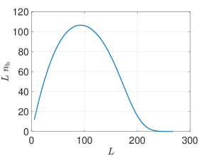
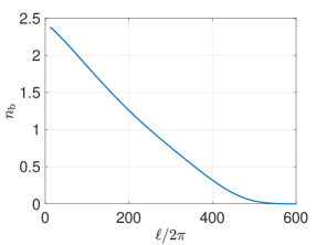
  Figure 7: Baseline density for HIRAX at $z=1$ as a function of $L$ (in m) and $\ell$.

The noise power spectra for SKA and HIRAX surveys are shown at selected redshifts in Figure 8.

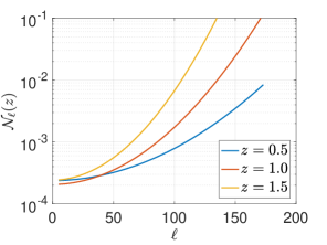
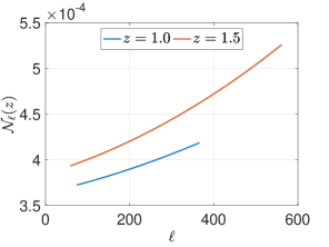
Figure 8: SKA (left) and HIRAX (right) noise at selected redshifts, with $\Delta z=10^{-4}$.

3.2 Signal to noise of the bispectrum

The signal to noise ratio (SNR) for a fixed multipole configuration in a single redshift bin is

$$\mathrm{SNR}_{\ell_{1}\ell_{2}\ell_{3}}(z)=\frac{\big{|}B_{\ell_{1}\ell_{2}\ell_{3}}(z)\big{|}}{\sigma_{B_{\ell_{1}\ell_{2}\ell_{3}}}(z)}\,.$$ (3.24)

The main contribution to the variance, assuming Gaussian initial conditions, comes from the Gaussian part of the 6-point function, given by [12]

$$\sigma^{2}_{B_{\ell_{1}\ell_{2}\ell_{3}}}(z)={f_{\rm sky}^{-1}}\,{{\tilde{C}_{\ell_{1}}(z)\,\tilde{C}_{\ell_{2}}(z)\,\tilde{C}_{\ell_{3}}(z)\,\big{(}1+2\delta_{\ell_{1}\ell_{2}}\delta_{\ell_{2}\ell_{3}}+\delta_{\ell_{1}\ell_{2}}+\delta_{\ell_{2}\ell_{3}}+\delta_{\ell_{3}\ell_{1}}\big{)}}\,,}$$ (3.25)

where

$${\tilde{C}_{\ell}(z)=C_{\ell}(z)+{\cal N}_{\ell}(z)\,,}$$ (3.26)

and the noise is given by (3.13). We have generalised the expression in [12] to include noise and to allow for $f_{\rm sky}\neq 1$.

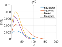
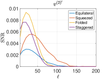
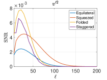
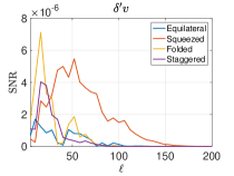
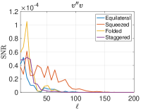
Figure 9: SNR per $\ell$ in one redshift bin for equilateral, squeezed ($\ell_{\rm long}=5$) flattened and staggered shapes for an SKA intensity map (SD mode) at $z=1$, with $\Delta z=10^{-4}$. The panels show the different contributions in (2.13). For the top middle panel we have used the filter of [44], with order 4 and window size 15.

Figure 9 shows the SNR per $\ell$ for the 3 shapes of Figure 4, in the case of SKA in SD mode (see assumption (A3) below for computation details). The different contributions of $B_{\ell_{1}\ell_{2}\ell_{3}}$ to the SNR, for equilateral, squeezed, flattened shapes and staggered configurations, are shown in the 6 panels. As in the case of the theoretical signal, the contribution from the last two panels is subdominant. In all contributions, SNR${}_{\ell_{1}\ell_{2}\ell_{3}}$ becomes negligible for $\ell\gtrsim 150$, owing to the effect of the nonlinear cut-off: at $z=0.5$, (3.7) gives $\ell_{\rm max}^{\rm\,nl}=173$. At higher redshifts, the growing contribution of the beam is what effectively cuts out the higher multipoles. This can be seen in Figure 6, where the beam resolution limit $\ell^{\rm\,res,SD}_{\rm max}$ replaces the nonlinear limit $\ell^{\rm\,nl}_{\rm max}$ as upper limit for $z\gtrsim 0.7$, and in Figure 8 (left), where the noise power spectrum grows much more rapidly with $\ell$ for $z=1$ and 1.5 than for $z=0.5$.

We need to compute the cumulative SNR in a redshift bin, summing over all multipoles and all shapes:

$$\mathrm{SNR}(z)^{2}={\sum_{{\ell_{i}}}\mathrm{SNR}_{\ell_{1}\ell_{2}\ell_{3}}(z)^{2}},$$ (3.27)

where the sum is over all triangular configurations obtained after imposing the Wigner 3j conditions: (a) $\ell_{1}+\ell_{2}+\ell_{3}$ is even, (b) $|\ell_{1}-\ell_{2}|\leq\ell_{3}\leq\ell_{1}+\ell_{2}$. We also use $\ell_{1}\leq\ell_{2}\leq\ell_{3}$, exploiting invariance of the bispectrum under multipole permutations.

In order to demonstrate the detectability of the 21cm bispectrum, we only require a rough estimate of the cumulative SNR. With this in mind, we make three simplifying assumptions to speed up the computations:

1. We neglect the second-order RSD contribution to the signal, including only the linear RSD contribution.

   

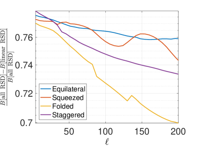
   Figure 10: As in Figure 5, but showing here the fractional contribution (3.28) of linear RSD to the full bispectrum.

   In other words, we use
                             $B[\mbox{linear RSD}]=\big{\langle}\Delta^{(1)}_{1}\Delta^{(1)}_{2}{\big{(}{\Delta}_{3}^{(2)}-R_{3}^{(2)}\big{)}}\big{\rangle}+\mathrm{2\ perms}$,
   where $R^{(2)}$ denotes all the RSD terms in (2.3), instead of
                                 $B[\mbox{all RSD}]=\big{\langle}\Delta^{(1)}_{1}\Delta^{(1)}_{2}{\Delta}_{3}^{(2)}\big{\rangle}+\mathrm{2\ perms}$.
   Figure 10 shows the fractional contribution

   $$B[\mbox{all RSD}]-B[\mbox{linear RSD}]\over B[\mbox{all RSD}]\,$$ (3.28)

   of the the linear RSD to the full bispectrum for the three shapes, similar to Figure 5. From Figure 10, we see that the linear-only RSD signal is $\sim 25\%$ of the full signal. This means that we under-estimate the signal, and therefore the SNR, by a factor of $\sim 4$, when we include only the linear RSD and exclude the nonlinear RSD contribution. We therefore multiply the SNR calculated from $B[\mbox{linear RSD}]$ by a factor of 4, as a rough estimate for the full SNR from $B[\mbox{all RSD}]$. It is interesting to note that while the folded triangles give the largest total signal, the contribution from the non-linear RSD is somewhat smaller for this configuration than for the equilateral, squeezed and staggered ones. It is between 76% and 70% while for the three other configurations it never drops below 73.5%. This is due to the fact that the linear RSD contributes the most to the total signal in the folded configuration (see Fig. 3).

2. The number of possible triangular configurations with non-vanishing Wigner $3j$-symbols rises rapidly as $\ell_{\mathrm{max}}$ increases. We use the simple approximation proposed in [45]:

   $$\mathrm{SNR}_{*}(z)^{2}=n_{\Delta}\,\overline{{\rm SNR}_{\ell_{i}}(z)^{2}}\,,$$ (3.29)

   where $n_{\Delta}$ is the total number of triangles and the arithmetic mean $\overline{{\rm SNR}^{2}_{\ell_{i}}}$ is estimated by computing the SNR for a random selection of triangles.

3. We use a Dirac delta window (see section 3.3) to compute the signal, thus avoiding the numerical complexities of applying a window function in angular redshift space.

   For the smallest possible redshift bin-width for next-generation 21cm intensity maps, we take $\Delta z=10^{-4}$, and we use this in the thermal noise (3.13). Effectively, this assumes that the signal with $\Delta z=0$ is approximately the same as the signal with $\Delta z=10^{-4}$.

The results based on (A1)–(A3) are shown in Tables 2 and 3. As expected, smaller redshifts lead to larger SNR due to larger non-Gaussianities induced by the non-linear gravitational evolution. While the largest SNRs reported here are already promising for single-bin detection, the ${\rm SNR}\lesssim 1$ cases are also relevant in view of tomographic analysis that can potentially benefit from the joint signal of hundreds of bins and their cross-correlations.

Redshift	$\ell_{\mathrm{min}}$	$\ell_{\mathrm{max}}$	$n_{\Delta}$	SNR	SNR
				(linear RSD)	(all RSD, estimated)
0.5	5	173	225598	5.04	$\sim$20
1.0	5	224	485380	0.69	$\sim$3
1.5	5	179	249576	0.09	$\sim$0.4

Table 2: Cumulative SNR in one redshift bin for an SKA survey: using (3.29) for the linear RSD case, and roughly estimating the full linear + nonlinear RSD contribution by applying a factor 4, as described in (A1) above (see Figure 10).

Redshift	$\ell_{\mathrm{min}}$	$\ell_{\mathrm{max}}$	$n_{\Delta}$	SNR	SNR
				(linear RSD)	(all RSD, estimated)
1.0	74	366	1680096	2.78	$\sim$11
1.5	59	561	7021562	1.08	$\sim$4

Table 3: As in Table 2, for a HIRAX survey.

3.3 Consistency checks

In this section, we assess the validity of approximations (A2) and (A3) above. We consider the SKA SD case at $z=0.5$.

For (A2), we estimate the error in SNR induced by approximating the arithmetic mean $\overline{{\rm SNR}_{\ell_{i}}^{2}}$ in (3.29), using only a partial subset of $n_{\rm p}$ multipole triangles, instead of all $n_{\Delta}$ possible triangles. The left panel of Figure 11 shows the deviation with respect to the full result. The latter is obtained by summing over all $n_{\Delta}$ triangles that we compute up to $\ell_{\rm max}=173$. To mitigate the risk of under-estimating the error due to the choice of a particular random draw of $n_{\rm p}$ triangles, we consider 1000 random draws for each $n_{\rm p}$ and compute the maximum cumulative SNR deviation over all draws. From Figure 11, we expect $\lesssim 10\%$ errors when considering $\gtrsim 10^{3}$ triangles.

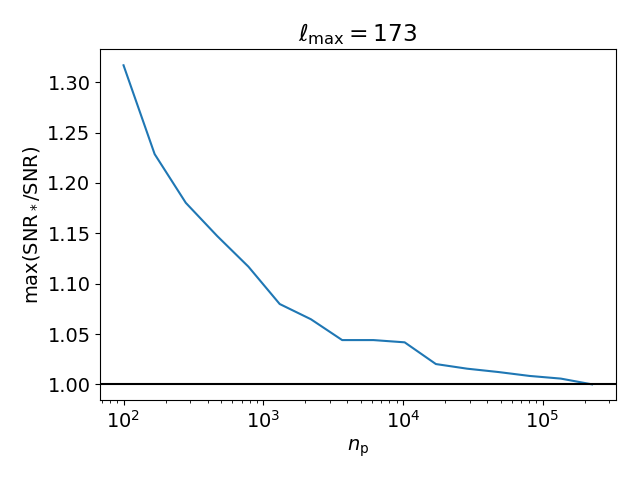
Figure 11: Here we assume an SKA survey at $z=0.5$. Left: Estimated error induced by the approximate cumulative ${{\rm SNR}_{*}}$ in (3.29), obtained by considering only a partial subset of $n_{\rm p}$ multipole triangles. For each $n_{\rm p}$, we consider 1000 random selections of $n_{\rm p}$ multipole triangles and plot the largest deviation with respect to the non-approximate cumulative SNR result (3.27). Right: Approximate cumulative SNR as a function of the maximum multipole $\ell_{\rm max}$ for single redshift bins of different widths.

Next, we check assumption (A3), i.e., whether neglecting the numerically expensive integration over redshift bins recovers the cumulative SNR for the small $\Delta z=10^{-4}$ used in our forecasts. The right panel of Figure 11 shows the approximate cumulative SNR as a function of $\ell_{\rm max}$ for different redshift bin widths. The case labeled $R_{i}(z)=\delta_{D}(z-z_{i})$ corresponds to approximating radial selection functions (see below) as Dirac deltas – i.e., effectively neglecting integration over redshifts, as in our forecasts. For this case, we include a finite $\Delta z=10^{-4}$ in the noise term via (3.14). The other cases consistently integrate over tophat radial selection functions ${R_{i}}(z)$ of width $\Delta z>0$:

$$B_{\ell_{1}\ell_{2}\ell_{3}}^{ijk} = \int{\rm d}z_{1}\,R_{i}(z_{1})\int{\rm d}z_{2}\,R_{j}(z_{2})\int{\rm d}z_{3}\,R_{k}(z_{3})\,B_{\ell_{1}\ell_{2}\ell_{3}}(z_{1},z_{2},z_{3})\,,$$ (3.30)

$$\sigma^{2}_{B_{\ell_{1}\ell_{2}\ell_{3}}^{ijk}} = \int{\rm d}z_{1}\,R_{i}(z_{1})\int{\rm d}z_{2}\,R_{j}(z_{2})\int{\rm d}z_{3}\,R_{k}(z_{3})\,\sigma^{2}_{B_{\ell_{1}\ell_{2}\ell_{3}}}(z_{1},z_{2},z_{3})\,.$$ (3.31)

The variance is given by

$${f_{\rm sky}}\,\sigma^{2}_{B_{\ell_{1}\ell_{2}\ell_{3}}}(z_{1},z_{2},z_{3}) = \tilde{C}_{\ell_{1}}^{11}\tilde{C}_{\ell_{2}}^{22}\tilde{C}_{\ell_{3}}^{33}+\left[\tilde{C}_{\ell_{1}}^{12}\tilde{C}_{\ell_{2}}^{23}\tilde{C}_{\ell_{3}}^{31}+\tilde{C}_{\ell_{1}}^{13}\tilde{C}_{\ell_{2}}^{21}\tilde{C}_{\ell_{3}}^{32}\right]\delta_{\ell_{1}\ell_{2}}\delta_{\ell_{2}\ell_{3}}$$ (3.32)

$${}+\tilde{C}_{\ell_{1}}^{11}\tilde{C}_{\ell_{2}}^{23}\tilde{C}_{\ell_{3}}^{32}\delta_{\ell_{2}\ell_{3}}+\tilde{C}_{\ell_{1}}^{12}\tilde{C}_{\ell_{2}}^{21}\tilde{C}_{\ell_{3}}^{33}\delta_{\ell_{1}\ell_{2}}+\tilde{C}_{\ell_{1}}^{13}\tilde{C}_{\ell_{2}}^{22}\tilde{C}_{\ell_{3}}^{31}\delta_{\ell_{1}\ell_{3}}\,,~{}~{}$$

where $\tilde{C}_{\ell}^{ij}=C_{\ell}(z_{i},z_{j})+{\cal N}_{\ell}(z_{i})\delta_{ij}$. We estimate SNR_∗ by summing over $n_{\rm p}\sim 2000$ triangles for each $\Delta z>0$ case. The left panel of Figure 11 then suggests $\lesssim 10\%$ methodological errors.

Our forecast approximation converges well to the case $\Delta z=10^{-4}$, which validates our analysis. The redshift bin of width $\Delta z=10^{-3}$ leads to a larger signal for the single redshift bin under consideration, given the smaller impact of the noise. However, smoothing the signal over the even larger $\Delta z=10^{-2}$ degrades the SNR as it reduces the signal more strongly than the noise. Note that these individual-bin SNR do not give an accurate picture of the full SNR: smaller $\Delta z$ values allow for a finer tomographic reconstruction, i.e., a larger number of redshift bins – which increases the SNR. We leave the detailed study of an optimal binning strategy as a future development of our work.

4 Conclusions

In this work, we computed the tree-level bispectrum of 21cm intensity mapping induced at second order in perturbations. We worked in directly observable angle-redshift space, which includes all wide-angle, RSD effects. As we discussed equal redshift bins, $z_{1}=z_{2}=z_{3}$, we have neglected lensing which is subdominant in these configurations as shown in [11]. The bispectrum is dominated by the second-order RSD contributions. We expect this finding to be valid also for spectroscopic number count bispectra that also allows bispectrum estimation in relatively small redshift bins.

We computed the SNR for the two near-future surveys SKA-MID (single-dish mode) and HIRAX (interferometric mode). We found that ${\rm SNR}\gtrsim 10$ can be reached in a single bin of width $\Delta z=10^{-4}$ for SKA at redshift $z=0.5$ and for HIRAX at $z=1$. At other redshifts studied in detail, the single-redshift SNR is less than 5 and several bins need to be combined in order to reach an SNR of 10. Another possibility is to increase the bin width. For example, increasing $\Delta z=10^{-4}$ to $\Delta z=10^{-3}$ at $z=0.5$ leads to an increase of the SNR by a factor of $\sim$2. This is, however less than the number of independent bins of width $10^{-4}$ that we could place inside a $\Delta z=10^{-3}$ bin – and the SNR would be further increased by cross correlations. The optimal binning strategy, in both redshift and multipole space, in order to achieve the best SNR, will depend on the detailed observations and is left for a future project. Here we have shown that the detection of the bispectrum with next-generation radio telescopes is feasible. It will also be interesting to investigate whether the SNR of the bispectrum from significantly different redshift bins, where the lensing term is dominant [11], is sufficient to allow its detection. We leave this for a future investigation.

Interesting theoretical questions raised include: How does this ‘guaranteed’ bispectrum, which is a consequence of the nonlinearity of gravity on Gaussian initial perturbations, compare with a possible primordial bispectrum from inflation [46]? How does its shape compare with the simple $f_{\rm NL}$ non-Gaussianity expected in many inflationary models?

Naively, we expect an inflationary $f_{\rm NL}$ to dominate in the squeezed configuration, which is not the case for the bispectrum from nonlinearities investigated here. Therefore, the distinction between these contributions might not be too difficult to detect if the SNR of the experiment and the $f_{\rm NL}$ of the model are sufficiently large.

Another avenue for future investigations is the question of how the additional information in the bispectrum can improve constraints on cosmological model parameters.

References

- [1] J. Fonseca, M. Silva, M. G. Santos and A. Cooray, Cosmology with intensity mapping techniques using atomic and molecular lines, Mon. Not. Roy. Astron. Soc. 464 (2017) 1948 [1607.05288].
- [2] E. D. Kovetz et al., Line-Intensity Mapping: 2017 Status Report, 1709.09066.
- [3] A. Hall, C. Bonvin and A. Challinor, Testing General Relativity with 21-cm intensity mapping, Phys. Rev. D 87 (2013) 064026 [1212.0728].
- [4] P. Bull, P. G. Ferreira, P. Patel and M. G. Santos, Late-time cosmology with 21cm intensity mapping experiments, Astrophys. J. 803 (2015) 21 [1405.1452].
- [5] SKA collaboration, Cosmology with Phase 1 of the Square Kilometre Array: Red Book 2018: Technical specifications and performance forecasts, Publ. Astron. Soc. Austral. 37 (2020) e007 [1811.02743].
- [6] J. Fonseca, J.-A. Viljoen and R. Maartens, Constraints on the growth rate using the observed galaxy power spectrum, JCAP 12 (2019) 028 [1907.02975].
- [7] D. Alonso, P. Bull, P. G. Ferreira, R. Maartens and M. Santos, Ultra large-scale cosmology in next-generation experiments with single tracers, Astrophys. J. 814 (2015) 145 [1505.07596].
- [8] J. Fonseca, S. Camera, M. Santos and R. Maartens, Hunting down horizon-scale effects with multi-wavelength surveys, Astrophys. J. Lett. 812 (2015) L22 [1507.04605].
- [9] O. Umeh, R. Maartens and M. Santos, Nonlinear modulation of the HI power spectrum on ultra-large scales. I, JCAP 03 (2016) 061 [1509.03786].
- [10] M. Jalilvand, E. Majerotto, R. Durrer and M. Kunz, Intensity mapping of the 21 cm emission: lensing, JCAP 01 (2019) 020 [1807.01351].
- [11] E. Di Dio, R. Durrer, G. Marozzi and F. Montanari, The bispectrum of relativistic galaxy number counts, JCAP 01 (2016) 016 [1510.04202].
- [12] E. Di Dio, R. Durrer, R. Maartens, F. Montanari and O. Umeh, The Full-Sky Angular Bispectrum in Redshift Space, JCAP 04 (2019) 053 [1812.09297].
- [13] O. Umeh, S. Jolicoeur, R. Maartens and C. Clarkson, A general relativistic signature in the galaxy bispectrum: the local effects of observing on the lightcone, JCAP 03 (2017) 034 [1610.03351].
- [14] J. Yoo, General Relativistic Description of the Observed Galaxy Power Spectrum: Do We Understand What We Measure?, Phys. Rev. D 82 (2010) 083508 [1009.3021].
- [15] A. Challinor and A. Lewis, The linear power spectrum of observed source number counts, Phys. Rev. D 84 (2011) 043516 [1105.5292].
- [16] C. Bonvin and R. Durrer, What galaxy surveys really measure, Phys. Rev. D 84 (2011) 063505 [1105.5280].
- [17] D. Bertacca, R. Maartens and C. Clarkson, Observed galaxy number counts on the lightcone up to second order: I. Main result, JCAP 09 (2014) 037 [1405.4403].
- [18] J. Yoo and M. Zaldarriaga, Beyond the Linear-Order Relativistic Effect in Galaxy Clustering: Second-Order Gauge-Invariant Formalism, Phys. Rev. D 90 (2014) 023513 [1406.4140].
- [19] E. Di Dio, R. Durrer, G. Marozzi and F. Montanari, Galaxy number counts to second order and their bispectrum, JCAP 12 (2014) 017 [1407.0376].
- [20] A. Kehagias, A. Moradinezhad Dizgah, J. Noreña, H. Perrier and A. Riotto, A Consistency Relation for the Observed Galaxy Bispectrum and the Local non-Gaussianity from Relativistic Corrections, JCAP 08 (2015) 018 [1503.04467].
- [21] S. Jolicoeur, O. Umeh, R. Maartens and C. Clarkson, Imprints of local lightcone projection effects on the galaxy bispectrum. II, JCAP 1709 (2017) 040 [1703.09630].
- [22] S. Jolicoeur, O. Umeh, R. Maartens and C. Clarkson, Imprints of local lightcone projection effects on the galaxy bispectrum. Part III. Relativistic corrections from nonlinear dynamical evolution on large-scales, JCAP 1803 (2018) 036 [1711.01812].
- [23] S. Jolicoeur, A. Allahyari, C. Clarkson, J. Larena, O. Umeh and R. Maartens, Imprints of local lightcone projection effects on the galaxy bispectrum IV: Second-order vector and tensor contributions, JCAP 03 (2019) 004 [1811.05458].
- [24] C. Clarkson, E. M. de Weerd, S. Jolicoeur, R. Maartens and O. Umeh, The dipole of the galaxy bispectrum, Mon. Not. Roy. Astron. Soc. 486 (2019) L101 [1812.09512].
- [25] R. Maartens, S. Jolicoeur, O. Umeh, E. M. De Weerd, C. Clarkson and S. Camera, Detecting the relativistic galaxy bispectrum, JCAP 03 (2020) 065 [1911.02398].
- [26] E. M. de Weerd, C. Clarkson, S. Jolicoeur, R. Maartens and O. Umeh, Multipoles of the relativistic galaxy bispectrum, JCAP 05 (2020) 018 [1912.11016].
- [27] V. Desjacques, D. Jeong and F. Schmidt, Large-Scale Galaxy Bias, Phys. Rept. 733 (2018) 1 [1611.09787].
- [28] J. T. Nielsen and R. Durrer, Higher order relativistic galaxy number counts: dominating terms, JCAP 03 (2017) 010 [1606.02113].
- [29] E. Komatsu and D. N. Spergel, Acoustic signatures in the primary microwave background bispectrum, Phys. Rev. D 63 (2001) 063002 [astro-ph/0005036].
- [30] F. Bernardeau, S. Colombi, E. Gaztanaga and R. Scoccimarro, Large scale structure of the universe and cosmological perturbation theory, Phys. Rept. 367 (2002) 1 [astro-ph/0112551].
- [31] L. Newburgh et al., HIRAX: A Probe of Dark Energy and Radio Transients, Proc. SPIE Int. Soc. Opt. Eng. 9906 (2016) 99065X [1607.02059].
- [32] D. Alonso, P. G. Ferreira, M. J. Jarvis and K. Moodley, Calibrating photometric redshifts with intensity mapping observations, Phys. Rev. D 96 (2017) 043515 [1704.01941].
- [33] H.-M. Zhu, U.-L. Pen, Y. Yu and X. Chen, Recovering lost 21 cm radial modes via cosmic tidal reconstruction, Phys. Rev. D 98 (2018) 043511 [1610.07062].
- [34] C. Modi, M. White, A. Slosar and E. Castorina, Reconstructing large-scale structure with neutral hydrogen surveys, JCAP 11 (2019) 023 [1907.02330].
- [35] A. Witzemann, D. Alonso, J. Fonseca and M. G. Santos, Simulated multitracer analyses with HI intensity mapping, Mon. Not. Roy. Astron. Soc. 485 (2019) 5519 [1808.03093].
- [36] C. J. Schmit, A. F. Heavens and J. R. Pritchard, The gravitational and lensing-ISW bispectrum of 21 cm radiation, Mon. Not. Roy. Astron. Soc. 483 (2019) 4259 [1810.00973].
- [37] E. Di Dio, F. Montanari, R. Durrer and J. Lesgourgues, Cosmological Parameter Estimation with Large Scale Structure Observations, JCAP 01 (2014) 042 [1308.6186].
- [38] V. Yankelevich and C. Porciani, Cosmological information in the redshift-space bispectrum, Mon. Not. Roy. Astron. Soc. 483 (2019) 2078 [1807.07076].
- [39] T.-C. Chang, U.-L. Pen, J. B. Peterson and P. McDonald, Baryon Acoustic Oscillation Intensity Mapping as a Test of Dark Energy, Phys. Rev. Lett. 100 (2008) 091303 [0709.3672].
- [40] F. Villaescusa-Navarro et al., Ingredients for 21 cm Intensity Mapping, Astrophys. J. 866 (2018) 135 [1804.09180].
- [41] M. Jalilvand, E. Majerotto, C. Bonvin, F. Lacasa, M. Kunz, W. Naidoo et al., New Estimator for Gravitational Lensing Using Galaxy and Intensity Mapping Surveys, Phys. Rev. Lett. 124 (2020) 031101 [1907.00071].
- [42] D. Karagiannis, A. z. Slosar and M. Liguori, Forecasts on Primordial non-Gaussianity from 21 cm Intensity Mapping experiments, 1911.03964.
- [43] Cosmic Visions 21 cm collaboration, Inflation and Early Dark Energy with a Stage II Hydrogen Intensity Mapping experiment, 1810.09572.
- [44] A. Savitzky and M. J. E. Golay, Smoothing and differentiation of data by simplified least squares procedures., Analytical Chemistry 36 (1964) 1627.
- [45] F. Montanari and S. Camera, Speeding up the detectability of the harmonic-space galaxy bispectrum, 2008.11131.
- [46] E. Di Dio, H. Perrier, R. Durrer, G. Marozzi, A. Moradinezhad Dizgah, J. Noreña et al., Non-Gaussianities due to Relativistic Corrections to the Observed Galaxy Bispectrum, JCAP 03 (2017) 006 [1611.03720].