exampstyle exampstyle exampstyle exampstyle exampstyle exampstyle exampstyle exampstyle exampstyle exampstyle exampstyle

Shen, Kong

Robust Tensor Principal Component Analysis: Exact Recovery via Deterministic Model

Robust Tensor Principal Component Analysis: Exact Recovery via Deterministic Model

Bo Shen¹, Zhenyu (James) Kong² Department of Industrial and Systems Engineering, Virginia Tech, Blacksburg, VA 24061,
¹boshen@vt.edu, ²zkong@vt.edu Tensor, also known as multi-dimensional array, arises from many applications in signal processing, manufacturing processes, healthcare, among others. As one of the most popular methods in tensor literature, Robust tensor principal component analysis (RTPCA) is a very effective tool to extract the low rank and sparse components in tensors. In this paper, a new method to analyze RTPCA is proposed based on the recently developed tensor-tensor product and tensor singular value decomposition (t-SVD). Specifically, it aims to solve a convex optimization problem whose objective function is a weighted combination of the tensor nuclear norm and the $\ell 1$-norm. In most of literature of RTPCA, the exact recovery is built on the tensor incoherence conditions and the assumption of a uniform model on the sparse support. Unlike this conventional way, in this paper, without any assumption of randomness, the exact recovery can be achieved in a completely deterministic fashion by characterizing the tensor rank-sparsity incoherence, which is an uncertainty principle between the low-rank tensor spaces and the pattern of sparse tensor. Robust tensor principal component analysis, deterministic exact recovery, tensor singular value decomposition, tensor nuclear norm, tensor tubal rank, sparsity.

1 Introduction

Tensor, also known as multidimensional array, recently has attracted much attention in data analytics since real data can be naturally described as a tensor [1]. For example, RGB images are 3-way tensors since they have three channels. As a tensor extension of robust principal component analysis (RPCA) [2],

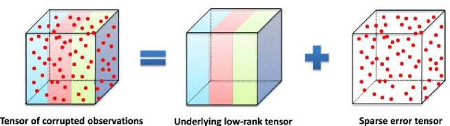
Figure 1: Illustrations of RTPCA [3]

robust tensor principal component analysis (RTPCA) [4, 3] aims to extract the low-rank and sparse tensors from the observed tensor as shown in FIGURE 1, which has been applied to moving object tracking [5], image recovery [6], and background modeling [7]. The tensor extension of RPCA is not easy since the tensor linear algebra is not well defined [8]. One of the major issues is that it is difficult find the tight convex relaxation of the tensor rank. For example, computing the rank of CP decomposition [9] of a tensor is NP-hard [10], leading to an intractable convex relaxation.

Thanks to the development of tensor linear algebra, the extension to RTPCA is possible. Specifically, tensor-tensor product (t-product) [11], which is a generalization of the matrix-matrix product, enjoys many similar properties to the matrix-matrix product. Based on the t-product, any tensors have the tensor singular value decomposition (t-SVD), which further motivates a new tensor rank, namely, tensor tubal rank [12]. Under the framework of tensor linear algebra, the tensor nuclear norm and tensor spectral norm are defined in [4] (see details in Section 2). Based on these definitions, RTPCA [4, 3] is developed, resulting the following problem: given that $\BFcalX=\BFcalL_{0}+\BFcalE_{0}\in\mathbb{R}^{N_{1}\times N_{2}\times N_{3}}$, where $\BFcalL_{0}\in\mathbb{R}^{N_{1}\times N_{2}\times N_{3}}$ is the tensor having low tubal tensor rank and $\BFcalE_{0}\in\mathbb{R}^{N_{1}\times N_{2}\times N_{3}}$ is the sparse tensor, are we able to recover $(\BFcalL_{0},\BFcalE_{0})$ from the following convex optimization problem

$$\begin{aligned} \underset{\BFcalL,\BFcalE}{\text{min}}\quad&\|\BFcalL\|_{*}+\gamma\|\BFcalE\|_{1}\\ \text{subject to}\quad&\BFcalX=\BFcalL+\BFcalE,\end{aligned}$$ (1)

where $\|\BFcalL\|_{*}$ is the tensor nuclear norm (see the definition in Section 2) to enforce the low-rank structure of $\BFcalL$, $\|\BFcalE\|_{1}$ is the $\ell_{1}$ norm to measure the sparsity of $\BFcalE$.

The optimization (1) can be solved by a polynomial-time algorithm, namely, ADMM, with strong recovery guarantees [4]. With the suggested parameter $\gamma=\frac{1}{\sqrt{\max\{N_{1},N_{2}\}N_{3}}}$, the exact recovery is guaranteed with high probability under the assumption of tensor incoherence conditions and a uniform model on the sparse support [4]. Note that this result is the tensor extension of the main results in [2]. Unlike this conventional way, in this paper, the exact recovery is studied in a deterministic model, i.e., without assuming any randomness. Specifically, the contributions of this paper are summarized as follows:

• An uncertainty principle between the low-rank tensor spaces and the sparsity pattern of a tensor is developed, which characterizes fundamental identifiability.

• The deterministic sufficient condition (see Theorem 3) for exact recovery is provided based on the optimization problem (1).

• Classes of low-rank and sparse tensors that satisfy the deterministic sufficient condition in Theorem 3 are identified to guarantee the exact recovery.

1.1 Related Work

Except the RTPCA in (1), there are two other models of TRPCA using t-SVD [6, 13].

Zhang et al. [13] proposes a RTPCA model in order to remove tubal noise, which results the following convex optimization problem

$$\begin{aligned} \underset{\BFcalL,\BFcalE}{\text{min}}\quad&\|\BFcalL\|_{TNN}+\gamma\|\BFcalE\|_{1,1,2}\\ \text{subject to}\quad&\BFcalX=\BFcalL+\BFcalE,\end{aligned}$$ (2)

where $\|\BFcalL\|_{TNN}$ is another definition of tensor nuclear norm (see the definition in Section 2), $\|\BFcalE\|_{1,1,2}$ is defined as the sum of all the $\ell_{2}$ norms of the mode-3 (tube) fibers, i.e., $\sum_{n_{1},n_{2}}\|\BFcalE(n_{1},n_{2},:)\|_{2}$. $\gamma=\frac{1}{\max{(N_{1},N_{2})}}$ is suggested for 3-way tensor $\BFcalX\in\mathbb{R}^{N_{1}\times N_{2}\times N_{3}}$, which is useful in practice. However, there is no exact recovery guarantee in this paper.

Zhou et al. [6] proposes outlier-robust TPCA, which aims to deal with low-rank tensor observations with arbitrary outlier corruption. It has the following convex form:

$$\begin{aligned} \underset{\BFcalL,\BFcalE}{\text{min}}\quad&\|\BFcalL\|_{TNN}+\gamma\|\BFcalE\|_{2,1}\\ \text{subject to}\quad&\BFcalX=\BFcalL+\BFcalE,\end{aligned}$$ (3)

where $\|\BFcalE\|_{2,1}$ is the sum of Frobenius norms of lateral slices, i.e., $\|\BFcalE\|_{2,1}=\sum_{n_{2}=1}^{N_{2}}\|\BFcalE(:,n_{2},:)\|_{F}$. With $\gamma=\frac{1}{\log(N_{2})}$, the exact recovery is guaranteed with high probability under mild conditions. The models in (1), (2) and (3) are all convex optimization models, however, they have different sparse constrains designed for different applications.

1.2 Organizations of the Paper

The remaining of this paper is organized as follows. Section 2 introduces the notations and preliminaries, which are basically related to the tensor algebraic framework in this paper. In Section 3, the deterministic results on RTPCA are presented, which are about the exact recovery under the t-product and t-SVD. The proofs are provided in Section 4 to support the main results. Finally, the implications of this work and future research are discussed in Section 5.

2 Notations and Preliminaries

In this paper, matrices are represented by uppercase boldface letters, namely, $\BFA$; vectors by lowercase boldface letters, namely, $\BFa$; and scalars are denoted by lowercase letters, namely, $a$. The boldface Euler script letters, e.g., $\BFcalA$, denote tensors. $\BFcalA(n_{1},n_{2},n_{3})$ denotes the $(n_{1},n_{2},n_{3})$-th entry of a 3-way tensor $\BFcalA\in\mathbb{R}^{N_{1}\times N_{2}\times N_{3}}$ and $\BFcalA(n_{1},n_{2},:)$ denotes the tube of tensor $\BFcalA\in\mathbb{R}^{N_{1}\times N_{2}\times N_{3}}$. The $n_{1}$-th horizontal, $n_{2}$-th lateral and $n_{3}$-th frontal slices are denoted as $\BFcalA(n_{1},:,:)$, $\BFcalA(:,n_{2},:)$ and $\BFcalA(:,:,n_{3})$, respectively. More often, the frontal slice $\BFcalA(:,:,n_{3})$ is denoted compactly as $\BFA^{(n_{3})}$. The inner product between $\BFcalA$ and $\BFcalB$ in $\mathbb{R}^{N_{1}\times N_{2}\times N_{3}}$ is defined as $\langle\BFcalA,\BFcalB\rangle=\sum_{n_{3}=1}^{N_{3}}\langle\BFA^{(n_{3})},\BFB^{(n_{3})}\rangle$. $\|\BFcalA\|_{F}=\sqrt{\sum_{n_{1},n_{2},n_{3}}|\BFcalA(n_{1},n_{2},n_{3})|^{2}}$, $\|\BFcalA\|_{1}=\sum_{n_{1},n_{2},n_{3}}|\BFcalA(n_{1},n_{2},n_{3})|$ and $\|\BFcalA\|_{\infty}=\max_{n_{1},n_{2},n_{3}}|\BFcalA(n_{1},n_{2},n_{3})|$ are the Frobenius norm, $\ell_{1}$ norm, and infinity norm of $\BFcalA$, respectively.

$\bar{\BFcalA}\in\mathbb{C}^{N_{1}\times N_{2}\times N_{3}}$ denotes the result of Discrete Fourier Transformation (DFT) [14] on $\BFcalA\in\mathbb{R}^{N_{1}\times N_{2}\times N_{3}}$ along the 3-rd dimension, i.e., performing the DFT on all the tubes of $\BFcalA$. $\bar{\BFcalA}$ can be represented using the Matlab command $\normaltt{fft}$ as $\bar{\BFcalA}=\normaltt{fft}(\BFcalA,[\;],3)$. Inversely, $\BFcalA$ can be computed through the inverse FFT, i.e., $\BFcalA=\normaltt{ifft}(\bar{\BFcalA},[\;],3)$. Denote $\bar{\BFA}\in\mathbb{C}^{N_{1}N_{3}\times N_{2}N_{3}}$ as a block diagonal matrix with its $n_{3}$-th block on the diagonal as the $n_{3}$-th frontal slice $\bar{\BFA}^{(n_{3})}$ of $\bar{\BFcalA}$, which has the following form

$$\bar{\BFA}=\normaltt{bdiag}(\bar{\BFcalA})=\begin{bmatrix}\bar{\BFA}^{(1)}&&&\\ &\bar{\BFA}^{(2)}&&\\ &&\ddots&\\ &&&\bar{\BFA}^{(N_{3})}\end{bmatrix},$$

where operator $\normaltt{bdiag}$ maps the tensor $\bar{\BFcalA}$ to the block diagonal matrix $\bar{\BFA}$. Furthermore, the block circulant matrix $\normaltt{bcirc}(\BFcalA)\in\mathbb{R}^{N_{1}N_{3}\times N_{2}N_{3}}$ of $\BFcalA$ is defined as

$$\normaltt{bcirc}(\BFcalA)=\begin{bmatrix}\BFA^{(1)}&\BFA^{(N_{3})}&\cdots&\BFA^{(2)}\\ \BFA^{(2)}&\BFA^{(1)}&\cdots&\BFA^{(3)}\\ \vdots&\vdots&\ddots&\vdots\\ \BFA^{(N_{3})}&\BFA^{(N_{3}-1)}&\cdots&\BFA^{(1)}\end{bmatrix}.$$ (4)

Next, the framework of t-product and t-SVD is introduced. For $\BFcalA\in\mathbb{R}^{N_{1}\times N_{2}\times N_{3}}$, define

$$\normaltt{unfold}(\BFcalA)=\begin{bmatrix}\BFA^{(1)}\\ \BFA^{(2)}\\ \vdots\\ \BFA^{(N_{3})}\end{bmatrix},\;\normaltt{fold}(\normaltt{unfold}(\BFcalA))=\BFcalA,$$

the matricization and tensorization operators [11], respectively.

Definition 1 (T-product [11])

Let $\BFcalA\in\mathbb{R}^{N_{1}\times N_{2}\times N_{3}}$ and $\BFcalB\in\mathbb{R}^{N_{2}\times L\times N_{3}}$. Then the t-product $\BFcalA*\BFcalB$ is defined as,

$$\BFcalA*\BFcalB=\normaltt{fold}(\normaltt{bcirc}(\BFcalA)\cdot\normaltt{unfold}(\BFcalB))\in\mathbb{R}^{N_{1}\times L\times N_{3}}.$$

The t-product can be understood as follows. A 3-way tensor of size $N_{1}\times N_{2}\times N_{3}$ can be regarded as an $N_{1}\times N_{2}$ matrix with each entry being a tube that lies in the third dimension. Thus, the t-product is analogous to the matrix multiplication except that the circular convolution replaces the multiplication operation between the elements.

Definition 2 (Tensor transpose [11])

The tensor transpose of a tensor $\BFcalA\in\mathbb{R}^{N_{1}\times N_{2}\times N_{3}}$ is the tensor $\BFcalA^{\top}\in\mathbb{R}^{N_{1}\times N_{2}\times N_{3}}$ obtained by transposing each of the frontal slices and then reversing the order of transposed frontal slices 2 through $N_{3}$.

As an example, let $\BFcalA\in\mathbb{R}^{N_{1}\times N_{2}\times 4}$, then

$$\BFcalA^{\top}=\normaltt{fold}\left(\begin{bmatrix}\BFA^{(1)\top}\\ \BFA^{(4)\top}\\ \BFA^{(3)\top}\\ \BFA^{(2)\top}\end{bmatrix}\right).$$

Definition 3 (Identity tensor [11])

The identity tensor $\BFcalI\in\mathbb{R}^{N\times N\times N_{3}}$ is the tensor with its first frontal slice being the $N\times N$ identity matrix, and other frontal slices being all zeros.

Definition 4 (Orthogonal tensor [11])

A tensor $\BFcalT\in\mathbb{R}^{N\times N\times N_{3}}$ is orthogonal if it satisfies $\BFcalT^{\top}*\BFcalT=\BFcalT*\BFcalT^{\top}=\BFcalI$.

Definition 5 (F-diagonal Tensor [11])

A tensor is called f-diagonal if each of its frontal slices is a diagonal matrix.

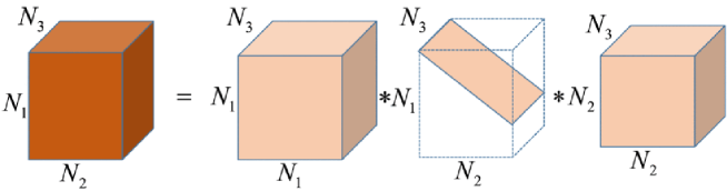
Figure 2: Illustration of t-SVD for an $N_{1}\times N_{2}\times N_{3}$ tensor [15]

Theorem 1 (T-SVD [11])

Let $\BFcalA\in\mathbb{R}^{N_{1}\times N_{2}\times N_{3}}$. Then it can factorized as

$$\BFcalA=\BFcalU*\BFcalS*\BFcalV^{\top},$$ (5)

where $\BFcalU\in\mathbb{R}^{N_{1}\times N_{1}\times N_{3}},\BFcalV\in\mathbb{R}^{N_{2}\times N_{2}\times N_{3}}$ are orthogonal, and $\BFcalS\in\mathbb{R}^{N_{1}\times N_{2}\times N_{3}}$ is an f-diagonal tensor.

The above Theorem 1 shows that any 3-way tensor can be factorized into three components, namely, two orthogonal tensors and an f-diagonal tensor. The FIGURE 2 shows an illustration of the t-SVD factorization. An efficient way for computing t-SVD is implemented in [16].

Definition 6 (Tensor tubal rank [12, 13])

For a tensor $\BFcalA\in\mathbb{R}^{N_{1}\times N_{2}\times N_{3}}$, the tensor tubal rank, denoted as $\normaltt{rank}_{t}(\BFcalA)$, is defined as the number of nonzero singular tubes of $\BFcalS$, where $\BFcalS$ is from the t-SVD of $\BFcalA=\BFcalU*\BFcalS*\BFcalV^{\top}$. Then,

$$\normaltt{rank}_{t}(\BFcalA)=\sharp\{i,\BFcalS(i,i,:)\neq\bm{0}\}.$$

The tensor tubal rank can be further determined by the first slice $\BFcalS(:,:,1)$ of $\BFcalS$ [4], i.e.,

$$\normaltt{rank}_{t}(\BFcalA)=\sharp\{i,\BFcalS(i,i,1)\neq 0\}.$$

The entries on the diagonal of the first frontal slice $\BFcalS(:,:,1)$ of $\BFcalS$ have the same decreasing property as matrix, namely,

$$\BFcalS(1,1,1)\geq\cdots\geq\BFcalS(R,R,1)\geq 0.$$

Hence, the tensor tubal rank is equivalent to the number of nonzero singular values of $\BFcalA$.

Remark 1

It is usually sufficient to compute the reduced version of the t-SVD using the tensor tubal-rank. It’s faster and more economical for storage. In details, suppose $\BFcalA\in\mathbb{R}^{N_{1}\times N_{2}\times N_{3}}$ has tensor tubal-rank $R$, then the skinny t-SVD of $\BFcalA$ is given by

$$\BFcalA=\BFcalU*\BFcalS*\BFcalV^{\top},$$

where $\BFcalU\in\mathbb{R}^{N_{1}\times R\times N_{3}},\BFcalV\in\mathbb{R}^{N_{2}\times R\times N_{3}}$ satisfying $\BFcalU^{\top}\BFcalU=\BFcalI,\BFcalV^{\top}\BFcalV=\BFcalI$, and $\BFcalS\in\mathbb{R}^{R\times R\times N_{3}}$ is an f-diagonal tensor.

The skinny t-SVD will be used throughout the paper unless otherwise noted.

Definition 7 (Tensor spectral norm [4])

The tensor spectral norm of $\BFcalA\in\mathbb{R}^{N_{1}\times N_{2}\times N_{3}}$ is defined as $\|\BFcalA\|\coloneqq\|\normaltt{bcirc}(\BFcalA)\|$.

The tensor nuclear norm, denoted as $\|\BFcalA\|_{*}$, as the dual norm of the tensor spectral norm is defined as follows.

Definition 8 (Tensor nuclear norm [4])

Let $\BFcalA=\BFcalU*\BFcalS*\BFcalV^{\top}$ be t-SVD of $\BFcalA\in\mathbb{R}^{N_{1}\times N_{2}\times N_{3}}$. The tensor nuclear norm of $\BFcalA$ is defined as

$$\|\BFcalA\|_{*}\coloneqq\langle\BFcalS,\BFcalI\rangle=\sum_{i=1}^{R}\BFcalS(i,i,1),$$

where $R=\normaltt{rank}_{t}(\BFcalA)$. Furthermore, the tensor nuclear norm can be rewritten as

$$\|\BFcalA\|_{*}\coloneqq\frac{1}{N_{3}}\|\normaltt{bcirc}(\BFcalA)\|_{*}.$$

Note that there is another tensor nuclear norm, namely, $\|\BFcalA\|_{TNN}$, defined as $\sum_{n_{3}=1}^{N_{3}}\sum_{i=1}^{R}\BFcalS(i,i,n_{3})$ [13, 6]. Based on t-SVD (5), the subgradient of tensor nuclear norm, which is very important to the proofs in Section 4, is defined as follow.

Theorem 2 (Subgradient of tensor nuclear norm)

Let $\BFcalA\in\mathbb{R}^{N_{1}\times N_{2}\times N_{3}}$ with $\normaltt{rank}_{t}(\BFcalA)=R$ and its skinny t-SVD be $\BFcalA=\BFcalU*\BFcalS*\BFcalV^{\top}$. The subdifferential (the set of subgradients) of $\|\BFcalA\|_{*}$ is $\partial\|\BFcalA\|_{*}=\{\BFcalU*\BFcalV^{\top}+\BFcalW|\BFcalU^{\top}*\BFcalW=\bm{0},\BFcalW*\BFcalV=\bm{0},\|\BFcalW\|\leq 1\}$.

Definition 9 (Standard tensor basis [17])

Denote $\mathring{\mathpzc{e}}_{n}$ as the tensor column basis, which is a tensor of $N\times 1\times N_{3}$ with its $(n,1,1)$-th entry equal to $1$ and the rest equal to $0$. Naturally its transpose $\mathring{\mathpzc{e}}_{n}^{\top}$ is called row basis. $\dot{\mathpzc{e}}_{k}$ denotes the tensor tube basis, which is a tensor of size $1\times 1\times N_{3}$ with its $(1,1,k)$-th entry equaling $1$ and the rest equaling $0$.

3 Main Results

Throughout this paper, the analysis focuses on 3-way tensors. The analysis can be extended to $p$-way ($p>3$) tensors using the t-SVD for $p$-way tensors defined in [18]. Given that $\BFcalX=\BFcalL_{0}+\BFcalE_{0}$, where $\BFcalL_{0}$ is an unknown low tubal rank tensor and $\BFcalE_{0}$ is an unknown sparse tensor, the exact recovery $\BFcalL_{0},\BFcalE_{0}$ from $\BFcalX$ without any additional condition is impossible. In the remaining of this section, two natural problems of identifiability are introduced. Based on that, the sufficient condition for the exact recovery is provided. At the end, the classes of low-rank tensor spaces and sparse tensors are identified for the exact recovery.

3.1 Deterministic Exact Recovery

This section is dedicated to presenting the exact recovery results under a deterministic model. We begin with two natural identifiability problems introduced in [19]: (1) the low-rank tensor is very sparse itself; (2) the sparse tensor has all its support concentrated in one horizontal/lateral slice. To deal with these two problems, two concepts are introduced as follows.

(1) The low-rank tensor is very sparse itself. It can be addressed by imposing certain conditions on the tensor spaces $\BFcalU,\BFcalV$ of the low-rank tensor $\BFcalA$. For any tensor $\BFcalA$, the tangent space $T(\BFcalA)$ at $\BFcalA$ with respect to the variety of all tensors with tubal rank less than or equal to $\normaltt{rank}_{t}(\BFcalA)=R$ is the span of tensor spaces $\BFcalU\in\mathbb{R}^{N_{1}\times R\times N_{3}},\BFcalV\in\mathbb{R}^{N_{2}\times R\times N_{3}}$, where $\BFcalA=\BFcalU*\BFcalS*\BFcalV^{\top}$ is the t-SVD. The $T(\BFcalA)$ can be represented as

$$T(\BFcalA)=\{\BFcalU*\BFcalY^{\top}+\BFcalW*\BFcalV^{\top},\BFcalY\in\mathbb{R}^{N_{2}\times R\times N_{3}},\BFcalW\in\mathbb{R}^{N_{1}\times R\times N_{3}}\}.$$ (6)

It always has that $\BFcalA\in T(\BFcalA)$. Next, one of the key definitions, namely, $\xi(\BFcalA)$, in this paper, which measures the “sparsity” of the contraction (tensor nuclear norm less than and equal $1$) in the tangent space as defined in (6), is defined as follows:

$$\xi(\BFcalA)=\underset{\BFcalN\in T(\BFcalA),\|\BFcalN\|\leq 1}{\text{max}}\|\BFcalN\|_{\infty},$$ (7)

where $\|\cdot\|$ and $\|\cdot\|_{\infty}$ are the tensor spectral norm and infinity norm, respectively. If $\xi(\BFcalA)$ is small, it implies that the tensors in the tangent space $T(\BFcalA)$ is not very sparse.

(2) the sparse tensor has all its support concentrated in one horizontal/lateral slice. If the sparse tensor has all its support concentrated in one horizontal/lateral slice; the entries in this horizontal/lateral slice could negate the entries of the corresponding low-rank tensor, thus leaving the tensor tubal rank and the tensor spaces of the low-rank tensor unchanged. In order to address this problem, some conditions should be imposed on the sparsity pattern of the sparse tensor such that the support of tensor is not too concentrated in any horizontal/lateral slice. For any tensor $\BFcalA$, the tangent space $\Omega(\BFcalA)$ with respect to $\normaltt{support}(\BFcalA)$ at $\BFcalA$ is defined as follow:

$$\Omega(\BFcalA)=\{\BFcalN\in\mathbb{R}^{N_{1}\times N_{2}\times N_{3}}|\normaltt{support}(\BFcalN)\subseteq\normaltt{support}(\BFcalA)\}.$$ (8)

Furthermore, $\mu(\BFcalA)$ is defined to measure the “concentration” of the tensor in tangent space $\Omega(\BFcalA)$ (8) as

$$\mu(\BFcalA)=\underset{\BFcalN\in\Omega(\BFcalA),\|\BFcalN\|_{\infty}\leq 1}{\text{max}}\|\BFcalN\|.$$ (9)

If $\mu(\BFcalA)$ is small, it implies that the support for the tensor in the tangent space $\Omega(\BFcalA)$ is not too concentrated in any horizontal/lateral slice.

Before getting into the exact recovery of $(\BFcalL_{0},\BFcalE_{0})$ from the optimization (1), one question deserves further discussion. That is, will $(\BFcalL_{0},\BFcalE_{0})$ be uniquely recovered from its observation $\BFcalX$? Because the convex optimization may have multiple optimal solutions, however, there is only one $(\BFcalL_{0},\BFcalE_{0})$ need to be recovered, which leads to a mismatching situation. In order to avoid this situation, $(\BFcalL_{0},\BFcalE_{0})$ should be the unique minimizer of (1). Here, the necessary and sufficient condition of unique recovery with respect to the tangent spaces $T(\BFcalL_{0})$ and $\Omega(\BFcalE_{0})$ is identified, which can be summarized in the following lemma.

Lemma 1

Assuming that $\BFcalL\in T(\BFcalL_{0})$, $\BFcalE\in\Omega(\BFcalE_{0})$, and $\BFcalL+\BFcalE=\BFcalX$, then $(\BFcalL,\BFcalE)$ has to be $(\BFcalL_{0},\BFcalE_{0})$ if and only if

$$T(\BFcalL_{0})\cap\Omega(\BFcalE_{0})=\{\bm{0}\}.$$ (10)

This lemma tell us that if the $T(\BFcalL_{0})$ and $\Omega(\BFcalE_{0})$ have a trivial intersection, then we will have the unique decomposition. Furthermore, based on the inverse function theorem, the condition in 1 is also a sufficient condition for local identifiability around $(\BFcalL_{0},\BFcalE_{0})$ with respect to the low-rank and sparse tensor varieties. Next, a sufficient condition is provided in terms of numerical values $\xi(\BFcalL_{0})$ and $\mu(\BFcalE_{0})$ to guarantee a trivial intersection between $T(\BFcalL_{0})$ and $\Omega(\BFcalE_{0})$.

Lemma 2

Given any two tensors $\BFcalL_{0}$ and $\BFcalE_{0}$, we have that

$$\xi(\BFcalL_{0})\mu(\BFcalE_{0})<1\Rightarrow T(\BFcalL_{0})\cap\Omega(\BFcalE_{0})=\{\bm{0}\},$$

where $\xi(\BFcalL_{0}),\mu(\BFcalE_{0})$ are defined as (7) and (9), respectively.

This lemma gives a numerical sufficient condition, namely, $\xi(\BFcalL_{0})\mu(\BFcalE_{0})<1$, for an algebraic conclusion, namely, $T(\BFcalL_{0})\cap\Omega(\BFcalE_{0})=\{\bm{0}\}$ in (10). Specifically, both $\xi(\BFcalL_{0})$ and $\mu(\BFcalE_{0})$ being small implies that the tangent spaces $T(\BFcalL_{0})$ and $\Omega(\BFcalE_{0})$ intersect transversally. According to lemma 2, the tensor rank-sparsity uncertainty principle can be obtained easily as a corollary since $\BFcalA\in T(\BFcalA)\cap\Omega(\BFcalA)$. That is, there is no tensor, which can be too sparse while having “diffuse” tensor spaces.

Corollary 1

For any tensor $\BFcalA\neq\bm{0}$, the following holds

$$\xi(\BFcalA)\mu(\BFcalA)\geq 1,$$

where $\xi(\BFcalA),\mu(\BFcalA)$ are defined as (7) and (9), respectively.

In other words, for any tensor $\BFcalA\neq\bm{0}$ both $\xi(\BFcalA)$ and $\mu(\BFcalA)$ cannot be simultaneously small. The key result of this paper is presented in the following theorem.

Theorem 3

Given that $\BFcalX=\BFcalL_{0}+\BFcalE_{0}$ with

$$\xi(\BFcalL_{0})\mu(\BFcalE_{0})<\frac{1}{6},$$

then $(\BFcalL_{0},\BFcalE_{0})$ is the unique minimizer to (1) for the following range of $\gamma$:

$$\gamma\in\left(\frac{\xi(\BFcalL_{0})}{1-4\xi(\BFcalL_{0})\mu(\BFcalE_{0})},\frac{1-3\xi(\BFcalL_{0})\mu(\BFcalE_{0})}{\mu(\BFcalE_{0})}\right).$$

Specifically, $\gamma=\frac{(3\xi(\BFcalL_{0}))^{p}}{(2\mu(\BFcalE_{0}))^{1-p}}$ for any choice of $p\in[0,1]$ is always inside the above range and thus guarantees exact recovery of $(\BFcalL_{0},\BFcalE_{0})$.

The above result shows that if $\xi(\BFcalL_{0})\mu(\BFcalE_{0})<\frac{1}{6}$, the exact recovery of $(\BFcalL_{0},\BFcalE_{0})$ is guaranteed. Note that $\xi(\BFcalL_{0})\mu(\BFcalE_{0})<\frac{1}{6}$ guarantees that the tangent spaces $T(\BFcalL_{0})$ and $\Omega(\BFcalE_{0})$ are sufficiently transverse based on Lemma 2.

3.2 Characterization of Low-Rank and Sparse Tensors

In this section, the classes of low-rank and sparse tensors that satisfy the sufficient condition in Theorem 3. We begin with the low-rank tensor with small $\xi$. Specifically, we show that tensor with tensor spaces that are incoherent with respect to the standard tensor basis have small $\xi$. The tensor incoherence of a tensor subspace $\BFcalS$ can be measured as follows:

$$\beta(\BFcalS)\coloneqq\max_{n}\|\BFcalP_{\BFcalS}\mathring{\mathpzc{e}}_{n}\|_{F},$$ (11)

where $\BFcalP_{\BFcalS}$ is the projection onto the tensor subspace $\BFcalS$. The above definition (11) is the same definition in the Tensor Incoherence Conditions used in [6, 4, 17, 15]. A small value of $\beta(\BFcalS)$ implies that the tensor subspace $\BFcalS$ is not closely aligned with any of the coordinate axes. Given t-SVD $\BFcalL=\BFcalU*\BFcalS*\BFcalV^{\top}$, the incoherence of the tensor spaces of a tensor $\BFcalL\in\mathbb{R}^{N_{1}\times N_{2}\times N_{3}}$ can be defined as

$$\normaltt{inc}(\BFcalL)\coloneqq\max\{\beta(\normaltt{span}(\BFcalU)),\beta(\normaltt{span}(\BFcalV))\},$$ (12)

where $\normaltt{span}(\BFcalU)$ and $\normaltt{span}(\BFcalV)$ are the smallest tensor linear space contains $\BFcalU$ and $\BFcalV$, respectively. One question is that: what is the relationship between $\xi(\BFcalL)$ and $\normaltt{inc}(\BFcalL)$? Because $\xi(\BFcalL)$ is also related to $\normaltt{inc}(\BFcalL)$. The following lemma describes the numerical relationship between $\xi(\BFcalL)$ and $\normaltt{inc}(\BFcalL)$. That is, $\xi(\BFcalL)$ is lower and upper bounded by the tensor incoherence $\normaltt{inc}(\BFcalL)/\sqrt{N_{3}}$ and $\normaltt{inc}(\BFcalL)$, respectively.

Lemma 3

Let $\BFcalL\in\mathbb{R}^{N_{1}\times N_{2}\times N_{3}}$ be any tensor with $\normaltt{inc}(\BFcalL)$ defined in (12). Then the following result holds:

$$\normaltt{inc}(\BFcalL)/\sqrt{N_{3}}\leq\xi(\BFcalL)\leq 2\normaltt{inc}(\BFcalL).$$

Note that the lower bound is different from the result in [19] since we deal with the case of 3-way tensors. If $N_{3}=1$, then Lemma 3 reduces to result in [19].

On the other hand, it is also important to know what kind of sparse tensor has small $\mu$. We find that the $\mu$ of a tensor is upper bounded by the maximum number of nonzero entries per horizontal/lateral slice, lower bounded by the minimum number of nonzero entries per horizontal/lateral slice as stated in the below lemma.

Lemma 4

Let $\BFcalE\in\mathbb{R}^{N_{1}\times N_{2}\times N_{3}}$ be any tensor with at most $\normaltt{deg}_{max}(\BFcalE)$ nonzero entries per horizontal/lateral slice and with at least $\normaltt{deg}_{min}(\BFcalE)$ nonzero entries per horizontal/lateral slice. The following holds

$$\normaltt{deg}_{min}(\BFcalE)\leq\mu(\BFcalE)\leq\normaltt{deg}_{max}(\BFcalE).$$

This lemma provides lower and upper bounds of $\mu$ using $\normaltt{deg}_{min}(\BFcalE)$ and $\normaltt{deg}_{max}(\BFcalE)$, respectively. However, the upper bound can not exactly characterize the sparsity pattern of a tensor, which is essential to determine the value of $\mu$. For example, a 3-way tensor $\BFcalE_{1}\in\mathbb{R}^{N_{1}\times N_{2}\times N_{3}}$ has one tube of 1 and all reaming tubes of 0, then $\normaltt{deg}_{max}(\BFcalE)=N_{3}$, which has the same value of a tensor $\BFcalE_{2}\in\mathbb{R}^{N_{1}\times N_{2}\times N_{3}}$ with 1 everywhere.

Taking advantages of Lemma 3 and 4 together with Theorem 3, the following corollary can be concluded. That is, a small product of the low-rank tensor incoherence and bounded sparse tensor implies the exact recovery from the convex optimization (1).

Corollary 2

Given that $\BFcalX=\BFcalL_{0}+\BFcalE_{0}$ with $\normaltt{inc}(\BFcalL_{0})$ and $\normaltt{deg}_{max}(\BFcalE_{0})$, if we have

$$\normaltt{inc}(\BFcalL_{0})\normaltt{deg}_{max}(\BFcalE_{0})<\frac{1}{12},$$

then $(\BFcalL_{0},\BFcalE_{0})$ is the unique minimizer to (1) for the following range of $\gamma$:

$$\gamma\in\left(\frac{2\normaltt{inc}(\BFcalL_{0})}{1-8\normaltt{inc}(\BFcalL_{0})\normaltt{deg}_{max}(\BFcalE_{0})},\frac{1-\normaltt{inc}(\BFcalL_{0})\normaltt{deg}_{max}(\BFcalE_{0})}{\normaltt{deg}_{max}(\BFcalE_{0})}\right).$$

Specifically, $\gamma=\frac{(6\normaltt{inc}(\BFcalL_{0}))^{p}}{(2\normaltt{deg}_{max}(\BFcalE_{0}))^{1-p}}$ for any choice of $p\in[0,1]$ is always inside the above range and thus guarantees exact recovery of $(\BFcalL_{0},\BFcalE_{0})$.

4 Proofs for Main Results

This section introduces the key steps underlying the proofs related to the main results in Section 3. The notations related to the proofs in this section are introduced first. The orthogonal projection onto the space $T(\BFcalL_{0})$ is denoted as $\BFcalP_{T(\BFcalL_{0})}$. Given t-SVD of $\BFcalL_{0}=\BFcalU*\BFcalS*\BFcalV$, $\BFcalP_{T(\BFcalL_{0})}$ has the following explicit form:

$$\BFcalP_{T(\BFcalL_{0})}(\BFcalA)=\BFcalP_{\BFcalU}*\BFcalA+\BFcalA*\BFcalP_{\BFcalV}-\BFcalP_{\BFcalU}*\BFcalA*\BFcalP_{\BFcalV},$$

where $\BFcalP_{\BFcalU}=\BFcalU*\BFcalU^{\top}$ and $\BFcalP_{\BFcalV}=\BFcalV*\BFcalV^{\top}$. Denote the orthogonal space to $T(\BFcalL_{0})$ as $T(\BFcalL_{0})^{\perp}$. The orthogonal projection onto the space $T(\BFcalL_{0})^{\perp}$ is denoted as $\BFcalP_{T(\BFcalL_{0})^{\perp}}$, which has the following form

$$\BFcalP_{T(\BFcalL_{0})^{\perp}}(\BFcalA)=(\BFcalI_{N_{1}}-\BFcalP_{\BFcalU})*\BFcalA*(\BFcalI_{N_{2}}-\BFcalP_{\BFcalV}),$$

where $\BFcalI_{N_{1}}$ and $\BFcalI_{N_{2}}$ are $N_{1}\times N_{1}\times N_{3}$ and $N_{2}\times N_{2}\times N_{3}$ identity tensors, respectively.

Similarly, the orthogonal projection onto the space $\Omega(\BFcalE_{0})$ is denoted as $\BFcalP_{\Omega(\BFcalE_{0})}$, which simply sets to zero those entries with support not inside $\normaltt{support}(\BFcalE_{0})$. The orthogonal projection onto the space $\Omega(\BFcalE_{0})$ is denoted as $\Omega(\BFcalE_{0})^{\complement}$, which consists of tensors with complementary support, i.e., $\normaltt{support}(\BFcalE_{0})^{\complement}$. The projection onto $\Omega(\BFcalE_{0})^{\complement}$ is denoted as $\BFcalP_{\Omega(\BFcalE_{0})^{\complement}}$.

4.1 Proofs of Lemmas 1 and 2

In this subsection, we provide the proofs related to the tangent spaces $T(\BFcalL)$ and $\Omega(\BFcalE)$. [Proof of Lemma 1] Sufficient condition: It is easily seen by observation.
Necessary condition: This part can be proved by contradiction. Assume that there is a nonzero tensor $\BFcalB$ such that

$$\BFcalB\in T(\BFcalL_{0})\cap\Omega(\BFcalE_{0}).$$

$\BFcalL_{1}=\BFcalL_{0}-\BFcalB$ and $\BFcalE_{1}=\BFcalE_{0}+\BFcalB$ satisfy $\BFcalL_{1}\in T(\BFcalL_{0})$, $\BFcalE_{1}\in\Omega(\BFcalE_{0})$ and $\BFcalL_{1}+\BFcalE_{1}=\BFcalX$, which is a contradiction. [Proof of Lemma 2] First, the following statement is established

$$\underset{\BFcalN\in T(\BFcalL_{0}),\|\BFcalN\|\leq 1}{\text{max}}\|\BFcalP_{\Omega(\BFcalE_{0})}(\BFcalN)\|<1\Rightarrow T(\BFcalL_{0})\cap\Omega(\BFcalE_{0})=\{\bm{0}\}.$$ (13)

The above statement can be proved by contradiction. Assume that the above statement is not true. In other words, there exist $\BFcalN\neq 0$ such that $\BFcalN\in T(\BFcalL_{0})\cap\Omega(\BFcalE_{0})$, $\BFcalN\in T(\BFcalL_{0})$ and $\|\BFcalN\|\leq 1$. $\BFcalN$ can be appropriately scaled such that $\|\BFcalN\|=1$. However, $\|\BFcalP_{\Omega(\BFcalE_{0})}(\BFcalN)\|=\|\BFcalN\|=1$ since $\BFcalN\in T(\BFcalL_{0})\cap\Omega(\BFcalE_{0})$, which leads to a contradiction. Next,

$$\begin{aligned} \underset{\BFcalN\in T(\BFcalL_{0}),\|\BFcalN\|\leq 1}{\text{max}}\|\BFcalP_{\Omega(\BFcalE_{0})}(\BFcalN)\|&\leq\underset{\BFcalN\in T(\BFcalL_{0}),\|\BFcalN\|\leq 1}{\text{max}}\mu(\BFcalE_{0})\|\BFcalP_{\Omega(\BFcalE_{0})}(\BFcalN)\|_{\infty}\\ &\leq\underset{\BFcalN\in T(\BFcalL_{0}),\|\BFcalN\|\leq 1}{\text{max}}\mu(\BFcalE_{0})\|\BFcalN\|_{\infty}\\ &\leq\mu(\BFcalE_{0})\xi(\BFcalL_{0})\\ &<1,\end{aligned}$$ (14)

where the first inequality follows from the definition of $\mu(\BFcalE_{0})$ since $\BFcalP_{\Omega(\BFcalE_{0})}(\BFcalN)\in\Omega(\BFcalE_{0})$, the second inequality is due to the fact that $\|\BFcalP_{\Omega(\BFcalE_{0})}(\BFcalN)\|_{\infty}\leq\|\BFcalN\|_{\infty}$, the third inequality is based on the definition of $\xi(\BFcalE_{0})$, the last inequality is the condition given in Lemma 2. According to (13) and (14), the proof is concluded.

4.2 Proof of Theorem 3

In this subsection, the proof for Theorem 3 is provided, which consists of the following two steps: (1) Sufficient conditions for exact recovery are provided in Lemma 5; (2) The conditions in Theorem 3 satisfy the sufficient conditions given in Lemma 5. We begin with stating the Lemma 5, and then the corresponding proof is provided accordingly.

Lemma 5

Given that $\BFcalX=\BFcalL_{0}+\BFcalE_{0}$. Then $(\BFcalL_{0},\BFcalE_{0})$ is the unique minimizer of (1) if the following conditions are satisfied:

1. $T(\BFcalL_{0})\cap\Omega(\BFcalE_{0})=\{\bm{0}\}$.

2. There exists a dual $\BFcalQ\in\mathbb{R}^{N_{1}\times N_{2}\times N_{3}}$ such that

   1. $\BFcalP_{T(\BFcalL_{0})}(\BFcalQ)=\BFcalU*\BFcalV^{\top}$,

   2. $\|\BFcalP_{T(\BFcalL_{0})^{\perp}}(\BFcalQ)\|<1$,

   3. $\BFcalP_{\Omega(\BFcalE_{0})}(\BFcalQ)=\gamma\normaltt{sign}(\BFcalE_{0})$,

   4. $\|\BFcalP_{\Omega(\BFcalE_{0})^{\complement}}(\BFcalQ)\|_{\infty}<\gamma$,

where $\normaltt{sign}(\BFcalE_{0}(n_{1},n_{2},n_{3}))$ equals $+1$ if $\BFcalE_{0}(n_{1},n_{2},n_{3})>0$, $-1$ if $\BFcalE_{0}(n_{1},n_{2},n_{3})<0$, and $0$ if $\BFcalE_{0}(n_{1},n_{2},n_{3})=0$.

[Proof of Lemma 5] We will show that $(\BFcalL_{0},\BFcalE_{0})$ is the minimizer first. From the optimality conditions for a convex optimization problem [20], $(\BFcalL_{0},\BFcalE_{0})$ is a minimizer if and only if there exists a dual $\BFcalQ\in\mathbb{R}^{N_{1}\times N_{2}\times N_{3}}$ such that

$$\BFcalQ\in\partial\|\BFcalL_{0}\|_{*}\textnormal{ and }\BFcalQ\in\gamma\partial\|\BFcalE_{0}\|_{1}.$$

Here $\BFcalQ\in\partial\|\BFcalL_{0}\|_{*}$ if and only if [21]:

$$\BFcalP_{T(\BFcalL_{0})}(\BFcalQ)=\BFcalU*\BFcalV^{\top}\textnormal{ and }\|\BFcalP_{T(\BFcalL_{0})^{\perp}}(\BFcalQ)\|\leq 1.$$ (15)

Based on the properties of the subdifferential of the $\ell_{1}$ norm, $\BFcalQ\in\gamma\partial\|\BFcalE_{0}\|_{1}$ if and only if

$$\BFcalP_{\Omega(\BFcalE_{0})}(\BFcalQ)=\gamma\normaltt{sign}(\BFcalE_{0})\textnormal{ and }\|\BFcalP_{\Omega(\BFcalE_{0})^{\complement}}(\BFcalQ)\|_{\infty}\leq\gamma.$$ (16)

Therefore, (15) and (16) are necessary and sufficient conditions for $(\BFcalL_{0},\BFcalE_{0})$ to be a minimizer of (1). Hence, $(\BFcalL_{0},\BFcalE_{0})$ is a minimizer of (1) with the conditions given in Lemma 5. Next, we show that $(\BFcalL_{0},\BFcalE_{0})$ is also a unique minimizer. To avoid cluttered notation, in the rest of this subsection, we denote $T=T(\BFcalL_{0})$, $T^{\perp}=T(\BFcalL_{0})^{\perp}$, $\Omega=\Omega(\BFcalE_{0})$, and $\Omega^{\complement}=\Omega(\BFcalE_{0})^{\complement}$.

We consider a feasible perturbation $(\BFcalL_{0}+\BFcalH,\BFcalE_{0}-\BFcalH)$ and show that the objective increases whenever $\BFcalH\neq\bm{0}$, hence proving that $(\BFcalL_{0},\BFcalE_{0})$ is the unique minimizer. To do this, let $(\BFcalQ_{\BFcalL},\BFcalQ_{\BFcalE})$ be an arbitrary subgradient of the objective function in (1) at $(\BFcalL_{0},\BFcalE_{0})$. By the definition of subgradients,

$$\|\BFcalL_{0}+\BFcalH\|_{*}+\gamma\|\BFcalE_{0}-\BFcalH\|_{1}\geq\|\BFcalL_{0}\|_{*}+\gamma\|\BFcalE_{0}\|_{1}+\langle\BFcalQ_{\BFcalL},\BFcalH\rangle-\langle\BFcalQ_{\BFcalE},\BFcalH\rangle$$ (17)

Since $(\BFcalQ_{\BFcalL},\BFcalQ_{\BFcalE})$ is a subgradient of the objective function in (1) at $(\BFcalL_{0},\BFcalE_{0})$, the conditions in (15) and (16) hold, namely,

• $\BFcalQ_{\BFcalL}=\BFcalU*\BFcalV^{\top}+\BFcalP_{T^{\perp}}(\BFcalQ_{\BFcalL})$, with $\|\BFcalP_{T^{\perp}}(\BFcalQ_{\BFcalL})\|\leq 1$.

• $\BFcalQ_{\BFcalE}=\gamma\normaltt{sign}(\BFcalE_{0})+\BFcalP_{\Omega^{\complement}}(\BFcalQ_{\BFcalE})$, with $\|\BFcalP_{\Omega^{\complement}}(\BFcalQ_{\BFcalE})\|_{\infty}\leq\gamma.$

Given the existence of the dual $\BFcalQ$ in Lemma 5, we have that

$$\begin{aligned} \langle\BFcalQ_{\BFcalL},\BFcalH\rangle&=\langle\BFcalU*\BFcalV^{\top}+\BFcalP_{T^{\perp}}(\BFcalQ_{\BFcalL}),\BFcalH\rangle\\ &=\langle\BFcalQ-\BFcalP_{T^{\perp}}(\BFcalQ)+\BFcalP_{T^{\perp}}(\BFcalQ_{\BFcalL}),\BFcalH\rangle\\ &=\langle\BFcalP_{T^{\perp}}(\BFcalQ_{\BFcalL})-\BFcalP_{T^{\perp}}(\BFcalQ),\BFcalH\rangle+\langle\BFcalQ,\BFcalH\rangle\end{aligned}$$ (18)

Similarly, we have that

$$\begin{aligned} \langle\BFcalQ_{\BFcalE},\BFcalH\rangle&=\langle\gamma\normaltt{sign}(\BFcalE_{0})+\BFcalP_{\Omega^{\complement}}(\BFcalQ_{\BFcalE}),\BFcalH\rangle\\ &=\langle\BFcalQ-\BFcalP_{\Omega^{\complement}}(\BFcalQ)+\BFcalP_{\Omega^{\complement}}(\BFcalQ_{\BFcalE}),\BFcalH\rangle\\ &=\langle\BFcalP_{\Omega^{\complement}}(\BFcalQ_{\BFcalE})-\BFcalP_{\Omega^{\complement}}(\BFcalQ),\BFcalH\rangle+\langle\BFcalQ,\BFcalH\rangle\end{aligned}$$ (19)

Putting (18) and (19) together with (17), we have the following inequality

$$\begin{aligned} &\|\BFcalL_{0}+\BFcalH\|_{*}+\gamma\|\BFcalE_{0}-\BFcalH\|_{1}\\ \geq&\|\BFcalL_{0}\|_{*}+\gamma\|\BFcalE_{0}\|_{1}+\langle\BFcalP_{T^{\perp}}(\BFcalQ_{\BFcalL})-\BFcalP_{T^{\perp}}(\BFcalQ),\BFcalH\rangle-\langle\BFcalP_{\Omega^{\complement}}(\BFcalQ_{\BFcalE})-\BFcalP_{\Omega^{\complement}}(\BFcalQ),\BFcalH\rangle\\ =&\|\BFcalL_{0}\|_{*}+\gamma\|\BFcalE_{0}\|_{1}+\langle\BFcalP_{T^{\perp}}(\BFcalQ_{\BFcalL})-\BFcalP_{T^{\perp}}(\BFcalQ),\BFcalP_{T^{\perp}}(\BFcalH)\rangle-\langle\BFcalP_{\Omega^{\complement}}(\BFcalQ_{\BFcalE})-\BFcalP_{\Omega^{\complement}}(\BFcalQ),\BFcalP_{\Omega^{\complement}}(\BFcalH)\rangle.\end{aligned}$$ (20)

Let the t-SVD of $\BFcalP_{T^{\perp}}(\BFcalH)$ as $\tilde{\BFcalU}*\tilde{\BFcalS}*\tilde{\BFcalV}^{\top}$, we set $\BFcalP_{T^{\perp}}(\BFcalQ_{\BFcalL})=\tilde{\BFcalU}*\tilde{\BFcalV}^{\top}$ such that $\|\BFcalP_{T^{\perp}}(\BFcalQ_{\BFcalL})\|=1$ and $\langle\BFcalP_{T^{\perp}}(\BFcalQ_{\BFcalL}),\BFcalP_{T^{\perp}}(\BFcalH)\rangle=\|\BFcalP_{T^{\perp}}(\BFcalH)\|_{*}$, which satisfy the conditions in (15). Furthermore, we set $\BFcalP_{\Omega^{\complement}}(\BFcalQ_{\BFcalE})=-\gamma\normaltt{sign}(\BFcalP_{\Omega^{\complement}}(\BFcalH))$ such that $\|\BFcalP_{\Omega^{\complement}}(\BFcalQ_{\BFcalE})\|_{\infty}=\gamma$ and $\langle\BFcalP_{\Omega^{\complement}}(\BFcalQ_{\BFcalE}),\BFcalP_{\Omega^{\complement}}(\BFcalH)\rangle=-\gamma\|\BFcalP_{\Omega^{\complement}}(\BFcalH)\|_{1}$, which satisfy the conditions in (16). Based on the carefully selected $\BFcalP_{T^{\perp}}(\BFcalQ_{\BFcalL})$ and $\BFcalP_{\Omega^{\complement}}(\BFcalQ_{\BFcalE})$, the inequality (20) can be simplified as

$$\begin{aligned} &\|\BFcalL_{0}+\BFcalH\|_{*}+\gamma\|\BFcalE_{0}-\BFcalH\|_{1}\\ \geq&\|\BFcalL_{0}\|_{*}+\gamma\|\BFcalE_{0}\|_{1}+\langle\BFcalP_{T^{\perp}}(\BFcalQ_{\BFcalL})-\BFcalP_{T^{\perp}}(\BFcalQ),\BFcalP_{T^{\perp}}(\BFcalH)\rangle-\langle\BFcalP_{\Omega^{\complement}}(\BFcalQ_{\BFcalE})-\BFcalP_{\Omega^{\complement}}(\BFcalQ),\BFcalP_{\Omega^{\complement}}(\BFcalH)\rangle\\ =&\|\BFcalL_{0}\|_{*}+\gamma\|\BFcalE_{0}\|_{1}+\|\BFcalP_{T^{\perp}}(\BFcalH)\|_{*}-\langle\BFcalP_{T^{\perp}}(\BFcalQ),\BFcalP_{T^{\perp}}(\BFcalH)\rangle+\gamma\|\BFcalP_{\Omega^{\complement}}(\BFcalH)\|_{1}+\langle\BFcalP_{\Omega^{\complement}}(\BFcalQ),\BFcalP_{\Omega^{\complement}}(\BFcalH)\rangle\\ \geq&\|\BFcalL_{0}\|_{*}+\gamma\|\BFcalE_{0}\|_{1}+(1-\|\BFcalP_{T^{\perp}}(\BFcalQ)\|)\|\BFcalP_{T^{\perp}}(\BFcalH)\|_{*}+(\gamma-\|\BFcalP_{\Omega^{\complement}}(\BFcalQ)\|_{\infty})\|\BFcalP_{\Omega^{\complement}}(\BFcalH)\|_{1}\\ >&\|\BFcalL_{0}\|_{*}+\gamma\|\BFcalE_{0}\|_{1},\end{aligned}$$ (21)

where the first inequality is based on carefully selected $\BFcalP_{T^{\perp}}(\BFcalQ_{\BFcalL})$ and $\BFcalP_{\Omega^{\complement}}(\BFcalQ_{\BFcalE})$, the second inequality is due to the fact that $|\langle\BFcalP_{T^{\perp}}(\BFcalQ),\BFcalP_{T^{\perp}}(\BFcalH)\rangle|\leq\|\BFcalP_{T^{\perp}}(\BFcalQ)\|\cdot\|\BFcalP_{T^{\perp}}(\BFcalH)\|_{*}$ and $|\langle\BFcalP_{\Omega^{\complement}}(\BFcalQ),\BFcalP_{\Omega^{\complement}}(\BFcalH)\rangle|\leq\|\BFcalP_{\Omega^{\complement}}(\BFcalQ)\|_{\infty}\cdot\|\BFcalP_{\Omega^{\complement}}(\BFcalH)\|_{1}$, and the last inequality is due to the given conditions in Lemma 5, namely, $\|\BFcalP_{T(\BFcalL_{0})^{\perp}}(\BFcalQ)\|<1$ and $\|\BFcalP_{\Omega(\BFcalE_{0})^{\complement}}(\BFcalQ)\|_{\infty}<\gamma$, and $\|\BFcalP_{T^{\perp}}(\BFcalH)\|_{*}+\|\BFcalP_{\Omega^{\complement}}(\BFcalH)\|_{1}>0$, which is derived from $\BFcalH\neq\bm{0}$ and the given condition $T(\BFcalL_{0})\cap\Omega(\BFcalE_{0})=\{\bm{0}\}$.

The above inequality (21) leads to the statement that $\|\BFcalL_{0}+\BFcalH\|_{*}+\gamma\|\BFcalE_{0}-\BFcalH\|_{1}>\|\BFcalL_{0}\|_{*}+\gamma\|\BFcalE_{0}\|_{1}$ unless $\BFcalH=\bm{0}$. Thus, the uniqueness of $(\BFcalL_{0},\BFcalE_{0})$ is proved here.

[Proof of Theorem 3] The proof of Theorem 3 can be viewed as a dual certification. That is, given the condition in Theorem 3, there exist a dual $\BFcalQ$ satisfying the sufficient conditions provided in Lemma 5. We aims to construct a dual $\BFcalQ$ by considering candidates in the direct sum $T\bigoplus\Omega$ of the tangent spaces. Since $\xi(\BFcalL_{0})\mu(\BFcalE_{0})<\frac{1}{6}$, we can conclude from Lemma 2 that there exist a unique $\hat{\BFcalQ}$ such that $\BFcalP_{T}(\hat{\BFcalQ})=\BFcalU*\BFcalV^{\top}$ and $\BFcalP_{\Omega}(\hat{\BFcalQ})=\gamma\normaltt{sign}(\BFcalE_{0})$. The rest of this proof shows that if $\xi(\BFcalL_{0})\mu(\BFcalE_{0})<\frac{1}{6}$, then the projections of such a $\hat{\BFcalQ}$ onto $T^{\perp}$ and onto $\Omega^{\complement}$ will be small, namely, $\|\BFcalP_{T(\BFcalL_{0})^{\perp}}(\BFcalQ)\|<1$ and $\|\BFcalP_{\Omega(\BFcalE_{0})^{\complement}}(\BFcalQ)\|_{\infty}<\gamma$.

Note that $\hat{\BFcalQ}$ can be uniquely decomposed into two parts, namely, an element of $T$ and an element of $\Omega$, which can be expressed as $\hat{\BFcalQ}=\BFcalQ_{T}+\BFcalQ_{\Omega}$ where $\BFcalQ_{T}\in T$ and $\BFcalQ_{\Omega}\in\Omega$. Let $\BFcalQ_{T}=\BFcalU*\BFcalV^{\top}+\BFcalH_{T}$ and $\BFcalQ_{\Omega}=\gamma\normaltt{sign}(\BFcalE_{0})+\BFcalH_{\Omega}$. Accordingly,

$$\BFcalP_{T}(\hat{\BFcalQ})=\BFcalU*\BFcalV^{\top}+\BFcalH_{T}+\BFcalP_{T}(\gamma\normaltt{sign}(\BFcalE_{0})+\BFcalH_{\Omega}).$$

Since $\BFcalP_{T}(\hat{\BFcalQ})=\BFcalU*\BFcalV^{\top}$, the below can be obtained

$$\BFcalH_{T}=-\BFcalP_{T}(\gamma\normaltt{sign}(\BFcalE_{0})+\BFcalH_{\Omega}).$$

Similarly,

$$\BFcalH_{\Omega}=-\BFcalP_{\Omega}(\BFcalU*\BFcalV^{\top}+\BFcalH_{T}).$$

Next,

$$\begin{aligned} \|\BFcalP_{T^{\perp}}(\hat{\BFcalQ})\|&=\|\BFcalP_{T^{\perp}}(\gamma\normaltt{sign}(\BFcalE_{0})+\BFcalH_{\Omega})\|\\ &\leq\|\gamma\normaltt{sign}(\BFcalE_{0})+\BFcalH_{\Omega}\|\\ &\leq\mu(\BFcalE_{0})\|\gamma\normaltt{sign}(\BFcalE_{0})+\BFcalH_{\Omega}\|_{\infty}\\ &\leq\mu(\BFcalE_{0})(\gamma+\|\BFcalH_{\Omega}\|_{\infty}),\end{aligned}$$ (22)

where the first inequality is obvious, the second inequality is based on the definition of $\mu(\BFcalE_{0})$ since $\gamma\normaltt{sign}(\BFcalE_{0})+\BFcalH_{\Omega}\in\Omega$. The bound $\|\BFcalP_{\Omega^{\complement}}(\hat{\BFcalQ})\|_{\infty}$ can be obtained as follows

$$\begin{aligned} \|\BFcalP_{\Omega^{\complement}}(\hat{\BFcalQ})\|_{\infty}&=\|\BFcalP_{\Omega^{\complement}}(\BFcalU*\BFcalV^{\top}+\BFcalH_{T})\|_{\infty}\\ &\leq\|\BFcalU*\BFcalV^{\top}+\BFcalH_{T}\|_{\infty}\\ &\leq\xi(\BFcalL_{0})\|\BFcalU*\BFcalV^{\top}+\BFcalH_{T}\|\\ &\leq\xi(\BFcalL_{0})(1+\|\BFcalH_{T}\|),\end{aligned}$$ (23)

where the first inequality is obvious, the second inequality is based on the definition of $\xi(\BFcalL_{0})$ since $\BFcalU*\BFcalV^{\top}+\BFcalH_{T}\in T$, and the last inequality is due to the triangle inequality for tensor spectral norm. Furthermore, the bounds for $\|\BFcalH_{T}\|$ and $\|\BFcalH_{\Omega}\|_{\infty}$ are derived, respectively.

$$\begin{aligned} \|\BFcalH_{T}\|&=\|\BFcalP_{T}(\gamma\normaltt{sign}(\BFcalE_{0})+\BFcalH_{\Omega})\|\\ &\leq 2\|\gamma\normaltt{sign}(\BFcalE_{0})+\BFcalH_{\Omega}\|\\ &\leq 2\mu(\BFcalE_{0})\|\gamma\normaltt{sign}(\BFcalE_{0})+\BFcalH_{\Omega}\|_{\infty}\\ &\leq 2\mu(\BFcalE_{0})(\gamma+\|\BFcalH_{\Omega}\|_{\infty}),\end{aligned}$$ (24)

where the first inequality is due to the fact that $\|\BFcalP_{T}(\BFcalA)\|\leq 2\|\BFcalA\|$, the second inequality is based on the definition $\mu(\BFcalE_{0})$, and the last inequality is obtained by the triangle inequality for $\|\cdot\|_{\infty}$. Similarly,

$$\begin{aligned} \|\BFcalH_{\Omega}\|_{\infty}&=\|\BFcalP_{\Omega}(\BFcalU*\BFcalV^{\top}+\BFcalH_{T})\|_{\infty}\\ &\leq\|\BFcalU*\BFcalV^{\top}+\BFcalH_{T}\|_{\infty}\\ &\leq\xi(\BFcalL_{0})\|\BFcalU*\BFcalV^{\top}+\BFcalH_{T}\|\\ &\leq\xi(\BFcalL_{0})(1+\|\BFcalH_{T}\|),\end{aligned}$$ (25)

where the first inequality is obvious, the second inequality is based on the definition $\xi(\BFcalL_{0})$, and the last inequality is obtained by the triangle inequality for tensor spectral norm $\|\cdot\|$.

Plugging (25) into (24), we have that

$$\begin{aligned} &\|\BFcalH_{T}\|\leq 2\mu(\BFcalE_{0})(\gamma+\xi(\BFcalL_{0})(1+\|\BFcalH_{T}\|))\\ \Rightarrow&\|\BFcalH_{T}\|\leq\frac{2\gamma\mu(\BFcalE_{0})+2\xi(\BFcalL_{0})\mu(\BFcalE_{0})}{1-2\xi(\BFcalL_{0})\mu(\BFcalE_{0})}.\end{aligned}$$ (26)

Inversely, plugging (24) into (25),

$$\begin{aligned} &\|\BFcalH_{\Omega}\|_{\infty}\leq\xi(\BFcalL_{0})(1+2\mu(\BFcalE_{0})(\gamma+\|\BFcalH_{\Omega}\|_{\infty}))\\ \Rightarrow&\|\BFcalH_{\Omega}\|_{\infty}\leq\frac{\xi(\BFcalL_{0})+2\gamma\xi(\BFcalL_{0})\mu(\BFcalE_{0})}{1-2\xi(\BFcalL_{0})\mu(\BFcalE_{0})}.\end{aligned}$$ (27)

Now we can bound $\|\BFcalP_{T^{\perp}}(\hat{\BFcalQ})\|$ by combining (22) and (27),

$$\begin{aligned} \|\BFcalP_{T^{\perp}}(\hat{\BFcalQ})\|&\leq\mu(\BFcalE_{0})(\gamma+\frac{\xi(\BFcalL_{0})+2\gamma\xi(\BFcalL_{0})\mu(\BFcalE_{0})}{1-2\xi(\BFcalL_{0})\mu(\BFcalE_{0})})\\ &=\mu(\BFcalE_{0})\frac{\gamma+\xi(\BFcalL_{0})}{1-2\xi(\BFcalL_{0})\mu(\BFcalE_{0})}\\ &<\mu(\BFcalE_{0})\frac{\frac{1-3\xi(\BFcalL_{0})\mu(\BFcalE_{0})}{\mu(\BFcalE_{0})}+\xi(\BFcalL_{0})}{1-2\xi(\BFcalL_{0})\mu(\BFcalE_{0})}\\ &=1,\end{aligned}$$

where the first inequality is given by plugging (27) into (22), the second inequality is due to the assumption in Theorem 3, namely, $\gamma<\frac{1-3\xi(\BFcalL_{0})\mu(\BFcalE_{0})}{\mu(\BFcalE_{0})}$.

In the end of this proof, the bound for $\|\BFcalP_{\Omega^{\complement}}(\hat{\BFcalQ})\|_{\infty}$ can be obtained by combining by plugging (26) into (23),

$$\begin{aligned} \|\BFcalP_{\Omega^{\complement}}(\hat{\BFcalQ})\|_{\infty}&\leq\xi(\BFcalL_{0})(1+\frac{2\gamma\mu(\BFcalE_{0})+2\xi(\BFcalL_{0})\mu(\BFcalE_{0})}{1-2\xi(\BFcalL_{0})\mu(\BFcalE_{0})})\\ &=\xi(\BFcalL_{0})\frac{1+2\gamma\mu(\BFcalE_{0})}{1-2\xi(\BFcalL_{0})\mu(\BFcalE_{0})}\\ &=\left[\xi(\BFcalL_{0})\frac{1+2\gamma\mu(\BFcalE_{0})}{1-2\xi(\BFcalL_{0})\mu(\BFcalE_{0})}-\gamma\right]+\gamma\\ &=\left[\frac{\xi(\BFcalL_{0})-\gamma(1-4\xi(\BFcalL_{0})\mu(\BFcalE_{0}))}{1-2\xi(\BFcalL_{0})\mu(\BFcalE_{0})}\right]+\gamma\\ &<\left[\frac{\xi(\BFcalL_{0})-\xi(\BFcalL_{0})}{1-2\xi(\BFcalL_{0})\mu(\BFcalE_{0})}\right]+\gamma\\ &=\gamma,\end{aligned}$$

where the last inequality is due to the assumption in Theorem 3, that is, $\gamma>\frac{\xi(\BFcalL_{0})}{1-4\xi(\BFcalL_{0})\mu(\BFcalE_{0})}$. Hence, the dual certification is done.

In addition, we can verify the lower and upper bounds for $\gamma$ is feasible through the following claim

$$\xi(\BFcalL_{0})\mu(\BFcalE_{0})<\frac{1}{6}\Rightarrow\frac{\xi(\BFcalL_{0})}{1-4\xi(\BFcalL_{0})\mu(\BFcalE_{0})}<\frac{1-3\xi(\BFcalL_{0})\mu(\BFcalE_{0})}{\mu(\BFcalE_{0})},$$ (28)

which can be obtained by computing the roots for a quadratic function. For any $p\in[0,1]$, we can verify that $\gamma=\frac{(3\xi(\BFcalL_{0}))^{p}}{(2\mu(\BFcalE_{0}))^{1-p}}$ is always inside the above range.

4.3 Proofs of Lemmas 3 and 4

In this subsection, the proofs for the bounds for $\xi(\BFcalL)$ and $\mu(\BFcalE)$ by characterizing $\normaltt{inc}(\BFcalL)$ and $\normaltt{deg}_{min}(\BFcalE),\normaltt{deg}_{max}(\BFcalE)$ are provided. [Proof of Lemma 3] Given t-SVD $\BFcalL=\BFcalU*\BFcalS*\BFcalV$,

$$\begin{aligned} \xi(\BFcalL)&=\underset{\BFcalN\in T(\BFcalL),\|\BFcalN\|\leq 1}{\text{max}}\|\BFcalN\|_{\infty}\\ &=\underset{\BFcalN\in T(\BFcalL),\|\BFcalN\|\leq 1}{\text{max}}\|\BFcalP_{T(\BFcalL)}(\BFcalN)\|_{\infty}\\ &\leq\underset{\|\BFcalN\|\leq 1}{\text{max}}\|\BFcalP_{T(\BFcalL)}(\BFcalN)\|_{\infty}\\ &\leq\underset{\BFcalN\textnormal{orthogonal}}{\text{max}}\|\BFcalP_{T(\BFcalL)}(\BFcalN)\|_{\infty}\\ &\leq\underset{\BFcalN\textnormal{orthogonal}}{\text{max}}\|\BFcalP_{\BFcalU}*\BFcalN\|_{\infty}+\underset{\BFcalN\textnormal{orthogonal}}{\text{max}}\|(\BFcalI_{N_{1}}-\BFcalP_{\BFcalU})*\BFcalN*\BFcalP_{\BFcalV}\|_{\infty},\end{aligned}$$ (29)

where the second inequality is due to the fact that the maximum of a convex function over a convex set is achieved at one of the extreme points of the constraint set. The orthogonal tensors are the extreme points of the set of contractions. The last inequality is the triangle inequality. We further show the upper bounds for the two terms in the last line of (29), namely, $\underset{\BFcalN\textnormal{orthogonal}}{\text{max}}\|\BFcalP_{\BFcalU}*\BFcalN\|_{\infty}$ and $\underset{\BFcalN\textnormal{orthogonal}}{\text{max}}\|(\BFcalI_{N_{1}}-\BFcalP_{\BFcalU})*\BFcalN*\BFcalP_{\BFcalV}\|_{\infty}$.

$$\begin{aligned} \underset{\BFcalN\textnormal{orthogonal}}{\text{max}}\|\BFcalP_{\BFcalU}*\BFcalN\|_{\infty}&=\underset{\BFcalN\textnormal{orthogonal}}{\text{max}}\;\underset{n_{1},n_{2},n_{3}}{\text{max}}|\mathring{\mathpzc{e}}_{n_{1}}^{\top}*\BFcalP_{\BFcalU}*\BFcalN*\mathring{\mathpzc{e}}_{n_{2}}(1,1,n_{3})|\\ &\leq\underset{\BFcalN\textnormal{orthogonal}}{\text{max}}\;\underset{n_{1},n_{2}}{\text{max}}\|\mathring{\mathpzc{e}}_{n_{1}}^{\top}*\BFcalP_{\BFcalU}\|_{F}\|\BFcalN*\mathring{\mathpzc{e}}_{n_{2}}\|_{F}\\ &=\underset{n_{1}}{\text{max}}\|\BFcalP_{\BFcalU}*\mathring{\mathpzc{e}}_{n_{1}}\|_{F}\times\underset{\BFcalN\textnormal{orthogonal}}{\text{max}}\;\underset{n_{2}}{\text{max}}\|\BFcalN*\mathring{\mathpzc{e}}_{n_{2}}\|_{F}\\ &=\beta(\BFcalU),\end{aligned}$$ (30)

where the first inequality is based on the property of t-SVD and the famous Cauchy–Schwarz inequality (Note that $\mathring{\mathpzc{e}}_{n_{1}}^{\top}*\BFcalP_{\BFcalU}*\BFcalN*\mathring{\mathpzc{e}}_{n_{2}}$ is a tensor with size $1\times 1\times N_{3}$).

$$\begin{aligned} &\underset{\BFcalN\textnormal{orthogonal}}{\text{max}}\|(\BFcalI_{N_{1}}-\BFcalP_{\BFcalU})*\BFcalN*\BFcalP_{\BFcalV}\|_{\infty}\\ =&\underset{\BFcalN\textnormal{orthogonal}}{\text{max}}\;\underset{n_{1},n_{2},n_{3}}{\text{max}}|\mathring{\mathpzc{e}}_{n_{1}}^{\top}*(\BFcalI_{N_{1}}-\BFcalP_{\BFcalU})*\BFcalN*\BFcalP_{\BFcalV}*\mathring{\mathpzc{e}}_{n_{2}}(1,1,n_{3})|\\ \leq&\underset{\BFcalN\textnormal{orthogonal}}{\text{max}}\;\underset{n_{1},n_{2}}{\text{max}}\|\mathring{\mathpzc{e}}_{n_{1}}^{\top}*(\BFcalI_{N_{1}}-\BFcalP_{\BFcalU})\|_{F}\|\BFcalN*\BFcalP_{\BFcalV}*\mathring{\mathpzc{e}}_{n_{2}}\|_{F}\\ =&\underset{n_{1}}{\text{max}}\|\mathring{\mathpzc{e}}_{n_{1}}^{\top}*(\BFcalI_{N_{1}}-\BFcalP_{\BFcalU})\|_{F}\times\underset{\BFcalN\textnormal{orthogonal}}{\text{max}}\;\underset{n_{2}}{\text{max}}\|\BFcalN*\BFcalP_{\BFcalV}*\mathring{\mathpzc{e}}_{n_{2}}\|_{F}\\ \leq&1\times\underset{n_{2}}{\text{max}}\|\BFcalP_{\BFcalV}*\mathring{\mathpzc{e}}_{n_{2}}\|_{F}\\ =&\beta(\BFcalV),\end{aligned}$$ (31)

where the first inequality is based on the property of t-SVD and the famous Cauchy–Schwarz inequality (Note that $\mathring{\mathpzc{e}}_{n_{1}}^{\top}*(\BFcalI_{N_{1}}-\BFcalP_{\BFcalU})*\BFcalN*\BFcalP_{\BFcalV}*\mathring{\mathpzc{e}}_{n_{2}}$ is a tensor with size $1\times 1\times N_{3}$). Then, plugging (30) and (31) into (29),

$$\xi(\BFcalL)\leq\beta(\BFcalU)+\beta(\BFcalV)\leq 2\normaltt{inc}(\BFcalL).$$ (32)

Hence the upper bound on $\xi(\BFcalL)$ is derived. Next, the lower bound on $\xi(\BFcalL)$ is further developed. By verifying that $\|\BFcalP_{\BFcalU}*\BFcalN\|\leq 1$, we have that

$$\begin{aligned} \xi(\BFcalL)&\geq\underset{\BFcalN\textnormal{orthogonal}}{\text{max}}\|\BFcalP_{\BFcalU}*\BFcalN\|_{\infty}\\ &\geq\frac{1}{\sqrt{N_{3}}}\underset{\BFcalN\textnormal{orthogonal}}{\text{max}}\;\underset{n_{1},n_{2}}{\text{max}}\|\mathring{\mathpzc{e}}_{n_{1}}^{\top}*\BFcalP_{\BFcalU}*\BFcalN*\mathring{\mathpzc{e}}_{n_{2}}\|_{F}\\ &=\frac{1}{\sqrt{N_{3}}}\underset{\BFcalN\textnormal{orthogonal}}{\text{max}}\;\underset{n_{1},n_{2}}{\text{max}}\|\mathring{\mathpzc{e}}_{n_{1}}^{\top}*\BFcalP_{\BFcalU}\|_{F}\|\BFcalN*\mathring{\mathpzc{e}}_{n_{2}}\|_{F}\\ &=\frac{1}{\sqrt{N_{3}}}\underset{n_{1}}{\text{max}}\|\BFcalP_{\BFcalU}*\mathring{\mathpzc{e}}_{n_{1}}\|_{F}\times\underset{\BFcalN\textnormal{orthogonal}}{\text{max}}\;\underset{n_{2}}{\text{max}}\|\BFcalN*\mathring{\mathpzc{e}}_{n_{2}}\|_{F}\\ &=\frac{1}{\sqrt{N_{3}}}\beta(\BFcalU),\end{aligned}$$

where the first inequality is based on $\xi(\BFcalL)$, the second inequality is based on the relationship between tensor infinity norm and tensor Frobenius norm, and the first equality can be achieved by setting orthogonal tensor $\BFcalN$ with one of its slice equal to $\frac{1}{\beta(\BFcalU)}\BFcalP_{\BFcalU}\mathring{\mathpzc{e}}_{n_{1}^{*}}$ with $n_{1}^{*}$ is the index to achieve $\beta(\BFcalU)=\|\BFcalP_{\BFcalU}*\mathring{\mathpzc{e}}_{n_{1}^{*}}\|_{2}$. Similarly, we have the same argument with respect to $\BFcalV$. Therefore, the lower bound is proved.

[Proof of Lemma 4] Based on the Perron–Frobenius theorem [22], one can conclude that for a matrix $\|\BFA\|\geq\|\BFB\|$ if $\BFA\geq|\BFB|$ in an element-wise fashion. Thus, we need only consider the tensor that has $1$ in every location in the support set $\Omega(\BFcalE)$ and $0$ everywhere else. Based on the definition of the spectral norm, we can rewrite $\mu(\BFcalE)$ as follows:

$$\mu(\BFcalE)=\underset{\|\BFx\|_{2}=1,\|\BFy\|_{2}=1}{\text{max}}\sum_{(i,j)\in\Omega(\normaltt{bcirc}(\BFcalE))}x_{i}y_{j},$$ (33)

where $\BFx\in\mathbb{R}^{N_{1}\times N_{3}}$ and $\BFy\in\mathbb{R}^{N_{2}\times N_{3}}$. Note that the above equality is due to the fact that $\|\BFcalE\|=\|\normaltt{bcirc}(\BFcalE)\|$ so that we can transform the tensor spectral norm into a matrix spectral norm. Let $\normaltt{bcirc}(\BFcalA)^{\Omega(\BFcalE)}$ be a matrix defined as follows:

$$\normaltt{bcirc}(\BFcalA)^{\Omega(\BFcalE)}(i,j)=\begin{cases}1&(i,j)\in\Omega(\normaltt{bcirc}(\BFcalA)),\\ 0&\text{otherwise}.\end{cases}$$

Based on (33), we can obtain the following

$$\mu(\BFcalE)=\|\normaltt{bcirc}(\BFcalA)^{\Omega(\BFcalE)}\|.$$

Next, the upper bound will be derived. For any tensor $\BFcalA$, we have the following [23]

$$\|\BFcalA\|^{2}=\|\normaltt{bcirc}(\BFcalA)\|^{2}\leq\underset{i,j}{\text{max}}\;r_{i}c_{j},$$ (34)

where $r_{i}=\sum_{k}|\normaltt{bcirc}(\BFcalA)(i,k)|$ denotes the absolute row-sum of row $i$ and $c_{j}=\sum_{k}|\normaltt{bcirc}(\BFcalA)(k,j)|$ denotes the absolute column-sum of column $j$. Note that based on the definition in (4), $r_{i}$ and $c_{j}$ are nonzero entries in $i$-th horizontal and $j$-th lateral slices, respectively. According to the bound (34), the upper bound can be obtained

$$\|\BFcalA\|=\|\normaltt{bcirc}(\BFcalA)^{\Omega(\BFcalE)}\|\leq\normaltt{deg}_{max}(\BFcalE).$$

Given that per horizontal/lateral slice of $\BFcalE$ has at least $\normaltt{deg}_{min}(\BFcalE)$ nonzero entries. Now, we derive the lower bound for $\mu(\BFcalE)$,

$$\mu(\BFcalE)\geq\sum_{(i,j)\in\Omega(\normaltt{bcirc}(\BFcalE))}\frac{1}{\sqrt{N_{1}N_{3}}}\frac{1}{\sqrt{N_{2}N_{3}}}=\frac{N_{3}|\normaltt{support}(\BFcalE)|}{\sqrt{N_{1}N_{2}}N_{3}}\geq\normaltt{deg}_{min}(\BFcalE),$$

where we set $\BFx=\frac{1}{\sqrt{N_{1}N_{3}}}\bm{1}$ and $\BFy=\frac{1}{\sqrt{N_{2}N_{3}}}\bm{1}$ with $\bm{1}$ representing the all-ones vector, which are feasible points for the optimization in (33).

5 Conclusion

In this paper, we studied the problem of exact recovery of the low tubal rank tensor, namely, $\BFcalL_{0}$ and the sparse tensor, namely, $\BFcalE_{0}$, from the observation $\BFcalX=\BFcalL_{0}+\BFcalE_{0}$ via the convex optimization (1). It is a popular problem arsing in many machine learning applications such as moving object tracking, image recovery, and background modeling. Using t-SVD, The tensor spectral norm, tensor nuclear norm, and tensor tubal rank are developed such that their properties and relationships are consistent with the matrix cases. The deterministic sufficient condition for the exact recovery is provided without assuming the uniform model on the sparse support.

An interesting problem for further research is to extend the deterministic analysis to the tensor completion problem, which aims to recover the low-rank tensor from its partial observed structure. Beyond the convex models, the extensions to non-convex cases are also important, which deserve further investigation.

References

- Sidiropoulos et al. [2017] Nicholas D Sidiropoulos, Lieven De Lathauwer, Xiao Fu, Kejun Huang, Evangelos E Papalexakis, and Christos Faloutsos. Tensor decomposition for signal processing and machine learning. IEEE Transactions on Signal Processing, 65(13):3551–3582, 2017.
- Candès et al. [2011] Emmanuel J Candès, Xiaodong Li, Yi Ma, and John Wright. Robust principal component analysis? Journal of the ACM (JACM), 58(3):1–37, 2011.
- Lu et al. [2016] Canyi Lu, Jiashi Feng, Yudong Chen, Wei Liu, Zhouchen Lin, and Shuicheng Yan. Tensor robust principal component analysis: Exact recovery of corrupted low-rank tensors via convex optimization. In Proceedings of the IEEE conference on computer vision and pattern recognition, pages 5249–5257, 2016.
- Lu et al. [2019] Canyi Lu, Jiashi Feng, Yudong Chen, Wei Liu, Zhouchen Lin, and Shuicheng Yan. Tensor robust principal component analysis with a new tensor nuclear norm. IEEE transactions on pattern analysis and machine intelligence, 42(4):925–938, 2019.
- Sobral [2017] Andrews Cordolino Sobral. Robust low-rank and sparse decomposition for moving object detection: from matrices to tensors. PhD thesis, UNIVERSITÉ DE LA ROCHELLE, 2017.
- Zhou and Feng [2017] Pan Zhou and Jiashi Feng. Outlier-robust tensor pca. In Proceedings of the IEEE Conference on Computer Vision and Pattern Recognition, pages 2263–2271, 2017.
- Cao et al. [2016] Wenfei Cao, Yao Wang, Jian Sun, Deyu Meng, Can Yang, Andrzej Cichocki, and Zongben Xu. Total variation regularized tensor rpca for background subtraction from compressive measurements. IEEE Transactions on Image Processing, 25(9):4075–4090, 2016.
- Anandkumar et al. [2017] Anima Anandkumar, Yuan Deng, Rong Ge, and Hossein Mobahi. Homotopy analysis for tensor pca. In Conference on Learning Theory, pages 79–104, 2017.
- Kolda and Bader [2009] Tamara G Kolda and Brett W Bader. Tensor decompositions and applications. SIAM review, 51(3):455–500, 2009.
- Hillar and Lim [2013] Christopher J Hillar and Lek-Heng Lim. Most tensor problems are np-hard. Journal of the ACM (JACM), 60(6):1–39, 2013.
- Kilmer and Martin [2011] Misha E Kilmer and Carla D Martin. Factorization strategies for third-order tensors. Linear Algebra and its Applications, 435(3):641–658, 2011.
- Kilmer et al. [2013] Misha E Kilmer, Karen Braman, Ning Hao, and Randy C Hoover. Third-order tensors as operators on matrices: A theoretical and computational framework with applications in imaging. SIAM Journal on Matrix Analysis and Applications, 34(1):148–172, 2013.
- Zhang et al. [2014] Zemin Zhang, Gregory Ely, Shuchin Aeron, Ning Hao, and Misha Kilmer. Novel methods for multilinear data completion and de-noising based on tensor-svd. In Proceedings of the IEEE conference on computer vision and pattern recognition, pages 3842–3849, 2014.
- Golub and Van Loan [2013] G.H. Golub and C.F. Van Loan. Matrix Computations. Johns Hopkins Studies in the Mathematical Sciences. Johns Hopkins University Press, 2013. ISBN 9781421407944. URL https://books.google.it/books?id=X5YfsuCWpxMC.
- Liu et al. [2018] Yipeng Liu, Longxi Chen, and Ce Zhu. Improved robust tensor principal component analysis via low-rank core matrix. IEEE Journal of Selected Topics in Signal Processing, 12(6):1378–1389, 2018.
- Lu [2018] Canyi Lu. Tensor-tensor product toolbox. arXiv preprint arXiv:1806.07247, 2018.
- Zhang and Aeron [2016] Zemin Zhang and Shuchin Aeron. Exact tensor completion using t-svd. IEEE Transactions on Signal Processing, 65(6):1511–1526, 2016.
- Martin et al. [2013] Carla D Martin, Richard Shafer, and Betsy LaRue. An order-p tensor factorization with applications in imaging. SIAM Journal on Scientific Computing, 35(1):A474–A490, 2013.
- Chandrasekaran et al. [2011] Venkat Chandrasekaran, Sujay Sanghavi, Pablo A Parrilo, and Alan S Willsky. Rank-sparsity incoherence for matrix decomposition. SIAM Journal on Optimization, 21(2):572–596, 2011.
- Boyd et al. [2004] Stephen Boyd, Stephen P Boyd, and Lieven Vandenberghe. Convex optimization. Cambridge university press, 2004.
- Watson [1992] G Alistair Watson. Characterization of the subdifferential of some matrix norms. Linear algebra and its applications, 170:33–45, 1992.
- Horn and Johnson [2012] Roger A Horn and Charles R Johnson. Matrix analysis. Cambridge university press, 2012.
- Schur [1911] Jssai Schur. Bemerkungen zur theorie der beschränkten bilinearformen mit unendlich vielen veränderlichen. Journal für die reine und angewandte Mathematik (Crelles Journal), 1911(140):1–28, 1911.