Inversion in a four-terminal superconducting device on the quartet line:
I. Two-dimensional metal and the quartet beam splitter

Abstract

In connection with the recent Harvard group experiment on graphene-based four-terminal Josephson junctions containing a grounded loop, we consider biasing at opposite voltages on the quartet line and establish lowest-order perturbation theory in the tunnel amplitudes between a two-dimensional (2D) metal and four superconducting leads in the dirty limit. We present in addition general nonperturbative and nonadiabatic results. The critical current on the quartet line $I_{c}(\Phi/\Phi_{0})$ depends on the reduced flux $\Phi/\Phi_{0}$ via interference between the three-terminal quartets (3TQ) and the nonstandard four-terminal split quartets (4TSQ). The 4TSQ result from synchronizing two Josephson junctions by exchange of two quasiparticles “surfing” on the 2D quantum wake, and this mechanism is already operational at equilibrium. Perturbation theory in the tunnel amplitudes shows that the 3TQ are $\pi$-shifted but the 4TSQ are $0$-shifted if the contacts have linear dimension which is large compared to the elastic mean free path. We establish the gate voltage dependence of the quartet critical current oscillations $I_{c}(\Phi/\Phi_{0})$. It is argued that “Observation of $I_{c}(0)\neq I_{c}(1/2)$” implies “Evidence for the four-terminal 4TSQ” for finite bias voltage on the quartet line and arbitrary interface transparencies. This statement relies on physically-motivated approximations leading to the Ambegaokar-Baratoff-type formula for the quartet critical current-flux relation. It is concluded that the recent experiment mentioned above finds evidence for the four-terminal 4TSQ.

I Introduction

A superconductor such as Aluminum is characterized by a macroscopic phase variable $\varphi$ and a gap $\Delta$ separating the collective BCS ground state from the first quasiparticles. A BCS superconductor supports dissipationless supercurrent flow in response to phase gradients.

BCS theory assigns given numerical values to the phase $\varphi$ of a single superconductor, even if $\varphi$ is a nongauge-invariant quantity which cannot be observed under any experimental condition. BCS theory also yields absence of the Meissner effect, i.e. BCS superconductors do not repel magnetic field. These paradoxes were resolved Anderson-RPA ; Anderson-mass by the so-called Higgs mechanism i.e. a theory of superconductivity which takes Coulomb interactions into account, and describes the dynamics of the collective modes in the so-called “mexican-hat” potential.

Following the seminal works Anderson-RPA ; Anderson-mass on gauge invariance mentioned above, Josephson calculated Josephson the supercurrent through a tunnel junction connecting two superconductors $S_{1}$ and $S_{2}$ with phases $\varphi_{1}$ and $\varphi_{2}$. The phase $\varphi$ of a single superconductor is not gauge invariant, thus it is not observable. The difference $\varphi_{1}-\varphi_{2}$ between the phases of $S_{1}$ and $S_{2}$ is gauge-invariant. The latter is observable as the following dissipationless current through a superconductor-insulator-superconductor $S_{1}IS_{2}$ Josephson junction:

$$I=I_{c}^{(2T)}\sin(\varphi_{1}-\varphi_{2}),$$ (1)

which has maximal value set by the two-terminal critical current $I_{c}^{(2T)}$.

Eq. (1) describes the tunneling of single Cooper pairs between the superconductors $S_{1}$ and $S_{2}$. Composite objects made of two or more Cooper pairs tunnel in the same quantum event at larger interface transparency. The possibility of two-Cooper pair tunneling yields the $\sin\left(2(\varphi_{1}-\varphi_{2})\right)$ term in the following equation:

$$I = \left[I_{c}^{(1),1}+I_{c}^{(2),1}+...\right]\sin(\varphi_{1}-\varphi_{2})$$ (2)

$$+ \left[I_{c}^{(2),2}+...\right]\sin\left(2(\varphi_{1}-\varphi_{2})\right)$$ (3)

$$+ ...$$ (4)

Due to their internal structure, both Cooper pairs are coupled to each other by the Fermi exclusion principle since they are located within the same coherence volume $\sim\xi^{3}$ in the same time window $\tau_{\Delta}=\hbar/\Delta$, where the zero-energy coherence length is $\xi=\xi_{ball}(0)$ in the ballistic limit:

$$\xi_{ball}(0)=\frac{\hbar v_{F}}{\Delta},$$ (5)

with $v_{F}$ the Fermi velocity.

The expansion given by Eqs. (2)-(4) shows fast convergence under usual experimental conditions: Eqs. (2)-(4) are usually dominated by $I_{c}^{(1),1}$, such that $|I_{c}^{(1),1}|\gg|I_{c}^{(2),1}|$ and $|I_{c}^{(1),1}|\gg|I_{c}^{(2),2}|$.

The following paper demonstrates that multiterminal Josephson junctions offer a playground for investigating the physics of two-Cooper pair tunneling in connection with interpretation of a recent experiment realized in the Harvard group Harvard-group-experiment .

Namely, the terms similar to $I_{c}^{(1),1}+I_{c}^{(2),1}+...$ in Eq. (2) becomes ac in the multiterminal Josephson effect (typically in the range of a GHz or $10$ GHz), thus not contributing to the dc-current response. This offers experimental signal controlled solely by higher-order dc-contributions similar to $I_{c}^{(2),2}+...$ in Eq. (3), without the terms similar to $I_{c}^{(1),1}+I_{c}^{(2),1}+...$ in the dc-current.

Concerning multiterminal Josephson junctions, it was shown in Refs. Freyn, ; Melin1, that nonstandard effects appear in “supercurrent splitting”, if three superconducting leads are connected at distance shorter than $\sim\xi$. The three-terminal quartets (3TQ) and higher-order resonances such as the three-terminal sextets and octets were predicted to be revealed upon voltage biasing $(S_{a},S_{b},S_{c})$ at $(V_{a},V_{b},V_{c})$, see Refs. Freyn, ; Melin1, . This four-fermion quartet resonance can be viewed as being “glued” by the interfaces, in absence of pre-existing quartets in the bulk of BCS superconductors. Namely, energy conservation puts constraint on the bias voltages $V_{a}$ and $V_{b}$ which have to be “on the quartet line” $V_{a}+V_{b}=0$ in the $(V_{a},V_{b})$ voltage plane ($S_{c}$ being grounded at $V_{c}=0$). The predicted Freyn ; Jonckheere ; Rech ; Melin1 ; Melin2 ; Melin3 ; Melin-finite-frequency-noise ; Doucot Josephson anomaly on the quartet line $V_{a}+V_{b}=0$ originates from quantum-mechanically synchronizing the three superconductors $(S_{a},S_{b},S_{c})$, via the following gauge-invariant static combination of their respective macroscopic phase variables:

$$\varphi_{q,\,3T}=\varphi_{a}+\varphi_{b}-2\varphi_{c}.$$ (6)

The Josephson relations imply that the phase combination $\varphi_{a}(t)+\varphi_{b}(t)-2\varphi_{c}(t)$ is time $t$-independent, with $\varphi_{a}(t)=2eVt/\hbar+\varphi_{a}$, $\varphi_{b}(t)=-2eVt/\hbar+\varphi_{b}$, and $\varphi_{c}(t)=\varphi_{c}$. The previous difference $\varphi_{1}-\varphi_{2}$ between the phases $\varphi_{1}$ and $\varphi_{2}$ of $S_{1}$ and $S_{2}$ enters the two-terminal dc-Josephson current-phase relation given by Eq. (1). Conversely, in a three-terminal Josephson junction, the nonstandard combination given by Eq. (6) implies that the 3TQ current $I_{q}$ is given by

$$I_{q}=I_{c,\,q}\sin\varphi_{q,\,3T}$$ (7)

in the limit of tunnel contacts. Eq. (7) depends on the phases of the three superconductors through the 3TQ phase $\varphi_{q,\,3T}$ in Eq. (6), not only on the two-body $\varphi_{1}-\varphi_{2}$ entering Eq. (1) for the two-terminal dc-Josephson effect.

The prediction of the 3TQ was confirmed experimentally by the Grenoble group Lefloch (with a metallic structure) and by the Weizmann Institute group Heiblum (with a semiconducting nanowire double quantum dot). The recent Harvard group experiment Harvard-group-experiment provides evidence for unanticipated features of the quartets in the graphene-based four-terminal device schematically shown on figure 1, in connection with the additional parameter provided by the flux $\Phi$ in the loop.

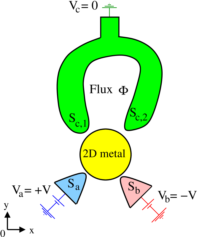
Figure 1: The four-terminal superconducting device: The superconducting leads $S_{a}$, $S_{b}$ and $S_{c}$ are voltage-biased at $(V_{a},V_{b},V_{c})$, with $V_{a}=-V_{b}\equiv V$ on the quartet line and $S_{c}$ is grounded at $V_{c}=0$. The loop in $S_{c}$ terminates at the contact points $S_{{c_{1}}}$ and $S_{{c_{2}}}$ on the 2D metal used to describe the sheet of graphene gated away from the Dirac points in the Harvard group experiment Harvard-group-experiment . The loop is threaded by the magnetic flux $\Phi$.

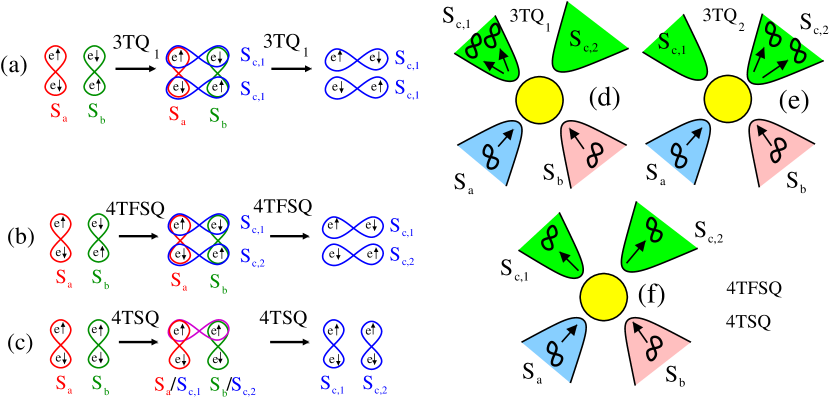
Figure 2: Artist view of the microscopic processes: The three-terminal quartets (3TQ₁, panels a and d), the 3TQ₂ (panel e), the four-terminal statistical fluctuations of the split quartet current (4TFSQ, panel b and f) and the four-terminal split quartets (4TSQ, panel c and f). The two pairs taken from $S_{a}$ and $S_{b}$ biased at $\pm V$ exchange partners according to the “intermediate state” represented schematically on panels a, b and c for the three-terminal 3TQ₁ and the four-terminal 4TFSQ and 4TSQ respectively. Two Cooper pairs are transmitted together into $S_{{c_{1}}}$ (3TQ₁ on panels a and d), or into $S_{c,2}$ (3TQ₂ on panel e). Alternatively, a single Cooper pair is transmitted into $S_{{c_{1}}}$ and another one into $S_{{c_{2}}}$ by the four-terminal 4TFSQ on panels b and f, and by the 4TSQ on panels c and f. A four-particle resonance is produced for the 3TQ and the 4TFSQ on panels a and b, i.e. the two Cooper pairs from $S_{a}$ and $S_{b}$ recombine after exchanging partners. The 4TSQ on panel c involve interchanging a quasiparticle “surfing” on the quantum wake between the $S_{c,1}$ and $S_{c,2}$ contacts, from two Cooper pairs originating from $S_{a}$ and $S_{b}$. The microscopic mechanism is different for the 3TQ and the 4TFSQ (panels a and b), or for the 4TSQ (panel c).

The four-terminal Josephson junction in figure 1 is an opportunity for investigating interference in the quartet current, in the spirit of a superconducting quantum interference device (SQUID)SQUID . Several experiments on multiterminal devices containing loops have been proposed recently Rech ; Pillet ; Pillet2 in absence of voltage biasing, i.e. at equilibrium, where all parts of the circuit are grounded.

The device on figure 1 was proposed recently Nazarov1 ; Nazarov2 to probe Weyl points and nontrivial topology. The voltage biasing conditions are different in Refs. Nazarov1, ; Nazarov2, for topology and Refs. Freyn, ; Melin1, for the quartets: the voltages are incommensurate in Refs. Nazarov1, ; Nazarov2, , so as to sweep the $(\varphi_{a},\varphi_{b})$ Brillouin zone of the superconducting phases. Experiments related to the theoretical proposal on topology Nazarov1 ; Nazarov2 were attempted recently manip-topology1 ; manip-topology2 ; manip-topology3 .

Coming back to the Harvard group experiment Harvard-group-experiment , the emergence of quartet anomaly in four-terminal configurations naturally raises the question of making the theory of the quartets with four terminals, instead of three terminals in the previous theoretical Freyn ; Jonckheere ; Rech ; Melin1 ; Melin2 ; Melin3 ; Melin-finite-frequency-noise ; Doucot and experimental Lefloch ; Heiblum investigations. In this sequence of papers I, II and III, the $(S_{a},S_{b},S_{{c_{1}}},S_{{c_{2}}})$ four-terminal device is biased at $(V_{a},V_{b},V_{c},V_{c})$, where $V_{c}=0$ is the reference voltage of the grounded $S_{c}$ containing a loop threaded by the magnetic flux $\Phi$ and terminated by $S_{{c_{1}}}$ and $S_{{c_{2}}}$ (see figure 1). Our strategy in this series of papers is to develop a theory which is intended to interpret the following unexpected features reported by the Harvard group Harvard-group-experiment :

(i) A quartet Josephson anomaly appears on the $V_{a}+V_{b}=0$ quartet line, once one of the elements of the conductance matrix is plotted in color as a function of the $(V_{a},V_{b})$ voltages Harvard-group-experiment . This is compatible with the theoretical prediction of the quartets for three superconducting terminalsFreyn ; Melin1 , and with the previous Grenoble Lefloch and Weizmann Institute Heiblum group experiments.

(ii) In addition, the four-terminal Harvard group experiment Harvard-group-experiment demonstrates oscillations of the quartet current as a function of the reduced flux $\Phi/\Phi_{0}$ in the loop.

(iii) An “inversion” appears Harvard-group-experiment in a low bias voltage window, if the experimental data for the amplitude of the quartet anomaly are plotted as a function of $\Phi/\Phi_{0}$. Namely, the quartet anomaly is stronger at $\Phi/\Phi_{0}=1/2$ than at $\Phi/\Phi_{0}=0$ even if superconductivity should naively be stronger at $\Phi/\Phi_{0}=0$ than at $\Phi/\Phi_{0}=1/2$. The following paper I addresses a theoretical description of “Inversion in $I_{c}(\Phi/\Phi_{0})$ between $\Phi/\Phi_{0}=0$ and $\Phi/\Phi_{0}=1/2$” on the basis of perturbation theory in the tunnel amplitudes within the simplest $V=0^{+}$ adiabatic limit. In addition, the model is generalized beyond the perturbative and adiabatic regimes.

(iv) Gating away from the Dirac point in the Harvard group experiment Harvard-group-experiment favors $\pi$-periodicity of $I_{c}(\Phi/\Phi_{0})$ with respect to $2\pi$-periodicity. The following paper I turns out to be compatible with this observation.

(v) A small voltage scale $V_{*}$ emergesHarvard-group-experiment in the bias voltage $V$-dependence of the quartet signal. Paper II addresses how inversion is produced by increasing the bias voltage $V$ on the quartet line, in the simple situation of a 0D quantum dot. Paper III addresses whether a “Floquet mechanism” similar to that of paper II can extrapolate to the 2D metal of paper I, in connection with answering the question of why the voltage $V_{*}$ for the inversion is much smaller than the gap in the Harvard group experiment Harvard-group-experiment .

In short, the progression between the three papers is about different levels of the modeling: Paper I starts from the four-terminal split quartets (4TSQ) treated in perturbation in the tunnel amplitudes and in the $V=0^{+}$ adiabatic limit with a 2D metal. Paper I also addresses how the nonstandard four-terminal quartets can be generalized to arbitrary device parameters. Paper II addresses the full Floquet theory at finite bias voltage for a zero-dimensional (0D) quantum dot, i.e. how the Floquet spectra and populations can produce inversion in $I_{c}(\Phi/\Phi_{0})$ between $\Phi/\Phi_{0}=0$ and $\Phi/\Phi_{0}=1/2$. Paper III combines papers I and II and addresses finite bias voltage for a 2D metal of paper I within physically-motivated approximations.

The results of the following paper I which are not presented as theoretical support in the experimental Harvard group paperHarvard-group-experiment are the following:

(i) Rigorous microscopic calculation for the sign and the amplitude of the critical currents through a 2D metal within perturbation theory in the tunnel amplitudes and in the adiabatic limit, taking disorder in the superconducting leads in the dirty limit into account.

(ii) Physically-motivated approximations for addressing the nonstandard 4TSQ at arbitrary interface transparencies and finite bias voltage.

In the following paper I, we propose a simple model for the Harvard group experiment Harvard-group-experiment (see sections III,  IV,  V, VI and VII), and next, the model is analyzed in connection with this experiment (see sections VIII, IX and X).

The detailed structure of paper I is this following. Section II summarizes the three papers of the series. The model and the methods are presented in sections III and IV respectively. The three-terminal 3TQ and the four-terminal 4TSQ current-phase relations are next calculated from perturbation theory in the tunnel amplitudes combined to the adiabatic limit, see section V. Section VI deals with the interference between the three-terminal 3TQ and the four-terminal 4TSQ. The importance of two space dimensions is pointed out in section VII, in connection with the 2D quantum wake. Section VIII shows that “Relative shift of $\pi$ between the three-terminal 3TQ and the four-terminal 4TSQ” implies “Inversion in the critical current $I_{c}(\Phi/\Phi_{0})$ between the reduced flux values $\Phi/\Phi_{0}=0$ and $\Phi/\Phi_{0}=1/2$”. The consequence of the model for the gate voltage dependence of the magnetic field oscillations is discussed in section IX in connection with the Harvard group experimental paper Harvard-group-experiment . Section X discusses arbitrary interface transparencies and finite bias voltage within the proposed approximations. A summary and final remarks are provided in section XI.

II The three papers of the series

In this section, we present the three papers of the series. Specifically, the following items (A), (B) and (C) detail which features of the Harvard group experiment Harvard-group-experiment will be addressed and explained in which paper I, II or III.

(A) The following “paper I” starts with the simplest predictive approach, i.e. perturbation theory in the interface transparencies in the adiabatic limit where $(S_{a},S_{b},S_{{c_{1}}},S_{{c_{2}}})$ are biased at $(V,-V,0,0)$ on the quartet line, with $V=0^{+}$. In the context of Cooper pair splitting in a three-terminal normal metal-superconductor-normal metal ($NSN$) device, similar perturbative approach Hekking ; Melin-Feinberg turned out to usefully uncover the important elementary processes of “elastic cotunneling” Hekking ; Melin-Feinberg and “crossed Andreev reflection” Hekking ; Feinberg ; Melin-Feinberg . Concerning the four-terminal Josephson junction on figure 1, the following perturbative calculations reveal the 3TQ Freyn ; Melin1 interfering with the nonstandard 4TSQ.

More precisely, perturbation theory and the adiabatic limit lead to the three processes which are shown in figure 2:

(a) The three-terminal 3TQ₁, 3TQ₂ in which two pairs (from $S_{a}$ and from $S_{b}$ biased at $\pm V$ respectively) exchange partners and recombine as two outgoing pairs transmitted at the same contact with $S_{{c_{1}}}$ for the 3TQ₁ (or at the contact with $S_{{c_{2}}}$ for the 3TQ₂), see figures 2a, d and e.

(b) The four-terminal statistical fluctuations of the split quartets (4TFSQ) take one pair from $S_{a}$, another one from $S_{b}$ biased at $\pm V$ respectively. Both of them split and recombine as one pair transmitted into $S_{{c_{1}}}$ and another one into $S_{{c_{2}}}$, see figures 2b and f. The 4TFSQ solely contribute to small sample-to-sample statistical fluctuations of the supercurrent.

(c) The four-terminal split quartets (4TSQ) exchange a quasiparticle between two pairs taken from $S_{a}$ and $S_{b}$ biased at $\pm V$ respectively. The 4TSQ realize a “four-terminal quartet beam splitter”, namely, they take two pairs from $S_{a}$ and $S_{b}$, make their wave-function overlap and transmit a pair into $S_{{c_{1}}}$ and another one into $S_{{c_{2}}}$ in the outgoing state, see figures 2c and f. Contrary to the 4TFSQ of the previous item (b), the four-terminal 4TSQ turn out to be robust against averaging their critical current in the presence of multichannel contacts.

It is demonstrated that the three-terminal 3TQ₁, 3TQ₂ (see the above item a ) and the four-terminal 4TSQ (the above item c) are $\pi$- and $0$-shifted respectively, due to the minus sign in the wave-function of a Cooper pair for the former, and to the additional exchange of two quasiparticles via the quantum wake for the latter. The critical current is larger at $\Phi/\Phi_{0}=1/2$ than at $\Phi/\Phi_{0}=0$, i.e. the model of this paper I produces the inversion between $\Phi/\Phi_{0}=0$ and $\Phi/\Phi_{0}=1/2$ which is also obtained in the Harvard group experiment Harvard-group-experiment .

In addition, an approximation on disorder is implemented to address general values of the parameters, i.e. finite bias voltage on the quartet line and arbitrary interface transparencies.

Now, we provide items (B) and (C) summarizing the goals of papers II and III of this series, in connection with explaining the Harvard group experimentHarvard-group-experiment :

(B) We propose in the next paper II a “Floquet level and population mechanism” by which an inversion between $\Phi/\Phi_{0}=0$ and $\Phi/\Phi_{0}=1/2$ is produced by tuning the bias voltage $V$ on the quartet line. Most of the description in this paper II is based on a simplified 0D quantum dot configuration supporting a single level at zero energy. The paper II relies on a combination of analytical theory and extensive numerical calculations. An interesting link is established in paper II, which relates the inversion in the critical current between $\Phi/\Phi_{0}=0$ and $\Phi/\Phi_{0}=1/2$ to repulsion between the Floquet levels as a function of the bias voltage $V$ on the quartet line. Robustness of the inversion is established with respect to crossing-over from weak to strong Landau-Zener tunneling by changing the couplings between the dot and the superconducting leads, and with respect to introducing several energy levels in a multilevel quantum dot. It turns out that the complementary “Floquet mechanism” of paper II for the inversion tuned by the voltage $V$ is different in nature from what is proposed here in the paper I.

(C) The last paper III of the series “merges” the papers I and II into an approximation scheme for the effect of bias voltage within the model proposed here in paper I. A link is established to the proximity effect, however taking the specificities of the three- and four-terminal 3TQ and 4TSQ through a 2D metal into account. In order to illustrate this point, let us consider a two-terminal normal metal-superconductor ($NS$) Andreev interferometer containing a loop in its $N$ part. Electrons with charge $-e$ from $N$ are Andreev-reflected as holes with charge $e$ and a Cooper with charge $-2e$ is transmitted into $S$. Doubling the charge for the quartet mechanism, a pair of electron-like quasiparticles with charge $-2e$ can be reflected as a pair of hole-like quasiparticles with charge $2e$ while two Coopers with charge $-4e$ are transmitted into $S_{c}$. We investigate in paper III whether this can produce inversion in the critical current on the quartet line between $\Phi/\Phi_{0}=0$ and $\Phi/\Phi_{0}=1/2$ (for instance in connection with figure 3c in Ref. Nazarov-electroflux, ). In addition, we obtain emergence of a small energy scale which is compatible with the observation Harvard-group-experiment of a small voltage scale $V_{*}$ in the variations of the critical current with bias voltage $V$.

The above items (A), (B) and (C) summarize the main motivations for investigating the three complementary mechanisms of papers I, II and III. Now, we come specifically to the following paper I.

III The model

This section presents the model of the following paper I. The Hamiltonians are provided in subsection III.1. The voltage biasing conditions are given in subsection III.2. The critical current on the quartet line is defined in subsection III.3, in connection with making the link between our calculations and the Harvard group experiment Harvard-group-experiment .

III.1 The Hamiltonians

The assumptions of the model are presented in this subsection. The essential features of the Harvard group experiment Harvard-group-experiment are listed in subsection III.1.1. The Hamiltonians are presented next, first the BCS Hamiltonian of the superconducting leads (see subsection III.1.2), next the Hamiltonian of the 2D metal used to model the sheet of graphene (see subsection III.1.3), and finally the term of the Hamiltonian describing the contacts between the 2D metal and the superconducting leads (see subsection III.1.4).

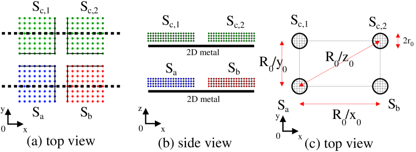
Figure 3: The four-terminal superconducting device: Panel a shows a schematic top view of the Harvard group device Harvard-group-experiment , with four superconducting terminals $S_{a}$, $S_{b}$, $S_{c,1}$ and $S_{c,2}$ evaporated on top of the sheet of graphene which is in the $(x,y)$ plane of the figure . The grounded loop connecting $S_{c,1}$ to $S_{c,2}$ is not shown on panel a. Panel b shows cuts in the $(y,z)$ plane along the dashed lines on panel a. Panel c shows in the $(x,y)$ plane a schematic top view of the geometry considered in this paper I, with superconducting contacts having radius $r_{0}$, which can be smaller or larger than the zero-energy dirty-limit BCS coherence length. The separation between the superconducting contacts is $R_{0}/x_{0}$ along $x$-axis, $R_{0}/y_{0}$ along $y$ axis and $R_{0}/z_{0}$ along the diagonals. The superconducting leads $S_{a}$ and $S_{b}$ are biased at $\pm V$ while $S_{c,1}$ and $S_{c,2}$ belong to the same superconducting loop defined in $S_{c}$ which is grounded at $V_{c}=0$ and contains a loop pierced by flux $\Phi$, see figure 1.

III.1.1 The essential ingredients

We start with presenting which ingredients of the Harvard group experiment Harvard-group-experiment are important to our theoretical description. The model relies on the following facts:

(i) The superconductors are connected on a 2D metal which consists of graphene gated away from the Dirac point, see figures 1 and 3.

(ii) The experiment involves four terminals instead of three in the previous theoretical Freyn ; Jonckheere ; Rech ; Melin1 ; Melin2 ; Melin3 ; Melin-finite-frequency-noise ; Doucot and experimental Lefloch ; Heiblum papers, see figures 1 and 3.

The discussion starts with two limiting cases for the device parameters:

(a) The limit of low-transparency interfaces between the 2D metal and the superconducting leads.

(b) The $V=0^{+}$ adiabatic limit with voltage-biasing on the quartet line.

The theory is next generalized to arbitrary interface transparencies and finite bias voltage within a physically motivated approximation regarding disorder.

The assumptions about the geometry are illustrated in figure 3. Panels a and b show the geometry of the Harvard group experiment Harvard-group-experiment , with four superconducting contacts $S_{a}$, $S_{b}$, $S_{c,1}$ and $S_{c,2}$ evaporated on top of the sheet of graphene. Panel a shows top view of the experimental configuration in the plane of the $(x,y)$-coordinates. Panel b shows side views in the $(y,z)$-plane, i.e. cuts along the dashed lines on panel a. Figure 3c represents the $(x,y)$-plane top view of the model considered in this paper I, in which four superconducting leads $S_{a}$, $S_{b}$, $S_{c,1}$ and $S_{c,2}$ form contacts of radius $r_{0}$ on the 2D metal, where $r_{0}$ can be smaller or larger than the zero-energy dirty-limit BCS coherence length. The separation between the contacts on figure 3c corresponds to the parameters $R_{0}/x_{0}$ and $R_{0}/y_{0}$ along the $x$- and $y$-axis directions respectively, and to $R_{0}/z_{0}$ along the diagonals.

III.1.2 BCS Hamiltonian of the superconducting leads

Now, we present the standard BCS Hamiltonian of each superconducting lead taken individually. In zero flux $\Phi/\Phi_{0}=0$, all superconducting leads are described by

$${\cal H}_{BCS} = -W\sum_{\langle i,j\rangle}\sum_{\sigma=\uparrow,\downarrow}\left(c_{i,\sigma}^{+}c_{j,\sigma}+c_{j,\sigma}^{+}c_{i,\sigma}\right)$$ (8)

$$- \Delta\sum_{i}\left(e^{i\varphi}c_{i,\uparrow}^{+}c_{i,\downarrow}^{+}+e^{-i\varphi}c_{i,\downarrow}c_{i,\uparrow}\right),$$ (9)

where the summation $\sum_{\langle i,j\rangle}$ runs over the pairs of nearest neighbors on a 3D tight-binding cubic lattice while $\sum_{i}$ runs over the tight-binding sites. The notation $\sigma=\uparrow,\downarrow$ stands for the spin. The first term in Eq. (8) is the kinetic energy. The second term given by Eq. (9) is the BCS mean field pairing with superconducting gap $\Delta$. The macroscopic superconducting phase variable is generically denoted by $\varphi$ in Eq. (9), and it takes the values $\varphi_{a}$, $\varphi_{b}$, $\varphi_{c,1}$ or $\varphi_{c,2}$ according to which of the superconducting lead $S_{a}$, $S_{b}$, $S_{c,1}$ or $S_{c,2}$ is considered.

A magnetic field in the loop is taken into account in the following gauge:

$$\varphi_{c,\,1} = \varphi_{c}-\frac{\Phi}{2}$$ (10)

$$\varphi_{c,\,2} = \varphi_{c}+\frac{\Phi}{2},$$ (11)

with a phase gradient along the loop $S_{c}$ terminated by $S_{{c_{1}}}$ and $S_{{c_{2}}}$, supposed to have perimeter large compared to the superconducting coherence length.

III.1.3 Hamiltonian of the 2D metal

Now, the 2D metal Hamiltonian is presented, see the yellow region on figure 1:

$${\cal H}_{2D\,metal}=-W\sum_{\langle i,j\rangle}\sum_{\sigma=\uparrow,\downarrow}\left(c_{i,\sigma}^{+}c_{j,\sigma}+c_{j,\sigma}^{+}c_{i,\sigma}\right),$$ (12)

where the summation $\sum_{\langle i,j\rangle}$ runs over pairs of neighbors on a 2D tight-binding lattice.

In the following calculations, the 2D metal is considered to be infinite in the $x$- and $y$-axis directions, which is compatible with the large sheet of graphene used in Harvard group experiment Harvard-group-experiment , having typical dimension $\sim 10\,\mu$m.

We simply take the continuum limit for a 2D Fermi gas with circular Fermi surface, parameterized by the single Fermi wave-vector $k_{F}$ and the band-width $W$. The assumption of circular Fermi surface can be realized approximately from the generic tight-binding Hamiltonians given by Eq. (12) at low or high filling, and it provides a useful phenomenological basis for describing a sheet of graphene gated away from the Dirac point, with a minimal number of parameters and only two essential ingredients: spin-$1/2$ fermions and 2D.

In spite of its simplicity, it turns out that this circular Fermi surface 2D Fermi gas Hamiltonian will be well suited for addressing how the gate voltage on the sheet of graphene in the Harvard group experiment Harvard-group-experiment couples to the signal on the quartet line. Approaching the Dirac points with gate voltage could be interesting for future experiments, which would require taking into account the additional ingredient of the full dispersion relation of graphene, including the Dirac cones.

III.1.4 Tunneling between the superconductors and the 2D metal

Now, we present the tunnel Hamiltonian between the 2D metal and each of the superconducting lead $S_{N}$ among $\{S_{a},S_{b},S_{c_{1}},S_{c_{2}}\}$. This coupling Hamiltonian consists of hopping between both sides of the junction:

$${\cal H}_{T,\,N}=-J_{N}\sum_{\langle i_{N},j_{N}\rangle}\sum_{\sigma=\uparrow,\downarrow}\left(c_{j_{N},\sigma}^{+}c_{i_{N},\sigma}+c_{i_{N},\sigma}^{+}c_{j_{N},\sigma}\right),$$ (13)

where the summation $\sum_{\langle i_{N},j_{N}\rangle}$ runs over the pairs of sites on both sides of the interfaces.

The notations used throughout the paper for labeling the interfaces between the 2D metal and the four $S_{a}$, $S_{b}$, $S_{c,1}$ and $S_{c,2}$ superconducting leads are the following: We denote by $a_{p}$, $b_{p}$, $c_{1,p}$ and $c_{2,p}$ the tight-binding sites on the superconducting side of the contacts, and by $\alpha_{p}$, $\beta_{p}$, $\gamma_{c_{1},p}$ and $\gamma_{c_{2},p}$ their counterpart on the 2D metal.

III.2 Voltage biasing conditions

The voltage biasing conditions are made explicit in this subsection. The four-terminal $(S_{a},S_{b},S_{{c_{1}}},S_{{c_{2}}})$ device in figure 1 is voltage-biased on the quartet line at $(V_{a},V_{b},V_{c},V_{c}),$ with $V_{a}=-V_{b}\equiv V$ and $V_{c}=0$. We implement the $V=0^{+}$ adiabatic limit combined to perturbation theory in $\{J_{N}\}$ in the following sections V , VI, VII.3, VIII and IX, see Eq. (13) for $J_{N}$. In addition, section X addresses the more general conditions of finite bias voltage $V$ on the quartet line and arbitrary interface transparencies, within the physically-motivated approximation for disorder introduced in section IV.4.

III.3 A relevant physical quantity

In this subsection, we present the definition of the critical current on the quartet line. This quantity is measured in the Harvard group experiment Harvard-group-experiment , and it is evaluated theoretically in the following papers I, II and III. The “critical current on the quartet line” $I_{c}(V,\Phi/\Phi_{0})$ is called in short as “the critical current”:

$$I_{c}(V,\Phi/\Phi_{0})=\mbox{Max}_{\varphi_{q,\,3T}}I_{S}(\varphi_{q,\,3T},V,\Phi/\Phi_{0}),$$ (14)

where $I_{c}(V,\Phi/\Phi_{0})$ is gauge-invariant and the quartet phase $\varphi_{q,\,3T}$-sensitive $I_{S}(\varphi_{q,\,3T},V,\Phi/\Phi_{0})$ can be calculated in any gauge. This is why it is legitimate to use the specific gauge given by Eqs. (10)-(11).

IV The methods

This section introduces the methods used in this paper I. The calculation of the currents is presented in subsection IV.1. Subsection IV.2 deals with their perturbative expansion in the tunnel amplitudes. Superconducting diffusion modes are next introduced in subsection IV.3. Subsection IV.4 presents the approximations on disorder which will be used in section X to address arbitrary interface transparencies and finite bias voltage on the quartet line.

IV.1 Calculation of the current

This subsection explains the method to evaluate the currents from the Keldysh Green’s functions. Subsection IV.1.1 presents the bare Green’s functions in absence of the tunnel coupling between the different leads. The Dyson equations are next presented in subsection IV.1.2. Subsection IV.1.3 deals with how the current is expressed with Keldysh Green’s function. The transport formula is next specialized to the equilibrium and adiabatic limits in subsection IV.1.4.

IV.1.1 Bare Green’s functions

In this subsection, we present the Green’s functions in absence of the tunnel coupling between the different parts of the circuit, i.e. the bare Green’s functions with $J_{N}=0$ in Eq. (13).

The two-component Bogoliubov-de Gennes wave-functions for spin-up electrons and spin-down holes yield $2\times 2$ matrix advanced (or retarded) Green’s function describing propagation between the tight-binding sites ${\bf x}_{1}$ and ${\bf x}_{2}$ at times $t_{1}$ and $t_{2}$:

$$\hat{g}^{A}_{{\bf x}_{1},{\bf x}_{2}}(t_{1},t_{2})=-i\theta(t_{1}-t_{2})$$ (15)

$$\left(\begin{array}[]{cc}\langle\left\{c_{{\bf x}_{1},\uparrow}(t_{1}),c^{+}_{{\bf x}_{2},\uparrow}(t_{2})\right\}\rangle&\langle\left\{c_{{\bf x}_{1},\uparrow}(t_{1}),c_{{\bf x}_{2},\downarrow}(t_{2})\right\}\rangle\\ \langle\left\{c^{+}_{{\bf x}_{1},\downarrow}(t_{1}),c^{+}_{{\bf x}_{2},\uparrow}(t_{2})\right\}\rangle&\langle\left\{c^{+}_{{\bf x}_{1},\downarrow}(t_{1}),c_{{\bf x}_{2},\downarrow}(t_{2})\right\}\rangle\end{array}\right),$$ (18)

where $\left\{A,B\right\}=AB+BA$ is an anticommutator between the fermionic creation or annihilation operators $A$ and $B$. Eq. (15) is useful in connection with the Dyson equations, and it can be used to address the time-periodic dynamics underlying the emergence of a dc-current of quartetsFreyn ; Melin1 , as well as arbitrary device parameters (i.e. arbitrary interface transparencies and finite bias voltage on the quartet line).

Considering the 2D metal [see the Hamiltonian given by Eq. (12), taken at low or high filling] and Fourier transforming from the time variables $t_{1}$ and $t_{2}$ to frequency $\omega$, Eqs. (152)-(153) in Appendix A imply the following limiting long-distance behavior of the Green’s function for $k_{F}R\gg 1$:

$$g^{A,(1,1)}_{2D\,metal}(R,\omega) = g^{A,(2,2)}_{2D\,metal}(R,\omega)$$ (19)

$$\simeq \frac{i}{W\sqrt{k_{F}R}}\cos\left(k_{F}R-\frac{\pi}{4}\right)$$ (20)

$$g^{R,(1,1)}_{2D\,metal}(R,\omega) = g^{R,(2,2)}_{2D\,metal}(R,\omega)$$ (21)

$$\simeq -\frac{i}{W\sqrt{k_{F}R}}\cos\left(k_{F}R-\frac{\pi}{4}\right),$$ (22)

where the $(1,1)$ and $(2,2)$ labels in the superscript denote the Nambu “spin-up electron” and “spin-down hole” components respectively. The notation $R=|{\bf x}_{1}-{\bf x}_{2}|$ stands for the separation between ${\bf x}_{1}$ and ${\bf x}_{2}$ in real space. Eqs. (19)-(22) assume that the separations $R_{0}/x_{0}$, $R_{0}/y_{0}$ and $R_{0}/z_{0}$ between the contacts are small compared to the zero-energy ballistic-limit coherence length given by Eq. (5), see figure 3 for the notations $R_{0}/x_{0}$, $R_{0}/y_{0}$ and $R_{0}/z_{0}$. Taking the short-junction limit $\Delta R/v_{F}\ll 1$ amounts to substituting the electron and hole wave-vectors $k=k_{e}$ and $k=k_{h}$ in Eqs. (19)-(20) and Eqs. (21)-(22) respectively with the Fermi wave-vector $k_{F}$, without accounting for their different energy-$\omega$ dependence $k_{e,h}=k_{F}\pm\omega/v_{F}$.

A sanity check of Eqs. (19)-(22) is provided in section I of the Supplemental Material supplemental , for a double junction between a 2D normal metal and 3D normal leads. In particular, it is mentioned at the end of section I in the Supplemental Material supplemental that Eqs. (19)-(22) imply the magnetic proximity effect at a 2D metal-3D ferromagnet interface, namely, a magnetization in induced in the 2D metal.

Considering now the superconducting leads [see the Hamiltonian given by Eqs. (8)-(9)], the ballistic nonlocal Green’s function of the 3D superconductor $S_{N}$ with gap $\Delta$ and phase $\varphi_{N}$ is the following:

$$\hat{g}^{A}_{{\bf x}_{1},{\bf x}_{2}}(\omega)=\frac{1}{W}\frac{1}{k_{F}R}\exp\left\{\left(-\frac{\left|{\bf x}_{1}-{\bf x}_{2}\right|}{\xi_{ball}(\omega-i\eta)}\right)\right\}$$

$$\left[\frac{\sin(k_{F}R)}{\sqrt{\Delta^{2}-(\omega-i\eta)^{2}}}\left(\begin{array}[]{cc}-(\omega-i\eta)&\Delta e^{i\varphi_{N}}\\ \Delta e^{-i\varphi_{N}}&-(\omega-i\eta)\end{array}\right)\right.$$ (25)

$$\left.\left.+\cos(k_{F}R)\left(\begin{array}[]{cc}-1&0\\ 0&1\end{array}\right)\right]\right\}.$$ (28)

The Dynes parameter $\eta\ll\Delta$ is viewed as a requirement for making the difference between the “advanced” and “retarded” Green’s functions, or as a phenomenological parameter to capture the experimental line-width broadening and relaxation in superconductorsMelin3 ; Kaplan ; Dynes ; Pekola1 ; Pekola2 . In addition, the ballistic-limit BCS coherence length appearing in Eq. (25) is given by

$$\xi_{ball}(\omega-i\eta)=\frac{\hbar v_{F}}{\sqrt{\Delta^{2}-(\omega-i\eta)^{2}}},$$ (29)

which goes to Eq. (5) if $\omega-i\eta\rightarrow 0$.

At equilibrium i.e. if $V=0$, the hopping amplitude $\hat{J}_{N}$ between the 2D metal and the superconducting lead $S_{N}$ is given by the diagonal $2\times 2$ Nambu matrix

$$\hat{J}_{N}=\left(\begin{array}[]{cc}J_{N}&0\\ 0&-J_{N}\end{array}\right).$$ (30)

IV.1.2 Dyson equations at equilibrium

Now, we consider $J_{N}\neq 0$ in Eq. (30) and start with equilibrium conditions, i.e. all leads are grounded at $V=0$ and the superconductors are phase-biased. All parts of the circuit then have identical chemical potential taken as the energy reference.

The fully dressed advanced and retarded Green’s functions $\hat{G}^{A}$ and $\hat{G}^{R}$ describe the 2D metal connected by finite hopping amplitudes $\{\hat{J}_{N}\}$ to the superconducting leads. Their values are obtained from the Dyson equations, which take the following form in a compact notation:

$$\hat{G}^{A,R}=\hat{g}^{A,R}+\hat{g}^{A,R}\otimes\hat{J}\otimes\hat{G}^{A,R},$$ (31)

where the symbol $\otimes$ is a convolution over time variables [such the time variables $t_{1}$ and $t_{2}$ in Eq. (15)] which becomes a simple product after Fourier transforming to the frequency/energy $\omega$. A summation over all possible tight-binding sites between the 2D metal and the superconducting leads is carried out according to

$$\hat{G}^{A,R}_{\alpha_{r},\beta_{s}}(\omega) = \hat{g}^{A,R}_{\alpha_{r},\beta_{s}}(\omega)+\sum_{\gamma_{p}}\hat{g}^{A,R}_{\alpha_{r},\gamma_{p}}(\omega)\hat{J}_{\gamma_{p},c_{p}}\hat{G}^{A,R}_{c_{p},\beta_{s}}(\omega)$$ (32)

$$= \hat{g}^{A,R}_{\alpha_{r},\beta_{s}}(\omega)$$

$$+ \sum_{\gamma_{p},\gamma_{q}}\hat{g}^{A,R}_{\alpha_{r},\gamma_{p}}(\omega)\hat{J}_{\gamma_{p},c_{p}}\hat{g}^{A,R}_{c_{p},c_{q}}(\omega)\hat{J}_{c_{q},\gamma_{q}}\hat{G}^{A,R}_{\gamma_{q},\beta_{s}}(\omega),$$

where a closed set of linear equations is obtained at second order for $\{\hat{G}^{A,R}_{\alpha_{r},\beta_{s}}\}$ in Eq. (IV.1.2).

IV.1.3 Finite bias voltage on the quartet line

Finite bias voltage $V\neq 0$ on the quartet line implies a single Josephson frequency $2eV/\hbar$ for the considered four-terminal Josephson junction biased at opposite voltages, see subsection IV.1.3. The periodic time dynamics is encoded in the Nambu tunnel amplitudes between the 2D metal and the superconducting leads $\{S_{N}\}$: Eq. (30) is replaced by

$$\hat{J}_{N}(t)=\left(\begin{array}[]{cc}J_{N}\exp(ieV_{N}t/\hbar)&0\\ 0&-J_{N}\exp(-ieV_{N}t/\hbar)\end{array}\right),$$ (34)

where $V_{N}$ is the voltage $V_{N}=0,\,\pm V$ at which superconducting lead $S_{N}$ is biased. At finite voltage $V$, and after Fourier transforming from time $t$ to frequency $\omega$, the “advanced” and “retarded” Green’s functions in Eq. (31)-(IV.1.2) become infinite matrices having labels in the extended space of the harmonics of the Josephson frequency, in addition to being matrices in Nambu.

The fully dressed Keldysh Green’s function takes the formCaroli ; Cuevas

$$\hat{G}^{+,-}=\left(\hat{I}+\hat{G}^{R}\otimes\hat{J}\right)\otimes\hat{g}^{+,-}\otimes\left(\hat{I}+\hat{J}\otimes\hat{G}^{A}\right).$$ (35)

The “bare” Keldysh Green’s function is given by

$$\hat{g}^{+,-}(\omega)=n_{F}(\omega)\left[\hat{g}^{A}(\omega)-\hat{g}^{R}(\omega)\right],$$ (36)

where $n_{F}(\omega)$ is the Fermi-Dirac distribution function, which reduces to the step function $n_{F}(\omega)=\theta(-\omega)$ in the limit of zero temperature.

The current $I_{\alpha\rightarrow a}$ flowing from the 2D metal to the superconducting lead $S_{a}$ at the $\alpha-a$ contact is given by Caroli ; Cuevas

$$-I_{\alpha\rightarrow a} = \frac{e}{\hbar}\sum_{p}\int d\omega\left\{\left[\hat{J}_{a_{p},\alpha_{p}}\hat{G}^{+,-}_{\alpha_{p},a_{p}}\right]_{(1,1)/(0,0)}(\omega)\right.$$ (40)

$$-\left[\hat{J}_{a_{p},\alpha_{p}}\hat{G}^{+,-}_{\alpha_{p},a_{p}}\right]_{(2,2)/(0,0)}(\omega)$$

$$-\left[\hat{J}_{\alpha_{p},a_{p}}\hat{G}^{+,-}_{a_{p},\alpha_{p}}\right]_{(1,1)/(0,0)}(\omega)$$

$$+\left.\left[\hat{J}_{\alpha_{p},a_{p}}\hat{G}^{+,-}_{a_{p},\alpha_{p}}\right]_{(2,2)/(0,0)}(\omega)\right\},$$

where “$(1,1)$” or “$(2,2)$” in the first pair of labels correspond to the Nambu components, as in the above equations. The notation $(n,m)=(0,0)$ in the second pair of labels denotes the static dc-component in the extended space of the harmonics of the Josephson frequency $(neV/\hbar,meV/\hbar)$. The variable $p$ in Eqs. (40)-(40) runs over the tight-binding sites at the interface between the 2D metal and the superconductors, see figure 3 for the geometry of the contacts. Eqs. (35)-(40) are the starting point of the demonstration of the generalized Ambegaokar-Baratoff formula at finite bias voltage $V$ on the quartet line, see the forthcoming subsection X.2.1.

IV.1.4 Specializing to equilibrium and the adiabatic limit

Now, we come back to the equilibrium limit $V=0$. The Keldysh Green’s function given by Eq. (35) simplifies as

$$G^{+,-}_{eq}(\omega)=n_{F}(\omega)\left[\hat{G}^{A}(\omega)-\hat{G}^{R}(\omega)\right].$$ (41)

Inserting Eq. (41) into Eqs. (40)-(40) for the current as a function of $\hat{G}^{+,-}$ leads to the equilibrium current though the multichannel “$\alpha,a$” contact:

$$-I_{\alpha\rightarrow a,eq}=\frac{e}{\hbar}\sum_{p}\int d\omega n_{F}(\omega)\left\{\right.$$

$$\left.\left[\hat{J}_{a_{p},\alpha_{p}}\left(\hat{G}^{A}_{\alpha_{p},a_{p}}-\hat{G}^{R}_{\alpha_{p},a_{p}}\right)\right]_{(1,1)}(\omega)\right.$$ (42)

$$-\left[\hat{J}_{a_{p},\alpha_{p}}\left(\hat{G}^{A}_{\alpha_{p},a_{p}}-\hat{G}^{R}_{\alpha_{p},a_{p}}\right)\right]_{(2,2)}(\omega)$$ (43)

$$-\left[\hat{J}_{\alpha_{p},a_{p}}\left(\hat{G}^{A}_{a_{p},\alpha_{p}}-\hat{G}^{R}_{a_{p},\alpha_{p}}\right)\right]_{(1,1)}(\omega)$$ (44)

$$+\left.\left[\hat{J}_{\alpha_{p},a_{p}}\left(\hat{G}^{A}_{a_{p},\alpha_{p}}-\hat{G}^{R}_{a_{p},\alpha_{p}}\right)\right]_{(2,2)}(\omega)\right\},$$ (45)

where $\alpha_{p}$ and $a_{p}$ label the tight-binding sites on the 2D metal and superconducting sides respectively. Eqs. (42)-(45) are the starting point of the perturbative expansion of the current in powers of $J_{0}/W$, see the forthcoming section V.

The matrices $\hat{J}$ [defined by Eq. (30)] and $\hat{G}$ [defined by Eq. (31)] appearing in Eq. (42)-(45) are $2\times 2$ in Nambu, and the “$(1,1)$” or “$(2,2)$ Nambu components of their product is evaluated according to the labels in the subscript.

The equilibrium current $I_{\alpha\rightarrow a,eq}$ given by Eqs. (42)-(45) depends on all superconducting phase variables $\varphi_{a}$, $\varphi_{b}$, $\varphi_{c_{1}}$ and $\varphi_{c_{2}}$. Gauge invariance implies that

$$I_{\alpha\rightarrow a,eq}=I_{\alpha\rightarrow a}\left(\varphi_{a}+\alpha,\varphi_{b}+\alpha,\varphi_{c_{1}}+\alpha,\varphi_{c_{2}}+\alpha\right)$$ (46)

is independent on $\alpha$ because a global superconducting phase is not measurable.

At finite bias voltage $V$ on the quartet line, the phase variables are given by $\varphi_{a}=\varphi^{(0)}_{a}+\psi$, $\varphi_{b}=\varphi^{(0)}_{a}-\psi$, $\varphi_{c_{1}}=\varphi_{c_{1}}^{(0)}$ and $\varphi_{c_{2}}=\varphi_{c_{2}}^{(0)}$, where $\psi=2eVt$ is linear in the time variable $t$. Assuming in addition adiabatic voltage biasing at $V=0^{+}$ leads to slow time-dependence of the variable $\psi$. Then, the adiabatic-limit current is obtained by averaging Eq. (46) over $\psi$:

$$I_{\alpha\rightarrow a,adiab}=\int\frac{d\psi}{2\pi}$$ (47)

$$I_{\alpha\rightarrow a}\left(\varphi_{a}^{(0)}+\psi+\alpha,\varphi_{b}^{(0)}-\psi+\alpha,\varphi_{c_{1}}^{(0)}+\alpha,\varphi_{c_{2}}^{(0)}+\alpha\right).$$

Energy conservation puts the constraint that, on the quartet line, $I_{\alpha\rightarrow a,adiab}$ in Eq. (47) depends only on the gauge-invariant quartet phase variable $\varphi_{q,\,3T}=\varphi_{a}^{(0)}+\varphi_{b}^{(0)}-2\varphi_{c}^{(0)}\equiv\varphi_{a}+\varphi_{b}-2\varphi_{c}$. Gauge invariance implies that the current $I_{\alpha\rightarrow a,adiab}$ is independent on $\alpha$, similarly to the previous Eq. (46) corresponding to equilibrium with $V=0$.

IV.2 Perturbative expansion of the adiabatic current

This subsection presents how the Dyson Eq. (31) is used in the forthcoming section V to produce a systematic expansion of the current in powers of the tunnel amplitudes $\{J_{N}\}$ between the 2D metal and the superconductors $\{S_{N}\}$. Iterating Eq. (31) produces the series

$$G = g$$ (48)

$$+ g\otimes J\otimes g$$ (49)

$$+ g\otimes J\otimes g\otimes J\otimes g$$ (50)

$$+ g\otimes J\otimes g\otimes J\otimes g\otimes J\otimes g$$ (51)

$$+ g\otimes J\otimes g\otimes J\otimes g\otimes J\otimes g\otimes J\otimes g$$ (52)

$$+ g\otimes J\otimes g\otimes J\otimes g\otimes J\otimes g\otimes J\otimes g\otimes J\otimes g$$ (53)

$$+ g\otimes J\otimes g\otimes J\otimes g\otimes J\otimes g\otimes J\otimes g\otimes J\otimes g\otimes J\otimes g$$ (54)

$$+ ...,$$ (55)

which is inserted into Eqs. (42)-(45) for the equilibrium current.

At each order $J_{a}^{2m_{a}}J_{b}^{2m_{b}}J_{{c_{1}}}^{2m_{{c_{1}}}}J_{{c_{2}}}^{2m_{{c_{2}}}}$ in the tunnel amplitudes $\{J_{N}\}$, the expansion given by Eqs. (48)-(55) produces a finite number of “closed loop diagrams” contributing to the dc-current, where $m_{a}$, $m_{b}$, $m_{{c_{1}}}$ and $m_{{c_{2}}}$ are four positive integers.

As seen from Eqs. (42)-(45) and from Eqs. (48)-(55), this diagrammatic expansion has a simple structure, due to the fact that all terms in the Hamiltonian are quadratic, see Eqs. (8)-(9), Eq. (12) and Eq. (13). The diagrams consist of alternations between:

(i) The tunnel amplitudes in and out the 2D metal, see Eq. (30).

(ii) Propagation through the 2D metal [see Eqs. (19)-(22)] or through one of the superconducting leads [see Eq. (25)].

Some of the relevant diagrams are shown schematically on the forthcoming figures 4, 5, 6, 7 and 8.

The equilibrium current is obtained as a series of diagrams which are labeled by the four positive integers $(m_{a},m_{b},m_{{c_{1}}},m_{{c_{2}}})$ mentioned above. Assuming identical tunnel amplitudes $J_{0}\equiv J_{a}=J_{b}=J_{{c_{1}}}=J_{{c_{2}}}$ for all contacts produces the prefactor $(J_{0})^{m}$, with $m=m_{a}+m_{b}+m_{{c_{1}}}+m_{{c_{2}}}$. For instance, the three-terminal 3TSQ₁, 3TQ₂ appear at the order $m=8$, see the forthcoming subsection V.1. The four-terminal 4FTSQ and 4TSQ appear at the order $m=12$, see the forthcoming subsections V.2 and V.3.

Each Green’s function propagating through any superconducting lead $S_{N}$ is within the electron-electron, hole-hole, electron-hole or hole-electron Nambu channel. Each electron-hole or hole-electron conversion produces $\exp\left(\pm i\varphi_{N}\right)$, where $\varphi_{N}$ is the macroscopic phase variable of the superconductor $S_{N}$ (which is among $\{S_{a},S_{b},S_{c_{1}},S_{c_{2}}\}$). To each diagram is thus associated the overall factor

$$\exp\left[i\left(n_{a}\varphi_{a}+n_{b}\varphi_{b}+n_{c_{1}}\varphi_{c_{1}}+n_{c_{2}}\varphi_{c_{2}}\right)\right],$$ (56)

where $(n_{a},n_{b},n_{c_{1}},n_{c_{2}})$ are four (positive or negative) integers counting the number and the sign of the electron-hole or hole-electron conversions in the leads $\{S_{a},S_{b},S_{c_{1}},S_{c_{2}}\}$ respectively, within a given quantum process.

Voltage biasing at $V_{a}=-V_{b}\equiv V$ on the quartet line (see subsection III.2) implies a constraint on $(n_{a},n_{b},n_{c,1},n_{c,2})$ coming from conservation of energy between:

(i) The energy $n_{a}eV_{a}$ of the $n_{a}$ pairs taken from $S_{a}$, and the energy $n_{a}eV_{b}$ of the $n_{b}$ pairs taken from $S_{b}$, and

(ii) The energy $(n_{c_{1}}+n_{c_{2}})eV_{c}=0$ of the $n_{c_{1}}+n_{c_{2}}$ pairs transmitted into $S_{c_{1}}$ and $S_{c_{2}}$ which are both grounded at $V_{c}=0$.

Energy conservation on the quartet line implies $n_{a}eV_{a}+n_{b}eV_{b}=0$ and thus $n_{a}=n_{b}$.

In addition, gauge invariance puts the constraint $n_{a}+n_{b}+n_{c,1}+n_{c,2}=0$, which is compatible with Eqs. (46) and (47) being independent on $\alpha$.

IV.3 The superconducting diffusion modes

Now, we discuss the importance of disorder in the superconductors supposed to be in the dirty limit, i.e. the elastic mean free path $l_{e}$ is much shorter than the ballistic-limit coherence length $\xi_{ball}(0)$ given by Eq. (5). This realistic assumption puts a severe constraints on the diagrammatic perturbation theory: The nonlocal Green’s functions are gathered in a pair-wise manner in a real-space representation, even those crossing the ballistic 2D metal. In addition, small disorder in the 2D metal in the form of nonmagnetic impurities helps gathering the Green’s function in a pair-wise manner. It is likely that the 4TSQ are robust against introducing a small concentration of nonmagnetic impurities in the 2D metal, assuming localization length which is larger than the separation between the contacts. Clarifying this issue in future work requires understanding the fate of the quantum wake in the presence of disorder, see section VII for the quantum wake in the absence of disorder.

Considering a superconductor in the dirty limit, the disorder-averaged single-particle Nambu Green’s function oscillates with the Fermi wave-vector $k_{F}$ [see Eq. (25)] and its envelope decays exponentially over the elastic mean free path Abrikosov . This puts constraint of locality on the “unpaired” single-particle Green’s function at each superconducting lead $S_{N}$.

Second, the superconducting diffusion modes are defined as pairs of single-particle Green’s functions which scatter together on the same realization of the disorder. The range of the superconducting diffusion modes reaches the dirty-limit coherence length at subgap energies, which is much larger than the elastic mean free path for a superconductor such as Aluminum in the dirty limit.

The calculation of the superconducting diffusion modes in the dirty limit generalizes Ref. Smith-Ambegaokar, , see Appendix B. The superconducting diffusion modes have four Nambu labels $(\tau_{1},\tau_{2},\tau_{3},\tau_{4})$ attached to them, see Appendix B. The resulting $2^{4}=16$ terms are provided by Eqs. (B.2.2)-(207). They take the following form in the ladder approximation:

$$\int\frac{d{\bf k}}{(2\pi)^{3}}\overline{g_{\tau_{1},\tau_{2}}({\bf k},\omega)g_{\tau_{3},\tau_{4}}({\bf k}+{\bf q},\omega)}$$

$$= \frac{1}{16\pi W}\frac{1}{2\sqrt{|\Delta|^{2}-(\omega-i\eta)^{2}}+{\cal D}q^{2}}F_{(\tau_{1},\tau_{2})}^{(\tau_{3},\tau_{4})}\left(\frac{\omega-i\eta}{|\Delta|},\varphi_{N}\right),.$$

where ${\bf k}$ and ${\bf q}$ are the wave-vectors, ${\cal D}=v_{F}^{2}\tau/3$ is the diffusion constant with $\tau$ the elastic scattering time, and $\varphi_{N}$ is the superconducting phase variable of the superconducting lead $S_{N}$. The function $F_{(\tau_{1},\tau_{2})}^{(\tau_{3},\tau_{4})}$ appearing in Eq. (IV.3) is deduced from Eqs. (B.2.2)-(207) in Appendix B, for instance:

$$F_{(1,2)}^{(1,2)}\left(\frac{\omega-i\eta}{|\Delta|},\varphi_{N}\right) = \frac{|\Delta|^{2}}{|\Delta|^{2}-(\omega-i\eta)^{2}}\exp\left(2i\varphi_{N}\right)$$ (58)

$$F_{(1,1)}^{(1,2)}\left(\frac{\omega-i\eta}{|\Delta|},\varphi_{N}\right) = \frac{(\omega-i\eta)|\Delta|}{|\Delta|^{2}-(\omega-i\eta)^{2}}\exp\left(i\varphi_{N}\right).$$ (59)

The $\overline{g_{(1,2)}g_{(1,2)}}$ superconducting diffusion mode in Eq. (58) is relevant to the three-terminal 3TQ₁, 3TQ₂. Conversely, $\overline{g_{(1,1)}g_{(1,2)}}$ given by Eq. (59) is relevant to the four-terminal 4TSQ, as well as to the normal metal-superconductor-superconductor ($NSS$) double junction considered in Ref. NSS, . Eq. (58) and Eq. (59) are deduced from the corresponding Eqs. (B.2.2) and (206) in Appendix B.

Fourier transforming Eq. (IV.3) from the wave-vector ${\bf q}$ to the real-space coordinate $R$ leads to

$$\overline{g_{\tau_{1},\tau_{2}}g_{\tau_{3},\tau_{4}}}(R,\omega)=\frac{c}{W^{2}}\left(\frac{\xi_{dirty}(\omega-i\eta)}{l_{e}}\right)$$

$$\times F_{(\tau_{1},\tau_{2})}^{(\tau_{3},\tau_{4})}\left(\frac{\omega-i\eta}{|\Delta|},\varphi_{N}\right)\exp\left(-\frac{R}{\xi_{dirty}(\omega-i\eta)}\right),$$

where $c$ is a constant of order unity and

$$\xi_{dirty}(\omega)\sim\sqrt{l_{e}\xi_{ball}(\omega)}$$ (61)

denotes the superconducting coherence length in the dirty limit.

Next, we integrate Eq. (IV.3) over the separation $R=|{\bf x}_{1}-{\bf x}_{2}|$ between the tight-binding sites ${\bf x}_{1}$ and ${\bf x}_{2}$ at the interface. We distinguish between the following two situations:

(i) If $r_{0}\gtrsim\xi_{dirty}(0)$, then

$$\langle\langle g_{\tau_{1},\tau_{2}}g_{\tau_{3},\tau_{4}}\rangle\rangle\simeq\frac{c^{\prime}}{2W^{2}}\frac{\xi_{dirty}(\omega-i\eta)}{l_{e}}F_{(\tau_{1},\tau_{2})}^{(\tau_{3},\tau_{4})}\left(\frac{\omega-i\eta}{|\Delta|},\varphi_{N}\right),$$ (62)

where the contact radius $r_{0}$ is shown on figure 3c, $\xi_{dirty}(\omega)$ is given by Eq. (61), $c^{\prime}$ is a constant of order unity and $\langle\langle...\rangle\rangle$ stands for summation of $\overline{g_{\tau_{1},\tau_{2}}g_{\tau_{3},\tau_{4}}}$ over the separation $R$ in Eq. (IV.3).

(ii) Conversely, the assumption $r_{0}\lesssim\xi_{dirty}(0)$ leads to

$$\langle\langle g_{\tau_{1},\tau_{2}}g_{\tau_{3},\tau_{4}}\rangle\rangle\simeq\frac{d^{\prime}}{2W^{2}}\frac{r_{0}}{l_{e}}F_{(\tau_{1},\tau_{2})}^{(\tau_{3},\tau_{4})}\left(\frac{\omega-i\eta}{|\Delta|},\varphi_{N}\right),$$ (63)

where $d^{\prime}$ is another constant of order unity.

The scaling in Eq. (62)-(63) is linear in the dirty-limit coherence length or in the radius $r_{0}$ of the contact. This is consistent with the observation that the intersection between the 2D Brownian surfaces (resulting from scattering on disorder in the superconducting lead $S_{N}$) and the 2D interfaces generically forms a 1D object.

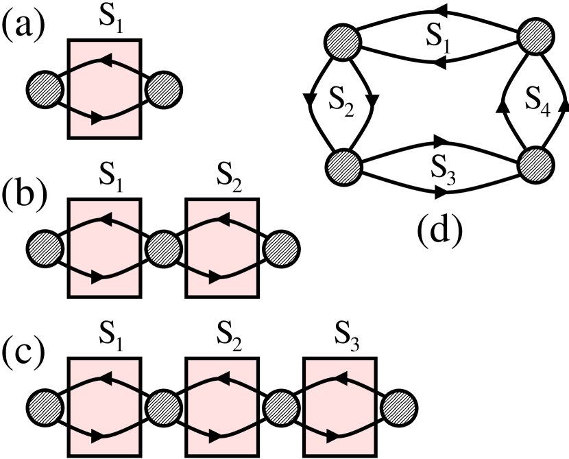
Figure 4: Structure of the diagrammatic series: The “superconducting diffusion modes” are made of pairs of nonlocal Green’s in the superconducting leads denoted by $S_{1}$, …, $S_{4}$ on the figure, which are among $\{S_{a},\,S_{b},\,S_{c,1},\,S_{c,2}\}$. The nonlocal superconducting modes connect the “nodes” corresponding to the dashed circled area. The nodes contain dressing by higher-order tunneling processes taking place locally between the 2D metal and the superconductors, and nonlocal transmission through the 2D metal. Panels a, b and c show the “diffuson-like diagrams” with superconducting diffusion modes formed of Green’s functions oriented in opposite directions. Panel c shows a “weak-localization-like diagram” with the same orientation for the pairs of nonlocal superconducting Green’s function.

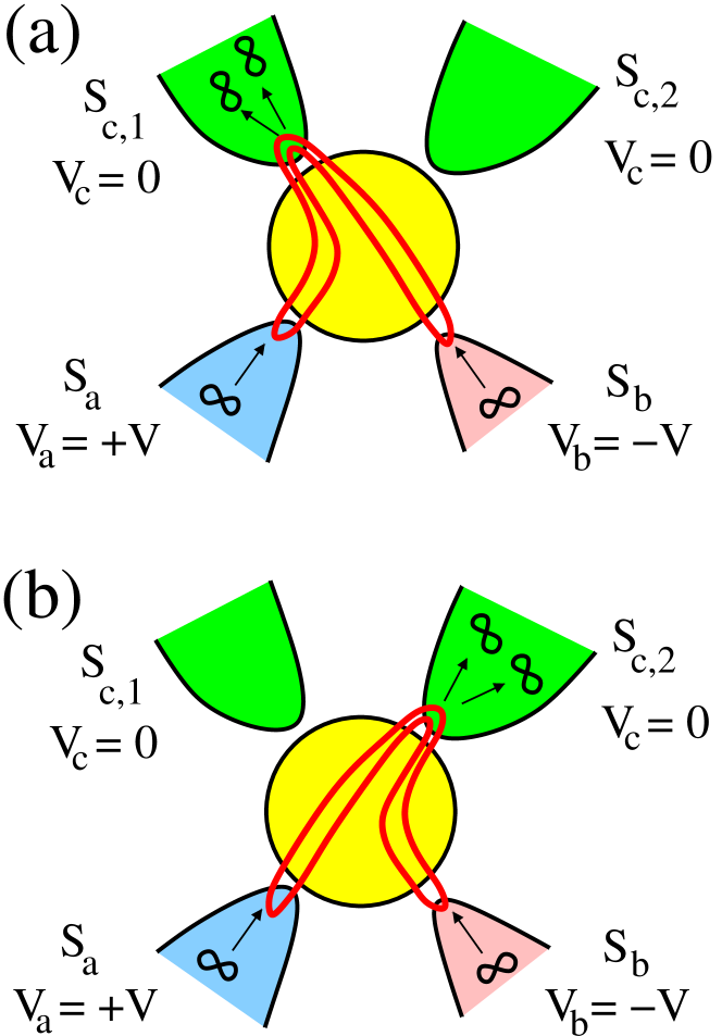
Figure 5: The lowest-order three-terminal 3TQ₁, 3TQ₂ diagrams in a real space representation (on panels a and b respectively): Two pairs are taken from $(S_{a},S_{b})$ biased at $(V,-V)$. After making a quartet from taking the square of the wave-function of a pair, the two outgoing Cooper pairs are transmitted into the grounded $S_{{c_{1}}}$ for the 3TQ₁ (panel a) or into $S_{{c_{2}}}$ for the 3TQ₂ (panel b). The 3TQ₁ and the 3TQ₂ current-phase relations are given by Eqs. (74) and (75) respectively.

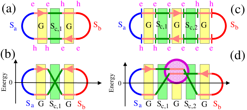
Figure 6: Diffuson and energy pictures for the three-terminal 3TQ₁ and for one of the contributions to the four-terminal 4TSQ: Panels a and b represent the three-terminal 3TQ₁ in the diffuson and in the energy pictures respectively. Panels c and d show similar representations for the four-terminal 4TSQ. The sequence of spin-up electron (e) and spin-down hole (h) Nambu labels is indicated on panels a and c. The highlighted section of the four-terminal 4TSQ diagram on panel d shows long range propagation over the mesoscopic phase coherence length $l_{\varphi}$ in between $S_{{c_{1}}}$ and $S_{{c_{2}}}$.

IV.4 Approximation on disorder for finite bias voltage and arbitrary interface transparencies

Now, we present a technical introduction to the calculations of the forthcoming section X about the interplay between disorder in the superconducting leads, arbitrary interface transparencies and finite bias voltage $V$ on the quartet line. We start with what we coin “the model I” consisting of the four-terminal device on figures 1 and 3 with superconductors in the dirty limit connected to the 2D metal by clean interfaces, see the tunnel Hamiltonian given by Eq. (13).

Within this model I, we consider expansion of the current as the closed-loop diagrams mentioned above in subsection IV.2. After forming the superconducting diffusion modes of subsection IV.3, these diagrams consist of the elements shown on figure 4:

(i) The “superconducting diffusion modes” are pairs of nonlocal superconducting Green’s functions propagating together in the superconductors over the dirty-limit coherence length given by Eq. (61).

(ii) The superconducting diffusion modes of item (i) bridge between the “nodes” shown by the dashed circles on figure 4. The nodes contain dressing by processes taking place locally between the 2D metal and the superconductors or nonlocal transmission through the 2D metal.

We consider now “the model II” as the approximation to the “model I”, see the following Hamiltonian for tunneling between the 2D metal and the superconductors within model II:

$${\cal H}_{T,\,N,\,eff}=-\sum_{\langle i,j\rangle}\sum_{\sigma=\uparrow,\downarrow}\left(J_{i\rightarrow j}c_{j,\sigma}^{+}c_{i,\sigma}+J_{j\rightarrow i}c_{i,\sigma}^{+}c_{j,\sigma}\right),$$ (64)

where the summation $\sum_{\langle i,j\rangle}$ runs over the pairs of sites on both sides of the contacts. The amplitude for hopping from $i$ (in the 2D metal layer) to $j$ (the corresponding site in the superconducting lead) is a complex number with a random phase:

$$J_{i\rightarrow j} = J_{0}\exp\left(i\psi_{i\rightarrow j}\right)$$ (65)

$$J_{j\rightarrow i} = J_{0}\exp\left(i\psi_{j\rightarrow i}\right),$$ (66)

where $\psi_{i\rightarrow j}=-\psi_{j\rightarrow i}$ and $\psi_{i\rightarrow j}$ is uniformly distributed in between $0$ and $2\pi$. The variables $\psi_{i\rightarrow j}$ and $\psi_{k\rightarrow l}$ are uncorrelated if $i,j\neq k,l$. Eqs. (65)-(66) automatically imply $\langle\langle\left(J_{i\rightarrow j}\right)^{2}\rangle\rangle=0$, which produces a vanishingly small value for the weak localization-like diagrams Melin-wl which intersect the interface with only two Green’s functions. These weak localization-like diagrams would not be washed out if disorder is introduced in the amplitudes $|J_{i\rightarrow j}|=|J_{j\rightarrow i}|$ instead of the random phases $\psi_{i\rightarrow j}=-\psi_{j\rightarrow i}$ in Eqs. (65)-(66).

However, the weak-localization-like diagrams which intersect the interfaces with four Green’s functions at the same tight-binding site are not washed out by the random $\psi_{i\rightarrow j}$ in Eqs. (65)-(66). This is because $\langle\langle|J_{i\rightarrow j}|^{4}\rangle\rangle\neq 0$ can be written as $\langle\langle\left(J_{i\rightarrow j}\right)^{2}\left(\overline{J_{i\rightarrow j}}\right)^{2}\rangle\rangle$, where the terms $\left(J_{i\rightarrow j}\right)^{2}$ and $\left(\overline{J_{i\rightarrow j}}\right)^{2}$ match both ends of a weak-localization-like loop.

Now, we provide two additional remarks:

(i) Eqs. (B.2.2)-(207) and Eqs. (208)-(214) in the dirty and ballistic limits respectively have the same dependence on energy-$\omega$, apart from different prefactors, see Appendices B and C respectively.

(ii) The opposite signs of the $\langle\langle{g_{(1,1)}g_{(1,2)}}\rangle\rangle$ modes in the dirty and ballistic limits (see subsection C.2 of Appendix C) is not relevant to the four-terminal 4TSQ, because the $\langle\langle{g_{(1,1)}g_{(1,2)}}\rangle\rangle$ modes come in pairs within each 4TSQ diagram. Their product has thus necessarily positive sign.

Based on these remarks on the structure of perturbation theory in the presence of superconductors in the dirty limit, we propose now “the model III” which is practically implemented in the forthcoming calculations of section X and includes the same weak-localization-like diagrams as model I, such as those on figure 4. The model III makes use of the nondisordered interfaces of model I combined to the ballistic limit Green’s functions of model II.

Specifically, in the model III, the interfaces are described by Eq. (13) and now, the $\{k_{F}R_{k,l}\}$ oscillations at the scale of the Fermi wave-vector are averaged out in the expression of the critical currents, where $R_{k,l}$ denotes the separation between pairs of tight-binding sites at the four interfaces within each part of the circuit, see Eqs. (19)-(22) and Eq. (25).

These arguments show that replacing model I by model III can be considered as being legitimate as a physically-motivated approximation to simulate disorder in the superconductors, i.e. to gather the superconducting Green’s functions in a pair-wise manner. The model III is used in the forthcoming section X in absence of other known method to address the interplay between disorder averaging, arbitrary interface transparencies and finite bias voltage on the quartet line, taking also the 2D metal into account. Now, we proceed with presenting our results in themselves.

V Current-phase relations of the three-terminal 3TQ and the four-terminal 4TSQ

In this section, we present a simple model for the microscopic processes contributing to the $\varphi_{q,\,3T}$-sensitive current on the quartet line. The gauge is given by Eqs. (10)-(11), and we calculate the currents in perturbation in the tunnel amplitudes and in the adiabatic limit. Subsection V.1 deals with the three-terminal quartets (3TQ₁) at the order $(J_{0}/W)^{8}$, see figure 2d. Similarly, the 3TQ₂ at the order $(J_{0}/W)^{8}$ are shown in figure 2e. Subsection V.2 describes the “four-terminal statistical fluctuations of the split quartets” (4TFSQ) at the order $(J_{0}/W)^{8}$, see figure 2f. Subsection V.3 presents the four-terminal split quartets (4TSQ) at the order $(J_{0}/W)^{12}$, see figure 2f.

We microscopically calculate the current-phase relations:

(i) Eqs. (74)-(75) for the three-terminal 3TQ₁ and the 3TQ₂.

(ii) Eq. (79) for the four-terminal 4TFSQ.

(iii) Eqs. (91)-(92) for the four-terminal 4TSQ with multichannel contacts.

These perturbative expansions nontrivially show that the three-terminal 3TQ₁, 3TQ₂ current-phase relations are $\pi$-shifted and the four-terminal 4TSQ are $0$-shifted if the contact geometry is such that $r_{0}\gg l_{e}$, where $r_{0}$ is shown on figure 3c.

V.1 The Three-Terminal quartets (3TQ₁ and 3TQ₂)

V.1.1 Microscopic calculation of the three-terminal 3TQ₁, 3TQ₂ critical currents

Now, we consider the three-terminal 3TQ₁, 3TQ₂ of Refs. Freyn, ; Melin1, (see also figure 5), and evaluate them at the order $(J_{0}/W)^{8}$ in perturbation in the tunnel amplitudes for the 2D metal which is relevant to the Harvard group experiment Harvard-group-experiment . The three-terminal 3TQ₁, 3TQ₂ transmit four fermions into the same superconducting lead, i.e. into $S_{c,\,1}$ for the 3TQ₁ (see figure 5a) or into $S_{c,\,2}$ for the 3TQ₂ (see figure 5b).

The first term $\left[\hat{J}_{a,\alpha}\hat{G}^{A}_{\alpha,a}\right]_{(1,1)}$ in the equilibrium current given by Eq. (42) takes the following form, at the lowest order $m=8$ in an expansion in $(J_{0}/W)^{m}$ and in the adiabatic limit:

$$J_{0}\langle\langle G_{[8],S_{c,1},(\alpha,a),(1,1)}^{A,(-1,-1,2,0)}\rangle\rangle = J_{0}^{8}\langle\langle g_{\alpha,\gamma_{c_{1}}}^{A,(1,1)}g_{c_{1},c_{1}}^{A,(1,2)}g_{\gamma_{c_{1}},\beta}^{A,(2,2)}g_{b,b}^{A,(2,1)}g_{\beta,\gamma_{c_{1}}}^{A,(1,1)}g_{c_{1},c_{1}}^{A,(1,2)}g_{\gamma_{c_{1}},\alpha}^{A,(2,2)}g_{a,a}^{A,(2,1)}\rangle\rangle$$ (67)

$$= J_{0}^{8}\langle\langle g_{a,a}^{A,(2,1)}\rangle\rangle\langle\langle g_{b,b}^{A,(2,1)}\rangle\rangle\langle\langle\left(g_{c_{1},c_{1}}^{A,(1,2)}\right)^{2}\rangle\rangle\langle\langle g_{\alpha,\gamma_{c_{1}}}^{A,(1,1)}g_{\gamma_{c_{1}},\alpha}^{A,(2,2)}\rangle\rangle\langle\langle g_{\beta,\gamma_{c_{1}}}^{A,(1,1)}g_{\gamma_{c_{1}},\beta}^{A,(2,2)}\rangle\rangle$$ (68)

$$= \frac{c_{1/2}}{8}\left(\frac{J_{0}}{W}\right)^{8}\frac{R_{c_{1}}}{l_{e}}\frac{1}{k_{F}R_{\alpha,\gamma_{c,1}}}\frac{1}{k_{F}R_{\beta,\gamma_{c,1}}}\frac{\Delta^{4}}{\left(\Delta^{2}-(\omega-i\eta)^{2}\right)^{2}}\exp{\left[i\left(-\varphi_{a}-\varphi_{b}+2\varphi_{c_{1}}\right)\right]},$$ (69)

where $(-1,-1,2,0)$ in the L.H.S. superscript refers to the signs in the R.H.S. $\exp\left[i\left(-\varphi_{a}-\varphi_{b}+2\varphi_{c_{1}}\right)\right]$ combination. The notation $(1,1)$ in the subscript is the same as in the preceding section IV, i.e. it stands for the “electron-electron” Nambu component.

In agreement with the diagrams on figures 6a and b, the $(1,1,-2,0)$ combination yielding $\exp\left[i\left(\varphi_{a}+\varphi_{b}-2\varphi_{c_{1}}\right)\right]$ is vanishingly small at the order $(J_{0}/W)^{8}$, if the $(1,1)$ electron-electron component is evaluated. Conversely, the $(2,2)$ hole-hole component of the $(-1,-1,2,0)$ $\exp\left[i\left(-\varphi_{a}-\varphi_{b}+2\varphi_{c_{1}}\right)\right]$ combination is vanishingly small at the order $(J_{0}/W)^{8}$.

The positive sign of Eq. (69) originates from the product of the two $\langle\langle g_{\alpha,\gamma_{c_{1}}}^{A,(1,1)}g_{\gamma_{c_{1}},\alpha}^{A,(2,2)}\rangle\rangle$ and $\langle\langle g_{\beta,\gamma_{c_{1}}}^{A,(1,1)}g_{\gamma_{c_{1}},\beta}^{A,(2,2)}\rangle\rangle$ transmission modes through the 2D metal, which both take negative values because they originate from taking the square of the pure imaginary complex number, see Eqs. (19)-(20).

The $1/8$ coefficient in Eq. (69) originates from the following terms:

(i) Each of the 2D metal transmission mode $\langle\langle g_{\alpha,\gamma_{c_{1}}}^{A,(1,1)}g_{\gamma_{c_{1}},\alpha}^{A,(2,2)}\rangle\rangle$ and $\langle\langle g_{\beta,\gamma_{c_{1}}}^{A,(1,1)}g_{\gamma_{c_{1}},\beta}^{A,(2,2)}\rangle\rangle$ yields a $\langle\langle\cos^{2}(k_{F}R)\rangle\rangle=1/2$ factor, see Eqs. (19)-(20).

(ii) A $1/2$ coefficient is related by convention to the superconducting diffusion mode $\langle\langle\left(g_{c_{1},c_{1}}^{A,(1,2)}\right)^{2}\rangle\rangle$ which is taken to be dominated by nonlocal propagation over the dirty-limit coherence length on the $S_{c,1}$ side of the 2D metal-$S_{c,1}$ interface.

Integrating the spectral current given by Eq. (69) over energy $\omega$ produces a positive sign because the residue at $\omega=-\Delta$ is positive, see Eqs. (229)-(230) in Appendix D.1. In the limit of zero temperature, the above Eqs. (67)-(69) and Eqs. (229)-(231) in Appendix D.1 lead to

$$\int_{-\infty}^{0}J_{0}\langle\langle G_{[8],S_{c,1},(\alpha,a),(1,1)}^{A,(-1,-1,2,0)}\rangle\rangle(\omega)d\omega = \frac{i\pi c^{\prime}_{1/2}\Delta}{32}\left(\frac{J_{0}}{W}\right)^{8}\frac{\sqrt{{\cal S}_{contact}}}{l_{e}}\frac{y_{0}z_{0}}{(k_{F}R_{0})^{2}}\exp{\left[i\left(-\varphi_{a}-\varphi_{b}+2\varphi_{c_{1}}\right)\right]}.$$ (70)

Evaluating similarly all terms in Eqs. (42)-(45) leads to

$$I_{\alpha\rightarrow a,eq}=I_{c,\,3TQ_{1}}\sin\varphi_{q,\,3T,\,1},$$ (71)

where

$$\varphi_{q,\,3T,\,1}=\varphi_{a}+\varphi_{b}-2\varphi_{c_{1}}.$$ (72)

The SQ₁ critical current $I_{c,\,3TQ_{1}}$ is negative, i.e. it is $\pi$-shifted:

$$I_{c,\,3TQ_{1}}=-\frac{ec^{\prime}_{1/2}\pi\Delta}{4\hbar}\left(\frac{J_{0}}{W}\right)^{8}\frac{\sqrt{{\cal S}_{contact}}}{l_{e}}\frac{y_{0}z_{0}}{(k_{F}R_{0})^{2}}.$$ (73)

Finally, we define the remaining variables appearing in Eqs. (69)-(73).

The coefficients $c_{1/2}$ and $c^{\prime}_{1/2}$ are positive and of order unity.

The dimensionless parameters $y_{0}$ and $z_{0}$ in Eqs. (70)-(73) depend on the shape of the four-terminal device, still within the short junction limit assumption, see subsection III.1.1 for a discussion of the short-junction limit and figure 3 for the definition of $y_{0}$ and $z_{0}$.

The $1/k_{F}R_{\alpha,\gamma_{c,1}}$ and $1/k_{F}R_{\beta,\gamma_{c,1}}$ terms in Eq. (69) originate from ballistic propagation through the 2D metal, see Eqs. (19)-(22).

In connection with subsection IV.3, we assumed small area ${\cal S}_{contact}=\pi R_{c,1}^{2}$ for the circular contact between the 2D metal and the superconducting lead $S_{c,1}$, such that $R_{c,1}\lesssim\xi_{dirty}(0)$, where the dirty-limit coherence length is given by Eq. (61) and the geometry is shown schematically on figure 3c. The assumption $R_{c,1}\lesssim\xi_{dirty}(0)$ yields the $R_{c,1}/l_{e}\sim\sqrt{{\cal S}_{contact}}/l_{e}$ scaling in Eq. (69), (70) and Eq. (73), see also the discussion in the preceding subsection IV.3.

V.1.2 Discussion

The following current-phase-flux relations are deduced from Eq. (71) in the gauge given by Eqs. (10)-(11):

$$I_{3TQ_{1}}(\varphi_{q,\,3T},\Phi) = I_{c,\,3TQ_{1}}\sin\left[\varphi_{q,\,3T}+\Phi\right]$$ (74)

$$I_{3TQ_{2}}(\varphi_{q,\,3T},\Phi) = I_{c,\,3TQ_{2}}\sin\left[\varphi_{q,\,3T}-\Phi\right],$$ (75)

where Eq. (74) and Eq. (75) correspond to the three-terminal 3TQ₁, 3TQ₂ respectively. The phase variable entering Eq. (74) is $\varphi_{q,\,3T,\,1}\equiv\varphi_{a}+\varphi_{b}-2\varphi_{{c_{1}}}\equiv\varphi_{q,\,3T}+\Phi$ and that entering Eq. (75) is $\varphi_{q,\,3T,\,1}\equiv\varphi_{a}+\varphi_{b}-2\varphi_{{c_{2}}}\equiv\varphi_{q,\,3T}-\Phi$, where $\varphi_{{c_{1}}}$ and $\varphi_{{c_{2}}}$ are given by Eqs. (10)-(11), and $\varphi_{q,\,3T}$ is given by Eq. (6).

Figures 6a and b show two representations of the three-terminal 3TQ₁:

(i) Figure 6a shows a representation resembling the “diffusons” in the theory of disordered conductors.

(ii) Figure 6b shows energy on the $y$-axis, with respect to the chemical potential of the grounded $S_{c}$, see also Ref. Freyn, ; Melin1, .

In addition, an intuitive argument for the $\pi$-shift in the three-terminal 3TQ₁, 3TQ₂ current-phase relations Eqs. (71)-(75) is the following Jonckheere :

The two Cooper pairs of the quartets imply taking the square of the single-pair wave-function

$$\frac{1}{\sqrt{2}}\left(c_{a,\uparrow}^{+}c_{b,\downarrow}^{+}-c_{a,\downarrow}^{+}c_{b,\uparrow}^{+}\right)$$ (76)

according to

$$\frac{1}{2}\left(c_{a,\uparrow}^{+}c_{b,\downarrow}^{+}-c_{a,\downarrow}^{+}c_{b,\uparrow}^{+}\right)^{2}.$$ (77)

Eq. (77) takes the form of the opposite of a pair of pair:

$$\mbox{(\ref{eq:square})}=-\left(c_{a,\uparrow}^{+}c_{a,\downarrow}^{+}\right)\left(c_{b,\uparrow}^{+}c_{b,\downarrow}^{+}\right).$$ (78)

The minus sign appearing in the R.H.S. of Eq. (78) is consistent with the $\pi$-shifted critical current in Eq. (73), which receives interpretation of macroscopic manifestation for the internal structure of a Cooper pair, i.e. the orbital and spin symmetries.

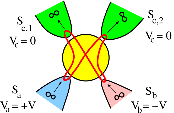
Figure 7: The diagram encoding the four-terminal statistical fluctuations of the split quartets (4TFSQ) transmits one Cooper pair into $S_{{c_{1}}}$ and another one into $S_{{c_{2}}}$. The four-terminal 4TFSQ diagrams encode a statistical fluctuation of the $\varphi_{q,\,3T}$-sensitive current which does not scale with the number of channels. (This is because the Green’s functions cannot be gathered in a pair-wise manner on this diagram). The four-terminal 4TFSQ current-phase relation is given by Eq. (79).

V.2 The Four-Terminal statistical Fluctuations of the Split Quartet current (4TFSQ)

Before discussing in the next subsection V.3 the four-terminal 4TSQ at the order $(J_{0}/W)^{12}$, we mention now a simpler “baby-4TSQ” at the order $(J_{0}/W)^{8}$ , see figure 7. The critical current of this order-$(J_{0}/W)^{8}$ process is small, and it fluctuates around zero value. The reason is that the four single-particle Green’s functions crossing the 2D metal on figure 7 cannot be gathered in a pair-wise manner if the four contacts with the superconducting leads $S_{a}$, $S_{b}$, $S_{c,1}$ and $S_{c,2}$ make between them distance which is much larger than the Fermi wave-length $\lambda_{F}$. The current associated to the four-terminal 4TFSQ of order $(J_{0}/W)^{8}$ on figure 7 is given by

$$I_{4TFSQ}(\varphi_{q,\,3T}) = I_{c,\,4TFSQ}\sin\varphi_{q,\,4T},$$ (79)

where

$$\varphi_{q,\,4T}=\varphi_{a}+\varphi_{q,\,3T}-\varphi_{c,1}-\varphi_{c,2}.$$ (80)

Eqs. (10)-(11) imply $\varphi_{q,\,4T}=\varphi_{q,\,3T}$, where $\varphi_{q,\,3T}$ is given by Eq. (6). Overall, multichannel averaging produces a vanishingly small critical current for the four-terminal 4TFSQ: $\langle\langle I_{c,\,4TFSQ}\rangle\rangle=0$.

V.3 The Four-Terminal Split Quartets (4TSQ)

Now, we consider the four-terminal 4TSQ yielding nonvanishingly small value for critical current with multichannel interfaces. Two types of diagrams appear at the order $(J_{0}/W)^{12}$, after a first selection has been operated with respect to gathering the nonlocal Green’s functions through the 2D metal in a pair-wise manner:

(i) The diagrams containing products of three Nambu Green’s functions within the same superconducting lead: Their critical current is of order $\sqrt{{\cal S}_{contact}}/l_{e}$, see the forthcoming subsection V.3.1 and subsection II A in the Supplemental Materialsupplemental .

(ii) The remaining diagrams provide the leading-order ${\cal S}_{contact}/l_{e}^{2}$ contribution to the critical current, see the forthcoming subsection V.3.2 and subsection II B in the Supplemental Materialsupplemental .

V.3.1 The four-terminal 4TSQ current at the orders $(J_{0}/W)^{12}$ and $\sqrt{{\cal S}_{contact}}/l_{e}$

We provide now the microscopic calculation for the contributions to $J_{a,\alpha}G^{A}_{\alpha,a}$ at the orders $(J_{0}/W)^{12}$ and $\sqrt{{\cal S}_{contact}}/l_{e}$. The four terms given below in Eqs. (81)-(84) correspond to the following possibilities:

(i) The $(1,1)$ “electron-electron” or the $(2,2)$ “hole-hole” components of $J_{a,\alpha}G^{A}_{\alpha,a}$.

(ii) The $\exp\left[\pm i\left(+\varphi_{a}+\varphi_{b}-\varphi_{c,1}-\varphi_{c,2}\right)\right]$ factors for the $(1,1,-1,-1)$ or $(-1,-1,1,1)$ labels respectively.

We obtain the following:

$$J_{0}\langle\langle G_{[12],(\alpha,a),(1,1),(1)}^{A,(1,1,-1,-1)}\rangle\rangle_{total}(\omega) = \frac{c^{\prime}_{1/2}}{8}\left(\frac{J_{0}}{W}\right)^{12}\frac{\sqrt{{\cal S}_{contact}}}{l_{e}}\frac{x_{0}y_{0}z_{0}}{(k_{F}R_{0})^{3}}\frac{\Delta^{6}}{\left(\Delta^{2}-(\omega-i\eta)^{2}\right)^{3}}\exp{\left[i\left(\varphi_{a}+\varphi_{b}-\varphi_{c_{1}}-\varphi_{c_{2}}\right)\right]}$$ (81)

$$J_{0}\langle\langle G_{[12],(\alpha,a),(1,1),(1)}^{A,(-1,-1,1,1)}\rangle\rangle_{total}(\omega) = \frac{5c^{\prime}_{1/2}}{8}\left(\frac{J_{0}}{W}\right)^{12}\frac{\sqrt{{\cal S}_{contact}}}{l_{e}}\frac{x_{0}y_{0}z_{0}}{(k_{F}R_{0})^{3}}\frac{\Delta^{6}}{\left(\Delta^{2}-(\omega-i\eta)^{2}\right)^{3}}\exp{\left[i\left(-\varphi_{a}-\varphi_{b}+\varphi_{c_{1}}+\varphi_{c_{2}}\right)\right]}$$ (82)

$$J_{0}\langle\langle G_{[12],(\alpha,a),(2,2),(1)}^{A,(1,1,-1,-1)}\rangle\rangle_{total}(\omega) = \frac{5c^{\prime}_{1/2}}{8}\left(\frac{J_{0}}{W}\right)^{12}\frac{\sqrt{{\cal S}_{contact}}}{l_{e}}\frac{x_{0}y_{0}z_{0}}{(k_{F}R_{0})^{3}}\frac{\Delta^{6}}{\left(\Delta^{2}-(\omega-i\eta)^{2}\right)^{3}}\exp{\left[i\left(\varphi_{a}+\varphi_{b}-\varphi_{c_{1}}-\varphi_{c_{2}}\right)\right]}$$ (83)

$$J_{0}\langle\langle G_{[12],(\alpha,a),(2,2),(1)}^{A,(-1,-1,1,1)}\rangle\rangle_{total}(\omega) = \frac{c^{\prime}_{1/2}}{8}\left(\frac{J_{0}}{W}\right)^{12}\frac{\sqrt{{\cal S}_{contact}}}{l_{e}}\frac{x_{0}y_{0}z_{0}}{(k_{F}R_{0})^{3}}\frac{\Delta^{6}}{\left(\Delta^{2}-(\omega-i\eta)^{2}\right)^{3}}\exp{\left[i\left(-\varphi_{a}-\varphi_{b}+\varphi_{c_{1}}+\varphi_{c_{2}}\right)\right]}.$$ (84)

The microscopic process contributing to the $(-1,-1,1,1)$ terms given by Eq. (82) and Eq. (84) are listed in subsection II A of the Supplemental Materialsupplemental . Specifically, Eq. (82) is the sum of Eqs. (10)-(39) in the Supplemental Materialsupplemental and Eq. (84) is the sum of Eqs. (41)-(46), also in the Supplemental Materialsupplemental .

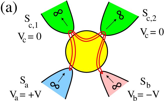
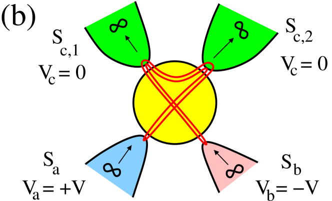
Figure 8: Two of the Four-Terminal Split Quartet diagrams (4TSQ): Contrary to the previous four-terminal 4TFSQ diagram (see figure 7), these four-terminal 4TSQ diagrams yield a critical current which is not a small statistical fluctuation. On the contrary, the four-terminal 4TSQ current scales with the number of channels because the Green’s functions are gathered in a pair-wise manner on this figure.

The overall positive sign of Eqs. (81)-(84) originates from the product of four negative contributions:

(i) A minus sign is associated to each of the three transmission modes through the 2D metal.

(ii) Another minus sign is due to averaging the product of three superconducting Green’s functions, see Eqs. (237)-(241) in Appendix D.4.

In addition, the $\exp{\left[i\left(-\varphi_{a}-\varphi_{b}+\varphi_{c_{1}}+\varphi_{c_{2}}\right)\right]}$ factor in Eqs. (82) and (84) produces a “(1,1)” electron-electron Nambu component $5/8$ coefficient in Eq. (82) which is larger than the “$(2,2)$” hole-hole component $1/8$ coefficient in Eq. (84). This is compatible with the observation that the “$(2,2)$” component associated with the $(-1,-1,2,0)$ combination is vanishingly small for the three-terminal 3TQ₁, see the above subsection V.1.

In addition, the residue of the pole at $\omega=-\Delta$ is positive, see Eqs. (232)-(234) in Appendix D.2 concerning the integral over the energy $\omega$.

Overall, Eqs. (40)-(40) and Eqs. (81)-(84) lead to the following current-phase relation for the 4TSQ at the orders $(J_{0}/W)^{12}$ and $\sqrt{{\cal S}_{contact}}/l_{e}$:

$$I_{\alpha\rightarrow a,eq}^{(1)}=I_{c,\,4TSQ}^{(1)}\sin\varphi_{q,\,4T},$$ (85)

where $\varphi_{q,\,4T}\equiv\varphi_{a}+\varphi_{b}-\varphi_{c,1}-\varphi_{c,2}\equiv\varphi_{q,\,3T}$, as for the 4TFSQ, see Eqs. (79)-(80).

The critical current $I_{c,\,4TSQ}^{(1)}$ appearing in Eq. (85) is negative, i.e. it is $\pi$-shifted:

$$I_{c,\,4TSQ}^{(1)}=-\frac{3ec^{\prime}_{1/2}\pi\Delta}{4\hbar}\left(\frac{J_{0}}{W}\right)^{12}\frac{\sqrt{{\cal S}_{contact}}}{l_{e}}\frac{x_{0}y_{0}z_{0}}{(k_{F}R_{0})^{3}}.$$ (86)

V.3.2 The four-terminal 4TSQ current at the orders $(J_{0}/W)^{12}$ and ${\cal S}_{contact}/l_{e}^{2}$

Next, we calculate the four-terminal 4TSQ critical current at the orders $(J_{0}/W)^{12}$ and ${\cal S}_{contact}/l_{e}^{2}$. Again, we separate between the “electron-electron” from the “hole-hole” Nambu components, and the $\exp\left[\pm i\left(+\varphi_{a}+\varphi_{b}-\varphi_{c,1}-\varphi_{c,2}\right)\right]$ sensitivity on the superconducting phase variables:

$$J_{0}\langle\langle G_{[12],(\alpha,a),(1,1),(2)}^{A,(1,1,-1,-1)}\rangle\rangle_{total}(\omega) = -\frac{c^{\prime}_{1}}{32}\left(\frac{J_{0}}{W}\right)^{12}\frac{{\cal S}_{contact}}{l_{e}^{2}}\frac{y_{0}z_{0}^{2}+y_{0}^{2}z_{0}+x_{0}z_{0}^{2}+x_{0}y_{0}^{2}}{(k_{F}R_{0})^{3}}\frac{(\omega-i\eta)^{2}\Delta^{4}}{\left(\Delta^{2}-(\omega-i\eta)^{2}\right)^{3}}e^{i\left(\varphi_{a}+\varphi_{b}-\varphi_{c_{1}}-\varphi_{c_{2}}\right)}$$ (87)

$$J_{0}\langle\langle G_{[12],(\alpha,a),(1,1),(2)}^{A,(-1,-1,1,1)}\rangle\rangle_{total}(\omega) = -\frac{5c^{\prime}_{1}}{32}\left(\frac{J_{0}}{W}\right)^{12}\frac{{\cal S}_{contact}}{l_{e}^{2}}\frac{y_{0}z_{0}^{2}+y_{0}^{2}z_{0}+x_{0}z_{0}^{2}+x_{0}y_{0}^{2}}{(k_{F}R_{0})^{3}}\frac{(\omega-i\eta)^{2}\Delta^{4}}{\left(\Delta^{2}-(\omega-i\eta)^{2}\right)^{3}}e^{i\left(-\varphi_{a}-\varphi_{b}+\varphi_{c_{1}}+\varphi_{c_{2}}\right)}$$ (88)

$$J_{0}\langle\langle G_{[12],(\alpha,a),(2,2),(2)}^{A,(1,1,-1,-1)}\rangle\rangle_{total}(\omega) = -\frac{5c^{\prime}_{1}}{32}\left(\frac{J_{0}}{W}\right)^{12}\frac{{\cal S}_{contact}}{l_{e}^{2}}\frac{y_{0}z_{0}^{2}+y_{0}^{2}z_{0}+x_{0}z_{0}^{2}+x_{0}y_{0}^{2}}{(k_{F}R_{0})^{3}}\frac{(\omega-i\eta)^{2}\Delta^{4}}{\left(\Delta^{2}-(\omega-i\eta)^{2}\right)^{3}}e^{i\left(\varphi_{a}+\varphi_{b}-\varphi_{c_{1}}-\varphi_{c_{2}}\right)}$$ (89)

$$J_{0}\langle\langle G_{[12],(\alpha,a),(2,2),(2)}^{A,(-1,-1,1,1)}\rangle\rangle_{total}(\omega) = -\frac{c^{\prime}_{1}}{32}\left(\frac{J_{0}}{W}\right)^{12}\frac{{\cal S}_{contact}}{l_{e}^{2}}\frac{y_{0}z_{0}^{2}+y_{0}^{2}z_{0}+x_{0}z_{0}^{2}+x_{0}y_{0}^{2}}{(k_{F}R_{0})^{3}}\frac{(\omega-i\eta)^{2}\Delta^{4}}{\left(\Delta^{2}-(\omega-i\eta)^{2}\right)^{3}}e^{i\left(-\varphi_{a}-\varphi_{b}+\varphi_{c_{1}}+\varphi_{c_{2}}\right)}$$ (90)

Eq. (88) is the sum of Eqs. (48)-(107) in subsection II B of the Supplemental Materialsupplemental . Eq. (90) is the sum of Eqs. (109)-(120) in the Supplemental Materialsupplemental .

The minus sign in Eqs. (87)-(90) is due to the product of three (negative) transmission modes through the 2D metal.

In addition, the $\exp{\left[i\left(-\varphi_{a}-\varphi_{b}+\varphi_{c_{1}}+\varphi_{c_{2}}\right)\right]}$ combination yields the $5/32$ coefficient for the “$(1,1)$” component which is larger than $1/32$ for the “$(2,2)$” component, see Eqs. (88) and (90) respectively. This is compatible with the discussion following the above Eqs. (81)-(84).

A (positive) residue is taken into account in the integral over energy, see Eqs. (235)-(236) in Appendix D.3.

It is deduced that Eqs. (42)-(45) and Eqs. (87)-(90) lead to the following contribution to the equilibrium current $I_{\alpha\rightarrow a,eq}$ at the orders $(J_{0}/W)^{12}$ and ${\cal S}_{contact}/l_{e}^{2}$:

$$I_{\alpha\rightarrow a,eq}^{(2)}=I_{c,\,4TSQ}^{(2)}\sin\varphi_{q,\,4T},$$ (91)

where $\varphi_{q,\,4T}$ is given by Eq. (80) and the critical current $I_{c,\,4TSQ}^{(2)}$ is positive, i.e. it is $0$-shifted:

$$I_{c,\,4TSQ}^{(2)}=\frac{3ec^{\prime}_{1}\Delta}{16\hbar}\left(\frac{J_{0}}{W}\right)^{12}\frac{{\cal S}_{contact}}{l_{e}^{2}}\frac{y_{0}z_{0}^{2}+y_{0}^{2}z_{0}+x_{0}z_{0}^{2}+x_{0}y_{0}^{2}}{(k_{F}R_{0})^{3}}.$$ (92)

V.3.3 Discussion

Two of the four-terminal 4TSQ diagrams appearing at the orders $(J_{0}/W)^{12}$ and ${\cal S}_{contact}/l_{e}^{2}$ are shown on figures 8a and b. The diffuson and the energy representations on figures 6c, d respectively illustrate that the four-terminal 4TSQ of orders $(J_{0}/W)^{12}$ and ${\cal S}_{contact}/l_{e}^{2}$ involve the product of two superconducting diffusion modes of the $\langle\langle{g_{(1,1)}g_{(1,2)}}\rangle\rangle$-type. For instance, the superconducting diffusion modes propagating in $S_{c,1}$ or in $S_{c,2}$ on figures 8a and b correspond to the $x_{0}y_{0}^{2}$ or $x_{0}z_{0}^{2}$ contributions to Eqs. (87)-(90) respectively [see also Eq. (92)].

The $0$-shifted four-terminal 4TSQ current [see Eqs. (91)-(92)] is interpreted as the intermediate state

$$c_{S_{c_{1}},\uparrow}^{+}c_{S_{c_{1}},\downarrow}^{+}c_{S_{c_{2}},\uparrow}^{+}c_{S_{c_{2}},\downarrow}^{+}$$ (93)

made with two Cooper pairs from $S_{a}$ and $S_{b}$ biased at $\pm V$. Anticommuting the $(S_{{c_{1}}},\uparrow)$ and the $(S_{{c_{2}}},\uparrow)$ partners in Eq. (93) leads to a minus sign which implies $0$-shift for the four-terminal 4TSQ current-phase relation [see Eqs. (91)-(92)) in comparison with the previous $\pi$-shift of the three-terminal 3TQ₁ and 3TQ₂ [see Eqs. (71)-(73)]. Indeed, the three-terminal 3TQ₁ and 3TQ₂ do not contain the additional two-fermion exchange of the 4TSQ which is made possible by the 2D quantum wake, see the forthcoming section VII.

VI Interference between the three-terminal 3TQ₁, 3TQ₂ and the four-terminal 4TSQ

We proceed by further considering that, in the gauge given by Eqs. (10)-(11), the $\varphi_{q,\,3T}$-sensitive critical current is the result of an interference between the three-terminal 3TQ₁, 3TQ₂ (see subsection V.1), and the four-terminal 4TSQ (see subsection V.3):

$$I_{c}(\Phi/\Phi_{0}) = \mbox{Max}_{\varphi_{q,\,3T}}\left[I_{3TQ_{1}}(\varphi_{q,\,3T},\Phi)\right.$$

$$\left.+I_{3TQ_{2}}(\varphi_{q,\,3T},\Phi)+I_{4TSQ}(\varphi_{q,\,3T})\right].$$

The contact areas ${\cal S}_{contact}$ are considered to be large compared to $(l_{e})^{2}$, i.e. ${\cal S}_{contact}\gg l_{e}^{2}$. This realistic assumption yields $|I_{c,\,4TSQ}^{(1)}|\ll I_{c,\,4TSQ}^{(2)}$. The four-terminal 4TSQ critical current is approximated as $I_{4TSQ}(\varphi_{q,\,3T})\simeq I_{c,\,4TSQ}^{(2)}$. The resulting current-phase relation

$$I_{4TSQ}(\varphi_{q,\,3T})\simeq I_{c,\,4TSQ}^{(2)}\sin\varphi_{q,\,3T}$$ (95)

is independent on the value of the magnetic flux $\Phi$, see the expression of $\varphi_{q,\,3T}$ given by Eq. (6) and $I_{c,\,4TSQ}^{(2))}$ in Eq. (92).

Eq. (VI) is $2\pi$-periodic in $\Phi$, while the previous $\mbox{Max}_{\varphi_{q,\,3T}}\left[I_{3TQ_{1}}(\varphi_{q,\,3T},\Phi)+I_{3TQ_{2}}(\varphi_{q,\,3T},\Phi)\right]$ was $\pi$-periodic.

More specifically, specializing to $\Phi/\Phi_{0}=0$ and to $\Phi/\Phi_{0}=1/2$ leads to

$$I_{c}(0)=\left|I_{c,\,3TQ_{1}}+I_{c,\,3TQ_{2}}+I_{c,\,4TSQ}\right|,$$ (96)

which is different from

$$I_{c}(1/2)=\left|I_{c,\,3TQ_{1}}+I_{c,\,3TQ_{2}}-I_{c,\,4TSQ}\right|.$$ (97)

VII Why the four-terminal 4TSQ appear only in 2D

The preceding section V presented the calculation (in perturbation in $J_{0}/W$ and in the adiabatic limit $V=0^{+}$) of the sign and the amplitude of the $\pi$-shifted three-terminal 3TQ₁, 3TQ₂ and the $0$-shifted four-terminal 4TSQ critical currents. We proceed further with discussing why the four-terminal 4TSQ yields a vanishingly small current if a 1D or 3D metal is used instead of the 2D metal such as graphene gated away from the Dirac point in the Harvard group experiment Harvard-group-experiment .

We establish a link between Eqs. (19)-(22) for the Green’s function of a ballistic 2D metal, and the general theory of the “wake” in the solution of the even-dimensional wave-equation, starting in subsection VII.1 with the classical wave equation. The 2D quantum wake in nanoscale electronic devices is considered in subsection VII.2. Synchronizing two Josephson junctions with quasiparticles “surfing” on the 2D quantum wake is discussed in subsection VII.3, in connection with the features of the four-terminal 4TSQ diagram, see one of the 4TSQ diagrams in figure 6d. A summary of this section VII is presented in subsection VII.4.

At this point, we also make reference to a very recent preprintquantum-wakes-cold-atoms about the production of quantum wakes with ultracold atoms.

VII.1 The wake effect in the classical wave equation

Volterra was the first to understand that the solutions of the wave-equation are drastically different in even or odd space dimension. Let us assume that an excitation is produced at given location and time. A detector is at distance $R$ from the location of the excitation. In all cases, the signal reaches $R$ after the time delay $t_{0}=R/v$, where $v$ is the speed of wave propagation. In odd dimensions (such as in 1D or 3D), the detected signal consists of the sharp pulse associated the wave-front. But in even dimension (such as in 2D), the detected signal oscillates long after the time delay $t_{0}$. This “classical wake” appears in even space dimensions but not in odd dimensions, and it meets common sense regarding a boat propagating on a calm sea.

VII.2 The 2D quantum wake in meso or nanoscale devices

The signal at the detector mentioned above results from a convolution of the initial excitation with the $D$-dimensional Green’s functions. It turns out that Green’s functions are at the heart of the calculation of the electronic transport properties in meso or nanoscale devices.

The normal-state Green’s function at distance $R$ is a plane-wave in 1D:

$$g^{A}_{1D,\,(1,1)}(R,\omega)\sim\exp(ikR),$$ (98)

where $k$ is the wave-vector at the considered energy $\omega$ and “$(1,1)$” refers to the “spin-up electron” Nambu component. The 3D Green’s function is also a plane wave:

$$g^{A}_{3D,\,(1,1)}(R,\omega)\sim\frac{\exp(ikR)}{kR},$$ (99)

which is normalized by the factor $kR$ arising from probability conservation. In 2D, the Green’s function is a Bessel function which behaves like

$$g^{A}_{2D,\,(1,1)}(R,\omega)\sim i\frac{\cos(kR-\pi/4)}{\sqrt{kR}}$$ (100)

at large $R\gg 1/k$, see the above Eq. (19) and Appendix A for the demonstration of Eqs. (19) and (100).

VII.3 Synchronizing two Josephson junctions by the 2D quantum wake

The difference between the 1D or 3D $\exp(ikR)$ oscillations in Eqs. (98) and (99), and the 2D $\cos(kR-\pi/4)$ oscillations in Eq. (100) is now discussed in connection with synchronizing two Josephson junctions.

Specifically, we focus on the highlighted section of the four-terminal 4TSQ diagram on figure 6d, which involves taking the square of the advanced Green’s function according to $\left[g^{A}_{(1,1)}(R)\right]^{2}$. Multichannel interfaces are simulated by averaging $\left[g^{A}_{(1,1)}(R)\right]^{2}$ over $R$ around the value $R_{0}$ such that $\lambda_{F}\ll R_{0}\lesssim l_{\varphi}$. Averaging over the separation $R$ between $S_{c,1}$ and $S_{c,2}$ in an interval of width $\Delta R\sim 2\pi/k$ around $R=R_{0}$ yields

$$\langle\langle\left[g^{A}_{1D,\,(1,1)}(R)\right]^{2}\rangle\rangle = 0$$ (101)

$$\langle\langle\left[g^{A}_{2D,\,(1,1)}(R)\right]^{2}\rangle\rangle \simeq -\frac{1}{2W^{2}k_{F}R_{0}}$$ (102)

$$\langle\langle\left[g^{A}_{3D,\,(1,1)}(R)\right]^{2}\rangle\rangle = 0.$$ (103)

Eqs. (101)-(103) are deduced from Eqs. (98), (19) and (99) respectively. These Eqs. (101)-(103) imply short range coupling over $\lambda_{F}$ if a 1D or a 3D metal is used instead of a 3D metal, which is in agreement with the general theory of the 2D wake mentioned above.

To summarize, it is only in 2D that the 4TSQ diagrams on figures 6c and d are nonvanishingly small, due to the nonvanishingly small $\langle\langle\left[g^{A}_{(1,1)}(R)\right]^{2}\rangle\rangle\neq 0$ connecting $S_{{c_{1}}}$ and $S_{{c_{2}}}$ on figure 6d, and physically encoding the exchange of a quasiparticle via the 2D quantum wake.

VII.4 Summary of this section

The microscopic theory of the four-terminal 4TSQ was discussed:

(i) The four-terminal 4TSQ are specific to 2D, and they are related to the quantum limit of the wake in the even-dimensional wave-equation.

(ii) The four-terminal 4TSQ realize quantum mechanical synchronization between Josephson junctions by coherently exchanging a quasiparticle between them. The quasiparticle which is exchanged propagates on the 2D quantum wake.

(iii) The four-terminal 4TSQ couple the Andreev bound states of the two Josephson junctions in the simple limit of equilibrium with bias voltage $V=0$, and in the adiabatic limit with $V=0^{+}$ on the quartet line, see also the remarks on the long range coupling of the four-terminal 4TSQ in the concluding subsection XI.3.

Finally, we note that the four-terminal 4TSQ do not contribute to the current in the previous Grenoble group experiment Lefloch . In this experiment, the intermediate region connecting the superconducting leads consists of an evaporated “T-shaped” Copper lead which is 3D, as opposed to the atomically thin 2D sheet of graphene used in the Harvard group experiment Harvard-group-experiment . The 2D quantum wake is neither expected to play a role in the Weizmann Institute group experiment Heiblum made with a semiconducting nanowire.

VIII Inversion between $\Phi/\Phi_{0}=0$ and $\Phi/\Phi_{0}=1/2$

In this section, we show that the relative shift of $\pi$ between the three-terminal 3TQ₁, 3TQ₂ and the four-terminal 4TSQ obtained in the above section V, implies emergence of the inversion $I_{c}(0)<I_{c}(1/2)$ between $\Phi/\Phi_{0}=0$ and $\Phi/\Phi_{0}=1/2$ in the reduced flux $\Phi/\Phi_{0}$ dependence of the critical current $I_{c}(\Phi/\Phi_{0})$ given by Eqs. (VI)-(95).

In addition, we address the reverse question of the information which is deduced from “Observation of inversion in $I_{c}(\Phi/\Phi_{0})$ between $\Phi/\Phi_{0}=0$ and $\Phi/\Phi_{0}=1/2$”, regarding the sign of the three-terminal 3TQ₁, 3TQ₂ and the four-terminal 4TSQ current-phase relations.

The assumptions about the $0$- and $\pi$- shifted current-phase relations are presented in subsection VIII.1. The reasoning in itself is presented in subsection VIII.2. The consequences for the Harvard group experiment are provided in subsection VIII.3.

VIII.1 The assumptions

This subsection is based on the following assumptions:

(i) We have information about the $\Phi/\Phi_{0}$-sensitivity of the critical current $I_{c}$, more specifically about whether $I_{c}(0)$ is smaller or larger than $I_{c}(1/2)$.

(ii) The signs of the three-terminal 3TQ₁, 3TQ₂ and the four-terminal 4TSQ critical currents are left a free parameters, while they interfere according to the preceding Eq. (VI).

VIII.2 General statements

Let us now assume that inversion $I_{c}(0)<I_{c}(1/2)$ between $\Phi/\Phi_{0}=0$ and $\Phi/\Phi_{0}=1/2$ is observed. Combining Eqs. (96), (97) to Eq. (121) in section III of the Supplemental Material supplemental yields the following “logical chain”:

$$I_{c}(0)<I_{c}(1/2)$$ (104)

$$\iff \left|I_{c,\,3TQ_{1}}+I_{c,\,3TQ_{2}}+I_{c,\,4TSQ}\right|$$

$$<\left|I_{c,\,3TQ_{1}}+I_{c,\,3TQ_{2}}-I_{c,\,4TSQ}\right|$$

$$\iff I_{c,\,3TQ_{1}}+I_{c,\,3TQ_{2}}\mbox{ and }I_{c,\,4TSQ}$$

have opposite signs.

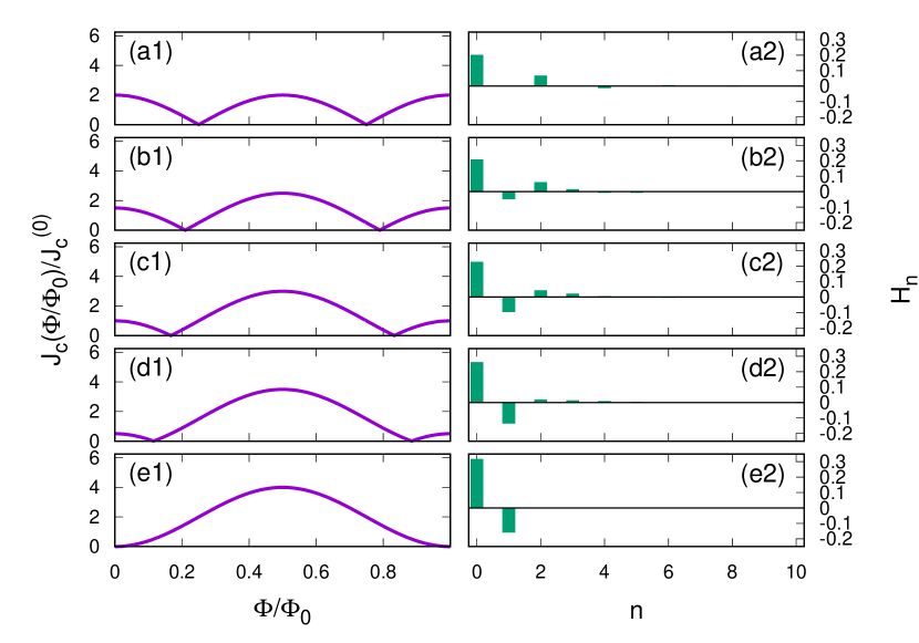
Figure 9: Critical current-flux relations (panel a1-e1) and the corresponding Fourier coefficients (panels a2-e2): The parameters $\alpha_{3TQ_{1}}=\alpha_{3TQ_{2}}=-1$ are used, and $\alpha_{4TSQ}=0,\,0.5,\,1,\,\,1.5,\,2$ on panels a1-a2, b1-b2, c1-c2, d1-d2 and e1-e2 respectively. The opposite signs of $\alpha_{3TQ_{1}}<0$, $\alpha_{3TQ_{2}}<0$ and $\alpha_{4TSQ}\geq 0$ correspond to relative shift of $\pi$ between the three-terminal 3TQ₁, 3TQ₂ and the four-terminal 4TSQ. This relative $\pi$-shift is the result of lowest-order perturbation theory in the tunnel amplitudes, see section V.

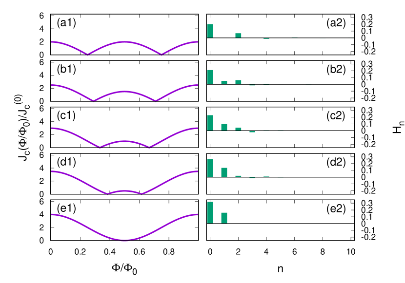
Figure 10: Critical current-flux relations (panel a1-e1) and the corresponding Fourier coefficients (panels a2-e2): The parameters $\alpha_{3TQ_{1}}=\alpha_{3TQ_{2}}=-1$ are used, and $\alpha_{4TSQ}=0,\,-0.5,\,-1,\,\,-1.5,\,-2$ on panels a1-a2, b1-b2, c1-c2, d1-d2 and e1-e2 respectively. The signs of $\alpha_{3TQ_{1}}<0$, $\alpha_{3TQ_{2}}<0$ and $\alpha_{4TSQ}\leq 0$ corresponds to relative $0$-shift between the three-terminal 3TQ₁, 3TQ₂ and the four-terminal 4TSQ.

VIII.3 Conclusion on the Harvard group experimentHarvard-group-experiment

In this subsection, we present the consequences for the Harvard group experiment Harvard-group-experiment .

As it is mentioned above, perturbation theory in the tunnel amplitudes $J_{0}/W$ combined to the adiabatic limit $V=0^{+}$ imply the $\pi$-shifted three-terminal 3TQ₁, 3TQ₂, and $0$-shifted four-terminal 4TSQ, see section V. Given that Eq. (VIII.2) implies Eq. (104), we conclude that perturbation theory and the adiabatic limit imply “Inversion in the critical current $I_{c}(\Phi/\Phi_{0})$ between $\Phi/\Phi_{0}=0$ and $\Phi/\Phi_{0}=1/2$”, i.e. $I_{c}(0)<I_{c}(1/2)$.

Conversely, “Experimental evidence for inversion” implies

“Evidence that the three-terminal 3TQ₁, 3TQ₂ are $\pi$-shifted and the four-terminal 4TSQ are $0$-shifted”,

or, alternatively:

“Evidence for $0$-shifted 3TQ₁, 3TQ₂ and $\pi$-shifted 4TSQ.

No information is gained about which of the three-terminal 3TQ₁, 3TQ₂ or the four-terminal 4TSQ which is $\pi$-shifted, the other being $0$-shifted.

IX Gate voltage dependence of the magnetic field oscillations

IX.1 Notations for the phenomenological model

The previous calculations are summarized in the following phenomenological form of the critical current-flux $\Phi$ relation:

$$J_{c}(\Phi/\Phi_{0}) = J_{c}^{(0)}\mbox{Max}_{\varphi_{q,\,3T}}\left\{\alpha_{3TQ_{1}}\sin\left(\varphi_{q,\,3T}+\Phi\right)\right.$$

$$+ \left.\alpha_{3TQ_{2}}\sin\left(\varphi_{q,\,3T}-\Phi\right)+\alpha_{4TSQ}\sin\varphi_{q,\,3T}\right\},$$

which is deduced from the previous Eq. (VI).

The factorized scaling parameter $J_{c}^{(0)}$ is positive and it has dimension of a critical current. The dimensionless parameters $\alpha_{3TQ_{1}}$, $\alpha_{3TQ_{2}}$ and $\alpha_{4TSQ}$ characterize the relative weights and signs of the three-terminal 3TQ₁, 3TQ₂ and the four-terminal 4TSQ critical currents.

The perturbative calculations presented in the above section V lead to $\alpha_{3TQ_{1}}<0$, $\alpha_{3TQ_{2}}<0$, and to $\alpha_{4TSQ}>0$. Following the previous section VIII, we assume more generally that the three-terminal $\alpha_{3TQ_{1}}$, $\alpha_{3TQ_{2}}$ and the four-terminal $\alpha_{4TSQ}$ can have arbitrary positive or negative relative signs.

General positive or negative signs of $\alpha_{3TQ_{1}}$, $\alpha_{3TQ_{2}}$, and $\alpha_{4TSQ}$ could be relevant to higher transparency of the contacts between the 2D metal and the superconducting leads. However, it has not yet been examined whether increasing the contact transparency via the parameter $J_{0}/W$ can produce change of sign in these coefficients.

IX.2 Analogy with interferometric detection of the $\pi$-shift Guichard

Now, we mention a connection between

(i) The SQUID containing a $0$ and a $\pi$-junction which was realized experimentally in Ref. Guichard, .

(ii) The relative $\pi$-shift between the three-terminal 3TQ₁, 3TQ₂ and the four-terminal 4TSQ.

More specifically:

(i) Half-period shift of the critical current magnetic oscillations is observed in Ref. Guichard, with a SQUID containing a $\pi$-shifted and a $0$-shifted Josephson junction, in comparison with a SQUID containing two $0$-shifted Josephson junctions.

(ii) Half-period shift in the critical current of the four-terminal Josephson junction shown on figures 1 and 3 is produced in our theory when changing “relative shift of $\pi$ between the three-terminal 3TQ₁, 3TQ₂” and the four-terminal 4TSQ into “relative shift of $0$”.

IX.3 Gate voltage dependence of the critical current magnetic oscillations in the perturbative limit

Figures 9 and 10 show on panels a1-e1 the magnetic oscillations of the critical current given by Eq. (IX.1), and their Fourier coefficients $H_{n}$ are shown on panels a2-e2:

$$H_{n}=\int\frac{d\Phi}{2\pi}\cos\left(\frac{2\pi n\Phi}{\Phi_{0}}\right)J_{c}\left(\frac{\Phi}{\Phi_{0}}\right),$$ (108)

where $J_{c}(\Phi/\Phi_{0})$ is given by Eq. (IX.1). The parameters $\alpha_{3TSQ_{1}}=\alpha_{3TSQ_{2}}=-1$ used on figures 9 and 10 have the meaning of the $\pi$-shifted three-terminal 3TQ₁, 3TQ₂ critical currents deduced from perturbation theory in $J_{0}/W$, see section V.

The parameter $\alpha_{4TSQ}>0$ is used on figure 9, thus with $\pi$-shift between the three-terminal 3TQ₁, 3TQ₂ and the four-terminal 4TSQ: $\alpha_{4TSQ}=0$ (panels a1-a2), $\alpha_{4TSQ}=0.5$ (panels b1-b2), $\alpha_{4TSQ}=1$ (panels c1-c2), $\alpha_{4TSQ}=1.5$ (panels d1-d2), and to $\alpha_{4TSQ}=2$ (panels e1-e2).

Figure 10 shows the corresponding data with $\alpha_{4TSQ}<0$ i.e. with and $0$-shift between the three-terminal 3TQ₁, 3TQ₂ and the four-terminal 4TSQ: $\alpha_{4TSQ}=0$ (panels a1-a2), $\alpha_{4TSQ}=-0.5$ (panels b1-b2), $\alpha_{4TSQ}=-1$ (panels c1-c2), $\alpha_{4TSQ}=-1.5$ (panels d1-d2), and to $\alpha_{4TSQ}=-2$ (panels e1-e2).

Figures 9 a1-e1 and figures 10 a1-e1 illustrate the logical chain of Eqs. (104)-(VIII.2): Figures 9 a1-e1 with relative $\pi$-shift between the three-terminal 3TQ₁, 3TQ₂ and the four-terminal 4TSQ reveal the inversion $J_{c}(0)<J_{c}(1/2)$ between $J_{c}(\Phi/\Phi_{0})$ at $\Phi/\Phi_{0}=0$ and $\Phi/\Phi_{0}=1/2$. Conversely, figures 10 a1-e1 with relative $0$-shift feature the noninverted behavior $J_{c}(0)>J_{c}(1/2)$.

In addition, figures 9 and 10 are deduced from each other by half-period shift of $\Phi/2\pi$ on the $x$-axis, which is in agreement with the analogous SQUID containing a $0$- and a $\pi$-shifted Josephson junction, see Ref. Guichard, and the preceding subsection IX.2.

Gating the 2D metal away from the center of the band has the effect of increasing the density of states, which increases $J_{0}/W$ and favors the four-terminal 4TSQ over the three-terminal 3TQ₁, 3TQ₂, because they appear in perturbation at the different orders $(J_{0}/W)^{8}$ and $(J_{0}/W)^{12}$ respectively, see section V.

It is deduced from figures 9 a2-e2 and figures 10 a2-e2 that tuning gate voltage away from the Dirac point increases $|H_{1}|$ and reduces $H_{2}$ [where $H_{1}$ and $H_{2}$ are defined as the $n=1,\,2$ in Eq. (108)], which favors the $\Phi_{0}$ harmonics over the $2\Phi_{0}$ one. Figures 9 and 10 reveal in addition the expected negative $H_{1}<0$ for relative $\pi$-shift between the three-terminal 3TQ₁, 3TQ₂ and the four-terminal 4TSQ, and $H_{1}>0$ for a relative $0$-shift, which is in agreement with the perturbative calculations of section V.

We conclude this section with underlying that our theory is in a qualitative agreement with the Harvard group experimental data Harvard-group-experiment regarding the gate voltage dependence of the critical current magnetic oscillations on the quartet line. Figures 9 and 10 are related to figure 3 in the recent experimental preprint of the Harvard groupHarvard-group-experiment .

X Generalization to arbitrary interface transparencies and finite bias voltage

The three-terminal 3TQ₁, 3TQ₂ transmit even number of Cooper pairs into $S_{{c_{1}}}$ or $S_{{c_{2}}}$ while the four-terminal 4TSQ transmit odd number of Cooper pairs. This characterization based on the parity of the number of Cooper pairs transmitted into $S_{c,1}$ or $S_{c,2}$ is now generalized in the following subsection to arbitrary interface transparencies and finite bias voltage.

Given the arguments of subsection IV.4, we replace the “realistic model I of clean interfaces and superconductors in the dirty limit” by the “physically motivated approximation of the model III”, i.e. clean interfaces and superconductors in the ballistic limit, and averaging over $\{k_{F}R_{k,l}\}$.

We start in subsection X.1 with demonstrating the generalized Ambegaokar-Baratoff formula in the $V=0^{+}$ adiabatic limit at arbitrary interface transparencies. The next subsection X.2 generalizes this argument to finite voltage $V$ on the quartet line, instead of the previous $V=0^{+}$ adiabatic limit. Discussion of the Harvard group experiment Harvard-group-experiment is presented in subsections X.1.2 and X.2.2.

X.1 Generalized Ambegaokar-Baratoff formula in the $V=0^{+}$ adiabatic limit

We start in this subsection with the $V=0^{+}$ adiabatic limit. Subsection X.1.1 demonstrates the generalized Ambegaokar-Baratoff for the quartet current-flux relation, see the forthcoming Eq. (X.1.1). Subsection X.1.2 presents experimental consequences.

X.1.1 Demonstration of the generalized Ambegaokar-Baratoff formula at $V=0^{+}$

Now, we calculate the quartet current in the $V=0^{+}$ adiabatic limit, for arbitrary interface transparencies, and within the model III presented in the above subsection IV.4.

The first term $J_{a,\alpha}\hat{G}_{\alpha,a}^{A}$ appearing in Eq. (42) is written as

$$J_{a,\alpha}\hat{G}_{\alpha,a}^{A} = \sum_{n}\sum_{m_{a},m_{b},m_{c_{1}},m_{c_{2}}}X_{n}^{(m_{a},m_{b},m_{c_{1}},m_{c_{2}}),A}$$

$$\times J_{a}^{2m_{a}}J_{b}^{2m_{b}}J_{{c_{1}}}^{2m_{{c_{1}}}}J_{{c_{2}}}^{2m_{{c_{2}}}}\exp\left(in\varphi_{q,\,3T}\right).$$

Conversely, $J_{a,\alpha}\hat{G}_{\alpha,a}^{R}$ involving the retarded Green’s function takes the form

$$J_{a,\alpha}\hat{G}_{\alpha,a}^{R} = \sum_{n}\sum_{m_{a},m_{b},m_{c_{1}},m_{c_{2}}}X_{n}^{(m_{a},m_{b},m_{c_{1}},m_{c_{2}}),R}$$

$$\times J_{a}^{2m_{a}}J_{b}^{2m_{b}}J_{{c_{1}}}^{2m_{{c_{1}}}}J_{{c_{2}}}^{2m_{{c_{2}}}}\exp\left(in\varphi_{q,\,3T}\right).$$

The bare Green’s functions [i.e. Eqs. (19)-(22) and Eq. (25)] are used to produce a relation between the “advanced” and the “retarded” Green’s functions by taking the complex conjugate and changing the sign of the superconducting phases. This symmetry is then generalized to the fully dressed advanced and retarded Green’s functions by making use of the Dyson Eq. (31). The resulting $\hat{G}^{A}(\omega,R_{0},\psi_{F},\varphi_{N})=\left[\hat{G}^{R}(\omega,R_{0},\psi_{F},-\varphi_{N})\right]^{*}$ leads to

$$X_{n}^{(m_{a},m_{b},m_{c_{1}},m_{c_{2}}),R}=\left[X_{n}^{(m_{a},m_{b},m_{c_{1}},m_{c_{2}}),A}\right]^{*}.$$ (111)

Thus,

$$J_{a,\alpha}\hat{G}_{\alpha,a}^{A}-J_{a,\alpha}\hat{G}_{\alpha,a}^{R}=2i\sum_{n}\sum_{m_{a},m_{b},m_{c_{1}},m_{c_{2}}}$$ (112)

$$\times\mbox{Im}\left[X_{n}^{(m_{a},m_{b},m_{c_{1}},m_{c_{2}}),R}\right]J_{a}^{2m_{a}}J_{b}^{2m_{b}}J_{{c_{1}}}^{2m_{{c_{1}}}}J_{{c_{2}}}^{2m_{{c_{2}}}}\exp\left(in\varphi_{q,\,3T}\right),$$

where the variable $n$ stands for $n\equiv n_{a}=n_{b}$, see the notations in Eq. (56). Eqs. (42)-(45) imply the following decomposition of the critical current in the $V=0^{+}$ adiabatic limit on the quartet line:

$$I^{\prime}_{c}(\Phi/\Phi_{0}) = \mbox{Max}_{\varphi_{c}}\sum_{n,p}X(2n,p)\times$$

$$\sin\left[\left(2n-p\right)\left(\varphi_{c}-\frac{\Phi}{2}\right)+p\left(\varphi_{c}+\frac{\Phi}{2}\right)\right],$$

where the quartet phase is expressed in the gauge given by Eqs. (10) and (11). Eq. (112) shows that the coefficients $X(2n,p)$ appearing in the Ambegaokar-Baratoff formula Eq. (X.1.1) are real-valued. A number $n$ of Cooper pairs is taken from the superconducting lead $S_{a}$ biased at $V_{a}=+V$, and $n$ others pairs are taken from $S_{b}$ biased at $V_{b}=-V$. The integer $p$ in Eq. (X.1.1) denotes partition between the $p$ pairs transmitted into $S_{{c_{2}}}$ contact and the remaining $2n-p$ pairs transmitted into $S_{{c_{1}}}$.

X.1.2 Experimental consequences

In this subsection, we proceed further with the same assumptions as in the preceding subsection X.1.1, and establish a link between:

(i) Emergence of different values for the critical current at fluxes $\Phi/\Phi_{0}=0$ and $\Phi/\Phi_{0}=1/2$ [i.e. $I_{c}(0)\neq I_{c}(1/2)$].

(ii) Evidence for interference between quantum processes transmitting even or odd numbers of Cooper pairs into $S_{{c_{1}}}$ or $S_{{c_{2}}}$.

Specifically, we make the change of variables $\varphi_{c}\rightarrow\varphi_{c}+\Phi/2$ in Eq. (X.1.1), which is equivalent to changing the gauge from Eqs. (10)-(11) to $\varphi_{{c_{1}}}=\varphi_{c}$ and $\varphi_{{c_{2}}}=\varphi_{c}+\Phi$:

$$I^{\prime}_{c}(\Phi/\Phi_{0})=\mbox{Max}_{\varphi_{c}}\sum_{n,p}X(2n,p)\sin\left[\left(2n-p\right)\varphi_{c}+p\left(\varphi_{c}+\Phi\right)\right].$$ (114)

This Eq. (114) simplifies as

$$I^{\prime}_{c}(\Phi/\Phi_{0})=\mbox{Max}_{\varphi_{c}}\sum_{n,p}X(2n,p)\sin\left[2n\varphi_{c}+p\Phi\right].$$ (115)

It deduced that

$$I^{\prime}_{c}(0) = \mbox{Max}_{\varphi_{c}}\sum_{n,p}X(2n,p)\sin\left[2n\varphi_{c}\right]$$ (116)

$$I^{\prime}_{c}(1/2) = \mbox{Max}_{\varphi_{c}}\sum_{n,p}X(2n,p)(-)^{p}\sin\left[2n\varphi_{c}\right].$$ (117)

Separating the terms with $p$ even or odd according to

$$Y_{even}(\varphi_{c})=\sum_{p\,even}\sum_{n}X(2n,p)\sin\left[2n\varphi_{c}\right]$$ (118)

$$Y_{odd}(\varphi_{c})=\sum_{p\,odd}\sum_{n}X(2n,p)\sin\left[2n\varphi_{c}\right]$$ (119)

leads to

$$I^{\prime}_{c}(0) = \mbox{Max}_{\varphi_{c}}\left[Y_{even}(\varphi_{c})+Y_{odd}(\varphi_{c})\right]$$ (120)

$$I^{\prime}_{c}(1/2) = \mbox{Max}_{\varphi_{c}}\left[Y_{even}(\varphi_{c})-Y_{odd}(\varphi_{c})\right].$$ (121)

The following logical link is deduced within the assumptions mentioned above:

“Experimental observation for different values of the critical current between reduced fluxes $\Phi/\Phi_{0}=0$ and $\Phi/\Phi_{0}=1/2$ at arbitrary transparency” [i.e. $I^{\prime}_{c}(0)\neq I^{\prime}_{c}(1/2)$ in Eqs. (120) and (121)]

is equivalent to

“Evidence for interference between processes transmitting even or odd number of Cooper pairs into $S_{{c_{1}}}$ and $S_{{c_{2}}}$”.

X.2 Generalization to finite bias voltage on the quartet line

Now, we generalize to finite bias voltage $V$ and arbitrary interface transparencies. Disorder is treated within the model III introduced in subsection IV.4.

Specifically, we show in subsection X.2.1 that the Ambegaokar-Baratoff formula Eq. (X.1.1) holds at finite $V$ within our treatment. Consequences for the proposed interpretation of the Harvard group experiment are discussed in subsection X.2.2.

X.2.1 Demonstration of the Ambegaokar-Baratoff formula at finite bias voltage

Now, at finite bias voltage $V$ on the quartet line, we show that the currents transmitted at the $S_{c,1}$ or $S_{c,2}$ contacts take the form of the generalized Ambegaokar-Baratoff formula Eq. (X.1.1), where the coefficients $X(2n,p)$ appearing in the $V=0^{+}$ Eq. (X.1.1) are replaced by their values $X(2n,p,eV/\Delta)$ at finite bias voltage $V$.

The Keldysh Green’s function given by Eq. (35) is written as $\hat{G}^{+,-}=\hat{G}^{+,-}_{A}+\hat{G}^{+,-}_{B}$, where the “quasiequilibrium” and the “nonequilibrium” $\hat{G}^{+,-}_{A}$ and $\hat{G}^{+,-}_{B}$ are given by

$$\hat{G}^{+,-}_{A} = \hat{n}_{F}\hat{G}^{A}-\hat{G}^{R}\hat{n}_{F}$$ (122)

$$\hat{G}^{+,-}_{B} = \hat{G}^{R}\left[\hat{J}\hat{n}_{F}-\hat{n}_{F}\hat{J}\right]\hat{G}^{A}$$ (123)

respectively. The matrices appearing in Eqs. (122)-(123) are now defined both in Nambu and in the infinite set of harmonics of the Josephson frequencies. In the following, we use the notations $\check{\varphi}=(\varphi_{a},\varphi_{b},\varphi_{c,1},\varphi_{c,2})$ for the superconducting phases and ${\check{n}}=(n_{a},n_{b},n_{c,1},n_{c,2})$ for labeling the multiples of the voltage frequency $eV/\hbar$. The $\check{n}$ vector belongs to the set $S_{\check{n}}$ of quadruplets which fulfill the constraints

$$n_{a}+n_{b}+n_{c,1}+n_{c,2}=0$$ (124)

$$n_{a}=n_{b},$$ (125)

see the discussion following Eq. (56).

We start with the quasiequilibrium contribution $I_{A}$ deduced from Eqs. (40)-(40):

$$-I_{A}\equiv-I_{A,\gamma_{c_{1}}\rightarrow c_{1}}=\frac{e}{\hbar}\sum_{p}\int d\omega$$

$$\left\{\left[\hat{J}_{c_{1,p},\gamma_{c_{1,p}}}\hat{G}^{+,-}_{A,\gamma_{c_{1,p}},c_{1,p}}\right]_{(1,1)/(0,0)}(\omega,\check{\varphi},\{\psi_{F,k,l}\},V)\right.$$ (126)

$$-\left[\hat{J}_{c_{1,p},\gamma_{c_{1,p}}}\hat{G}^{+,-}_{A,\gamma_{c_{1,p}},c_{1,p}}\right]_{(2,2)/(0,0)}(\omega,\check{\varphi},\{\psi_{F,k,l}\},V)$$ (127)

$$-\left[\hat{J}_{\gamma_{c_{1,p}},c_{1,p}}\hat{G}^{+,-}_{A,c_{1,p},\gamma_{c_{1,p}}}\right]_{(1,1)/(0,0)}(\omega,\check{\varphi},\{\psi_{F,k,l}\},V)$$ (128)

$$+\left.\left[\hat{J}_{\gamma_{c_{1,p}},c_{1,p}}\hat{G}^{+,-}_{A,c_{1,p},\gamma_{c_{1,p}}}\right]_{(2,2)/(0,0)}(\omega,\check{\varphi},\{\psi_{F,k,l}\},V)\right\},$$ (129)

where $\hat{G}^{+,-}_{A}$ is given by Eq. (122). The notation $\{\psi_{F,k,l}\}$ stands for the phases oscillating at the scale of the Fermi wave-length in a multichannel configuration, as they appear in the 2D metal and superconductor Green’s functions, see Eqs. (19)-(22) and Eq. (25) respectively. Namely, $\psi_{F,k,l}=k_{F}R_{k,l}-\pi/4$ for the 2D metal, see Eqs. (19)-(22), and $\psi_{F,k,l}=k_{F}R_{k,l}$ for the ballistic 3D superconductors, see Eq. (25).

The Dyson Eq. (31) implies that the fully dressed advanced and retarded Green’s functions take the following form:

$$\hat{G}^{A}\left(\omega,\check{\varphi},\{\psi_{F,k,l}\},V\right) = \sum_{\check{n}\in S_{\check{n}}}\hat{G}^{A}_{\check{n}}\left(\omega,\{\psi_{F,k,l}\},V\right)e^{i{\check{n}}.\check{\varphi}}$$ (130)

$$\hat{G}^{R}\left(\omega,\check{\varphi},\{k_{F}R_{k,l}\}\right) = \sum_{\check{n}\in S_{\check{n}}}\hat{G}^{R}_{\check{n}}\left(\omega,\{\psi_{F,k,l}\}\right)e^{i{\check{n}}.\check{\varphi}}.$$ (131)

In order to relate $\hat{G}^{A}_{\check{n}}$ to $\hat{G}^{R}_{\check{n}}$ in Eqs. (130) and (131), we note that the bare Green’s functions given by Eqs. (19)-(22) and Eq. (25) are such that

$$\hat{\cal T}_{Nambu}\hat{g}^{A,R}\left(\omega,\check{\varphi},\{\psi_{F,k,l}\},V\right)=\hat{g}^{A,R}\left(\omega,-\check{\varphi},\{-\psi_{F,k,l}\},-V\right),$$ (132)

where the transformation $\hat{\cal T}_{Nambu}$ exchanges the “1” and “2” Nambu components for “spin-up electron” and “spin-down hole” respectively. The Dyson equation given by Eq. (31) yields

$$\hat{\cal T}_{Nambu}\hat{J}_{a,\gamma_{c_{1}}}\hat{G}^{A,R}_{\gamma_{c_{1}},c_{1}}\left(\omega,\check{\varphi},\{\psi_{F,k,l}\},V\right)$$

$$= \hat{J}_{a,\gamma_{c_{1}}}\hat{G}^{A,R}_{\gamma_{c_{1}},c_{1}}\left(\omega,-\check{\varphi},\{-\psi_{F,k,l}\},-V\right).$$

Combining Eq. (122) to Eq. (X.2.1) leads to

$$\sum_{p}\int d\omega n_{F}(\omega)\left\{\langle\langle\hat{J}_{c_{1,p},\gamma_{c_{1,p}}}\hat{G}^{A}_{\gamma_{c_{1,p}},c_{1,p}}\left(\omega,\{\psi_{F,k,l}\},V,\check{\varphi}\right)\rangle\rangle_{(1,1)}\right.$$

$$-\left.\langle\langle\hat{J}_{c_{1,p},\gamma_{c_{1,p}}}\hat{G}^{A}_{\gamma_{c_{1,p}},c_{1,p}}\left(\omega,\{\psi_{F,k,l}\},-V,\check{\varphi}\}\right)\rangle\rangle_{(2,2)}\right\}$$

$$=2i\sum_{p}\int d\omega n_{F}(\omega)\sum_{\check{n}\in S_{\check{n}}}$$ (134)

$$\langle\langle\hat{J}_{c_{1,p},\gamma_{c_{1,p}}}\mbox{Im}\left[G^{A}_{\gamma_{c_{1,p}},c_{1,p},{\check{n}}}\left(\omega,\{\psi_{F,k,l}\},V\right)\right]\rangle\rangle_{(1,1)}\sin\left({\check{n}}.\check{\varphi}\right).$$

Within the considered model III, averaging over disorder is mimicked by integrating over the phases $\{\psi_{F,k,l}\}$ in the $\left[0,2\pi\right]$ interval. The terms which are odd in $k_{F}R_{k,l}$ do not contribute to this integral, and thus

$$\langle\langle\hat{J}_{c_{1,p},\gamma_{c_{1,p}}}\hat{G}^{A}_{\gamma_{c_{1,p}},c_{1,p}}(\omega,\check{\varphi},\{\psi_{F,k,l}\},V)\rangle\rangle_{(1,1)}$$

$$= \langle\langle\hat{J}_{c_{1,p},\gamma_{c_{1,p}}}\hat{G}^{A}_{\gamma_{c_{1,p}},c_{1,p}}(\omega,-\check{\varphi},\{\psi_{F,k,l}\},-V)\rangle\rangle_{(2,2)}$$

is independent on whether $\hat{G}^{A}_{\gamma_{c_{1,p}},c_{1,p}}(\omega,-\check{\varphi},\{\psi_{F,k,l}\},V)$ or $\hat{G}^{A}_{\gamma_{c_{1,p}},c_{1,p}}(\omega,-\check{\varphi},\{-\psi_{F,k,l}\},V)$ is averaged over $\{\psi_{F,k,l}\}$. In addition, the calculation is specific to the “quartet current” $I_{q}$ which is even if the voltage $V$ changes sign.

The subtracted “retarded” terms are deduced from the “advanced” ones by taking the complex conjugate and changing $\check{\varphi}$ into $-\check{\varphi}$, see subsection X.1.1. We deduce the following expression of $\langle\langle I_{A}\rangle\rangle$:

$$\langle\langle I_{q,A}\rangle\rangle = \frac{2e}{\hbar}\sum_{p}\int d\omega n_{F}(\omega)\sum_{\check{n}\in S_{\check{n}}}$$

$$\mbox{Im}\langle\langle J_{c_{1,p},\gamma_{c_{1,p}}}G^{A}_{{\check{n}},\gamma_{c_{1,p}},c_{1,p}}\left(\omega,\{\psi_{F,k,l}\},V\right)\rangle\rangle\sin\left({\check{n}}.\check{\varphi}\right)$$

$$+ \left(V\rightarrow-V\right),$$

which takes the form of the Ambegaokar-Baratoff formula Eq. (X.1.1) for $I_{q,A}(V)=[I_{A}(V)+I_{A}(-V)]/2$.

Now, Eqs. (40)-(40) and Eq. (123) yield the following “nonequilibrium” contribution $I_{B}$ to the current:

$$-I_{B}\equiv-I_{B,\gamma_{c_{1}}\rightarrow c_{1}}=\frac{e}{\hbar}\sum_{p}\int d\omega$$

$$\left\{\left[\hat{J}_{c_{1,p},\gamma_{c_{1,p}}}\hat{G}^{+,-}_{B,\gamma_{c_{1,p}},c_{1,p}}\right]_{(1,1)/(0,0)}(\omega,\check{\varphi},\{\psi_{F,k,l}\},V)\right.$$ (137)

$$-\left[\hat{J}_{c_{1,p},\gamma_{c_{1,p}}}\hat{G}^{+,-}_{B,\gamma_{c_{1,p}},c_{1,p}}\right]_{(2,2)/(0,0)}(\omega,\check{\varphi},\{\psi_{F,k,l}\},V)$$ (138)

$$-\left[\hat{J}_{\gamma_{c_{1,p}},c_{1,p}}\hat{G}^{+,-}_{B,c_{1,p},\gamma_{c_{1,p}}}\right]_{(1,1)/(0,0)}(\omega,\check{\varphi},\{\psi_{F,k,l}\},V)$$ (139)

$$+\left.\left[\hat{J}_{\gamma_{c_{1,p}},c_{1,p}}\hat{G}^{+,-}_{B,c_{1,p},\gamma_{c_{1,p}}}\right]_{(2,2)/(0,0)}(\omega,\check{\varphi},\{\psi_{F,k,l}\},V)\right\},$$ (140)

where $\hat{G}^{+,-}_{B}$ is given by Eq. (123).

We make use of the transformation ${\cal T}_{Nambu}$ given by Eq. (132) to obtain

$$\left[\hat{J}_{c_{1,p},\gamma_{c_{1,p}}}\hat{G}^{+,-}_{B,\gamma_{c_{1,p}},c_{1,p}}\right]_{(1,1)/(0,0)}(\omega,\check{\varphi},\{\psi_{F,k,l}\},V)$$ (141)

$$- \left[\hat{J}_{c_{1,p},\gamma_{c_{1,p}}}\hat{G}^{+,-}_{B,\gamma_{c_{1,p}},c_{1,p}}\right]_{(2,2)/(0,0)}(\omega,\check{\varphi},\{\psi_{F,k,l}\},-V)$$

$$= 2i\sum_{\check{n}\in S_{\check{n}}}\left[\hat{J}_{c_{1,p},\gamma_{c_{1,p}}}\hat{G}^{+,-}_{B,\gamma_{c_{1,p}},c_{1,p},\check{n}}\right]_{(1,1)/(0,0)}(\omega,\check{\varphi},\{\psi_{F,k,l}\},V)$$

$$\times\sin\left(\check{n}.\check{\varphi}\right).$$

Now, we note that $\hat{J}^{\dagger}=\hat{J}$ combined to

$$\left[\hat{g}^{A,R}\left(\omega,\check{\varphi},\{\psi_{F,k,l}\},V\right)\right]^{\dagger}=\hat{g}^{R,A}\left(\omega,\check{\varphi},\{\psi_{F,k,l}\},V\right)$$ (142)

and to the Dyson Eq. (31) leads to $\left(\hat{G}^{A,R}\right)^{\dagger}=\hat{G}^{R,A}$. Conversely, combining to Eq. (123) yields $\left(\hat{G}^{+,-}_{B}\right)^{\dagger}=\hat{G}^{+,-}_{B}$. We deduce that $\langle\langle I_{q,B}\rangle\rangle$ takes the following form of the Ambegaokar-Baratoff formula

$$\langle\langle I_{q,B}\rangle\rangle = \frac{2e}{\hbar}\sum_{p}\int d\omega n_{F}(\omega)\sum_{\check{n}\in S_{\check{n}}}$$

$$\mbox{Im}\langle\langle J_{c_{1,p},\gamma_{c_{1,p}}}G^{+,-}_{B,{\check{n}},\gamma_{c_{1,p}},c_{1,p}}\left(\omega,\{\psi_{F,k,l}\},V\right)\rangle\rangle\sin\left({\check{n}}.\check{\varphi}\right)$$

$$+ \left(V\rightarrow-V\right),$$

where $I_{q,B}(V)=[I_{B}(V)+I_{B}(-V)]/2$.

It is concluded that both Eq. (X.2.1) for the “quasi-equilibrium quartet current” $\langle\langle I_{q,A}\rangle\rangle$ entering or exiting $S_{c,1}$ and Eq. (X.2.1) for the “nonequilibrium quartet current” $\langle\langle I_{q,B}\rangle\rangle$ take the form of the “generalized Ambegaokar-Baratoff formula” Eq. (X.1.1) where the coefficients $X(2n,p)$ acquire a dependence on the voltage $V$.

X.2.2 Conclusion on the Harvard group experiment Harvard-group-experiment

It deduced that the assumption of arbitrary interface transparencies and finite bias voltage $V$, combined to mimicking disorder in the superconducting leads by averaging over $\{k_{F}R_{k,l}\}$, leads to the following statement:

“Experimental evidence for $I^{\prime}_{c}(0)\neq I^{\prime}_{c}(1/2)$” implies “Evidence for transmission of odd number of Cooper pairs into $S_{{c_{1}}}$ or $S_{{c_{2}}}$”.

This statement implies “Evidence for microscopic processes containing odd number of electron-hole or hole-electron conversions in lead $S_{c,1}$.”

Going one step further, we note that multiple quartet superconducting diffusion modes of the $\langle\langle g_{(1,2)}g_{(1,2)}\rangle\rangle$-type in Eqs. (IV.3) and (58) necessarily imply even numbers of electron-hole or hole-electron conversions. Thus, the requirement of odd number of electron-hole or hole-electron conversions in lead $S_{c,1}$ implies that at least one $\langle\langle g_{(1,1)}g_{(1,2)}\rangle\rangle$ mode of the 4TSQ-type is involved in the corresponding diagram, see Eqs. (IV.3) and (59).

This argument relies on gathering the nonlocal Green’s functions in a pair-wise manner. It would break down for localized contacts such that $r_{0}\lesssim l_{e}$, because the unpaired “local” electron-hole conversions would have to be taken into account on the same footing as the pairs of nonlocal Green’s functions.

The paper is concluded with the following remark regarding the Harvard group experiment Harvard-group-experiment :

“Experimental evidence for different values of the critical currents between $\Phi/\Phi_{0}=0$ and $\Phi/\Phi_{0}=1/2$ ”, i.e. $I^{\prime}_{c}(0)\neq I^{\prime}_{c}(1/2)$

implies

“Evidence for the four-terminal 4TSQ”.

This statement holds for arbitrary device parameters and it was demonstrated within the physically motivated approximation of the model III discussed in the above subsection IV.4.

XI Conclusions

Now, we provide a summary of the paper in subsection XI.1, specific conclusions on the Harvard group experiment in subsection XI.2 and final remarks and outlook in subsection XI.3.

XI.1 Summary of the paper

In this paper, we provided a possible mechanism for the inversion in the critical current $I_{c}(\Phi/\Phi_{0})$ on the quartet line in a four-terminal Josephson junction (see figures 1 and 3), in connection with the recent Harvard group experiment Harvard-group-experiment .

The Harvard group experiment Harvard-group-experiment uses graphene gated away from the Dirac point, which was modeled as a simple 2D metal with circular Fermi surface. We took the two dimensions of the graphene sheet into account while ignoring the effects related to the Dirac cones.

Specifically, we calculated microscopically the Josephson relations from lowest-order perturbation theory in the tunnel amplitudes, assuming in addition the adiabatic limit. We found that the three- and four-terminal quartet channels interfere with each other in the critical current on the quartet line. The “standard” three-terminal 3TQ₁ transmit two pairs into $S_{c,1}$ and the three-terminal 3TQ₂ transmit two pairs into $S_{c,2}$. The nonstandard four-terminal 4TSQ transmit two Coopers in the same quantum process but in a split manner, i.e. one pair into $S_{c,1}$ and the other one into $S_{c,2}$.

We found that the four-terminal 4TSQ do not contribute to the dc-current if a 1D or a 3D metal and multichannel contacts are used instead of the considered 2D metal. The importance of 2D is related to the general properties of the solutions of the wave equation, which imply a wake in even dimension (such as 2D), but not in odd dimension (such as 1D or 3D). We demonstrated that the “2D quantum wake” can synchronize two Josephson junctions by the exchange of a quasiparticle at the $S_{{c_{1}}}$ and $S_{{c_{2}}}$ contacts, yielding a nonvanishingly small four-terminal 4TSQ critical current.

We demonstrated that, with a 2D metal, lowest-order perturbation theory and the adiabatic limit produce $\pi$- and $0$-shifted current-phase relations for the three-terminal 3TQ₁, 3TQ₂ and for the four-terminal 4TSQ respectively. This implies inversion $I_{c}(0)<I_{c}(1/2)$ between the critical currents $I_{c}(0)$ and $I_{c}(1/2)$ at fluxes $\Phi/\Phi_{0}=0$ and $\Phi/\Phi_{0}=1/2$ respectively. In turn, experimental evidence for inversion implies $(\pi,0)$ or $(0,\pi)$ shifts for the three-terminal 3TQ₁, 3TQ₂ and the four-terminal 4TSQ respectively. This type of experiment cannot determine which of the three-terminal 3TQ₁, 3TQ₂ or the four-terminal 4TSQ is $\pi$-shifted, the other being $0$-shifted.

We proposed an analogy with experiments on a SQUID containing $\pi$- and $0$-shifted Josephson junctions Guichard . In this analogy with Ref. Guichard, , the $\pi$- and $0$-shifted three-terminal 3TQ₁, 3TQ₂ and the four-terminal 4TSQ play the role of the $\pi$- or $0$-shifted two-terminal Josephson junctions inserted in the SQUID loop respectively.

In addition, the perturbative calculation predicts that the relative weight of the three-terminal 3TQ₁, 3TQ₂ and the four-terminal 4TSQ changes with gate voltage on the 2D metal, in a way which is compatible with the experimental data of the Harvard group Harvard-group-experiment .

We also generalized our theory to arbitrary interface transparencies and finite bias voltage $V$ on the quartet line. This generalization was based on the even or odd parity of the number of Cooper pairs transmitted into $S_{c,1}$ or $S_{c,2}$ by the three-terminal 3TQ₁, 3TQ₂ and the four-terminal 4TSQ.

We treated the ingredients of “arbitrary interface transparencies” and “finite bias voltage” within a physically-motivated approximation for disorder. The current entering or exiting $S_{c,1}$ takes the form of the generalized Ambegaokar-Baratoff relation from which we could infer that the 4TSQ imply different values for critical current $I_{c}(\Phi/\Phi_{0})$ at $\Phi/\Phi_{0}=0$ and $\Phi/\Phi_{0}=1/2$. We argued within this framework of physically-motivated approximation that “$I_{c}(0)\neq I_{c}(1/2)$” implies “Evidence for the nonstandard four-terminal 4TSQ”.

XI.2 Specific conclusion on the Harvard group experiment Harvard-group-experiment

To summarize, our theory teaches the following on the Harvard group experimental data Harvard-group-experiment :

(i) Perturbation theory in the tunnel amplitudes combined to the $V=0^{+}$ adiabatic limit produces the “Inversion in $I_{c}(\Phi/\Phi_{0})$ between $\Phi/\Phi_{0}=0$ and $\Phi/\Phi_{0}=1/2$” which is observed in the Harvard group experiment Harvard-group-experiment .

(ii) The calculated gate voltage dependence of the critical current oscillations as a function of magnetic field is compatible with the Harvard group experimental results Harvard-group-experiment .

(iii) We argued that “Experimental evidence for $I_{c}(0)\neq I_{c}(1/2)$” implies “Evidence for the four-terminal 4TSQ”. Thus, our model implies that the Harvard group experiment Harvard-group-experiment is evidence for the four-terminal 4TSQ.

XI.3 Final remarks and outlook

The four-terminal 4TSQ shown on figures 6c, d and on figure 8 are robust against taking the long junction limit $R_{0}/x_{0}\lesssim l_{\varphi}$ along the $x$-axis direction, where $l_{\varphi}$ is the mesoscopic phase coherence length of the 2D metal. It is assumed in addition that the device remains short along the $y$-direction, i.e. $R_{0}/y_{0}\lesssim\xi_{dirty}(0)$. The device geometry is shown on figure 3.

More precisely, the nonlocal $\langle\langle{g_{(1,1)}g_{(1,1)}}\rangle\rangle$ mode connects $S_{c,1}$ and $S_{c,2}$ through the 2D metal by the quantum wake, see the highlighted section of the four-terminal 4TSQ diagram on figure 6d. Eq. (19) provides the expression of each single-particle Green’s function $g_{(1,1)}$ entering the $\langle\langle{g_{(1,1)}g_{(1,1)}}\rangle\rangle$ mode through the 2D metal. Both nonlocal $g_{(1,1)}$ are in the “electron-electron” channel and they are both evaluated at the same wave-vector $k_{e}=k_{F}+\omega/v_{F}$. Thus, $\langle\langle{g_{(1,1)}g_{(1,1)}}\rangle\rangle$ is not washed out by multichannel averaging if the energy $\omega$ is larger than the Thouless energy $\hbar v_{F}/R$ associated to the separation $R$ between the contacts. This is why the four-terminal 4TSQ critical current given by the diagram on figure 8d remains large as long as the device dimension $R_{0}/x_{0}$ along the $x$-axis is in the mesoscopic domain, i.e. $R_{0}/x_{0}\lesssim l_{\varphi}$.

In addition, the $V=0$ limit of phase-biased superconductors (instead of the $V=0^{+}$ adiabatic limit of a voltage-biased device) also involves long-distance coupling between the Andreev bound states associated to each pair of Josephson junctions sharing a 2D metal as a common weak link, according to to $R_{0}/x_{0}\lesssim l_{\varphi}$ mentioned above in the geometry on figure 3.

These arguments show that the four-terminal 4TSQ constitute a nonstandard “mesoscopic” channel of quantum coherent synchronization, which operates in between the quartets at the smallest scale and the early 1980s synchronization of macroscopic Josephson circuits NJ1 ; NJ2 . An interesting complementary point of view is to approach this mesoscopic regime from the classical limit, i.e. to incorporate quantum fluctuation in the classical circuit models.

We also note that comparing Eq. (73) for the three-terminal 3TQ₁ critical current $I_{c,\,3TQ_{1}}$ to Eq. (92) for the four-terminal 4TSQ critical current $I_{c,\,4TSQ}^{(2)}$ leads to the following order of magnitude for their ratio:

$$K=\left|\frac{I_{c,\,4TSQ}^{(2)}}{I_{c,\,3TQ_{1}}}\right|\approx\left(\frac{J_{0}}{W}\right)^{4}\frac{\sqrt{{\cal S}_{contact}}}{l_{e}}.$$ (144)

It was assumed implicitly in this paper I that perturbation theory is converging, which implies $K<1$. Paper III of the series will address resummations of the perturbative expansions if the diffusion modes proliferate for $K>1$.

Finally, we point out that, in the presence of Coulomb interactions, the charging energy is larger for the three-terminal 3TQ₁ and 3TQ₂ (involving four fermions in $S_{c,1}$ or four fermions in $S_{c,2}$) than for the four-terminal 4TSQ (involving one pair in $S_{c,1}$ and another one in $S_{c,2}$). Thus, static Coulomb interactions favor the nonstandard four-terminal 4TSQ over the three-terminal 3TQ₁, 3TQ₂. It would be interesting to address dynamical Coulomb blockade Levy-Yeyati for the device in figures 1 and 3.

Appendix A Green’s function of a 2D metal

We start this Appendix with the Fourier transform of the Green’s function between two tight-binding sites separated by distance $R$:

$$g^{A,(1,1)/(2,2)}(R,\omega)=$$ (145)

$$\int_{-\pi}^{\pi}d\theta\int_{0}^{+\infty}\frac{kdk}{(2\pi)^{2}}\exp\left(ikR\cos\theta\right)g^{A,(1,1)/(2,2)}({\bf k},\omega),$$

where

$$g^{A,(1,1)}({\bf k},\omega) = \frac{1}{\omega-\xi_{\bf k}-i\eta}$$ (146)

$$g^{A,(2,2)}({\bf k},\omega) = \frac{1}{\omega+\xi_{\bf k}-i\eta},$$ (147)

with $\xi_{\bf k}$ the kinetic energy of the 2D plane-wave state ${\bf k}$ with respect to the chemical potential $\mu=\hbar^{2}k_{F}^{2}/2m$, and where $k_{F}$ and $m$ are the Fermi wave-vector and the band-mass respectively. The superscripts “$(1,1)$” or “$(2,2)$” in Eqs. (145)-(147) refer to propagation in the electron-electron or hole-hole channels respectively.

Eq. (145) is written as

$$g^{A}(R,\omega)=\int_{0}^{+\infty}\frac{kdk}{(2\pi)}\frac{J_{0}(kR)}{\omega-\epsilon\xi_{\bf k}-i\eta},$$ (148)

where the Bessel function

$$J_{0}(x)=\frac{1}{2\pi}\int_{-\pi}^{\pi}\exp\left(ix\cos\theta\right)d\theta$$ (149)

was introduced in Eq. (148). The parameter $\epsilon$ takes the values $\epsilon=\pm 1$ for the $(1,1)$ and $(2,2)$ components respectively. We consider a pole at

$$k\equiv k_{0}\simeq k_{F}+\frac{\epsilon(\omega-i\eta)}{v_{F}}$$ (150)

and the residue is evaluated according to

$$\omega-\epsilon\xi_{k_{0}+\delta k}-i\eta\simeq-\frac{\hbar^{2}}{2m}\epsilon k_{0}\delta k\simeq-\epsilon v_{F}k_{0}\delta k.$$ (151)

Considering in addition that $\mbox{sign}\left(\mbox{Im}k_{0}\right)=-\epsilon$ and using contour integration in the complex $k$ plane leads to

$$g^{A,(1,1)}(R) = g^{A,(2,2)}(R)=\frac{i}{W}J_{0}(k_{F}R)$$ (152)

$$g^{R,(1,1)}(R) = g^{R,(2,2)}(R)=-\frac{i}{W}J_{0}(k_{F}R),$$ (153)

where the limit $\omega R/v_{F}\lesssim 1$ is considered. Noting that $\omega$ has typical order of magnitude set by the superconducting gap, the condition $\omega R/v_{F}\lesssim 1$ yields the short junction limit $R\lesssim\xi_{ball}(0)$ for each pair of superconductor-2D metal-superconductor Josephson junction, where the ballistic superconducting coherence length is given by Eq. ( 5) and Eq. (29).

Eqs. (152)-(153) lead to Eqs. (19)-(22) if the realistic condition $2\pi/k_{F}\ll R\lesssim\xi_{ball}(0)$ is fulfilled on the separation $R$.

Appendix B Superconducting diffusion modes in the dirty limit

The goal of this Appendix is to treat disorder in the superconducting leads of the considered four-terminal device. The calculations are based on Ref. Smith-Ambegaokar, .

Averaging the one-particle Green’s functions over disorder in the Born approximation is summarized in subsection B.1. Subsection B.2 presents the calculation of the disorder-averaged superconducting modes in the dirty limit.

The superconducting modes are formed with products of Nambu Green’s functions scattering together on the same configuration of disorder, see subsection IV.3.

Now, the superconducting diffusion modes are calculated in the ladder approximation.

B.1 One-particle Green’s function averaged over disorder

We start with the expression of the average over disorder of the one-particle Green’s functions Abrikosov .

Using the notations of Ref. Smith-Ambegaokar, , the average superconducting Green’s function takes the following form in the Born approximation:

$$\hat{g}^{A,R}(\xi_{\bf k},\omega)=\frac{\hat{\cal N}_{\bf k}(\omega)}{{\cal D}_{\bf k}(\omega)},$$ (154)

with

$$\hat{\cal N}_{\bf k}(\omega) = \overline{\omega}\mp i\eta+\xi_{\bf k}\hat{\tau}_{3}+\overline{\Delta}\hat{\tau}_{1}$$ (155)

$${\cal D}_{\bf k}(\omega) = \left(\overline{\omega}\mp i\eta\right)^{2}-\overline{\Delta}^{2}-\xi_{\bf k}^{2},$$ (156)

where $\omega$ and ${\bf k}$ refer to the energy and wave-vector respectively. The notations $\overline{\omega}$, $\overline{\Delta}$ and $s(\omega)$ stand for

$$\overline{\omega} = \omega\left(1+\frac{1}{s(\omega)\tau}\right)$$ (157)

$$\overline{\Delta} = \Delta\left(1+\frac{1}{s(\omega)\tau}\right)$$ (158)

$$s^{2}(\omega) = \Delta^{2}-\omega^{2}.$$ (159)

B.2 Product of two Green’s function averaged over disorder

Now, we evaluate the average over disorder of the product of two Nambu Green’s functions. An intermediate result on two integrals is presented in subsection B.2.1. The resummations of the ladders is presented in subsection B.2.2.

B.2.1 Intermediate result on evaluation of useful integrals

Following Ref. Smith-Ambegaokar, , we evaluate the following integrals at energy $|\omega|<\Delta$ within the gap:

$${\cal I}_{\alpha}^{A,A}({\bf q},\omega)$$

$$= v^{2}\int\frac{d{\bf k}}{(2\pi)^{3}}\hat{\tau}_{3}\hat{g}^{A}({\xi}_{\bf k},\omega)\hat{\tau}_{\alpha}\hat{g}^{A}(\xi_{{\bf k}+{\bf q}},\omega)\hat{\tau}_{3}$$

$${\cal I}_{\alpha}^{A,R}({\bf q},\omega)$$

$$= v^{2}\int\frac{d{\bf k}}{(2\pi)^{3}}\hat{\tau}_{3}\hat{g}^{A}({\xi}_{\bf k},\omega)\hat{\tau}_{\alpha}\hat{g}^{R}(\xi_{{\bf k}+{\bf q}},\omega)\hat{\tau}_{3},$$

where $\hat{\tau}_{\alpha}$ are the $2\times 2$ Pauli matrices.

The first step of the calculation is to combine the relation

$$\int\frac{d{\bf k}}{(2\pi)^{3}}=\frac{1}{8\pi^{2}}\int_{-1}^{1}du\int_{-\infty}^{+\infty}k^{2}dk\exp(ikRu)$$ (162)

to contour integration for the integral over $k$.

The poles of $\hat{g}^{A}({\xi}_{\bf k},\omega)$ are given by the solutions of ${\cal D}_{\bf k}^{A}(\omega)=0$ at $k=k_{0}$, namely

$$\xi_{{\bf k}_{0}}^{2}=\overline{\omega}^{2}-\overline{\Delta}^{2}-2i\eta\overline{\omega}=0.$$ (163)

A branch-cut along the $\omega<0$ axis leads to

$$\xi_{{\bf k}_{0}}^{(\epsilon)}(\omega)=i\epsilon\sqrt{\overline{\Delta}^{2}-\overline{\omega}^{2}},$$ (164)

with

$$\epsilon=\mbox{sgn}\left(-\eta\overline{\omega}\right).$$ (165)

The solutions of Eq. (164) for $k_{0}>0$ or $k_{0}<0$ are given by

$$k_{0}^{(\epsilon,\epsilon^{\prime})}(\omega)=\epsilon^{\prime}\left(k_{F}+\frac{i\epsilon\overline{s}(\omega)}{\hbar v_{F}}\right),$$ (166)

with $\epsilon^{\prime}=\pm$.

No reason is advocated for why a constraint holds between $\mbox{Re}\left[k_{0}(\omega)\right]$ and $\mbox{Im}\left[k_{0}(\omega)\right]$. Instead, the four solutions are relevant to a double interface, i.e. those with exponential growth or decay along the positive or negative directions of propagation. For instance, the four waves are involved in the solution of the Bogoliubov-de Gennes equations within the Blonder-Tinkham-Klapwijk approach BTK for a normal metal-superconductor-normal metal double junction Floser , with separation between the contacts comparable to the superconducting coherence length. Thus, the four wave-vectors $k_{0}^{(\epsilon,\epsilon^{\prime})}$ in Eq. (166) are taken into account in the following, where $\epsilon$ and $\epsilon^{\prime}$ are free to take the values $\epsilon=\pm$ and $\epsilon^{\prime}=\pm$.

To obtain the residue, we evaluate ${\cal D}_{{\bf k}}(\omega)$ for $k=k_{0}^{(\epsilon,\epsilon^{\prime})}(\omega)+\delta k$ in the limit $\delta k\rightarrow 0$:

$${\cal D}_{k_{0}+\delta k}(\omega)\simeq-2\frac{\hbar^{2}}{m}k_{0}^{(\epsilon,\epsilon^{\prime})}(\omega)\xi_{k_{0}}^{(\epsilon)}(\omega)\delta k.$$ (167)

Next, we expand ${\cal D}_{{\bf k}_{0}+{\bf q}}(\omega)$ according to

$${\cal D}_{{\bf k}_{0}+{\bf q}}(\omega)\simeq-\frac{\hbar^{2}}{m}k_{0}^{(\epsilon,\epsilon^{\prime})}(\omega)qu\left\{2\xi_{{\bf k}_{0}}^{(\epsilon)}(\omega)+\frac{\hbar^{2}}{m}k_{0}^{(\epsilon,\epsilon^{\prime})}(\omega)qu\right\}$$ (168)

and we expand $\hat{\cal N}_{{\bf k}_{0}+{\bf q}}(\omega)$ according to

$$\hat{\cal N}_{{\bf k}_{0}+{\bf q}}(\omega)\simeq\hat{\cal N}_{{\bf k}_{0}}(\omega)+qu\left(\frac{\hbar^{2}k_{0}^{(\epsilon,\epsilon^{\prime})}(\omega)}{m}\hat{\tau}_{3}\right).$$ (169)

Evaluating the contribution proportional to $qu$ in Eq. (169) leads to a term which is subleading in the limit of a dirty superconductor i.e. if the elastic scattering time is much smaller than $\hbar/\Delta$.

Contour integration leads to the dominant contribution of the pole at $k_{0}^{(\epsilon,\epsilon^{\prime})}(\omega)$ in $\hat{g}^{A}(\xi_{\bf k},\omega)$ in Eqs. (B.2.1)-(B.2.1):

$${\cal I}_{\alpha}^{A,A}({\bf q},\omega,\hat{\tau}_{\alpha})={\cal I}_{\alpha}^{A,R}({\bf q},\omega,\hat{\tau}_{\alpha})=\frac{i\epsilon\epsilon^{\prime}v^{2}}{4\pi}\int_{-1}^{1}du\sum_{\epsilon,\epsilon^{\prime}=\pm}\frac{\hat{\tau}_{3}\left(\overline{\omega}+\xi_{k_{0}}^{(\epsilon)}\hat{\tau}_{3}+\overline{\Delta}\hat{\tau}_{1}\right)\hat{\tau}_{\alpha}\left(\overline{\omega}+\tilde{\xi}_{k_{0}}^{(\epsilon)}\hat{\tau}_{3}+\overline{\Delta}\hat{\tau}_{1}\right)\hat{\tau}_{3}}{\left(\frac{-2\hbar^{2}k_{0}^{(\epsilon,\epsilon^{\prime})}(\omega)}{m}\right)^{2}\left(1+\frac{\hbar^{2}k_{0}^{(\epsilon,\epsilon^{\prime})}(\omega)qu}{2m\xi_{k_{0}}^{(\epsilon)}}\right)qu},$$ (170)

to which is added the “$u\rightarrow-u$” contribution from the pole $k_{1}$ of $\hat{g}^{A,R}(\xi_{{\bf k}+{\bf q}},\omega)$ in Eqs. (B.2.1)-(B.2.1), defined as ${\cal D}_{{\bf k}_{1}+{\bf q}}^{A}(\omega)=0$.

Selecting $\tilde{\xi}_{k_{0}}^{(\epsilon)}=\left(\xi_{k_{0}}^{(\epsilon)}\right)^{*}$ in Eq. (170) involves the product mentioned above of“forward-moving exponentially decay” and “backward-moving exponentially growth”, which leads to

$${\cal I}_{\alpha}^{A,A}({\bf q},\omega,\hat{\tau}_{\alpha})={\cal I}_{\alpha}^{A,R}({\bf q},\omega,\hat{\tau}_{\alpha}).$$ (171)

This identity is compatible with the real-valued $\hat{g}^{A}_{{\bf x}_{1},{\bf x}_{2}}(\omega)=\hat{g}^{R}_{{\bf x}_{1},{\bf x}_{2}}(\omega)$ if $|\omega|<\Delta$ and $\eta=0^{+}$, see Eq. (25). Namely, the real-space Dyson equations used to describe scattering on disorder take real values, which is compatible with the preceding Eq. (171) obtained from integration over the wave-vector ${\bf k}$.

The next step is to evaluate the numerator of Eq. (170) for all Pauli matrices $\hat{\tau}_{\alpha}$. We separate between the following contributions:

$$\left(\overline{\omega}+i\overline{s}\hat{\tau}_{3}+\overline{\Delta}\hat{\tau}_{1}\right)\hat{\tau}_{\alpha}\left(\overline{\omega}-i\overline{s}\hat{\tau}_{3}+\overline{\Delta}\hat{\tau}_{1}\right)=\hat{X}^{(1)}+\hat{X}^{(2)},$$ (172)

with

$$\hat{X}^{(1)}(\hat{\tau}_{\alpha}) = \left(\overline{\omega}+\overline{\Delta}\hat{\tau}_{1}\right)\hat{\tau}_{\alpha}\left(\overline{\omega}+\overline{\Delta}\hat{\tau}_{1}\right)+\overline{s}^{2}\hat{\tau}_{3}\hat{\tau}_{\alpha}\hat{\tau}_{3}$$ (173)

$$\hat{X}^{(2)}(\hat{\tau}_{\alpha}) = i\overline{s}\left[\hat{\tau}_{3}\hat{\tau}_{\alpha}\left(\overline{\omega}+\overline{\Delta}\hat{\tau}_{1}\right)-\left(\overline{\omega}+\overline{\Delta}\hat{\tau}_{1}\right)\hat{\tau}_{3}\hat{\tau}_{\alpha}\right].$$ (174)

A straightforward calculation leads to

$$\hat{X}^{(1)}(\hat{I}) = 2\overline{\Delta}^{2}\hat{I}+2\overline{\omega}\overline{\Delta}\hat{\tau}_{1}$$ (175)

$$\hat{X}^{(1)}(\hat{\tau}_{1}) = 2\overline{\omega}\overline{\Delta}\hat{I}+2\overline{\omega}^{2}\hat{\tau}_{1}$$ (176)

$$\hat{X}^{(1)}(\hat{\tau}_{3}) = 0$$ (177)

$$\hat{X}^{(1)}(\hat{\tau}_{3}\hat{\tau}_{1}) = -2\left(\overline{\Delta}^{2}-\overline{\omega}^{2} \right)\hat{\tau}_{3}\hat{\tau}_{1}.$$ (178)

Expanding Eq. (170) to order $u^{2}$ and integrating over the variable $u$ leads to the following contributions to Eq. (170):

$${\cal I}^{A,A,(1)}({\bf q},\omega,\hat{I}) = {\cal I}^{A,R,(1)}({\bf q},\omega,\hat{I})$$ (179)

$$= {\cal A}\left[\overline{\Delta}^{2}\hat{I}-\overline{\omega}\overline{\Delta}\hat{\tau}_{1}\right]$$

$${\cal I}^{A,A,(1)}({\bf q},\omega,\hat{\tau}_{1}) = {\cal I}^{A,R,(1)}({\bf q},\omega,\hat{\tau}_{1})$$ (180)

$$= {\cal A}\left[\overline{\omega}\overline{\Delta}\hat{I}-\overline{\omega}^{2}\hat{\tau}_{1}\right]$$

$${\cal I}^{A,A,(1)}({\bf q},\omega,\hat{\tau}_{3}) = {\cal I}^{A,R,(1)}({\bf q},\omega,\hat{\tau}_{3})$$ (181)

$$= 0$$

$${\cal I}^{A,A,(1)}({\bf q},\omega,\hat{\tau}_{3}\hat{\tau}_{1}) = {\cal I}^{A,R,(1)}({\bf q},\omega,\hat{\tau}_{3}\hat{\tau}_{1})$$ (182)

$$= -{\cal A}\left(\overline{\Delta}^{2}-\overline{\omega}^{2}\right)\hat{\tau}_{3}\hat{\tau}_{1},$$

with

$${\cal A}=\frac{k_{F}^{3}}{16\pi\left[\overline{s}(\omega)\right]^{3}\epsilon_{F}}\left[1-\frac{v_{F}^{2}q^{2}}{12\left[\overline{s}(\omega)\right]^{2}}\right].$$ (183)

The notation $\overline{s}(\omega)$ in Eq. (183) stands for $\left[\overline{s}(\omega))\right]^{2}=\overline{\Delta}^{2}-\overline{\omega}^{2}$, where $\overline{\omega}$ and $\overline{\Delta}$ are given by Eqs. (157) and (158) respectively.

B.2.2 Summing the $2\times 2$ matrix geometric series in the ladder approximation

Iterating Eqs. (179) and (180) to form the first “rungs” of the superconducting diffusion modes in the ladder approximation yields

$${\cal I}^{A,A,(1)}({\bf q},\omega,{\cal I}^{A,A,(1)}({\bf q},\omega,\hat{I}))$$

$$= {\cal A}\left[\overline{\Delta}^{2}-\overline{\omega}^{2}\right]{\cal I}^{A,A,(1)}({\bf q},\omega,\hat{I})$$

$${\cal I}^{A,A,(1)}({\bf q},\omega,{\cal I}^{A,A,(1)}({\bf q},\omega,\hat{\tau}_{1}))$$

$$= {\cal A}\left[\overline{\Delta}^{2}-\overline{\omega}^{2}\right]{\cal I}^{A,A,(1)}({\bf q},\omega,\hat{\tau}_{1}),$$ (185)

where ${\cal A}$ is given by Eq. (183).

We find the following at the next order:

$${\cal I}^{A,A,(1)}({\bf q},\omega,{\cal I}^{A,A,(1)}({\bf q},\omega,{\cal I}^{A,A,(1)}({\bf q},\omega,\hat{I})))$$

$$= \left[{\cal A}\left[\overline{\Delta}^{2}-\overline{\omega}^{2}\right]\right]^{2}{\cal I}^{A,A,(1)}({\bf q},\omega,\hat{I})$$

$${\cal I}^{A,A,(1)}({\bf q},\omega,{\cal I}^{A,A,(1)}({\bf q},\omega,\hat{\tau}_{1})))$$

$$= \left[{\cal A}\left[\overline{\Delta}^{2}-\overline{\omega}^{2}\right]\right]^{2}{\cal I}^{A,A,(1)}({\bf q},\omega,\hat{\tau}_{1}).$$ (187)

Summing all terms to infinite order leads to the disorder-averaged superconducting diffusion modes:

$$\overline{\hat{g}\hat{I}\hat{g}}(q,\omega) = \frac{1}{16\pi W}\frac{1}{2\sqrt{\Delta^{2}-\omega²}+{\cal D}q^{2}}$$

$$\times\frac{\Delta^{2}\hat{I}+\omega\Delta\hat{\tau}_{1}}{\Delta^{2}-\omega^{2}}$$

$$\overline{\hat{g}\hat{\tau}_{1}\hat{g}}(q,\omega) = \frac{1}{16\pi W}\frac{1}{2\sqrt{\Delta^{2}-\omega²}+{\cal D}q^{2}}$$

$$\times\frac{\omega\Delta\hat{I}-\omega^{2}\hat{\tau}_{1}}{\Delta^{2}-\omega^{2}}$$

$$\overline{\hat{g}\hat{\tau}_{3}\hat{g}}(q,\omega) = 0$$ (190)

$$\left|\overline{\hat{g}\hat{\tau}_{3}\hat{\tau}_{1}\hat{g}}(q,\omega)\right| \ll \left|\overline{\hat{g}\hat{I}\hat{g}}(q,\omega)\right|$$ (191)

$$\left|\overline{\hat{g}\hat{\tau}_{3}\hat{\tau}_{1}\hat{g}}(q,\omega)\right| \ll \left|\overline{\hat{g}\hat{\tau}_{1}\hat{g}}(q,\omega)\right|,$$ (192)

where the diffusion constant is ${\cal D}=v_{F}^{2}\tau/3$.

Expanding the Nambu components of Eq. (B.2.2) leads to

$$\left[\overline{\hat{g}\hat{I}\hat{g}}(q,\omega)\right]_{(1,1)} = \overline{\hat{g}_{(1,1)}\hat{g}_{(1,1)}}(q,\omega)$$

$$+\overline{\hat{g}_{(1,2)}\hat{g}_{(2,1)}}(q,\omega)$$

$$\left[\overline{\hat{g}\hat{I}\hat{g}}(q,\omega)\right]_{(1,2)} = \overline{\hat{g}_{(1,1)}\hat{g}_{(1,2)}}(q,\omega)$$

$$+\overline{\hat{g}_{(1,2)}\hat{g}_{(2,2)}}(q,\omega)$$

$$\left[\overline{\hat{g}\hat{I}\hat{g}}(q,\omega)\right]_{(1,1)} = \overline{\hat{g}_{(2,1)}\hat{g}_{(1,1)}}(q,\omega)$$

$$+\overline{\hat{g}_{(2,2)}\hat{g}_{(2,1)}}(q,\omega)$$

$$\left[\overline{\hat{g}\hat{I}\hat{g}}(q,\omega)\right]_{(1,2)} = \overline{\hat{g}_{(2,1)}\hat{g}_{(1,2)}}(q,\omega)$$

$$+\overline{\hat{g}_{(2,2)}\hat{g}_{(2,2)}}(q,\omega).$$

Similarly, expanding the Nambu components of Eq. (B.2.2) leads to

$$\left[\overline{\hat{g}\hat{\tau}_{1}\hat{g}}\right]_{(1,1)}(q,\omega) = \overline{\hat{g}_{(1,1)}\hat{g}_{(2,1)}}(q,\omega)$$

$$+\overline{\hat{g}_{(1,2)}\hat{g}_{(1,1)}}(q,\omega)$$

$$\left[\overline{\hat{g}\hat{\tau}_{1}\hat{g}}\right]_{(1,2)}(q,\omega) = \overline{\hat{g}_{(1,1)}\hat{g}_{(2,2)}}(q,\omega)$$

$$+\overline{\hat{g}_{(1,2)}\hat{g}_{(1,2)}}(q,\omega)$$

$$\left[\overline{\hat{g}\hat{\tau}_{1}\hat{g}}\right]_{(1,1)}(q,\omega) = \overline{\hat{g}_{(2,1)}\hat{g}_{(2,1)}}(q,\omega)$$

$$+\overline{\hat{g}_{(2,2)}\hat{g}_{(1,1)}}(q,\omega)$$

$$\left[\overline{\hat{g}\hat{\tau}_{1}\hat{g}}\right]_{(1,2)}(q,\omega) = \overline{\hat{g}_{(2,1)}\hat{g}_{(2,2)}}(q,\omega)$$

$$+\overline{\hat{g}_{(2,2)}\hat{g}_{(1,2)}}(q,\omega).$$

Combining Eqs. (B.2.2)-(192) to Eqs. (B.2.2)-(B.2.2) and to Eqs. (B.2.2)-(B.2.2), and next replacing Eqs. (191)-(192) by $\overline{\hat{g}\hat{\tau}_{3}\hat{\tau}_{1}\hat{g}}(q,\omega)=0$ yields

$$\overline{{g}_{(1,1)}{g}_{(1,1)}}(q,\omega)=\overline{{g}_{(2,2)}{g}_{(2,2)}}(q,\omega)$$

$$= \frac{1}{16\pi W}\frac{1}{2\sqrt{|\Delta|^{2}-\omega²}+{\cal D}q^{2}}\frac{|\Delta|^{2}}{|\Delta|^{2}-\omega^{2}}$$

$$\overline{{g}_{(1,2)}{g}_{(2,1)}}(q,\omega)=\overline{{g}_{(2,1)}{g}_{(1,2)}}(q,\omega)$$

$$= \frac{1}{16\pi W}\frac{1}{2\sqrt{|\Delta|^{2}-\omega²}+{\cal D}q^{2}}\frac{|\Delta|^{2}}{|\Delta|^{2}-\omega^{2}},$$ (202)

where Eqs. (B.2.2) and (202) are relevant to elastic cotunneling (EC) Hekking ; Melin-Feinberg and crossed Andreev reflection (CAR) Hekking ; Feinberg ; Melin-Feinberg in a three-terminal normal metal-superconductor-normal metal device, with contacts separated by distance comparable to the superconducting coherence length.

Eqs. (B.2.2)-(192), Eqs. (B.2.2)-(B.2.2) and Eqs. (B.2.2)-(B.2.2) yield

$$\overline{{g}_{(1,2)}{g}_{(1,2)}}(q,\omega)$$

$$= \frac{1}{16\pi W}\frac{1}{2\sqrt{|\Delta|^{2}-\omega²}+{\cal D}q^{2}}\frac{|\Delta|^{2}\exp\left(2i\varphi_{N}\right)}{|\Delta|^{2}-\omega^{2}}$$

$$\overline{{g}_{(2,1)}{g}_{(2,1)}}(q,\omega)$$

$$= \frac{1}{16\pi W}\frac{1}{2\sqrt{|\Delta|^{2}-\omega²}+{\cal D}q^{2}}\frac{|\Delta|^{2}\exp\left(-2i\varphi_{N}\right)}{|\Delta|^{2}-\omega^{2}},$$ (204)

where $\varphi_{N}$ is the macroscopic phase variable of the considered superconductor $S_{N}$. Eq. (B.2.2) is relevant to double crossed Andreev reflection Freyn ; Melin1 and to the three-terminal 3TQ₁, 3TQ₂ in the presence of biasing at opposite voltages, with distance between the interfaces approximately set by the superconducting coherence length.

Eqs. (B.2.2)-(192), Eqs. (B.2.2)-(B.2.2) and Eqs. (B.2.2)-(B.2.2) imply

$$\overline{{g}_{(1,1)}{g}_{(2,2)}}(q,\omega)=\overline{{g}_{(2,2)}{g}_{(1,1)}}(q,\omega)$$ (205)

$$= \frac{1}{16\pi W}\frac{1}{2\sqrt{|\Delta|^{2}-\omega²}+{\cal D}q^{2}}\frac{2\omega^{2}-|\Delta|^{2}}{|\Delta|^{2}-\omega^{2}},$$

which is relevant to double elastic cotunneling Freyn (dEC) in a three-terminal Josephson junction biased at identical voltages.

Finally, the following superconducting diffusion modes are relevant to the four-terminal 4TSQ which is the subject of this paper I, and it is also relevant to the normal metal-superconductor-superconductor double junction of Ref. NSS, :

$$\overline{{g}_{(1,1)}{g}_{(1,2)}}(q,\omega)=\overline{{g}_{(2,2)}{g}_{(1,2)}}(q,\omega)$$ (206)

$$= \overline{{g}_{(1,2)}{g}_{(1,1)}}(q,\omega)=\overline{{g}_{(1,2)}{g}_{(2,2)}}(q,\omega)$$

$$= \frac{1}{16\pi W}\frac{1}{2\sqrt{|\Delta|^{2}-\omega²}+{\cal D}q^{2}}\frac{\omega|\Delta|\exp\left(i\varphi_{N}\right)}{|\Delta|^{2}-\omega^{2}}$$

and

$$\overline{{g}_{(2,2)}{g}_{(2,1)}}(q,\omega)=\overline{{g}_{(1,1)}{g}_{(2,1)}}(q,\omega)$$ (207)

$$= \overline{{g}_{(2,1)}{g}_{(2,2)}}(q,\omega)=\overline{{g}_{(2,1)}{g}_{(1,1)}}(q,\omega)$$

$$= \frac{1}{16\pi W}\frac{1}{2\sqrt{|\Delta|^{2}-\omega²}+{\cal D}q^{2}}\frac{\omega|\Delta|\exp\left(-i\varphi_{N}\right)}{|\Delta|^{2}-\omega^{2}}.$$

Eqs. (58) and (59) in subsection IV.3 are deduced from Eqs. (B.2.2) and (206) respectively.

Appendix C The ballistic limit

This Appendix addresses the limit of ballistic superconducting leads, which is relevant to the model III introduced in subsection IV.4.

The expression of the ballistic superconducting diffusion modes is provided in subsection C.1. Subsection C.2 provides an explanation to different signs in the dirty and ballistic limits of $\langle\langle g_{(1,1)}g_{(1,2)}\rangle\rangle$.

C.1 Expression of the superconducting modes of a ballistic superconductor

Now, we provide the expression of the ballistic superconducting modes propagating in the superconducting lead $S_{N}$ with phase $\varphi_{N}$, on the basis of averaging over $k_{F}R_{1}$ the product of Nambu superconducting Green’s functions given in Eq. (25):

$$\overline{{g}^{A}_{(1,1)}(R_{\alpha,\beta},\omega){g}^{A}_{(1,1)}(R_{\beta,\alpha},\omega)}=\overline{{g}^{A}_{(2,2)}(R_{\alpha,\beta},\omega){g}^{A}_{(2,2)}(R_{\beta,\alpha},\omega)} = \frac{1}{2W^{2}(k_{F}R_{1})^{2}}\frac{\Delta^{2}}{\Delta^{2}-\omega^{2}}\exp{\left(-\frac{2R_{1}}{\xi_{ball}(\omega)}\right)}$$ (208)

$$\overline{{g}^{A}_{(1,2)}(R_{\alpha,\beta},\omega){g}^{A}_{(2,1)}(R_{\beta,\alpha},\omega)}=\overline{{g}^{A}_{(2,1)}(R_{\alpha,\beta},\omega){g}^{A}_{(2,1)}(R_{\beta,\alpha},\omega)} = \frac{1}{2W^{2}(k_{F}R_{1})^{2}}\frac{\Delta^{2}}{\Delta^{2}-\omega^{2}}\exp{\left(-\frac{2R_{1}}{\xi_{ball}(\omega)}\right)}$$ (209)

$$\overline{{g}^{A}_{(1,2)}(R_{\alpha,\beta},\omega){g}^{A}_{(1,2)}(R_{\beta,\alpha},\omega)} = \frac{1}{2W^{2}(k_{F}R_{1})^{2}}\frac{\Delta^{2}}{\Delta^{2}-\omega^{2}}\exp{\left(-\frac{2R_{1}}{\xi_{ball}(\omega)}\right)}\exp{\left(2i\varphi_{N}\right)}$$ (210)

$$\overline{{g}^{A}_{(2,1)}(R_{\alpha,\beta},\omega){g}^{A}_{(2,1)}(R_{\beta,\alpha},\omega)} = \frac{1}{2W^{2}(k_{F}R_{1})^{2}}\frac{\Delta^{2}}{\Delta^{2}-\omega^{2}}\exp{\left(-\frac{2R_{1}}{\xi_{ball}(\omega)}\right)}\exp{\left(-2i\varphi_{N}\right)}$$ (211)

$$\overline{{g}^{A}_{(1,1)}(R_{\alpha,\beta},\omega){g}^{A}_{(2,2)}(R_{\beta,\alpha},\omega)}=\overline{{g}^{A}_{(2,2)}(R_{\alpha,\beta},\omega){g}^{A}_{(1,1)}(R_{\beta,\alpha},\omega)} = \frac{1}{2W^{2}(k_{F}R_{1})^{2}}\frac{2\omega^{2}-\Delta^{2}}{\Delta^{2}-\omega^{2}}\exp{\left(-\frac{2R_{1}}{\xi_{ball}(\omega)}\right)}$$ (212)

$$\overline{{g}^{A}_{(1,1)}(R_{\alpha,\beta},\omega){g}^{A}_{(1,2)}(R_{\beta,\alpha},\omega)}=\overline{{g}^{A}_{(2,2)}(R_{\alpha,\beta},\omega){g}^{A}_{(1,2)}(R_{\beta,\alpha},\omega)} = \overline{{g}^{A}_{(1,2)}(R_{\alpha,\beta},\omega){g}^{A}_{(1,1)}(R_{\beta,\alpha},\omega)}=\overline{{g}^{A}_{(1,2)}(R_{\alpha,\beta},\omega){g}^{A}_{(1,2)}(R_{\beta,\alpha},\omega)}$$ (213)

$$= \frac{1}{2W^{2}(k_{F}R_{1})^{2}}\frac{-\omega\Delta}{\Delta^{2}-\omega^{2}}\exp{\left(-\frac{2R_{1}}{\xi_{ball}(\omega)}\right)}\exp{\left(i\varphi_{N}\right)}$$

$$\overline{{g}^{A}_{(1,1)}(R_{\alpha,\beta},\omega){g}^{A}_{(2,1)}(R_{\beta,\alpha},\omega)}=\overline{{g}^{A}_{(2,2)}(R_{\alpha,\beta},\omega){g}^{A}_{(2,1)}(R_{\beta,\alpha},\omega)} = \overline{{g}^{A}_{(2,1)}(R_{\alpha,\beta},\omega){g}^{A}_{(1,1)}(R_{\beta,\alpha},\omega)}=\overline{{g}^{A}_{(2,1)}(R_{\alpha,\beta},\omega){g}^{A}_{(2,1)}(R_{\beta,\alpha},\omega)}$$ (214)

$$= \frac{1}{2W^{2}(k_{F}R_{1})^{2}}\frac{-\omega\Delta}{\Delta^{2}-\omega^{2}}\exp{\left(-\frac{2R_{1}}{\xi_{ball}(\omega)}\right)}\exp{\left(-i\varphi_{N}\right)}$$

, where $R_{1}\equiv R_{\alpha,\beta}=R_{\beta,\alpha}$ denotes the separation between the tight-binding sites $\alpha$ and $\beta$. The overline in Eqs. (208)-(214) denotes averaging over the $k_{F}R_{1}$ oscillations in the superconducting Green’s function, and the $1/2$ coefficient appearing in front of Eqs. (208)-(214) originates from $\overline{\cos^{2}(k_{F}R_{1})}=\overline{\sin^{2}(k_{F}R_{1})}=1/2$, see the ballistic-limit superconducting Green’s function given by Eq. (25).

Eqs. (208) and (209) for elastic cotunneling (EC) Hekking ; Melin-Feinberg and crossed Andreev reflection (CAR) Feinberg ; Hekking ; Melin-Feinberg in the ballistic limit are associated to Eqs. (B.2.2) and (202) in the dirty limit respectively. Eq. (210)-(211) for the quartets Freyn ; Melin1 corresponds to Eqs. (B.2.2)-(204). Eq. (212) for double elastic cotunneling (dEC)Freyn is associated to Eqs. (205). Eqs. (213)-(214) which are relevant to the four-terminal 4TSQ and to a normal metal-superconductor-superconductor double junction NSS have Eqs. (206)-(207) as their dirty-limit analog.

C.2 Discussion of the opposite signs of Eqs. (206)-(207) Eqs. (213)-(214)

The $\langle\langle{g_{(1,1)}g_{(1,2)}}\rangle\rangle$ mode relevant to the four-terminal 4TSQ is found to have opposite signs in the dirty and ballistic limits, see Eqs. (206)-(207) in the dirty limit and Eqs. (213)-(214) in the ballistic limit respectively. We provide now an explanation to the different signs appearing in the dirty and ballistic limits.

Specifically, we mimic the disorder scattering potential $v$ [see Eqs. (B.2.1)-(B.2.1)] by a tunnel barrier. Namely, we replace a $S_{a}IS_{0}IS_{b}$ double junction (where $I$ is an insulator) by a $S_{a}IS_{1}IS_{2}IS_{b}$ triple junction where $S_{1}$ and $S_{2}$ are two ballistic superconductors separated by an insulating tunnel barrier.

We start with the simple $\langle\langle g_{(1,1)}g_{(1,2)}\rangle\rangle$ four-terminal 4TSQ diagram in a $S_{a}IS_{0}IS_{b}$ double junction, see figure 11a:

$${\cal D}^{A,(0)}=$$

$$\langle\langle J_{a,\alpha}^{(1,1)}g_{\alpha,\beta}^{A,(1,1)}J_{\beta,b}^{(1,1)}g_{b,b}^{A,(1,2)}J_{b,\beta}^{(2,2)}g_{\beta,\alpha}^{A,(2,1)}J_{\alpha,a}^{(1,1)}g_{a,a}^{A,(1,1)}\rangle\rangle$$ (215)

$$=-J_{0}^{4}\langle\langle g_{a,a}^{A,(1,1)}\rangle\rangle\langle\langle g_{b,b}^{A,(1,2)}\rangle\rangle\langle\langle g_{\alpha,\beta}^{A,(1,1)}g_{\beta,\alpha}^{A,(2,1)}\rangle\rangle.$$ (216)

Thus, ${\cal D}^{A,(0)}$ in Eq. (215)-(216) is given by

$${\cal D}^{A,(0)}=-J_{0}^{4}\langle\langle g_{a,a}^{A,(1,1)}\rangle\rangle\langle\langle g_{b,b}^{A,(1,2)}\rangle\rangle{\cal A}_{ \alpha,\gamma},$$ (217)

where Eq. (214) was written as

$$\langle\langle g_{\alpha,\gamma}^{A,(1,1)}g_{\gamma,\alpha}^{A,(2,1)}\rangle\rangle$$

$$= -{\cal A}_{\alpha,\gamma}\frac{(\omega-i\eta)|\Delta|}{|\Delta|^{2}-(\omega-i\eta)^{2}}\exp\left(-i\varphi_{c}\right),$$

and the “geometrical” prefactor ${\cal A}_{\alpha,\gamma}$ is given by

$${\cal A}_{\alpha,\gamma}=\frac{1}{2W^{2}}\frac{1}{(k_{F}R_{\alpha,\gamma})^{2}}\exp\left(-\frac{2R_{\alpha,\gamma}}{\xi_{ball}(\omega-i\eta)}\right).$$ (219)

Now, we consider a $S_{a}IS_{1}IS_{2}IS_{b}$ triple junction and start with the diagrams ${\cal D}^{A,(1)}$ and ${\cal D}^{A,(2)}$ appearing at the lowest order $(J_{0}/W)^{6}$ in the tunnel amplitudes, see figures 11b and c respectively:

$${\cal D}^{A,(1)} = \langle\langle J_{a,\alpha}^{(1,1)}g_{\alpha,\gamma}^{A,(1,1)}J_{\gamma,\delta}^{(1,1)}g_{\delta,\beta}^{A,(1,1)}J_{\beta,b}^{(1,1)}g_{b,b}^{A,(1,2)}J_{b,\beta}^{(2,2)}g_{\beta,\delta}^{A,(2,2)}J_{\delta,\gamma}^{(2,2)}g_{\gamma,\alpha}^{A,(2,1)}J_{\alpha,a}^{(1,1)}g_{a,a}^{A,(1,1)}\rangle\rangle$$ (220)

$$= J_{0}^{12}\langle\langle g_{a,a}^{A,(1,1)}\rangle\rangle\langle\langle g_{b,b}^{A,(1,2)}\rangle\rangle\langle\langle g_{\alpha,\gamma}^{A,(1,1)}g_{\gamma,\alpha}^{A,(2,1)}\rangle\rangle\langle\langle g_{\delta,\beta}^{A,(1,1)}g_{\beta,\delta}^{A,(2,2)}\rangle\rangle.$$ (221)

and

$${\cal D}^{A,(2)} = \langle\langle J_{a,\alpha}^{(1,1)}g_{\alpha,\gamma}^{A,(1,1)}J_{\gamma,\delta}^{(1,1)}g_{\delta,\beta}^{A,(1,1)}J_{\beta,b}^{(1,1)}g_{b,b}^{A,(1,2)}J_{b,\beta}^{(2,2)}g_{\beta,\delta}^{A,(2,1)}J_{\delta,\gamma}^{(1,1)}g_{\gamma,\alpha}^{A,(1,1)}J_{\alpha,a}^{(1,1)}g_{a,a}^{A,(1,1)}\rangle\rangle$$ (222)

$$= J_{0}^{12}\langle\langle g_{a,a}^{A,(1,1)}\rangle\rangle\langle\langle g_{b,b}^{A,(1,2)}\rangle\rangle\langle\langle g_{\alpha,\gamma}^{A,(1,1)}g_{\gamma,\alpha}^{A,(1,1)}\rangle\rangle\langle\langle g_{\delta,\beta}^{A,(1,1)}g_{\beta,\delta}^{A,(2,1)}\rangle\rangle.$$ (223)

Eq. (212) leads to

$$\langle\langle g_{\delta,\beta}^{A,(1,1)}g_{\beta,\delta}^{A,(2,2)}\rangle\rangle$$

$$= {\cal A}_{\beta,\delta}\frac{2(\omega-i\eta)^{2}-|\Delta|^{2}}{|\Delta|^{2}-(\omega-i\eta)^{2}}.$$

We deduce the following:

$${\cal D}^{A,(0)} = -{\cal B}\frac{(\omega-i\eta)^{2}|\Delta|^{2}}{\left(|\Delta|^{2}-(\omega-i\eta)^{2}\right)^{2}}$$ (225)

$${\cal D}^{A,(1)} = {\cal C}\frac{(\omega-i\eta)^{2}|\Delta|^{2}\left(2(\omega-i\eta)^{2}-|\Delta|^{2}\right)}{\left(|\Delta|^{2}-(\omega-i\eta)^{2}\right)^{3}}$$ (226)

$${\cal D}^{A,(2)} = {\cal C}\frac{(\omega-i\eta)^{2}|\Delta|^{4}}{\left(|\Delta|^{2}-(\omega-i\eta)^{2}\right)^{3}},$$ (227)

where ${\cal B}$ and ${\cal C}$ have the same sign. Thus,

$${\cal D}^{A,(1)}+{\cal D}^{A,(2)}=\frac{2{\cal C}(\omega-i\eta)^{4}|\Delta|^{2}}{\left(|\Delta|^{2}-(\omega-i\eta)^{2}\right)^{3}}$$ (228)

has sign which is opposite to that of ${\cal D}_{0}^{A}$.

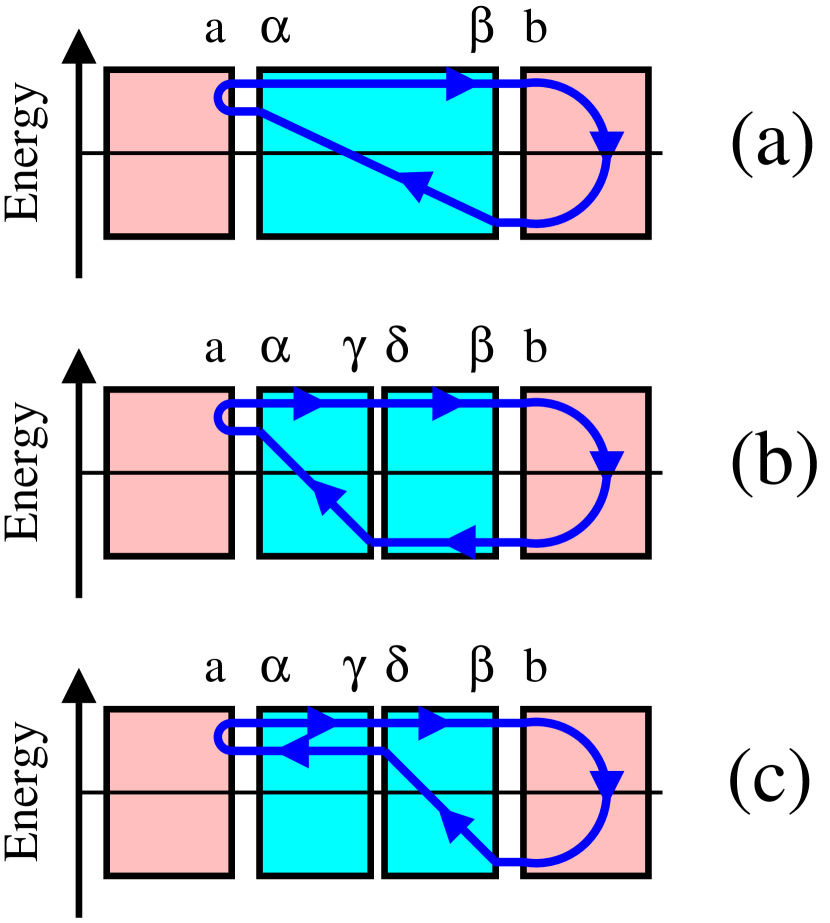
Figure 11: Panel a shows the $\langle\langle g_{(1,1)}g_{(1,2)}\rangle\rangle$ mode at lowest order in the tunnel amplitudes in a $S_{a}IS_{0}IS_{b}$ double junction [${\cal D}^{A,(0)}$ term in Eq. (215)]. Panels b and c show schematically to the ${\cal D}^{A,(1)}$ and ${\cal D}^{A,(2)}$ terms in a $S_{a}IS_{1}IS_{2}IS_{b}$ triple junction, see Eqs. (220)-(221) and Eqs. (222)-(223) respectively.

It is concluded to change of sign in $\langle\langle g_{(1,1)}g_{(1,2)}\rangle\rangle$ connecting $S_{a}$ and $S_{b}$, between the following two situations:

(i) Eq. (225) for ${\cal D}^{A,(0)}$ in a $S_{L}IS_{0}IS_{R}$ double ballistic tunnel junction.

(ii) Eq. (228) for ${\cal D}^{A,(1)}+{\cal D}^{A,(2)}$ in a $S_{a}IS_{1}IS_{2}IS_{b}$ triple ballistic tunnel junction.

This resolves the apparent paradox that emerged between the preceding calculations of the $\langle\langle g_{(1,1)}g_{(1,2)}\rangle\rangle$ mode:

(iii) Eqs. (213)-(214) for $\langle\langle g_{(1,1)}g_{(1,2)}\rangle\rangle$ in the ballistic limit.

(iv) Eqs. (206)-(207) for impurity scattering the $\langle\langle g_{(1,1)}g_{(1,2)}\rangle\rangle$ superconducting diffusion mode at the order $v^{2}$.

Appendix D Details on the calculation of the current-phase relations

D.1 Demonstration of Eq. (73) for $I_{c,\,3TQ_{1}}$

We evaluate the following integral:

$$I_{1}=\int_{-\infty}^{0}\frac{\Delta^{4}}{\left(\Delta^{2}-(\omega-i\eta)^{2}\right)^{2}}d\omega.$$ (229)

We expand according to $\omega-i\eta=-\Delta+\epsilon$. Assuming $|\epsilon|\ll\Delta$ leads to

$$\frac{\Delta^{4}}{\left(\Delta^{2}-(\omega-i\eta)^{2}\right)^{2}}\simeq\frac{\Delta^{2}}{4\epsilon^{2}}+\frac{\Delta}{8\epsilon}+....$$ (230)

If $\eta\ll\Delta$, contour integration yields

$$I_{1}=\frac{i\pi\Delta}{4}.$$ (231)

Eq. (231) is used in subsection V.1 to deduce the quartet current-phase relations Eqs. (71)-(73) from Eq. (70).

D.2 Demonstration of Eq. (86) for $I_{c,\,4TSQ}^{(1)}$

Now, we evaluate

$$I_{2}=\int_{-\infty}^{0}\frac{\Delta^{6}}{\left(\Delta^{2}-(\omega-i\eta)^{2}\right)^{3}}d\omega.$$ (232)

Expanding around $\omega-i\eta=-\Delta+\epsilon$ with $|\epsilon|\ll\Delta$ leads to

$$\frac{\Delta^{6}}{\left(\Delta^{2}-(\omega-i\eta)^{2}\right)^{3}}\simeq\frac{\Delta^{3}}{8\epsilon^{3}}+\frac{3\Delta^{2}}{16\epsilon^{2}}+\frac{3\Delta}{16\epsilon}+...$$ (233)

The residue of the simple pole is $3\Delta/16$. Contour integration yields

$$I_{2}=\frac{3i\pi\Delta}{8}$$ (234)

if $\eta\ll\Delta$. Eq. (234) is used in subsection V.3.1 to deduce the four-terminal 4TSQ current-phase relations Eqs. (85)-(86) from Eq. (84).

D.3 Demonstration of Eq. (92) for $I_{c,\,4TSQ}^{(2)}$

The integral

$$I_{3}=\int_{-\infty}^{0}\frac{(\omega-i\eta)^{2}\Delta^{4}}{\left(\Delta^{2}-(\omega-i\eta)^{2}\right)^{3}}d\omega$$ (235)

is equal to:

$$I_{3}=I_{2}$$ (236)

if $\eta\ll\Delta$, where $I_{2}$ is given by Eq. (234). The leading-order four-terminal 4TSQ current-phase relations Eqs. (91)-(92) are deduced from Eq. (90) by making use of Eqs. (235)-(236), see subsection V.3.2.

D.4 Averaging the product of three superconducting Green’s functions

The average over disorder of the product of three Green’s functions

$${\cal C}_{3}=\langle\langle{g_{(1,1)}g_{(1,2)}g_{(2,2)}}\rangle\rangle$$ (237)

appears in the expression of the four-terminal 4TSQ at the orders $(J_{0}/W)^{12}$ and $\sqrt{{\cal S}_{contact}}/l_{e}$, see Eqs. (9)-(46) in subsection II A of the Supplemental Materialsupplemental .

Each of the three Green’s function appearing in Eq. (237) can propagate locally or nonlocally within the superconducting lead $S_{N}$ having superconducting phase variable $\varphi_{N}$.

The Wick theorem leads to

$${\cal C}_{3} = \langle\langle{g_{(1,1)}g_{(1,2)}}\rangle\rangle\langle\langle g_{(2,2)}\rangle\rangle+\langle\langle{g_{(1,1)}g_{(2,2)}}\rangle\rangle\langle\langle g_{(1,2)}\rangle\rangle$$ (238)

$$+ \langle\langle g_{(1,1)}\rangle\rangle\langle\langle{g_{(1,2)}g_{(2,2)}}\rangle\rangle,$$

where Eqs. (157) and (158) imply the following for the local Green’s functions of the disordered superconductor $S_{N}$:

$$\langle\langle g_{(1,1)}\rangle\rangle = \langle\langle g_{(2,2)}\rangle\rangle=\frac{1}{W}\frac{-(\omega-i\eta)}{\sqrt{|\Delta|^{2}-(\omega-i\eta)^{2}}}$$ (239)

$$\langle\langle g_{(1,2)}\rangle\rangle = =\frac{1}{W}\frac{|\Delta|}{\sqrt{|\Delta|^{2}-(\omega-i\eta)^{2}}}\exp\left(i\varphi_{N}\right).$$ (240)

Combining with the energy dependence of Eq. (205) and Eq. (206) implies the minus sign in

$${\cal C}_{3}\sim-\frac{\Delta^{3}}{W^{2}\left(|\Delta|^{2}-(\omega-i\eta)^{2}\right)^{3/2}}\exp\left(i\varphi_{N}\right),$$ (241)

which is taken into account in the four-terminal 4TSQ critical current at the orders $(J_{0}/W)^{12}$ and $\sqrt{{\cal S}_{contact}}/l_{e}$, see Eq. (86) in the paper and subsection II A in the Supplemental Materialsupplemental .

References

- (1) P. W. Anderson, Random-Phase Approximation in the Theory of Superconductivity, Phys. Rev. 112, 1900 (1958).
- (2) P. W. Anderson, Plasmons, Gauge Invariance, and Mass, Phys. Rev. 130, 439 (1963).
- (3) B.D. Josephson, Possible new effects in superconductive tunnelling, Physics Letters 1, 251 (1962).
- (4) K.F. Huang, Y. Ronen, R. Mélin, D. Feinberg, K. Watanabe, T. Taniguchi and P. Kim, Quartet supercurrent in a multi-terminal Graphene-based Josephson Junction, cond-mat preprint (2020).
- (5) A. Freyn, B. Douçot, D. Feinberg and R. Mélin, Production of non-local quartets and phase-sensitive entanglement in a superconducting beam splitter, Phys. Rev. Lett. 106, 257005 (2011).
- (6) R. Mélin, D. Feinberg and B. Douçot, Partially resummed perturbation theory for multiple Andreev reflections in a short three-terminal Josephson junction, Eur. Phys. J. B 89, 67 (2016).
- (7) T. Jonckheere, J. Rech, T. Martin, B. Douçot, D. Feinberg, and R. Mélin, Multipair DC Josephson resonances in a biased allsuperconducting bijunction, Phys. Rev. B 87, 214501 (2013).
- (8) J. Rech, T. Jonckheere, T. Martin, B. Douçot, D. Feinberg, and R. Mélin, Proposal for the observation of nonlocal multipair production, Phys. Rev. B 90, 075419 (2014).
- (9) R. Mélin, M. Sotto, D. Feinberg, J.-G. Caputo and B. Douçot, Gate-tunable zero-frequency current cross-correlations of the quartet mode in a voltage-biased three-terminal Josephson junction, Phys. Rev. B 93, 115436 (2016).
- (10) R. Mélin, J.-G. Caputo, K. Yang and B. Douçot, Simple Floquet-Wannier-Stark-Andreev viewpoint and emergence of low-energy scales in a voltage-biased three-terminal Josephson junction, Phys. Rev. B 95, 085415 (2017).
- (11) R. Mélin, R. Danneau, K. Yang, J.-G. Caputo, and B. Douçot, Engineering the Floquet spectrum of superconducting multiterminal quantum dots, Phys. Rev. B 100, 035450 (2019).
- (12) B. Douçot, R. Danneau, K. Yang, J.-G. Caputo and R. Mélin, Berry phase in superconducting multiterminal quantum dots, Phys. Rev. B 101, 035411 (2020).
- (13) A. H. Pfeffer, J. E. Duvauchelle, H. Courtois, R. Mélin, D. Feinberg, and F. Lefloch, Subgap structure in the conductance of a three-terminal Josephson junction, Phys. Rev. B 90, 075401 (2014).
- (14) Y. Cohen, Y. Ronen, J.H. Kang, M. Heiblum, D. Feinberg, R. Mélin and H. Strikman, Non-local supercurrent of quartets in a three-terminal Josephson junction, Proc. Natl. Acad. Sci. U. S. A. 115, 6991 (2018).
- (15) J. E. Zimmerman and A. H. Silver, Macroscopic Quantum Interference Effects through Superconducting Point Contacts, Phys. Rev. 141, 367 (1966).
- (16) J.D. Pillet, V. Benzoni, J. Griesmar, J.-L. Smirr and Ç. Ö. Girit, Nonlocal Josephson Effect in Andreev Molecules Nano Lett. 19, 7138 (2019).
- (17) J.-D. Pillet, V. Benzoni, J. Griesmar, J.-L. Smirr and Ç Ö Girit, Scattering description of Andreev molecules, SciPost Phys. Core 2, 009 (2020).
- (18) R.-P. Riwar, M. Houzet, J.S. Meyer, and Y.V. Nazarov, Multi-terminal Josephson junctions as topological materials, Nat. Commun. 7, 11167 (2016).
- (19) E. Eriksson, R.-P. Riwar, M. Houzet, J. S. Meyer, and Y. V. Nazarov, Topological transconductance quantization in a four-terminal Josephson junction, Phys. Rev. B 95, 075417 (2017).
- (20) E. Strambini, S. D’Ambrosio, F. Vischi, F.S. Bergeret, Yu.V. Nazarov, and F. Giazotto, The -SQUIPT as a tool to phase-engineer Josephson topological materials, Nat. Nanotechnol. 11, 1055 (2016).
- (21) A.W. Draelos, M.-T. Wei, A. Seredinski, H. Li, Y. Mehta, K. Watanabe, T. Taniguchi, I.V. Borzenets, F. Amet, and G. Finkelstein, Supercurrent flow in multiterminal graphene Josephson junctions, Nano Lett. 19, 1039 (2019).
- (22) N. Pankratova, H. Lee, R. Kuzmin, K. Wickramasinghe, W. Mayer, J. Yuan, M.G. Vavilov, J. Shabani, and V.E. Manucharyan, Multi-terminal Josephson effect, Phys. Rev. X 10, 031051 (2020).
- (23) G. Falci, D. Feinberg F.W.J. Hekking, Correlated tunneling into a superconductor in a multiprobe hybrid structure, Europhys. Lett. 54, 255 (2001).
- (24) R. Mélin and D. Feinberg, Sign of the crossed conductances at a ferromagnet/superconductor/ferromagnet double interface, Phys. Rev. B 70, 174509 (2004).
- (25) G. Deutscher and D. Feinberg, Coupling superconducting-ferromagnetic point contacts by Andreev reflections, Appl. Phys. Lett. 76, 487 (2000).
- (26) T. H. Stoof and Yu. V. Nazarov, Flux effect in superconducting hybrid Aharonov-Bohm rings, Phys. Rev. B 54, R772(R) (1996).
- (27) See the Supplemental Material which contains technical details of the calculations.
- (28) S. B. Kaplan, C. C. Chi, D. N. Langenberg, J. J. Chang, S. Jafarey, and D. J. Scalapino, Quasiparticle and phonon lifetimes in superconductors, Phys. Rev. B 14, 4854 (1976).
- (29) R. C. Dynes, V. Narayanamurti, and J. P. Garno, Direct measurement of quasiparticle-lifetime broadening in a strong-coupled superconductor, Phys. Rev. Lett. 41, 1509 (1978);
- (30) J.P. Pekola, V. F. Maisi, S. Kafanov, N. Chekurov, A. Kemppinen, Yu. A. Pashkin, O.-P. Saira, M. Möttönen, and J. S. Tsai, Environment-assisted tunneling as an origin of the Dynes density of states, Phys. Rev. Lett. 105, 026803 (2010).
- (31) O.-P. Saira, A. Kemppinen, V. F. Maisi, and J. P. Pekola, Vanishing quasiparticle density in a hybrid Al/Cu/Al single-electron transistor, Phys. Rev. B 85, 012504 (2012).
- (32) C. Caroli, R. Combescot, P. Nozières and D. Saint-James, Direct calculation of the tunneling current, Jour. Phys. C: Solid State Phys. 4, 916 (1971).
- (33) J. C. Cuevas, A. Martín-Rodero, and A. Levy Yeyati, Hamiltonian approach to the transport properties of superconducting quantum point contacts, Phys. Rev. B 54, 7366 (1996).
- (34) A.A. Abrikosov, L.P. Gorkov and I.E. Dzyaloshinski, Methods of Quantum Field Theory in Statistical Physics, Prentice Hall, 1st Edition 1963.
- (35) R.A. Smith and V. Ambegaokar, Weak-localization correction to the number density of superconducting electrons, Phys. Rev. B 45, 2463 (1992)
- (36) D. Gosselin, G. Hornecker, R. Mélin and D. Feinberg, Phase-sensitive transport at a normal metal–superconductor interface close to a Josephson junction, Phys. Rev. B 89, 075415 (2014).
- (37) R. Mélin, Contribution of weak localization to nonlocal transport at normal metal/superconductor double interfaces, Phys. Rev. B 73, 174512 (2006).
- (38) M. Wampler, P. Schauss, E. B. Kolomeisky, and I. Klich, Quantum wakes in lattice fermions, arXiv: 2006.094669v1 (2020).
- (39) W. Guichard, M. Aprili, O. Bourgeois, T. Kontos, J. Lesueur, and P. Gandit, Phase Sensitive Experiments in Ferromagnetic-Based Josephson Junctions,Phys. Rev. Lett. 90, 167001 (2003).
- (40) M. A. H. Nerenberg, J. A. Blackburn, and D. W. Jillie, Voltage locking and other interactions in coupled superconducting weak links. I. Theory, Phys. Rev. B 21, 118 (1980).
- (41) D. W. Jillie, M. A. H. Nerenberg, and J. A. Blackburn, Voltage locking and other interactions in coupled superconducting weak links. II. Experiment, Phys. Rev. B 21, 125 (1980).
- (42) A. Levy Yeyati, F.S. Bergeret, A. Martín-Rodero and T.M. Klapwijk, Entangled Andreev pairs and collective excitations in nanoscale superconductors, Nature Phys. 3, 455 (2007).
- (43) G.E. Blonder, M. Tinkham and T.M. Klapwijk, Transition from metallic to tunneling regimes in superconducting microconstrictions: Excess current, charge imbalance, and supercurrent conversion, Phys. Rev. B 25, 4514 (1982).
- (44) M. Flöser, D. Feinberg and R. Mélin, Absence of split pairs in the cross-correlations of a highly transparent normal metal-superconductor-normal metal electron beam splitter, Phys. Rev. B 88, 094517 (2013).