A SOFIA Survey of [C ii] in the galaxy M51 II. [C ii] and CO kinematics across spiral arms

Abstract

We present the first complete, velocity–resolved [C ii] 158$\mu$m image of the M51 grand-design spiral galaxy, observed with the upGREAT instrument on SOFIA. [C ii] is an important tracer of various phases of the interstellar medium (ISM), including ionized gas, neutral atomic, and diffuse molecular regions. We combine the [C ii] data with H i, CO, 24$\mu$m dust continuum, FUV, and near–infrared K–band observations to study the evolution of the ISM across M51’s spiral arms in both position–position, and position–velocity space. Our data show strong velocity gradients in H i, ¹²CO, and [C ii] at the locations of stellar arms (traced by K–band data) with a clear offset in position–velocity space between upstream molecular gas (traced by ¹²CO) and downstream star formation (traced by [C ii]). We compare the observed position–velocity maps across spiral arms with synthetic observations from numerical simulations of galaxies with both dynamical and quasi–stationary steady spiral arms that predict both tangential and radial velocities at the location of spiral arms. We find that our observations, based on the observed velocity gradients and associated offset between CO and [C ii], are consistent with the presence of shocks in spiral arms in the inner parts of M51 and in the arm connecting the companion galaxy, M51b, in the outer parts of M51.

1 Introduction

The cycling of the interstellar medium (ISM) through different phases, including the eventual formation of stars in gravitationally bound regions, is the driving agent in the evolution of galaxies. The standard picture of the phases of the ISM in spiral galaxies posits that Giant Molecular Clouds (GMCs) are assembled in the spiral arm shocks from diffuse inter-arm H i gas, and then photo–dissociated back into the atomic phase by OB star formation within the spiral arms (Binney & Merrifield, 1998). This picture predicts a rapid phase change of gas across spiral arms–from the atomic to molecular and back into atomic–synchronized by spiral arm forcing (Klessen & Glover, 2016). On the other hand, CO imaging of M51 shows much less gas-phase variation across the spiral arms (Koda et al., 2009); the majority of the ISM gas remains molecular through the interarm regions, surviving to the next spiral arm passage. These observations are consistent with numerical simulations of galactic disks, in which a large reservoir of molecular gas is predicted to exist in the inter–arm region of galaxies (Smith et al., 2014; Duarte-Cabral et al., 2015).

To understand galactic disks, we need to gain a full understanding of spiral structure – the interrelation between all the gaseous and stellar components, and their connection to the star formation process. Although we can separate the different stellar populations, measure kinematics, and study much of the ISM on a cloud–by–cloud basis with optical, H i and CO observations, we do not have the same information on the diffuse atomic, atomic–molecular transition (Wannier et al., 1991), and warm ionized components of the interstellar medium. These components are traced by the [C ii] 158$\mu$m line, which only now can be observed with the velocity resolution required to understand its link to the other phases. [C ii] traces the diffuse ionized medium, warm and cold atomic clouds, clouds in transition from atomic to molecular, and dense and warm photon dominated regions (PDRs). In particular, this line is a tracer of the CO–dark H₂ gas (Grenier et al., 2005; Wolfire et al., 2010; Langer et al., 2010) which is likely a precursor of the dense molecular gas that will eventually form stars.

In this paper we present the first complete, velocity resolved [C ii] 158$\mu$m map of the M51 grand-design spiral galaxy, observed using the upgraded German REceiver for Astronomy at Terahertz frequencies (upGREAT) instrument on the Stratospheric Observatory For Infrared Astronomy (SOFIA). This map was obtained as part of a Joint Impact Proposal (program ID 04_0116) that also includes a velocity unresolved [C ii] map of M51 obtained with the Far Infrared Field-Imaging Line Spectrometer (FIFI-LS) instrument on SOFIA, and presented in Pineda et al. (2018). M51 is a nearby grand design spiral at 8.6 Mpc (McQuinn et al., 2016) with a low inclination angle of 24° (Daigle et al., 2006). It has been extensively studied in many tracers, including CO (Aalto et al., 1999; Koda et al., 2009; Schinnerer et al., 2013; Miyamoto et al., 2014), H i (Walter et al., 2008), optical light (Mutchler et al., 2005), radio continuum (Fletcher et al., 2011; Querejeta et al., 2019), dust continuum (Mentuch Cooper et al., 2012), and dense gas tracers (Bigiel et al., 2016). These observations have allowed the spatial separation of different ISM constituents, including Hii regions, OB stars, and atomic and molecular clouds. Partial maps of M51 in [C ii], at low spectral resolution, have been presented by Nikola et al. (2001) and Parkin et al. (2013). Our complete [C ii] map in M51 allows us to trace the ISM phases probing atomic, PDR, and CO–dark H₂ gas over the entire disk, including both arm and inter-arm regions at high spectral resolution.

In spiral galaxies, spiral density waves play a fundamental role assembling the giant molecular clouds in which star formation takes place. There are two competing theories of the nature of spiral arms in isolated galaxies. In the quasi–stationary spiral structure (QSSS) hypothesis, spiral arms are thought to be rigidly rotating, long–lived patterns that persist over several galactic rotations (see Bertin & Lin 1996 for a review). The spiral density wave affects the gas flow, resulting in shocks around spiral arms, triggering phase transitions in the ISM. Alternatively, the transient spiral hypothesis (Goldreich & Lynden-Bell, 1965; D’Onghia et al., 2013; Baba et al., 2013; Dobbs & Baba, 2014) suggests that each spiral arm is a transient feature generated by the swing-amplification mechanism. Its amplitude varies on the timescale of epicyclic motions (a fraction of galactic rotation timescale). In this theory, the gas flows toward the potential minimum of the spiral arm from both sides of the arm. This model is in contrast to the gas passage from one side of the spiral arm to the other predicted in the density wave model. Determining the nature of spiral arms is a fundamental aspect in the understanding of the evolution of spiral galaxies.

Several observational methods have been applied to distinguish between different theories of the nature of spiral arms in M51, including searches for offsets across spiral arms between stellar cluster with different ages (Dobbs & Pringle, 2010; Shabani et al., 2018; Chandar et al., 2017) and between images of different ISM and star formation tracers (Tamburro et al., 2008; Foyle et al., 2011; Louie et al., 2013; Egusa et al., 2017). These methods, however, often provide contradicting results. It has been recently proposed that the kinematic information of gas tracers in spirals provides an important tool for distinguishing between these two spiral structure theories (Baba et al., 2016). Because spiral arms dynamically affect the flow of gas, they also affect the structure of the interstellar medium. Thus, having a complete picture of the ISM phases with high spectral resolution observations over large areas in galaxies is a fundamental requirement for determining the nature and effects of spiral arms in disk galaxies. The grand–design spiral structure in M51 is thought to be caused by the tidal interaction between its companion galaxy M51b (Toomre & Toomre, 1972; Pettitt et al., 2017; Tress et al., 2019). M51 is therefore an excellent laboratory for studying the nature of spiral arms, and how they affect the evolution of the ISM and star formation.

This paper is organized as follows. In Section 2, we describe the [C ii] observations and the ancillary data used to study the evolution of the ISM in M51’s spirals. In Section 3, we describe techniques used to remove the rotation velocity of the galaxy and mask the galaxy so that data can be combined to amplify the signal produced by gas velocity variations due to the presence of spiral density waves. In Section 4, we study the spatial (2D) distribution of the different ISM traces across spiral arms (Section 4.1) and we investigate the distribution of ISM phases in the position–velocity space (Section 4.2), including a comparison between observations and predictions from QSSS and transient spiral hypothesis model–predicted position–velocity maps (Section 4.2.1). We summarize our results in Section 5.

2 Observations

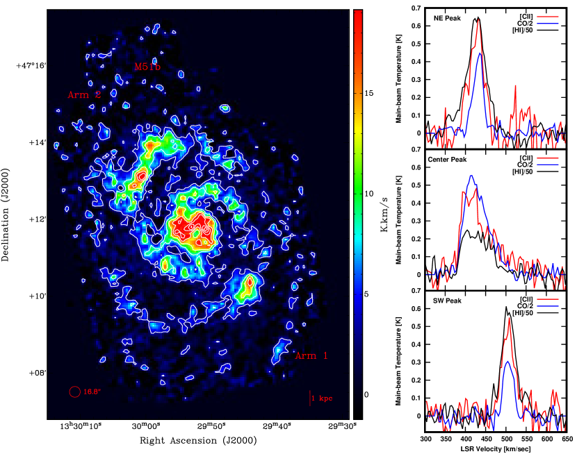
Figure 1: (left) [C ii] integrated intensity map of M51 observed with the upGREAT instrument on SOFIA, having an angular resolution of 16.8″, corresponding of 700 pc for a distance to M51 of 8.6 Mpc. The contours range from 31% to 91% of the peak integrated intensity (19.1 K km s^-1) in steps of 10%. We denote the location companion galaxy, M51b, in the northern part of the map. (right) Sample [C ii], CO, and H i spectra corresponding to the [C ii] peaks at the north–east, central, and south–west regions in M51.

2.1 upGREAT Observations

We observed the [C ii] ²P${}_{3/2}-^{2}$P_1/2 fine–structure line at 1900.5469 THz (rest frequency) in M51 with the upGREAT (Risacher et al., 2016) instrument on the Stratospheric Observatory for Far–Infrared Astronomy (SOFIA; Young et al. 2012). We covered an area of 6′$\times$12′, extending over the full extent of M51 and its companion M51b. The upGREAT instrument uses a $2\times 7$–pixel sub–arrays in orthogonal polarization, each in an hexagonal array around a central pixel. We employed an optimized on–the–fly (OTF) mapping scheme in which the array is rotated by 19.1° and a vertical and a horizontal scan are undertaken. This results in a fully–sampled 73″$\times$73″ square region (tile). To cover the full extent of M51 we observed 34 such tiles. For baseline stability we used chopped–OTF mapping mode with two reference positions located to the east (13:29:13.5, 47:07:32.9; J2000) and west (13:29:31.9, 47:09:12.9; J2000) sides of M51. The angular resolution of the [C ii] observations is 16.8″, corresponding to 700 pc for a distance to M51 of 8.6 Mpc. In our analysis, we deprojected the [C ii] cube, and all other data cubes and images described below, assuming the center, inclination, and position angle listed in Table 1.

We processed the data using the CLASS90 data analysis software. We fitted polynomial baselines (typically of order 3), smoothed the data in velocity, and resampled the data into a regular spatial grid. We also apply a set of main–beam efficiencies that are appropriate to each pixel of the upGREAT array to transform the data from antenna temperature to main–beam temperature scale. The average main–beam efficiency is 0.68 (Risacher et al., 2016). The typical rms noise of the resulting data is 0.06 K in a 3.8 km s^-1 channel width. We compared the integrated intensities of our upGREAT [C ii] map with those observed in the inner parts of M51 with Herschel/PACS (Parkin et al., 2013), smoothed to a 16.8″ angular resolution, and with the FIFI–LS [C ii] map presented in Pineda et al. (2018). We find good agreement in the integrated intensities between these three maps with differences within the uncertainties of the observations. The integrated intensity map of M51 observed with the upGREAT instrument is shown in the left panel of Figure 1. The [C ii] distribution in M51 is characterized by bright emission in its central region, with the [C ii] peak being about 22.5″ or 900 pc from M51’s center, and in two regions at about 5.3 kpc from the galaxy’s center. In the right panel of Figure 1, we show the velocity–resolved [C ii], ¹²CO, and H i spectra corresponding to the [C ii] peaks at the north–east, central, and south–west regions. We see that the line [C ii] widths are typically broader than those of CO, but somewhat narrower compared with those of H i. The companion galaxy, M51b, which is located at the northern portion of the map, is not detected in our upGREAT map, but it is detected in our FIFI–LS map. A comparison between H$\alpha$ and mid– and far–infrared tracers and [C ii] is discussed in Pineda et al. (2018).

2.2 H i and CO Observations

In our analysis we employed the H i spectral cube obtained in M51 using the VLA as part of the THINGS project (Walter et al., 2008). The data has been produced with a robust weighting scheme and has an angular resolution of $\sim$6″. We smoothed the data to 16.8″ and regridded the H i data to that of the [C ii] map for comparison. Note that these interferometric observations lack short spacing data. However, these observations are sensitive to scales up to $\sim$15′, greater than the full extent of M51. Additionally, the total H i flux of M51 observed with the VLA is consistent with previous, lower resolution, single–dish observations (see Table 5 in Walter et al., 2008). The rms noise of the H i data is 0.3 K in a 3.8 km s^-1 channel width.

We used the ¹²CO $J=1\to 0$ map observed with the CARMA interferometer, with data for a short spacing correction obtained with the Nobeyama Radio Observatory 45 telescope (Koda et al., 2009). We smoothed and regrided the ¹²CO map, from its original resolution of 4″, to match the 16.8″ resolution of the [C ii] data cube. The resulting ¹²CO maps has a rms noise of 0.07 K in a 3.8 km s^-1 wide channel. We also employed the ¹²CO and ¹³CO $J=1\to 0$ cubes observed with the IRAM 30 m telescope presented by Pety et al. (2013), as they better sample regions in the outer portions of M51. The angular resolution of the ¹²CO and ¹³CO cubes is 22.5″ and the rms noise is 0.016 K in a 5 km s^-1 wide channel.

2.3 24$\mu$m continuum, FUV, and K–band near-IR Maps

We also compared our [C ii] dataset with 24$\mu$m, FUV maps, and K–band optical maps, tracing warm dust, evolved unobscured star formation, and stellar mass, respectively. The 24$\mu$m continuum map was observed as part of the Spitzer/SAGE survey (Kennicutt et al., 2003) and has a native angular resolution of 6″. The FUV image was obtained by the GALEX satellite and presented by Gil de Paz et al. (2007) with a native resolution of 4.2″. The K–band near–infrared data was observed by 2MASS and presented by Jarrett et al. (2003) with a native resolution of 2.5″. All maps were smoothed with a Gaussian kernel and regridded to match the 16.8″ angular resolution and positions of our [C ii] observations.

3 Gridding, Masking, and Derotation

3.1 Spatial Gridding

Table 1: Adopted Parameters of M51

Parameter	Value
R.A. (J2000)	13:29:52.771
Decl. (J2000)	+47:11:42.62
P.A.1	169.0$\pm$4.2°
Incl.2	24$\pm$3°
Distance	8.6 Mpc

In the following sections we discuss the distribution of different ISM and star formation tracers across the spiral arms of M51 in both spatial and spatial–velocity space. In order to allow the comparison with continuum tracers (FUV, K–band NIR, etc), we first studied the CO and [C ii] integrated intensities in our analysis. We use the azimuthal distribution of these intensities to investigate possible shifts in their peak intensity that would result from the presence of spiral density waves. Such azimuthal intensity distributions are often averaged in a set of annuli with a given radial width with the aim of improving the signal–to–noise ratio of the observations. However, within such annuli, the spiral arm structure varies rapidly with radius, and averaging in the radial direction results in confusion between arm and inter–arm regions. To facilitate the separation between arm and inter–arm regions, following Koda et al. (2012), we defined a set of spiral arm segments that follow the spiral structure of M51. Such segments ensure that the averaging is done in arms and inter–arm regions separately. The spiral structure of a galaxy can be characterized by logarithmic spirals given as,

$$\theta=\frac{-1}{\tan(i_{\rm pitch})}\ln(r)+\theta_{0},$$ (1)

where $\theta$ is the azimuthal angle, $r$ the radius, and $i_{\rm pitch}$ the pitch angle, and $\theta_{0}$ is the phase angle. The origin of azimuthal angle starts at the west part of the map and increases clockwise. The azimuthal angle is the counterclockwise angle from the positive x-axis (west) in the map. The entire extent of M51 cannot be described by a single pitch angle, as changes in this angle are apparent in the two [C ii] bright regions about 127″ (5.3 kpc) from the center, and at the outer spiral arms. We therefore define four regions that are characterized by different values of $i_{\rm pitch}$: M51’s inner galaxy, middle north, middle south, and Outer galaxy. The radial limits and pitch angles of these regions are listed in Table 2. For the inner galaxy, we adopted the pitch angle used by Koda et al. (2012), but for the middle and outer masks we adopted pitch angles that approximately match the observed spiral pattern. We tested whether small variations ($\pm$10%) in the assumed pitch angles affect the resulting spatial and spatial–velocity distributions studied below and found that they are not significantly affected.

We construct a grid of spiral segments over M51 that are parameterized by the phase angle $\theta_{0}$ in Equation (1). We scale the values of $\theta_{0}$ in each mask to range between 0 and 2$\pi$, and we rotate the origin of the phase angle distribution so that it follows the spiral pattern. This rotation results in the spiral arms being at about the same phase angle at any radius. In Figure 2 we illustrate our definition of the spiral arm segments used in our analysis over the 24 $\mu$m dust continuum image of M51. In the upper left panel, we show the radial mask, which corresponds to rings of $\sim 1$ kpc width extending from 1.5 kpc and 9.1 kpc. In the upper right panel, we show the definition of the Inner, Middle North, Middle South, and outer regions which are characterized by different pitch angles (Table 2). In the lower left panel, we show the spiral grid, which is defined by 32 segments with a step in $\theta_{0}$ of 0.098 radians. We highlight in black the spiral segments at the location of the spirals in the 24 $\mu$m image. The thick white lines are artifacts of the contouring that becomes thicker when there are discontinuities in the phase angle distribution. Such discontinuities are either produced at the origin of the phase angle distribution, $\theta_{0}=0$ rad, or at the middle masks where spiral arms are close to each other due to the change in the pitch angle. The thicker white line that denotes the origin of the phase angle distribution at each radius follows Arm 2 in the counterclockwise side. Finally, in the lower left panel we show the combined radial and spiral masks in M51.

We show a detailed view of the spiral segments in Figure 3. The spiral segments shown in the figure correspond to Ring 2, which extends between 2.6 kpc and 3.6 kpc from M51’s center. The integrated intensity and position–velocity distribution discussed in Section 4.2 are the result of the data averaged within each spiral segments in the figure. The thick white line at the bottom represents the origin, $\theta_{0}=0$ rad, of the phase angle distribution which increases counterclockwise. This method has the advantage that it does not depend on any specific definition of a spiral arm in the image data and ensures that emission in arm and inter-arm regions are not averaged together.

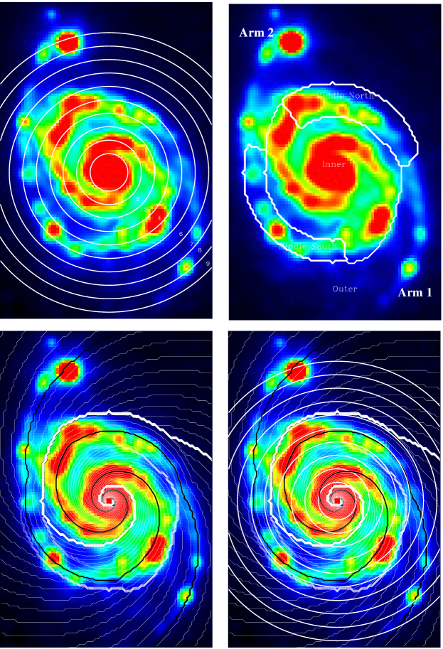
Figure 2: (top left) Azimuthal rings displayed over the 24$\mu$m continuum emission image of M51. The rings extend from 1.5 kpc to 9.1 kpc, in steps of $\sim$1 kpc. (top right) Definition of the regions that are characterized by different values of the pitch angle (see Table 2) that are used to create the spiral pattern grid. (bottom left) Logarithmic spiral pattern definition overlaid on the 24$\mu$m continuum emission image of M51 (see Section 3). The black lines show the spiral pattern at the location of the spiral arms and the thick white line counterclockwise of Arm 2 represents the origin, $\theta_{0}=0$ rad, of the phase angle distribution. (bottom right) The combined azimuthal and spiral mask that defines the segments from which we derive averaged intensities and the stacked spectra used in our analysis.

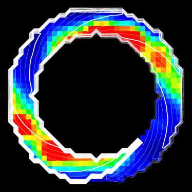
Figure 3: Definition of spiral segments for a ring between 2.6 kpc and 3.6 kpc from M51’s center, overlaid over the 24 $\mu$m dust continuum image on M51. The thick white line at the bottom represents the origin, $\theta_{0}=0$ rad, of the phase angle distribution which increases anti-clockwise.

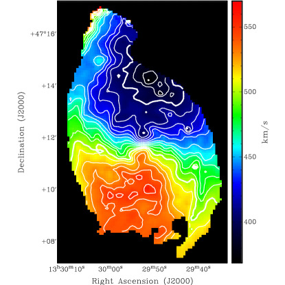
Figure 4: Mass–weighted velocity centroid distribution in the disk of M51 derived from H i and ¹²CO maps. Contours range from 360 to 570 km s^-1 in steps of 10 km s^-1.

Table 2: Definition of Regions in M51

Region	$R^{1}_{\rm in}$	$R^{1}_{\rm out}$	$\Phi^{2}_{\rm in}$	$\Phi^{2}_{\rm out}$	$i^{3}_{\rm pitch}$
Inner4	0″	160″	0	2$\pi$	18.5°
Middle North5	106″	180″	0	0.7$\pi$	2°
Middle South5	132″	191″	0.95$\pi$	1.55$\pi$	2°
Outer4	160″	300″	0	2$\pi$	28°

Figure 5: ¹²CO (left), [C ii] (center), and FUV (right) images of M51. The ¹²CO, [C ii], and FUV maps trace cold gas, warm and dense PDRs, and evolved unobscured star forming regions, respectively.

3.2 Velocity Derotation

Spiral density waves not only can result in different spatial distributions of CO, H i, [C ii], and other tracers, but they also imprint a particular velocity distribution on the gas (Roberts & Stewart, 1987; Baba et al., 2016). These velocity features, if related to the compression of gas caused by shocks, are likely associated with the transition between ISM phases, and therefore variations in the position–velocity distribution of CO, H i, and [C ii] are expected.

The observed velocity of spectral lines in the galaxy is a combination of M51’s systemic velocity, the rotational velocity, and peculiar (related to the spiral perturbation) velocities (see e.g. Shetty et al., 2007). With the aim to study how the position–velocity distribution of H i, CO, and [C ii] intensities is affected by spiral density waves, we need to isolate velocity variations due to spiral density waves from those due to the systemic and rotation velocity of the galaxy. To do so, we define a reference velocity frame that co–rotates with the spiral density perturbation. Assuming that the gas mass peaks in an area associated with the location of the spiral density perturbation, we define the velocity at which most of the mass rotates to be the reference velocity frame. We start by estimating the total hydrogen surface density per velocity bin at each voxel in a position–velocity data cube of M51. We generate a total hydrogen surface density per unit velocity, $\sigma_{\rm H}=\sigma_{\rm H^{0}}+\sigma_{\rm H_{2}}$, cube by combining the H i and ¹²CO $J=1\to 0$ data cubes. The neutral atomic, H⁰, and molecular, H₂, hydrogen surface densities per velocity bin are given by,

$$\sigma_{\rm H^{0}}=\Sigma_{\rm H^{0}}/\Delta v,$$ (2)

and

$$\sigma_{\rm H_{2}}=\Sigma_{\rm H_{2}}/\Delta v,$$ (3)

respectively, where $\Sigma_{\rm H^{0}}$ and $\Sigma_{\rm H_{2}}$ are the H⁰ and H₂, surface densities, in units of M_⊙ pc^-2, which are in turn given by,

$$\Sigma_{\rm H^{0}}=0.002I_{\rm HI}=0.002T_{\rm HI}\Delta v,$$ (4)

and

$$\Sigma_{\rm H_{2}}=4.37I_{\rm CO}=4.37T_{\rm CO}\Delta v,$$ (5)

where $I_{\rm HI}$ and $I_{\rm CO}$, are the H i and CO integrated intensities in units of K km s^-1, and $T_{\rm HI}$ and $T_{\rm CO}$ intensities at a given velocity channel in units of K. Note that a $\cos(i)$ factor, where $i$ is the galaxy’s inclination (Table I), needed to correct the surface brightness is applied during the deprojection step. The surface density calculation includes a factor of 1.36 to account for heavy elements and the H₂ surface density calculation assumes a $X_{\rm CO}=2\times 10^{20}$ cm^-2(K km s^-1)^-1 (Bolatto et al., 2013). We calculate the mass–weighted velocity centroid in each spatial pixel of the data cube using,

$$V_{\rm cen}=\frac{\sum_{i}^{N}\sigma^{i}_{\rm H}V^{i}_{\rm H}}{\sum_{i}^{N}\sigma^{i}_{\rm H}},$$ (6)

over N channels in each spectra. The uncertainties in the resulting velocity centroids are mostly related to rms noise in the spectra and the presence of noise peaks across the velocity band. We minimize these effects in the derived mass–weighted velocity centroid map by using a diluted mask technique, in which the data cube is smoothed to a lower resolution, so that noise of the spectra is reduced by a factor of $\sim$3. We then create a position–position–velocity mask in which intensities are larger than 4 times the rms noise of the smoothed cube, and applied it to the unsmoothed data cube. The resulting mass–weighted velocity centroid map is shown in Figure 4.

We use the total hydrogen mass–weighted velocity centroid map to shift the velocity axis of the H i, CO, and [C ii] spectra so that the velocity corresponding to $V_{\rm cen}$ becomes zero. This results in data cubes that peak around $V=0$ km s^-1, but show deviations of about $\pm$30 km s^-1. Because these velocity deviations are relative to the velocity of the total hydrogen intensity peak, in a given spectra, the relative differences between the [C ii], H i, and ¹²CO line emission are not sensitive to the exact value of the systemic and rotational components. The de–rotated data cubes will be used in Section 4.2 to study the distribution of H i, CO, and [C ii] across spiral arms.

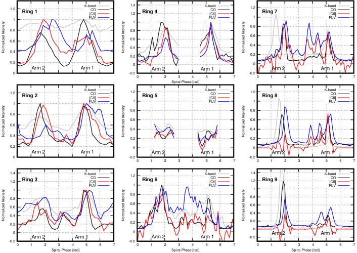
Figure 6: [C ii], ¹²CO, FUV, and K–band NIR infrared intensities as a function of spiral phase. Each panel represent a ring with $\sim$1 kpc width extending from 1.5 kpc to 9.1 kpc (see Figure 2).

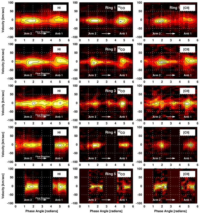
Figure 7: H i, ¹²CO, [C ii] position velocity maps as a function of phase angle. Each panel corresponds to a $\sim$1 kpc radial segment extending from 1.5 kpc to 6.9 kpc.

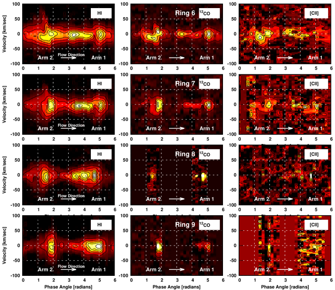
Figure 8: H i, ¹²CO, [C ii] position velocity maps as a function of phase angle. Each panel corresponds to a $\sim$1 kpc radial segment extending from 6.9 kpc to 11.2 kpc.

4 Discussion

4.1 Integrated Intensity Distribution across Spiral Arms

The integrated intensity distribution of different tracers as a function of azimuthal angle for a set of different annuli in galaxies has been used to study the evolution of the ISM in spiral arms and to test theories of spiral structure (Tamburro et al., 2008; Foyle et al., 2011; Egusa et al., 2017). The quasi–stationary spiral arm structure (QSSS) theory predicts that, inside the co-rotation radius, the location of gaseous spiral arms move from upstream to downstream of stellar arms with an offset that decreases as the radius increases. Beyond the co-rotation radius the gaseous arms move from upstream to downstream with the offset increasing with radius (Gittins & Clarke, 2004). Egusa et al. (2017) find that in the inner M51, one arm (Arm 2; see Figure 1) shows offsets between CO and H$\alpha$ emission that are radially ordered between the stellar and gas arms, while the other (Arm 1) does not. Additionally, offsets are not clearly seen in the outer regions of M51. They conclude that the nature of two inner spiral arms in M51 is different than of the outer arms, due to the interaction with the companion galaxy, M51b. Foyle et al. (2011) studied spatial offsets between different ISM and star formation tracers in a sample of 12 galaxies (including M51) using the cross–correlation method (Tamburro et al., 2008; Dobbs et al., 2010). They find no systematic offset variation with radius in any galaxy in their sample and conclude that their observations are inconsistent with the QSSS theory. With the aim at resolving the discrepancies between the studies mentioned above, Louie et al. (2013) studied different methods for determining offsets between gas spiral arm and star formation tracers. They argue that offsets are highly dependent on which gas tracer is used (e.g. CO or H i) and that different methods for measuring the location of spiral arms (Gaussian fitting, cross–correlation) can give discrepant results. They find mostly positive offsets between CO and H$\alpha$, suggesting that gas flow through spiral arms (i.e., density wave), although the spiral pattern may not necessarily be stationary for a timescale much longer than the arm-crossing timescale.

[C ii] provides an unobscured view of the far–ultraviolet illuminated regions associated with massive star formation (Pineda et al., 2018). These observations can be combined with those of low–$J$ transitions of CO, which traces cold and moderately dense molecular gas, and FUV, describing evolved regions in which star formation disrupted their progenitor molecular gas, to study the evolution of the interstellar medium across spiral arms.

In Figure 5, we show our [C ii] map, together with those of ¹²CO and the far–ultraviolet intensity. We see a morphological evolution between ¹²CO, [C ii], and FUV, not only represented as apparent offsets along the flow direction (counterclockwise), but also in terms of small scale structure, with CO being more ordered, while [C ii] and FUV are more non-uniformly distributed. This difference is possibly a result of [C ii] and FUV tracing more energetic environments compared with ¹²CO.

We present a more detailed view of the distribution of different tracers across spiral arms in M51 in Figure 6. We show the normalized integrated intensity of ¹²CO, [C ii], and FUV as a function of the phase angle for a set of rings (Rings 1 to 9; see Figure 2) extending from 1.5 kpc to 9.1 kpc, in steps of $\sim$1 kpc. We also include near–infrared K band observations which trace the stellar mass, and thus the location of bottom of the gravitational potential (Mentuch Cooper et al., 2012). In the inner galaxy (Rings 1–5), we use data at 16.8″ resolution, with the ¹²CO map presented by Koda et al. (2009), while for the outer galaxy (Rings 6–9) we take data smoothed to 23″, corresponding to the angular resolution of the ¹²CO map presented by Pety et al. (2013). This data cube has better coverage and signal–to–noise ratio in the outer regions of M51. We mask out from these figures the galactic center and companion galaxy, M51b, using the mask presented by Pineda et al. (2018). Because of the sudden reduction of the spiral arms pitch angle in the region between 4.75 kpc and 6.9 kpc (Rings 4 and 5), the inter-arm area in this region is greatly reduced and our spiral grid corresponding to these inter-arm regions is truncated. This results in the gaps seen in Figure 6 and Figure 7 for these regions. We see peaks that correspond to the two spiral arms with the direction of the flow being left to right. Following Egusa et al. (2017), we define the arm on the left, connecting to the companion galaxy M51b, as Arm 2 and that on the right, pointing away from the companion, as Arm 1 (see Figure 1).

In the inner M51 (Rings 1 to 3 in Figure 6), there is a clear offset between the peaks of ¹²CO, [C ii], and FUV for Arm 2, but that is not as pronounced in Arm 1, in particular between ¹²CO and [C ii]. The [C ii] and FUV profiles, however, show more extended emission in the direction of the flow compared with CO for both arms. The missing offset between in the intensity peaks in Arm 1 is consistent with that seen by Egusa et al. (2017) but, as we will see in Section 4.2, it is likely the result of using integrated intensities lacking spectral information. The stellar arms traced by NIR K–band emission are typically associated with the gas peaks, but there is no significant offset between them. In the middle region of M51 (Rings 4 and 5), where the pitch angle of spiral arms is significantly reduced, we can still see an offset between ¹²CO, [C ii], and FUV. In the outer galaxy, (Rings 6 to 9) the offsets appear to be smaller. Note that the peak in NIR K–band in Ring 9 for Arm 2 is associated with emission from the companion galaxy that is outside M51b’ mask.

In Rings 6–8 (see also Figure 11), we see emission peaks in the inter–arm regions that are prominent in [C ii] and FUV, but are relatively faint in CO emission. These peaks correspond to arm–like structures in the inter–arm regions in the southern part of M51. The large [C ii]/¹²CO ratio (in units of K km s^-1) is suggestive of the presence of CO–dark H₂ gas in the region (Pineda et al., 2013). A quantitative study of the inter-arm [C ii] in M51 will be presented in a subsequent publication in this series.

Due to the 700 pc spatial resolution of our observations, insufficient for resolving spiral arms spatially, we are unable to confirm whether there is a systematic variation in the offsets between NIR K–band, ¹²CO, [C ii], and FUV as a function of radius. We can, however, use the high spectral resolution of our observations to study the nature of spiral arms in M51, as discussed in the following Section.

4.2 Velocity Distribution across Spiral Arms

The two proposed theories of spiral arm formation discussed above make different predictions about the velocity field of the gas encountering a spiral arm. In the QSSS hypothesis the gas velocity changes suddenly as it approaches the spiral arm, while in the dynamic spiral hypothesis the gas flows fall into the spiral arm from both sides with no, or little, shock. Because spiral structure dynamically affects the flow of gas, the ISM in spiral arms transitions from diffuse atomic to dense molecular gas, followed by star formation. Thus, as discussed above, the shocks suggested by the QSSS theory result in a systematic offset between gas and star formation tracers that is not expected in the dynamic spiral theory. Shocks are also predicted in certain spiral arm regions of tidally interacting systems like M51 (Oh et al., 2008; Dobbs et al., 2010; Oh et al., 2015; Pettitt et al., 2017)

Baba et al. (2016, see also ), proposed that the kinematic information of gas tracers in spirals provides an important tool for distinguishing between these two spiral structure theories. They used hydrodynamic simulations to study the tangential and radial velocities of the gas in two simulated galaxies with quasi-stationary and dynamical spirals. They find that the tangential and radial velocities in the quasi-stationary spiral model show a relatively large velocity gradient with a well defined pattern that repeats as the gas flow encounters a spiral arm (Figure 9; see also Figure 4 in Baba et al. 2016). In contrast the galaxy with dynamic spirals shows a less defined pattern with more moderate velocity variations at the location of spiral arms. In the following, we will use the position–velocity structure of the CO and [C ii] gas across the spiral arms to study the nature of M51’s spirals.

In Figure 7 and 8, we show the H i, ¹²CO, and [C ii] position–velocity maps for $\sim$1 kpc wide rings in the inner and outer M51, respectively. Each spectrum in the position–velocity maps corresponds to the average within a spiral segment defined in Section 3.1 (see also Figure 3). The two intensity peaks correspond to M51’s spiral arm locations and the gas flows from left to right. As discussed in Section 4.1, in Figure 7 we use data at 16.8″ resolution, while for Figure 8, we use data smoothed to 23″. In two locations (Rings 2 and 6) we see a velocity gradient in all tracers, which is more pronounced in ¹²CO. In Ring 2 we see an antisymmetric velocity pattern for Arm 1 and 2. Offsets in the position–velocity space between ¹²CO and [C ii] are noticeable. The H i emission appears to be less structured in the inner galaxy compared with the outer galaxy. In general, H i extends across the spiral arms coinciding with both the ¹²CO and [C ii] emission. It has been suggested that H i emission in spiral galaxies traces both diffuse atomic clouds and gas photodissociated by recent star formation (Allen, 2002; Louie et al., 2013).

The observed velocity gradients in the position–velocity distribution of CO and [C ii] are suggestive of the presence of galactic shocks that agglomerate molecular clouds (upstream, traced by CO) and trigger star formation (downstream, traced by [C ii]). The [C ii] emission downstream from CO is likely associated with embedded star formation arising from dense ionized gas and/or the FUV illuminated surfaces of molecular clouds (PDRs). Because of the sensitivity of the [C ii] intensity to volume density ($\propto n^{2}$; e.g. Goldsmith et al. 2012), the contribution from diffuse H i gas to the [C ii] intensity is likely negligible in these regions.

4.2.1 Comparison with Theoretical Models

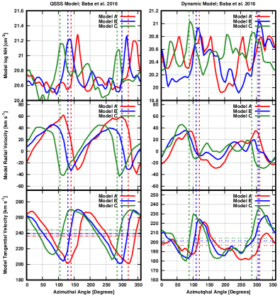
Figure 9: Azimuthal distribution of the column density (top panel), radial velocity (middle panel), and tangential velocities (bottom panel) resulting from the QSSS and dynamical models presented by Baba et al. (2016, see also their Figure 4 for further details). We also show in the location of the spiral potential and the average tangential velocities as vertical and horizontal lines, respectively.

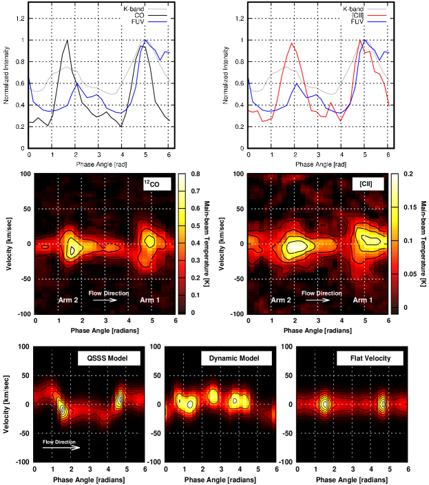
Figure 10: (Upper panels) Integrated intensity distribution of ¹²CO (left) and [C ii] (right) as a function of azimuthal angle between 2.6 kpc and 3.7 kpc from M51’s center. We also include the azimuthal distribution of FUV and NIR K–band emission in both panels. (Middle panels) Position–velocity map of the ¹²CO (left) and [C ii] (right) emission across the spiral arms between 2.6 kpc and 3.7 kpc from M51’s center. (Bottom panels) Simulated position–velocity maps predicted from the QSSS (left) and dynamical (middle) models by Baba et al. (2016). We also include a purely circular rotation model (right). The flow direction goes from left to right, as indicated by the white arrow.

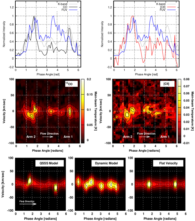
Figure 11: (Upper panels) Integrated intensity distribution of ¹²CO (left) and [C ii] (right) as a function of azimuthal angle between 6.9 kpc and 7.9 kpc from M51’s center. We also include the azimuthal distribution of FUV and NIR K–band emission in both panels. (Middle panels) Position–velocity map of the ¹²CO (left) and [C ii] (right) emission across the spiral arms between 6.9 kpc and 7.9 kpc from M51’s center. (Bottom panels) Simulated position–velocity maps predicted from the QSSS (left) and dynamical (middle) models by Baba et al. (2016). We also include a purely circular rotation model (right). The flow direction goes from left to right, as indicated by the white arrow.

We investigate whether the observed position velocity distribution of CO and [C ii] is consistent with the existence of galactic shocks by comparing our observed position–velocity distributions across spiral arms with those predicted by theoretical models of the nature of spiral arms in galaxies. Baba et al. (2016) studied velocity patterns in hydrodynamical simulations of galaxies with QSSS and dynamical spirals arms. These simulations include self–gravity, radiative cooling, heating due to the interstellar FUV radiation field, and include a sub–grid model for star formation and stellar feedback. They presented azimuthal distributions of column density, tangential and radial velocity profiles for three different distances to the center of the model galaxies, that are well within the co-rotation radius ($R<0.5R_{\rm cr}$), and are separated by 1 kpc. We denote these three models, in order of increasing distance to the model galaxy’s center, as Model A, B, and C. In Figure 9, we show the azimuthal distribution of the column density, radial velocity, and tangential velocities resulting from the QSSS and dynamical models presented by Baba et al. (2016, see their Figure 4 for further details). We also show in Figure 9, the location of the spiral potential and the average tangential velocities as vertical and horizontal lines, respectively. Spiral arms are manifested as peaks in the column density distribution, with the QSSS model showing gas peaks downstream from the spiral potential peak with offsets that increase with the distance to the galactic center, as expected for this theory inside the co–rotation radius, while in the dynamic model no systematic offset is seen. The shape of the radial and tangential profiles in both models are unaffected by different galactocentric distances. In the QSSS model we see a periodic azimuthal distribution of both radial and tangential velocities, with spiral arms being associated with the radial velocity minimum and the average tangential velocity. In contrast, the dynamical model the spiral arms are associated with zero radial velocities and tangential velocities that are higher than their average.

We compare our observations with the predictions from Baba et al. (2016) by creating model galaxies with projected velocity structures that follows the radial and tangential velocity profiles of dynamical and steady models as shown in Figure 9. We also generate a purely circular model, i.e. with no velocity structure other than rotation, with the aim of determining whether any systematics in our method affects the shape of the position velocity distribution in spiral arms. The model galaxies are assumed to be at the same distance to M51 and have the same inclination, $i$, position angle, $\theta_{\it MA}$, systemic velocity of the galaxy, $V_{\rm sys}$ (Table 1). We calculate the projected velocities using

$$V=V_{sys}+[V_{\it R}\sin(\theta-\theta_{\it MA})+V_{\it T}\cos(\theta-\theta_{\it MA})]\sin(i),$$ (7)

where $V_{\it R}$ and $V_{\it T}$ are the predicted radial and tangential velocities (from Figure 9), respectively. For each pixel we assumed Gaussian line profiles with a FWHM line width of 30 km s^-1 (typical of our [C ii] data) and peak intensities given by $T_{\rm peak}=N_{\rm H}/{\rm FWHM}$, where $N_{\rm H}$ is the hydrogen column density predicted by the models shown in Figure 9. We generate two sets of simulated galaxies with spiral arms with pitch angles that correspond to those in M51’s inner and outer galaxy (Table 2). To correct the projected model velocities to a reference frame that rotates with the spiral potential, we also produce a map of projected velocities in which $V_{\it R}=0$ km s^-1 and $V_{\it T}$ is equal to the rotation velocity of the galaxy. The tangential velocity shown in Figure 9 can be decomposed into the rotation velocity plus peculiar velocities due to the spiral arm perturbation. As we did with the M51 data, we set the velocity axis of the simulated data cubes to be $V=0$ km s^-1 at the projected velocity of the purely rotating map. We show the position–velocity resulting from QSSS and Dynamic Model A, together with observations, in Figure 10 and 11 for rings in the inner and outer galaxy, respectively. In Figure 12 and 13, we also illustrate the predicted position velocity maps for Model A, B, and C, for the inner and outer galaxy rings shown in Figure 10 and 11, respectively. In Appendix A we study the sensitivity of the QSSS predicted velocity patterns on the amplitude of radial and tangential motions and on the spatial location of spiral arms in the galaxy.

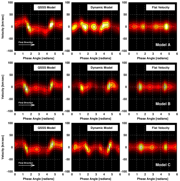
Figure 12: Projected position–velocity maps of model galaxies with quasi–static (QSSS model) and dynamic spiral (Dynamic Model) arms presented by Baba et al. (2016) for Model A, B, and C (Section 4.2.1). We also include a galaxy with no velocity structure other than pure rotation (Flat Velocity). The predicted velocities are projected to correspond to that observed at a ring between 2.6 kpc and 3.7 kpc from the center of M51 (see Figure 10).

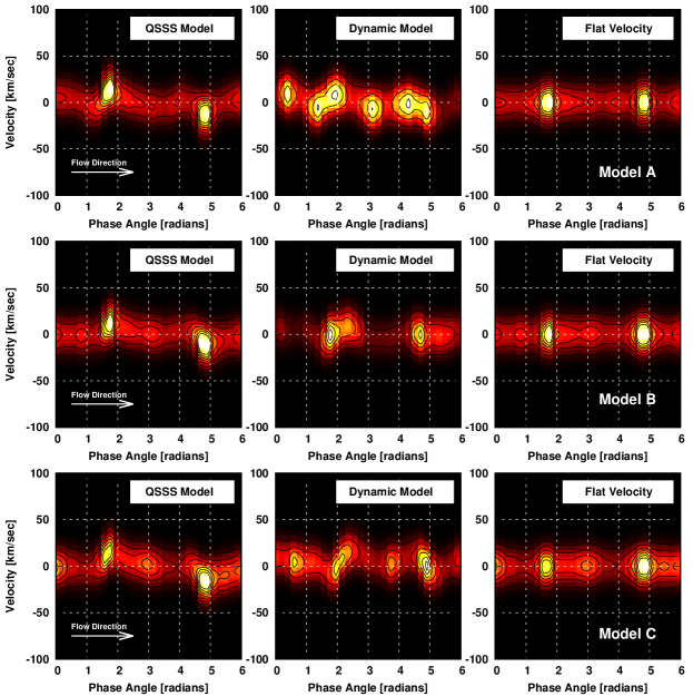
Figure 13: Projected position–velocity maps of model galaxies with quasi–static (QSSS model) and dynamic spiral (Dynamic Model) arms presented by Baba et al. (2016) for Model A, B, and C (Section 4.2.1). We also include a galaxy with no velocity structure other than pure rotation (Flat Velocity). The predicted velocities are projected to correspond to that observed at a ring between 6.9 kpc and 7.9 kpc from the center of M51 (see Figure 11).

In Figure 10, we show the position–velocity distribution of [C ii] and CO across spiral arms between 2.6 kpc and 3.7 kpc from M51’s center. We also include the distribution of [C ii] and ¹²CO integrated intensities as a function of phase angle and predictions for this region simulated from Model A of Baba et al. (2016) and for a model galaxy with no peculiar velocity other than its rotation. We also include the NIR K–band distribution, denoting the location of the bottom of the gravitational potential, and FUV emission tracing evolved star formation regions. The observed position velocity maps show an antisymmetric pattern with a velocity gradient observed in both tracers. Following the flow direction from left to right, the gas velocity increases and then decreases in the first (left) spiral arm and later the velocity is reduced and then increased at the location of the second spiral arm (right). The CO intensity peaks at the location of the second velocity gradient in both arms. The [C ii] intensity peaks downstream from the CO peak in both spiral arms. Note that in the integrated intensity distribution for this ring, we see no noticeable offset between ¹²CO and [C ii] for Arm 1, while there is a clear offset in the position velocity maps. This discrepancy is due to the variation of the line–widths as a function of phase angle, which results in a broader integrated intensity distribution across the arm, which makes it difficult for offsets to be identified in the position-position space. As we can see, the QSSS model shows also an antisymmetric pattern in which the velocity increases and then decreases in the first spiral arm and then decreases and subsequently increases at the location of the second spiral arm. For the dynamical model we see variations in the velocity field but we do not see the antisymmetric pattern that is observed and predicted by the QSSS model. Further evidence supporting the QSSS model is the fact that we see a displacement in position velocity space between CO and [C ii], with the latter, which traces star formation, being downstream from the dense molecular gas traced by CO. This result is a prediction of the QSSS model that is not seen in the dynamical model. In the latter model, the gas is expected to flow from both sides of the arm, and thus no relative displacement in these tracers are expected. We therefore conclude that the spiral structure observed in this area in M51 is consistent with the QSSS spiral model. Note that what we observe here is the shock and gas phase changes across the spiral arms, and therefore, the events that occur over arm–crossing timescales. Therefore, we cannot exclude a possibility that the ”QSSS” spiral arms might move and evolve over a much longer timescale.

The projected position–velocity maps derived from Model A of Baba et al. (2016), shown in the bottom panels in Figure 11, also show velocity gradient that is opposite to that seen in the inner galaxy, due to the different direction of the flow with respect to the spiral arms. For Arm 2, we find a resemblance between the observations and predictions from the QSSS theory. We observe a velocity gradient for the predictions for the dynamic spiral at this radii, but the magnitude of the velocity variation is smaller than that observed. Additionally, this velocity variation is not present for predictions in the other models from Baba et al. (2016), as shown in Figure 13. The offsets between ¹²CO and [C ii] again suggest that Arm 2 is consistent with the predictions from the QSSS theory. However, the lack of velocity structure in Arm 1 would also allow for the dynamic spiral mechanism to govern the structure of this spiral arm in the outer regions of M51. This spiral arm is pointing away from the companion in the outer galaxy, and therefore is feeling less of the direct tidal pull, perhaps making it more flocculent in nature.

Note that our comparison with the Baba et al. (2016) calculations is qualitative, as their model parameters do not necessarily match those of the M51 galaxy. The QSSS is triggered when the rotation speed of a spiral potential is slower/faster than that of gas, and the dynamical spiral arm is governed primarily by the swing amplification due to epicyclic motions. These two physical mechanisms can operate in any spiral galaxy, and hence the two models are expected to make qualitative differences independent of the total stellar and gas masses of a galaxy and its rotation curve. In particular, their method was developed for isolated galaxies, while M51 is affected by the interaction with the M51b galaxy (Pettitt et al., 2017; Tress et al., 2019). The companion galaxy may be causing a significant $m=2$ mode perturbation, which may make M51 a special case, and there are suggestions that in tidally interacting systems shocks similar to those predicted by the QSSS theory could be present (Oh et al., 2008; Dobbs et al., 2010; Oh et al., 2015). To any extent, this is a case study, and we need a larger sample of galaxies to draw a general conclusion on the mechanism for driving spiral arms.

4.2.2 Comparison with previous studies of the nature of spiral arms in M51

Another test for distinguishing between different theories of the nature of spiral arms in galaxies is the distribution of star clusters age across spiral arms. Dobbs & Pringle (2010) presented numerical simulations for galaxies with QSSS, dynamic spirals, a barred galaxy, and an interacting galaxies like M51. They find that in the case of the QSSS and barred–galaxy, stellar clusters are predicted to show offsets from the spiral arms that increase with age, as stars and gas rotate faster than the spiral pattern, and stars formed after the compression of gas in the spiral arms eventually overtake the spiral pattern as they age. In the case of the dynamic model, stars form as a result of local gas instabilities, and thus no age gradient is expected. They also predicted that for an interacting system, no clear stellar gradient is expected, due to the complex dynamics of the interaction. These theoretical predictions have been tested with optical observations in M51. Chandar et al. (2017) used an optically derived catalog of star cluster ages to study their distribution across M51’s spiral arms. They observe that young stellar clusters ($<$10 Myr) are preferentially observed near the arms, but intermediate age (10–50 Myr) and old (50–100 Myr) have a more spread distribution. While they find an offset between CO emission and young ($<$10 Myr) stellar clusters, which they interpreted as to be in agreement with QSSS spirals, they do not find a significant offsets from the spiral arms for older stellar clusters. Shabani et al. (2018) used a similar data set in M51 and also found no significant offsets in the location of stellar clusters across the arms of M51, suggesting that the dynamic model would also explain the nature of spiral arms in M51. Note, however, that for a rotation velocity of $\sim$200 km s^-1 (Meidt et al., 2013; Oikawa & Sofue, 2014), in the inner M51 ($R=3.2$ kpc; see Figure 10) it would take a newly formed cluster only $\sim$40 Myr to move from one arm to another, and therefore the young clusters observed near spiral arms are likely mixed with older clusters formed in the other spiral arm, or in the inter–arm regions, where CO and [C ii] emission is also detected. The rapid spatial mixing in the inner M51 makes the observation of a cluster age gradient difficult and therefore creates an ambiguity on whether stellar cluster age observations can be explained with the QSSS or dynamic model. The observed CO velocity pattern and offset between CO and [C ii] provides an alternative evidence that QSSS is producing the spiral arms in M51.

Based on the rotation velocity mentioned above, and the observed offsets in phase angle, it would take the gas about $\sim$5 Myr to move between the CO and [C ii] peaks in the position–velocity maps. The [C ii] peak in the position–velocity maps is likely associated with the embedded star formation phase (lasting for about 1.5 Myr; e.g. Kruijssen et al., 2019), as it is located downstream from CO but upstream from FUV emission peaks, tracing the dense gas phase prior to star formation and the cloud dispersal by stellar feedback phase, respectively. Therefore, the observed offset between CO and [C ii] peaks in position–velocity space suggest a star formation timescale of about 5 Myr.

5 Summary

In this paper, we studied the influence of spiral density waves on the evolution of the interstellar medium and star formation in the M51 galaxy. We used new spectrally resolved upGREAT/SOFIA [C ii] data combined with NIR K–band, FUV, H i, and CO data to study the spatial and spatial–velocity distribution of different ISM phases in the spiral arms of M51. Our results can be summarized as follows:

• We identify azimuthal offsets between NIR K–band, ¹²CO, [C ii], and FUV, tracing stellar mass, dense and cold molecular gas, obscured star formation, and unobscured star formation, respectively, in the spiral arms of M51. However, we could not find systematic variations of these offsets with galactocentric distance at the angular resolution of our observations.

• The offsets between ¹²CO and [C ii] in M51 are more apparent in Arm 2, connecting to the companion galaxy M51b, compared with Arm 1, pointing away from the companion. We find that identifying offsets between ¹²CO and [C ii] integrated intensities is complicated by the varying line widths of these tracers at the location of spiral arms, and that they are better separated when comparing peak main beam temperatures in the position velocity space.

• The position velocity maps of H i, ¹²CO, and [C ii] across spiral arms in M51 show strong velocity gradients at the location of stellar arms (traced by K–band data) with a clear offset in position velocity space between upstream molecular gas (traced by ¹²CO) and downstream star formation (traced by [C ii]).

• We compared the observed position velocity maps across spiral arms with simulated observations from numerical simulations of galaxies with both dynamical and quasi–stationary steady spiral arms that predict tangential and radial velocities at the location of spiral arms. We find that our observations are consistent with the presence of spiral shock in spiral arms in the inner M51 and in the arm connecting to the companion galaxy, M51b, in the outer M51 (Arm 2).

Our analysis shows that spectrally resolved observations are important tools for studying kinematics of spiral arms and the evolution of the interstellar medium in galaxies. They are also useful for distinguishing between competing theories of the nature of spiral structure in galaxies. We speculate that the spiral shocks observed in M51 might originate as a result of the interaction between M51 and M51b. A better test for theories of spiral structure in isolated galaxies would be to apply the techniques described in this paper to velocity resolved [C ii] and CO observations of systems that have not been influenced by tidal interaction. Both [C ii] and CO are needed to distinguish between steady and dynamic spirals, as the velocity gradients predicted for steady spirals can be mimicked by dynamic spirals. However, the observed offsets between [C ii] and CO, which are often only seen in position velocity space and are predicted only by the QSSS theory, were able to break the ambiguity between these models.

Appendix A Dependence of position–velocity patterns on tangential and radial velocity amplitudes, and location in the galaxy.

The similarity between the observed and QSSS model–predicted velocity distribution motivate us to use model–predicted radial and tangential velocities to investigate under what conditions the observed velocity profiles are produced. In the left panel of Figure 14, we show the position peak velocity maps for Baba et al. (2016) Model A, where we multiplied the radial velocity by factors of 0.5, 1, 1.5, and 2, while keeping the tangential velocity distribution as predicted by the model. The projected velocity is determined using Equation 6 and subtracting the projected velocity in the case when only the galaxy rotation is present. Increasing the amplitude of the radial velocity results in larger velocity gradients in the position velocity maps. As discussed in Section 4.2.1 above, in the QSSS model the spiral arms are associated with V_r minima and V_t close to its average, and thus the contribution from the radial velocity to the projected velocity is maximized at the location of spiral arms. In the middle panel of Figure 14, we show the position–velocity maps for Model A in the case where the tangential velocity is multiplied by factors of 0.5, 1, 1.5, and 2, while keeping the radial velocity distribution as predicted by the model. Note that in this case we vary the amplitude of the tangential velocity with respect to its average value, as it also includes the rotation of the galaxy. No significant change in the position velocity maps is observed in this case.

Another important condition for QSSS velocity patterns to be observable is the azimuthal angle of spiral arms for a given radius. In the inner M51, the azimuthal angles of the spiral arms where we see a velocity gradient (between 2.6 kpc and 3.7 kpc; Figure 10) are $\theta\simeq 124\arcdeg$ and $34\arcdeg$ for Arm 1 and Arm 2, respectively. These azimuthal angles correspond to about $\Delta\theta=+45$° and $-$45° offsets from the minor axis for Arm 1 and Arm 2, respectively. In the outer galaxy location where we see a velocity gradient (between 6.9 kpc and 7.9 kpc; Figure 11) the azimuthal angle of Arm 2 is 158°, which is about $\Delta\theta\simeq-11.7$° from the minor axis. In the right panel of Figure 14, we show the predicted position velocity profiles for the QSSS Model A galaxy with the same azimuthal angle as that observed in the inner M51. We also show the position–velocity distribution for spiral arms located being rotated by $\Delta\theta=-$45°(i.e located at the minor axis) and $+45$°(i.e. located 90° from the minor axis). Note that we moved the origin of the phase angle distribution by the same azimuthal angles shown in the figure to keep the location of spiral arms in phase angle constant. We see that for an azimuthal angle of the arms that are at the location of the minor axis (offset by $-$45°) the projected velocity gradient shows the largest amplitude, but it dissapears when we rotate the spiral ams by an offset of $+$45° from the location where we see the arms in the inner M51. From Equation (7) we see that the contribution from the radial velocity is maximized, and the contribution of the tangential velocity is minimized, at locations close to the minor axes ($\sin(\theta-\theta_{\rm MA})\simeq 1$). As shown above, the velocity gradients seen in the projected velocity in the QSSS model mostly depend on the radial velocity and thus the observed the pattern is expected in rings where the arms are at an azimuthal angle that maximizes the contribution from the radial velocity to the projected velocity.

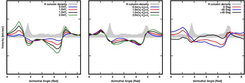
Figure 14: (Left panel) Projected velocity as a function of phase angle derived from the QSSS Model A in Baba et al. (2016), with the radial velocity contribution being factored by factors of 0.5, 1, 1.5, and 2, and the tangential velocity contribution kept as predicted by the model. (Middle panel) Projected velocity as a function of phase angle taken from QSSS Model A, with the tangential velocity contribution multiplied by factors of 0.5, 1, 1.5, and 2, and the radial velocity contribution kept as predicted by the model. (Right panel) Projected velocity as a function of phase angle, again taken from QSSS Model A, but with the angular location being rotated by $-$45 and $+$45 degrees from the location of the spiral arms for a radius between 2.6  and 3.7 kpc in our simulated M51 galaxy. In all panels we also show the hydrogen column density distribution as a function of phase angle from QSSS Model A to denote the location of spiral arms peaks.

References

- Aalto et al. (1999) Aalto, S., Hüttemeister, S., Scoville, N. Z., & Thaddeus, P. 1999, ApJ, 522, 165, doi: 10.1086/307610
- Allen (2002) Allen, R. J. 2002, in Astronomical Society of the Pacific Conference Series, Vol. 276, Seeing Through the Dust: The Detection of HI and the Exploration of the ISM in Galaxies, ed. A. R. Taylor, T. L. Landecker, & A. G. Willis, 288
- Baba et al. (2016) Baba, J., Morokuma-Matsui, K., Miyamoto, Y., Egusa, F., & Kuno, N. 2016, MNRAS, 460, 2472, doi: 10.1093/mnras/stw987
- Baba et al. (2013) Baba, J., Saitoh, T. R., & Wada, K. 2013, ApJ, 763, 46, doi: 10.1088/0004-637X/763/1/46
- Bertin & Lin (1996) Bertin, G., & Lin, C. C. 1996, Spiral structure in galaxies a density wave theory, ISBN0262023962
- Bigiel et al. (2016) Bigiel, F., Leroy, A. K., Jiménez-Donaire, M. J., et al. 2016, ApJ, 822, L26, doi: 10.3847/2041-8205/822/2/L26
- Binney & Merrifield (1998) Binney, J., & Merrifield, M. 1998, Galactic Astronomy
- Bolatto et al. (2013) Bolatto, A. D., Wolfire, M., & Leroy, A. K. 2013, ARA&A, 51, 207, doi: 10.1146/annurev-astro-082812-140944
- Chandar et al. (2017) Chandar, R., Chien, L. H., Meidt, S., et al. 2017, ApJ, 845, 78, doi: 10.3847/1538-4357/aa7b38
- Daigle et al. (2006) Daigle, O., Carignan, C., Amram, P., et al. 2006, MNRAS, 367, 469, doi: 10.1111/j.1365-2966.2006.10002.x
- Dobbs & Baba (2014) Dobbs, C., & Baba, J. 2014, PASA, 31, e035, doi: 10.1017/pasa.2014.31
- Dobbs & Pringle (2010) Dobbs, C. L., & Pringle, J. E. 2010, MNRAS, 409, 396, doi: 10.1111/j.1365-2966.2010.17323.x
- Dobbs et al. (2010) Dobbs, C. L., Theis, C., Pringle, J. E., & Bate, M. R. 2010, MNRAS, 403, 625, doi: 10.1111/j.1365-2966.2009.16161.x
- D’Onghia et al. (2013) D’Onghia, E., Vogelsberger, M., & Hernquist, L. 2013, ApJ, 766, 34, doi: 10.1088/0004-637X/766/1/34
- Duarte-Cabral et al. (2015) Duarte-Cabral, A., Acreman, D. M., Dobbs, C. L., et al. 2015, MNRAS, 447, 2144, doi: 10.1093/mnras/stu2586
- Egusa et al. (2017) Egusa, F., Mentuch Cooper, E., Koda, J., & Baba, J. 2017, MNRAS, 465, 460, doi: 10.1093/mnras/stw2710
- Fletcher et al. (2011) Fletcher, A., Beck, R., Shukurov, A., Berkhuijsen, E. M., & Horellou, C. 2011, MNRAS, 412, 2396, doi: 10.1111/j.1365-2966.2010.18065.x
- Foyle et al. (2011) Foyle, K., Rix, H. W., Dobbs, C. L., Leroy, A. K., & Walter, F. 2011, ApJ, 735, 101, doi: 10.1088/0004-637X/735/2/101
- Gil de Paz et al. (2007) Gil de Paz, A., Boissier, S., Madore, B. F., et al. 2007, ApJS, 173, 185, doi: 10.1086/516636
- Gittins & Clarke (2004) Gittins, D. M., & Clarke, C. J. 2004, MNRAS, 349, 909, doi: 10.1111/j.1365-2966.2004.07560.x
- Goldreich & Lynden-Bell (1965) Goldreich, P., & Lynden-Bell, D. 1965, MNRAS, 130, 125, doi: 10.1093/mnras/130.2.125
- Goldsmith et al. (2012) Goldsmith, P. F., Langer, W. D., Pineda, J. L., & Velusamy, T. 2012, ApJS, 203, 13, doi: 10.1088/0067-0049/203/1/13
- Grenier et al. (2005) Grenier, I. A., Casandjian, J.-M., & Terrier, R. 2005, Science, 307, 1292, doi: 10.1126/science.1106924
- Jarrett et al. (2003) Jarrett, T. H., Chester, T., Cutri, R., Schneider, S. E., & Huchra, J. P. 2003, AJ, 125, 525, doi: 10.1086/345794
- Kennicutt et al. (2003) Kennicutt, Jr., R. C., Armus, L., Bendo, G., et al. 2003, PASP, 115, 928, doi: 10.1086/376941
- Klessen & Glover (2016) Klessen, R. S., & Glover, S. C. O. 2016, Saas-Fee Advanced Course, 43, 85, doi: 10.1007/978-3-662-47890-5_2
- Koda et al. (2009) Koda, J., Scoville, N., Sawada, T., et al. 2009, ApJ, 700, L132, doi: 10.1088/0004-637X/700/2/L132
- Koda et al. (2012) Koda, J., Scoville, N., Hasegawa, T., et al. 2012, ApJ, 761, 41, doi: 10.1088/0004-637X/761/1/41
- Kruijssen et al. (2019) Kruijssen, J. M. D., Schruba, A., Chevance, M., et al. 2019, Nature, 569, 519, doi: 10.1038/s41586-019-1194-3
- Langer et al. (2010) Langer, W. D., Velusamy, T., Pineda, J. L., et al. 2010, A&A, 521, L17, doi: 10.1051/0004-6361/201015088
- Louie et al. (2013) Louie, M., Koda, J., & Egusa, F. 2013, ApJ, 763, 94, doi: 10.1088/0004-637X/763/2/94
- McQuinn et al. (2016) McQuinn, K. B. W., Skillman, E. D., Dolphin, A. E., Berg, D., & Kennicutt, R. 2016, ApJ, 826, 21, doi: 10.3847/0004-637X/826/1/21
- Meidt et al. (2013) Meidt, S. E., Schinnerer, E., García-Burillo, S., et al. 2013, ApJ, 779, 45, doi: 10.1088/0004-637X/779/1/45
- Mentuch Cooper et al. (2012) Mentuch Cooper, E., Wilson, C. D., Foyle, K., et al. 2012, ApJ, 755, 165, doi: 10.1088/0004-637X/755/2/165
- Miyamoto et al. (2014) Miyamoto, Y., Nakai, N., & Kuno, N. 2014, PASJ, 66, 36, doi: 10.1093/pasj/psu017
- Mutchler et al. (2005) Mutchler, M., Beckwith, S. V. W., Bond, H., et al. 2005, in Bulletin of the American Astronomical Society, Vol. 37, American Astronomical Society Meeting Abstracts #206, 452
- Nikola et al. (2001) Nikola, T., Geis, N., Herrmann, F., et al. 2001, ApJ, 561, 203, doi: 10.1086/323235
- Oh et al. (2015) Oh, S. H., Kim, W.-T., & Lee, H. M. 2015, ApJ, 807, 73, doi: 10.1088/0004-637X/807/1/73
- Oh et al. (2008) Oh, S. H., Kim, W.-T., Lee, H. M., & Kim, J. 2008, ApJ, 683, 94, doi: 10.1086/588184
- Oikawa & Sofue (2014) Oikawa, S., & Sofue, Y. 2014, PASJ, 66, 77, doi: 10.1093/pasj/psu059
- Parkin et al. (2013) Parkin, T. J., Wilson, C. D., Schirm, M. R. P., et al. 2013, ApJ, 776, 65, doi: 10.1088/0004-637X/776/2/65
- Pettitt et al. (2017) Pettitt, A. R., Tasker, E. J., Wadsley, J. W., Keller, B. W., & Benincasa, S. M. 2017, MNRAS, 468, 4189, doi: 10.1093/mnras/stx736
- Pety et al. (2013) Pety, J., Schinnerer, E., Leroy, A. K., et al. 2013, ApJ, 779, 43, doi: 10.1088/0004-637X/779/1/43
- Pineda et al. (2013) Pineda, J. L., Langer, W. D., Velusamy, T., & Goldsmith, P. F. 2013, A&A, 554, A103, doi: 10.1051/0004-6361/201321188
- Pineda et al. (2018) Pineda, J. L., Fischer, C., Kapala, M., et al. 2018, ApJ, 869, L30, doi: 10.3847/2041-8213/aaf1ad
- Querejeta et al. (2019) Querejeta, M., Schinnerer, E., Schruba, A., et al. 2019, A&A, 625, A19, doi: 10.1051/0004-6361/201834915
- Risacher et al. (2016) Risacher, C., Güsten, R., Stutzki, J., et al. 2016, A&A, 595, A34, doi: 10.1051/0004-6361/201629045
- Roberts & Stewart (1987) Roberts, Jr., W. W., & Stewart, G. R. 1987, ApJ, 314, 10, doi: 10.1086/165035
- Schinnerer et al. (2013) Schinnerer, E., Meidt, S. E., Pety, J., et al. 2013, ApJ, 779, 42, doi: 10.1088/0004-637X/779/1/42
- Shabani et al. (2018) Shabani, F., Grebel, E. K., Pasquali, A., et al. 2018, MNRAS, 478, 3590, doi: 10.1093/mnras/sty1277
- Shetty et al. (2007) Shetty, R., Vogel, S. N., Ostriker, E. C., & Teuben, P. J. 2007, ApJ, 665, 1138, doi: 10.1086/520037
- Smith et al. (2014) Smith, R. J., Glover, S. C. O., Clark, P. C., Klessen, R. S., & Springel, V. 2014, MNRAS, 441, 1628, doi: 10.1093/mnras/stu616
- Tamburro et al. (2008) Tamburro, D., Rix, H.-W., Walter, F., et al. 2008, AJ, 136, 2872, doi: 10.1088/0004-6256/136/6/2872
- Toomre & Toomre (1972) Toomre, A., & Toomre, J. 1972, ApJ, 178, 623, doi: 10.1086/151823
- Tress et al. (2019) Tress, R. G., Smith, R. J., Sormani, M. C., et al. 2019, arXiv e-prints, arXiv:1909.10520. https://arxiv.org/abs/1909.10520
- Walter et al. (2008) Walter, F., Brinks, E., de Blok, W. J. G., et al. 2008, AJ, 136, 2563, doi: 10.1088/0004-6256/136/6/2563
- Wannier et al. (1991) Wannier, P. G., Andersson, B. G., Morris, M., & Lichten, S. M. 1991, ApJS, 75, 987, doi: 10.1086/191557
- Wolfire et al. (2010) Wolfire, M. G., Hollenbach, D., & McKee, C. F. 2010, ApJ, 716, 1191, doi: 10.1088/0004-637X/716/2/1191
- Young et al. (2012) Young, E. T., Becklin, E. E., Marcum, P. M., et al. 2012, ApJ, 749, L17, doi: 10.1088/2041-8205/749/2/L17