Calculation of transverse momentum dependent distributions beyond the leading power

Abstract

We compute the contribution of twist-2 and twist-3 parton distribution functions to the small-$b$ expansion for transverse momentum dependent (TMD) distributions at all powers of $b$. The computation is done by the twist-decomposition method based on the spinor formalism for all eight quark TMD distributions. The newly computed terms are accompanied by the prefactor $(M^{2}b^{2})^{n}$ and represent the target-mass corrections to the resummed cross-section. For the first time, a non-trivial expression for the pretzelosity distribution is derived.

1 Introduction

Transverse momentum dependent (TMD) distributions extend the parton model, including the transverse motion of hadron’s constituents. Any TMD distribution is a function of two dynamical variables $x$ and $b$. The variable $x$ is the fraction of hadron’s momentum carried by the parton. The variable $b$ is the transverse distance that is Fourier conjugated to the transverse momentum of parton $k_{T}$. In the limit $b\to 0$, which corresponds to integrated or unobserved transverse momentum, a TMD distribution turns to the corresponding collinear parton distribution functions (PDFs) or fragmentation function (FFs). Technically, this relation, which is also known as the matching between TMD parton distribution functions (TMDPDFs) and PDFs (or TMD fragmentation functions (TMDFFs) and FFs), is received by the operator product expansion, and its leading power term is very well studied. In the present work, we extend this formalism beyond the leading power term and compute matching of TMDPDFs to PDFs of twist-2 and twist-3 at all powers of $b^{2}$-expansion.

The matching of TMDPDFs to PDFs is an important part of the TMD factorization approach. The review of various aspects of TMD factorization can be found in Collins:2011zzd ; Angeles-Martinez:2015sea ; Scimemi:2019mlf . On the theory side, the matching establishes the connection with the resummation formalism and allows interpolation between TMD factorized cross-section and fixed order computations, see f.i. Becher:2010tm ; Gehrmann:2014yya ; Collins:2016hqq . On the phenomenological side, the matching essentially reduces the parametric freedom for TMD ansatzes. The modern phenomenology of TMD distributions is grounded on the matching relations and demonstrates perfect agreement with the large amount of experimental data Scimemi:2019cmh ; Bacchetta:2019sam .

So far, all studies of matching relations were restricted to the leading power term only. The leading power term is the most simple and numerically dominant contribution. Nonetheless, several aspects make the study of power corrections interesting. First of all, such a study carries a significant amount of methodological novelty. Indeed, the power corrections are generally considered as a complicated field, and their computation is an interesting theoretical task. In this work, we have computed the whole series of power correction with PDFs of twist-2 and twist-3, which is almost unprecedented. Methodologically, the closest example of similar computation is the computation of kinematic power corrections to Deeply Virtual Compton Scattering (DVCS) made by Braun and Manashov in ref.Braun:2011dg . The second point of interest is the derivation of the matching relations for polarized TMD distributions. For many TMD distributions already, the leading power matching involves twist-3 functions and requires a non-trivial computation. The computations for different TMDPDFs have been made by different methods in refs.Boer:2003cm ; Ji:2006ub ; Kang:2011mr ; Kanazawa:2015ajw . In ref.Scimemi:2018mmi , all polarized TMDPDFs were systematically computed in a single scheme, and the agreement with previous computations had been shown. However, all these computations were unable to find the non-trivial matching of the pretzelosity distribution, which is derived for the first time in this work. The third point of interest is the comparison of the derived power corrections to the extracted ones. There are many examples, where the part of the power correction proportional to twist-2 PDFs (Wandzura-Wilczek approximation) is numerically dominant Accardi:2009nv . However, there are also known cases of opposite behavior. In this work, we demonstrate that TMD distributions belong to the latter case, and for them, the contribution of higher twist PDFs is essential. The forth point of interest is the target-mass dependence of TMD distributions. At higher powers of small-$b$ series, the target mass is the only scale that compensates the dimension of $b^{n}$ for twist-2 and twist-3 distributions. Thus, the here derived corrections are target-mass corrections $\sim(M^{2}b^{2})$. Their knowledge is essential since much of the experimental data is measured on nuclei.

Formally, the matching is obtained by operator product expansion of the transverse momentum dependent operator (defined explicitly in (40)) at small values of $b$. The later has the schematic form

$$O^{\text{TMD}}(z,b) = \mathbb{O}_{2}(z)+b_{\mu}\mathbb{O}_{3}^{\mu}(z)+\frac{b_{\mu_{1}}b_{\mu_{2}}}{2}\mathbb{O}_{4}^{\mu_{1}\mu_{2}}(z)+...=\sum_{n=0}^{\infty}\frac{b_{\mu_{1}}...b_{\mu_{n}}}{n!}\mathbb{O}_{n+2}^{\mu_{1}...\mu_{n}}(z),$$ (1)

where $z$ is the distance between fields of the operator along the light-cone. The operators $\mathbb{O}_{n}(z)$ are light-cone operators with the collinear twist $n$. For example, the leading power operator is $\mathbb{O}_{2}(z)\sim\bar{q}(zn)[zn,0]q(0)$, where $n$ is the light-cone vector, $[a,b]$ is the straight gauge link, and $q$ is the quark field. Each operator $\mathbb{O}_{n}$ is the integral convolution of a coefficient function and an actual quantum-field operator. The coefficient functions for $\mathbb{O}_{2}$ are all known at next-to-leading order (NLO) in $\alpha_{s}$-expansion Gutierrez-Reyes:2017glx ; Buffing:2017mqm , and NNLO Gehrmann:2014yya ; Echevarria:2016scs ; Gutierrez-Reyes:2018iod ; Gutierrez-Reyes:2019rug . The leading power coefficient function for unpolarized distribution has been recently computed at N³LO Luo:2019szz ; Ebert:2020yqt . Beyond the leading power the information is sparse. The tree order matching for $\mathbb{O}_{3}$ has been derived in Scimemi:2018mmi , see also Boer:2003cm ; Ji:2006ub ; Kang:2011mr ; Kanazawa:2015ajw for particular cases. The only NLO computation for $\mathbb{O}_{3}$ is made for the Sivers function Scimemi:2019gge . In this work, we derive only the tree order matching, ignoring the $\alpha_{s}$-suppressed terms in the coefficient functions. For that reason, we do not specify the renormalization scales and omit corresponding arguments.

The operators with the collinear twist $n$ can be presented as a sum of operators with different geometrical twists,

$$\mathbb{O}_{n}(z)=\sum_{t=2}^{n}C_{t}(z;\{y\})\otimes O_{t}(\{y\}),$$ (2)

where we omit indices $\mu_{1}...\mu_{n}$ for brevity. For shortness, we call this procedure as twist-decomposition. Generally, operators $O_{t}$ depend on many spatial points, which are parameterized by a set of variables $\{y\}$. They are mapped to the single variable $z$ by the integral convolution $\otimes$. The geometric twist has a strict definition as the “dimension minus spin” of the operator. Operators with different geometrical twists have different transformation properties and thus represent independent physical observables. The matrix elements of operators with a given geometrical twist define a self-contained set of PDFs. Such a set of PDFs does not mix with other sets, and their evolution is autonomous. For the introduction to the twist decomposition see e.g.Jaffe:1996zw ; Braun:2003rp , the review of modern development can be found in Braun:2011dg . Therefore, the central task is to derive the twist-decomposition for each operator on the right-hand-side (RHS) of (1). In turn, the small-$b$ expansion of TMDPDFs in terms of collinear PDFs is received by evaluating the matrix element over the derived operator relation.

In the case of FF, the twist-decomposition operation is not well defined. The main reason is the absence of local expansion for fragmentation operators. In ref.Balitsky:1990ck it has been shown that OPE for FF is defined up to terms that satisfy the Laplace equation (for the twist-2 part). Therefore, alternative methods such as differential equations Balitsky:1990ck , Feynman diagram correspondences Kanazawa:2013uia ; Echevarria:2015usa ; Echevarria:2016scs ; Gamberg:2018fwy and Lorentz invariant relations Kanazawa:2015ajw , should be used. For that reason, we do not consider the matching of TMDFFs to FFs in the present work. For an interested reader, we present some discussion on power corrections for TMDFF in appendix B.

In this work, we compute only quark TMD distributions, since they are of the prime practical interest. In total, there are eight TMDPDFs at the leading term of the factorization theorem Mulders:1995dh . They can be split into two classes with respect to the structure of matching relations. Four distributions, namely $f_{1}$(unpolarized), $g_{1L}$ (helicity), $h_{1}$ (transversity) and $h_{1T}^{\perp}$ (pretzelocity) have contributions of only even collinear twists

$$F_{\text{even}}(x,b) = f(x)+M^{2}b^{2}\sum_{t=2}^{4}C_{t}^{(2)}(x)\otimes T_{t}+(M^{2}b^{2})^{2}\sum_{t=2}^{6}C_{t}^{(4)}(x)\otimes T_{t}+...~{},$$ (3)

where $T_{t}$ is a collinear distribution of twist-t and $T_{2}(x)=f(x)$ is the twist-2 PDF. Another four distributions, namely $f_{1T}^{\perp}$ (Sivers), $g_{1T}$ (worm-gear T), $h_{1}^{\perp}$ (Boer-Mulders) and $h_{1L}^{\perp}$ (worm-gear L), have contributions of only odd collinear twists

$$F_{\text{odd}}(x,b) = \sum_{t=2}^{3}C_{t}^{(1)}(x)\otimes T_{t}+M^{2}b^{2}\sum_{t=2}^{5}C_{t}^{(3)}(x)\otimes T_{t}+...~{}.$$ (4)

The graphical representation of these sums is shown in fig.1. The parameter $M$ in (3,4) is the mass of the hadron, which is inserted such that all coefficient functions $C_{t}^{(n)}$ are dimensionless. The sums (3) and (4) can be reorganized by collecting together distributions of particular twist. For example, equation (3) takes the form

$$F_{\text{even}}(x,b) = \sum_{n=0}^{\infty}(M^{2}b^{2})^{n}C^{(n)}_{2}(x)\otimes f$$

$$+\sum_{n=1}^{\infty}(M^{2}b^{2})^{n}C^{(n)}_{3}(x)\otimes T_{3}+\sum_{n=1}^{\infty}(M^{2}b^{2})^{n}C^{(n)}_{4}(x)\otimes T_{4}+...~{}.$$

In the present work, we derive the first and the second terms of this sum for all eight TMD distributions. In fig.1, the shaded areas show the corresponding terms.

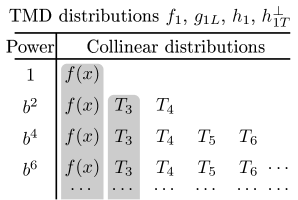
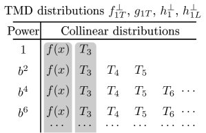
Figure 1: Ordering of parton distributions in the small-$b$ series for TMD distributions (3) (left) and (4) (right). $f(x)$ denotes the ordinary PDFs. $T_{n}$ denotes the parton distribution of twist-n, which is generally a function of several variables. The gray boxes designate the terms computed in this work.

To perform this computation, we use the technique inherited from Braun:2009vc ; Braun:2008ia , where it was used for the analyses of twist-4 operators. The technique is based on the local equivalence of the Lorentz transformation group to SL(2,C) group (so-called spinor formalism) Dreiner:2008tw . Within the spinor formalism, the twist-decomposition can be elegantly formulated as the action of a certain spinor-differential operator (see sec.3.2). In ref.Braun:2011dg this method has been used to derivate kinematic power corrections $(t/Q^{2})$ in deeply-virtual Compton scattering. In contrast to ref.Braun:2011dg , TMD operators are essentially non-local. They contain the gauge link along a staple contour. To overcome this difficulty, we introduce a formal local expansion for the TMD operator. To our best knowledge, it is the first time when the series of local operators successfully describes the infinite staple contours. Almost all expressions presented in this article are novel. Only some of them, namely $b^{0}$- and $b^{1}$-terms, can be found in literature and agree with it. Additionally, we demonstrate that the series of corrections for the unpolarized TMDPDF $f_{1}$ can be derived differently using the results of ref.Balitsky:1987bk and agrees with it.

The article is organized as follows. In sec.2 we articulate all definitions used in our work. This is an important part because we deal with functions that do not have a common definition such as polarized distributions and PDFs of twist-3. In sec.2.3 we specify the conventions for the spinor formalism used in our work. Sec.3 is devoted to the detailed description of the computation method. It is split into three subsections in accordance with three principal stages of the computation:(1), (2) and (3,4). So, in sec.3.1 the expansion (1) of the TMD operator in the series of (local) collinear operators is described. In sec.3.2 we explain the method of the twist-decomposition and derive it for TMD operators (2), with results for twist-3 part presented in the appendix A. The particularities of the computation of matrix elements for twist-decomposed operators are given in sec.3.3. The result of the computation and the discussion are given in sec.4.

2 Definitions and conventions

In this work, we operate with eight TMD distributions, three collinear twist-2 distributions and four collinear twist-3 distributions. They essentially depend on the conventions related to P-odd structures, such as Levi-Civita tensor, $\gamma^{5}$, etc. An additional set of conventions is brought by the spinor formalism which is used for the twist-decomposition. There is no commonly accepted convention for all these subjects in the literature, e.g. compare conventions in refs.Bacchetta:2006tn ; Braun:2009mi ; Jaffe:1996zw ; Kang:2011mr ; Kanazawa:2015ajw ; Sohnius:1985qm ; Dreiner:2008tw ; Scimemi:2018mmi . Nicely, the final result is mostly independent on the conventions, because it is the relation between physical distributions. Nonetheless, these conventions play an important role in the intermediate steps. In order to structure the presentation we collect all used definitions and conventions in this section.

2.1 Definition of TMD distributions

The light-cone decomposition plays the central role. It is defined by two light-like vectors $n^{\mu}$ and $\bar{n}^{\mu}$ ($n^{2}=\bar{n}^{2}=0$, $(n\bar{n})=1$). We use the ordinary notation of vector decomposition

$$v^{\mu}=v^{+}\bar{n}^{\mu}+v^{-}n^{\mu}+v_{T}^{\mu},$$ (6)

where $v^{+}=(nv)$, $v^{-}=(\bar{n}v)$, and $v_{T}$ is the transverse component $(v_{T}n)=(v_{T}\bar{n})=0$. In what follows, the direction $\bar{n}^{\mu}$ is associated with the large-component of the hadron momentum $p^{\mu}$,

$$p^{\mu}=p^{+}\bar{n}^{\mu}+\frac{n^{\mu}}{2}\frac{M^{2}}{p^{+}},$$ (7)

where $M$ is the mass of the hadron ($p^{2}=M^{2}$). It is important, that the hadron’s momentum does not have a transverse component, which gives the physical definition of the transverse plane. The spin of the hadron is parameterized by the spin-vector $S^{\mu}$, ($S^{2}=-1$, $(pS)=0$). Its light-cone decomposition is

$$S^{\mu}=\lambda\frac{p^{+}}{M}\bar{n}^{\mu}-\lambda\frac{M}{2p^{+}}n^{\mu}+s_{T}^{\mu},$$ (8)

where the $\lambda$ is the helicity of the hadron, and $s_{T}^{\mu}$ is the transverse component of the spin, $s_{T}^{2}=\lambda^{2}-1$.

The generic quark TMDPDF is defined as

$$\Phi_{ij}(x,b) = \int\frac{dz}{2\pi}e^{-ixzp^{+}}$$

$$\langle p,S|\bar{q}_{j}\left(zn+b\right)[zn+b,\mp\infty n+b][\mp\infty n+b,\mp\infty n][\mp\infty n,0]q_{i}(0)\}|p,S\rangle,$$

where the vector $b^{\mu}$ is a transverse vector, $(bp)=0$. The Wilson lines in the definition (2.1) are straight Wilson lines. Rigorously, one should add the T- and anti-T-ordering within the TMD operator. However, for the parton distributions (in contrast to fragmentation functions) it can be safely omitted (see e.g. discussion in Scimemi:2019gge ). TMDPDFs that appear in different processes have Wilson lines pointing into different direction, which is indicated by $\mp\infty n$ in (2.1). So, the TMD distributions which appear in semi-inclusive deep-inelastic scattering (SIDIS) have Wilson lines pointing to $+\infty n$, while in Drell-Yan they point to $-\infty n$. In the following, we distinguish these cases, and the upper sign refers to the Drell-Yan case, whereas the lower sign refers the SIDIS case.

The open indices $(ij)$ of the TMD operator in eq. (2.1) are to be contracted with different gamma-matrices, which we denote generically as $\Gamma$,

$$\Phi^{[\Gamma]} = \frac{1}{2}\mathrm{Tr}\left(\Phi\Gamma\right).$$ (10)

There are only three Dirac structures that appear in the leading term of the TMD factorization theorem, these are $\Gamma=\{\gamma^{+},\gamma^{+}\gamma_{5},i\sigma^{\alpha+}\gamma_{5}\}$. Here, the index $\alpha$ is transverse and

$$\sigma^{\mu\nu}=\frac{i}{2}(\gamma^{\mu}\gamma^{\nu}-\gamma^{\nu}\gamma^{\mu}),\qquad\gamma_{5}=i\gamma^{0}\gamma^{1}\gamma^{2}\gamma^{3}=\frac{-i}{4!}\epsilon_{\mu\nu\alpha\beta}\gamma^{\mu}\gamma^{\nu}\gamma^{\alpha}\gamma^{\beta},$$ (11)

with $\epsilon^{0123}=-\epsilon_{0123}=1$. In the naive parton model interpretation, these gamma-structures are related to the observation of unpolarized ($\gamma^{+}$), longitudinally polarized ($\gamma^{+}\gamma^{5}$) and transversely polarized ($i\sigma^{\alpha+}_{T}\gamma^{5}$) quarks inside the hadron. The standard parameterization of leading TMDPDFs in the position space reads

$$\Phi^{[\gamma^{+}]}(x,b) = f_{1}(x,b)+i\epsilon_{T}^{\mu\nu}b_{\mu}s_{T\nu}Mf_{1T}^{\perp}(x,b),$$ (12)

$$\Phi^{[\gamma^{+}\gamma_{5}]}(x,b) = \lambda g_{1L}(x,b)+ib_{\mu}s^{\mu}_{T}Mg_{1T}(x,b),$$ (13)

$$\Phi^{[i\sigma^{\alpha+}\gamma_{5}]}(x,b) = s_{T}^{\alpha}h_{1}(x,b)-i\lambda b^{\alpha}Mh_{1L}^{\perp}(x,b)$$ (14)

$$+i\epsilon_{T}^{\alpha\mu}b_{\mu}Mh_{1}^{\perp}(x,b)-\frac{M^{2}b^{2}}{2}\left(\frac{g_{T}^{\alpha\mu}}{2}-\frac{b^{\alpha}b^{\mu}}{b^{2}}\right)s_{T\mu}h_{1T}^{\perp}(x,b).$$

The tensors $g_{T}^{\mu\nu}$ and $\epsilon_{T}^{\mu\nu}$ are defined as

$$g_{T}^{\mu\nu}=g^{\mu\nu}-n^{\mu}\bar{n}^{\nu}-\bar{n}^{\mu}n^{\nu},\qquad\epsilon_{T}^{\mu\nu}=\epsilon^{-+\mu\nu},$$ (15)

such that $g_{T}^{11}=g_{T}^{22}=-1$, $\epsilon^{12}_{T}=-\epsilon^{21}_{T}=1$, and the rest components are zero. The definition of the TMDPDFs coincides with the conventional one in Scimemi:2018mmi ; Boer:2011xd ; Bacchetta:2006tn . In the following, we also compare to refs.Braun:2009mi ; Braun:2008ia ; Braun:2011dg , where the definitions of $\epsilon$ and $s_{T}$ have opposite sign, and ref.Scimemi:2018mmi , where the definition of $\epsilon$ and $\epsilon_{T}$ has opposite sign (so, component-wise the tensor $\epsilon^{\mu\nu}_{T}$ is the same). TMDPDFs defined in (12-14) are dimensionless functions which depend only on the modulus of $b$, but not on the direction. The conventional names for them are (see e.g.Boer:2011xd ; Bacchetta:2006tn ): unpolarized ($f_{1}$), Sivers ($f_{1T}^{\perp}$), helicity ($g_{1L}$), worm-gear T ($g_{1T}$), transversity $(h_{1})$, worm-gear L ($h_{1L}^{\perp}$), Boer-Mulders ($h_{1}^{\perp}$) and pretzelosity ($h_{1T}^{\perp}$) distributions.

The position space representation of TMD distribution is advantageous, because the TMD evolution is multiplicative in the position space. For that reason, the phenomenological studies that incorporate the TMD evolution are made in the position space, for the most recent examples see Scimemi:2019cmh ; Bacchetta:2019sam . TMD distributions in the momentum space are obtained by the Fourier transformation

$$\Phi^{[\Gamma]}(x,p_{T})=\int\frac{d^{2}b}{(2\pi)^{2}}e^{-i(bp_{T})}\Phi^{[\Gamma]}(x,b).$$ (16)

The transformation rules for particular TMD distributions can be found in refs.Boer:2011xd ; Scimemi:2018mmi .

2.2 Definition of collinear distributions

The collinear distributions of twist-2 are defined as Jaffe:1996zw

$$\langle p,S|\bar{q}(zn)[zn,0]\gamma^{+}q(0)|p,S\rangle = 2p^{+}\int dxe^{ixzp^{+}}f_{1}(x),$$ (17)

$$\langle p,S|\bar{q}(zn)[zn,0]\gamma^{+}\gamma^{5}q(0)|p,S\rangle = 2\lambda p^{+}\int dxe^{ixzp^{+}}g_{1}(x),$$ (18)

$$\langle p,S|\bar{q}(zn)[zn,0]\gamma^{+}i\sigma^{\alpha+}\gamma^{5}q(0)|p,S\rangle = 2s_{T}^{\alpha}p^{+}\int dxe^{ixzp^{+}}h_{1}(x),$$ (19)

where index $\alpha$ is transverse. These distributions are known as unpolarized $(f_{1})$, helicity $(g_{1})$ and transversity $(h_{1})$ PDFs. The variable $x$ belongs to the range $[-1,1]$ and for $x>0$ ($x<0$) PDFs are interpreted as probability densities for (anti-)quarks.

There is no conventional definition of the collinear distributions of twist-3. Here, we use the definition used in Scimemi:2018mmi . We define

$$\langle p,S|g\bar{q}(z_{1}n)F^{\mu+}(z_{2}n)\gamma^{+}q(z_{3}n)|p,S\rangle$$ (20)

$$\qquad\qquad\qquad=2\epsilon_{T}^{\mu\nu}s_{\nu T}(p^{+})^{2}M\int[dx]e^{-ip^{+}(z_{1}x_{1}+x_{2}z_{2}+x_{3}z_{3})}T(x_{1},x_{2},x_{3}),$$

$$\langle p,S|g\bar{q}(z_{1}n)F^{\mu+}(z_{2}n)\gamma^{+}\gamma^{5}q(z_{3}n)|p,S\rangle$$ (21)

$$\qquad\qquad\qquad=2is^{\mu}_{T}(p^{+})^{2}M\int[dx]e^{-ip^{+}(z_{1}x_{1}+x_{2}z_{2}+x_{3}z_{3})}\Delta T(x_{1},x_{2},x_{3}),$$

$$\langle p,S|g\bar{q}(z_{1}n)F^{\mu+}(z_{2}n)i\sigma^{\alpha+}\gamma^{5}q(z_{3}n)|p,S\rangle$$ (22)

$$\qquad\qquad\qquad=2\epsilon_{T}^{\mu\alpha}(p^{+})^{2}M\int[dx]e^{-ip^{+}(z_{1}x_{1}+x_{2}z_{2}+x_{3}z_{3})}\delta T_{\epsilon}(x_{1},x_{2},x_{3})$$

$$\qquad\qquad\qquad\qquad+2i\lambda g_{T}^{\mu\alpha}(p^{+})^{2}M\int[dx]e^{-ip^{+}(z_{1}x_{1}+x_{2}z_{2}+x_{3}z_{3})}\delta T_{g}(x_{1},x_{2},x_{3}),$$

where we omit Wilson lines that connect the fields in operators for brevity. The definition of the distributions $T$ and $\Delta T$ coincides with Scimemi:2018xaf and Braun:2009mi , taking into account the difference in conventions for the $\epsilon$-tensor (explained after (15)). In ref.Scimemi:2018xaf one can also find comparison with other definitions. The integration measure $[dx]$ is defined as

$$\int[dx]=\int_{-1}^{1}dx_{1}dx_{2}dx_{3}\delta(x_{1}+x_{2}+x_{3}).$$ (23)

The delta-function in this measure reflects the independence of the matrix element on the global position $(z_{1}+z_{2}+z_{3})$ of the field operator. Due to the delta-function in the measure, the distributions of twist-3 effectively depends on only two variables. Nonetheless, it is convenient to keep all three variables $x_{1,2,3}$ as independent. It reveals the symmetric properties Scimemi:2018mmi

$$T(x_{1},x_{2},x_{3}) = T(-x_{3},-x_{2},-x_{1}),\qquad\Delta T(x_{1},x_{2},x_{3})=-\Delta T(-x_{3},-x_{2},-x_{1}),$$ (24)

$$\delta T_{\epsilon}(x_{1},x_{2},x_{3}) = \delta T_{\epsilon}(-x_{3},-x_{2},-x_{1}),\qquad\delta T_{g}(x_{1},x_{2},x_{3})=-\delta T_{g}(-x_{3},-x_{2},-x_{1}).$$ (25)

Each range of $x_{1,2,3}\lessgtr 0$ has a specific partonic interpretation Jaffe:1996zw .

2.3 Spinor formalism

The twist-decomposition for local operators consists in the decomposition of tensors with many indices into irreducible representations of the Lorentz group SO(3,1). This procedure is greatly simplified in the spinor formalism. The spinor formalism is used in many parts of quantum field theory, for a review see Sohnius:1985qm ; Dreiner:2008tw . Here we remind only of the essential properties and introduce conventions that are necessary for the current work.

The spinor formalism is grounded on the local isomorphism of the Lorentz group to the group of complex unimodular matrices SL(2,C). The isomorphism is realized by the map of a four-vector to a hermitian matrix by the rule

$$x_{\alpha\dot{\alpha}}=x_{\mu}\sigma_{\alpha\dot{\alpha}}^{\mu},$$ (26)

where $\sigma^{\mu}=\{1,\sigma^{1},\sigma^{2},\sigma^{3}\}$ with $\sigma^{i}$ being the Pauli matrix. The scalar product of any two vectors is $x_{\mu}y^{\mu}=x_{\alpha\dot{\alpha}}y^{\dot{\alpha}\alpha}/2$. In the spinor formulation one must distinguish dotted and undotted indices because they are related to conjugated representations, $(u_{\alpha})^{*}=\bar{u}_{\dot{\alpha}}$. The scalar product of two spinors is defined as

$$(uv)=-u^{\alpha}v^{\beta}\epsilon_{\alpha\beta}=-(vu),\qquad(\bar{u}\bar{v})=-\bar{u}_{\dot{\alpha}}\bar{v}_{\dot{\beta}}\epsilon^{\dot{\alpha}\dot{\beta}}=-(\bar{v}\bar{u}),$$ (27)

where $\epsilon_{12}=-\epsilon_{\dot{1}\dot{2}}=1$ as in ref.Braun:2011dg ; Braun:2009vc ; Braun:2008ia .

The light-like vectors $n$ and $\bar{n}$ in the spinor formalism can be written as

$$n_{\alpha\dot{\alpha}}=\lambda_{\alpha}\bar{\lambda}_{\dot{\alpha}},\qquad\bar{n}_{\alpha\dot{\alpha}}=\mu_{\alpha}\bar{\mu}_{\dot{\alpha}},$$ (28)

where $\lambda$ and $\mu$ are independent spinors normalized as $(\bar{\lambda}\bar{\mu})(\mu\lambda)=2$. The spinors $\lambda$ and $\mu$ form the basis, which can be used to decompose any tensor. In particular, the decomposition (6) for an arbitrary four-vector is

$$x_{\alpha\dot{\alpha}}=\lambda_{\alpha}\bar{\lambda}_{\dot{\alpha}}x^{-}+\mu_{\alpha}\bar{\mu}_{\dot{\alpha}}x^{+}-\lambda_{\alpha}\bar{\mu}_{\dot{\alpha}}x_{T}-\mu_{\alpha}\bar{\lambda}_{\dot{\alpha}}\bar{x}_{T},$$ (29)

where $x_{T}$ and $\bar{x}_{T}$ are transverse components, $-2x_{T}\bar{x}_{T}=g_{T}^{\mu\nu}x_{\mu}x_{\nu}<0$.

The Dirac bi-spinors are written as composition of two-component spinors

$$\bar{q}=\left(\chi^{\beta},\bar{\psi}_{\dot{\alpha}}\right),\qquad q=\left(\begin{array}[]{c}\psi_{\alpha}\\ \bar{\chi}^{\dot{\beta}}\end{array}\right).$$ (32)

The decomposition of these spinors in the basis (28) is

$$\psi_{\alpha}=\frac{\lambda_{\alpha}\psi_{-}-\mu_{\alpha}\psi_{+}}{(\mu\lambda)},\qquad\bar{\psi}_{\dot{\alpha}}=\frac{\bar{\lambda}_{\dot{\alpha}}\bar{\psi}_{-}-\bar{\mu}_{\dot{\alpha}}\bar{\psi}_{+}}{(\bar{\lambda}\bar{\mu})},$$ (33)

where $\psi_{+}=(\lambda\psi)$, $\psi_{-}=(\mu\psi)$, etc. In the similar way we write down the decomposition of the gluon-strength tensor,

$$F_{\alpha\dot{\alpha},\beta\dot{\beta}}=2(f_{\alpha\beta}\epsilon_{\dot{\alpha}\dot{\beta}}-\epsilon_{\alpha\beta}\bar{f}_{\dot{\alpha}\dot{\beta}}),$$ (34)

where $f_{\alpha\beta}$ and $\bar{f}_{\dot{\alpha}\dot{\beta}}$ are symmetric tensors, $\bar{f}=f^{\dagger}$. In our computation we face only the gluon strength-tensor with one index transverse, and another contracted with the vector $n$. The decomposition of such tensor is

$$F_{\alpha\dot{\alpha},+}=\lambda_{\alpha}\bar{\lambda}_{\dot{\alpha}}\left(\frac{f_{+-}}{(\mu\lambda)}+\frac{\bar{f}_{+-}}{(\bar{\lambda}\bar{\mu})}\right)-\mu_{\alpha}\bar{\lambda}_{\dot{\alpha}}\frac{f_{++}}{(\mu\lambda)}-\lambda_{\alpha}\bar{\mu}_{\dot{\alpha}}\frac{\bar{f}_{++}}{(\bar{\lambda}\bar{\mu})},$$ (35)

where $f_{++}=f_{\alpha\beta}\lambda^{\alpha}\lambda^{\beta}$, $f_{+-}=f_{\alpha\beta}\lambda^{\alpha}\mu^{\beta}$, etc. The first term in (35) corresponds to $F_{-+}$ components, whereas the last two terms describe $F_{\mu+}$ with $\mu$ being transverse index.

Using the definitions (32) and (33) we write down the decompositions for the bi-spinor combinations. They are

$$\bar{q}\gamma^{+}q=\bar{\psi}_{+}\psi_{+}+\chi_{+}\bar{\chi}_{+},\qquad\bar{q}\gamma^{+}\gamma^{5}q=-\bar{\psi}_{+}\psi_{+}+\chi_{+}\bar{\chi}_{+},$$ (36)

$$\bar{q}i\sigma^{(\alpha\dot{\alpha})+}\gamma^{5}q=-2\left(\frac{\mu^{\alpha}\bar{\lambda}^{\dot{\alpha}}}{(\mu\lambda)}\chi_{+}\psi_{+}+\frac{\lambda^{\alpha}\bar{\mu}^{\dot{\alpha}}}{(\bar{\lambda}\bar{\mu})}\bar{\psi}_{+}\bar{\chi}_{+}\right),$$ (37)

where the order of the fields on LHS and RHS is preserved. Let us note that only “plus” components of quark fields appear in these decompositions. It is not accidental, but is the part of definition for the leading power TMD distributions. The components $\psi_{+}$, $\chi_{+}$, etc, are known as “good” components of quark field in contrast to “bad” components ($\psi_{-}$, $\chi_{-}$, etc) Jaffe:1996zw . The operators build only from good components (including also good components of the gluon field $f_{++}$ and $\bar{f}_{++}$) are called quasi-partonic operators. Their geometrical twist coincides with the collinear twist. All operators of twist-2 and twist-3 can be expressed as quasi-partonic operators with the help of EOMs Balitsky:1987bk .

The last ingredient needed for our computation are the equations of motion (EOMs) for the quark field  $\not{\!\!}\!Dq=0$ (for massless quarks). In the spinor notation EOMs are $D^{\dot{\alpha}\alpha}\psi_{\alpha}=0$, $\chi^{\alpha}\overleftarrow{D}_{\alpha\dot{\alpha}}=0$, similar for other spinors. Contracting these equations with basis spinors one receives EOMs for particular components. For our purposes we need the following EOMs

$$D_{\lambda\bar{\lambda}}\psi_{-}=D_{\mu\bar{\lambda}}\psi_{+},\qquad D_{\lambda\bar{\lambda}}\bar{\chi}_{-}=D_{\lambda\bar{\mu}}\bar{\chi}_{+},$$ (38)

$$\bar{\psi}_{-}\overleftarrow{D_{\lambda\bar{\lambda}}}=\bar{\psi}_{+}\overleftarrow{D_{\lambda\bar{\mu}}},\qquad\chi_{-}\overleftarrow{D_{\lambda\bar{\lambda}}}=\chi_{+}\overleftarrow{D_{\mu\bar{\lambda}}},$$ (39)

where $D_{ab}=D_{\alpha\dot{\alpha}}a^{\alpha}b^{\dot{\alpha}}$.

3 Twist-decomposition for TMD operators

In this section, we present details of the twist-decomposition procedure. The base of the method is taken from refs.Braun:2009vc ; Braun:2008ia , to which we refer for extended details and the theory foundation. There are three principal steps of the computation:

• The operator is presented as a series of local operators.

• Local operators are sorted by irreducible representation of Lorentz group (twists), and simplified using EOMs.

• The series of operators with the same twists are summed back into the non-local form.

This is a rather traditional approach for twist-decomposition. Examples of such consideration for collinear operators can be found in refs.Jaffe:1996zw ; Braun:2009vc ; Braun:2008ia ; Balitsky:1987bk ; Geyer:1999uq ; Belitsky:2000vx . For TMD operators each of these steps has a certain particularity. Let us list these particularities, and explain the methods that were used to resolve them:

• The TMD operator has infinite Wilson lines. Therefore, it is not possible to present it as the series of local operators directly. We regularize the TMD operator by truncation of the length of Wilson lines by the parameter $L$. Then TMD operators can be presented as a limit of triple series of local operators (50).

• The local operators for TMDPDFs have three sets of indices $(s,n,t)$. They correspond to the number of light-cone derivatives acting on $\bar{q}(s)$, the number of transverse derivatives ($n$) and the number of light-cone derivatives acting on $q(t$). Such structure somewhat complicates the twist-decomposition algebra, in comparison to the case of local operators that describe (Mellin moments of) collinear distributions, where all indices are alike. To simplify the twist-decomposition procedure we use the method introduced in refs.Braun:2008ia ; Braun:2009vc , which is based on the spinor formalism. This method allows to perform the twist-decomposition for the most general operators using only differential operations (compare to refs.Scimemi:2018mmi ; Ball:1998sk where off-light-cone generalizations of operators and integral equations are used, ref.Balitsky:1987bk where the differential equation are used, refs.Geyer:1999uq ; Belitsky:2000vx where an explicit procedure of index symmetrization is performed).

• The summation of the series is made for the matrix-elements, i.e. for distributions. It simplifies certain steps of computation, and helps to resolve potential ambiguities in the limit $L\to\infty$.

The following sections give details for each step in the order. The results of the computation are collected in the sec.4. We stress that such an approach is suitable only for TMDPDFs, but does not apply for TMDFF. The discussion for TMDFFs case is given in sec.B.

3.1 TMD operator as a series of local operators

Let us introduce the TMD operator in the form

$$O_{\text{TMD}}^{\Gamma}(z,b)=\bar{q}(zn+b)[zn+b,\mp\infty n+b][\mp\infty b+b,\mp\infty n]\Gamma[\mp\infty n,0]q(0).$$ (40)

The upper(lower) sign corresponds to Drell-Yan(SIDIS) induced TMD. The transverse gauge link $[\mp\infty n+b,\mp\infty n]$ ensures the explicit gauge invariance of the operator.

At the tree-order quantum fields can be treated as classical fields, and thus the small-$b$ expansion is an ordinary Taylor expansion. It is convenient to write it in the form (1)

$$O_{\text{TMD}}^{\Gamma}(z,b) = \sum_{n=0}^{\infty}\frac{b^{\mu_{1}}...b^{\mu_{n}}}{n!}\mathbb{O}^{\Gamma}_{\mu_{1}...\mu_{n}}(z),$$ (41)

with

$$\mathbb{O}^{\Gamma}_{\mu_{1}...\mu_{n}}(z)=\bar{q}(zn)[zn,-\infty n]\overleftarrow{D_{\mu_{1}}}...\overleftarrow{D_{\mu_{n}}}\Gamma[-\infty n,0]q(0),$$ (42)

where $D_{\mu}$ is the covariant derivative

$$\overleftarrow{D_{\mu}}=\partial_{\mu}+igA_{\mu},\qquad\overrightarrow{D_{\mu}}=\partial_{\mu}-igA_{\mu}.$$ (43)

The operators on RHS of (41) have collinear twist $n+2$, which follows from their dimension. At the same time, these operators do not have a definite geometrical twist, and therefore, their matrix element is a complicated composition of collinear distributions with different properties. Our goal is to perform the twist-decomposition and express these operators in terms of operators with definite geometrical twist.

In contrast to collinear operators, the TMD operator (40) spans the infinite range along the light cone. It is the most famous feature of TMD operators, and it leads to many physical effects, such as rapidity divergences Vladimirov:2017ksc , double-scale nature of TMD evolution Scimemi:2018xaf and the sign-change of P-odd distributions Collins:2002kn . In the $b\to 0$ limit, the infinite Wilson lines are partially compensated, due to the transitivity property of Wilson lines. For example, at $n=0$ the operator (42) simplifies to

$$\mathbb{O}^{\Gamma}(z)=\bar{q}(zn)[zn,-\infty n]\Gamma[-\infty n,0]q(0)=\bar{q}(zn)[zn,0]\Gamma q(0).$$ (44)

However, already at $n=1$ the infinities enter the expressions,

$$\mathbb{O}^{\Gamma}_{\mu}(z) = \bar{q}(z)\overleftarrow{D_{\mu}}[zn,0]q(0)+ig\int_{\mp\infty}^{z}d\sigma\bar{q}(zn)[zn,\tau n]F_{\mu+}(\tau n)[\tau n,0]q(0),$$ (45)

where $F_{\mu\nu}=ig^{-1}[D_{\mu},D_{\nu}]$ is the gluon-strength tensor. The operators on the RHS of these formulas are ordinary collinear operators. The infinite size of the TMD operator is reflected in the limit of integration in the last term of (45). In the form like (45), the twist-decomposition of operators is straightforward, although algebraically complicated Scimemi:2018mmi . The main reason of the complication is that each next order of expansion introduces new classes of operators, for instance at $n=2$ the operators like $\bar{q}(zn)F_{+\mu}(\tau_{1}n)F_{+\nu}(\tau_{2}n)q(0)$ and $\bar{q}(zn)[D_{\nu}F_{\mu+}(\tau n)]q(0)$ appear. Each of these new classes requires individual investigation, and therefore, this approach is ineffective.

To avoid these complications we operate directly with the operators (41) with the help of the following formal procedure. We introduce the regularized operator,

$$O_{\text{TMD}}^{\Gamma}(z,b;L)=\bar{q}(zn+b)[zn+b,Ln+b][Ln+b,Ln]\Gamma[Ln,0]q(0).$$ (46)

This operator turns to the TMD operator in the limit $L\to\mp\infty$. Note, that the same regularization also regularizes rapidity divergences and can be used used to derive the non-perturbative definition of the Collins-Soper kernel Vladimirov:2020umg . In the regularized form the operator (42) is

$$\mathbb{O}^{\Gamma}_{\mu_{1}...\mu_{n}}(z;L)=\bar{q}(zn)[zn,Ln]\overleftarrow{D_{\mu_{1}}}...\overleftarrow{D_{\mu_{n}}}\Gamma[Ln,0]q(0).$$ (47)

This operator can be written as the formal expansion,

$$\mathbb{O}^{\Gamma}_{\mu_{1}...\mu_{n}}(z;L)=\sum_{s,t=0}^{\infty}\frac{z_{1}^{s}z_{2}^{t}}{s!t!}\bar{q}\overleftarrow{D_{+}}^{s}\overleftarrow{D_{\mu_{1}}}...\overleftarrow{D_{\mu_{n}}}\Gamma\overrightarrow{D_{+}}^{t}q(Ln),$$ (48)

where

$$z_{1}=z-L,\qquad z_{2}=-L.$$ (49)

In this way the TMD operator (40) is presented as a triple sum

$$O_{\text{TMD}}^{\Gamma}(z;b)=\lim_{L\to\mp\infty}\sum_{s,t,n=0}^{\infty}\frac{z_{1}^{s}}{s!}\frac{z_{2}^{t}}{t!}\frac{1}{n!}O^{\Gamma}_{s,n,t}(Ln),$$ (50)

with

$$O^{\Gamma}_{s,n,t} = \bar{q}\overleftarrow{D_{+}}^{s}(b\cdot\overleftarrow{D})^{n}\Gamma\overrightarrow{D_{+}}^{t}q.$$ (51)

The RHS of this expression is suitable for the twist-decomposition procedure.

The limit $L\to\mp\infty$ must be taken with caution. In particular, the summation over $s$ and $t$ must be done before the limiting operation, and the result of the summation should be presented in the form that does not allow any ambiguity. The significant simplification of the summation procedure comes from the possibility to neglect the total derivative terms. The matrix element of a total-derivative operator is proportional to the momentum transfer,

$$\langle p_{1}|\partial_{\mu}O|p_{2}\rangle=i(p_{1}-p_{2})_{\mu}\langle p_{1}|O|p_{2}\rangle.$$ (52)

Consequently, the total derivative operators do not contribute to TMDPDFs, and we neglect such terms in the following. After elimination of the total derivative contribution the result of summation is independent on $L$ in many cases. The simplest example is $n=0$ case, where

$$\sum_{s,t=0}^{\infty}\frac{z_{1}^{s}}{s!}\frac{z_{2}^{t}}{t!}O^{\Gamma}_{s,0,t} = \sum_{s,t=0}^{\infty}\frac{z_{1}^{s}}{s!}\frac{(-z_{2})^{t}}{t!}O^{\Gamma}_{s+t,0,0}+\text{total der.}$$

$$= \sum_{s=0}^{\infty}\frac{(z_{1}-z_{2})^{s}}{s!}O^{\Gamma}_{s,0,0}+\text{total der.}~{},$$

with $z_{1}-z_{2}=z$ being independent on $L$. Only in the cases of Sivers and Boer-Mulders functions the limit $L\to\mp\infty$ is not so straightforward. Let us also note that the direction of the limit is the only difference between Drell-Yan $(L\to-\infty)$ and SIDIS $(L\to+\infty)$ cases in the representation (50).

3.2 Twist decomposition in the spinor formalism

The twist-decomposition for the local operators (51) is equivalent to the decomposition into irreducible representation of Lorentz group. The highest spin representation (completely symmetric and traceless in all vector indices) corresponds to the twist-2 term. The next representation (anti-symmetric for one pair of indices, and symmetric and traceless for all other vector indices) corresponds to twist-3 term. Despite the twist-decomposition is a straightforward operation, it is algebraically complicated, especially for the operators with many transverse indices (for which one has to subtract traces). Additional complication is caused by EOMs, which could relate operators. In refs.Braun:2009vc ; Braun:2008ia it was observed that the decomposition of higher-indices tensors over irreducible representations is simpler in the spinor representation. The main simplification comes from the anti-symmetry of the scalar product (27). Due to it, any symmetric tensor (in the spinor space) is automatically traceless. The irreducible representations in SL(2,C) group are obtained by simple symmetrization or anti-symmetrization of spinor indices. This operation can be presented as a differential operator, what essentially simplifies the algebra. Here we present this methods in a slightly modified form, which makes its application more explicit.

Let us consider an operator where all open indices are contracted with basis spinors:

$$\mathbb{O}_{\Lambda}=\Lambda_{1}^{\alpha...\beta}(\lambda,\mu)\Lambda_{2}^{\dot{\alpha}...\dot{\beta}}(\bar{\lambda},\bar{\mu})\mathbb{O}_{\alpha...\beta;\dot{\alpha}...\dot{\beta}},$$ (54)

where $\Lambda_{1,2}$ are monomials of basis spinors, for example (66). The lowest geometrical twist contribution can be obtained by the symmetrization of dotted and undotted indices (independently). It can be done for the operator, or for the tensor $\Lambda$. Due to the irreducibility of the representation the symmetry properties of one are mapped to another in the convolution. The symmetrization of the tensor $\Lambda$ can be made by the following operation

$$S_{n}\Lambda^{\alpha...\beta}(\lambda,\mu)=\left(\frac{\mu\partial}{\partial\lambda}\right)^{n}\left(\frac{\lambda\partial}{\partial\mu}\right)^{n}\Lambda^{\alpha...\beta}(\lambda,\mu),$$ (55)

where

$$\frac{\mu\partial}{\partial\lambda}=\mu^{\alpha}\frac{\partial}{\partial\lambda^{\alpha}},\qquad\frac{\lambda\partial}{\partial\mu}=\lambda^{\alpha}\frac{\partial}{\partial\mu^{\alpha}},$$ (56)

and $n$ is the number of spinors $\mu$ in the tensor $\Lambda$. The logic behind the construction is the following. First, the action of derivatives $(\lambda\partial)/(\partial\mu)$ replaces all $\mu$’s by $\lambda$’s. The resulting tensor is automatically symmetric in indices. Next, the derivatives $(\mu\partial)/(\partial\lambda)$ replace entries of $\lambda$ by $\mu$ in the fully symmetric fashion.

The higher twist representations are build by anti-symmetrizing pairs of indices. So, the anti-symmetrization of a single pair can be done by the operator

$$A_{1}=(\mu^{\alpha}\lambda^{\beta}-\lambda^{\alpha}\mu^{\beta})\frac{\partial}{\partial\mu^{\alpha}}\frac{\partial}{\partial\lambda^{\beta}}=\frac{\mu\partial}{\partial\mu}\frac{\lambda\partial}{\partial\lambda}-\frac{\mu\partial}{\partial\lambda}\frac{\lambda\partial}{\partial\mu}+\frac{\mu\partial}{\partial\mu},$$ (57)

where $(\mu\partial)/(\partial\mu)$ and $(\lambda\partial)/(\partial\lambda)$ defined similarly to (56). The symmetrization of $n$ pairs is done by

$$A_{n}=(\mu^{\alpha_{1}}\lambda^{\beta_{1}}-\lambda^{\alpha_{1}}\mu^{\beta_{1}})...(\mu^{\alpha_{n}}\lambda^{\beta_{n}}-\lambda^{\alpha_{n}}\mu^{\beta_{n}})\frac{\partial}{\partial\mu^{\alpha_{1}}}\frac{\partial}{\partial\lambda^{\beta_{1}}}...\frac{\partial}{\partial\mu^{\alpha_{n}}}\frac{\partial}{\partial\lambda^{\beta_{n}}}.$$ (58)

The operators $S$ and $A$ commute, $[A_{n},S_{k}]=0$, for any $n$ and $k$. The complete decomposition of a tensor with $n$ entries of spinor $\mu$ then reads

$$\Lambda^{\alpha...\beta}(\lambda,\mu)=\sum_{k=0}^{n}c_{n,k}A_{k}S_{n-k}\Lambda^{\alpha...\beta}(\lambda,\mu),$$ (59)

where $c_{n,k}$ are numbers depending on the tensor $\Lambda$. Each term in this sum corresponds to an irreducible representation, and the operators $S_{n-k}A_{k}$ are projectors onto this representation.

To find the coefficients $c_{n,k}$ of the decompositions (59) we need to normalize the operators $A_{k}S_{n}$, such that $(A_{k}S_{n})^{2}=A_{k}S_{n}$. For example, for the symmetrization operator we compute

$$S_{n}S_{n}=n!S_{n}\prod_{m=0}^{n-1}\left(\frac{\lambda\partial}{\partial\lambda}+\frac{\mu\partial}{\partial\mu}-m\right).$$ (60)

The operators $(\lambda\partial)/(\partial\lambda)$ and $(\mu\partial)/(\partial\mu)$ count the number of $\lambda$’s and $\mu$’s in the tensor. Therefore, $S_{n}$ is indeed the projector to the totally symmetric representation, and the normalization factor for $S_{n}$ is $(N-n)!/(n!N!)$ where $N$ is the total number of indices of the tensor. In the same way, one can check that $A_{n}S_{k}$ are projectors, and find the corresponding normalization factors. For our computation we only need the first two terms of the expansion (59). They are

$$\Lambda^{\alpha...\beta}(\lambda,\mu)=\left(\frac{(N-n)!}{n!N!}S_{n}+\frac{(N-n-1)!(N-1)}{(n-1)!N!}A_{1}S_{n-1}+...\right)\Lambda^{\alpha...\beta}(\lambda,\mu),$$ (61)

where $N$ is the total number of indices, and $n$ is the number of $\mu$’s in the tensor $\Lambda$.

Using this construction we build the operators that extract a part with the certain geometrical twist from the operator (54)

$$O_{\Lambda}=\sum_{n=2}^{\infty}\hat{T}_{n}O_{\Lambda}.$$ (62)

The projectors to the twist-2 is

$$\hat{T}_{2}=\left(\frac{\mu\partial}{\partial\lambda}\right)^{n}\left(\frac{\bar{\mu}\partial}{\partial\bar{\lambda}}\right)^{k}\frac{(N-n)!}{n!N!}\frac{(\bar{N}-k)!}{k!\bar{N}!}\left(\frac{\lambda\partial}{\partial\mu}\right)^{n}\left(\frac{\bar{\lambda}\partial}{\partial\bar{\mu}}\right)^{k},$$ (63)

where $n$, $k$, $N-n$ and $\bar{N}-k$ are the numbers of $\mu$, $\bar{\mu}$, $\lambda$ and $\bar{\lambda}$ in the operator. The operator that projects the twist-3 has two terms

$$\hat{T}_{3}=T^{(\mu\lambda)}_{3}+\hat{T}^{(\bar{\mu}\bar{\lambda})}_{3},$$ (64)

where $\hat{T}^{(\mu\lambda)}_{3}$ anti-symmetrizes a pair $(\mu,\lambda)$, whereas $\hat{T}^{(\bar{\mu}\bar{\lambda})}_{3}$ anti-symmetrizes a pair $(\bar{\mu},\bar{\lambda})$. Explicitly $\hat{T}^{(\mu\lambda)}_{3}$ reads

$$\hat{T}^{(\mu\lambda)}_{3}=$$ (65)

$$\left(\frac{\mu\partial}{\partial\lambda}\right)^{n-1}\left(\frac{\bar{\mu}\partial}{\partial\bar{\lambda}}\right)^{k}\frac{(N-n-1)!(N-1)}{(n-1)!N!}\frac{(\bar{N}-k)!}{k!\bar{N}!}\left(\frac{\mu\partial}{\partial\mu}\frac{\lambda\partial}{\partial\lambda}-\frac{\mu\partial}{\partial\lambda}\frac{\lambda\partial}{\partial\mu}+\frac{\mu\partial}{\partial\mu}\right)\left(\frac{\lambda\partial}{\partial\mu}\right)^{n-1}\left(\frac{\bar{\lambda}\partial}{\partial\bar{\mu}}\right)^{k},$$

where $n$, $k$, $N-n$ and $\bar{N}-k$ are the numbers of $\mu$, $\bar{\mu}$, $\lambda$ and $\bar{\lambda}$ in the operator. The operator $\hat{T}^{(\bar{\mu}\bar{\lambda})}_{3}$ is obtained by the interchange of barred and un-barred variables.

In this way, the twist-decomposition is reduced to purely algebraic manipulations with monomials. One should distinguish the chiral-even (given in (36)) and chiral-odd (given in (37)) compositions of spinors, because they have different number of barred and un-barred spinors. Apart of this, the evaluation of all cases is alike. In the following we demonstrate the results of action by $T_{2}$ and $T_{3}$ on $O^{\Gamma}_{s,n,t}$. For simplicity of presentation, we replace the indication of the Dirac structure in $O^{\Gamma}_{s,n,t}$, by the indication of the corresponding spinor combination. Additionally, we write operators using spinor notation only. For example

$$O^{\bar{\psi}_{+}\psi_{+}}_{s,n,t} = \bar{\psi}_{+}\overleftarrow{D_{\lambda\bar{\lambda}}}^{s}(b\overleftarrow{D_{\lambda\bar{\mu}}}+\bar{b}\overleftarrow{D_{\mu\bar{\lambda}}})^{n}\overrightarrow{D_{\lambda\bar{\lambda}}}^{t}\psi_{+}=(-1)^{n}2^{s+t+n}\bar{\psi}_{+}\overleftarrow{D_{+}}^{s}(b\cdot\overleftarrow{D})^{n}\Gamma\overrightarrow{D_{+}}^{t}\psi_{+},$$ (66)

where the prefactor is originated from the conventions (27-29). Also we eliminate all total-derivative terms without indication.

The twist-2 part of the chiral-even operator is

$$\hat{T}_{2}O^{\bar{\psi}_{+}\psi_{+}}_{s,n,t}=$$ (67)

$$\qquad\sum_{k=0}^{n}\left(\frac{\mu\partial}{\partial\lambda}\right)^{n-k}\left(\frac{\bar{\mu}\partial}{\partial\bar{\lambda}}\right)^{k}\frac{(-1)^{t}n!}{k!(n-k)!}\frac{(s+t+k+1)!}{(s+t+n+1)!}\frac{(s+t+n-k+1)!}{(s+t+n+1)!}b^{k}\bar{b}^{n-k}\bar{\psi}_{+}\overleftarrow{D}_{\lambda\bar{\lambda}}^{s+t+n}\psi_{+},$$

and the same for ${\bar{\psi}_{+}\psi_{+}}\to{\chi_{+}\bar{\chi}_{+}}$. The twist-2 part of the chiral-odd operator is

$$\hat{T}_{2}O^{\chi_{+}\psi_{+}}_{s,n,t}=$$ (68)

$$\qquad\sum_{k=0}^{n}\left(\frac{\mu\partial}{\partial\lambda}\right)^{n-k}\left(\frac{\bar{\mu}\partial}{\partial\bar{\lambda}}\right)^{k}\frac{(-1)^{t}n!}{k!(n-k)!}\frac{(s+t+k+2)!}{(s+t+n+2)!}\frac{(s+t+n-k)!}{(s+t+n)!}b^{k}\bar{b}^{n-k}\chi_{+}\overleftarrow{D}_{\lambda\bar{\lambda}}^{s+t+n}\psi_{+},$$

and the same for ${\chi_{+}\psi_{+}}\to{\bar{\psi}_{+}\bar{\chi}_{+}}$. In equations (67,68) we leave the derivatives with respect $(\mu\partial)/(\partial\lambda)$ and $(\bar{\mu}\partial)/(\partial\bar{\lambda})$ without evaluation for future convenience. Note, that factor $(-1)^{t}$ is originated from reversing the derivative $\overrightarrow{D}^{t}$ to $\overleftarrow{D}^{t}$ and elimination of total derivatives.

The derivation of the twist-3 part is slightly more cumbersome, due to the reduction procedure to the quasi-partonic form. We remind that the quasi-partonic operators consist only of “good” components of fields and $D_{\lambda\bar{\lambda}}$. All twist-3 operators can be reduced to this form. The reduction procedure is done as follows. After the action of $A_{1}$ we obtain operators of the form $\bar{\psi}_{+}D_{\lambda\bar{\lambda}}^{N}D_{\lambda\bar{\mu}}D_{\lambda\bar{\lambda}}^{M}\psi_{+}$ and $\bar{\psi}_{-}D_{\lambda\bar{\lambda}}^{N}\psi_{+}$. Next, we commute the derivative with the transverse index to the quark field, such that it can be replaced by appropriate EOM (38). After this procedure all “bad” components of quark field cancel, and the twist-3 operator has the quasi-partonic form. The expressions for the twist-3 parts of operators are simple but rather lengthy. For example,

$$\hat{T}_{3}^{(\bar{\mu}\bar{\lambda})}O_{s,n,t}^{\bar{\psi}_{+}\psi_{+}} = 2ig\sum_{k=1}^{n}\left(\frac{\mu\partial}{\partial\lambda}\right)^{n-k}\left(\frac{\bar{\mu}\partial}{\partial\bar{\lambda}}\right)^{k-1}$$

$$\frac{(-1)^{t}(n-1)!}{(k-1)!(n-k)!}\frac{(s+t+n-k)!(s+t+n)}{(s+t+n+1)!}\frac{(s+t+k+1)!}{(s+t+n+1)!}$$

$$b^{k}\bar{b}^{n-k}(\bar{\lambda}\bar{\mu})\Bigg{\{}(s+t+n+1)n\sum_{m=0}^{s-2}+(s+t+n+1)\sum_{m=s-1}^{s+n-2}(s+n-m-1)$$

$$-n\sum_{m=0}^{s+t+n-2}(s+t+n-m-1)\Bigg{\}}\bar{\psi}_{+}\overleftarrow{D}_{\lambda\bar{\lambda}}^{m}f_{++}\overleftarrow{D}_{\lambda\bar{\lambda}}^{s+t+n-m-2}\psi_{+}.$$

Here, the summations over $m$ are originated from the commutation procedure. Other spinor combinations and action of $\hat{T}_{3}^{(\mu\lambda)}$ differ from this example by $\pm 1$ terms in the factorial factors and summation limits. For completeness these expressions are listed in the appendix A.

3.3 Assembling the final result

The last step of the computation is to sum the operators over $s$ and $t$ to the non-local form and perform the limit $L\to\infty$. This procedure can be done directly in terms of operators. However, the resulting expression has an overcomplicated form, because the most part of the expression vanishes on the level of matrix element due to symmetry relations (24,25). To avoid these complications we first compute the matrix element and then sum the expression. Conveniently, the evaluation of the matrix elements can be done before we apply the derivatives $(\mu\partial)/(\partial\lambda)$ and $(\bar{\mu}\partial)/(\partial\bar{\lambda})$, which then act on the parameterization of the matrix element. The process is identical for all distributions. Here we demonstrate the computation for the case $\Gamma=\gamma^{+}$ which contains unpolarized and Sivers TMD distributions. The peculiarities of the computation for other cases are discussed at the end of the section.

The matrix element for the twist-2 operator with $\Gamma=\gamma^{+}$ is expressed in the terms of unpolarized PDF (17) as (36)

$$\langle p,S|\bar{\psi}_{+}\overleftarrow{D}_{\lambda\bar{\lambda}}^{N}\psi_{+}+\chi_{+}\overleftarrow{D}_{\lambda\bar{\lambda}}^{N}\bar{\chi}_{+}|p,S\rangle=i^{N}p_{\lambda\bar{\lambda}}^{N+1}\int dxx^{N}f_{1}(x).$$ (70)

Substituting it into (67), we observe that the derivatives $(\mu\partial)/(\partial\lambda)$ and $(\bar{\mu}\partial)/(\partial\bar{\lambda})$ now could act only on $p_{\lambda\bar{\lambda}}$. At the same time, the vector $p^{\mu}$ does not have a transverse part (by definition), i.e. $p_{\lambda\bar{\mu}}=p_{\mu\bar{\lambda}}=0$, and thus only the terms with $n=2k$ are non-zero:

$$\left(\frac{\mu\partial}{\partial\lambda}\right)^{n-k}\left(\frac{\bar{\mu}\partial}{\partial\bar{\lambda}}\right)^{k}p_{\lambda\bar{\lambda}}^{s+t+n+1}=\delta_{n,2k}\frac{(s+t+n+1)!k!}{(s+t+n-k+1)!}p_{\lambda\bar{\lambda}}^{s+t+n-k+1}p_{\mu\bar{\mu}}^{k}.$$ (71)

Now, we can pass to the vector notation, and the expression for the matrix element takes the form

$$\langle p,S|\hat{T}_{2}O^{[\gamma^{+}]}(z,b)|p,S\rangle=$$ (72)

$$\qquad p^{+}\lim_{L\to\mp\infty}\sum_{n=0}^{\infty}\frac{1}{n!}\left(\frac{b^{2}M^{2}}{4}\right)^{n}\sum_{s,t=0}^{\infty}\frac{z_{1}^{s}z_{2}^{t}(ip^{+})^{s+t}}{s!t!}\frac{(s+t+n+1)!}{(s+t+2n+1)!}\int dxx^{s+t+2n}f_{1}(x),$$

where we used that $b\bar{b}=-b^{2}/2$, $p_{\lambda\bar{\lambda}}=2p^{+}$ and $p_{\mu\bar{\mu}}=2p^{-}=M^{2}/p^{+}$. Presenting the factorial factor by the beta-function (for $n>0$) we evaluate the sum over $s$ and $t$. The summation produces the exponent $\exp(i(z_{1}-z_{2})zp^{+})$ that is independent on $L$ due to (49). Therefore, in this case the limit $L\to\pm\infty$ is trivial. The summed expression reads

$$\langle p,S|T_{2}O^{[\gamma^{+}]}(z,b)|p,S\rangle=$$ (73)

$$\qquad p^{+}\int dxf_{1}(x)e^{izp_{+}x}+\int_{0}^{1}du\int dx\sum_{n=1}^{\infty}\frac{u^{n+1}\bar{u}^{n-1}x^{2n}}{n!(n-1)!}\left(\frac{b^{2}M^{2}}{4}\right)^{n}e^{iuzp_{+}x}f_{1}(x),$$

where $\bar{u}=1-u$. Finally, we make the inverse Fourier transformation and compare the result to the parameterization (12). We find that the twist-2 part of the operator contributes only to the unpolarized TMD distribution. The final expression is convenient to present in the form of Mellin convolution (96)

$$f_{1}(x,b)=f_{1}(x)+\sum_{n=1}^{\infty}\int_{0}^{1}du\int dy\frac{\delta(x-uy)}{n!(n-1)!}\left(\frac{\bar{u}}{u}\right)^{n-1}\left(\frac{x^{2}b^{2}M^{2}}{4}\right)^{n}f_{1}(y)+\mathcal{O}(\alpha_{s},\text{tw4}).$$ (74)

This is the complete part of the small-$b$ expansion for $f_{1}(x,b)$ that is matches twist-2 PDFs. The corrections to this expression contain PDFs of higher twist, starting from twist-4 (the absence of twist-3 part is demonstrated later). Also each term in this sum receives the perturbative corrections. All these corrections are indicated by $\mathcal{O}(\alpha_{s},\text{tw4})$.

The computation of the twist-3 part follows the same pattern, but involves more terms. We use the matrix elements (20,21), and present them in the form of double moments

$$\langle p,S|g\bar{\psi}_{+}\overleftarrow{D}^{N}_{\lambda\bar{\lambda}}f_{++}\overleftarrow{D}^{M}_{\lambda\bar{\lambda}}\psi_{+}|p,S\rangle=$$ (75)

$$\qquad(-i)^{N}i^{M}p_{\lambda\bar{\lambda}}^{N+M+2}\frac{-iS_{\lambda\bar{\mu}}}{2(\bar{\lambda}\bar{\mu})}\int[dx]x_{1}^{N}x_{3}^{M}\left(T(x_{1},x_{2},x_{3})+\Delta T(x_{1},x_{2},x_{3})\right),$$

and similarly for other spinor combinations. Now, the derivatives $(\mu\partial)/(\partial\lambda)$ and $(\bar{\mu}\partial)/(\partial\bar{\lambda})$ also act on the vector $S$, and thus the expression analogous to (71) contains two terms. One with $n=2k-1$ that is proportional to transverse part of $S$, and another one with $n=2k-2$ that is proportional to $S_{\mu\bar{\mu}}=-\lambda M/p^{+}$. The parts proportional to $\lambda$ add up to zero for $\Gamma=\gamma^{+}$, however, in the case of $\Gamma=\gamma^{+}\gamma^{5}$ they produce the twist-3 terms in the helicity TMD distribution $g_{1L}$. After these operations the summation over $m$ reduces to geometric progressions. The resulting expression is rather lengthy

$$\langle p,S|\hat{T}_{3}O^{[\gamma^{+}]}(z,b)|p,S\rangle=Mp^{+}(b_{\mu}\epsilon_{T}^{\mu\nu}S_{\nu})\lim_{L\to\mp\infty}\int[dx]\sum_{n=0}^{\infty}\frac{1}{(2n+1)n!}\left(\frac{b^{2}M^{2}}{4}\right)^{n}$$ (76)

$$\qquad\qquad\sum_{s,t=0}^{\infty}\frac{z_{1}^{s}z_{2}^{t}(ip^{+})^{s+t}}{s!t!}\frac{(s+t+n)!}{(s+t+2n+2)!}\frac{(s+t+2n+1)(s+t+n+2)}{(s+t+2n+2)}\Bigg{\{}$$

$$\qquad\qquad(2n+1)\left[(-x_{1})^{s}x_{1}^{t+2n+1}\left(2-\frac{x_{2}}{x_{1}}\right)+(-x_{3})^{t}x_{3}^{s+2n+1}\left(2-\frac{x_{2}}{x_{3}}\right)\right]\frac{T(x_{1},x_{2},x_{3})}{x_{2}^{2}}$$

$$\qquad\qquad-(2n+1)\left[(-x_{1})^{s}x_{1}^{t+2n}-(-x_{3})^{t}x_{3}^{s+2n}\right]\frac{\Delta T(x_{1},x_{2},x_{3})}{x_{2}}$$

$$\qquad\qquad-(s+t+2n+2)(-x_{1})^{s}(-x_{3})^{t}(x_{1}^{2n+1}+x_{3}^{2n+1})\frac{T(x_{1},x_{2},x_{3})}{x_{2}^{2}}\Bigg{\}},$$

where we have used that $x_{1}+x_{2}+x_{3}=0$ for simplifications. This expression is very representative and demonstrates many features of the computation. Notably, there are two types of contributions relative to the summation over $s$ and $t$. The regular ones that are in the third and forth lines, and the irregular one that is in the last line.

The regular contributions have a general form of (see also (3.1,72))

$$\sum_{s,t=0}^{\infty}\frac{z_{1}^{s}(-z_{2})^{t}}{s!t!}f(s+t)=\sum_{r=0}^{\infty}\frac{(z_{1}-z_{2})^{r}}{r!}f(r),$$ (77)

and are explicitly independent on $L$, since $z_{1}-z_{2}=z$ (49). For regular contributions, the limit $L\to\mp\infty$ is trivial, and the resulting operators are spatially compact. The final expression has ordinary form with twist-3 distributions, see eqns.(4,4,4,4,4). In the current example with $\Gamma=\gamma^{+}$, these term do not appear in the final expression, due to symmetry properties (24). Indeed, the change of variables $\{x_{1},x_{2},x_{3}\}\to\{-x_{3},-x_{2},-x_{1}\}$ flips the common sign of the prefactors in square brackets, but leaves $T/x_{2}^{2}$ and $\Delta T/x_{2}$ unchanged. Thus, the contribution of the third and the fourth lines vanishes.

The evaluation of irregular terms requires special attention. The sums over $s$ and $t$ lead to the following expression

$$\langle p,S|\hat{T}_{3}O^{[\gamma^{+}]}(z,b)|p,S\rangle=$$ (78)

$$\qquad\qquad-Mp^{+}(b_{\mu}\epsilon_{T}^{\mu\nu}S_{\nu})\lim_{L\to\mp\infty}\int_{0}^{1}du\int[dx]\sum_{n=0}^{\infty}\left(\frac{b^{2}M^{2}}{4}\right)^{n}e^{-iup^{+}(z_{1}x_{1}+z_{3}x_{3})}$$

$$\qquad\qquad\frac{(u\bar{u})^{n}}{(2n+1)n!}\left(\delta_{n,0}\delta(\bar{u})+\frac{n}{(n-1)!}\frac{1+(n-1)u+u^{2}}{\bar{u}}\right)(x_{1}^{2n+1}+x_{3}^{2n+1})\frac{T(x_{1},x_{2},x_{3})}{x_{2}^{2}}.$$

The limit $L\to\mp\infty$ is ill-defined, because $(z_{1}x_{1}+z_{3}x_{3})=(zx_{1}+Lx_{2})$. To resolve this ambiguity, we use the symmetry of the integration measure $[dx]$ and transfer the variable $L$ to the limits of the integration

$$\int[dx]e^{-iup^{+}(z_{1}x_{1}+z_{3}x_{3})}=(-ip^{+}u)\int[dx]x_{2}\,e^{-ip_{+}uzx_{1}}\int_{-L+z}^{L}d\tau\frac{e^{-ip_{+}u\tau x_{2}}}{2}.$$ (79)

Now, the limit can be taken, and the last integral in (79) is the delta-function

$$\lim_{L\to\mp\infty}(-ip^{+}u)\int_{-L+z}^{L}d\tau\frac{e^{-ip_{+}u\tau x_{2}}}{2}=\mp i\pi\delta(x_{2}).$$ (80)

It is important that the sign of this expression depends on the sign of the limiting direction. This is how the famous sign-flip for the Sivers function appears in this computation. To integrate over $x_{2}$, we extract all entries of $x_{2}$ in (79) with the help of relation

$$\frac{x_{1}^{2n+1}+x_{3}^{2n+1}}{x_{2}}=-\sum_{m=0}^{n}(-x_{1}x_{3})^{m}x_{2}^{2n-2m}\frac{(2n+1)(2n-m)!}{m!(2n-2m+1)!}.$$ (81)

Clearly, only the term with $m=0$ contributes. Performing the Fourier transformation and comparing it to (12) we conclude that it is the contribution to the Sivers function, which reads

$$f_{1T}^{\perp}(x,b) = \pm\pi\Big{[}T(-x,0,x)+\int_{0}^{1}du\int dy\sum_{n=1}^{\infty}\left(\frac{x^{2}b^{2}M^{2}}{4}\right)^{n}$$

$$\frac{\delta(x-uy)}{(n-1)!(n+1)!}\left(\frac{\bar{u}}{u}\right)^{n}\frac{1+(n-1)u+u^{2}}{\bar{u}}T(-y,0,y)+\mathcal{O}(\alpha_{s},\text{tw4})\Big{]}.$$

This is the matching of the Sivers function at all orders of $b^{2}$-expansion to collinear distributions of twist-2 (which is null) and twist-3. Miraculously, only the Qui-Sterman function $T(-x,0,x)$ Qiu:1991pp contributes to this expression. As expected, the sign of the Sivers function depends on the direction of the gauge contour.

The computation of other Lorentz structures is done in the same way. The differences to the demonstrated computation are immaterial. The resulting expression are not as simple as for $\Gamma=\gamma^{+}$ case. In particular, generally the distributions have entries of both twist-2 and twist-3 PDFs. It happens due to non-vanishing contributions with derivatives of the vector $S_{\mu}$. For example, for $\Gamma=\gamma^{+}\gamma^{5}$ the analog of (70) has $S_{\lambda\bar{\lambda}}$ which after the differentiation (71) produces the transverse components of $S$. These terms result into twist-2 PDFs within worm-gear function. In all P-even cases only regular terms contribute, whereas P-odd cases (i.e. Sivers and Boer-Mulders functions) are given by only irregular terms. The results of our computation together with additional comments are presented in the next section.

4 Results and discussion

Following the method derived in the previous section we routinely computed all (quark) TMD distributions. Here is the list of expressions. The chiral-even distributions are

$$f_{1}(x,b) = f_{1}(x)+\sum_{n=1}^{\infty}\int_{0}^{1}du\int dy\frac{\delta(x-uy)}{n!(n-1)!}\left(\frac{x^{2}b^{2}M^{2}}{4}\right)^{n}\left(\frac{\bar{u}}{u}\right)^{n-1}f_{1}(y),$$ (83)

$$f_{1T}^{\perp}(x,b) = \pm\pi\Big{[}T(-x,0,x)+\sum_{n=1}^{\infty}\left(\frac{x^{2}b^{2}M^{2}}{4}\right)^{n}\int_{0}^{1}du\int dy\frac{\delta(x-uy)}{(n+1)!(n-1)!}$$

$$\qquad\qquad\times\left(\frac{\bar{u}}{u}\right)^{n}\frac{1+(n-1)u+u^{2}}{\bar{u}}T(-y,0,y)\Big{]},$$

$$g_{1L}(x,b) = g_{1}(x)+\sum_{n=1}^{\infty}\left(\frac{x^{2}b^{2}M^{2}}{4}\right)^{n}\int_{0}^{1}du\int dy\,\frac{\delta(x-uy)}{n!(n-1)!}$$

$$\qquad\qquad\times\left(\frac{\bar{u}}{u}\right)^{n-1}\Big{[}\left(1-2n\frac{\bar{u}}{u}\Psi_{n}(u)\right)g_{1}(y)-2\frac{\bar{u}}{u}\left(1-\frac{\bar{u}}{u}\Psi_{n+1}(u)\right)\mathcal{T}_{g}(y)\Big{]},$$

$$g_{1T}(x,b) = x\int_{0}^{1}du\int dy\delta(x-uy)\Big{\{}g_{1}(y)+\mathcal{T}_{g}(y)+\sum_{n=1}^{\infty}\left(\frac{x^{2}b^{2}M^{2}}{4}\right)^{n}\frac{1}{n!(n-1)!}$$

$$\qquad\qquad\times\left(\frac{\bar{u}}{u}\right)^{n}\Big{[}\Psi_{n}(u)g_{1}(y)+\left(\frac{1}{n}+\frac{1}{n+1}\left(\frac{\bar{u}}{u}\right)^{2}\Psi_{n+2}(u)\right)\mathcal{T}_{g}(y)\Big{]}.$$

The chiral-odd distributions are

$$h_{1}(x,b) = h_{1}(x)+\sum_{n=1}^{\infty}\left(\frac{x^{2}b^{2}M^{2}}{4}\right)^{n}\int_{0}^{1}du\int dy\frac{\delta(x-uy)}{n!(n-1)!}$$

$$\qquad\times\left(\frac{\bar{u}}{u}\right)^{n}\Big{[}\left(\frac{u}{\bar{u}}+\frac{\bar{u}}{n+1}\right)h_{1}(y)-x^{2}\left((n+u)-\frac{(n-1)n}{u}\Psi_{n}(u)\right)\mathcal{T}_{h}(y)\Big{]},$$

$$h_{1}^{\perp}(x,b) = \mp i\pi\Big{[}\delta T_{\epsilon}(-x,0,x)$$

$$\qquad+\sum_{n=1}^{\infty}\left(\frac{x^{2}b^{2}M^{2}}{4}\right)^{n}\int dy\int_{0}^{1}du\frac{\delta(x-uy)}{n!(n-1)!}\left(\frac{\bar{u}}{u}\right)^{n-1}\delta T_{\epsilon}(-y,0,y)\Big{]},$$

$$h_{1L}^{\perp}(x,b) = -x\sum_{n=0}^{\infty}\left(\frac{x^{2}b^{2}M^{2}}{4}\right)^{n}\int_{0}^{1}du\int dy\frac{\delta(x-uy)}{n!n!}$$

$$\qquad\times\left(\frac{\bar{u}}{u}\right)^{n}\Big{[}\frac{u+n}{n+1}h_{1}(y)+\left(u-n\frac{\bar{u}}{u}+n^{2}\frac{\bar{u}}{u^{2}}\Psi_{n+1}(u)\right)\mathcal{T}_{h}(y)\Big{]},$$

$$h_{1T}^{\perp}(x,b) = -x^{2}\sum_{n=0}^{\infty}\left(\frac{x^{2}b^{2}M^{2}}{4}\right)^{n}\int_{0}^{1}du\int dy\frac{\delta(x-uy)}{n!(n+1)!}$$

$$\qquad\times\left(\frac{\bar{u}}{u}\right)^{n+1}\left((n+u+1)-\frac{n(n+1)}{u}\Psi_{n+1}(u)\right)\mathcal{T}_{h}(y).$$

In these expression $u=1-u$, and

$$\Psi_{n}(u)=\Phi\left(\frac{u-1}{u},1,n\right)=(-1)^{n}\left(\frac{u}{\bar{u}}\right)^{n}\ln u-\sum_{k=1}^{n-1}\frac{(-1)^{k}}{n-k}\left(\frac{u}{\bar{u}}\right)^{k},$$ (91)

where $\Phi$ is the Lerch function. The twist-3 PDFs are conveniently gathered into the following combinations

$$\mathcal{T}_{g}(x) = \int[dx]\Big{[}\delta(x-x_{3})\left(\frac{\Delta T(x_{1,2,3})}{x_{2}^{2}}+\frac{T(x_{1,2,3})-\Delta T(x_{1,2,3})}{2x_{2}x_{3}}\right)$$

$$\qquad\qquad\qquad\qquad-\delta(x+x_{1})\left(\frac{\Delta T(x_{1,2,3})}{x_{2}^{2}}-\frac{T(x_{1,2,3})+\Delta T(x_{1,2,3})}{2x_{2}x_{3}}\right)\Big{]},$$

$$\mathcal{T}_{h}(x) = \int[dx]\Big{[}\delta(x-x_{3})\left(\frac{\delta T_{g}(x_{1,2,3})}{x_{2}^{2}}-\frac{\delta T_{g}(x_{1,2,3})}{x_{2}x_{3}}\right)$$

$$\qquad\qquad\qquad\qquad\qquad\qquad-\delta(x+x_{1})\left(\frac{\delta T_{g}(x_{1,2,3})}{x_{2}^{2}}-\frac{\Delta T_{g}(x_{1,2,3})}{x_{2}x_{3}}\right)\Big{]},$$

where we use the shorthand notation $(x_{1,2,3})=(x_{1},x_{2},x_{3})$. For Sivers and Boer-Mulders functions the upper(lower) sign corresponds to the Drell-Yan (SIDIS) configuration. The collinear distributions of the twist-2 and twist-3 are defined in (17 - 22). All these expressions have the form of the Mellin convolution. For numerical computation it can be rewritten as

$$[G\otimes F](x)=\int_{0}^{1}du\int dy\delta(x-uy)G(u)F(y)=\left\{\begin{array}[]{ll}\int_{x}^{1}\frac{dy}{y}G\left(\frac{x}{y}\right)F(y),&x>0,\\ \int_{-x}^{1}\frac{dy}{y}G\left(\frac{-x}{y}\right)F(-y),&x<0.\end{array}\right.$$ (96)

The point $u=1$ is regular for all integrals (83-4). The parameter of the expansion $x^{2}M^{2}b^{2}/4$ is negative, due to $b^{2}<0$. In the following we discuss particularities of each TMD.

Unpolarized TMD $f_{1}$. The unpolarized TMD $f_{1}(x,b)$ is given in (83). The leading term of this expression is well-known. Moreover, the perturbative corrections for the leading term are know up to $\alpha_{s}^{3}$-order Luo:2019szz ; Ebert:2020yqt . Peculiarly, the contributions proportional to the twist-3 are absent at all powers. So, the next contribution to $f_{1}$ contains twist-4 PDFs.

The series (83) can be summed to the Bessel function with the result

$$f_{1}(x,b) = f_{1}(x)-\frac{xM|b|}{2}\int_{0}^{1}du\int dy\delta(x-uy)\sqrt{\frac{u}{\bar{u}}}J_{1}\left(xM|b|\sqrt{\frac{\bar{u}}{u}}\right)f_{1}(y)$$ (97)

where $|b|=\sqrt{-b^{2}}$. However, the value of the expansion parameter $(xM|b|/2)^{2}$ is so small that the numerical difference between the summed series and the first term is vanishing (for non-extreme values of $b$). Moreover, since the cross-section for TMD observables is dominated by small values of $b$ ($b<1$GeV^-1), the derived corrections are negligible for many experiments (e.g. for the LHC, where typically $x\sim 10^{-2}$). The comparison of (97) truncated series (83) is shown in fig.2. Fig.2 also shows the unpolarized TMDPDF $f_{1}(x,b)$ extracted in ref.Scimemi:2019cmh . The difference between theoretical and extracted curves demonstrates that the target-mass corrections give negligibly small portion of power corrections. The larger portion of corrections is given by the twist-4 (and higher) distributions. In ref.Scimemi:2016ffw it has been demonstrated that infrared renormalon poles for unpolarized TMD $f_{1}$ are proportional to $(xM^{2}b^{2})^{n}$, and therefore, higher-twist contributions must be enhanced by at least a power of $x^{-n}$.

The unpolarized distribution is the only case where the expression for target-mass corrections can be compared to the literature. To make the comparison, we mention that the twist-2 operators (at the tree order) are not affected by the direction of the Wilson lines. Therefore, to obtain the matching to the twist-2 operators (at the tree order), one could ignore the staple contour of the TMD operator and connect the quark-fields by the straight gauge link. This operator is the usual QCD string-operator, and the small-$b$ expansion is the ordinary $x^{2}$-expansion used in DIS. The twist-2 part of such operator at all powers of $x^{2}$ can be found in eqn.(5.1) of ref.Balitsky:1987bk , where it has been derived by means of differential equations. The expression in Balitsky:1987bk is given in the coordinate space, and after the Fourier transformation coincides with (83). It gives a non-trivial check of the computation method and results.

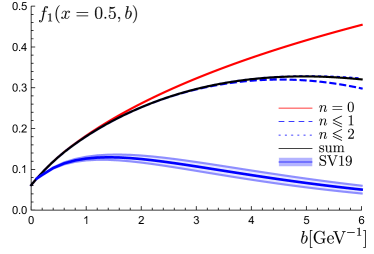
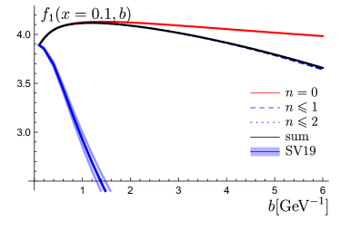
Figure 2: Unpolarized TMD (for d-quark) as the function of $b$ at different orders of mass corrections. The curve $n=0$ corresponds to the leading term. The curves $n\leqslant 1,2$ correspond to the partial sums (83) up to $n=1,2$. In all cases, the PDF is taken in the convolution with NNLO perturbative coefficient function. The curve labeled as “sum” is the summed expression for target-mass corrections (97). The curve with a band is the extraction of non-perturbative TMD distribution $f_{1}$ made in ref.Scimemi:2019cmh .

Sivers $f_{1T}^{\perp}$ and Boer-Mulders $h_{1}^{\perp}$ functions. Sivers and Boer-Mulders functions are given in (4) and (4) correspondingly. Both functions are P-odd, and thus they have a different sign for Drell-Yan and SIDIS configurations Collins:2002kn . In our computation, the sign-flip arises due to the order of integration limits in the irregular terms (79). These are the only terms where the infinite size of the Wilson lines (the parameter $L$) plays a role. The leading power matching for the Sivers function is known for a long time Ji:2006ub ; Kang:2011mr , whereas the leading power matching Boer-Mulders function was derived in Scimemi:2018mmi . Our computation agrees with these references.

In the limit $L\to\mp\infty$ the coefficient function reduces to $\delta(x_{2})$ and thus Sivers and Boer-Mulders functions are expressed through $T(-x,0,x)$ and $\delta T_{\epsilon}(-x,0,x)$ at all powers of $b^{2}$. The function $T(-x,0,x)$ is known as a Qiu-Sterman (QS) function Qiu:1991pp , and $\delta T_{\epsilon}(-x,0,x)$ is the analog of QS function for the chiral-odd operator. Both TMDPDFs are expressed via QS functions at all orders of $b$-expansion. This observation is a non-trivial fact because the QS functions are not autonomous, and mix with the bulk of twist-3 distribution during the evolution Braun:2009mi . The NLO expression for the leading power coefficient function Scimemi:2019gge contains the non-QS but only in the logarithmic terms (i.e., the terms responsible for the evolution effects), whereas the finite part is proportional to the QS function. Based on this information, we make a conjecture that Sivers and Boer-Mulders functions can be expressed entirely through the QS function, up to logarithmic terms.

Helicity $g_{1L}$ and transversity $h_{1}$ TMDs. The helicity and tranversity TMDPDFs are given in (4) and (4) correspondingly. These distributions have leading power matching to the twist-2 distributions. The perturbative coefficients for the leading power matching are known up to NLO Gutierrez-Reyes:2017glx ; Buffing:2017mqm (for helicity) and NNLO Gutierrez-Reyes:2018iod (for transversity). In contrast, to the unpolarized TMD $f_{1}$ (83) distribution $g_{1L}$ and $h_{1}$ have non-zero contribution of twist-3 PDFs. The expressions given in this work do not account the twist-4 PDFs, and thus already the $n=1$ term is incomplete and contains additional twist-4 contribution (see also fig.1).

Worm-gear TMDs $g_{1T}$ and $h_{1L}^{\perp}$. The worm-gear distributions $g_{1T}$ and $h_{1L}^{\perp}$ are given in (4) and (4), correspondingly. They have the generic structure of distributions with the leading power matching at collinear twist-3 operator (see fig.1). Both worm-gear TMDPDFs have the factor $x$, which suppresses them at small-$x$. It is interesting to mention that despite both distribution have similar form, TMD $g_{1T}$ is expected to be much larger according to a recent measurement Airapetian:2020zzo . The leading power expressions for both distributions were derived in Kanazawa:2015ajw (using Lorentz invariance relations) and Scimemi:2018mmi (using the off-light-cone parametrization), and agree with our computation.

Pretzelosity TMD $h_{1T}^{\perp}$. The expression for the pretzelosity TMD is given in (4). The expression (4) demonstrates a non-trivial value for pretzelosity distribution for the first time. The leading power term for the pretzelosity reads

$$h_{1T}^{\perp}(x,b)=-x^{2}\int_{0}^{1}du\int dy\delta(x-uy)\frac{1-u^{2}}{u}\mathcal{T}_{h}(y).$$ (98)

This expression is incomplete, because at the same level of accuracy PDFs of twist-4 could contribute. Thus eqn.(98) is only the Wandzura-Wilchek approximation to the full expression. Note, that unless $\mathcal{T}_{h}(x)$ has some anomalously strong behavior, (that could happen only at $x\to 0$, since $\mathcal{T}_{h}(1)=0$) the pretzelosity distribution is a very small function. At $x\to 1$ the convolution is suppressed by the factor $(1-u^{2})$, whereas at $x\to 0$ there is a common factor $x^{2}$. This observation is in a general agreement with the experimental data Airapetian:2020zzo ; Lefky:2014eia , which is compatible with zero for the pretzelosity-involving observables.

There are no contribution of twist-2 PDFs. The absence of matching to twist-2 PDFs is true for all orders of the perturbation theory that were checked in ref.Gutierrez-Reyes:2018iod up to $\alpha_{s}^{2}$-order, and discussed in ref.Chai:2018mwx . This fact can be proven comparing the following combinations of chiral-odd TMDPDFs

$$b_{\alpha}\Phi^{[i\sigma^{\alpha+}\gamma_{5}]}(x,b) = (bs_{T})\left(h_{1}(x,b)+\frac{M^{2}b^{2}}{2}h_{1T}^{\perp}(x,b)\right)-i\lambda b^{2}Mh_{1L}^{\perp}(x,b),$$ (99)

$$b_{\alpha}\epsilon_{T}^{\alpha\beta}\Phi^{[i\sigma^{\beta+}\gamma_{5}]}(x,b) = (b_{\alpha}\epsilon^{\alpha\beta}s_{\beta})\left(h_{1}(x,b)-\frac{M^{2}b^{2}}{2}h_{1T}^{\perp}(x,b)\right)-ib^{2}Mh_{1}^{\perp}(x,b).$$ (100)

The non-zero pretzelosity appears only if the matrix element $\Phi^{[i\sigma^{\alpha+}\gamma_{5}]}$ has terms with different parity (so the expressions in (99,100) in brackets are different). At the twist-2 level there is only one PDF, and thus the pretzelosity is null. At the twist-3 level there are pairs of operators with different parity: e.g. $\bar{\psi}_{+}f_{++}\bar{\chi}_{+}$ and $\bar{\psi}_{+}\bar{f}_{++}\bar{\chi}_{+}$ which produce asymmetry in (99,100), because $\langle p,S|\bar{\psi}_{+}\bar{f}_{++}\bar{\chi}_{+}|p,S\rangle=0$. Since QCD Lagrangian conserves parity, these statements are generally preserved at any order of perturbative expansion in a properly defined regularization scheme. In the dimension regularization the Levi-Civita tensor is not uniquely defined and thus the symmetry between relations (99,100) could be violated. In this case, one observes the non-zero pretzelosity Gutierrez-Reyes:2017glx ; Gutierrez-Reyes:2018iod in the $\epsilon$-suppressed terms. However, it is only an artifact of the dimensional regularization, and it must vanish at $\epsilon\to 0$. The same statement holds for the quasi-TMDs for which the non-trivial but $\epsilon$-suppressed matching to pretzelocity has been observed in ref.Ebert:2020gxr at $\alpha_{s}$-order.

5 Conclusion

		Twist of	Twist-2	Twist-3	Order of
Name	Function	leading	distributions	distributions	leading power	Ref.
		matching	in matching	in matching	coef.function
unpolarized	$f_{1}(x,b)$	tw-2	$f_{1}(x)$	–	N3LO ($\alpha_{s}^{3}$)	Luo:2019szz ; Ebert:2020yqt
Sivers	$f_{1T}^{\perp}(x,b)$	tw-3	–	$T(-x,0,x)$	NLO ($\alpha_{s}^{1}$)	Scimemi:2019gge
helicity	$g_{1L}(x,b)$	tw-2	$g_{1}(x)$	$\mathcal{T}_{g}(x)$	NLO ($\alpha_{s}^{1}$)	Gutierrez-Reyes:2017glx ; Buffing:2017mqm
worm-gear T	$g_{1T}(x,b)$	tw-2/3	$g_{1}(x)$	$\mathcal{T}_{g}(x)$	LO ($\alpha_{s}^{0}$)	Kanazawa:2015ajw ; Scimemi:2018mmi
transversity	$h_{1}(x,b)$	tw-2	$h_{1}(x)$	$\mathcal{T}_{h}(x)$	NNLO ($\alpha_{s}^{2}$)	Gutierrez-Reyes:2018iod
Boer-Mulders	$h_{1}^{\perp}(x,b)$	tw-3	–	$\delta T_{\epsilon}(-x,0,x)$	LO ($\alpha_{s}^{0}$)	Scimemi:2018mmi
worm-gear L	$h_{1L}^{\perp}(x,b)$	tw-2/3	$h_{1}(x)$	$\mathcal{T}_{h}(x)$	LO ($\alpha_{s}^{0}$)	Kanazawa:2015ajw ; Scimemi:2018mmi
pretzelosity	$h_{1T}^{\perp}$	tw-3/4	–	$\mathcal{T}_{h}(x)$	LO ($\alpha_{s}^{0}$)	eq.(4)

Table 1: Summary of the information on the collinear matching for quark TMDs.

TMD distributions are related to the collinear distributions in the limit of small-$b$. In the present work, we have studied this relation at all powers of $b$-expansion and derived the contributions with twist-2 and twist-3 PDFs. Our computation includes all eight polarized TMDs. From the perspective of the resummation approach, the computed corrections are target-mass corrections. The summary of the here-derived and known results is presented in table 1. It is the first study of the matching between TMDPDF and collinear PDFs beyond the leading power, to our best knowledge. Thus, many results and conclusions made in this paper are novel.

The list of expression for TMDPDFs is presented in sec.4. All expressions have the following common structure

$$F(x,b)=\sum_{n=0}^{\infty}\left(\frac{x^{2}b^{2}M^{2}}{4}\right)^{n}\frac{1}{n!n!}\left[\left(\frac{\bar{u}}{u}\right)^{n}G_{n}(u)\otimes f\right](x),$$ (101)

where $F$ is a TMD distribution, $f$ is a (combination of) collinear distribution, and $\otimes$ is the Mellin convolution. In addition to the power-suppression each term is accompanied by the factor $x^{2n}$. Due to its numerical value of computed correction is almost negligible. The appearance of target-mass corrections in the combination $(x^{2}M^{2})$ justifies the usage of proton TMDPDF for nuclei. For nuclear observables the target-mass is $Z$-times larger, but the measured $x$ is $Z$-times smaller (with $Z$ being the atomic number). Together these factors compensate each other, and thus the nuclear TMDPDF is roughly a nucleon TMDPDF. The knowledge of target-mass corrections is also essential for lattice computations of polarized quasi-TMDPDFs Vladimirov:2020ofp ; Ebert:2020gxr .

One of the central results of this work is the elaboration of the twist-decomposition-method. The method is taken from Braun:2008ia ; Braun:2009mi and uses the simplifications of the spinor formalism. In the present study, it is applied at the tree-order, but similarly it can be used together with loop-calculation. Let us note that the computation is made in the position space, which is the only straightforward way to compute such power corrections. It is clear that each term with $n>0$ of the expansion (101) is power-divergent in the the momentum space. Moreover, the resummed series of power corrections (97) also has a divergent Fourier transform. It demonstrates the well-known fact that at certain $b$, the perturbative series (in any form) fails to describe non-local objects, and truly non-perturbative effects must be accounted.

For the first time, we derive the non-zero matching of pretzelosity distribution to the collinear distributions. Its leading power expression contains twist-3 (given in (98)) and twist-4 PDFs (not computed). Previously there were unsuccessful attempts to find a non-zero matching of pretzelosity to twist-2 PDFs Gutierrez-Reyes:2017glx ; Gutierrez-Reyes:2018iod . In sec.4 we provide the argumentation of why the pretzelosity does not have a contribution of twist-2 PDFs at all orders of power and $\alpha_{s}$ corrections.

Appendix A Twist-3 part of the operators $O_{s,n,t}$

In this appendix, we collect the expressions for twist-3 parts of the operators $O_{s,n,t}$. The definition of operator $\hat{T}_{3}$ is given in (64,65). The definition of the operator $O_{s,n,t}$ is given in (51,66). The route of derivation is explained in sec.3.2.

The twist-3 part of chiral-even operators are

$$\hat{T}_{3}^{(\bar{\mu}\bar{\lambda})}O_{s,n,t}^{\bar{\psi}_{+}\psi_{+}} = 2ig\sum_{k=1}^{n}\left(\frac{\mu\partial}{\partial\lambda}\right)^{n-k}\left(\frac{\bar{\mu}\partial}{\partial\bar{\lambda}}\right)^{k-1}$$

$$\frac{(-1)^{t}(n-1)!}{(k-1)!(n-k)!}\frac{(s+t+n-k)!(s+t+n)}{(s+t+n+1)!}\frac{(s+t+k+1)!}{(s+t+n+1)!}$$

$$b^{k}\bar{b}^{n-k}(\bar{\lambda}\bar{\mu})\Bigg{\{}(s+t+n+1)n\sum_{m=0}^{s-2}+(s+t+n+1)\sum_{m=s-1}^{s+n-2}(s+n-m-1)$$

$$-n\sum_{m=0}^{s+t+n-2}(s+t+n-m-1)\Bigg{\}}\bar{\psi}_{+}\overleftarrow{D}_{\lambda\bar{\lambda}}^{m}f_{++}\overleftarrow{D}_{\lambda\bar{\lambda}}^{s+t+n-m-2}\psi_{+},$$

$$\hat{T}_{3}^{(\mu\lambda)}O_{s,n,t}^{\bar{\psi}_{+}\psi_{+}} = -2ig\sum_{k=1}^{n}\left(\frac{\bar{\mu}\partial}{\partial\bar{\lambda}}\right)^{n-k}\left(\frac{\mu\partial}{\partial\lambda}\right)^{k-1}$$

$$\frac{(-1)^{s+n}(n-1)!}{(k-1)!(n-k)!}\frac{(s+t+n-k)!(s+t+n)}{(s+t+n+1)!}\frac{(s+t+k+1)!}{(s+t+n+1)!}$$

$$\bar{b}^{k}b^{n-k}(\mu\lambda)\Bigg{\{}(s+t+n+1)n\sum_{m=0}^{t-2}+(s+t+n+1)\sum_{m=t-1}^{t+n-2}(t+n-m-1)$$

$$-n\sum_{m=0}^{s+t+n-2}(s+t+n-m-1)\Bigg{\}}\bar{\psi}_{+}\overrightarrow{D}_{\lambda\bar{\lambda}}^{s+t+n-m-2}\bar{f}_{++}\overrightarrow{D}_{\lambda\bar{\lambda}}^{m}\psi_{+},$$

and

$$\hat{T}_{3}^{(\bar{\mu}\bar{\lambda})}O_{s,n,t}^{\chi_{+}\bar{\chi}_{+}} = \hat{T}_{3}^{(\mu\lambda)}O_{s,n,t}^{\bar{\psi}_{+}\psi_{+}}\{\bar{\psi}_{+}\psi_{+}\to\chi_{+}\bar{\chi}_{+},a\leftrightarrow\bar{a}\},$$ (104)

$$\hat{T}_{3}^{(\mu\lambda)}O_{s,n,t}^{\chi_{+}\bar{\chi}_{+}} = \hat{T}_{3}^{(\bar{\mu}\bar{\lambda})}O_{s,n,t}^{\bar{\psi}_{+}\psi_{+}}\{\bar{\psi}_{+}\psi_{+}\to\chi_{+}\bar{\chi}_{+},a\leftrightarrow\bar{a}\},$$ (105)

where $a\leftrightarrow\bar{a}$ indicates that all barred and unbarred variables should be exchanged, namely $\mu$, $\lambda$, $b$ and $f_{++}$. The twist-3 part of chiral-odd operators have the same general form, but different coefficients in the sum

$$\hat{T}_{3}^{(\bar{\mu}\bar{\lambda})}O_{s,n,t}^{\bar{\psi}_{+}\bar{\chi}_{+}} = 2ig\sum_{k=1}^{n}\left(\frac{\mu\partial}{\partial\lambda}\right)^{n-k}\left(\frac{\bar{\mu}\partial}{\partial\bar{\lambda}}\right)^{k-1}$$

$$\frac{(-1)^{t}(n-1)!}{(k-1)!(n-k)!}\frac{(s+t+n-k+1)!(s+t+n+1)}{(s+t+n+2)!}\frac{(s+t+k)!}{(s+t+n)!}$$

$$b^{k}\bar{b}^{n-k}(\bar{\lambda}\bar{\mu})\Bigg{\{}(s+t+n+2)n\sum_{m=0}^{s-2}+(s+t+n+2)\sum_{m=s-1}^{s+n-2}(s+n-m-1)$$

$$-n\sum_{m=0}^{s+t+n-2}(s+t+n-m)\Bigg{\}}\bar{\psi}_{+}\overleftarrow{D}_{\lambda\bar{\lambda}}^{m}f_{++}\overleftarrow{D}_{\lambda\bar{\lambda}}^{s+t+n-m-2}\bar{\chi}_{+},$$

$$\hat{T}_{3}^{(\bar{\mu}\bar{\lambda})}O_{s,n,t}^{\chi_{+}\psi_{+}} = 2ig\sum_{k=1}^{n}\left(\frac{\mu\partial}{\partial\lambda}\right)^{n-k}\left(\frac{\bar{\mu}\partial}{\partial\bar{\lambda}}\right)^{k-1}$$

$$\frac{(-1)^{t}(n-1)!}{(k-1)!(n-k)!}\frac{(s+t+n-k+1)!(s+t+n+1)}{(s+t+n+2)!}\frac{(s+t+k)!}{(s+t+n)!}$$

$$b^{k}\bar{b}^{n-k}(\bar{\lambda}\bar{\mu})\Bigg{\{}(s+t+n)n\sum_{m=0}^{s-2}+(s+t+n)\sum_{m=s-1}^{s+n-2}(s+n-m-1)$$

$$-n\sum_{m=0}^{s+t+n-2}(s+t+n-m-1)\Bigg{\}}\chi_{+}\overleftarrow{D}_{\lambda\bar{\lambda}}^{m}f_{++}\overleftarrow{D}_{\lambda\bar{\lambda}}^{s+t+n-m-2}\psi_{+},$$

and

$$\hat{T}_{3}^{(\mu\lambda)}O_{s,n,t}^{\bar{\psi}_{+}\bar{\chi}_{+}} = -\hat{T}_{3}^{(\bar{\mu}\bar{\lambda})}O_{s,n,t}^{\chi_{+}\psi_{+}}\{\chi_{+}\psi_{+}\to\bar{\psi}_{+}\bar{\chi}_{+},a\leftrightarrow\bar{a}\},$$ (108)

$$\hat{T}_{3}^{(\mu\lambda)}O_{s,n,t}^{\chi_{+}\psi_{+}} = -\hat{T}_{3}^{(\bar{\mu}\bar{\lambda})}O_{s,n,t}^{\bar{\psi}_{+}\bar{\chi}_{+}}\{\bar{\psi}_{+}\bar{\chi}_{+}\to\chi_{+}\psi_{+},a\leftrightarrow\bar{a}\}.$$ (109)

Appendix B Power corrections for fragmentation functions

In the case of TMDFF the matching to the collinear FF is not entirely defined. The reason is the absence of local-operator expansion for FF-type operators. Only indirect methods of twist-decomposition for FF operators are possible, such as differential equations Balitsky:1990ck , Feynman diagram correspondences Kanazawa:2013uia ; Echevarria:2015usa ; Echevarria:2016scs ; Gamberg:2018fwy and Lorentz invariant relations Kanazawa:2015ajw . However, all these methods are ambiguous, and allow an addition boundary contributions. In this appendix we demonstrate the result which appears if we partially ignores these problems. For detailed discussion we refer to Balitsky:1990ck .

The quark TMDFF is defined as Collins:2011zzd

$$\Delta_{ij}(x,b)=\frac{\mathrm{Tr}_{\text{color}}}{2xN_{c}}\int\frac{dz}{2\pi}e^{-izp^{+}/x}$$ (110)

$$\qquad\sum_{X}\langle 0|[\mp\infty n,0]q_{i}(0)|h(p,s)+X\rangle\langle h(p,s)+X|\bar{q}(zn+b)[zn+b,\mp\infty n+b]|0\rangle,$$

where we use $x$ for collinear fraction of momentum instead of traditional $z$ to avoid the clash of notation. The Wilson lines are connected to $-\infty$ for SIDIS-like process, and to $+\infty$ for $e^{+}e^{-}$-annihilation-like processes. For spinless particles there are only two TMDFFs that contribute to the leading term of the factorization theorem. They read

$$\Delta^{[\gamma^{+}]}(x,b)=D_{1}(x,b),\qquad\Delta^{[i\sigma^{\alpha+}\gamma^{5}]}(x,b)=i\epsilon^{\alpha\mu}_{T}b_{\mu}MH_{1}^{\perp}(x,b).$$ (111)

These functions are called unpolarized ($D_{1}$) and Collins ($H_{1}^{\perp}$) functions. In contrast to the TMDPDF operator, the TMDFF operator cannot be presented as a single T-ordered operator. This is the central issue because it prevents application of OPE. The definition of collinear FF of twist-2,

$$d_{1}(x)=$$ (112)

$$x\frac{\mathrm{Tr}_{\text{color}}}{2N_{c}}\int\frac{dz}{2\pi}e^{-izp^{+}/x}\sum_{X}\langle 0|\frac{\gamma^{+}}{2}[-\infty n,0]q_{i}(0)|h(p,s)+X\rangle\langle h(p,s)+X|\bar{q}(zn)[zn,-\infty n]|0\rangle.$$

Note, that collinear FF is defined with relative factor $x^{2}$ in comparison to TMDFF Collins:2011zzd .

In the case of FF-type operators the procedure described in sec.3 should be modified. The reason is the operator in (110) has two parts which could not be joined under a single T-order sign. So, one must distinguish causal (indicated by $(+)$-sign) and anti-causal (indicated by $(-)$-sign) fields which then interact by a cut-propagator. Altogether it is known as Keldysh technique. In Keldysh technique the TMDFF-operator can be written analogously to (40)

$$O_{\text{TMDFF}}^{\Gamma}(z,b)=\bar{q}^{(-)}(zn+b)[zn+b,\mp\infty n+b]^{(-)}\Gamma[\mp\infty n,0]^{(+)}q^{(+)}(0),$$ (113)

where $[a,b]^{(\pm)}$ is a Wilson line made with $A^{(\pm)}$. TMDFF operator can be decomposed into the series (50) with

$$O^{\Gamma}_{FF;s,n,t} = \bar{q}^{(-)}\overleftarrow{D^{(-)}_{+}}^{s}(b\cdot\overleftarrow{D}^{(-)})^{n}\Gamma\overrightarrow{D^{(+)}_{+}}^{t}q^{(+)}.$$ (114)

Next, one can perform the twist-decomposition for this operator in complete analogy to the TMDPDF operator. The final expressions for twist-2 part (67-68) are analogous, with the only replacement $D_{\lambda\bar{\lambda}}^{s+t+n}\to(D^{(-)}_{\lambda\bar{\lambda}})^{s+n}(D^{(+)}_{\lambda\bar{\lambda}})^{t}$. However, the expression for twist-3 part is significantly modified by addition of extra terms with $F_{\mu\nu}^{(+-)}=ig^{-1}[D_{\mu}^{(+)}D_{\nu}^{(-)}]$. These terms cannot be written in a “quasi-partonic” form. It is an unsolved issue.

The next principal difficulty appears when we combine operators to the non-local form. We have not found a way to perform this procedure on the operator level such that the limit $L\to\pm\infty$ can be taken. Alternatively, we can use the analog of (70)

$$\frac{\mathrm{Tr}_{\text{color}}}{N_{c}}\sum_{X}\langle 0|\gamma^{+}\overrightarrow{D}_{+}^{N}q|h(p,s)+X\rangle\langle h(p,s)+X|\bar{q}\overleftarrow{D}_{+}^{M}|0\rangle=4i^{N+M}p_{\lambda\bar{\lambda}}^{N+1}\int dx\frac{d_{1}(x)}{x^{N+M+1}}.$$ (115)

Let us note that this is not a very well defined expression, because it assumes that LHS is dependent on $N+M$ only, which generally does not hold. Nonetheless, operating in this way we receive the all-order expression for unpolarized TMDFF (compare to (70))

$$D_{1}(x,b) = \frac{d_{1}(x)}{x^{2}}+\sum_{n=1}^{\infty}\int_{1}^{\infty}du\int dy\frac{\delta(x-uy)}{n!(n-1)!}\left(\frac{b^{2}M^{2}}{4x^{2}}\right)^{n}\frac{(u-1)^{n-1}}{u}d_{1}(y).$$ (116)

The most notable part here is the “improper” range of the integration over $u$. The ambiguity in the definition of OPE for FF, allows us to add any function that satisfies Laplace equation. For the detailed discussion we refer to sec.3 and 4 of ref.Balitsky:1990ck , where it is shown that for the unpolarized case a convenient addendum is expression (116) with integration range for $u$ extended to $(0,\infty)$. Subtracting this expression we get

$$D_{1}(x,b) = \frac{d_{1}(x)}{x^{2}}-\sum_{n=1}^{\infty}\int_{0}^{1}du\int dy\frac{\delta(x-uy)}{n!(n-1)!}\left(\frac{b^{2}M^{2}}{4x^{2}}\right)^{n}\frac{(u-1)^{n-1}}{u}d_{1}(y).$$ (117)

This expression satisfies the Gribov-Lipatov relation between diagrams of PDF and FF kinematics Gribov:1972rt . This expression can be also derived from equations (3.23), (3.24) and (5.17) of ref.Balitsky:1990ck , in the same fashion as (83) can be derived from Balitsky:1987bk (see explanation in sec.4). In contrast to TMDPDF case, the target-mass corrections for TMDFF are enhanced by $1/x^{2}$ factor. It makes them large for baryon FFs. For meson TMDFFs these corrections remains small due to the small mass of mesons.

References

- (1) J. Collins, Foundations of perturbative QCD, vol. 32. Cambridge University Press, 11, 2013.
- (2) R. Angeles-Martinez et al., Transverse Momentum Dependent (TMD) parton distribution functions: status and prospects, Acta Phys. Polon. B 46 (2015) 2501–2534, [1507.05267].
- (3) I. Scimemi, A short review on recent developments in TMD factorization and implementation, Adv. High Energy Phys. 2019 (2019) 3142510, [1901.08398].
- (4) T. Becher and M. Neubert, Drell-Yan Production at Small , Transverse Parton Distributions and the Collinear Anomaly, Eur. Phys. J. C 71 (2011) 1665, [1007.4005].
- (5) T. Gehrmann, T. Luebbert and L. L. Yang, Calculation of the transverse parton distribution functions at next-to-next-to-leading order, JHEP 06 (2014) 155, [1403.6451].
- (6) J. Collins, L. Gamberg, A. Prokudin, T. Rogers, N. Sato and B. Wang, Relating Transverse Momentum Dependent and Collinear Factorization Theorems in a Generalized Formalism, Phys. Rev. D 94 (2016) 034014, [1605.00671].
- (7) I. Scimemi and A. Vladimirov, Non-perturbative structure of semi-inclusive deep-inelastic and Drell-Yan scattering at small transverse momentum, JHEP 06 (2020) 137, [1912.06532].
- (8) A. Bacchetta, V. Bertone, C. Bissolotti, G. Bozzi, F. Delcarro, F. Piacenza et al., Transverse-momentum-dependent parton distributions up to N3LL from Drell-Yan data, 1912.07550.
- (9) V. Braun and A. Manashov, Operator product expansion in QCD in off-forward kinematics: Separation of kinematic and dynamical contributions, JHEP 01 (2012) 085, [1111.6765].
- (10) D. Boer, P. Mulders and F. Pijlman, Universality of T odd effects in single spin and azimuthal asymmetries, Nucl. Phys. B 667 (2003) 201–241, [hep-ph/0303034].
- (11) X. Ji, J.-W. Qiu, W. Vogelsang and F. Yuan, A Unified picture for single transverse-spin asymmetries in hard processes, Phys. Rev. Lett. 97 (2006) 082002, [hep-ph/0602239].
- (12) Z.-B. Kang, B.-W. Xiao and F. Yuan, QCD Resummation for Single Spin Asymmetries, Phys. Rev. Lett. 107 (2011) 152002, [1106.0266].
- (13) K. Kanazawa, Y. Koike, A. Metz, D. Pitonyak and M. Schlegel, Operator Constraints for Twist-3 Functions and Lorentz Invariance Properties of Twist-3 Observables, Phys. Rev. D 93 (2016) 054024, [1512.07233].
- (14) I. Scimemi and A. Vladimirov, Matching of transverse momentum dependent distributions at twist-3, Eur. Phys. J. C 78 (2018) 802, [1804.08148].
- (15) A. Accardi, A. Bacchetta and M. Schlegel, What can we learn from the breaking of the Wandzura-Wilczek relation?, AIP Conf. Proc. 1155 (2009) 35–41, [0905.3118].
- (16) D. Gutiérrez-Reyes, I. Scimemi and A. A. Vladimirov, Twist-2 matching of transverse momentum dependent distributions, Phys. Lett. B 769 (2017) 84–89, [1702.06558].
- (17) M. G. A. Buffing, M. Diehl and T. Kasemets, Transverse momentum in double parton scattering: factorisation, evolution and matching, JHEP 01 (2018) 044, [1708.03528].
- (18) M. G. Echevarria, I. Scimemi and A. Vladimirov, Unpolarized Transverse Momentum Dependent Parton Distribution and Fragmentation Functions at next-to-next-to-leading order, JHEP 09 (2016) 004, [1604.07869].
- (19) D. Gutierrez-Reyes, I. Scimemi and A. Vladimirov, Transverse momentum dependent transversely polarized distributions at next-to-next-to-leading-order, JHEP 07 (2018) 172, [1805.07243].
- (20) D. Gutierrez-Reyes, S. Leal-Gomez, I. Scimemi and A. Vladimirov, Linearly polarized gluons at next-to-next-to leading order and the Higgs transverse momentum distribution, JHEP 11 (2019) 121, [1907.03780].
- (21) M.-x. Luo, T.-Z. Yang, H. X. Zhu and Y. J. Zhu, Quark Transverse Parton Distribution at the Next-to-Next-to-Next-to-Leading Order, Phys. Rev. Lett. 124 (2020) 092001, [1912.05778].
- (22) M. A. Ebert, B. Mistlberger and G. Vita, Transverse momentum dependent PDFs at N3LO, 2006.05329.
- (23) I. Scimemi, A. Tarasov and A. Vladimirov, Collinear matching for Sivers function at next-to-leading order, JHEP 05 (2019) 125, [1901.04519].
- (24) R. L. Jaffe, Spin, twist and hadron structure in deep inelastic processes, in Ettore Majorana International School of Nucleon Structure: 1st Course: The Spin Structure of the Nucleon, pp. 42–129, 1, 1996. hep-ph/9602236.
- (25) V. Braun, G. Korchemsky and D. Müller, The Uses of conformal symmetry in QCD, Prog. Part. Nucl. Phys. 51 (2003) 311–398, [hep-ph/0306057].
- (26) I. I. Balitsky and V. M. Braun, The Nonlocal operator expansion for inclusive particle production in e+ e- annihilation, Nucl. Phys. B 361 (1991) 93–140.
- (27) K. Kanazawa and Y. Koike, Contribution of twist-3 fragmentation function to single transverse-spin asymmetry in semi-inclusive deep inelastic scattering, Phys. Rev. D 88 (2013) 074022, [1309.1215].
- (28) M. G. Echevarria, I. Scimemi and A. Vladimirov, Transverse momentum dependent fragmentation function at next-to–next-to–leading order, Phys. Rev. D 93 (2016) 011502, [1509.06392].
- (29) L. Gamberg, Z.-B. Kang, D. Pitonyak, M. Schlegel and S. Yoshida, Polarized hyperon production in single-inclusive electron-positron annihilation at next-to-leading order, JHEP 01 (2019) 111, [1810.08645].
- (30) P. Mulders and R. Tangerman, The Complete tree level result up to order 1/Q for polarized deep inelastic leptoproduction, Nucl. Phys. B 461 (1996) 197–237, [hep-ph/9510301].
- (31) V. Braun, A. Manashov and J. Rohrwild, Renormalization of Twist-Four Operators in QCD, Nucl. Phys. B 826 (2010) 235–293, [0908.1684].
- (32) V. Braun, A. Manashov and J. Rohrwild, Baryon Operators of Higher Twist in QCD and Nucleon Distribution Amplitudes, Nucl. Phys. B 807 (2009) 89–137, [0806.2531].
- (33) H. K. Dreiner, H. E. Haber and S. P. Martin, Two-component spinor techniques and Feynman rules for quantum field theory and supersymmetry, Phys. Rept. 494 (2010) 1–196, [0812.1594].
- (34) I. Balitsky and V. M. Braun, Evolution Equations for QCD String Operators, Nucl. Phys. B 311 (1989) 541–584.
- (35) A. Bacchetta, M. Diehl, K. Goeke, A. Metz, P. J. Mulders and M. Schlegel, Semi-inclusive deep inelastic scattering at small transverse momentum, JHEP 02 (2007) 093, [hep-ph/0611265].
- (36) V. Braun, A. Manashov and B. Pirnay, Scale dependence of twist-three contributions to single spin asymmetries, Phys. Rev. D 80 (2009) 114002, [0909.3410].
- (37) M. Sohnius, Introducing Supersymmetry, Phys. Rept. 128 (1985) 39–204.
- (38) D. Boer, L. Gamberg, B. Musch and A. Prokudin, Bessel-Weighted Asymmetries in Semi Inclusive Deep Inelastic Scattering, JHEP 10 (2011) 021, [1107.5294].
- (39) I. Scimemi and A. Vladimirov, Systematic analysis of double-scale evolution, JHEP 08 (2018) 003, [1803.11089].
- (40) B. Geyer, M. Lazar and D. Robaschik, Decomposition of nonlocal light cone operators into harmonic operators of definite twist, Nucl. Phys. B 559 (1999) 339–377, [hep-th/9901090].
- (41) A. V. Belitsky and D. Mueller, Twist- three effects in two photon processes, Nucl. Phys. B 589 (2000) 611–630, [hep-ph/0007031].
- (42) P. Ball, V. M. Braun, Y. Koike and K. Tanaka, Higher twist distribution amplitudes of vector mesons in QCD: Formalism and twist - three distributions, Nucl. Phys. B 529 (1998) 323–382, [hep-ph/9802299].
- (43) A. Vladimirov, Structure of rapidity divergences in multi-parton scattering soft factors, JHEP 04 (2018) 045, [1707.07606].
- (44) J. C. Collins, Leading twist single transverse-spin asymmetries: Drell-Yan and deep inelastic scattering, Phys. Lett. B 536 (2002) 43–48, [hep-ph/0204004].
- (45) A. A. Vladimirov, Self-contained definition of Collins-Soper kernel, 2003.02288.
- (46) J.-w. Qiu and G. F. Sterman, Single transverse spin asymmetries, Phys. Rev. Lett. 67 (1991) 2264–2267.
- (47) I. Scimemi and A. Vladimirov, Power corrections and renormalons in Transverse Momentum Distributions, JHEP 03 (2017) 002, [1609.06047].
- (48) HERMES collaboration, A. Airapetian et al., Azimuthal single- and double-spin asymmetries in semi-inclusive deep-inelastic lepton scattering by transversely polarized protons, 2007.07755.
- (49) C. Lefky and A. Prokudin, Extraction of the distribution function from experimental data, Phys. Rev. D 91 (2015) 034010, [1411.0580].
- (50) X. Chai, K. Chen and J. Ma, A Note on Pretzelosity TMD Parton Distribution, Phys. Lett. B 789 (2019) 360–365, [1808.10560].
- (51) M. A. Ebert, S. T. Schindler, I. W. Stewart and Y. Zhao, One-loop Matching for Spin-Dependent Quasi-TMDs, 2004.14831.
- (52) A. A. Vladimirov and A. Schäfer, Transverse momentum dependent factorization for lattice observables, Phys. Rev. D 101 (2020) 074517, [2002.07527].
- (53) V. Gribov and L. Lipatov, e+ e- pair annihilation and deep inelastic e p scattering in perturbation theory, Sov. J. Nucl. Phys. 15 (1972) 675–684.