General-relativistic spin system

Abstract

The models of spin systems defined on the Euclidean space provide powerful machinery for studying a broad range of condensed matter phenomena. While the nonrelativistic effective description is sufficient for most of the applications, it is interesting to consider special and general relativistic extensions of such models. Here, we introduce a framework that allows us to construct theories of continuous spin variables on a curved spacetime. Our approach takes advantage of the results of the nonlinear field space theory, which shows how to construct compact phase space models, in particular for the spherical phase space of spin. Following the methodology corresponding to a bosonization of spin systems into the spin wave representations, we postulate a representation having the form of the Klein-Gordon field. This representation is equivalent to the semiclassical version of the well-known Holstein-Primakoff transformation. The general-relativistic extension of the spin wave representation is then performed, leading to the general-relativistically motivated modifications of the Ising model coupled to a transversal magnetic field. The advantage of our approach is its off-shell construction, while the popular methods of coupling fermions to general relativity usually depend on the form of Einstein field equations with matter. Furthermore, we show equivalence between the considered spin system and the Dirac-Born-Infeld type scalar field theory with a specific potential, which is also an example of $k$-essence theory. Based on this, the cosmological consequences of the introduced spin field matter content are preliminarily investigated.

I Introduction

The models of spin systems, for instance the Ising model, Heisenberg model, XY model [1], or Hubbard model [2], provide a theoretical description of such phenomena as magnetism (ferromagnetism and antiferromagnetism), superconductivity, and topological phase transitions [3]. While these models are adequate in the context of the ground-based tabletop experiments, where local Euclidean geometry is the precise approximation, their extensions to a general curved spacetime are almost unknown. Due to the weakness of gravity in the short-distance interactions, it is mostly irrelevant in condensed matter physics. In consequence, surprisingly little is known about the condensed matter phenomena in curved spacetime. Although rather no one would ask the question about what would happen with a ferromagnet during cosmic inflation, the lack of the definite answer reflects theoretical deficiencies in the lattice spin models. Analysis of their relativistic extensions may not only bring us to the better fundamental understanding of the interaction between gravity and spins but also provide theoretical foundations for possible future condensed matter experiments on Earth’s orbit. More abstract thought experiments, like the analysis of a superfluid state in the vicinity of a black hole horizon or the measurement of gravitational waves near a merger of black holes propagating through a spin glass, might be pondered in light of our results as well.

In the case of spin models describing the ground-based laboratory experiments, spins are considered to be attached to given space points, i.e. forming a fixed lattice. Consequently, such models explicitly break general covariance by distinguishing a certain reference frame. A useful step towards a frame-independent formulation is the continuous limit of a spin system, in which a field-theoretic description of spins is obtained. The analogous continuous spin system approximations play a powerful role in theoretical condensed matter physics, e.g. in the theory of topological phase transitions [3].

The system in such a case becomes a spin field $\vec{S}({\bf x})$ defined on some spatial hypersurface $\Sigma$. In the standard condensed matter considerations, the spatial manifold is chosen as $\Sigma=\mathbb{R}^{d}$, where its dimension $d$ is 1, 2, or 3. From this perspective, one could naively presume that the desired generalization of a spin system is provided by the relativistic field theory of the vector field $\vec{S}({\bf x})$, with the constraint on its norm (the spin magnitude) $\forall{\bf x}:||\vec{S}({\bf x})||=\sqrt{\vec{S}({\bf x})\!\cdot\!\vec{S}({\bf x})}=:S$. Such a framework, an example of which is the famous nonlinear $\sigma-$model [7, 8], however, does not lead to the correct theory of a spin field.

In our analysis, we identify the notion of a spin at each point of space with its semiclassical description by a vector $\vec{S}$ and initially restrict to the spatial manifold $\Sigma$ given by the three-dimensional Euclidean space. We are going to construct the relativistic extension of such a continuous distribution of spins. A natural, but naive, proposal for a generalization of a spin field on Euclidean space to either the spatial sector of spacetime or the Cauchy hypersurface constructed through the ADM decomposition does not lead to a well-working model. The reason is that the spin field is not a standard classical tensor field.

In quantum physics, the model of spin is a finite-dimensional Hilbert space representation of the ${\rm SU}(2)$ group of symmetries, i.e., rotations, and the $\mathfrak{su}(2)$ algebra of observables (whose generators are spin operators $\hat{S}^{x}$, $\hat{S}^{y}$, and $\hat{S}^{z}$). The $\mathfrak{su}(2)$ algebra is noncommutative, which leads to the uncertainty relations between the three spin operators and does not allow one to measure them simultaneously. One often considers the auxiliary object that is a vector $\vec{S}$ (called the spin vector), whose components are the expectation values of the $\hat{S}^{x}$, $\hat{S}^{y}$, and $\hat{S}^{z}$ operators in a given state. At the (semi)classical level, this vector spans the phase space ${\cal P}_{S}$, which is the two-sphere $\mathbb{S}^{2}$ of radius $S$, equipped with a natural symplectic form (cf. [9, 10]). $\mathbb{S}^{2}$ does not have the structure of a cotangent bundle and, consequently, the decomposition of such a phase space into the product of configurational and momentum subspaces is possible only locally. The distinction between a configuration and a momentum of spin becomes clear in the context of the spin precession in a constant magnetic field, whose Hamiltonian we consider in this paper, since one angle on ${\cal P}_{S}$ can be used to parametrize the circle circumscribed by the precessing spin, and the other will be a (constant) angle between the spin vector and the magnetic field [9]. The interpretation of ${\cal P}_{S}$ as the phase space of spin can also be compared with models of a classical relativistic particle, where, depending on an approach, the phase space of spin in the rest frame is indeed ${\cal P}_{S}$ [11] or is obtained by constraining the product of momentum space (which is given by ${\cal P}_{S}$) and configurational space (which is another $\mathbb{S}^{2}$) [12, 13] or by constraining the product of two unit $\mathbb{S}^{2}$ (i.e., configurations and momenta are described in the same way), with $S$ as a coupling constant [14]. All models that we mention here have their origin in applying the coadjoint orbit method [15] to Poincaré group, and they differ only by a choice of phase space coordinates.

Nevertheless, in this paper, we do not investigate spinning particles but a continuous distribution of spin vectors $\vec{S}=\vec{S}({\bf x})$ (a normalized vector field), which is treated as a system consisting of spherical symplectic manifolds attached at each point of space. Through a procedure of the boson mapping of operator algebras (bosonization), the degrees of freedom associated to a spin distribution can be represented by spin waves (a comprehensive description of this issue is given in [22]). Our particular choice is the classical analog of a spin wave reinterpreted as a bosonic field paired with its conjugate momentum. In this case, we will construct a scalar field representation, with the property that values of the field and its momentum are compactified to the sphere. Such a bosonic representation will allow us to construct the natural extension to a general-relativistic model. Translating it back to the spin vector’s distribution is the main goal of our analysis, defining a method never (up to our knowledge) studied before. Our approach belongs to the recently introduced framework of nonlinear field space theories (NFSTs) [23], which extends the standard field theories to the case where the phase space of a field has the nontrivial topology. This generalization is related to numerous ideas and theories, including principle of finiteness [24], Born reciprocity [25], Relative Locality [26], Metastring Theory [27], and polymer quantization in loop quantum gravity [28]. Some of the relations have been already discussed in detail in Refs. [23, 29, 30, 31]. It is worth noting that, as it has been suggested in the above mentioned literature, the compact phase space versions of NFSTs naturally implement the principle of finiteness of physical quantities, which underlies the Born-Infeld theory. However, the principle in the two theories is implemented in different manners, and a direct relation between the actions of Born-Infeld and NFST has not been found so far. Here, we show that the similarity between these theories is not only conceptual, and a scalar field with the specific relativistic spherical phase space reduces to Dirac-Born-Infeld (DBI)-type scalar field theory [32, 33, 34].

The idea to relate spin systems and scalar fields is enabled by the equal dimensions of the local phase spaces of a spin system ($\mathbb{S}^{2}$) and a scalar field ($\mathbb{R}^{2}$). Based on this observation, a new possibility of linking spin systems with field theories has been proposed in Ref. [29]. The exact matching of phase spaces (of a standard scalar field theory and a spin field model) is obtained by taking the large spin limit ($S\rightarrow\infty$). Following this reasoning, it has been shown that in the large spin limit the continuous Heisenberg XXX model is dual to the nonrelativistic scalar field theory with the quadratic dispersion relation [29]. The result has been thereafter generalized to the Heisenberg XXZ model with a dimensionless anisotropy parameter $\Delta$. In this case, it has been demonstrated that taking both the large spin limit ($S\rightarrow\infty$) and the isotropic limit $\Delta\rightarrow 0$, we reduce the XXZ model to the relativistic Klein-Gordon field [30]. However, if the spin limit is not taken exactly, the next to the leading order terms violate relativistic symmetries [30]. Therefore, the question is whether the construction can be improved to preserve the special relativistic and, furthermore, general relativistic symmetries, and also for the spherical phase space field theories with an arbitrary value of the spin vector norm $S$. The purpose of this paper is to address this issue, directly constructing and analyzing the spin field theory that obeys general relativistic symmetries. What we do differently in the current paper is the relation between a spin field and a scalar field, which is now imposed in way equivalent – at the level of excitations – to the bosonization into spin waves.

The construction of the field formulation is based on the bosonization procedure of the fermionic interactions in a solid spin system. This procedure, first introduced in [40], aims to effectively describe the particle-hole-like excitations in the low-energetic regime [41]. The known phenomenological realization of this method is the Tomonaga-Luttinger liquid model [40, 42], in which, under particular constraints, second-order interactions between electrons are represented by bosonic interactions. The model allows one to derive the exact spectrum of the Hamiltonian operator, free energy of noninteracting fermions, and dielectric constant [41].

The basic excitations of coupled spin systems with fixed, homogeneous distribution of spin vectors (but not their orientations) are called spin waves (see [22] for a detailed introduction). One can distinguish two different kinds of such excitations. The first is described by the wave of deflected dipolar magnetic moments produced by elementary spins shifted from their equilibrium positions that propagates through the solid system. This type of excitations is significant at very long wavelengths, comparable to the spacing between individuals, and forms a macroscopic characteristic of the system. The second type of excitations relates to microscopic (quantum) properties of the spin lattice and is relevant for very short wavelengths, comparable with the lattice spacing. In both cases, in the simplest realization, only the nearest-neighbor interactions are considered, forming a net of oscillators.

Since we are interested in the continuous limit, in which the lattice spacing tends to zero, the first type of excitations is relevant in our context. Furthermore, we are interested in the semiclassical description of the spin waves, understood as the linearly propagating vector’s precession phase. When one considers closely spaced frequency components, they can be viewed as a wave packet that moves like a particle. This quasiparticle is called a magnon, and it does not obey the Pauli exclusion principle. We are going to describe properties of this bosonic field in the semiclassical picture, in which the spin variables are represented by the field variables corresponding to the matrix elements of the bosonic operators. The latter ones are constructed in the (semi)classical equivalent of the Holstein-Primakoff transformation [16] (see Appendix A for details), which is one of the most popular maps selected for the bosonization procedure.

The paper is organized as follows. In Sec. II, a spin-related spherical phase space and its scalar field-type parametrization are introduced. Then, in Sec. III, a general strategy behind the defining of the Hamiltonian of the spin system is discussed, based on which, in Sec. IV, the special relativistic spin system is introduced. The results are generalised to the curved spacetime case in Sec. V. In Sec. VI, the obtained model is shown to be be an example of the DBI-type $k$-essence model. Due to the cosmological relevance of the $k$-essence models, consequences of the considered field theory in the dynamics of Universe are preliminarily investigated in Sec. VII. The results are summarized and additional discussion is given in Sec. VIII.

II Phase space of a spin

As we mentioned in the Introduction, we will mostly restrict to the semiclassical description of spin by the vector $\vec{S}=(S^{x},S^{y},S^{z})$, whose components are the generators of proper rotations in the three-dimensional Euclidean space (in other words, it is an element of the Lie algebra of rotations). Although the corresponding classical symmetry group is ${\rm SO}(3)$, we are more interested in another group, ${\rm SU}(2)$. The latter one is a double cover of the former; two-spheres are orbits of both of them, and their Lie algebras are isomorphic. The double cover property, which leads to the appearance of half-integer spins in the quantum theory, is the reason for selecting it to construct models of spin, as we do in this paper.

Another interesting property of spin is its dimension, $[ML^{2}T^{-1}]$. It is the dimension of the classical angular momentum or the Planck constant, $\hbar$. It is worth noting that this is also the dimension of the physical action. The latter property already suggests that the geometrical interpretation of spin is linked with the phase space. In general, states of a classical spin (i.e., the intrinsic angular momentum assumed to be the classical counterpart of spin) are different directions in $\mathbb{R}^{3}$, equivalent to points on $\mathbb{S}^{2}$, and therefore, elements of such a space of states are naturally represented by two angles, $(\phi,\theta)$. As long as we do not define the associated conjugate momenta as belonging to some extra space (as in certain models of spinning particles mentioned in the Introduction), $\mathbb{S}^{2}$ spanned by $\vec{S}$ should actually be interpreted as the phase space of spin. The latter claim can be justified by applying the Kirillov orbit method [15] to the group ${\rm SO}(3)$ (see [10]) or ${\rm SU}(2)$. The method allows one to construct a given phase space as a coadjoint orbit of a symmetry group $G$ (i.e. an orbit in $\mathfrak{g}^{*}$, e.g. $\mathfrak{su}(2)^{*}\cong\mathbb{R}^{3}$) for which the considered mechanical system remains invariant, while the corresponding quantum system should be described by an irreducible unitary representation of $G$. It is well known that two-spheres are coadjoint orbits of $G={\rm SU}(2)$, as evidenced by the fact that a coset ${\rm SU}(2)/{\rm U}(1)\cong\mathbb{S}^{2}$ is the unit two-sphere. In consequence, the quantum models of spin are given by irreducible unitary representations of the ${\rm SU}(2)$ group, labeled by half-integers $s=\frac{n}{2}$, where $n\in\mathbb{N}\cup\{0\}$, as expected.

In order to treat $\mathbb{S}^{2}$ as the phase space of the spin, one has to equip it with a symplectic form (a closed two-form) so that it becomes a symplectic manifold. The natural choice for such a form is the area form, $\omega=S\sin\theta d\phi\wedge d\theta$, where $(\phi,\theta)$ are the usual spherical coordinates. This allows us to introduce a Poisson bracket via the standard definition (turning $\mathbb{S}^{2}$ into a Poisson manifold),

$$\left\{f,g\right\}:=(\omega^{-1})^{ij}(\partial_{i}f)(\partial_{j}g)\,.$$ (1)

Here, $f$ and $g$ are some smooth functions on phase space and $\omega^{-1}$ is inverse of the symplectic form $\omega$. Every Poisson bracket is a Lie bracket by definition. Calculating Eq. (1) for components of the spin vector $\vec{S}$, we verify that they generate the $\mathfrak{su}(2)$ Lie algebra $\left\{S_{i},S_{j}\right\}=\epsilon_{ijk}\!\>S^{k}$. Furthermore, integrating the symplectic form over the whole solid angle, we find that the area of phase space is

$$\int_{\!4\pi}\!\!\omega=4\pi S<\infty\,,$$ (2)

which correctly has the dimension of the Planck constant. If we subsequently follow the topological quantization procedure, the finiteness of the phase space area leads to a specific, discrete spectrum of each of the three operators $\hat{S}_{i}$, as well as the spin square operator $\hat{\vec{S}}^{2}$.

Let us now construct a continuous system of spins, whose phase space at each point of (physical) space is a two-sphere. Components of a continuous spin variable, $\vec{S}({\bf x})=(S^{x}({\bf x}),S^{y}({\bf x}),S^{z}({\bf x}))$, are functions of a position vector ${\bf x}$ and satisfy the $\mathfrak{su}(2)$ algebra bracket in the distributional sense,

$$\left\{S^{i}({\bf x}),S^{j}({\bf y})\right\}=\epsilon^{ijk}\!\>S_{k}({\bf x})\,\delta^{(3)}({\bf x-y})\,,$$ (3)

where $i,j,k\in\left\{x,y,z\right\}$ are the internal indices. Since the Poisson algebra, spanned by spin components, is three-dimensional, it is associated with one propagating degree of freedom and one Casimir invariant, $\vec{S}^{2}\!:=\vec{S}\!\cdot\!\vec{S}\in{\rm const}$. To simplify the formalism, we may characterize the spin system by a parameter $S$ (spin magnitude), assumed to be a constant in space and defined as

$$S:=||\vec{S}||=\sqrt{\vec{S}\cdot\vec{S}}\,.$$ (4)

In the limit where $S$ is very large compared with all other scales, we will require that the ordinary scalar field theory is recovered [cf., (13)]. Let us also emphasize that the spin magnitude is a scalar with respect to symmetry transformations [cf., the constraint (9) that we impose below] and that it appears in the map [Eqs. (5)–(7)] as a scaling factor. Thus, the value of $S$ for a given system is fixed up to a choice of units, i.e., its relation to other constants appearing in our further construction. This relation will be determined by the requirements that the Poisson algebra remains $\mathfrak{su}(2)$ and that the model of a spin system matches the Klein-Gordon field theory [see Eq. (9) and Eqs. (14)–(16)].

In principle, $S$ could become a dynamical quantity in a quite natural generalization of the discussed theory. For example, one might consider the quantization of $S^{2}$. The corresponding operator has a nontrivial spectrum, and its expectation value is determined by the characteristics of a quantum state, which is dynamical. However, in the present classical case, as noted above, $S$ is a Casimir of (the universal enveloping algebra of) the Poisson algebra and hence is fixed at all times by construction.

At the next step, we set the correspondence between the phase spaces of a spin system and a scalar field. We choose to do it by introducing the canonical parametrization of the sphere (at every point ${\bf x}$) in the following way:

$$S^{x} :=S\sqrt{1-\frac{\pi^{2}_{\varphi}}{R^{2}_{\pi}}}\,\cos\left(\frac{\varphi}{R_{\varphi}}\right),$$ (5)

$$S^{y} :=S\sqrt{1-\frac{\pi^{2}_{\varphi}}{R^{2}_{\pi}}}\,\sin\left(\frac{\varphi}{R_{\varphi}}\right),$$ (6)

$$S^{z} :=S\frac{\pi_{\varphi}}{R_{\pi}}\,,$$ (7)

where $\pi_{\varphi}\in[-R_{\pi},R_{\pi}]$ and $\varphi\in(-\pi R_{\varphi},\pi R_{\varphi}]$. The latter coordinates are related to spherical ones $\theta,\phi$ via $\frac{\pi_{\varphi}}{R_{\pi}}=\cos\theta$, $\frac{\varphi}{R_{\varphi}}=\phi$ (up to trivial shifts of the ranges of angles). The fields $\varphi({\bf x})$ and $\pi_{\varphi}({\bf x})$ are then linearlike canonical variables [cf. (11)], in terms of which, we will be able to recover the ordinary scalar field, after choosing the appropriate Hamiltonian.

Similar to spherical coordinates, $\varphi,\pi_{\varphi}$ obviously do not cover the whole sphere; i.e., $\varphi$ is ambiguously defined at the poles $\pi_{\varphi}=\pm R_{\pi}$. In order to extend the map [Eqs. (5)–(7)] everywhere, one has to make an analytic continuation. On the other hand, for the Hamiltonian [Eq. (III)] that we will consider in this paper, the only phase space trajectories that approach the poles are the ones going along two pieces of the meridian $\varphi=\pm\sqrt{\frac{S}{m}}\frac{\pi}{2}$, where Eq. (III) vanishes (see Fig. 2). Thus, these two trajectories can be consistently joined into a single one. The Hamiltonian Eq. (III) is globally defined on $\mathbb{S}^{2}$ in terms of coordinates $S^{x},S^{y},S^{z}$ as Eq. (12), and the latter actually vanishes at the poles as well. Furthermore, the restricted range of applicability of $\varphi,\pi_{\varphi}$ does not pose a problem from the perspective of the considered spin-field correspondence, which is valid only in the regime of small field values – or equivalently large spin magnitude – far away from the poles (see the next section; in particular, Figs. 1 and 2).

The constants $R_{\varphi}$ and $R_{\pi}$ were introduced due to dimensional reasons. They play roles of parameters, which control the accuracy in recovering the standard form of the scalar field’s Hamiltonian in the large $S$ limit. Moreover, as mentioned earlier, we expect only one independent Casimir invariant because the rank of the $\mathfrak{su}(2)$ algebra is two, and its dimension is three. Therefore, performing a canonical rescaling, one can eliminate $R_{\pi}$ and $R_{\varphi}$ in favor of $S$. It is worth noting that when we consider the general-relativistic perspective, the weights of the scalar $\varphi$ and the scalar density $\pi_{\varphi}$ will become relevant. Consequently, the parameters $R_{\pi}$ and $R_{\varphi}$ would also become a scalar and a scalar density, respectively.

In order to determine how the constants $R_{\varphi}$ and $R_{\pi}$ depend on $S$, we use the canonical bracket in the field formulation. The Poisson bracket is defined as usual,

$$\{A,B\}_{\varphi,\pi}:=\int\!d^{3}z\left(\frac{\delta A}{\delta\varphi({\bf z})}\frac{\delta B}{\delta\pi({\bf z})}-\frac{\delta A}{\delta\pi({\bf z})}\frac{\delta B}{\delta\varphi({\bf z})}\right),$$ (8)

where $A:=A[\varphi({\bf x}),\pi_{\varphi}({\bf x})]$ and $B:=B[\varphi({\bf y}),\pi_{\varphi}({\bf y})]$ are arbitrary functionals. Computing the following relation, $\left\{S^{z},S^{x}\right\}_{\varphi,\pi}=\frac{S}{R_{\varphi}R_{\pi}}S^{y}$, it is easy to see that to maintain consistency with the $\mathfrak{su}(2)$ algebra, the parameters have to be related via a simple equation

$$R_{\varphi}R_{\pi}=\sqrt{q}\,S\,.$$ (9)

This relation provides a constraint between the parameters $R_{\varphi}$, $R_{\pi}$ and the Casimir invariant $S$. In Eq. (15), we will choose a specific solution to this constraint such that our model matches the Klein-Gordon Hamiltonian in the low-energy limit. Since $R_{\varphi}$, $R_{\pi}/\sqrt{q}$ and $S$ have trivial Poisson brackets in this system, Eq. (9) does not generate a flow that could leave the constraint surface.

Notice that we introduced above the quantity $q$, denoting the determinant of the spatial metric tensor $q_{ab}$ (which encodes invariance under spatial diffeomorphisms in the field formulation of the model) on the Cauchy hypersurface — from the general-relativistic perspective, this would balance both sides of the identity. It would also modify the Levi-Civita symbol in Eq. (3), which would no longer be a tensor, but a totally antisymmetric tensor codensity (of weight $-1$),

$$\epsilon_{abc}:=\frac{1}{\sqrt{q}}\tilde{\epsilon}_{abc}\,.$$ (10)

Here, $\tilde{\epsilon}_{abc}$ is a tensor, while the indices $a,b,c,...$, which replaced $i,j,k,...$, emphasize that the considered space may be curved. The former set of indices labels the internal coordinates (in the spin formulation) curved accordingly to the spatial coordinates (in the field formulation) due to the dependence on the same metric, $q_{ab}$.

Provided the identity in Eq. (9) is satisfied, the algebra in Eq. (3) is consistent with the assumption that the pair $\varphi$ and $\pi_{\varphi}$ satisfy the standard canonical bracket,

$$\left\{\varphi({\bf x}),\pi_{\varphi}({\bf y})\right\}_{\varphi,\pi}=\delta^{(3)}({\bf x}-{\bf y})\,.$$ (11)

Let us also mention that we are interested in the cosmological application of the discussed spin-field correspondence. The standard form of the Poisson bracket will simplify the description of the cosmological perturbations, allowing one to perform a decomposition of the phase space into homogeneous and inhomogeneous parts in the standard way [43].

It is necessary to stress that the parametrization [Eqs. (5)–(7)] has been chosen so that the $\varphi$ and $\pi_{\varphi}$ fields satisfy the canonical bracket Eq. (11). This is different from the spherical parametrization considered in Refs. [29, 30, 44], which led to a modified form of the canonical relation between the field variables $\varphi$ and $\pi_{\varphi}$.

The canonical parametrization of $\mathfrak{su}(2)$ [Eqs. (5)–(7)] is technically advantageous due to the harmonic behavior of the variables in the vicinity of the classical minimum and the canonical relationship between the scalar field $\varphi$ and its momentum. On the other hand, its form might appear contrived. In order to motivate the form of this parametrization we note that it is the semiclassical limit of the well-known Holstein-Primakoff transformation [16, 45]. This transformation expresses $\mathfrak{su}(2)$ generators in terms of creation and annihilation operators, furnishing the crucial canonical structure. While it is not difficult to demonstrate the correspondence between the Holstein-Primakoff transformation and our canonical parametrization, the details of this semiclassical limit are too long to be included here and, therefore, were moved to Appendix A.

III Spin-field correspondence

Let us consider the following Hamiltonian

$$H:=-\gamma\int d^{3}xS^{x}\,,$$ (12)

where $\gamma$ is a certain constant. In condensed matter physics, it would be interpreted as the interaction term of a continuous distribution of internal magnetic moments (spins) with an external homogeneous magnetic field oriented along the $x$ axis. In the absence of other interactions, a spin at each point would precess around the ground state, $\vec{S}=(S,0,0)$. Meanwhile, the same system, described in terms of the $\varphi$ and $\pi_{\varphi}$ variables, would correspond to a set of oscillators, which become harmonic when the precession angle tends to zero, which is pictorially represented in Fig. 1.

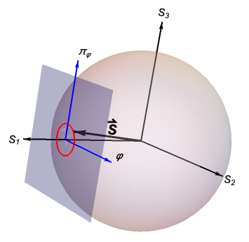
Figure 1: Illustration of the precession of a spin vector $\vec{S}$ around the ground state $\vec{S}=(S,0,0)$, which corresponds to $(\varphi,\pi_{\varphi})=(0,0)$. For the precession angle tending to zero, the dynamics is approximately described by harmonic oscillations at the $(\varphi,\pi_{\varphi})$ phase space. In general, our parametrization maps a hemisphere into a nonsquare rectangle (cf., Fig. 2).

To make the spin-field correspondence evident, let us substitute the expression for $S^{x}$ given by (5) into the Hamiltonian in Eq. (12), finding,

$$H =-\gamma S\int d^{3}x\sqrt{1-\frac{\pi^{2}_{\varphi}}{R^{2}_{\pi}}}\,\cos\left(\frac{\varphi}{R_{\varphi}}\right)$$

$$=\int d^{3}x\left[-\gamma S+\left(\frac{\gamma S}{R^{2}_{\pi}}\right)\frac{\pi^{2}_{\varphi}}{2}+\left(\frac{\gamma S}{R^{2}_{\varphi}}\right)\frac{\varphi^{2}}{2}\right]$$

$$+\mathcal{O}(\pi^{4}_{\varphi},\pi^{2}_{\varphi}\varphi^{2},\varphi^{4})\,.$$ (13)

Up to the constant factor $-\gamma S$, the leading order terms describe the free homogeneous scalar field. From the mechanical perspective, the field is simply a continuous distribution of harmonic oscillators. Furthermore, the form of the Hamiltonian in Eq. (12) has been chosen in the way supporting the correspondence between its ground state $\vec{S}=(S,0,0)$ and the field configuration $(\varphi,\pi_{\varphi})=(0,0)$.

The standard Klein-Gordon form of the Hamiltonian requires the following setting of parameters, $\frac{q\gamma S}{R^{2}_{\pi}}=1$ and $\frac{\gamma S}{R^{2}_{\varphi}}=m^{2}$, where $m$ is the self-interaction constant – the mass of $\varphi$, while $q$ balances the weights on both sides of the former identity. These two relations combined with the one in Eq. (9) are equivalent to the set of three equations:

$$\gamma =m\,,$$ (14)

$$R_{\varphi} =\sqrt{\frac{S}{m}}\,,$$ (15)

$$R_{\pi} =\sqrt{qmS}\,.$$ (16)

The specification of parameters is in general not unique. This one, however, entails the homogeneous Klein-Gordon formulation of the spin wave representation related to the Holstein-Primakoff transformation of the Hamiltonian in Eq. (12), which describes interactions in a continuous distribution of spins in the presence of an external homogeneous magnetic field oriented along the $x$ axis. Let us emphasize that once the transformation in Eqs. (5)–(7), associated with the parametrization (14)–(16), is assumed, it fixes the meaning of the bosonic field’s representation of the spin system. Consequently, it would also specify the quantum spin waves’ kinematics and dynamics, whose solutions on the non-degenerate eigenstates of observables correspond to the excitations of a magnon quasiparticle. This allows one to study bosonic representations of spin systems, which are usually simpler generalizable and coupleable with other fields. Results of any analogous modification in the field formulation of a model are traceable then in the spin formulation.

The parametrization (14)–(16) applied to expression Eq. (13) leads to the following form of the Hamiltonian:

$$H =-mS\int\!d^{3}x\ \sqrt{1-\frac{\pi^{2}_{\varphi}}{Sm}}\,\cos\left(\varphi\sqrt{\frac{m}{S}}\right)$$

$$=-mS\int\!d^{3}x+\int\!d^{3}x\left(\frac{\pi^{2}_{\varphi}}{2}+m^{2}\frac{\varphi^{2}}{2}\right)$$

$$+\mathcal{O}(\pi^{4}_{\varphi},\pi^{2}_{\varphi}\varphi^{2},\varphi^{4})\,,$$ (17)

where we imposed the flat space constraint, $q_{ab}=\delta_{ab}$, simplifying the determinant of the metric tensor to $q=1$. Notice that the first term in the second line diverges with the spacetime volume. This term, however, does not contribute to classical dynamics and, for convenience, can be regulated by performing an infinite subtraction (setting the vacuum energy to zero).

The evolution equations are calculated from the Hamiltonian Eq. (III) in the usual way, via $\dot{\pi}_{\varphi}=\{\varphi,H\}_{\varphi,\pi}$ and $\dot{\varphi}=\{\pi_{\varphi},H\}_{\varphi,\pi}$,

$$\dot{\pi}_{\varphi} =-m\sqrt{mS-\pi_{\varphi}^{2}}\,\sin\left(\varphi\sqrt{\frac{m}{S}}\right)\,,$$

$$\dot{\varphi} =\frac{\sqrt{mS}\,\pi_{\varphi}}{\sqrt{mS-\pi_{\varphi}^{2}}}\cos\left(\varphi\sqrt{\frac{m}{S}}\right)\,.$$ (18)

Clearly, in the limit $S\rightarrow\infty$, the standard relations $\dot{\varphi}=\pi_{\varphi}$ and $\dot{\pi}_{\varphi}=-m^{2}\varphi$ are correctly recovered. The solutions of the above equations for $\varphi\in\left(-\frac{\pi}{2}\sqrt{\frac{S}{m}},\frac{\pi}{2}\sqrt{\frac{S}{m}}\right)$ can be written as (cf., [31]),

$$\pi_{\varphi}(t) =-C\sqrt{mS}\,\sin(m(t-t_{0}))\,,$$

$$\varphi(t) =\sqrt{\frac{S}{m}}\,\arcsin\left(\frac{C\cos(m(t-t_{0}))}{\sqrt{1-C^{2}\sin^{2}(m(t-t_{0}))}}\right)\,.$$ (19)

If we assume the initial condition for $\pi_{\varphi}$, $\pi_{\varphi}(t_{0})=0$, a constant $C=\sin(\sqrt{\frac{m}{S}}\,\varphi_{0})$ encodes the other initial condition $\varphi(t_{0})=\varphi_{0}\in\left[0,\frac{\pi}{2}\sqrt{\frac{S}{m}}\right)$, equivalent to $\varphi(t_{0}+\frac{\pi}{m})=-\varphi_{0}\in\left(-\frac{\pi}{2}\sqrt{\frac{S}{m}},0\right]$. The reason that we can restrict to setting an initial condition for $\varphi$ in the range $\left[0,\frac{\pi}{2}\sqrt{\frac{S}{m}}\right)$ is that all phase space trajectories $(\pi_{\varphi},\varphi)$ are closed curves, as depicted in Fig. 2. Moreover, in the limit $\varphi_{0}\to\frac{\pi}{2}\sqrt{\frac{S}{m}}$, we have $\varphi(t)=\pm\varphi_{0}|_{-\sqrt{mS}<\pi_{\varphi}<\sqrt{mS}}$. These are the only trajectories that reach the ill-defined boundaries $\pi_{\varphi}=\pm\sqrt{mS}$ (corresponding to poles of the sphere), and hence, their ending points can be pairwise identified in the unambiguous way. The formulae in Eq. (III) can be also analytically continued to the other hemisphere, leading to the mirror image.

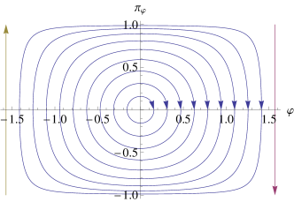
Figure 2: A sample of phase space trajectories Eq. (III) on the hemisphere with $\varphi\in\left[-\frac{\pi}{2}\sqrt{\frac{S}{m}},\frac{\pi}{2}\sqrt{\frac{S}{m}}\right]$, for $S=1$, $m=1$; the arrows denote the direction of time.

The first equation in Eq. (III) can be rewritten in the form:

$$\frac{\sqrt{1-\frac{\pi^{2}_{\varphi}}{mS}}}{\sqrt{mS}\cos\left(\varphi\sqrt{\frac{m}{S}}\right)}=\pm\frac{1}{\sqrt{\dot{\varphi}^{2}+mS\cos^{2}\left(\varphi\sqrt{\frac{m}{S}}\right)}}\,.$$ (20)

The $\pm$ sign corresponds to $\varphi\in{\cal F}_{+}$ or $\varphi\in{\cal F}_{-}$, respectively, where these two sectors of possible values of $\varphi$ (associated with two hemispheres) are

$${\cal F}_{+}:=\sqrt{\frac{S}{m}}\,\left(-\frac{\pi}{2},\frac{\pi}{2}\right)\,,$$ (21)

$${\cal F}_{-}:=\sqrt{\frac{S}{m}}\,\left(\left(-\pi,-\frac{\pi}{2}\right)\cup\left(\frac{\pi}{2},\pi\right]\right)\,,$$ (22)

while for $\varphi=\pm\sqrt{\frac{S}{m}}\frac{\pi}{2}$, we have $\dot{\varphi}=0$. The sign ambiguity in Eq. (20) has consequences when one performs the inverse Legendre transform to recover the Lagrangian. Namely, we have to define two variants of the Lagrangian,

$$L^{\pm} :=\int\!d^{3}x\ \dot{\varphi}\pi_{\varphi}-H\ |_{\varphi\in{\cal F}_{\pm}}$$

$$=\pm\sqrt{mS}\int\!d^{3}x\ \sqrt{\dot{\varphi}^{2}+mS\cos^{2}\left(\varphi\sqrt{\frac{m}{S}}\right)}$$ (23)

and it vanishes at the meridian $\varphi=\pm\sqrt{\frac{S}{m}}\frac{\pi}{2}$.

The two possible choices for the Lagrangian define dynamics related to two hemispheres of the spherical phase space. However, only $L^{+}$ allows us to recover the standard scalar field theory, corresponding to the large spin limit. This argument specifies the range of the possible values that the considered scalar field can take, $\varphi\sqrt{\frac{m}{S}}\in(-\pi/2,\pi/2)$, and it makes the $\varphi\rightarrow 0$ limit achievable. Consequently, in the expansion of $L^{+}$ around the small field’s values and the related velocities,

$$L^{+} =mS\int\!d^{3}x+\int\!d^{3}x\ \left(\frac{1}{2}\dot{\varphi}^{2}-\frac{1}{2}m^{2}\varphi^{2}\right)$$

$$+\mathcal{O}(\dot{\varphi}^{4},\dot{\varphi}^{2}\varphi^{2},\varphi^{4})\,,$$ (24)

the standard form of the homogeneous scalar field’s Lagrangian is recovered.

IV Special relativistic extension

In the previous section the spin-field correspondence was introduced, where the field side of this relation was constructed in the Hamiltonian formalism. The spin phase space was parametrized in the way leading to the spatially homogeneous Klein-Gordon-like form of the Hamiltonian in the large spin limit. It is, however, much easier to construct an invariant theory at the level of an action – one just has to make sure that the action is a scalar. Difficulties appear when the Poisson bracket associated with a continuous system of spins is non canonical, and therefore derivation of the Lagrangian is neither straightforward, nor trivial. Another argument to focus on the field formalism is the well-known model of the Lorentz-invariant Klein-Gordon field, which is the standard formulation of this theory.

Before we begin generalizing the field side of our framework, let us mention how one could proceed with the spin-side. The standard (special) relativistic generalization of spin is introduced as follows (see, e.g., [46]). A given system has the angular momentum tensor $J^{\mu\nu}=L^{\mu\nu}+S^{\mu\nu}$, where $L^{\mu\nu}=X^{\mu}P^{\nu}-X^{\nu}P^{\mu}$ is the orbital angular momentum, while the intrinsic part (i.e., spin) $S^{\mu\nu}$ can be expressed as $S^{\mu\nu}=\varepsilon^{\mu\nu\alpha\beta}u_{\alpha}S_{\beta}$. Consequently, the spin four-vector (known as Pauli-Lubański vector) is orthogonal to the four-velocity, $u_{\alpha}S^{\alpha}=0$, and in the rest frame, it is simply $(S^{\mu})=(0,\vec{S})$. $M^{\mu\nu}$ and $S^{\mu\nu}$ become mixed under the action of Lorentz transformations unless $M^{\mu\nu}=0$, as in our case. However, what we do in the current paper is quite different. We do not consider the relativistic generalization of a single spin but of a spin field, which is first represented by a scalar field and only then generalized.

Looking for the Lorentz-invariant analog of the correspondence defined by the transformation and parametrization in Eqs. (5)–(7) and Eqs. (14)–(16), respectively, is the primary problem of this section. We are going to achieve our goal by modifying the Lagrangian obtained in Eq. (III). This object is a functional of Lorentz scalars, and in the large spin limit, it takes the form of the homogeneous scalar field Lagrangian. Its generalization is then straightforward,

$$\dot{\varphi}^{2}\rightarrow-\eta^{\mu\nu}\partial_{\mu}\varphi\partial_{\nu}\varphi\,,$$ (25)

where the Minkowski metric, $\eta^{\mu\nu}=\text{diag}(-1,1,1,1)$, was introduced. In consequence, Eq. (III) leads to

$$L^{\pm} =\pm\sqrt{mS}\int\!d^{3}x\ \sqrt{-\eta^{\mu\nu}\partial_{\mu}\varphi\partial_{\nu}\varphi+mS\cos^{2}\left(\varphi\sqrt{\frac{m}{S}}\right)}$$

$$=\pm mS\int\!d^{3}x\pm\int\!d^{3}x\ \left(-\frac{1}{2}\eta^{\mu\nu}\partial_{\mu}\varphi\partial_{\nu}\varphi-\frac{1}{2}m^{2}\varphi^{2}\right)$$

$$+\text{h.o.t.}$$ (26)

(from now on, the abbreviation h.o.t.​ denotes higher order terms). For the $+$ case, the leading order of the Lagrangian describes the standard Klein-Gordon scalar field. The momentum canonically conjugate to $\varphi$ is given by the formula,

$$\pi_{\varphi}:=\frac{\delta L^{\pm}}{\delta\dot{\varphi}}=\pm\frac{\sqrt{mS}\,\dot{\varphi}}{\sqrt{-\eta^{\mu\nu}\partial_{\mu}\varphi\partial_{\nu}\varphi+mS\cos^{2}\left(\varphi\sqrt{\frac{m}{S}}\right)}}\,.$$ (27)

Performing the inverse Legendre transformation, we obtain the Hamiltonian,

$$H^{\pm} =\mp\sqrt{mS}\int\!d^{3}x\ \sqrt{1-\frac{\pi^{2}_{\varphi}}{mS}}\,\sqrt{-(\nabla\varphi)^{2}+mS\cos^{2}\left(\varphi\sqrt{\frac{m}{S}}\right)}$$

$$=\mp mS\int\!d^{3}x\pm\int\!d^{3}x\ \left(\frac{\pi^{2}_{\varphi}}{2}+\frac{1}{2}(\nabla\varphi)^{2}+m^{2}\frac{\varphi^{2}}{2}\right)+\text{h.o.t.}\,,$$ (28)

which naturally vanishes at the meridian $\varphi\sqrt{\frac{m}{S}}=\pm\frac{\pi}{2}$.

The interesting consequence of the form of this Hamiltonian is that gradient of the field $\varphi$ is bounded, $|\nabla\varphi|\leq\sqrt{mS}$. Thinking of the gradient as the momentum, this relation allows us to put an upper bound on the energy carried by the scalar field waves in a finite volume.

To get rid of the $\mp$ sign factor, one may move $\cos\left(\varphi\sqrt{\frac{m}{S}}\right)$ out of the square root, using the fact that different signs correspond to two hemispheres ${\cal F}_{\pm}$ and, respectively, positive or negative values of the $\cos\left(\varphi\sqrt{\frac{m}{S}}\right)$ function. As the result, the Hamiltonian becomes

$$H=-mS\int\!d^{3}x\ \sqrt{1-\frac{\pi^{2}_{\varphi}}{mS}}\,\sqrt{1-\frac{(\nabla\varphi)^{2}}{mS\cos^{2}\left(\varphi\sqrt{\frac{m}{S}}\right)}}\,\cos\left(\varphi\sqrt{\frac{m}{S}}\right).$$ (29)

Using the relations,

$$\cos\left(\varphi\sqrt{\frac{m}{S}}\right)=\frac{S^{x}}{\sqrt{(S^{x})^{2}+(S^{y})^{2}}}$$ (30)

and

$$\varphi=\sqrt{\frac{S}{m}}\,\arctan\left(\frac{S^{y}}{S^{x}}\right)\,,$$ (31)

we can then express the relativistic Hamiltonian in Eq. (29) in terms of the spin variables,

$$H_{\vec{S}}=-m\int\!d^{3}x\ S^{x}\sqrt{1-\frac{1}{m^{2}}\frac{\left(S^{y}\nabla S^{x}-S^{x}\nabla S^{y}\right)^{2}}{(S^{x})^{2}[(S^{x})^{2}+(S^{y})^{2}]}}\,.$$ (32)

In the large mass $m$ limit and in a vicinity of the ground state (for which $S^{x}\approx S$ and $S^{y}\approx 0$), the Hamiltonian can be approximated by the following expression

$$H_{\vec{S}}\approx-\frac{1}{mS}\int\!d^{3}x\ \left[-\frac{1}{2}(\nabla S^{y})^{2}+m^{2}SS^{x}\right].$$ (33)

In the context of condensed matter physics, this would be interpreted as a continuous Ising model coupled to a constant, transversal external magnetic field [47]. Interestingly, the model is not only of theoretical interest and finds an important application in adiabatic quantum computing [48]. Therefore, quantized Hamiltonian Eq. (32) may allow one to study special relativistic generalisations of the quantum annealing process. Furthermore, in the following section, we will extend the Hamiltonian Eq. (32) to the general relativistic case.

V General relativistic extension

Before we proceed, let us note that there are different views on what is the correct way to include the intrinsic angular momentum (i.e., spin) in gravitation. Namely, it may be the standard Einsteinian general relativity [37] or the metric-affine gauge theory [38], the simplest example of which is Einstein-Cartan(-Sciama-Kibble) theory [39]. In the latter case, the intrinsic angular momentum turns out to be a source of the nonvanishing torsion. We choose to consider in this paper the standard (torsion-less) general relativity.

Having established the canonical formulation of the bosonic wave representation of the spin system, characterized by the Lorentz symmetry, the most natural way to proceed is to look for an extension of the symmetry to the full generally relativistic case. This construction can be done in much the same way as in the special relativistic case; hence, except instead of using the Minkowski metric, as in Eq. (26), we are going to use the general one, $g_{\mu\nu}$. Consequently, the general relativistic extension of Eq. (III) involves the following replacing,

$$\dot{\varphi}^{2}\rightarrow-g^{\mu\nu}\partial_{\mu}\varphi\partial_{\nu}\varphi\,,$$ (34)

Our goal is to formulate this scalar field’s system in the canonical setting, and therefore, it is most convenient to decompose the metric tensor into ADM variables,

$$g_{\mu\nu}=\left(\begin{array}[]{cc}-N^{2}+q_{ab}N^{a}N^{b}&N_{a}\\ N_{b}&q_{ab}\end{array}\right)\,.$$ (35)

Here, $N$ denotes the lapse function, $N^{a}$ the shift vector, and $q_{ab}=g_{ab}$ the spatial metric, where $a,b,...=1,2,3$ label spatial coordinates. Consequently, the volume element takes the form $\sqrt{-g}=N\sqrt{q}$, where $g=\det(g_{\mu\nu})$ and $q=\det(q_{ab})$. The inverse of Eq. (35) is given by the matrix

$$g^{\mu\nu}=\left(\begin{array}[]{cc}-\frac{1}{N^{2}}&\frac{N^{b}}{N^{2}}\\ \frac{N^{a}}{N^{2}}&q^{ab}-\frac{N^{a}N^{b}}{N^{2}}\end{array}\right),$$ (36)

Using this object, we can express the kinetic term as,

$$-g^{\mu\nu}\partial_{\mu}\varphi\partial_{\nu}\varphi =\frac{1}{N^{2}}\dot{\varphi}^{2}-\frac{2}{N^{2}}\dot{\varphi}N^{a}\partial_{a}\varphi$$

$$-\left(q^{ab}-\frac{N^{a}N^{b}}{N^{2}}\right)\partial_{a}\varphi\partial_{b}\varphi$$

$$=\frac{1}{N^{2}}(\dot{\varphi}-N^{a}\partial_{a}\varphi)^{2}-q^{ab}\partial_{a}\varphi\partial_{b}\varphi\,.$$ (37)

This form of the kinetic term in the field formulation of the action allows one to begin the canonical analysis and, in particular, to derive the momentum of the field $\varphi$.

As a next step, we postulate the fully relativistic generalization of the action based on the Lagrangian in Eq. (26),

$$S^{\pm}_{\varphi} =\pm\sqrt{mS}\int\!d^{4}x\ \sqrt{q}N\sqrt{-g^{\mu\nu}\partial_{\mu}\varphi\partial_{\nu}\varphi+mS\cos^{2}\left(\varphi\sqrt{\frac{m}{S}}\right)}$$ (38)

$$=\pm mS\int d^{4}x\sqrt{q}N\pm\int\!d^{4}x\ \sqrt{q}N\left(-\frac{1}{2}g^{\mu\nu}\partial_{\mu}\varphi\partial_{\nu}\varphi-\frac{1}{2}m^{2}\varphi^{2}\right)+\text{h.o.t.}.$$ (39)

The result, as expected, took an explicitly invariant form. The transformation of the model back to the spin-formulation can be done analogously to the procedure in the previous section.

Dynamical analysis of the general-relativistic extension of a field theory has to involve gravity. This is needed because the extension is realized via the minimal coupling of the field with the metric tensor. In order to make the spacetime geometry dynamical, we define the minimal coupling of the theories in the standard way – at the level of their actions, constructing the following one:

$$S:=S_{\rm G}+S_{\varphi}^{\pm}=\int\!dt\left(L_{\rm G}+L_{\varphi}^{\pm}\right)\,.$$ (40)

The formulation of our model allows us also to easily add other elements to the theory such as a cosmological constant or other types of bosonic fields.

To complete the construction of the generally relativistic spin-field correspondence theory, we now need to perform the Legendre transformation of Eq. (40). The direct calculation gives the momentum canonically conjugate to $\varphi$,

$$\pi_{\varphi}:= \;\frac{\delta L^{\pm}_{\varphi}}{\delta\dot{\varphi}}$$

$$= \;\pm\frac{\sqrt{mS}\,\frac{\sqrt{q}}{N}(\dot{\varphi}-N^{a}\partial_{a}\varphi)}{\sqrt{-g^{\mu\nu}\partial_{\mu}\varphi\partial_{\nu}\varphi+mS\cos^{2}\left(\varphi\sqrt{\frac{m}{S}}\right)}}.$$ (41)

In the large spin limit ($S\rightarrow\infty$) of the $+$ case, we correctly recover $\pi_{\varphi}=\frac{\sqrt{q}}{N}(\dot{\varphi}-N^{a}\partial_{a}\varphi)$. The matter Hamiltonian can now be written as

$$H_{\varphi}^{\pm}[N,N^{a}]=\int\!d^{3}x\ \dot{\varphi}\pi_{\varphi}-L_{\varphi}^{\pm}=H_{\varphi}^{\pm}[N]+D_{\varphi}[N^{a}]\,,$$ (42)

where we introduced the field’s diffeomorphism constraint,

$$D_{\varphi}[N^{a}]=\int\!d^{3}x\ N^{a}\pi_{\varphi}\partial_{a}\varphi\,.$$ (43)

It took the same form as in the case of the ordinary Klein-Gordon field. Finally, the matter Hamiltonian constraint reads,

$$H_{\varphi}^{\pm}[N]=\mp\sqrt{mS}\int\!d^{3}x\ N\sqrt{q}\,\sqrt{1-\frac{\pi^{2}_{\varphi}}{qmS}}\,\sqrt{-q^{ab}\partial_{a}\varphi\partial_{b}\varphi+mS\cos^{2}\left(\varphi\sqrt{\frac{m}{S}}\right)}\,.$$ (44)

Taking the limit where the field excitations are small compared with the scale set by $S$, we correctly recover the Hamiltonian constraint of the self-interacting scalar field minimally coupled to Einsteinian gravity.

V.1 Hypersurface deformation algebra

Even though we constructed the Hamiltonian in Eq. (42) using the general relativistic approach, it is useful to perform an independent check that this Hamiltonian is indeed covariant. This can be done verifying that our spin-field contributions lead to the unmodified constraint algebra. In other words, our constraints should satisfy the hypersurface deformation algebra. Taking a different point of view, we can think of Eqs. (44) and (43) as an ansatz for the contributions from the matter component to the gravitational constraint and then verify that they close the algebra.

The total constraints are sums of the gravity and matter contributions,

$$D[N^{a}] =D_{\text{G}}[N^{a}]+D_{\varphi}[N^{a}]\,,$$ (45)

$$H[N] =H_{\text{G}}[N]+H_{\varphi}[N]\,.$$ (46)

We will first check whether the following identity holds: $\left\{H[N],H[M]\right\}=D[q^{ab}\left(N\partial_{b}M-M\partial_{b}N\right)]$. To this end, we simplify the problem, collecting together the Hamiltonian contributions from different fields,

$$\begin{split}\left\{H_{g}[N]+H_{\varphi}[N],H_{g}[M]+H_{\varphi}[M]\right\}&=\\ \left\{H_{g}[N],H_{g}[M]\right\}+\left\{H_{\varphi}[N],H_{\varphi}[M]\right\}&.\end{split}$$ (47)

The cross terms canceled out because the minimal coupling of the matter field to gravity in the ADM formalism is given by coupling only with the spatial metric (and not with the gravitational momenta). Consequently, no integration by parts has to be performed when computing the cross terms and their sum is proportional to $NM-MN=0$.

The first term in the second line of Eq. (47) is standard because we did not consider any modification of the gravitational constraint. Therefore, we only need to compute the second term, which by the direct calculation is found to be,

$$\left\{H_{\varphi}[N],H_{\varphi}[M]\right\}=D_{\varphi}[q^{ab}\left(N\partial_{b}M-M\partial_{b}N\right)]\,.$$ (48)

This is the result that we expected – the contribution to the diffeomorphism constraint from the matter field takes the standard form for the Klein-Gordon field, despite our modifications.

The calculation of the bracket between the diffeomorphism constraint and the Hamiltonian constraint is a little more subtle. Let the object $\mathcal{H}=\mathcal{H}[q_{ab},\pi_{ab},\varphi,\pi_{\varphi}]$ denote the Hamiltonian densit; then the following relation holds:

$$\begin{split}\left\{\mathcal{H},D_{\text{G}}+D_{\varphi}\right\}&=\int\!d^{3}x\,\Big{[}\frac{\delta\mathcal{H}}{\delta\varphi}\frac{\delta\left(D_{\varphi}+D_{\text{G}}\right)}{\delta\pi_{\varphi}}-\frac{\delta(D_{\varphi}+D_{\text{G}})}{\delta\varphi}\frac{\delta\mathcal{H}}{\delta\pi_{\varphi}}+\frac{\delta\mathcal{H}}{\delta q_{ab}}\frac{\delta\left(D_{\varphi}+D_{\text{G}}\right)}{\delta\pi^{ab}}-\frac{\delta(D_{\varphi}+D_{\text{G}})}{\delta q^{ab}}\frac{\delta\mathcal{H}}{\delta\pi^{ab}}\Big{]}\\ &=\int\!d^{3}x\,\Big{[}\frac{\delta\mathcal{H}}{\delta\varphi}\left\{\varphi,D_{\varphi}\right\}+\left\{\pi_{\varphi},D_{\varphi}\right\}\frac{\delta\mathcal{H}}{\delta\pi_{\varphi}}+\frac{\delta\mathcal{H}}{\delta q_{ab}}\left\{q_{ab},D_{\text{G}}\right\}+\left\{\pi^{ab},D_{\text{G}}\right\}\frac{\delta\mathcal{H}}{\delta\pi^{ab}}\Big{]}\\ &=\int\!d^{3}x\,\Big{[}\frac{\delta\mathcal{H}}{\delta\varphi}\mathcal{L}_{\vec{N}}\varphi+\frac{\delta\mathcal{H}}{\delta\pi_{\varphi}}\mathcal{L}_{\vec{N}}\pi_{\varphi}+\frac{\delta\mathcal{H}}{\delta q_{ab}}\mathcal{L}_{\vec{N}}q_{ab}+\frac{\delta\mathcal{H}}{\delta\pi^{ab}}\mathcal{L}_{\vec{N}}\pi^{ab}\Big{]}\\ &=\mathcal{L}_{\vec{N}}\mathcal{H}\,.\end{split}$$ (49)

We can use this intermediate result to compute the bracket between the Hamiltonian constraint and the diffeomorphism one, obtaining

$$\begin{split}\left\{H[N],D_{G}[N^{i}]+D_{\varphi}[N^{i}]\right\}&=\int\!d^{3}x\,\left(\mathcal{H}\left\{N,D[N^{i}]\right\}+N\left\{\mathcal{H},D[N^{i}]\right\}\right)\\ &=\int\!d^{3}xN\,\mathcal{L}_{\vec{N}}\mathcal{H}=-\int\!d^{3}x\,\mathcal{H}\mathcal{L}_{\vec{N}}N=-H[\mathcal{L}_{\vec{N}}N].\end{split}$$ (50)

It is worth mentioning that we derived this result almost without any effort due to the unmodified matter contribution to the diffeomorphism constraint.

Collecting all the resulting Poisson brackets together, we obtain the following list:

$$\left\{D[N^{a}],D[M^{a}]\right\} =D[\mathcal{L}_{\vec{N}}M^{a}]\,,$$ (51)

$$\left\{H[N],D[N^{a}]\right\} =-H[\mathcal{L}_{\vec{N}}N]\,,$$ (52)

$$\left\{H[N],H[M]\right\} =D[q^{ab}(N\partial_{b}M-M\partial_{b}N)]\,.$$ (53)

We can then conclude this section with a remark that our spin-field matter contribution indeed leads to a generally relativistic invariant theory when coupled to a dynamical, possibly curved background.

V.2 General relativistic spin-field correspondence

Similar to what we did in the special-relativistic case, we begin with absorbing the sign factor by moving the function $\cos^{2}\left(\varphi\sqrt{\frac{m}{S}}\right)$ in (44) out of the square root, which leads to the following Hamiltonian:

$$H_{\varphi}[N]=-mS\int d^{3}xN\sqrt{q}\sqrt{1-\frac{\pi^{2}_{\varphi}}{qmS}}\sqrt{1-\frac{q^{ab}\partial_{a}\varphi\partial_{b}\varphi}{mS\cos^{2}\left(\varphi\sqrt{\frac{m}{S}}\right)}}\cos\left(\varphi\sqrt{\frac{m}{S}}\right)\,.$$ (54)

As a next step, we reexpress this Hamiltonian in terms of spin variables, obtaining

$$H_{\vec{S}}[N]=-m\int\!d^{3}x\sqrt{q}\,N\ S^{x}\sqrt{1-\frac{1}{m^{2}}q^{ab}\partial_{a}\left(\text{arcsinh}{\left(\frac{S^{y}}{S^{x}}\right)}\right)\partial_{b}\left(\text{arcsinh}{\left(\frac{S^{y}}{S^{x}}\right)}\right)}\,.$$ (55)

Notice that this result puts an upper bound on the magnitude of the gradient of $\text{arcsinh}\left(\frac{S^{y}}{S^{x}}\right)$. It is also worth mentioning that deriving the expression above, we took the advantage of the correct construction of the map in [cf. Eqs. (5)–(7)], in which the weights of $\pi_{\varphi}$ are balanced with the ones of $R_{\varphi}$ in the parametrization [Eqs. (14)–(16)]. To emphasize the importance of the correctness of the transformation’s construction, let us recall the $\mathfrak{su}(2)$ algebra from Eq. (3), expressing it in the explicitly covariant notation,

$$\left\{S_{a}(x),S_{b}(y)\right\}=\epsilon_{abc}\!\>S^{c}(x)\,\delta^{(3)}(x-y)\,.$$ (56)

Let us also recall the implicit coupling to the metric tensor of two objects in the formula above, $S_{a}=q_{ab}S^{b}$ and $\epsilon_{abc}=\tilde{\epsilon}_{abc}/\sqrt{q}$, where $S^{b}$ is the spin vector in the general coordinates, while $\tilde{\epsilon}_{abc}$ is the Levi-Civita tensor.

Finally, the spin formulation of the diffeomorphism constraint in the generally relativistic framework [given in Eq. (43)] reads,

$$D_{\vec{S}}[N^{a}]=\frac{1}{S}\int\!d^{3}x\ \sqrt{q}\,N^{a}\frac{S^{z}}{(S^{x})^{2}+(S^{y})^{2}}\left(S^{x}\partial_{a}S^{y}-S^{y}\partial_{a}S^{x}\right)\,.$$ (57)

We reexpressed the matter contributions to the constraints in terms of spin variables but, although we have changed coordinates, the calculations done in the previous section with the hypersurface deformation algebra still hold. This is due to the independence of the overall Poisson structure of the choice of coordinates.

VI Dirac-Born-Infeld Theory perspective

We will now demonstrate that our model can be mapped to a Dirac-Born-Infeld (DBI) [32, 33, 34] model via the appropriate field redefinition. Let us begin moving the cosine square term out of the square root the action in Eq. (39) so that the sign factor is absorbed – analogously as in Sec. V; this time, however, at the level of the action,

$$S_{\varphi}^{\pm} =\pm\sqrt{mS}\int\!d^{4}x\sqrt{q}\,N\ \sqrt{-g^{\mu\nu}\partial_{\mu}\varphi\partial_{\nu}\varphi+mS\cos^{2}{\left(\varphi\sqrt{\frac{m}{S}}\right)}}$$

$$=\int\!d^{4}x\sqrt{q}\,N\ mS\cos\left(\varphi\sqrt{\frac{m}{S}}\right)\sqrt{1-\frac{g^{\mu\nu}\partial_{\mu}\varphi\partial_{\nu}\varphi}{mS\cos^{2}\left(\varphi\sqrt{\frac{m}{S}}\right)}}\,.$$ (58)

The resulting expression has similar form to the free Dirac-Born-Infeld (DBI) action for a scalar field $\xi$,

$$S_{\rm DBI}:=\int\!d^{4}x\sqrt{q}\,N\ \frac{1}{f(\xi)}\sqrt{1-f(\xi)\,g^{\mu\nu}\partial_{\mu}\xi\partial_{\nu}\xi}\,.$$ (59)

Here, $f(\xi)$ is a functional, which ,in the case of the D3-brane inspired origin of the DBI action, is a warp factor of the AdS-like throat [34].

To find the relation between Eqs. (58) and (59), let us redefine the field variable in the former expression, setting $\varphi=G(\xi)$. The form of the functional $G(\xi)$ depends on whether the sector $\varphi\in{\cal F}_{+}$ or $\varphi\in{\cal F}_{-}$ [see Eq. (21)] is considered. The first sector corresponds to the non-negative sign of $\cos{\left(\varphi\sqrt{\frac{m}{S}}\right)}$, while in the second one, to the negative sign. To distinguish these situations, we introduce the additional labeling of $G(\xi)$; i.e., the functional related to the first sector is going to be denoted by $G_{+}(\xi)$, while to the second one, $G_{-}(\xi)$.

Applying the change of variables, $\varphi=G(\xi)$, to the action in Eq. (58), we obtain,

$$S_{\varphi}=\int\!d^{4}x\sqrt{q}\,N\ mS\cos{\left(G(\xi)\sqrt{\frac{m}{S}}\right)}\sqrt{1-\frac{(G^{\prime}(\xi))^{2}g^{\mu\nu}\partial_{\mu}\xi\partial_{\nu}\xi}{mS\cos^{2}\left(G(\xi)\sqrt{\frac{m}{S}}\right)}}\,.$$ (60)

This suggests to impose the following constraints on $G_{\pm}(\xi)$,

$$\left(\frac{dG_{\pm}(\xi)}{d\xi}\right)^{2}=\pm\cos\left(G_{\pm}(\xi)\sqrt{\frac{m}{S}}\right)\,.$$ (61)

This leads the DBI-like form of the action,

$$S_{\xi}=\int\!d^{4}x\sqrt{q}\,N\ \frac{1}{f(\xi)}\sqrt{1-|f(\xi)|\,g^{\mu\nu}\partial_{\mu}\xi\partial_{\nu}\xi}\,,$$ (62)

where the functional $f(\xi)$ is given by the expression,

$$f(\xi)=\frac{1}{mS\cos{\left(G(\xi)\sqrt{\frac{m}{S}}\right)}}\,.$$ (63)

The latter is positive in the range $\varphi\in{\cal F}_{+}$, negative for $\varphi\in{\cal F}_{-}$, and diverges when $\varphi\sqrt{\frac{m}{S}}=\pm\frac{\pi}{2}$ (the action vanishes in the last case, since $f(\xi)$ also appears in the denominator). The action [Eq. (62)] matches with the DBI action [Eq. (59)] only in the ${\cal F}_{+}$ sector. The absolute value $|f|$ ensures that the argument $|f(\xi)|\,g^{\mu\nu}\partial_{\mu}\xi\partial_{\nu}\xi$ is always non-negative and the square root is real valued. This observation will have essential consequences when applying this model to cosmology, in particular, during the inflation stage, which will be discussed later, in Sec. VII.

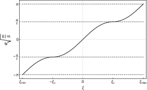
Figure 3: Plot of the $\varphi=G(\xi)$ function composed of two branches: $G_{+}(\xi)$ for $\xi\in[-\xi_{c},\xi_{c}]$ and $G_{-}(\xi)$ for $\xi\in(\xi_{\text{min}},-\xi_{c})\cup(\xi_{c},\xi_{\text{max}}]$. We see that this function is increasing monotonically and covers the whole range of variability of $\varphi$.

Let us first consider the positive branch. Choosing $G_{+}(0)=0$ and $G^{\prime}_{+}(0)=1$ so that in a vicinity of $\xi=0$ we have $\varphi\approx\xi$, we find that the solution to the Eq. (61) takes the form,

$$G_{+}(\xi)=2\sqrt{\frac{S}{m}}\,{\rm am}\left(\sqrt{\frac{m}{S}}\,\frac{\xi}{2}\Big{|}2\right),$$

$$|\xi|\leq 2\sqrt{\frac{S}{m}}\,F\left(\frac{\pi}{4}\Big{|}2\right):=\xi_{c}\,,$$ (64)

where ${\rm am}(u|n)$ is the Jacobi amplitude function, and $F(x|n):=\int_{0}^{x}\frac{d\theta}{\sqrt{1-n\sin^{2}\theta}}$ is the elliptic integral of the first kind. They are known to satisfy the relation if $x={\rm am}(u|n)$, then $u=F(x|n)$. Moreover, the critical value of $|\xi|=:\xi_{c}$ corresponds to the limiting values of $|\varphi|=\frac{\pi}{2}\sqrt{\frac{S}{m}}$.

In the negative branch, assuming the boundary conditions $G_{-}(\pm\xi_{c})=\pm\frac{\pi}{2}\sqrt{\frac{S}{m}}$, we find the following solution to Eq. (61):

$$G_{-}(\xi)=\left\{\begin{array}[]{ccc}2\sqrt{\frac{S}{m}}\,{\rm am}\left(\frac{i}{2}\left(\xi-\left(1+i\right)\xi_{c}\right)\sqrt{\frac{m}{S}}\Big{|}2\right)&\text{for}&\xi\in(\xi_{c},\xi_{\text{max}}]\\ 2\sqrt{\frac{S}{m}}\,{\rm am}\left(\frac{i}{2}\left(\xi+\left(1+i\right)\xi_{c}\right)\sqrt{\frac{m}{S}}\Big{|}2\right)&\text{for}&\xi\in(\xi_{\text{min}},-\xi_{c})\end{array}\right..$$ (65)

Despite the presence of imaginary factors $i$, the above functions are real valued. The minimal and maximal values of $\xi$ are

$$\xi_{\text{min}} =-\xi_{c}+2i\left(F\left(\frac{\pi}{4}\Big{|}2\right)-F\left(\frac{\pi}{2}\Big{|}2\right)\right)\sqrt{\frac{S}{m}}\,,$$ (66)

$$\xi_{\text{max}} =\xi_{c}-2i\left(F\left(\frac{\pi}{4}\Big{|}2\right)-F\left(\frac{\pi}{2}\Big{|}2\right)\right)\sqrt{\frac{S}{m}}\,.$$ (67)

The $\varphi=G(\xi)$ function in the full range of variability of its argument (covering the $G_{+}(\xi)$ and $G_{-}(\xi)$ branches) is plotted in Fig. 3.

In the low-energy limit, in which gradients are small, the DBI-like action [Eq. (62)] takes the approximate form

$$S_{\xi}=\int\!d^{4}x\sqrt{q}\,N\left(\mp\frac{1}{2}g^{\mu\nu}\partial_{\mu}\xi\partial_{\nu}\xi+\frac{1}{f(\xi)}\right)+\text{h.o.t.}\,,$$ (68)

where the $\mp$ sign refers to the ${\cal F}_{+}$ or ${\cal F}_{-}$ sector, respectively.

In such a case, the functional $f(\xi)$ plays the role of the effective potential,

$$U(\xi):=-\frac{1}{f(\xi)}\approx-mS+\frac{1}{2}m^{2}\xi^{2}-\frac{m^{3}}{8S}\xi^{4}+\mathcal{O}(\xi^{6})\,.$$ (69)

Then the mass of the field $\xi$ is indeed represented by the scalar $m$. The quartic self interaction term is of the order $\mathcal{O}(1/S)$ as the neglected higher order kinetic term.

Finally, performing the large $S$ expansion of the action in Eq. (59) with the functional $f(\xi)$ given by the expression in Eq. (63), we obtain,

$$S_{\xi} =mS\int\!d^{4}x\sqrt{q}N+\int\!d^{4}x\sqrt{q}\,N\left(\mp\frac{1}{2}g^{\mu\nu}\partial_{\mu}\xi\partial_{\nu}\xi-\frac{1}{2}m^{2}\xi^{2}\right)$$

$$+\frac{1}{2mS}\int\!d^{4}x\sqrt{q}\,N\left(-\frac{1}{2}g^{\mu\nu}\partial_{\mu}\xi\partial_{\nu}\xi-\frac{1}{2}m^{2}\right)\left(+\frac{1}{2}g^{\mu\nu}\partial_{\mu}\xi\partial_{\nu}\xi-\frac{1}{2}m^{2}\right)+\mathcal{O}(1/S^{2})\,.$$ (70)

This action gives the following equations of motion for $\xi$,

$$\begin{split}0&=\mp\frac{1}{\sqrt{-g}}\partial_{\nu}\left[\sqrt{-g}g^{\mu\nu}\partial_{\mu}\xi\right]+m^{2}\xi\\ &+\frac{1}{mS}\Bigg{[}\frac{1}{\sqrt{-g}}\partial_{\nu}\left[\sqrt{-g}\left(\frac{1}{2}g^{\mu\nu}\partial_{\mu}\xi\partial_{\nu}\xi+\frac{1}{2}m^{2}\xi^{2}\right)g^{\alpha\beta}\partial_{\alpha}\xi\right]-\left[\frac{1}{2}g^{\mu\nu}\partial_{\mu}\xi\partial_{\nu}\xi+\frac{1}{2}m^{2}\xi^{2}\right]m^{2}\xi\Bigg{]}+\mathcal{O}(S^{-2})\,,\end{split}$$ (71)

corresponding to the sectors, ${\cal F}_{+}$ and ${\cal F}_{-}$, respectively. To unify the notation, the identity, $N\sqrt{q}=\sqrt{-g}$, was used. The first two terms contribute to the standard wave equation for the Klein-Gordon on curved spacetime, while the terms of order $\mathcal{O}(S^{-1})$ specify the nonlinear corrections.

VII Cosmological implications

What would a continuous spin system embedded into spacetime imply on its dynamics? In the previous section, a parallel between the general relativistic spin action and the DBI-type action has been established, which permits one to make some predictions toward this direction, being of particular relevance in the cosmological context.

This is because, since a few decades, works on string theory led to a renewed interest concerning the DBI action due to its link with the $D$-brane models [32]. Imposing the DBI action [Eq. (59)] to be real requires the square root $\sqrt{1-f(\xi)\,g^{\mu\nu}\partial_{\mu}\xi\partial_{\nu}\xi}$ to be real valued. Under this condition – and considering negative $f$ function, an upper bound on the scalar field velocity $|\dot{\xi}|$ is predicted. This upper bound is responsible for the so-called $D$-cceleration mechanism and can be shown to introduce naturally a slow-roll inflation [33], with promising predictions on the non-Gausiannity of the power spectrum of the CMB [34]. This sections aims to investigate briefly if such cosmological features are also implied by our model, while we keep a more detailed analysis for forthcoming publication.

VII.1 Stress-energy tensor

The stress-energy tensor for the scalar field $\xi$ with the action [Eq. (62)] is

$$T^{\mu\nu} :=\frac{2}{\sqrt{-g}}\frac{\delta S_{\xi}}{\delta g_{\mu\nu}}$$

$$=\frac{g^{\mu\nu}(1-|f|\,\partial_{\delta}\xi\partial^{\delta}\xi)+|f|\partial^{\mu}\xi\partial^{\nu}\xi}{f\sqrt{1-|f|\,\partial_{\delta}\xi\partial^{\delta}\xi}}\,.$$ (72)

From here, energy density ($\rho$) and pressure ($p$) of the scalar field can be extracted using the standard expression, valid for the thermal equilibrium case,

$$T^{\mu\nu}=(\rho+p)u^{\mu}u^{\nu}+pg^{\mu\nu},$$ (73)

where $u^{\mu}$ is a four-velocity, satisfying the normalization condition $g_{\mu\nu}u^{\mu}u^{\nu}=-1$.

Because we are interested in cosmological consequences, let us from now on specify the metric to be that of isotropic, homogeneous, and flat Friedmann-Lemaître-Robertson-Walker (FLRW) models with the time gauge fixed by choosing the lapse function to be $N=1$. In this case, we have $g_{\mu\nu}=(-1,a^{2}\delta_{ij})$, $g^{\mu\nu}=(-1,\delta^{ij}/a^{2})$, where $a$ denotes the scale factor. For this metric, in the comoving reference frame, the well normalized four-velocity vector takes the form $u^{\mu}=(1,0,0,0)$. In consequence, only diagonal elements of the stress-energy tensor [Eq. (73)] survive, leading to the relations: $\rho=T^{00}$ and $p=\frac{1}{3}g_{ij}T^{ij}$.

In consequence, for the isotropic and homogeneous background geometry, the stress-energy tensor of the (test) field $\xi$, given by Eq. (72), leads to the following expressions for energy density and pressure:

$$\begin{split}\rho&=-\frac{\alpha}{f}\,,\\ p&=\frac{1}{3a^{2}}\,{\rm sgn}(f)\alpha(\nabla\xi)^{2}+\frac{1}{\alpha f}\,,\end{split}$$ (74)

and

$$\alpha(\xi,\dot{\xi}):=\frac{1}{\sqrt{1-|f(\xi)|\,g^{\mu\nu}\partial_{\mu}\xi\partial_{\nu}\xi}}\,.$$ (75)

We emphasize that, because of the sign difference, this function does not correspond to the $\gamma$ Lorentz-like factor for $D$-branes in general.

In the large spin limit when $\xi\rightarrow 0$, we obtain,

$$\rho =\frac{1}{2}\dot{\xi}^{2}-\frac{1}{2a^{2}}(\nabla\xi)^{2}-mS+\frac{1}{2}m^{2}\xi^{2}+\mathcal{O}(1/S)\,,$$ (76)

$$p =\frac{1}{2}\dot{\xi}^{2}-\frac{1}{6a^{2}}(\nabla\xi)^{2}+mS-\frac{1}{2}m^{2}\xi^{2}+\mathcal{O}(1/S)\,.$$ (77)

The leading order terms are in agreement with the standard expressions for the Klein-Gordon scalar field. However, because of the constant contribution $mS$, the large spin limit ($S\rightarrow\infty$) leads to divergences. The role of this constant is not specified at this level. One possibility to avoid the unphysical behavior is to subtract the $mS$ term from the action [(62)] such that the new renormalised version is

$$\tilde{S}_{\xi} =\int\!d^{4}x\sqrt{q}\,N\ \frac{1}{f(\xi)}\sqrt{1-|f(\xi)|\,g^{\mu\nu}\partial_{\mu}\xi\partial_{\nu}\xi}$$

$$-mS\int\!d^{4}x\sqrt{q}\,N\,.$$ (78)

VII.2 Cosmological evolution

In the considered case of the FLRW cosmology, the dynamics of a universe is entirely described by the Friedmann equations,

$$\begin{split}H^{2}&:=\left(\frac{\dot{a}}{a}\right)^{2}=\frac{8\pi G}{3}\rho,\\ \dot{H}+H^{2}&:=\frac{\ddot{a}}{a}=-\frac{4\pi G}{3}\left(\rho+3p\right),\end{split}$$ (79)

where $H$ is the Hubble factor, and $\ddot{a}/a$ is quantifying acceleration rate of expansion.

Expressing the equation of state in the form

$$p=w\rho,$$ (80)

where $w$ is a function being a constant for the special case of barotropic fluid, it is convenient to discriminate between different types of evolution of a universe. Namely, it follows from the second Friedmann equation [Eq. (79)] that for a positive energy density,

$$\begin{split}w&>-1/3\Longrightarrow\ddot{a}<0\,,\\ w&<-1/3\Longrightarrow\ddot{a}>0\,,\\ w&=-1/3\Longrightarrow\ddot{a}=0\,,\end{split}$$ (81)

while a negative energy density would imply change of sign for the acceleration in the expressions above. However, the latter case is physical only if appropriate modifications to the first Friedmann equation [Eq. (79)] are present, ensuring that $H^{2}\geq 0$.

Employing Eq. (74), the homogeneous contributions from the scalar field $\xi$ to energy density and pressure are

$$\begin{split}\rho&=-\frac{\alpha}{f}\,,\\ p&=\frac{1}{f\alpha}\,.\end{split}$$ (82)

One can immediately notice that the two cases where the energy density is positive or negative correspond to the two hemispheres of the phase space where, respectively, $\varphi\in{\cal F}_{-}$ or $\varphi\in{\cal F}_{+}$.

We remind that, in Sec. III, the Lagrangian of our model was shown to match with that of a scalar field in the large spin limit for the second case $\varphi\in{\cal F}_{+}$. We will, however, consider both possibilities in the following analysis.

More broadly, on both hemispheres, the parameter $w$ takes the form,

$$w=-\frac{1}{\alpha^{2}}=-1-|f(\xi)|\dot{\xi}^{2}\leq-1\,,$$ (83)

where in the considered FLRW case, $\alpha$ reduces to

$$\alpha(\xi,\dot{\xi}):=\frac{1}{\sqrt{1+|f(\xi)|\dot{\xi}^{2}}}\,.$$ (84)

It is interesting to notice that in the Euclidean case (i.e., after the Wick rotation), the $\alpha$ function transforms precisely to the $\gamma$ Lorentz-like factor in DBI theory.

While Eq. (83) has similar functional form as in the usual DBI cosmology [33], here, we have $\alpha\leq 1$ always. This ensures that $w\leq-1$, and, in consequence the expansion of a universe is continually accelerated if $\rho>0$. This behavior is similar to the one know from the case of phantom cosmologies [49]. Furthermore, since $w<-1/3$, the more a universe expands, the more $\rho$ increases. In consequence, the more $\rho$ increases, the faster a universe expands, thus engendering internal inflation as soon as $\dot{a}>0$. The $D$-cceleration leading to slow-roll inflation is, therefore, excluded by our model.

On the other hand, assuming now that $f$ is positive ($\varphi\in\mathcal{F}_{+}$) such that the energy density is negative definite, a similar reasoning leads to the conclusion that the expansion is decelerated, which is, by definition, incompatible with an inflationary scenario.

One could, however, argue that the flatness and horizon problems can still be solved without the need for an inflationary phase. The other common solution requires a recollapse phase and refers to an ekpyrotic or cyclic universe [50].

Alternatively, both problems are solved through the emission of tachyacoustic perturbations, which also happen to be scale invariant [51]. One can indeed observe that the speed of adiabatic waves for our model is larger than the speed of light in vacuum [52, 34],

$$c_{s}^{2}=\frac{1}{\alpha^{2}}=1+|f(\xi)|\dot{\xi}^{2}\geq 1.$$ (85)

It is important to notice that these tachyacoustic perturbations for $k$-essence models [53] do not violate causality [54] (see [51] for an application of the proof to the DBI case).

Closing the discussion on the inflationary phase, the obtained DBI-like action may imply broader phenomenology and be considered as a candidate for dark energy [55]. Furthermore, worth stressing is also the relation to the Chaplygin gas models and tachyon condensate. Another important property is that the DBI-type $k$-essence models, to which our model belongs, have a unique property from the viewpoint of the problem of introducing time in gravity, by virtue of the Brown-Kuchar mechanism [56].

VIII Summary

In this article, the general-relativistic model of a continuous spin system has been constructed. It has been derived as a generalization of a system of spins (magnetic moments) precessing in a constant magnetic field. An essential step was the application of the semiclassical version of the Holstein-Primakoff transformation, which allowed us to relate phase space of a spin field with phase space of a scalar field, so that the Poisson bracket on the latter remains canonical. The transformation is an example of a general procedure introduced recently in the context of nonlinear field space theories (NFSTs).

The construction discussed in this article is not unique, and the method can be used to obtain other theories of spin fields on curved spacetimes. However, the considered case is special because of a few reasons. First, the investigated model reduces to the relativistic massive scalar field theory (Klein-Gordon field) in the large spin limit. Second, in the large mass limit and in the vicinity of a ground state, the model reduces to the continuous Ising model coupled to an external constant transversal magnetic field. Third, the model is equivalent to a concrete realisation of the DBI-type $k$-essence scalar field theory, with the form of the $f(\xi)$ function predicted by the model.

The third point is especially interesting since it indicates that there is a certain relation between spin fields and the Dirac-Born-Infeld theory. The spin field is, in turn, an example of NFST with the compact phase space. Actually, one of the motivations behind proposing the NFST program was to impose constraints on the field values in the spirit of the original Born-Infeld theory. However, in the case of NFST, this is done by introducing nonlinearity to the field phase space. The results of our investigations confirm that some compact phase space realisations of NFST may be equivalent to the DBI-type scalar field theories. This also shows a possible connection between compact phase spaces and string theory, in the context of which, the DBI models have been considered in the recent literature. Furthermore, reduction to the DBI-type $k$-essence opens a possibility of making phenomenological predictions, especially in cosmology [34], which has been preliminarily explored here.

The approach introduced in this paper provides a consistent method of coupling a spin field to gravity, which may be of relevance not only at the classical but also at the quantum level. While one possibility given by our framework is coupling a spin field to quantum gravity, not less interesting is the analysis of quantum spin systems on curved backgrounds. Therefore, the considered model and the whole framework may find application in the domain of quantum many-body systems on curved spacetimes and the relativistic quantum information theory [57]. This may be relevant, e.g., in theoretical description of such astrophysical objects as neutron stars, quark stars, or white dwarfs, where both quantum and gravitational effects (but not quantum-gravitational) are relevant. For this purpose, quantization of the spin field considered in the paper has to be performed, which is a challenge that interested readers are encouraged to take.

Appendix A semiclassical Holstein-Primakoff transformation

The Holstein-Primakoff transformation [16] expresses the spin operators [generating the $\mathfrak{su}(2)$ algebra] in terms of the bosonic creation and annihilation operators. Restricting our interest to specific irreducible representations amounts to a truncation of the infinite-dimensional Hilbert space to a finite one. The transformation has the form (in the Cartan-Weyl basis $\hat{S}^{\pm}:=\hat{S}^{x}\pm i\hat{S}^{y}$, $\hat{S}^{z}$),

$$\begin{split}\hat{S}^{z}&=\hbar\left(s-\hat{a}^{\dagger}\hat{a}\right)\,,\\ \hat{S}^{+}&=\hbar\sqrt{2s}\,\sqrt{1-\frac{\hat{a}^{\dagger}\hat{a}}{2s}}\,\hat{a}\,,\\ \hat{S}^{-}&=\hbar\sqrt{2s}\,\hat{a}^{\dagger}\sqrt{1-\frac{\hat{a}^{\dagger}\hat{a}}{2s}}\,,\end{split}$$ (86)

where the ladder operators satisfy the bosonic commutator, $\left[\hat{a},\hat{a}^{\dagger}\right]=1$. We compute the semiclassical limit of this algebra in the canonical manner, according to [58]. The relevant quantities in this limit are the expectation values of the considered operators, $\langle\hat{S}^{(z,\pm)}\rangle$.

The expectation value of the commutator entails the form of the Poisson bracket,

$$\left\{\langle\hat{A}\rangle,\langle\hat{B}\rangle\right\}=\frac{1}{i\hbar}\left\langle\left[\hat{A},\hat{B}\right]\right\rangle,$$ (87)

so that, in particular, $\left\{a,a^{\dagger}\right\}=-\frac{i}{\hbar}$, where $a\equiv\langle\hat{a}\rangle$ and $a^{\dagger}\equiv\langle\hat{a}^{\dagger}\rangle$. Defining $S:=\hbar s$ and $N:=\langle\hat{a}^{\dagger}\rangle\langle\hat{a}\rangle$, we obtain the semiclassical expressions for spin variables in terms of bosonic variables,

$$\begin{split}S^{z}&=S-\hbar N+O(\hbar^{2})\,,\\ S^{+}&=\sqrt{\hbar}\,a\sqrt{2S-\hbar N}+O(\hbar^{2})\,,\\ S^{-}&=\sqrt{\hbar}\,a^{\dagger}\sqrt{2S-\hbar N}+O(\hbar^{2})\,.\end{split}$$ (88)

The correction terms come from the quantum fluctuations and from ordering ambiguities, which can be neglected in the semiclassical regime. Generators of the $\mathfrak{su}(2)$ algebra in the standard basis (i.e., $S^{x}$, $S^{y}$, $S^{z}$) are then given by,

$$\begin{split}S^{z}&=S-\hbar N\,,\\ S^{x}&=\frac{\sqrt{\hbar}}{2}\left(a+a^{\dagger}\right)\sqrt{2S-\hbar N}\,,\\ S^{y}&=\frac{\sqrt{\hbar}}{2i}\left(a-a^{\dagger}\right)\sqrt{2S-\hbar N}\,.\end{split}$$ (89)

They satisfy the $\mathfrak{su}(2)$ Lie algebra bracket, given by the Poisson bracket [Eq. (87)] we just defined.

At the next step, we introduce an action variable, $J:=\hbar N$, which is canonically conjugate to some angle variable, $\theta$. The canonical structure implies that both $a$ and $a^{\dagger}$ depend on $\theta$, and the form of this dependence can be determined by considering the following brackets,

$$\begin{split}\left\{a,J\right\}&=\frac{\partial a}{\partial\theta}=-ia\,,\\ \left\{a^{\dagger},J\right\}&=\frac{\partial a^{\dagger}}{\partial\theta}=ia^{\dagger}\,.\end{split}$$ (90)

The solution of the above system is

$$\begin{split}a&=\sqrt{\frac{J}{\hbar}}\,{\rm e}^{-i\theta}\,,\\ a^{\dagger}&=\sqrt{\frac{J}{\hbar}}\,{\rm e}^{i\theta}\,,\end{split}$$ (91)

where $\left\{\theta,J\right\}=1$, and the constants of integration were fixed by requiring $a^{\dagger}a=N$. Expressing the formulae in Eq. (89) in terms of the canonical variables, we ultimately obtain

$$\begin{split}S^{z}&=S-J\,,\\ S^{x}&=\cos{(\theta)}\sqrt{J(2S-J)}\,,\\ S^{y}&=-\sin{(\theta)}\sqrt{J(2S-J)}\,.\end{split}$$ (92)

Last, to recover the parametrization selected in this paper, we perform the subsequent linear canonical transformation

$$\begin{split}\varphi&=-R_{\varphi}\theta\,,\\ \pi_{\varphi}&=R_{\pi}-\frac{J}{R_{\varphi}}\,.\end{split}$$ (93)

Recalling the relation [Eq. (9)] and either moving the tensor codensity encoded in $1/\sqrt{q}$ into the Levi-Civita symbol [compare with the expression (10)] or setting the flat space limit, restricting to $q=1$, and simplifying the relation (9) to $R_{\varphi}R_{\pi}=S$, we obtain the parametrization postulated in Eqs. (5)–(7). This confirms that our parametrization is the semiclassical analog of the Holstein-Primakoff transformation.

References

- [1] E. Lieb, T. Schultz and D. Mattis, Ann. Phys. N.Y. 16, 407 (1961).
- [2] J. Hubbard, ”Electron Correlations in Narrow Energy Bands”. Proceedings of the Royal Society of London 276 (1365): 238-257 (1963).
- [3] J. Kosterlitz and D. Thouless, “Ordering, metastability and phase transitions in two-dimensional systems,” J. Phys. C 6, 1181 (1973).
- [4] H. Muntinga, et al., “Interferometry with Bose-Einstein Condensates in Microgravity,” Phys. Rev. Lett. 110, 093602 (2013) [arXiv:1301.5883 [physics.atom-ph]].
- [5] D. Becker, M. D. Lachmann, S. T. Seidel, et al., Space–borne Bose–Einstein condensation for precision interferometry. Nature 562, 391 (2018).
- [6] D. C. Aveline, J. R. Williams, E. R. Elliott, et al., “Observation of Bose–Einstein condensates in an Earth-orbiting research lab,” Nature 582, 193 (2020).
- [7] M. Gell-Mann and M. Levy, “The axial vector current in beta decay,” Nuovo Cim. 16, 705 (1960).
- [8] E. Witten, “Nonabelian Bosonization in Two-Dimensions,” Commun. Math. Phys. 92, 455 (1984).
- [9] H. B .Nielsen and D. Rohrlich, “A path integral to quantize spin,” Nucl. Phys. B 299, 471 (1988).
- [10] A. Alekseev, L. Faddeev and S. Shatashvili, “Quantization of symplectic orbits of compact Lie groups by means of the functional integral,” J. Geom. Phys. 5, 391 (1988).
- [11] P. Wiegmann, “Multivalued functionals and geometrical approach for quantization of relativistic particles and strings,” Nucl. Phys. B 323, 311 (1989).
- [12] T. Rempel and L. Freidel, “Interaction vertex for classical spinning particles,” Phys. Rev. D 94, 044011 (2016).
- [13] T. Rempel and L. Freidel, “Bilocal model for the relativistic spinning particle,” Phys. Rev. D 95, 104014 (2017).
- [14] A. P. Balachandran, G. Marmo, B. S. Skagerstam and A. Stern, “Spinning particles in general relativity,” Phys. Lett. B 89, 199 (1980).
- [15] A. A. Kirillov, “Lectures on the Orbit Method,” American Mathematical Society, Providence 2004.
- [16] T. Holstein and H. Primakoff, “Field Dependence of the Intrinsic Domain Magnetization of a Ferromagnet,” Phys. Rev. 58, 1098 (1940).
- [17] F. J. Dyson, “General theory of spin-wave interactions,” Phys. Rev. 102, 1217-1230 (1956).
- [18] F. J. Dyson, “Thermodynamic Behavior of an Ideal Ferromagnet,” Phys. Rev. 102, 1230-1244 (1956).
- [19] S. V. Maleev, “Scattering of Slow Neutrons in Ferromagnets,” JETP, Vol. 6, No. 4, 776 (1958).
- [20] P. Jordan, “Der Zusammenhang der symmetrischen und linearen Gruppen und das Mehrkörperproblem,” Zeitschrift für Physik 94, Issue 7-8, 531-535 (1935).
- [21] J. Schwinger, “On Angular Momentum,” Unpublished Report, Harvard University, Nuclear Development Associates, Inc., United States Department of Energy (through predecessor agency the Atomic Energy Commission), Report Number NYO-3071 (1952).
- [22] D. D. Stancil and A. Prabhakar, “Spin Waves: Theory and Applications,” Springer, Boston, MA (2009).
- [23] J. Mielczarek and T. Trześniewski, “The Nonlinear Field Space Theory,” Phys. Lett. B 759, 424 (2016) [arXiv:1601.04515 [hep-th]].
- [24] M. Born and L. Infeld, “Foundations of the New Field Theory,” Proc. R. Soc. Lond. A 144, 425 (1934).
- [25] M. Born, “A Suggestion for Unifying Quantum Theory and Relativity,” Proc. R. Soc. Lond. A 165, 291 (1938).
- [26] G. Amelino-Camelia, L. Freidel, J. Kowalski-Glikman and L. Smolin, “The principle of relative locality,” Phys. Rev. D 84, 084010 (2011) [arXiv:1101.0931 [hep-th]].
- [27] L. Freidel, R. G. Leigh and D. Minic, “Metastring theory and modular spacetime,” JHEP 06, 006 (2015) [arXiv:1502.08005 [hep-th]].
- [28] A. Ashtekar, S. Fairhurst, and J. L. Willis, “Quantum gravity, shadow states and quantum mechanics,” Class. Quantum Grav. 20, 1031 (2003).
- [29] J. Mielczarek, “Spin-Field Correspondence,” Universe 3, 29 (2017) [arXiv:1612.04355 [hep-th]].
- [30] J. Bilski, S. Brahma, A. Marcianò and J. Mielczarek, “Klein-Gordon field from the XXZ Heisenberg model,” Int. J. Mod. Phys. D 28, 1950020 (2018) [arXiv:1708.03207 [hep-th]].
- [31] T. Trześniewski, “Nonlinear Field Space Theory and Quantum Gravity,” Acta Phys. Pol. B Proc. Suppl. 10, 329 (2017) [arXiv:1701.06865 [hep-th]].
- [32] R. Leigh, “Dirac-Born-Infeld Action from Dirichlet Sigma Model,” Mod. Phys. Lett. A 4, 2767 (1989).
- [33] E. Silverstein and D. Tong, “Scalar speed limits and cosmology: Acceleration from -cceleration,” Phys. Rev. D 70 (2004), 103505 [hep-th/0310221].
- [34] M. Alishahiha, E. Silverstein and D. Tong, “DBI in the sky,” Phys. Rev. D 70, 123505 (2004) [hep-th/0404084].
- [35] D. Artigas, J. Mielczarek and C. Rovelli, “A minisuperspace model of compact phase space gravity,” Phys. Rev. D 100, 043533 (2019) [arXiv:1904.11338 [gr-qc]].
- [36] D. Artigas, S. Crowe and J. Mielczarek, “Quantum fluctuations of the compact phase space cosmology,” arXiv:2003.08129 [gr-qc].
- [37] I. Bailey and W. Israel, “Lagrangian Dynamics of Spinning Particles and Polarized Media in General Relativity,” Commun. Math. Phys. 42, 65 (1975).
- [38] M. Blagojević and F. W. Hehl, “Gauge Theories of Gravitation,” Imperial College Press, London 2012 [arXiv:1210.3775 [gr-qc]].
- [39] A. Trautman, “Einstein-Cartan theory,” in: “Encyclopedia of Mathematical Physics”, eds. J.-P. Francoise, G.L. Naber and S.T. Tsou, Elsevier 2006 [gr-qc/0606062].
- [40] S. Tomonaga, “Remarks on Bloch’s Method of Sound Waves applied to Many-Fermion Problems,” Prog. Theor. Phys. 5, 544 (1950).
- [41] D. C. Mattis and E. H. Lieb, “Exact solution of a many fermion system and its associated boson field,” J. Math. Phys. 6, 304 (1965).
- [42] J. M. Luttinger, “An Exactly Soluble Model of a Many-Fermion System,” J. Math. Phys. 4, 1154 (1963).
- [43] V. F. Mukhanov, H. A. Feldman and R. H. Brandenberger, “Theory of cosmological perturbations. Part 1. Classical perturbations. Part 2. Quantum theory of perturbations. Part 3. Extensions,” Phys. Rept. 215, 203 (1992).
- [44] J. Mielczarek and T. Trześniewski, “Nonlinear Field Space Cosmology,” Phys. Rev. D 96, 043522 (2017) [arXiv:1704.01934 [gr-qc]].
- [45] A. Angelucci and R. Link, “Graded holstein-primakoff transformations and the semiclassical limit of strongly correlated electron systems,” Phys. Rev. B 46, 3089 (1992).
- [46] C. W. Misner, K. S. Thorne, and J. A. Wheeler, “Gravitation,” W.H. Freeman and Co., San Francisco 1973.
- [47] P. Pfeuty, The one-dimensional Ising model with a transverse field Annals of Physics, Volume 57, Issue 1, (1970).
- [48] T. Kadowaki, H. Nishimori, Quantum Annealing in the Transverse Ising Model Phys. Rev. E 58, 5355 (1998).
- [49] R. Caldwell, “A Phantom menace?,” Phys. Lett. B 545, 23 (2002) [astro-ph/9908168].
- [50] J. L. Lehners, “Ekpyrotic and Cyclic Cosmology,” Phys. Rept. 465, 223 (2008) [arXiv:0806.1245 [astro-ph]].
- [51] D. Bessada, W. H. Kinney, D. Stojkovic and J. Wang, “Tachyacoustic Cosmology: An Alternative to Inflation,” Phys. Rev. D 81, 043510 (2010) [arXiv:0908.3898 [astro-ph.CO]].
- [52] J. Garriga and V. F. Mukhanov, “Perturbations in k-inflation,” Phys. Lett. B 458, 219 (1999) [hep-th/9904176].
- [53] C. Armendáriz-Picón, T. Damour and V. F. Mukhanov, “k - inflation,” Phys. Lett. B 458, 209 (1999) [hep-th/9904075].
- [54] E. Babichev, V. Mukhanov and A. Vikman, “-Essence, superluminal propagation, causality and emergent geometry,” JHEP 02, 101 (2008) [arXiv:0708.0561 [hep-th]].
- [55] J. Martin and M. Yamaguchi, “DBI-essence,” Phys. Rev. D 77, 123508 (2008) [arXiv:0801.3375 [hep-th]].
- [56] T. Thiemann, “Solving the Problem of Time in General Relativity and Cosmology with Phantoms and -Essence,” astro-ph/0607380.
- [57] R. B. Mann and T. C. Ralph, “Relativistic quantum information,” Class. Quantum Grav. 29, 220301 (2012).
- [58] M. Bojowald and A. Skirzewski, “Effective equations of motion for quantum systems,” Rev. Math. Phys. 18, 713 (2006).