SUPER-II: Spatially resolved ionized gas kinematics and scaling relations in $z\sim$ 2 AGN host galaxies

Abstract

Aims. The SINFONI survey for Unveiling the Physics and Effect of Radiative feedback (SUPER) aims at tracing and characterizing ionized gas outflows and their impact on star formation in a statistical sample of X-ray selected Active Galactic Nuclei (AGN) at z$\sim$2. We present the first SINFONI results for a sample of 21 Type-1 AGN spanning a wide range in bolometric luminosity (log $\mathrm{L_{bol}}$ = 45.4–47.9 erg/s). The main aims of this paper are determining the extension of the ionized gas, characterizing the occurrence of AGN-driven outflows, and linking the properties of such outflows with those of the AGN.

Methods. We use Adaptive Optics-assisted SINFONI observations to trace ionized gas in the extended narrow line region using the [O iii] $\lambda$5007 line. We classify a target as hosting an outflow if its non-parametric velocity of the [O iii] line, $\mathrm{w_{80}}$, is larger than 600 km/s. We study the presence of extended emission using dedicated point-spread function (PSF) observations, after modelling the PSF from the Balmer lines originating from the Broad Line Region.

Results. We detect outflows in all the Type-1 AGN sample based on the $\mathrm{w_{80}}$ value from the integrated spectrum, which is in the range $\sim$650–2700 km/s. There is a clear positive correlation between $\mathrm{w_{80}}$ and the AGN bolometric luminosity (99% correlation probability), but a weaker correlation with the black hole mass (80% correlation probability). A comparison of the PSF and the [O iii] radial profile shows that the [O iii] emission is spatially resolved for $\sim$35% of the Type-1 sample and the outflows show an extension up to $\sim$6 kpc. The relation between maximum velocity and the bolometric luminosity is consistent with model predictions for shocks from an AGN driven outflow. The escape fraction of the outflowing gas increase with the AGN luminosity, although for most galaxies, this fraction is less than 10%.

1 Introduction

Quasars represent some of the most energetic sources in the Universe which may regulate the gas flows in and out their host galaxies. A manifestation of the impact that super-massive black holes (SMBHs) may have on the galaxy are the well established black hole-host galaxy scaling relations such as the BH mass, $\mathrm{M_{BH}}$, vs. galaxy mass, $\mathrm{M_{\ast}}$, (e.g. Magorrian et al., 1998; Läsker et al., 2016; Schutte et al., 2019) and the $\mathrm{M_{BH}}$ vs. stellar velocity dispersion, $\sigma_{\ast}$, relations (e.g. Gebhardt et al., 2000; Batiste et al., 2017; Caglar et al., 2020).

One promising physical phenomenon to link the growth of the SMBH and the evolution of its host is that of fast winds launched from the AGN accretion disk (¿1000 km/s, e.g. King, 2003; Begelman, 2003; Menci et al., 2008; Zubovas & King, 2012; Faucher-Giguère & Quataert, 2012; Choi et al., 2014; Nims et al., 2015; Hopkins et al., 2016). These winds are hypothesized to shock against the surrounding gas and drive outflows that propagate out to large distances from the AGN, heat the interstellar medium (ISM) and potentially eject large amount of gas out of the system (e.g. Ishibashi & Fabian, 2016; Zubovas, 2018). Such fast winds are now observed in a vast number of AGN host galaxies at both low as well as high redshift, in different phases of gas - neutral phase using sodium absorption lines (e.g. Krug et al., 2010; Rupke & Veilleux, 2011; Cazzoli et al., 2016; Concas et al., 2019; Roberts-Borsani, 2020), cold molecular gas phase using different transitions of CO, HCN and [C ii] for instance (e.g. García-Burillo et al., 2014; Tadhunter et al., 2014; Feruglio et al., 2017; Aladro et al., 2018; Michiyama et al., 2018; Zschaechner et al., 2018; Aalto et al., 2019; Husemann et al., 2019; Cicone et al., 2020; Veilleux et al., 2020), warm and hot molecular gas phase using transitions in the mid- to near-infrared (Veilleux et al., 2009; Davies et al., 2014; Hill & Zakamska, 2014; Riffel et al., 2015; Emonts et al., 2017; May et al., 2018; Petric et al., 2018; Riffel et al., 2020), and ionized gas phase observed using the rest-frame optical emission lines such as the forbidden transitions of [O iii] $\lambda$5007 (e.g. Harrison et al., 2014; Kakkad et al., 2016; Zakamska et al., 2016; Fiore et al., 2017; Venturi et al., 2018; Baron & Netzer, 2019; Coatman et al., 2019; Förster Schreiber et al., 2019). Due to the higher surface brightness of the ionized gas traced by the forbidden transition [O iii] $\lambda$5007 relative to other optical transitions (e.g. [O ii] $\lambda$3727, [S ii] $\lambda$6716), outflows in this phase can be studied in detail for a large number of galaxies. In AGN, these forbidden ionized transitions such as [O iii] , [N ii] , and [S ii] are emitted from the Extended Narrow Line Region (ENLR), making these transitions ideal to trace kiloparsec scale ionized gas outflows from the AGN (e.g. Bennert et al., 2002; Hainline et al., 2014; Dempsey & Zakamska, 2018).

It is particularly important to study the impact that such galactic scale AGN-driven outflows may have on their host galaxies at z$\sim$2 where both the volume-averaged star-formation rate and the black hole growth rate peak (e.g. Shankar et al., 2009; Madau & Dickinson, 2014; Curran, 2019; Wilkins et al., 2019; Tacconi et al., 2020). Tremendous progress has been made through integral field unit (IFU) spectroscopy that provides spatially resolved information on the structure and extension of the outflows (e.g. Riffel et al., 2013; McElroy et al., 2015; Thomas et al., 2017; Revalski et al., 2018; Davies et al., 2019; Radovich et al., 2019). Compared to the classical narrow band imaging and/or slit spectroscopy, IFU spectroscopy allows to identify the emission from the host galaxy by subtracting the contribution from the AGN. A few IFU studies have also claimed the presence of “negative” as well as “positive” feedback in the presence of outflows i.e. ionized outflows suppressing as well as enhancing star formation within the AGN host galaxies (e.g. Cano-Díaz et al., 2012; Cresci et al., 2015; Carniani et al., 2016; Maiolino et al., 2017; Gallagher et al., 2019); however, the full intepretation of these results can be complicated by effects such as dust obscuration (e.g. Whitaker et al., 2014; Brusa et al., 2018; Scholtz et al., 2020). Most of the literature is however focused on a limited number of targets which have been pre-selected to have a higher probability to show the presence of outflows such as targets selected based on their colors, high Eddington ratio or high luminosity (e.g. Brusa et al., 2015; Perna et al., 2015; Kakkad et al., 2016; Bischetti et al., 2017; Perrotta et al., 2019). The lack of studies in a wider parameter space of the properties of the AGN and their host galaxies has so far prevented the assessment in a systematic way of a possible trend between the activity of the AGN itself (e.g. quantified by its luminosity) and the presence of outflows and consequently whether all outflows have an impact on their host galaxies. We are therefore in need of an unbiased sample where a wider range in Eddington ratio and/or bolometric luminosity is used for follow-up outflow studies.

We are currently in an era of large IFU surveys of galaxies (Sánchez et al., 2012; Bundy et al., 2015; Bryant et al., 2015; Stott et al., 2016; Förster Schreiber et al., 2018; Wisnioski et al., 2019; den Brok et al., 2020). Such statistical samples are now able to eliminate the selection biases from previous studies and give an overall picture of the ISM dynamics in the presence of both star formation and AGN processes. Recent work targeting star forming galaxies at high redshift, such as SINS/zC-SINF survey (e.g. Förster Schreiber et al., 2018; Davies et al., 2019) with SINFONI indicate that the majority of galaxies ($\sim$70%) show ordered disk rotation while the rest of the targets either show turbulent disk structure or the presence of outflows in addition to the disk rotation. The mass loading factor, which is the ratio between the outflow mass and the star formation rate, is correlated with the level of star formation within the host galaxies. The outflow fraction in SINS/zC-SINF survey is similar to KMOS-3D survey (Förster Schreiber et al., 2019) where 30% of the 599 observed targets show the presence of outflowing gas, inferred as being driven by both star formation and AGN processes. Star formation-driven winds on average show low mass loading factors when compared to the AGN-driven outflows. Coupled with the reported results in the KROSS survey (e.g. Swinbank et al., 2019), a fraction of the total gas mass is believed to escape in the low mass galaxies while all of the outflowing gas is retained in galaxies at high masses. IFU surveys of star forming galaxies come to a common conclusion that the outflow velocities are typically enhanced in the presence of an AGN.

Among AGN surveys, Leung et al. (2019) target optically-selected AGN using single-slit spectroscopy from the MOSDEF survey with bolometric luminosities in the range $\mathrm{10^{44}-10^{47}}$ erg/s at z$\sim$1.4–3.8 and find outflows in 17% of their sample of $\sim$160 AGN. Moreover, it is claimed that the ionized gas mass outflow rates correlate positively with the luminosity of the AGN, but do not depend on the galaxy stellar mass, in contrast with the findings of Förster Schreiber et al. (2018) on star forming galaxies. AGN from MOSDEF survey have higher incidence of outflows compared to redshift and stellar mass matched star forming galaxies. Although MOSDEF uses single-slit spectroscopy which, as mentioned earlier, has its own limitations, a similar result was found by Harrison et al. (2016) with the KASHz survey targeting X-ray selected AGN (2–10 keV) at z$\sim$1.1–2.5 with KMOS. The more luminous KASHz AGN are found to be more likely to host outflows with velocities ¿600 km/s and these ionized gas velocities are 10 times more prevalent in the AGN host galaxies than star forming galaxies at similar redshift and similar $\mathrm{H\alpha}\leavevmode\nobreak\$ luminosity distribution.

Most of the the current AGN surveys at z¿1 described above are based on seeing-limited observations. Consequently, both host galaxies as well as the possible outflows are usually spatially unresolved, which prevents one to have a complete understanding of how extended these outflows are. In addition, the presence of unresolved outflows implies that further assumptions have to be made (e.g. on the scale and morphology) which propagate in larger uncertainties in derived quantities such as mass loading factor and outflow kinetic power. Therefore, the way forward is to use Adaptive Optics (AO) assisted observations to resolve smaller physical scales also at z¿1 (e.g. Davies et al., 2020b). A higher spatial resolution enables one to study the impact of AGN from kiloparsec scales to Mpc scales. In this paper, we present the first results from the Type-1 AGN sample from the SINFONI survey for Unveiling the Physics and Effect of Radiative feedback (SUPER Circosta et al., 2018). SUPER is designed to overcome the limitation of low spatial resolution in order to understand the true spatial extent of outflows in AGN host galaxies at high redshift. Apart from the extension of the outflows and the ionized gas, SUPER aims at answering some of the fundamental questions such as: how prevalent are ionized outflows in X-ray selected AGN host galaxies? Do the outflow properties e.g. velocity, mass outflow rates show a correlation with those of the AGN and of the host galaxy (e.g. AGN bolometric luminosity, host star formation rate)? And if they do, what is the scaling relation between the corresponding parameters? Lastly, do these outflows have any effect on the host (e.g. its star formation rate or gas mass)?

This paper is arranged as follows: in sect. 2, we describe the sample used and its characteristics and in sect. 3 we discuss the observing strategy followed by the data reduction procedure and stacking of data cubes in sect. 4. We describe in detail the analysis procedure and the corresponding results obtained in sect. 5, discuss the implications of these results and derive scaling relations in sect. 6. Concluding remarks are reported in sect. 7.

Throughout this paper, we adopt the following $\Lambda$CDM cosmology parameters: $\mathrm{H_{o}}$ = 70 km/s, $\mathrm{\Omega_{M}}$ = 0.3, $\mathrm{\Omega_{\Lambda}}$ = 0.7.

2 Sample description

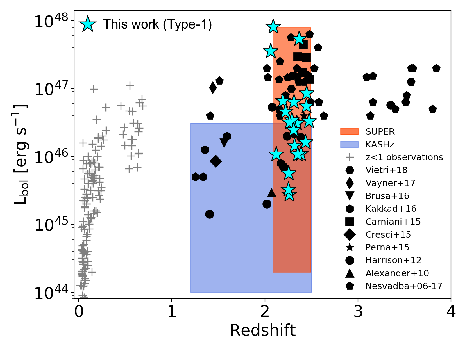
Figure 1: Past and on-going IFU surveys targeting the [O iii] $\lambda$5007 emission line to study the properties of outflows in AGN host galaxies in the $\mathrm{L_{bol}}$ vs. redshift plane. The grey data points represent surveys at $z<1$ (Husemann et al., 2013, 2014, 2017; Liu et al., 2013; Harrison et al., 2014; Karouzos et al., 2016; Bae et al., 2017; Rupke et al., 2017), while the solid black symbols are collected from $z>1$ studies (Nesvadba et al., 2006; Alexander et al., 2010; Harrison et al., 2012; Cresci et al., 2015; Carniani et al., 2015; Brusa et al., 2016; Kakkad et al., 2016; Nesvadba et al., 2017; Vayner et al., 2017; Vietri et al., 2018). The blue shaded area covers the parameter space of the KASHz survey (Harrison et al., 2016) and the red shaded area that of the overall SUPER survey (Circosta et al., 2018). This paper presents an analysis on the Type 1 sub-sample of the SUPER survey, the data points of which are shown as cyan star symbols. Adapted from Circosta et al. (2018), to whom we refer the reader for further details.

The sample presented in this paper is derived from the SUPER survey, a large program with the Spectrograph for INtegral Field Observations in the Near Infrared (SINFONI, Eisenhauer et al., 2003) mounted on the Cassegrain focus of Unit Telescope 4 (UT4) at the Very Large Telescope (VLT). We briefly discuss the overall properties of the SUPER sample in this section, in particular the Type-1 sub-sample used in this paper. For more details on sample selection and the survey characteristics we refer the reader to Circosta et al. (2018).

The SUPER survey consists of a sample of 39 AGN selected in the X-rays ($\mathrm{L_{2-10\leavevmode\nobreak\ kev}>10^{42}\leavevmode\nobreak\ erg/s}$) in the Chandra Deep Field South (e.g. Luo et al., 2017), COSMOS-Legacy (e.g. Civano et al., 2016), the wide area XMM-XXL (e.g. Georgakakis & Nandra, 2011; Liu et al., 2016; Menzel et al., 2016), and Stripe 82 X-ray (e.g. LaMassa et al., 2016) surveys and from the WISE/SDSS selected Hyper-luminous quasar sample (e.g. Bischetti et al., 2017). The X-ray selection with the luminosity cut ensures a pure AGN selection as there is no contamination from the host galaxy and/or X-ray binaries at these energies (see e.g. Brandt & Alexander, 2015; Padovani et al., 2017). The sample covers a redshift range of 2.1 – 2.5, which is the epoch of maximal activity of the volume averaged star formation in galaxies and the growth of black holes in the universe, making it ideal to study effects of radiative feedback from the black hole on the host galaxy (e.g. Madau & Dickinson, 2014). Owing to the presence of ancillary multi-wavelength data sets, we are able to derive accurate measurements of the black hole and the host galaxy properties via spectral energy distribution fitting of UV-to-FIR photometry and X-ray spectral fitting (details in Circosta et al. 2018 for the analysis of the multi-wavelength data sets and Vietri 2020 for the black hole mass estimations). Of the 39 targets, 22 were classified as Type-1 (56%) and the remaining 17 as Type-2 (44%), based on the presence or absence of broad emission lines such as MgII or CIV in the optical spectra. One target, cid_1205, which was previously reported as a Type-2 AGN in Circosta et al. (2018) is now classified as a Type-1 AGN based on the presence of BLR emission in $\mathrm{H\alpha}\leavevmode\nobreak\$ line in the K-band SINFONI spectrum. So, 23 galaxies (58%) from the SUPER sample are now classified as Type-1 AGN. The overall SUPER sample span a wide range in AGN and host galaxy properties which allows us to identify any existing correlation between the outflow properties derived from the SINFONI data and those derived from the multi-wavelength ancillary data set.

In this paper, we focus on the analysis of the H-band SINFONI data of the Type-1 targets from the SUPER survey. The selected sample in the context of other SUPER targets and on-going IFU surveys is shown as $cyan$ star symbols in Fig. 1. These targets populate the moderate-to-high luminosity range and span $\sim$2.5 order of magnitude in bolometric luminosity among the SUPER sample. We explore the following range of black hole and host galaxy properties for the spatially resolved data set presented in this paper: log M_∗/M_⊙ $\sim$10.38–11.20, SFR ¡94–686 M_⊙/yr, log L_bol/[erg/s]  $\sim$ 45.4–47.9, log M_BH/M_⊙   $\sim$8.3–10.7 and log N_H/cm^-2   ¡21.25– ¿24.1. The properties of the individual targets obtained from the SED fits and the available optical data are reported in Table 1.

3 Observations

The SUPER SINFONI observations have been carried out between November 2015 and December 2018 as part of the ESO large program 196.A-0377 in both service mode as well as visitor mode. We use SINFONI for AO assisted observations in the H-band (1.45-1.85 $\mu$m) to trace the rest-frame optical lines H$\beta$ and [O iii] $\lambda$5007, and the K-band (1.95-2.45 $\mu$m) to trace [N ii] , H$\alpha$ and [S ii] $\lambda$6716, 6731, all of which can be ionized by both AGN and star formation processes. Due to the lack of an appropriate Natural Guide Star (NGS), most of the observations were carried out with the Laser Guide Star (LGS) in clear sky conditions. Hence, all but three targets were observed using the seeing enhancer (SE) mode, which offers an improvement in image quality compared to the natural seeing, since no suitable bright tip-tilt star (TTS) was available close to the chosen targets, given their location in deep fields. We used a plate scale of 3${}^{\prime\prime}\times$ 3^′′ with a spatial sampling of 0.05${}^{\prime\prime}\times$0.1^′′, which gets re-sampled to 0.05${}^{\prime\prime}\times$0.05^′′ in the final data cube. Three targets were observed in seeing-limited mode during the visitor-mode runs when the conditions were not ideal to close AO loop. The plate scale for observations without AO is 8${}^{\prime\prime}\times$ 8^′′ with a spatial sampling of 0.25${}^{\prime\prime}\times$0.25^′′ in the final reduced data cube. The average spectral resolution in the H-band and K-band is $\sim$ 3000 and $\sim$ 4000 respectively which translates to a channel width of $\sim$ 2 Å and $\sim$ 2.5 Å respectively.

Table 1: Properties of the 20 Type-1 SUPER targets presented in this paper.

Target	RA	DEC	$\mathrm{z_{opt}}$	log M∗	SFR	log Lbol	log $\mathrm{L_{[2-10\leavevmode\nobreak\ keV]}}$	log NH	log MBH
	(1)	(2)	(3)	(4)	(5)	(6)	(7)	(8)	(9)
	(h:m:s)	(d:m:s)		M⊙	M⊙/yr	erg/s	erg/s	cm-2	M⊙
X_N_160_22	02:04:53.81	-06:04:07.82	2.445	-	-	46.74$\pm$0.02	44.77${}^{+0.14}_{-0.19}$	¡22.32	9.05$\pm$0.30
X_N_81_44	02:17:30.95	-04:18:23.66	2.311	11.04$\pm$0.37	229$\pm$103	46.80$\pm$0.03	44.77${}^{+0.07}_{-0.09}$	¡21.86	9.02$\pm$0.30
X_N_53_3	02:20:29.84	-02:56:23.41	2.434	-	686$\pm$178	46.21$\pm$0.03	44.80${}^{+0.10}_{-0.13}$	22.77${}^{+0.37}_{-0.67}$	8.51$\pm$0.30
X_N_66_23	02:22:33.64	-05:49:02.73	2.386	10.96$\pm$0.29	¡268	46.04$\pm$0.02	44.71${}^{+0.06}_{-0.08}$	¡21.51	8.92$\pm$0.30
X_N_35_20	02:24:02.71	-05:11:30.82	2.261	-	-	45.44$\pm$0.02	44.00${}^{+0.07}_{-0.40}$	¡22.27	8.38$\pm$0.37
X_N_12_26	02:25:50.09	-03:06:41.16	2.471	-	-	46.52$\pm$0.02	44.56${}^{+0.13}_{-0.12}$	¡20.90	8.84$\pm$0.30
X_N_44_64	02:27:01.46	-04:05:06.73	2.252	11.09$\pm$0.25	229$\pm$80	45.51$\pm$0.07	44.21${}^{+0.11}_{-0.17}$	¡21.97	8.74$\pm$0.31
X_N_4_48	02:27:44.63	-03:42:05.46	2.317	-	-	46.16$\pm$0.02	44.52${}^{+0.09}_{-0.16}$	¡21.85	8.88$\pm$0.31
X_N_102_35	02:29:05.94	-04:02:42.99	2.190	-	-	46.82$\pm$0.02	45.37${}^{+0.05}_{-0.11}$	¡22.17	8.82$\pm$0.30
X_N_115_23	02:30:05.66	-05:08:14.10	2.342	-	-	46.49$\pm$0.02	44.93${}^{+0.08}_{-0.10}$	¡22.26	9.08$\pm$0.30
cid_166	09:58:58.68	+02:01:39.22	2.448	10.38$\pm$0.22	¡224	46.93$\pm$0.02	45.15${}^{+0.03}_{-0.02}$	¡21.25	9.30$\pm$0.30
cid_1605	09:59:19.82	+02:42:38.73	2.121	-	¡94	46.03$\pm$0.02	44.69${}^{+0.06}_{-0.04}$	21.77${}^{+0.51}_{-0.75}$	8.52$\pm$0.31
cid_346	09:59:43.41	+02:07:07.44	2.219	11.01$\pm$0.22	362$\pm$49	46.66$\pm$0.02	44.47${}^{+0.08}_{-0.09}$	23.05${}^{+0.17}_{-0.19}$	9.15$\pm$0.30
cid_1205	10:00:02.57	+02:19:58.68	2.255	11.20$\pm$0.10	384$\pm$33	45.75$\pm$0.17	44.25${}^{+0.21}_{-0.23}$	23.50$\pm$0.27	8.94$\pm$0.31
cid_467	10:00:24.48	+02:06:19.76	2.288	10.10$\pm$0.29	¡147	46.53$\pm$0.04	44.87${}^{+0.04}_{-0.05}$	22.31${}^{+0.23}_{-0.32}$	9.26$\pm$0.31
J1333+1649	13:33:35.79	+16:49:03.96	2.089	-	-	47.91$\pm$0.02	45.81${}^{+0.07}_{-0.06}$	21.81${}^{+0.22}_{-0.34}$	9.96$\pm$0.30
J1441+0454	14:41:05.54	+04:54:54.96	2.059	-	-	47.55$\pm$0.02	44.77${}^{+0.10}_{-0.11}$	22.77${}^{+0.18}_{-0.21}$	9.24$\pm$0.30
J1549+1245	15:49:38.73	+12:45:09.20	2.365	-	-	47.73$\pm$0.04	45.38${}^{+0.02}_{-0.02}$	22.69${}^{+0.09}_{-0.11}$	10.66$\pm$0.30
S82X1905	23:28:56.35	-00:30:11.74	2.263	-	-	46.50$\pm$0.02	44.91${}^{+0.50}_{-0.50}$	22.95${}^{+0.35}_{-0.17}$	8.87$\pm$0.30
S82X1940	23:29:40.28	-00:17:51.68	2.351	-	-	46.03$\pm$0.02	44.72${}^{+0.30}_{-0.30}$	¡20.50	8.33$\pm$0.30
S82X2058	23:31:58.62	-00:54:10.44	2.308	-	-	46.39$\pm$0.02	44.67${}^{+0.30}_{-0.30}$	¡20.50	9.09$\pm$0.30

Notes:
(1) & (2): Right ascension and declination of the optical counterpart of the target (J2000).
(3): Spectroscopic redshift obtained from archival optical spectra.
(4): Galaxy stellar mass obtained from SED fitting, wherever applicable.
(5): Star formation rate derived from the far-infrared (8–1000 $\mu$m) luminosity.
(6): AGN bolometric luminosity derived from SED fitting.
(7): Hard band (2-10 keV) X-ray luminosity corrected for absorption with 90% confidence level error.
(8): Absorbing hydrogen column density with 90% confidence limits.
(9): Latest black hole mass estimates from the SINFONI data.
All the error values (except N_H) are 1$\sigma$ uncertainties. Further details about the derivation of these properties is given in Circosta et al. (2018) and Vietri et al. in prep.

Most of the targets in the SUPER survey are too faint for direct acquisition during the observation ($23.49<{\rm H}_{\rm mag}<15.72$, $22.27<{\rm K}_{\rm mag}<15.34$) and therefore a blind offset from a nearby bright star was used. Before each science observation, a dedicated PSF star was observed to get an estimate of the image quality after the AO correction and compare it to the natural seeing at the observatory. The PSF observation lasted 30–60 s on source along with a sky exposure of a similar duration. This PSF observation was however not strictly used to select or discard the observation blocks to be used for the final cubes because occasionally the conditions varied during the one hour observation. In case the conditions degraded or improved significantly, the exposures were discarded or included accordingly. The AO-assisted observations gave an average image quality of up to $\sim$0.22^′′ (median = 0.3^′′) in H-band and $\sim$0.2^′′ (median = 0.3^′′) in K-band, inferred from the FWHM of the dedicated PSF star observation. The PSF of the observations for each band is reported in Table 2.

During science exposures, we used a dithering pattern where the target was moved within the SINFONI field of view (FoV) so the sky for a particular frame was obtained from the subsequent frame and vice-versa. In the case of extended targets, the sky subtraction following such a dithering pattern would lead to the subtraction of the object signal itself and therefore a dedicated sky exposure was taken in a pattern “O-S-O-O-S-O” (S = sky; O = Object). Each object and sky exposure was limited to 10 minutes long to minimize the variation of the infrared sky. The total on-source exposure time for the targets in either bands (H or K) ranges between 1 hour to $\sim$6 hours. Observing patterns and exposure times in either bands for each target are summarized in Table 2.

To correct for atmospheric absorption and to flux calibrate the final co-added science cube telluric stars were observed with the same setup as the science observations within 0.2 airmass and 2 hours of the science observations. Each telluric star exposure lasted 2-3 s with number of integration (NDIT) of 5 along with a sky observation of similar exposure time as that of the star. The stars were selected to have a K-band magnitude between 7 and 8.5 and a stellar type of B2V, B3V, B4V or B5V.

Out of the 23 Type 1 AGN in the SUPER sample, 21 were observed in both H-band and K-band (Table 2), 18 were detected in H-band, and all 21 were detected in the K-band. X_N_53_3 was detected neither in continuum nor in emission lines in the H-band, but detected in K-band. X_N_44_64, although detected in continuum in both bands, lacks emission lines in the H-band. Two targets (lid_206 and S82X2106) from the list of Circosta et al. (2018) could not be observed since part of the survey was executed in visitor mode rather than service mode as originally planned, and therefore we had a higher fraction of time lost for bad weather conditions.

Table 2: Observation parameters of the targets presented in this paper for each band.

Target	Observing modea	PSFb (′′, kpc)		$\tau_{exp}^{c}$ (h)
		H	K	H	K
X_N_160_22	AO	0.31, 2.5	0.34, 2.8	3.0	1.0
X_N_81_44	AO	0.27, 2.2	0.24, 2.0	7.0	1.0
X_N_53_3	AO	0.47, 3.8	0.44, 3.6	1.0	1.0
X_N_66_23	AO	0.24, 1.9	0.45, 3.7	1.0	0.7
X_N_35_20	AO	0.27, 2.2	0.26, 2.1	1.0	1.0
X_N_12_26	AO	0.30, 2.4	0.30, 2.4	6.0	2.0
X_N_44_64 *	AO	0.66, 5.4	¿0.20, ¿1.6	1.0	1.0
X_N_4_48*	AO	0.36, 2.9	¿0.20, ¿1.6	3.0	1.0
X_N_102_35	noAO	0.92, 7.6	0.85, 7.0	1.0	1.0
X_N_115_23	AO	0.30, 2.4	0.27, 2.2	2.0	2.0
cid_166	AO	0.29, 2.4	0.28, 2.3	3.5	1.5
cid_1605	noAO	0.7, 5.8	0.65, 5.4	2.0	2.0
cid_346	AO	0.30, 2.5	0.30, 2.5	3.7	2.0
cid_1205	AO	0.3, 2.5	0.3, 2.5	1.0	1.0
cid_467	noAO	1.1, 9.0	0.98, 8.0	2.0	2.0
J1333+1649	AO	0.50, 4.2	0.40, 3.3	1.0	1.0
J1441+0454	AO	0.34, 2.8	0.21, 1.8	1.0	1.0
J1549+1245	AO	0.22, 1.8	0.30, 2.4	1.0	1.0
S82X1905	AO	0.34, 2.5	0.35, 2.9	5.0	2.0
S82X1940	AO	0.30, 2.4	0.30, 2.4	4.3	3.0
S82X2058	AO	0.27, 2.2	0.32, 2.6	6.0	2.0

Notes: ^aMode of observation AO = H and K band observations were taken separately with Adaptive Optics corrections and noAO = Observations were taken with HK grating under bad weather conditions during the visitor mode runs with no corrections; ^b FWHM of the dedicated PSF star before the science observation in arcsec; ^cExposure time (hours) in each band. *An accurate estimation of the PSF could not be obtained for X_N_44_64 and X_N_4_48 as the PSF star was at the edge of the SINFONI field-of-view.

4 Data reduction

We used the latest version of the ESO pipeline (3.1.1) to reduce the SINFONI data. The pipeline corrects for the presence of non-linear and hot pixels, flags the pixels which have flat lamp intensities higher than a given threshold and performs a flat field correction, computes optical distortions and slitlet distances and performs wavelength calibration using exposures from xenon+argon arc lamp in the H-band and neon+argon arc lamp in the K-band. Science exposures, PSF and telluric star observations are reduced using the recipe sinfo_rec_jitter which outputs re-sampled data cubes of the individual exposures of the science frames as well as the PSF and telluric cubes corrected for the distortions, bad pixels and calibrated for wavelength using the above mentioned steps.

The sky subtraction was performed externally using the improved sky subtraction procedure described in Davies (2007). During this procedure, 10-30% of the pixels from an object-free region were used to create a model sky spectrum which was shifted in wavelength space to match the wavelength axis of the object frames. The processed sky spectrum was then subtracted from the object exposure across the FoV.

To remove the telluric absorption features and to flux calibrate the data cubes, first the hydrogen features were removed from the observed telluric star spectrum, divided by a black body spectrum and normalized it to get the response function of the instrument. Both the science and the telluric cubes were divided by this response curve to correct for the telluric features. The spectrum extracted from the corrected telluric cube was then convoluted with the appropriate filter (H-band or K-band) from the 2MASS catalogue (Two Micron All-Sky Survey: Skrutskie et al. 2006) to get the required flux per unit count to be applied to the entire data cube.

Lastly, the flux calibrated individual frames from multiple exposures were combined using the pipeline recipe $sinfo\_utl\_cube\_combine$ with a sigma clipping parameter (--ks_clip=TRUE) and scaling the sky (using --scale_sky=TRUE) within individual exposures. It has been verified that the sigma clipping does not remove signal from the original target itself. By setting the sky scaling parameter, the spatial median of each exposure is subtracted from the contributing exposure to remove sky background which might not have been removed in the previous steps of the reduction. For observations within the same night, the offsets given by the header keywords CUMOFFSETX/Y are verified to be reliable by comparing the stacked cube with manually calculated offsets. Observations taken on a different night might have shifts in the centroid of the image. We performed a two-dimensional Gaussian fit to the combined cubes obtained from individual observing blocks during each night and the difference in the centroid of the Gaussian fits gave the relative offsets between the observations from different nights. After the determination of these offsets, each contributing cube is aligned and co-added such that the intensity of a pixel is given by the weighted mean of the intensity of the corresponding overlapping pixels from the individual cubes, where the weight depends on the exposure time of the individual frames. Any residual cosmic ray signal within the final co-added cube is then removed using a sigma clipping procedure. The total on-source exposure time of each target in the H- and K-bands is reported in Table 2.

The WCS coordinates of the co-added cube resulting from the SINFONI pipeline are inaccurate. We therefore applied an astrometric correction registering the peak of the continuum emission from the AGN with the optical/near-infrared coordinates reported in Circosta et al. (2018). Further, we noted that the SINFONI observations of target J1549+1245 show a systematic spatial shift in the centroid of the continuum location as a function of wavelength. This could be due to an inaccurate correction of the atmospheric dispersion and/or to a rotation in the grating between the time of the science observation and when the wavelength calibration was obtained. To correct for such spatial shifts, we measure the offset along the X and Y directions as a function of wavelength and the derived offset functions were used to re-align the cubes using the drizzle algorithm (Fruchter & Hook, 2002).

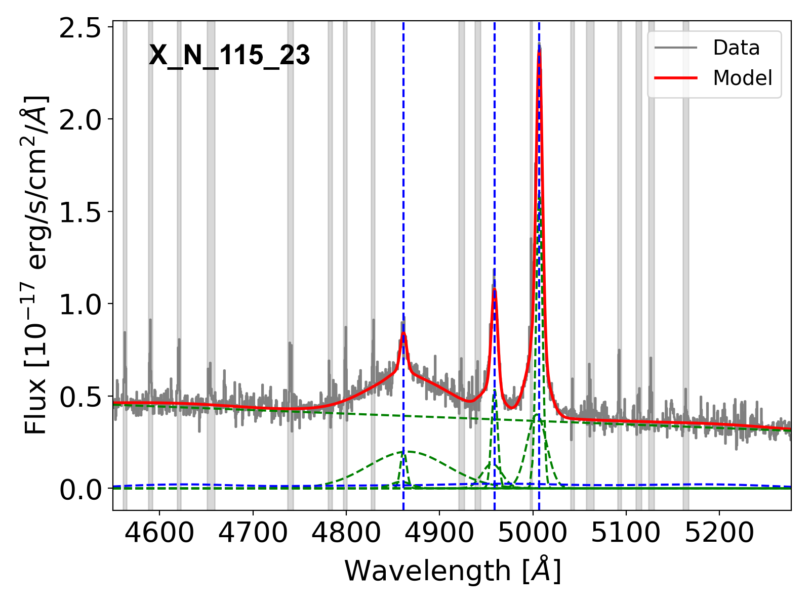
(a)

Figure 2: Integrated H-band spectrum of X_N_115_23 shown here as an example. The grey curve shows the observed spectrum, the red curve shows the reproduced overall emission line model, the blue dashed curve shows the iron emission and the dashed green curves show the continuum emission and the individual Gaussian components (Narrow, Broad and BLR) used to reproduce the profiles of various emission lines. The blue vertical lines indicate the location of $\mathrm{H\beta}\leavevmode\nobreak\$, [O iii] $\lambda$4959 and [O iii] $\lambda$5007. The vertical grey regions mark the channels with strong sky lines which were masked during the fitting procedure. The X-axis shows the rest frame wavelength after correcting for the redshift of the target and the Y-axis shows the observed flux density. The integrated spectra of the rest of the targets are shown in Appendix A.

5 Analysis and Results

The overall analysis of the reduced SINFONI cubes consists of three steps: (1) derive the properties of the ionized gas from modelling the integrated spectrum; (2) determine if the [O iii] emission is resolved after subtracting the AGN PSF and/or comparing the spatial profiles with a suitable PSF model; (3) measure the extension of the ionized gas at various velocity slices to determine the extent of the outflows. For the purpose of this paper, we focus the analysis only on the H-band SINFONI data to trace the kinematics of the ionized gas using the forbidden [O iii] transition. The results from the analysis of the K-band spectrum will be presented in a later publication.

5.1 Modelling the integrated spectrum

In this section, we describe the line fitting procedure on the integrated spectrum. While this paper will focus on the NLR properties, a more in-depth discussion on the BLR properties will be presented in a forthcoming publication (Vietri et al. in prep).

The integrated spectrum for each object was extracted from a circular aperture centered on the target which includes at least $\sim$95% of the total emission. The aperture used to extract the spectrum in each object is reported in Table 3. The target center was calculated using a two-dimensional Gaussian fit on the H-band continuum image obtained by collapsing the cube over all the spectral channels. The error on the spectrum was estimated creating an $rms$ spectrum obtained from an object-free region. The analysis of the H-band spectrum was restricted to the region spanned by $\mathrm{H\beta}\leavevmode\nobreak\$, [O iii] $\lambda$4959 and [O iii] $\lambda$5007. The residual sky lines were masked from the spectrum during the fitting procedure.

We modeled the extracted spectra using the scipy.curve-fit package in python, which uses the principle of least squares to find the optimal set of parameters for a given fitting model. We used a simple linear model to fit the AGN continuum. The iron emission was modeled using observed FeII templates from the literature (Boroson & Green, 1992; Véron-Cetty et al., 2004; Tsuzuki et al., 2006). The [O iii] and H$\beta$ emission lines were modeled with Gaussian functions and the kinematic components of the two lines were coupled with each other. The number of Gaussian components for the [O iii] emission line was restricted to two, and the addition of the second Gaussian depended on whether it minimizes the reduced chi-square value of the overall model. We will refer to these individual Gaussian components as “narrow” or “broad” according to the values of the line widths (FWHM), which are left as free parameters in the fitting procedure. We will not associate a physical meaning to each single Gaussian component, and consequently to the terms narrow and broad, but we will rather use a non-parametric approach in the paper to define velocity as described further down in this section. For $\mathrm{H\beta}\leavevmode\nobreak\$, a third Gaussian component or a broken power law was required to reproduce the Broad Line Region emission, which has been used to infer the black hole masses of the SUPER targets (more details in Vietri et al. (in prep)). The line centroid and width of the narrow and broad components of [O iii] $\lambda\lambda$4959,5007 and $\mathrm{H\beta}\leavevmode\nobreak\$ are tied to each other, based on the assumption of a common origin for these emission lines. Furthermore, the emission line ratio [O iii] $\lambda$5007:[O iii] $\lambda$4959 is set equal to $\sim$3:1 based on theoretical values (e.g. Storey & Zeippen, 2000; Dimitrijević et al., 2007). In order to estimate the uncertainty on the derived parameters, we created 100 mock spectra by adding $rms$ noise to the modeled spectrum and repeated the line fitting procedure on these mock spectra. The errors reported in Table 3 are the standard deviation for each parameter obtained with this procedure. Since we lack sufficient constraints to correct for dust reddening, we do not attempt to correct the emission line luminosities for extinction effects.

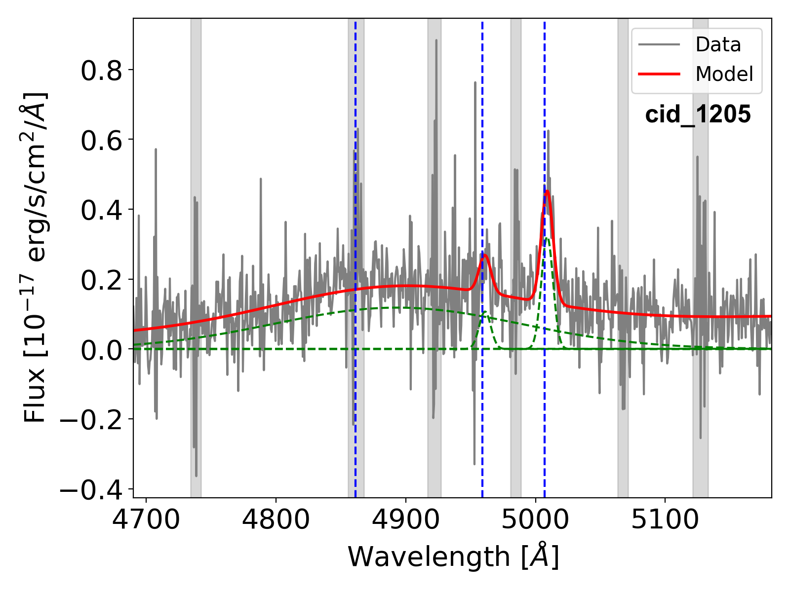
(a)

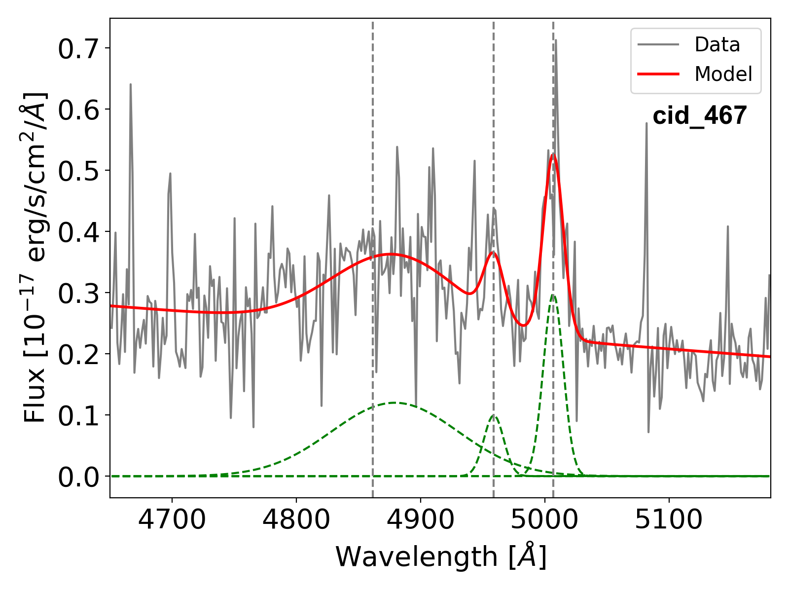
(b)

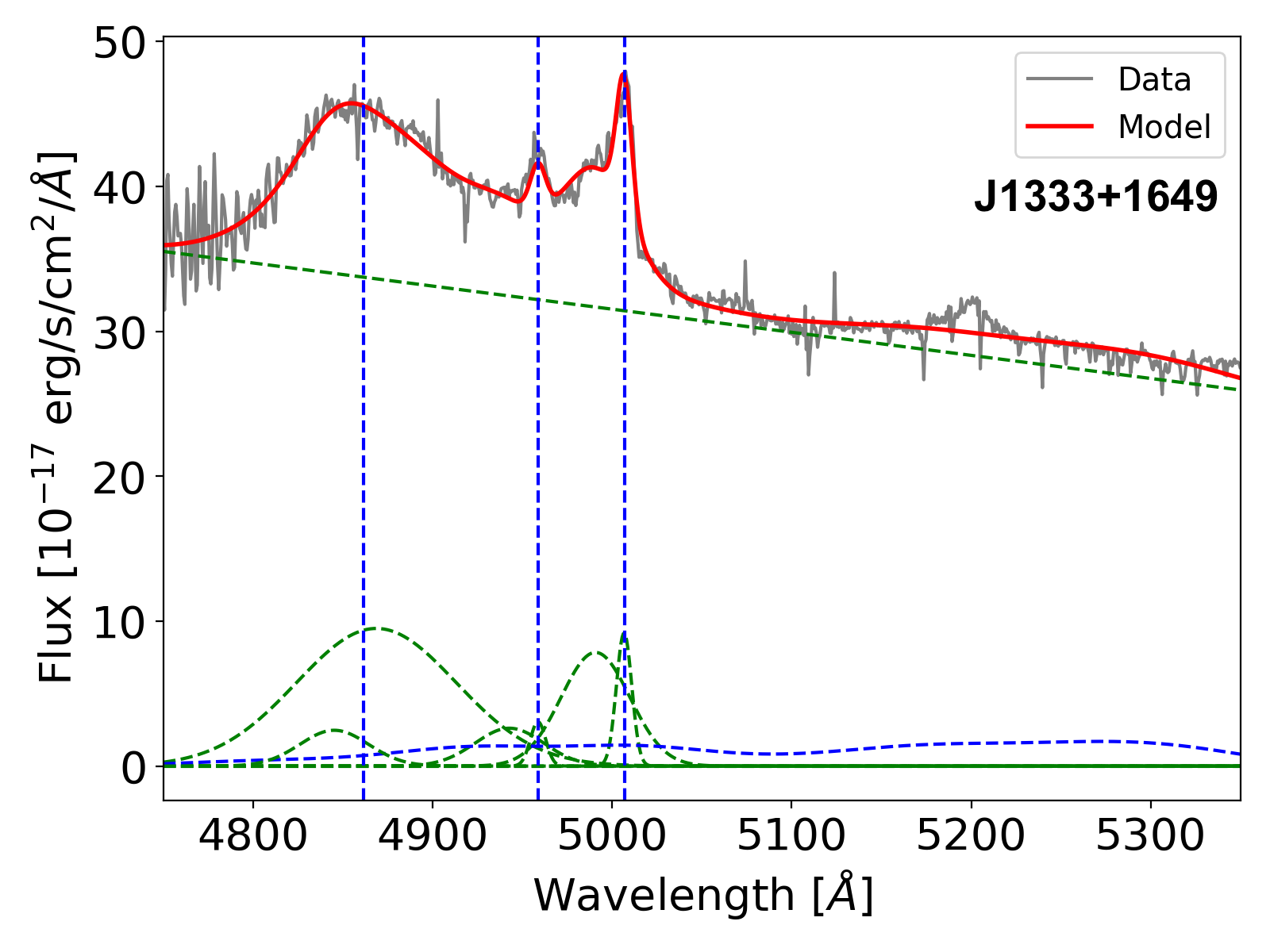
(c)

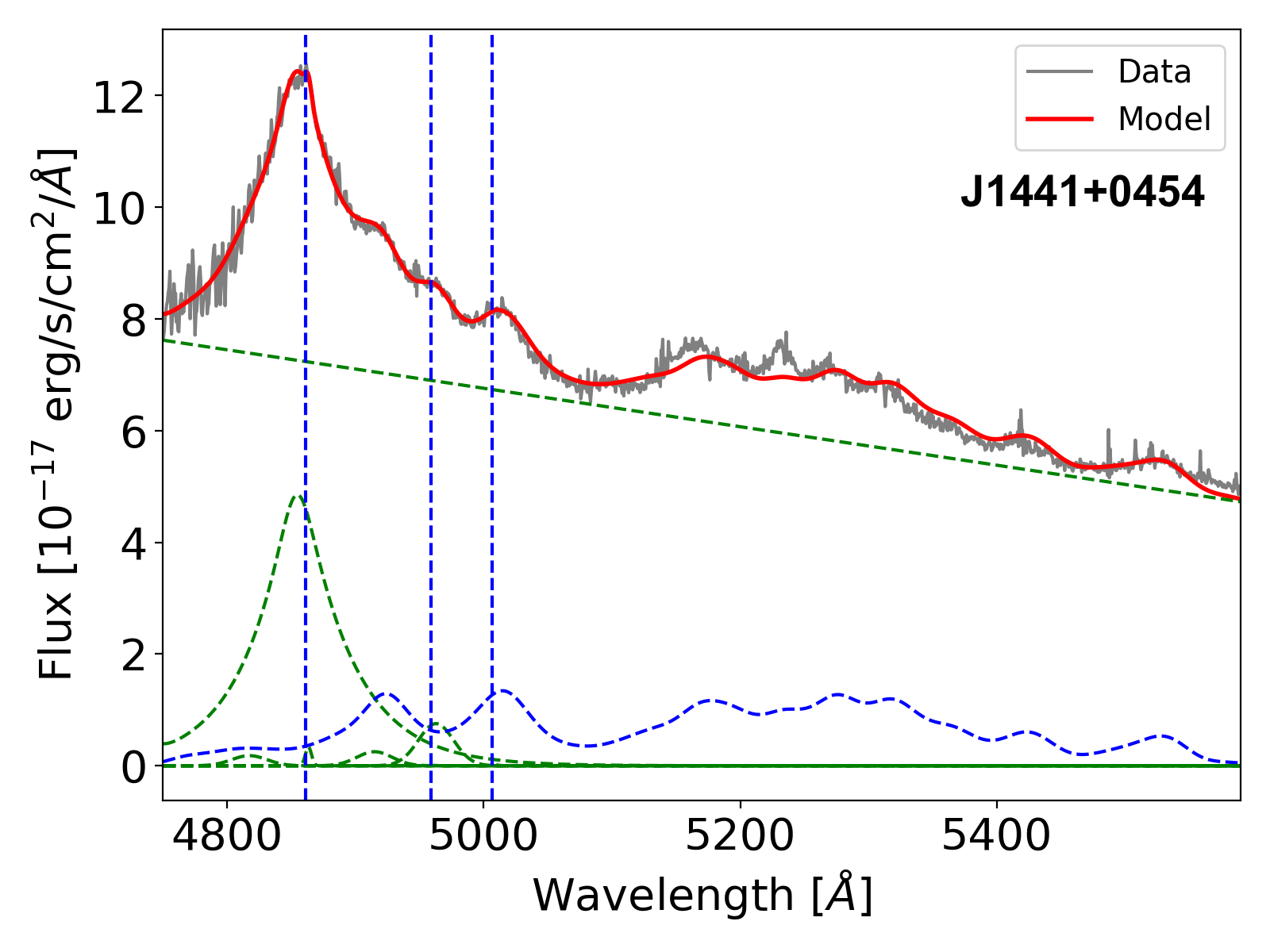
(d)

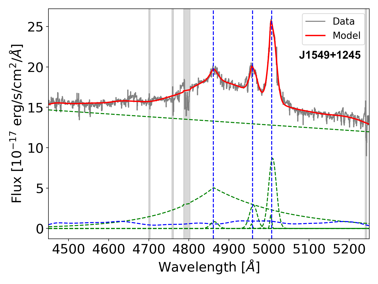
(e)

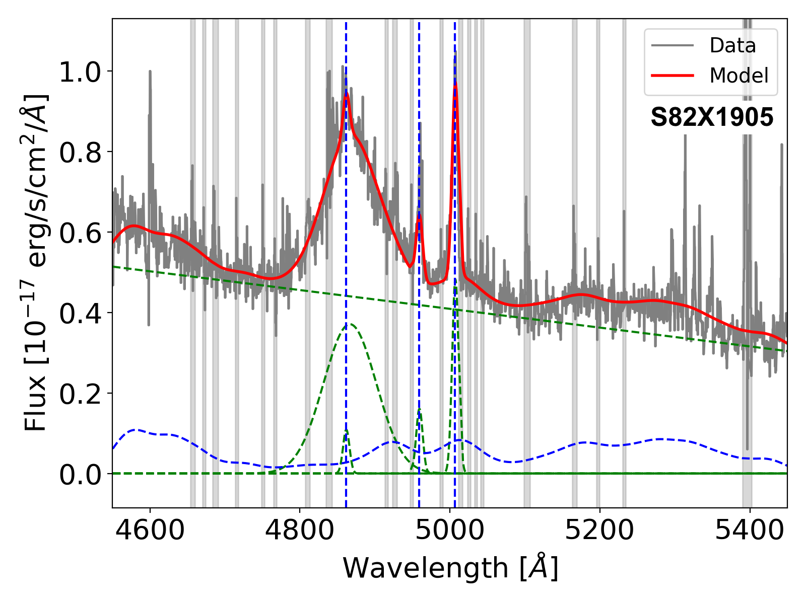
(f)

Figure 17: Same as Fig. 15 for cid_1205, cid_467, J1333+1649, J1441+0454, J1549+1245 and S82X1905.

As an example of the fit performed on the integrated H-band SINFONI spectra, we show the object X_N_115_23 along with the spectral model in Fig. 2. The integrated spectra for the rest of the Type-1 SUPER targets can be found in Appendix A. The line fitting parameters of the H-band spectrum are reported in Table 3. Out of the 21 Type-1 AGN presented in Table 2, we were able to derive line properties for 19 objects. X_N_53_3 is not detected in continuum and it does not show any emission lines in the H-band either. X_N_44_64 is detected in the continuum but does not have any emission lines. Finally, J1441+0454 is well detected in $\mathrm{H\beta}\leavevmode\nobreak\$, but the spectrum does not show the presence of [O iii] emission at the expected observed wavelength. This object is one of the brightest AGN in our sample and the possible lack of [O iii] emission at high bolometric luminosities has been previously reported in the literature (e.g. WISSH quasars: Bischetti et al., 2017). On the other hand, while the line fitting suggests that the spectrum around the expected location of [O iii] is dominated by strong iron emission, it also found a significant highly blue-shifted ($\sim$ -3000 km/s) [O iii] line with FWHM$\sim$1956 km/s. Such extreme blue-shift has also been observed before in the literature in high-redshift Extremely Red Quasars (ERQs, see Perrotta et al., 2019). Due to the degeneracy between the iron component and the [O iii] emission and the highly blended nature of the observed H$\beta$-[O iii] emission (see Fig. 17) we will limit the analysis of the [O iii] properties to the integrated spectum for this object and will not attempt to characterize the extended nature of the [O iii] emission in the next sections.

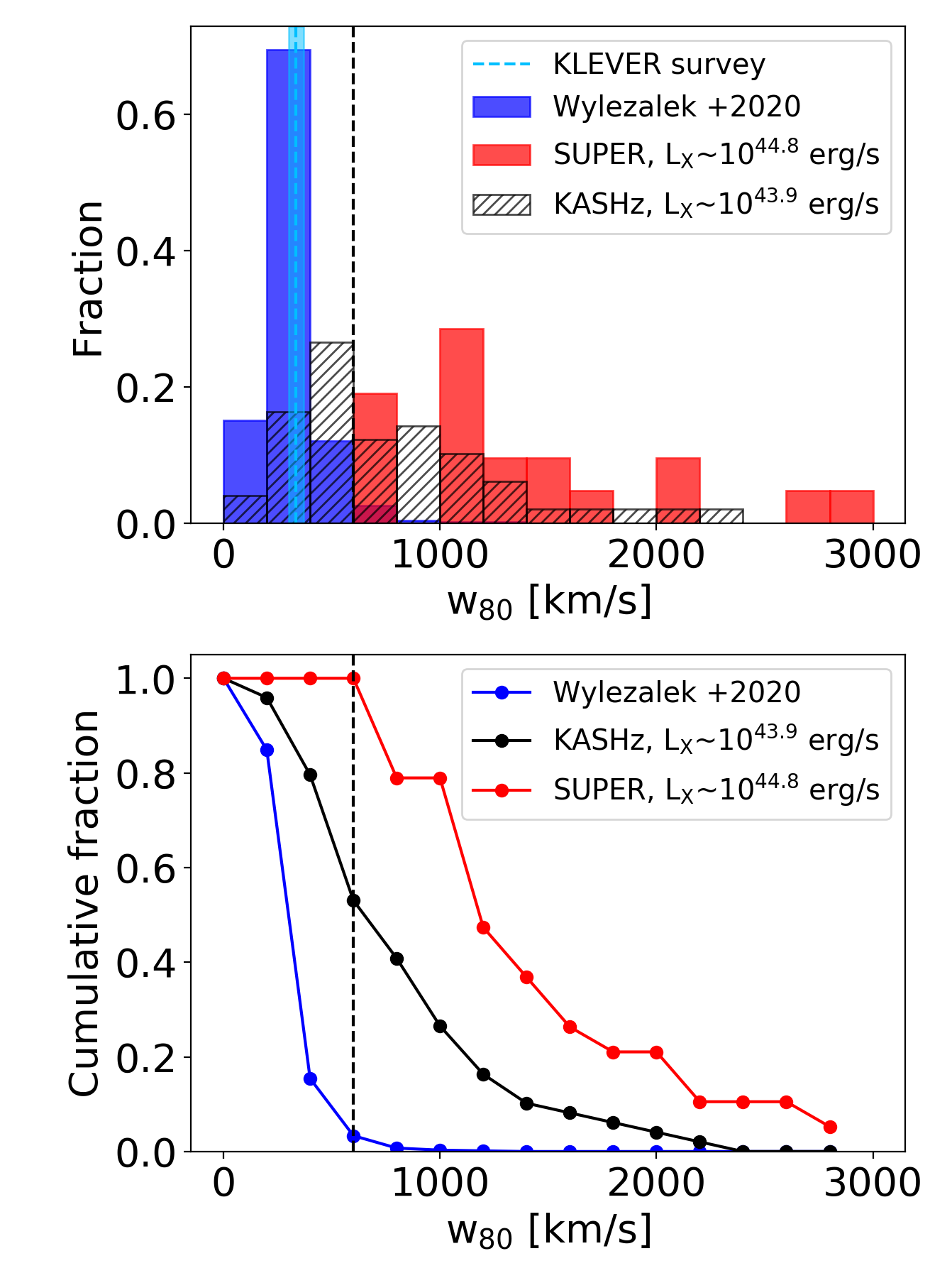
Figure 3: The top panel shows the distribution of the non-parametric velocity, $\mathrm{w_{80}}$ measured for [O iii] $\lambda$5007 line, for AGN and star forming samples from different surveys. The AGN sample consists of targets from the SUPER survey in red (this paper) and targets from KASHz survey matched in redshift in hatched black (Harrison et al., 2016). The Type-1 sample used in this paper has a median hard X-ray luminosity of 10^44.8 erg/s and the redshift-matched KASHz targets have a median X-ray luminosity of 10^43.9 erg/s. The blue histogram shows the $\mathrm{w_{80}}$ distribution of mass-matched low redshift star forming sample from Wylezalek et al. (2020), while the ocean-blue vertical bar shows the $\mathrm{w_{80}}$ value from the redshift and mass-matched star forming sample from the KLEVER survey (334$\pm$35 km/s, Curti et al. 2020). The dashed black-line at 600 km/s corresponds to the $\mathrm{w_{80}}$ value used in this work to define if a target hosts an AGN-driven outflow. The lower panel shows the inverse cumulative $\mathrm{w_{80}}$ distribution with the same color coding as in the top panel. It is clear from both the panels that targets from the SUPER survey occupy the higher end of the $\mathrm{w_{80}}$ distribution. Based on the $\mathrm{w_{80}}$ criteria, all the targets in the SUPER survey show the presence of outflows, and $\sim$52% of the redshift matched targets in the KASHz survey show outflows.

Table 3: Narrow Line Region properties from the line fitting of the integrated H-band SINFONI spectra of the SUPER sample.

Target	$\mathrm{\lambda_{range}^{a}}$	$D_{ext}^{b}$	$\mathrm{z_{[{O\textsc{iii}}]\leavevmode\nobreak\ }^{c}}$	log L${}_{[{O\textsc{iii}}]\leavevmode\nobreak\ }^{d}$		$\mathrm{v_{[{O\textsc{iii}}]\leavevmode\nobreak\ }^{e}}$					log L${}_{H\beta}^{d}$
				narrow	broad	FWHMnarrow	FWHMbroad	$\mathrm{v_{10}}$	$\mathrm{w_{80}}$	$\mathrm{v_{max}}$	narrow	broad
	Å	arcsec		erg/s	erg/s	km/s	km/s	km/s	km/s	km/s	erg/s	erg/s
X_N_160_22	4550–5200	1.0	2.442	43.11$\pm$0.04	43.30$\pm$0.07	869$\pm$50	3035$\pm$185	-2333$\pm$146	2816$\pm$160	3637$\pm$222	42.60$\pm$0.08	–
X_N_81_44	4500–5420	0.9	2.317	42.68$\pm$0.04	42.19$\pm$0.13	494$\pm$30	1851$\pm$130	-336$\pm$40	775$\pm$108	1682$\pm$117	41.43$\pm$0.05	43.24$\pm$0.05
X_N_66_23	4600–5250	0.7	2.384	–	43.16$\pm$0.03	–	900$\pm$44	-495$\pm$36	1001$\pm$51	764$\pm$38	42.84$\pm$0.05	–
X_N_35_20	4600–5200	0.3	2.260	–	41.87$\pm$0.45	–	643$\pm$106	-330$\pm$78	681$\pm$209	546$\pm$90	–	–
X_N_12_26	4450–5180	0.8	2.471	–	42.41$\pm$0.07	–	933$\pm$184	-680$\pm$57	1044$\pm$89	792$\pm$156	–	42.06$\pm$0.07
X_N_4_48	4500–5250	0.5	2.314	–	42.24$\pm$0.07	–	1126$\pm$151	-648$\pm$84	1198$\pm$100	956$\pm$129	–	41.50$\pm$0.06
X_N_102_35	4620–5400	0.3	2.190	42.51$\pm$0.13	42.76$\pm$0.13	550$\pm$112	1473$\pm$261	-1076$\pm$140	1501$\pm$170	1761$\pm$295	41.18$\pm$0.10	42.14$\pm$0.09
X_N_115_23	4550–5280	0.7	2.340	43.27$\pm$0.03	43.18$\pm$0.02	471$\pm$24	1495$\pm$62	-623$\pm$57	1015$\pm$67	1437$\pm$56	42.38$\pm$0.06	42.13$\pm$0.28
cid_166	4430–5185	0.6	2.460	42.60$\pm$0.11	43.17$\pm$0.07	503$\pm$91	1703$\pm$150	-1502$\pm$41	1755$\pm$109	2136$\pm$155	41.77$\pm$0.04	42.89$\pm$0.10
cid_1605	4650–5200	0.4	2.117	–	42.43$\pm$0.43	–	1095$\pm$244	-573$\pm$98	1153$\pm$142	929$\pm$208	–	–
cid_346	4550–5450	0.7	2.216	–	42.97$\pm$0.04	–	1989$\pm$212	-1343$\pm$166	2142$\pm$231	1689$\pm$181	–	42.74$\pm$0.14
cid_1205	4700–5200	0.3	2.256	–	42.66$\pm$0.04	–	636$\pm$72	-223$\pm$36	717$\pm$48	540$\pm$61	–	–
cid_467	4600–5200	0.4	2.284	–	42.87$\pm$0.43	–	1256$\pm$132	-702$\pm$112	1368$\pm$154	1067$\pm$112	–	–
J1333+1649	4750–5350	1.1	2.098	44.00$\pm$0.02	44.58$\pm$0.04	602$\pm$22	2700$\pm$80	-2271$\pm$78	2714$\pm$96	3248$\pm$87	–	44.08$\pm$0.12
J1441+0454*	4730–5350	1.0	2.053	–	43.41$\pm$0.03	–	1956$\pm$96	-3698$\pm$70	2161$\pm$102	1661$\pm$82	42.29$\pm$0.13	42.79$\pm$0.19
J1549+1245	4450–5250	1.0	2.367	43.15$\pm$0.10	44.49$\pm$0.05	327$\pm$49	1362$\pm$25	-613$\pm$27	1457$\pm$38	1413$\pm$32	41.40$\pm$0.10	43.47$\pm$0.06
S82X1905	4550–5450	0.8	2.272	–	42.82$\pm$0.04	–	607$\pm$59	-304$\pm$34	678$\pm$55	515$\pm$54	42.18$\pm$0.15	–
S82X1940	4550–5400	0.6	2.349	42.28$\pm$0.03	42.54$\pm$0.03	354$\pm$20	1336$\pm$71	-820$\pm$51	1186$\pm$39	1373$\pm$71	41.30$\pm$0.17	42.09$\pm$0.09
S82X2058	4600–5400	0.6	2.314	42.44$\pm$0.08	42.61$\pm$0.08	539$\pm$61	1442$\pm$109	-972$\pm$88	1340$\pm$95	1701$\pm$234	42.01$\pm$0.09	41.67$\pm$0.40

Notes:
^aThe wavelength range used for the emission line fitting.
^bThe diameter (in arcsec) of the circular aperture centered on the target used to extract the spectrum.
^cRedshift of the target determined from the peak location of the [O iii] $\lambda$5007 in the integrated spectrum.
^dThe luminosity of the individual Gaussian components in erg/s, not corrected for reddening. The emission lines were modeled using multiple Gaussian components and the terms “narrow” and “broad” refer to these individual Gaussian components parameters. In case of single Gaussian fits, the Gaussian component is classified as broad if the width (FWHM) ¿ 600 km/s.“–” means that there was no detection of the corresponding component. The errors indicate 1$\sigma$ uncertainty.
^eLine widths (FWHM) of the individual Gaussian components. $\mathrm{v_{10}}$ and $\mathrm{w_{80}}$ are the non-parametric velocities and $\mathrm{v_{max}}$ the maximum velocity as defined in Sect. 5.1.
*The fit does not constrain the NLR properties due to contamination from telluric absorption and strong contribution from FeII emission. The reported [O iii] emission is highly blue-shifted ($\sim$-3000 km/s) and the [O iii] redshift corresponds to this component.
There is no detection of lines in X_N_53_3 and X_N_44_64.

We adopt non-parametric measures for the line properties, which has the advantage that the parameter values do not depend on the fitting function adopted (e.g. the number of Gaussian components) that may strongly depend on the signal-to-noise of the spectrum under investigation (see e.g. Zakamska & Greene 2014, Harrison et al. 2014 for more details). In particular, we measure the velocity at the 10th percentile of the overall [O iii] line profile ($\mathrm{v_{10}}$) and the velocity width of the line that contains 80$\%$ of the line flux ($\mathrm{w_{80}=v_{90}-v_{10}}$). For a Gaussian profile, the value of $\mathrm{w_{80}}$ approximately corresponds to the FWHM of the emission line. We also compute the maximum velocity, $\mathrm{v_{max}}$, following the definition by Rupke & Veilleux (2013) as the shift between the narrow and the broad Gaussian components of [O iii] plus twice the sigma of the broad Gaussian. For fits with single Gaussian, we estimate $\mathrm{v_{max}}$ as twice the sigma of the broad Gaussian. The non-parametric measures of velocities and the line widths are reported in Table 3.

In the following, we will use $\mathrm{w_{80}}$ to identify AGN with clear signatures of outflows. Fig. 3 shows the distribution of $\mathrm{w_{80}}$ for the AGN sample from SUPER and KASHz surveys in red and black histograms respectively. The KASHz sample is matched in redshift (z$\sim$2.0–2.5) to the SUPER sample. For comparison, we also plot the $\mathrm{w_{80}}$ distribution of low-redshift mass-matched sample of MANGA galaxies from Wylezalek et al. (2020), which is shown in blue in Fig. 3. The light blue vertical area denotes the $\mathrm{w_{80}}$ value from a stacked spectrum of mass-matched and redshift-matched galaxies from the KLEVER survey (Curti et al., 2020), a high redshift survey targeting star forming galaxies. The stellar mass of the overall SUPER sample has been used to mass-match the comparison samples, as most of the Type-1 AGN do not have reliable stellar mass measurements (Circosta et al., 2018).

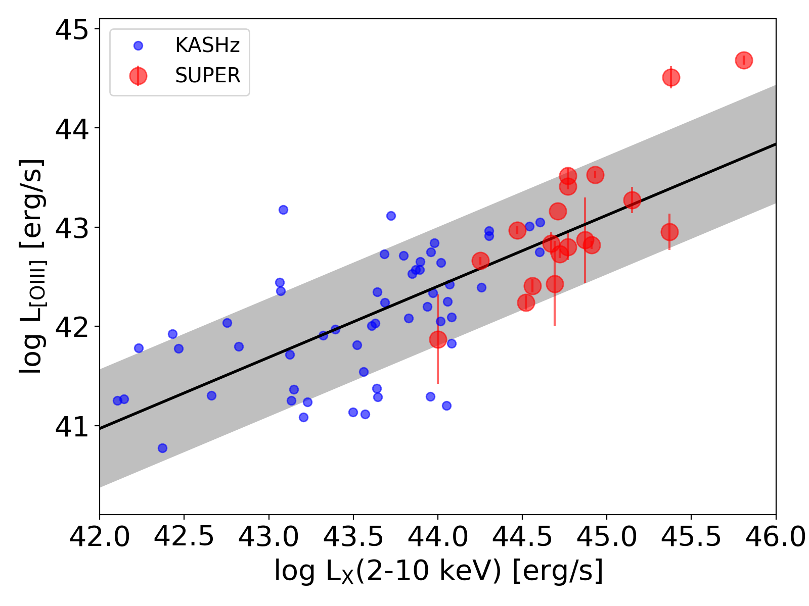
Figure 4: Total [O iii] luminosity vs. hard X-ray luminosity ($\mathrm{L_{X}}$(2-10 keV) for the SUPER (red circles) and KASHz targets (blue data points), the latter from a similar survey targeting X-ray selected AGN at high redshift. The combined dataset of KASHz and SUPER show a positive correlation between the two quantities, shown by the black line. The shaded region represents the 1$\sigma$ scatter on the relation. KASHz targets occupy the lower X-ray luminosity range compared to SUPER targets, which may explain the difference in the distribution of $\mathrm{w_{80}}$ in the two surveys in Fig. 3.

From the histogram and the cumulative distributions in Fig. 3, it is clear that the AGN sample from the KASHz and SUPER surveys occupy the higher end of $\mathrm{w_{80}}$ values compared to mass-matched samples at low as well as high redshift star forming galaxies. A $\mathrm{w_{80}}$ value of 600 km/s lies at the high end of the tail of the $\mathrm{w_{80}}$ distribution for low-redshift star forming galaxies and it is well above the average values obtained from KLEVER. Consequentely, we will consider in this paper a $\mathrm{w_{80}}$ value greater than 600 km/s as a signature of an AGN-driven outflow. We note that similar cut in $\mathrm{w_{80}}$ was also used in previous works (e.g. Harrison et al., 2016) and is a conservative estimate when compared to the cuts used in other works (e.g. 500 km/s in Wylezalek et al., 2020).

Based on the above definition of outflows, all the observed Type-1 AGN from SUPER detected in [O iii] show the presence of AGN-driven outflows (90% outflow detection rate if we include targets which were observed and not detected in [O iii] ). The KASHz survey, on the other hand, reported $\sim$50% of their sample having $\mathrm{w_{80}}$ larger than 600 km/s (Harrison et al., 2016), therefore a lower fraction of AGN with clear outflow signatures according to the adopted definition. If we restrict the KASHz sample to the same redshift range of SUPER, $2<z<2.5$, the fraction of KASHz targets hosting outflows results to be at $\sim 52\%$ as shown in Fig. 3.The difference between the $\mathrm{w_{80}}$ distributions for SUPER and KASHz surveys is probably due to the different luminosity range of the AGN sampled by these surveys. Fig. 4 shows the relation between total [O iii] luminosity and hard X-ray luminosity for the targets presented in this paper as well as for the redshift-matched AGN sample from the KASHz survey. We have eight objects in common between the two surveys (for both Type-1 and Type-2 targets) and the $\mathrm{w_{80}}$ values derived from SINFONI and KMOS for these objects are perfectly consistent with each other. As it can be clearly seen from this figure, there is little overlap between the luminosity ranges covered by the two surveys: $\approx 90\%$ of the Type-1 sample presented in this paper has L${}_{\rm[2-10kev]}>3\times 10^{44}$ erg s^-1, while $\approx 90\%$ of the KASHz AGN are at L${}_{\rm[2-10kev]}<3\times 10^{44}$ erg s^-1 (Fig. 3, blue data points). As already reported in previous works (e.g. Fiore et al., 2017) and presented for the SUPER Type-1 sample in sect. 6, there is a positive correlation between the velocity associated with the outflow and the bolometric luminosity of the AGN. Therefore, the detection of a higher fraction of outflows in the SUPER sample compared to the KASHz survey could naturally be explained with the prevalence of the faster outflows at higher bolometric luminosity (see Fig. 3).

Although we will use non-parametric measures along the paper to characterize the line properties, we also report here the incidence of outflows in our sample based on the presence of a broad Gaussian component in the line fit. For the 21 Type-1 AGN presented in this paper, 14 targets require a broad component with width $\sim$1000-3000 km/s in their [O iii] profile. We can therefore claim based on this measure that $67\%$ ($\sim 75\%$ if we limit to the objects with detected [O iii] ) of the SUPER Type-1 sample have fast ionized outflows. This outflow incidence fraction is much higher than some previous works for star forming as well as AGN host galaxies (e.g. Harrison et al., 2016; Förster Schreiber et al., 2018; Swinbank et al., 2019) and comparable to other lower redshift studies targeting AGN (e.g. Rakshit & Woo, 2018; Davies et al., 2020a). As we mentioned earlier, this method of classification for outflows is highly dependent on the signal-to-noise of the spectra and models used for line fitting, and therefore these comparisons are subject to biases.

Apart from the detection of the bright emission lines already discussed in this section, we also detect $\mathrm{H\beta}\leavevmode\nobreak\$ in all Type-1 sources, except cid_1205 which shows a strong skyline at the location of $\mathrm{H\beta}\leavevmode\nobreak\$ emission. All targets but X_N_66_23 show the detection of a BLR $\mathrm{H\beta}\leavevmode\nobreak\$ component. The non-detection of the BLR component of H$\beta$ in X_N_66_23 is possibly a consequence of the short exposure time leading to a low S/N in the spectrum. Compared to the [O iii] profile where the broad component was detected in $\sim$75% of the sample, 62% of the sample required an additional broad Gaussian component for $\mathrm{H\beta}\leavevmode\nobreak\$ line. The $\mathrm{H\beta}\leavevmode\nobreak\$ component flux is usually 10 times fainter than that of [O iii] line in Type-1 AGN (e.g. Leighly, 1999; Rodríguez-Ardila et al., 2000), hence for the current sample the non-detection of broad $\mathrm{H\beta}\leavevmode\nobreak\$ could be simply due to the lower S/N. Although the kinematic components of the [O iii] and the $\mathrm{H\beta}\leavevmode\nobreak\$ line are coupled to each other, the relatively low S/N of the $\mathrm{H\beta}\leavevmode\nobreak\$ line means that the addition of second Gaussian in $\mathrm{H\beta}\leavevmode\nobreak\$ profile does not change the $\chi^{2}$ of the fit in some targets. Based on this consideration, we will use the results on the [O iii] line profile to assess the incidence of AGN-driven outflows in our sample. We refer the reader to Vietri et al. (2020) for further discussion on $\mathrm{H\beta}\leavevmode\nobreak\$ line profile.

5.2 Extension of the [O iii] emission line region

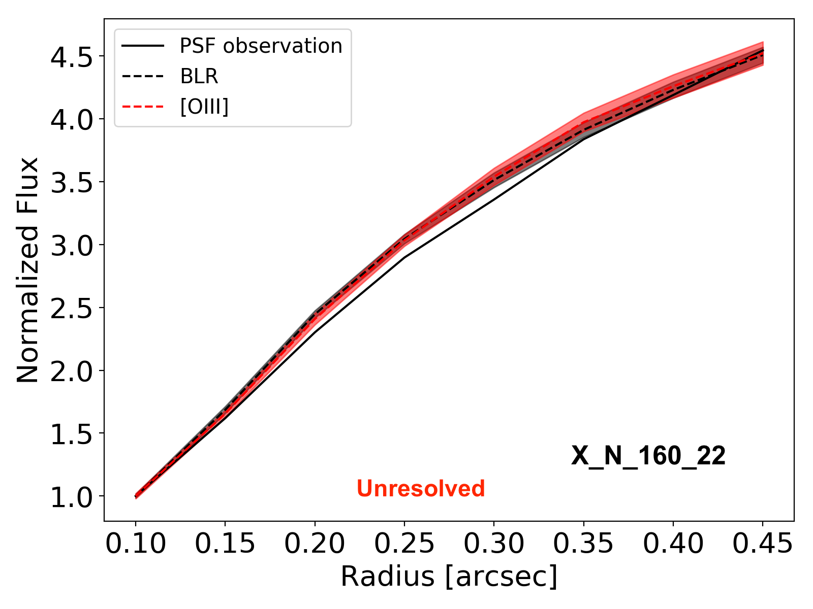
(a)

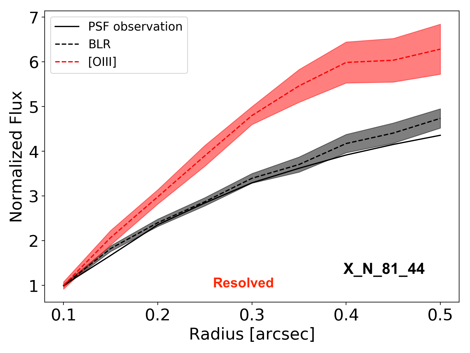
(b)

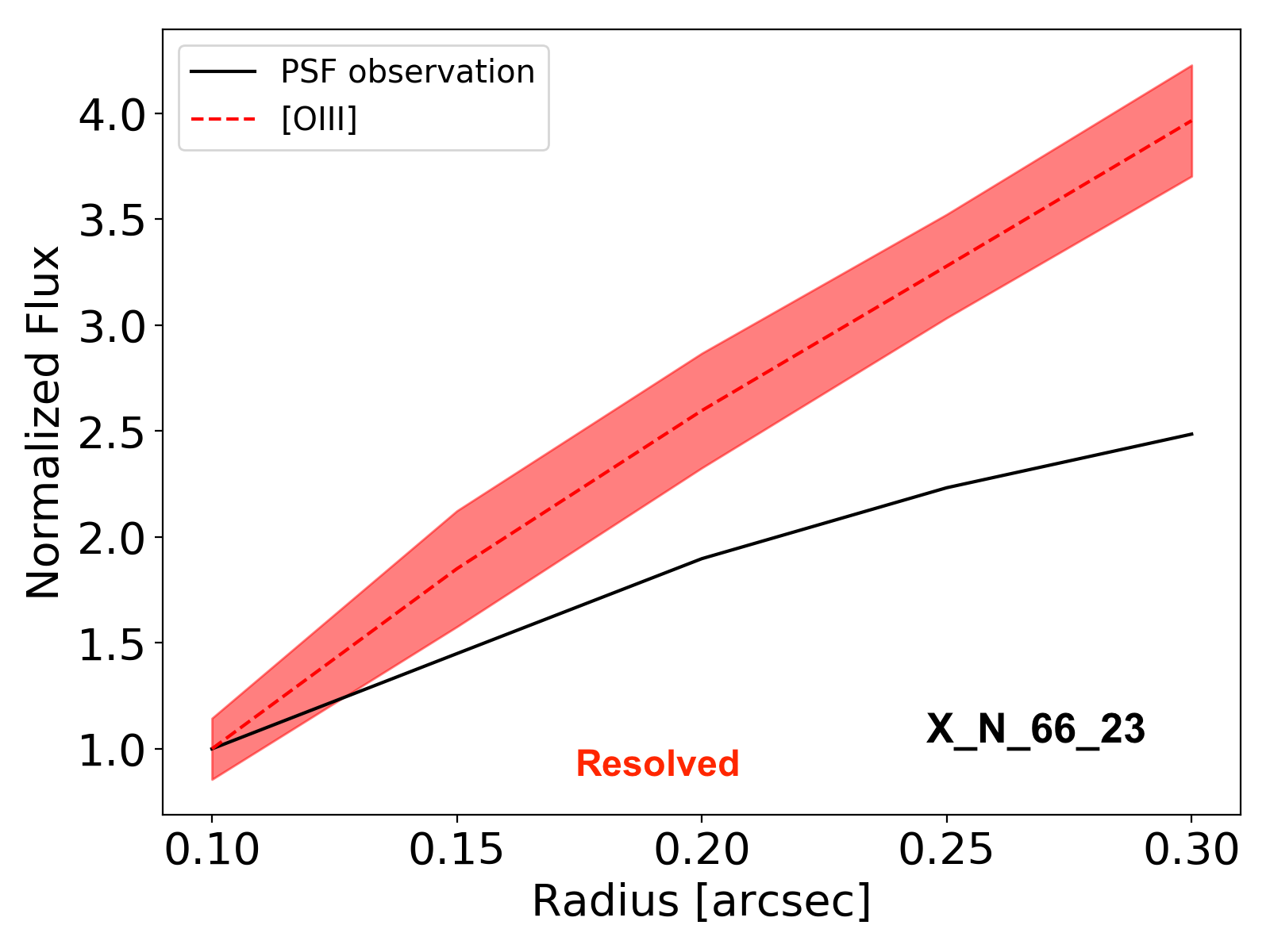
(c)

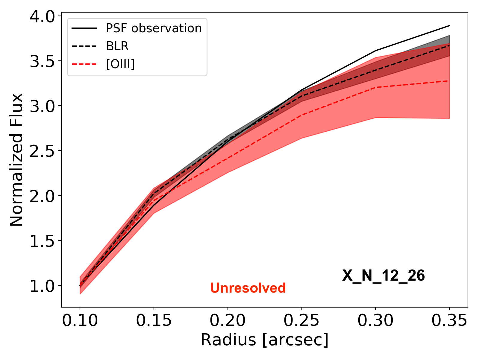
(d)

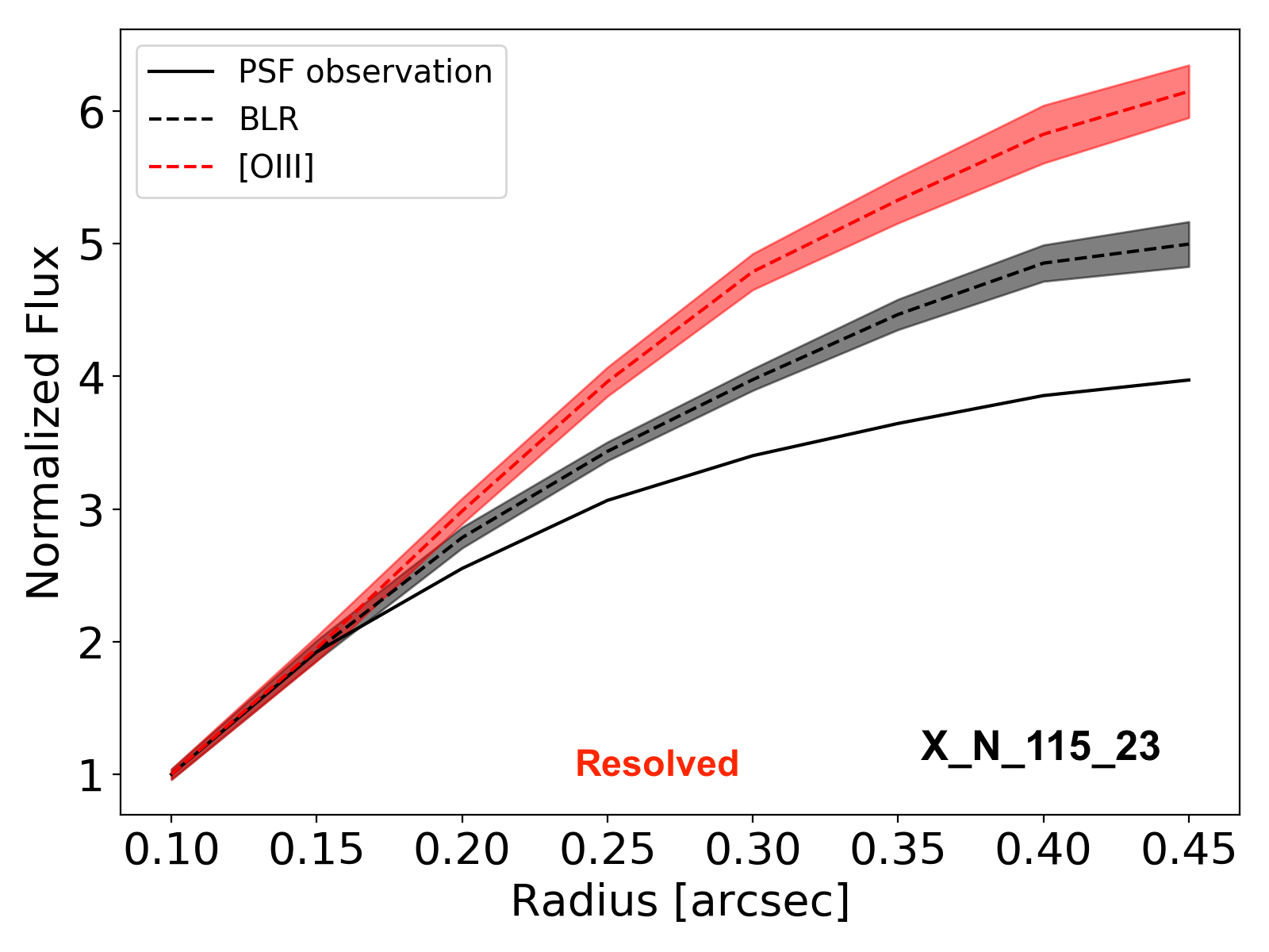
(e)

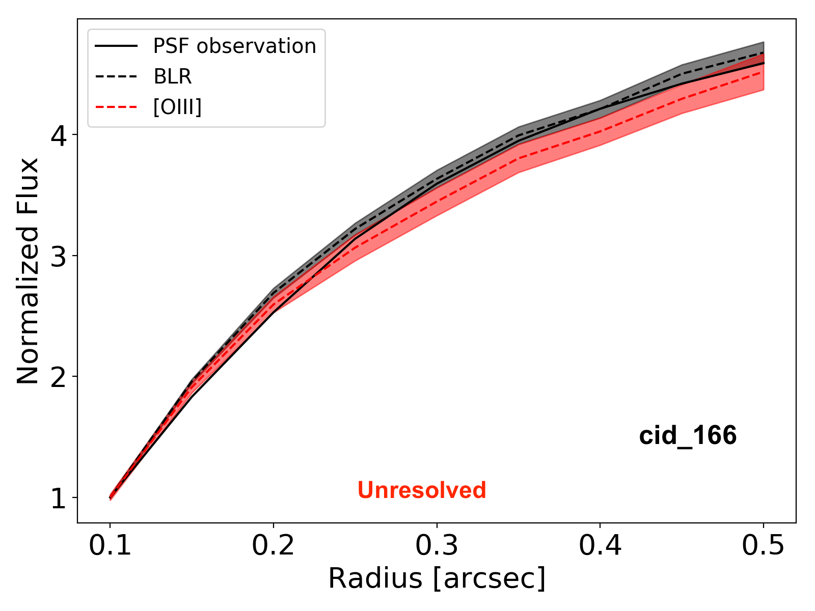
(f)

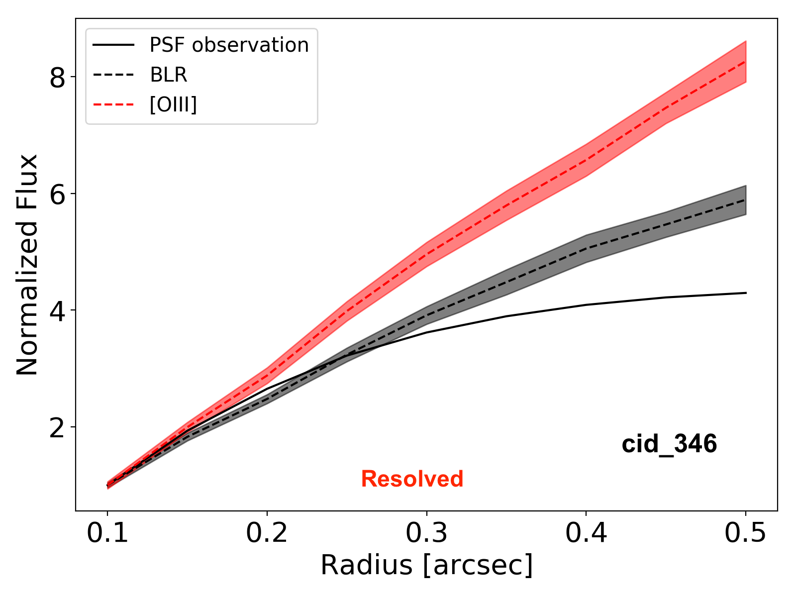
(g)

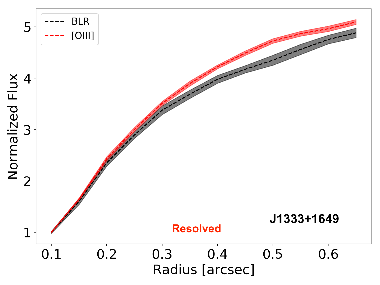
(h)

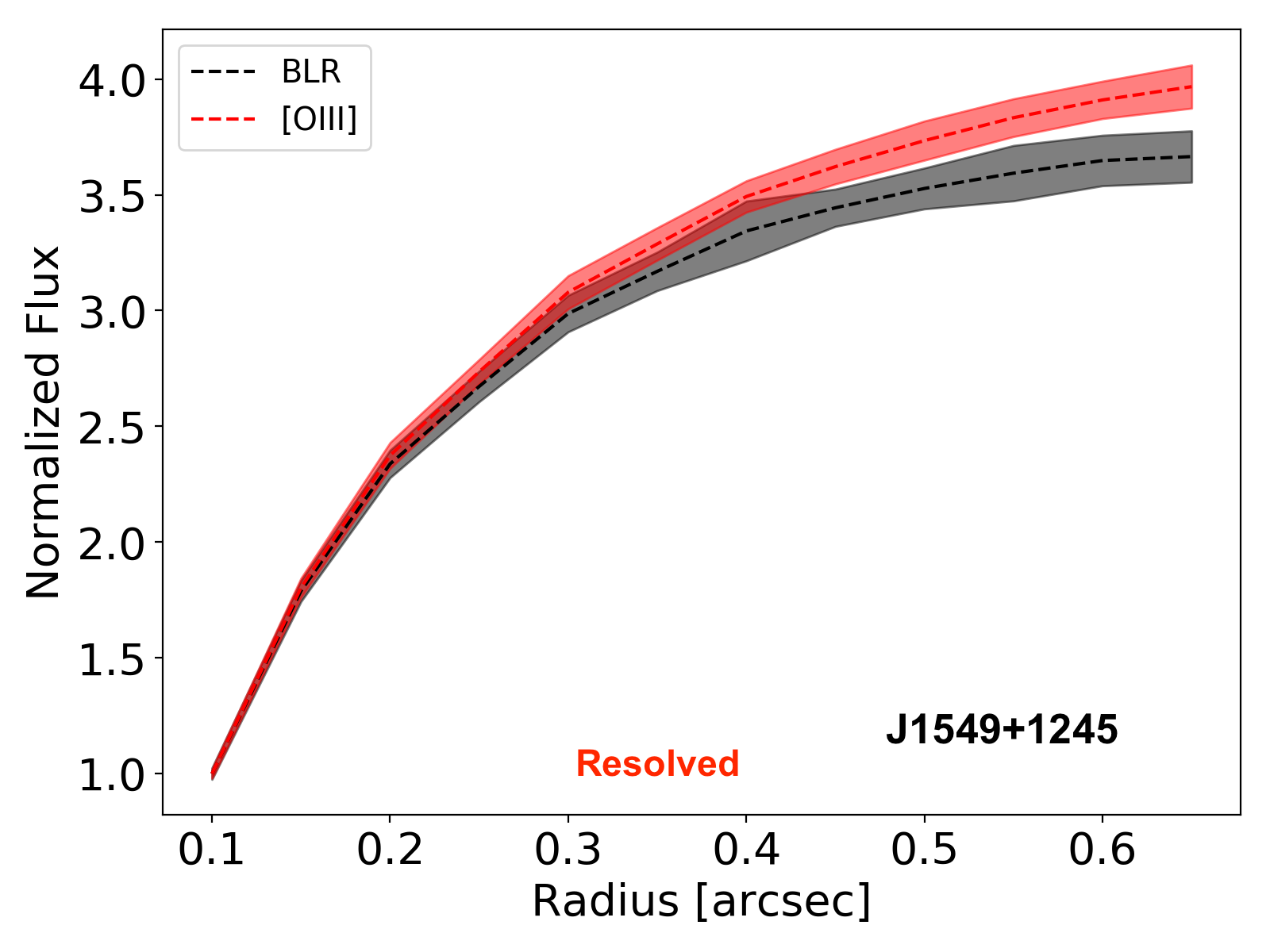
(i)

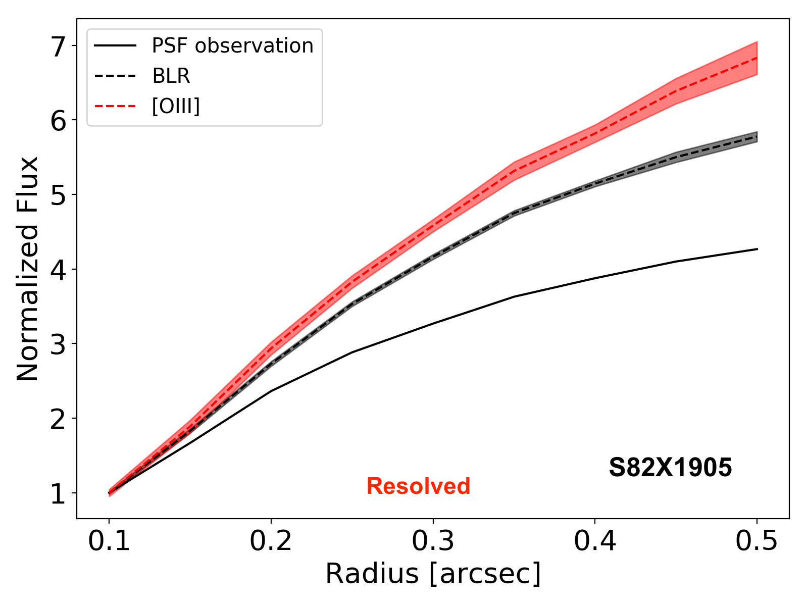
(j)

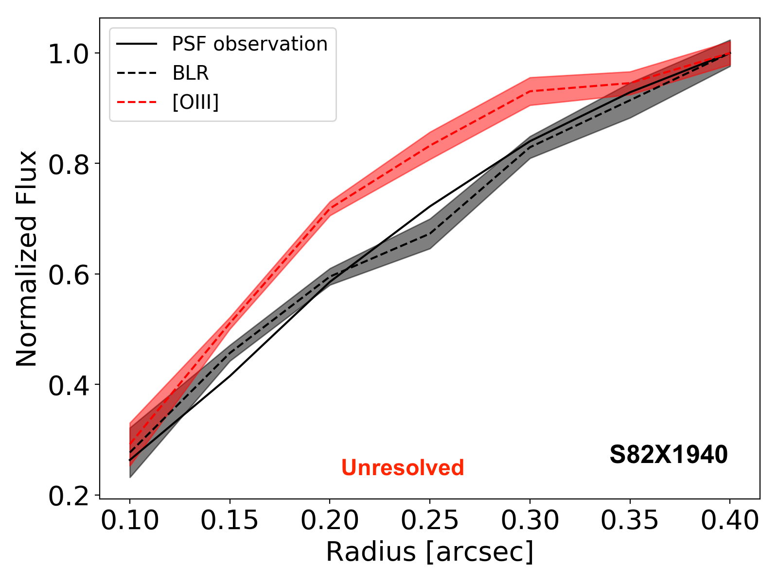
(k)

Figure 5: Curves-of-growth for the Type-1 sample as described in section 5. The solid black line shows the curve from the image obtained by collapsing the PSF-observation cube at the location of [O iii] $\lambda$5007 channels. The $\mathrm{H\beta}\leavevmode\nobreak\$ BLR component is shown as a dashed black curve with the grey area showing the 1$\sigma$ uncertainly. The BLR component is unresolved and serves as a proxy to determine the PSF during the observations which is also compared with the dedicated PSF star observation. The red curve shows the curve-of-growth for the total [O iii] emission i.e. narrow and broad components. All the uncertainty are at 1$\sigma$ levels. The BLR component is not plotted for X_N_66_23 as it remains undetected. For the rest of the Type 1 sample in the SUPER survey, the S/N is not enough to perform such a curve-of-growth analysis.

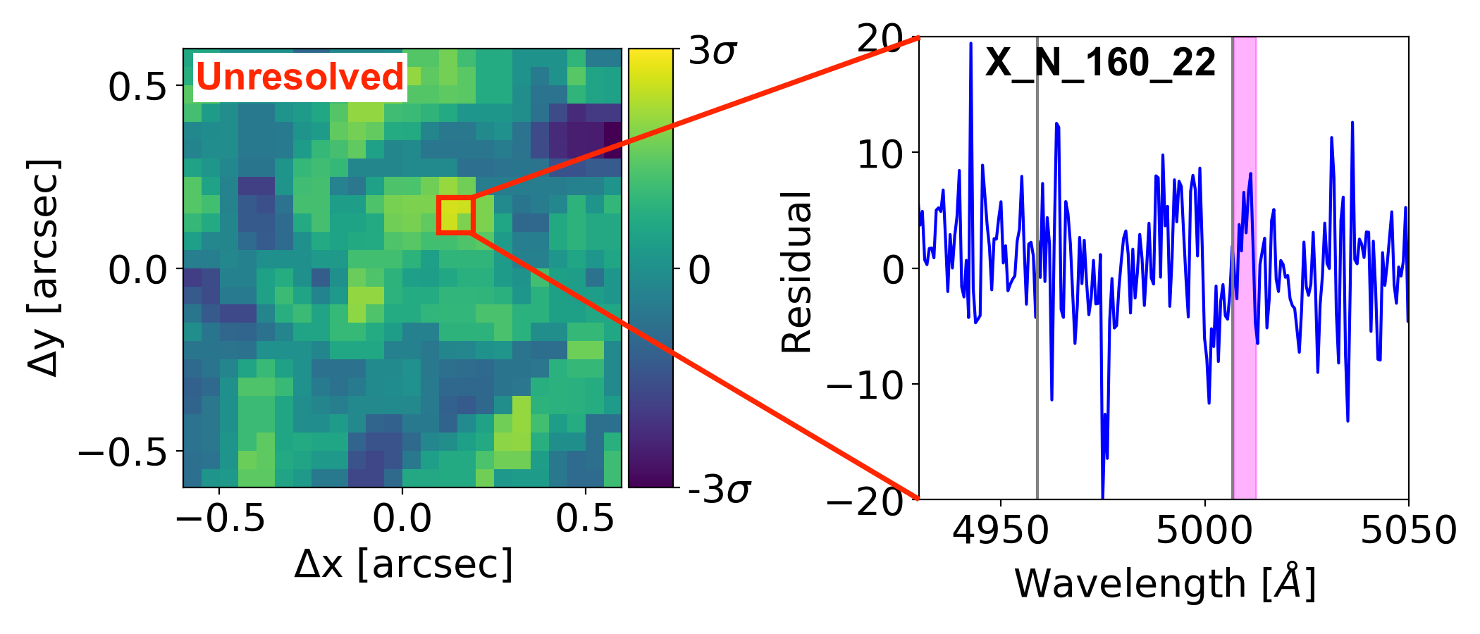
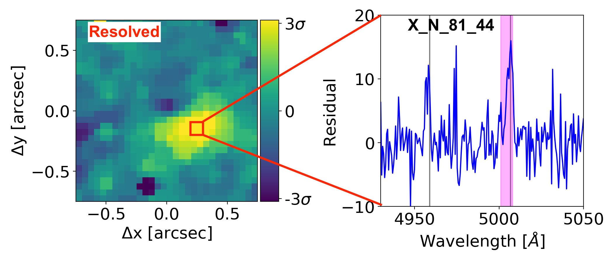
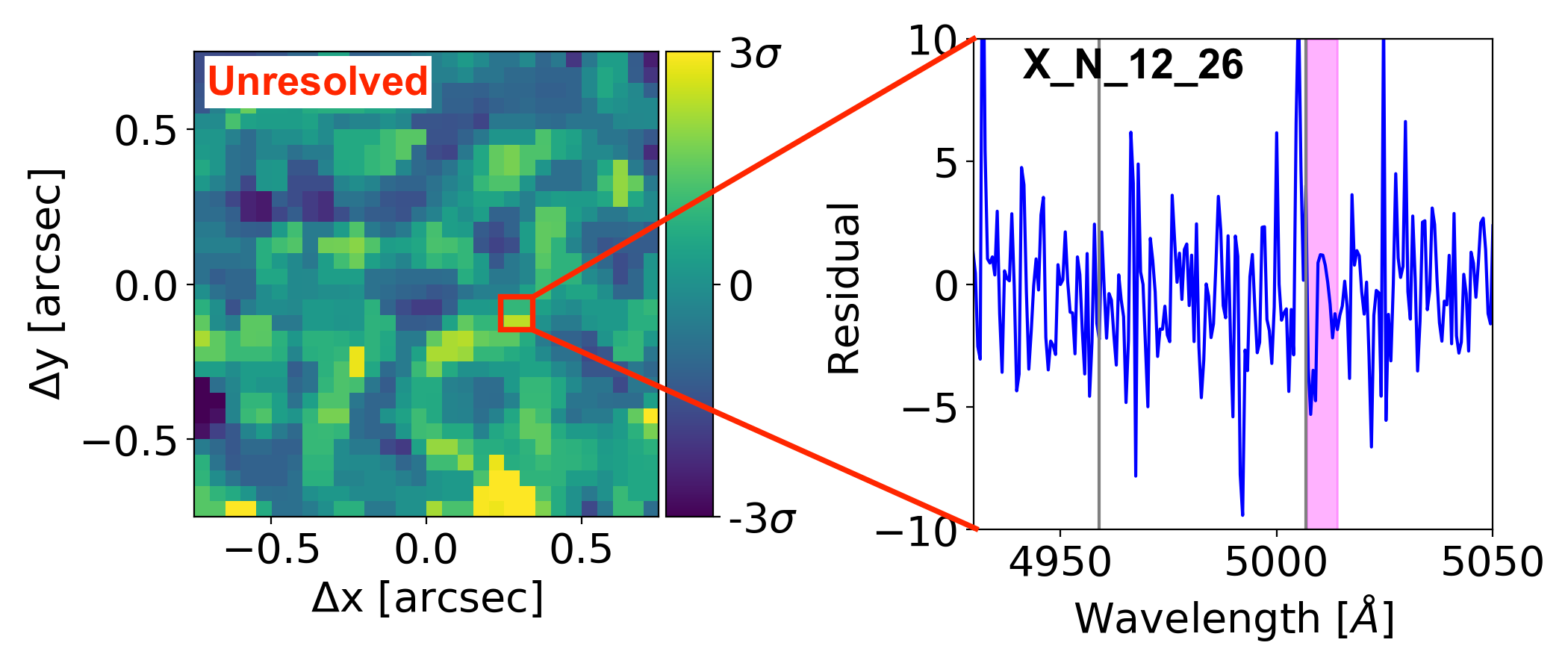
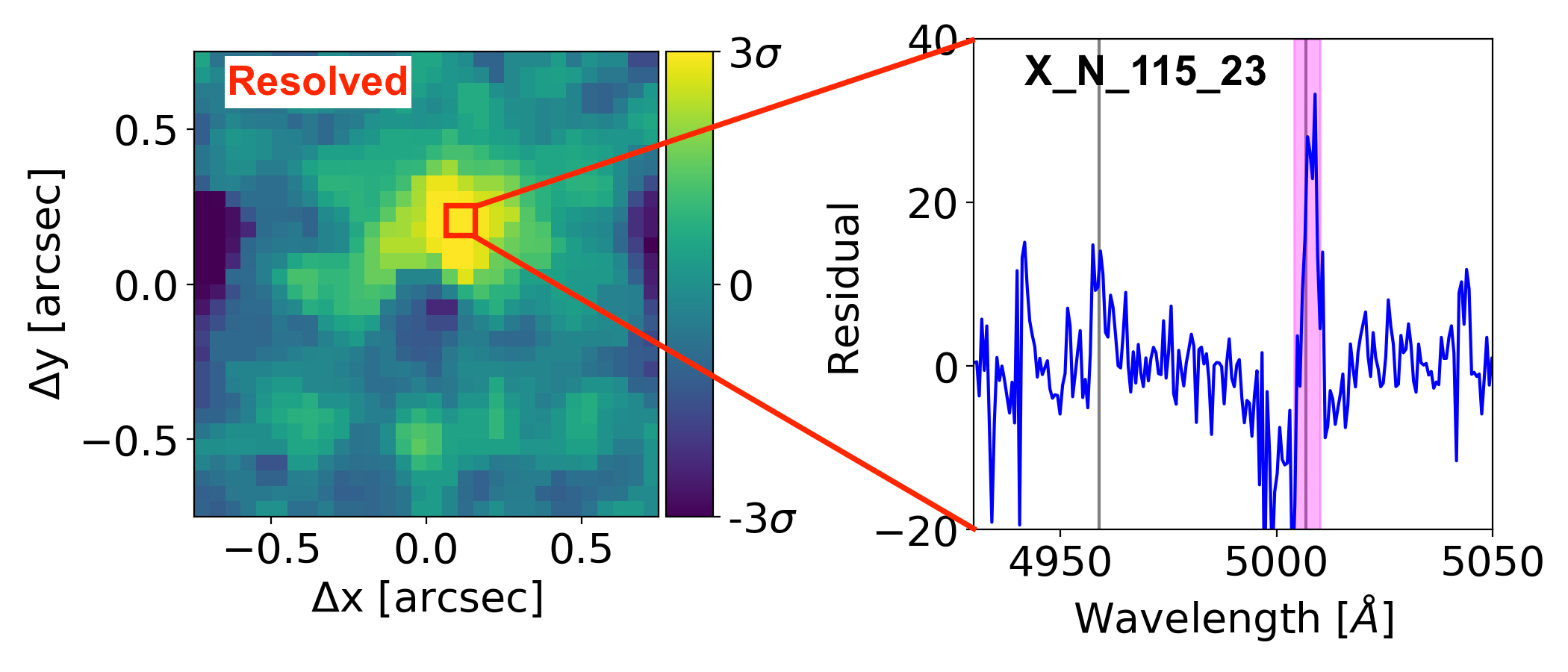
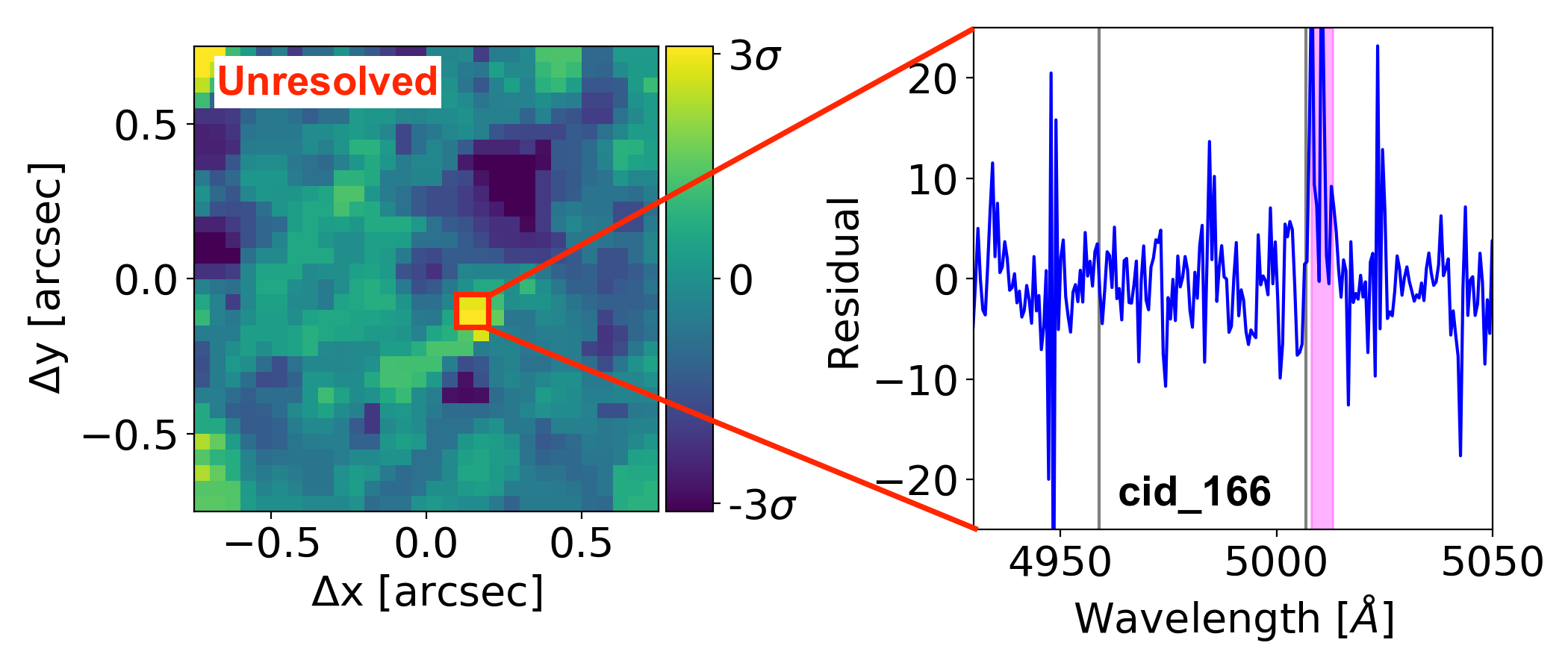
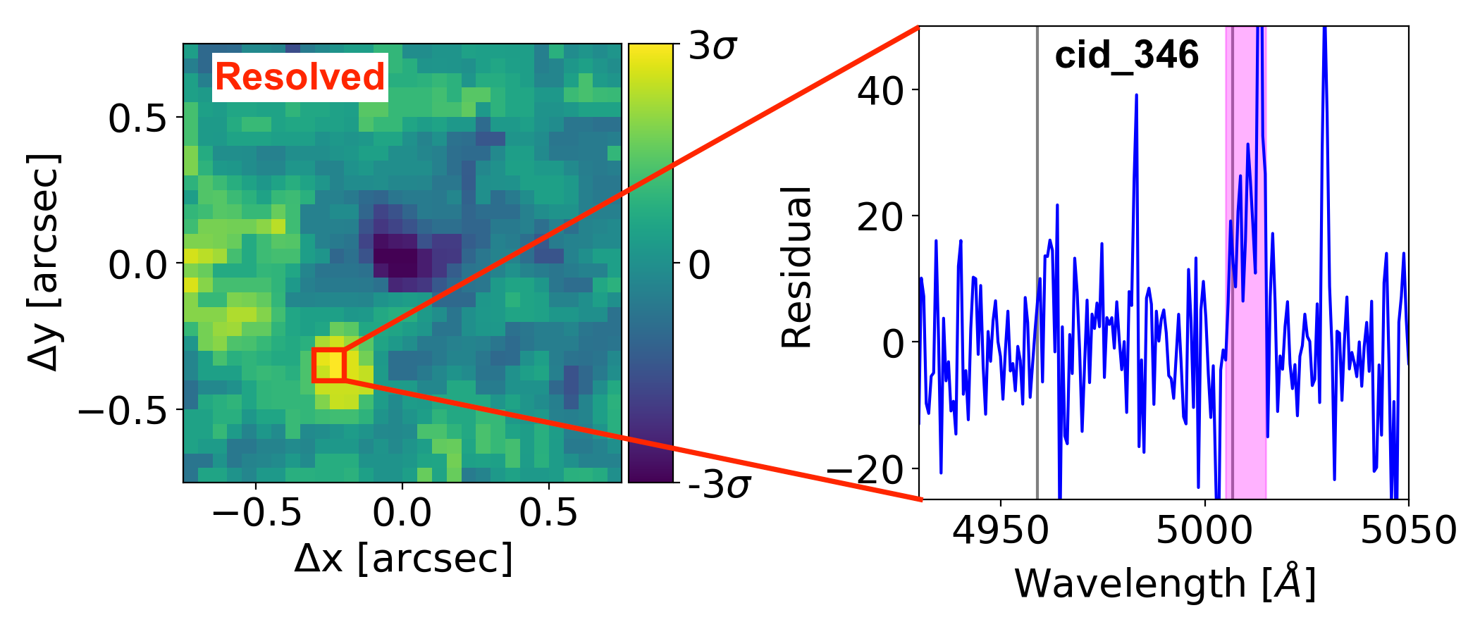
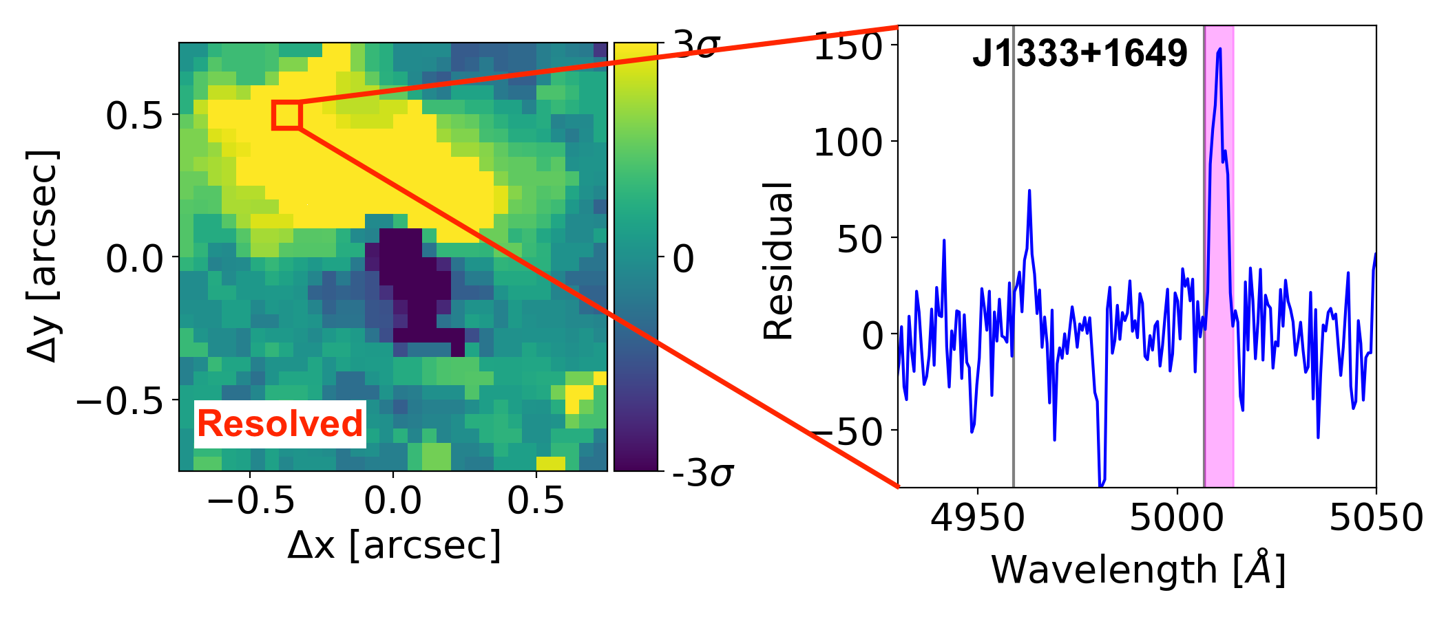
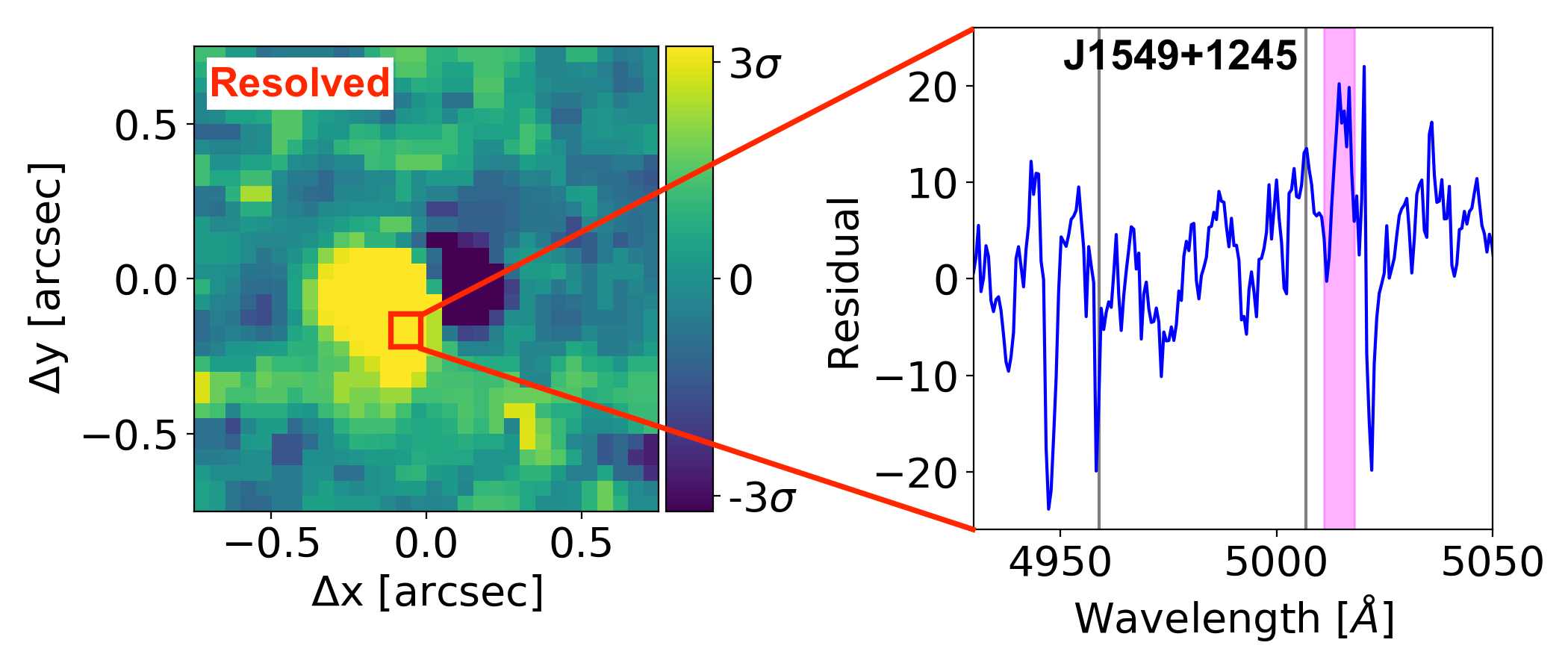
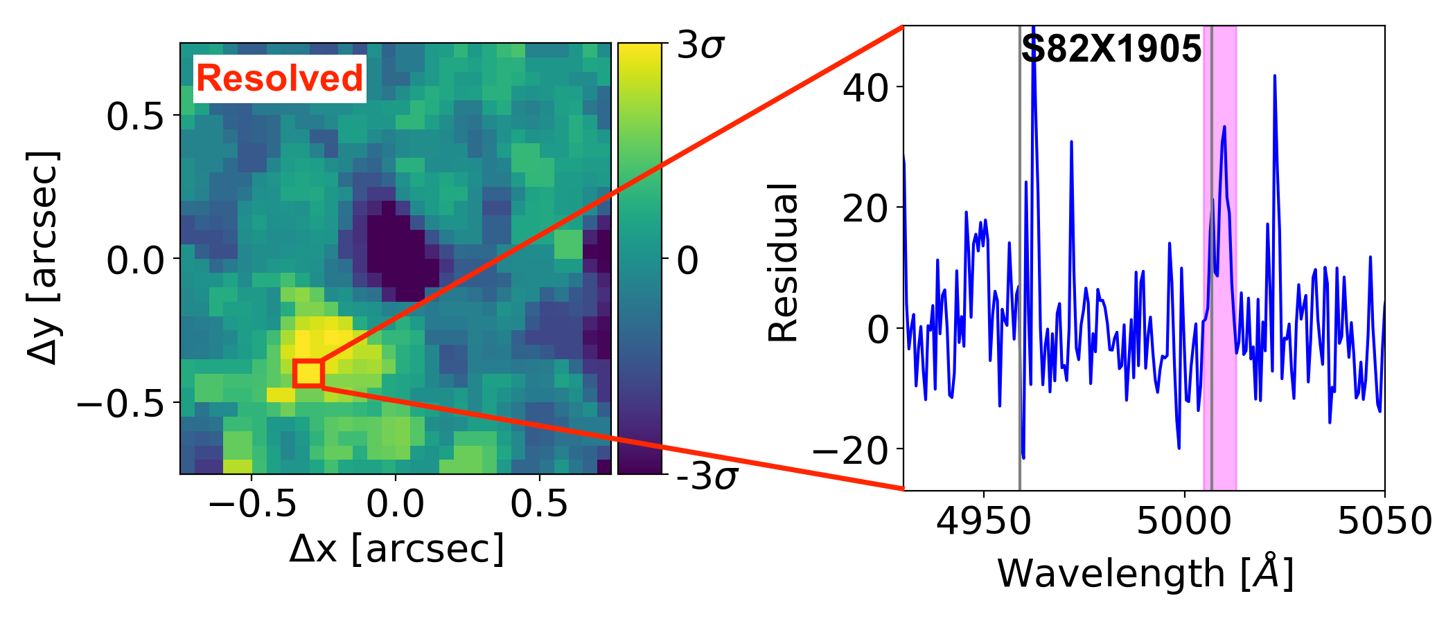
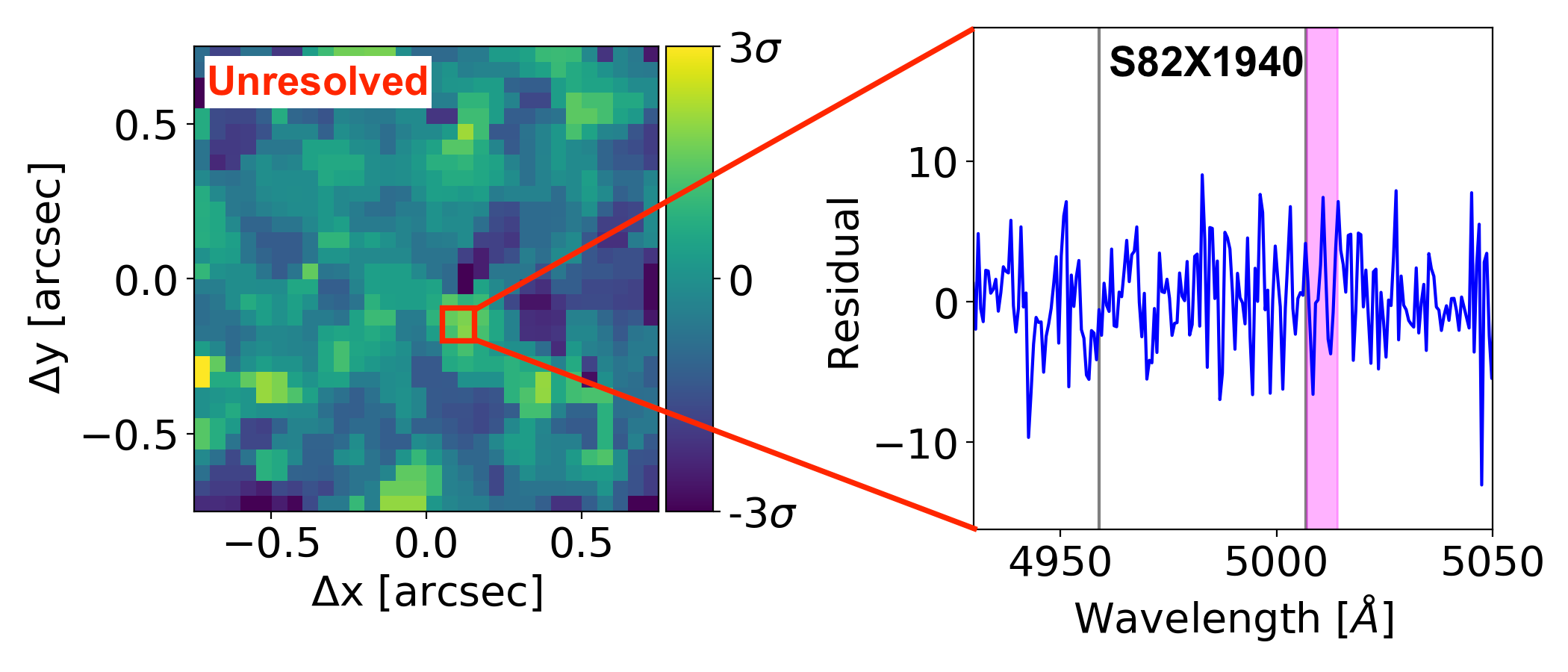
Figure 6: Residuals obtained using the ”PSF-subtraction” method across the SINFONI FoV as described in section 5 for the Type-1 sample. The left panel shows the residual image obtained by collapsing the channels at the location of [O iii] $\lambda$5007 after subtracting the emission from the AGN. The color map is on a linear scale with the yellow regions showing excess emission (i.e. $>3\sigma$). North is up and East is to left. The right panel shows the spectrum extracted at the location of excess emission, with an aperture of 0.1${}^{{}^{\prime\prime}}\times$0.1${}^{{}^{\prime\prime}}$ shown by the red square in the left panel. The vertical grey lines in the residual spectrum shows the location of the [O iii] $\lambda$4959 and [O iii] $\lambda$5007 respectively, while the channels used to create the residual map on the left are indicated with a magenta box. Non-zero residuals in the images show that [O iii] emission is resolved, while a noisy pattern is indicative of unresolved emission, which are respectively marked in the left panels. X_N_66_23 is not included in this analysis due to non-detection of the BLR component.

Before discussing the kinematics of the ionized gas, we now focus on the actual extension and morphology of the emission line region. First, we need to verify that the [O iii] emission is actually extended or rather unresolved and what it may erroneously be interpreted as extended emission being nothing else than beam smearing effects (e.g. Husemann et al., 2016; Villar-Martín et al., 2016). We use two techniques to asses if the emission is truly extended. The first consists in comparing the curve-of-growth (COG) of the total [O iii] emission of the AGN with that of an observed and modeled PSF. The second technique, which we will call ”PSF-subtraction” method, consists in producing a residual [O iii] map after subtracting the nuclear [O iii] spectrum spaxel-by-spaxel following a 2D PSF profile.

To construct the curves of growth, we start by extracting the spectrum from an aperture of radius 0.1^′′ centered at the peak location of the AGN continuum emission and perform the line fitting as described in Sect. 5.1. From the best fit we derive the flux value for the total [O iii] emission, and repeat this procedure increasing the extraction radius in steps of 0.05^′′. We finally reconstruct the curve of growth plotting the line fluxes derived as a function of the aperture radius. We only plot the total [O iii] flux and not the individual components in these plots as we do not give any physical significance to individual Gaussian components. The curves of growth are derived for 11 targets (out of the 21 in the Type-1 sample observed) for which the signal-to-noise in the integrated spectrum extracted from their respective apertures (Table 3) is greater than 5. The H-band data cubes of cid_1205 and S82X2058 are contaminated by a bright stripe, due to which spatially resolved analysis of these targets is not performed.

We then need to have an accurate description of the PSF to compare with the [O iii] emission. We had designed our SINFONI observations to have dedicated PSF star observations close in time and space for each single science observations, and we can therefore repeat the COG procedure described above for the AGN also for the dedicated PSF star, in order to derive the PSF profile as a function of the distance from the center. We were not able to construct the growth curve of PSF observation for J1333+1649 and J1549+1245 as the PSF star was at the edge of the data cube. Nevertheless, since the AGN in this paper are Type-1 we have access to the spatially unresolved BLR emission as traced by $\mathrm{H\beta}\leavevmode\nobreak\$ which we can use as an alternative method to trace the PSF profile (the only exception being X$\_$N$\_$66$\_$23 for which we do not have a clear detection of the $\mathrm{H\beta}\leavevmode\nobreak\$ line). Out of the eight objects for which we can use both methods to trace the PSF, both the dedicated PSF star and the $\mathrm{H\beta}\leavevmode\nobreak\$ BLR component give consistent PSF profiles for five objects so we can use both to trace the spatial resolution of the data cubes. For the remaining three objects (X_N_115_23, cid_346, S82X1905) the PSF profile as traced by the dedicated star observation is narrower than those derived from the $\mathrm{H\beta}\leavevmode\nobreak\$ profile. These differences between the PSF traced by the BLR emission and the PSF star could be due to the difference in the AO correction, which might change in long exposure observations. Also, as the PSF star observations were performed at the beginning of the $\sim 1$ hour long science OBs, for these three objects the conditions got relatively worse during the science observations and therefore we consider the PSF profile derived from the BLR the correct one to compare since they trace the conditions simultaneously with the science observations. We finally estimate errors on the COGs by repeating the fitting procedure 100 times on mock spectra obtained by adding rms errors on an object-free location of the spectrum on the original models. The curves of growth for the 11 targets with a S/N$>5$ in each apertures are presented in Fig. 5.

We can now compare the COG of each single target with the PSF. As discussed above whenever possible we consider the PSF curve obtained from the unresolved BLR the best representations of the observing conditions during the science observations. From Fig. 5 we find that for 7 targets ($\approx$ 63% of the targets for which this analysis has been performed) there is a 2$\sigma$ excess in the total [O iii] emission compared to the PSF at the maximum radius sampled by the COG, and therefore we will claim that in these objects the [O iii] is spatially resolved. As done also in previous works, we could compare the half light radii (the radius containing $50\%$ of the flux) of the [O iii] and the PSF emission reported in Table 4 to asses the spatially resolved nature of the [O iii] emission. The half light radii were estimated using linear spline to interpolate between the data points of COG. For five objects (X_N_66_23, X_N_115_23, cid_346, J1549+1245 and S82X1905) the [O iii] half light radius is larger than the PSF half light radius within $\approx$2$\sigma$. For the remaining targets the COG of the [O iii] emission and the half light radius is consistent with the PSF within 2$\sigma$. In particular, for the two targets X_N_81_44 and J1333+1649 the half-light radius method may not be sensitive to the fainter very extended emission beyond the PSF, contrary to the overall COG and PSF-method described below.

As mentioned at the beginning of this section, we use a second method to asses the spatial extension of the ionized gas emission, namely the “PSF-subtraction” method as described in Carniani et al. (2015). The basic principle behind the PSF-subtraction method is that if the observed emission is unresolved and/or is a result of beam smearing from the PSF of the AGN, the spectrum at any given distance from the location of the AGN is the same as the spectrum at the location of the AGN, except for a scaling factor across the spectrum (e.g. Jahnke et al., 2004). In this case, the BLR component of $\mathrm{H\beta}\leavevmode\nobreak\$ smears the emission across the FoV and is therefore AGN dominated. If the emission does not mimic the spectrum at the location of AGN, then the observed spectral line is resolved. Following this principle for our sample, we first model the spectrum extracted at the AGN location (within a radius of 0.1^′′), determined using the center of the continuum in the H-band cube. We will refer to this spectrum as the “nuclear model” which we then subtract from every pixel across the SINFONI FoV, after allowing a variation in the overall normalization factor of the spectrum while keeping the rest of the kinematic components fixed. This is followed by creation of channel maps at the location of [O iii] $\lambda$5007 emission in the nuclear-spectrum-subtracted cube. The channels used to create the residual maps were 6$\AA$ wide, except cid_346 for which a channel width of 10$\AA$ was used. Following the principle described above, a noisy residual map will indicate an unresolved emission, while a map with structures having non-zero residual will indicate a resolved emission. Similar to the case of the COG, we restrict this analysis only to targets which have a S/N larger than 5 in the integrated spectrum (extracted from the respective apertures reported in Table 3). We also restrict the analysis to targets which show BLR $\mathrm{H\beta}\leavevmode\nobreak\$ emission which is used to scale the overall normalization of the nuclear spectrum. Since we do not detect a BLR component in X_N_66_23, we perform the PSF-subtraction analysis for 10 SUPER targets. The results of this method are shown in Fig. 6. The left panels in these figures show the residual maps obtained after collapsing the nuclear-spectrum subtracted cubes along the [O iii] channels, while the right panels show the residual spectrum extracted at the region of excess emission. From Fig. 6, we see excess residuals at a level of ¿2$\sigma$ for 6 SUPER targets - X_N_81_44, X_N_115_23, cid_346, J1333+1649, J1549+1245 and S82X1905.

In summary, from the joint analysis based on the COG and ”PSF-subtraction” method we have identified seven sources from our sample which show extended [O iii] emission. Further analysis on the spectra across the SINFONI FoV will therefore be restricted to the 7 targets, which show extended gas emission with at least one of the methods described above.

5.3 Modeling ionized gas kinematics across the FoV

In the following section, we describe the pixel-by-pixel analysis for the H-band raw data cubes of the 7 targets which are resolved from the methods described in Sect. 5.2. For the modeling of the spectrum across every pixel, we use the parameters obtained in the integrated spectrum as a prior. Apart from the constraints set while modeling the integrated spectrum, we also fix the centroid and the width of the unresolved BLR component of $\mathrm{H\beta}\leavevmode\nobreak\$ and only allowed a variation in its peak. In the H-band, the Gaussian parameters of other emission lines are allowed to vary. The emission line widths (FWHM) were also kept greater than $\sim$100 km/s to avoid any spurious fit to a sky line. The validity of the line fitting across each spaxel was checked by subtracting the emission line model from the raw data and making a collapsed map along the channels spanned by the [O iii] $\lambda$5007 emission. Due to the low S/N in each spaxel in case of X_N_66_23 and cid_346, nearby spaxels were averaged within a radius of 0.1^′′ to produce binned spectra. This results in a higher S/N of the spaxels without compromising the respective resolution of the observations.

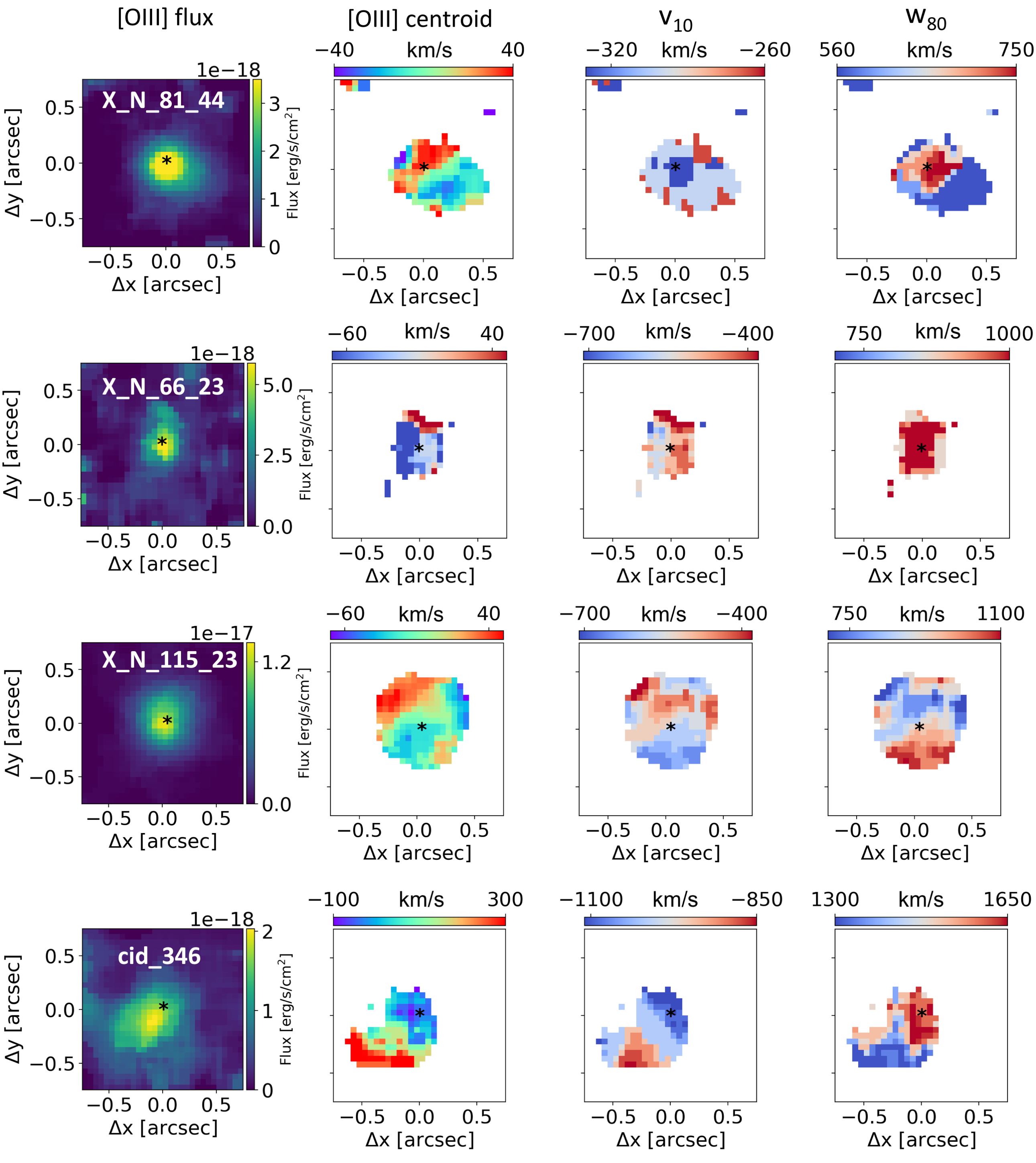
(a)

Figure 7: Flux and velocity maps of the targets showing resolved/extended emission inferred from the curve-of-growth and PSF-subtraction method (From top to bottom: X_N_81_44, X_N_66_23, X_N_115_23 and cid_346). Column 1: Background image shows the flux map of total [O iii] emission (narrow+broad).; Column 2: [O iii] line centroid map; Column 3: $\mathrm{v_{10}}$ map and Column 4: $\mathrm{w_{80}}$ map. In all the maps, the black star denotes the center position of the H-band continuum, as a proxy for AGN location. North is up and East is to left.

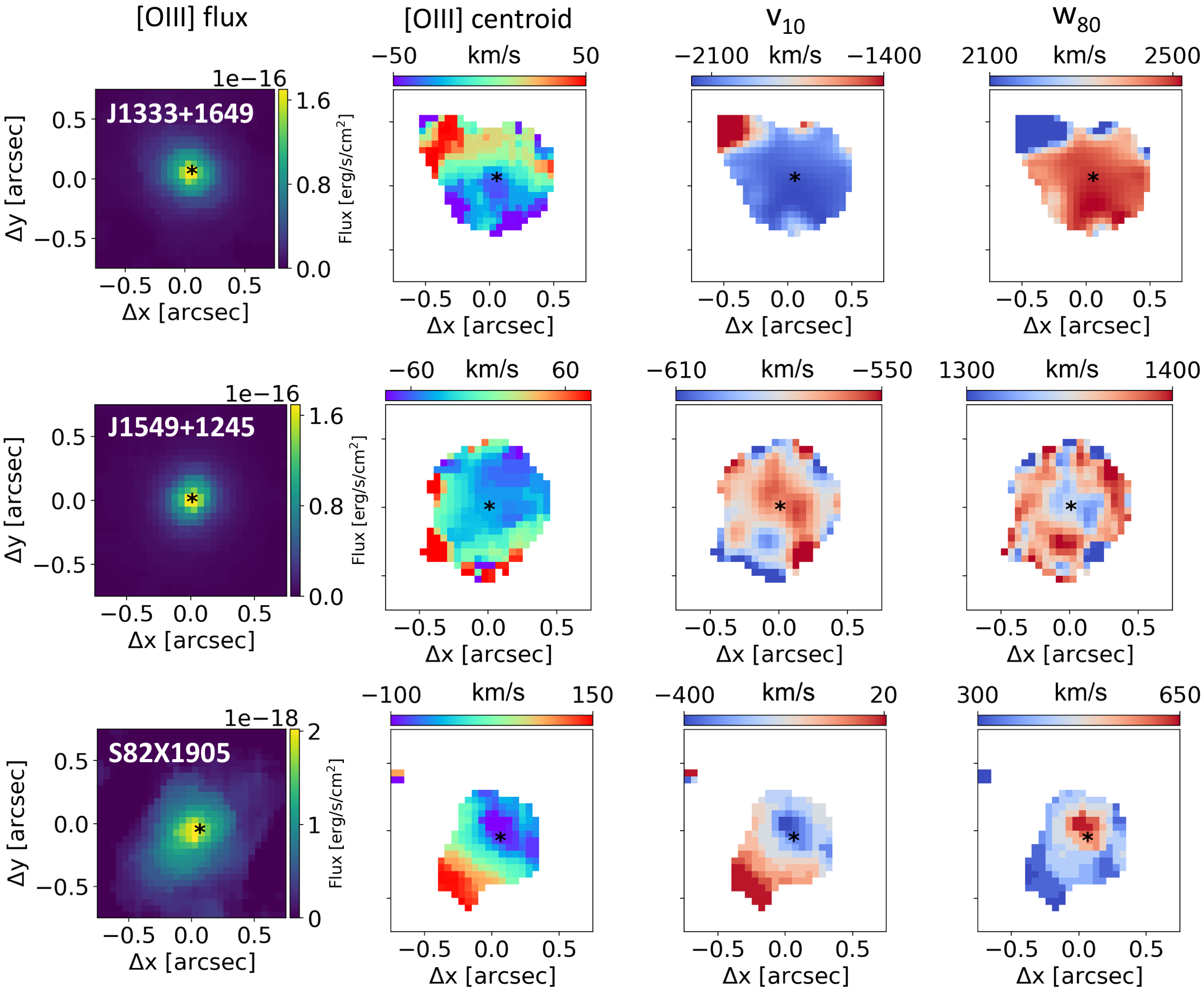
(a)

Figure 8: Same as Fig. 7 for J1333+1649, J1549+1245 and S82X1905.

As a result of the pixel-by-pixel analysis, various line and continuum maps are created which we describe below. These maps are shown in Figs. 7 and 8. All the maps are smoothed to the spatial resolution of the observations derived from the PSF and a S/N cut of 2 is employed in the [O iii] profile. First, we created broad band continuum maps, masking the emission lines, and used a 2-D Gaussian fit to determine the photo-centroid of the resulting image which we will use to mark the AGN position.

The total [O iii] line flux maps are shown in the first column of Figs. 7 and 8, while the line centroid maps obtained from the peak of the total [O iii] profile are presented in the second column. A smooth gradient is observed in some of the line centroid maps, e.g. in X_N_81_44, X_N_66_23, cid_346 and S82X1905, which could be indicative of a rotating disk in the host galaxy or a bi-polar ionized outflow. The observed extreme high velocities in the $\mathrm{w_{80}}$ maps ($\sim$1000 km/s) for most of these galaxies suggest that the kinematics of the ionized gas are also likely affected by the central AGN. For several of our targets, we do detect extended features in emission, which are not produced by wings of the PSF as demonstrated by the analysis performed in the previous sections (e.g. X_N_115_23, CID_346, J1333+1649, J1549+1245, S82X1905). A possible explanation for these irregular features in the gas kinematics could be the presence of a merger event between two galaxies. As far as a major merger is concerned, we do not see clear evidence of multiple galaxies in the available ancillary data. We would, therefore, favor alternative scenarios in which the extended features could be interpreted as an inflow or outflow. Inflows are usually detected in absorption and are predicted to show lower velocities than what we measure for the SUPER sample (e.g. Bouché et al., 2013). Also, since models predict a low covering fraction for the inflows (e.g. Steidel et al., 2010), we are inclined to interpret these features as outflows. In order to further investigate the kinematic features of the ionized gas in these AGN, we also generated the maps with the spatial variation of $\mathrm{v_{10}}$ and $\mathrm{w_{80}}$ which are shown in the third and the fourth column in Figs. 7 and 8. The inspection of both maps reinforces our conclusion that most of our objects do not present the kinematic signatures of an undisturbed rotating disk: the $\mathrm{v_{10}}$ map shows regions with extremely blue shifted velocity of more than -1000 km/s with $\mathrm{w_{80}}$ that peaks at the location of maximum velocity shift. Although a proper modeling of the velocity field of these galaxies is beyond the scope of this paper, we will discuss here the morphology and size of the outflows signatures.

Following the discussion of the integrated spectra in Sec 5.1, we will use the cut $\mathrm{w_{80}}>$600 km/s to identify regions dominated by outflowing ionized gas. Projected velocities (e.g. $\mathrm{v_{10}}$ maps in the third column in Figs. 7 & 8) will be more sensitive to the galaxy inclination while the $\mathrm{w_{80}}$ maps are more likely to be less sensitive to inclination (e.g. see discussion in Harrison et al. 2012). For each source, we measure the maximum projected spatial extent of the $\mathrm{w_{80}}>$600 km/s component of the [O iii] line profile (we will name this quantity D₆₀₀, following Harrison et al. 2014). From the $\mathrm{D_{600}}$ values in the $\mathrm{w_{80}}$ maps we find that the outflows are extended from $\sim$2 kpc up to 6 kpc (see Table 4).

Table 4: Properties of the ionized gas obtained from the analysis of the curves-of-growth, spectroastrometry and the flux and velocity maps. J1441+0454 has not been mentioned in this table due to the lack of [O iii] emission.

Target	$\mathrm{r_{1/2}^{[{O\textsc{iii}}]\leavevmode\nobreak\ }}$	$\mathrm{r_{1/2}^{PSF}}$	$\mathrm{v_{o}}$	$\mathrm{R_{o}}$	$\mathrm{D_{600}}$	$\mathrm{L_{[{O\textsc{iii}}]\leavevmode\nobreak\ }^{o}}$	$\mathrm{\dot{M}_{cone}}$	$\mathrm{\dot{M}_{thin-shell}}$	$\mathrm{f_{esc}}$
	(1)	(2)	(3)	(4)	(5)	(6)	(7)	(8)	(9)
	kpc	kpc	km/s	kpc	kpc	erg/s	$\mathrm{M_{\odot}/yr}$	$\mathrm{M_{\odot}/yr}$	%
X_N_160_22	1.54$\pm$0.02	1.52$\pm$0.02	-1700	0.4	–	43.36	4–79	5–105	38
X_N_81_44	1.84$\pm$0.16	1.61$\pm$0.05	+500	0.9	2.4	42.26	0.1–1	0.1–2	6
X_N_66_23	1.29$\pm$0.12	1.03$\pm$0.02	600	0.4	2.4	42.88	0.4–7	0.5–10	4
X_N_35_20**	–	–	681	¡2.2	–	41.31	0.01–0.2	0.01–0.2	0
X_N_12_26	1.08$\pm$0.07	1.14$\pm$0.01	-400	0.3	–	42.06	0.1–1	0.1–2	2
X_N_4_48*	–	–	1198	¡2.9	–	41.97	0.1–1	0.1–2	5
X_N_102_35*	–	–	1501	¡7.6	–	42.68	0.4–9	0.6–12	16
X_N_115_23	1.67$\pm$0.04	1.49$\pm$0.04	+900	0.9	4.0	43.09	0.3–6	0.4–8	7
cid_166	1.42$\pm$0.03	1.42$\pm$0.02	-2100	0.7	–	43.10	1–27	2–36	30
cid_1605*	–	–	1153	¡5.8	–	42.15	0.1–2	0.1–3	4
cid_346	2.12$\pm$0.07	1.90$\pm$0.05	+600	2.8	5.6	42.83	0.6–11	0.8–15	27
cid_1205†	–	–	717	¡2.5	–	42.08	0.05–1	0.1–1	0
cid_467*	–	–	1368	¡9.0	–	42.63	0.4–7	0.5–10	8
J1333+1649	1.76$\pm$0.03	1.74$\pm$0.05	-2900	0.3	6.5	44.54	51–1021	68–1361	43
J1441+0454**	–	–	2161	¡2.8	–	43.41	3–68	4–91	97
J1549+1245	1.35$\pm$0.03	1.25$\pm$0.03	+1300	0.2	4.0	44.29	16–326	22–435	12
S82X1905	1.86$\pm$0.04	1.73$\pm$0.01	+300	2.7	1.6	42.21	0.04–0.8	0.1–1	0
S82X1940	1.23$\pm$0.03	1.29$\pm$0.04	-600	0.6	–	42.35	0.2–3	0.2–4	8
S82X2058†	–	–	1340	¡2.2	–	42.54	0.3–6	0.4–8	13

Notes: (1) & (2): $\mathrm{r_{1/2}^{[{O\textsc{iii}}]\leavevmode\nobreak\ }}$ and $\mathrm{r_{1/2}^{PSF}}$ are the half-light radius of the BLR PSF and [O iii] emission respectively, derived from the curve-of-growth analysis for 11 targets with S/N¿ 5 in the integrated spectrum of [O iii] , as described in Sect. 5.2. ${}^{**}\mathrm{r_{1/2}^{[{O\textsc{iii}}]\leavevmode\nobreak\ }}$ is not computed for X_N_35_20 and J1441+0454 as the [O iii] S/N is low. Targets marked by * were observed without AO and are not resolved. H-band data cubes of cid_1205 and S82X1058 (marked by ^†) have a bright stripe which interferes in the spatially resolved analysis and therefore the half-light radius have not been reported (see Sect. 5.1).
(3) & (4): $\mathrm{v_{o}}$ is the outflow velocity of the bulk of the ionized gas, which is at the maximum distance, $\mathrm{R_{o}}$ , from the AGN. $\mathrm{v_{o}}$ and $\mathrm{R_{o}}$ are derived from the spectroastrometry analysis of the 11 targets with S/N¿5 in the integrated spectrum of [O iii] , as described in Sect. 5.4. For targets marked by *, ** or ^†, we report the $\mathrm{w_{80}}$ value of the integrated spectrum and the PSF value as a proxy for $\mathrm{v_{o}}$ and $\mathrm{R_{o}}$.
(5): D₆₀₀ is the maximum projected spatial extent of $\mathrm{w_{80}}$ ¿ 600 km/s from the maps in Figs. 7 and 8. D₆₀₀ is calculated for 7 targets which show extended ionized gas emission from COG and PSF-subtraction methods.
(6): $\mathrm{L_{[{O\textsc{iii}}]\leavevmode\nobreak\ }^{o}}$ is the outflow luminosity computed from [O iii] $\lambda$5007 emission line for channels with —v—¿300 km/s (Sect. 5.5).
(7) & (8): $\mathrm{\dot{M}_{cone}}$ and $\mathrm{\dot{M}_{thin-shell}}$ are the masss outflow rates assuming a bi-conical and a thin-shell geometry described in Sect. 5.5. The two values in each column correspond to the outflow rates assuming an electron density of 10⁴ cm^-3 and 500 cm^-3.
(9): $\mathrm{f_{esc}}$ is the fraction of the outflowing gas which has the capability to escape the gravitational potential of the host galaxy (Sect. 6).

From the $\mathrm{w_{80}}$ maps in Figs. 7 and 8, it is clear that the ionized outflows detected in these AGN present a diversity of projected structures. In five sources (X_N_81_44, X_N_115_23, cid_346, S82X1905) there is a velocity gradient along a particular axis while for two objects (J1333+1649 and J1549+1245) the maps are more spherically symmetric. Some of the kinematic structures present in the $\mathrm{w_{80}}$ maps could be consistent with a bi-conical outflow, where the inclination of the outflow with respect to the disk of the galaxy and the line-of-sight of the observer could explain the observed velocity maps: i.e. a high inclination of the outflow with respect to the line-of-sight will result in a clear velocity gradient along the outflow axis, with possibly both the blue-shifted and red-shifted part of the outflowing gas detected; a low inclination of the outflow with respect to the line of sight would produce a more uniform and spherically symmetric velocity field. A proper kinematic modeling would be required to constraint the ionized gas kinematics, and we will present this analysis in an upcoming paper on the full survey sample.

5.4 Radial distance of high-velocity ionized gas using Spectroastrometry

The analysis presented in section 5.2 is useful in determining the presence or absence of extended ionized gas. However, the methods described there do not determine the bulk velocity of the observed extended gas i.e. if the extended component of the gas is in outflow. Conventionally, the velocity maps derived in section 5.3 have been used to quantify the extension of the outflowing gas. These maps can only be used for targets which are well extended beyond the width (FWHM) of the observed PSF. For marginally resolved or unresolved targets, the velocity maps can be affected by PSF smearing. For the latter case, the spectroastrometry technique (Carniani et al., 2015) is useful to determine the radial distance of the bulk of the gas moving at certain velocity from the AGN location.

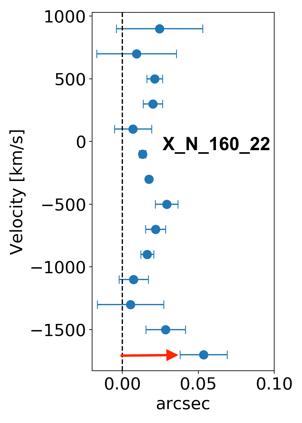
(a)

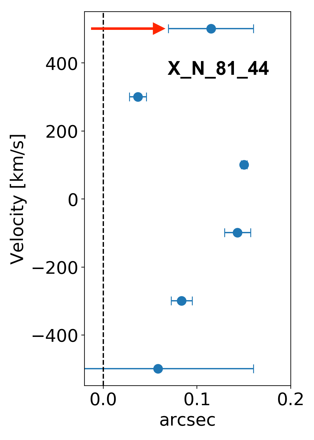
(b)

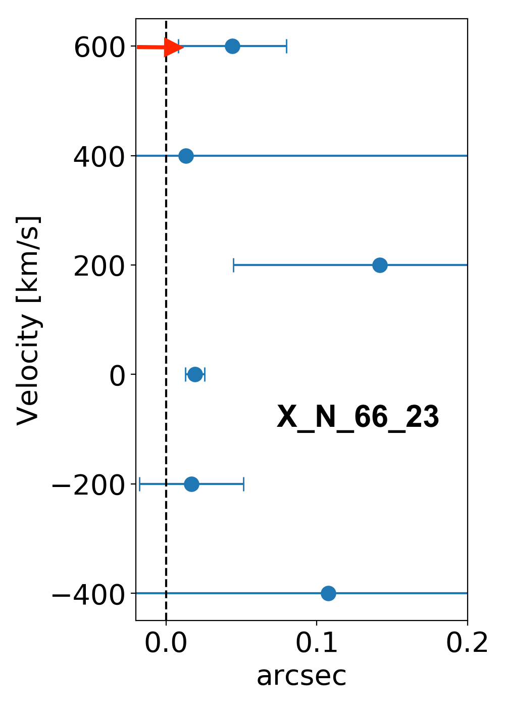
(c)

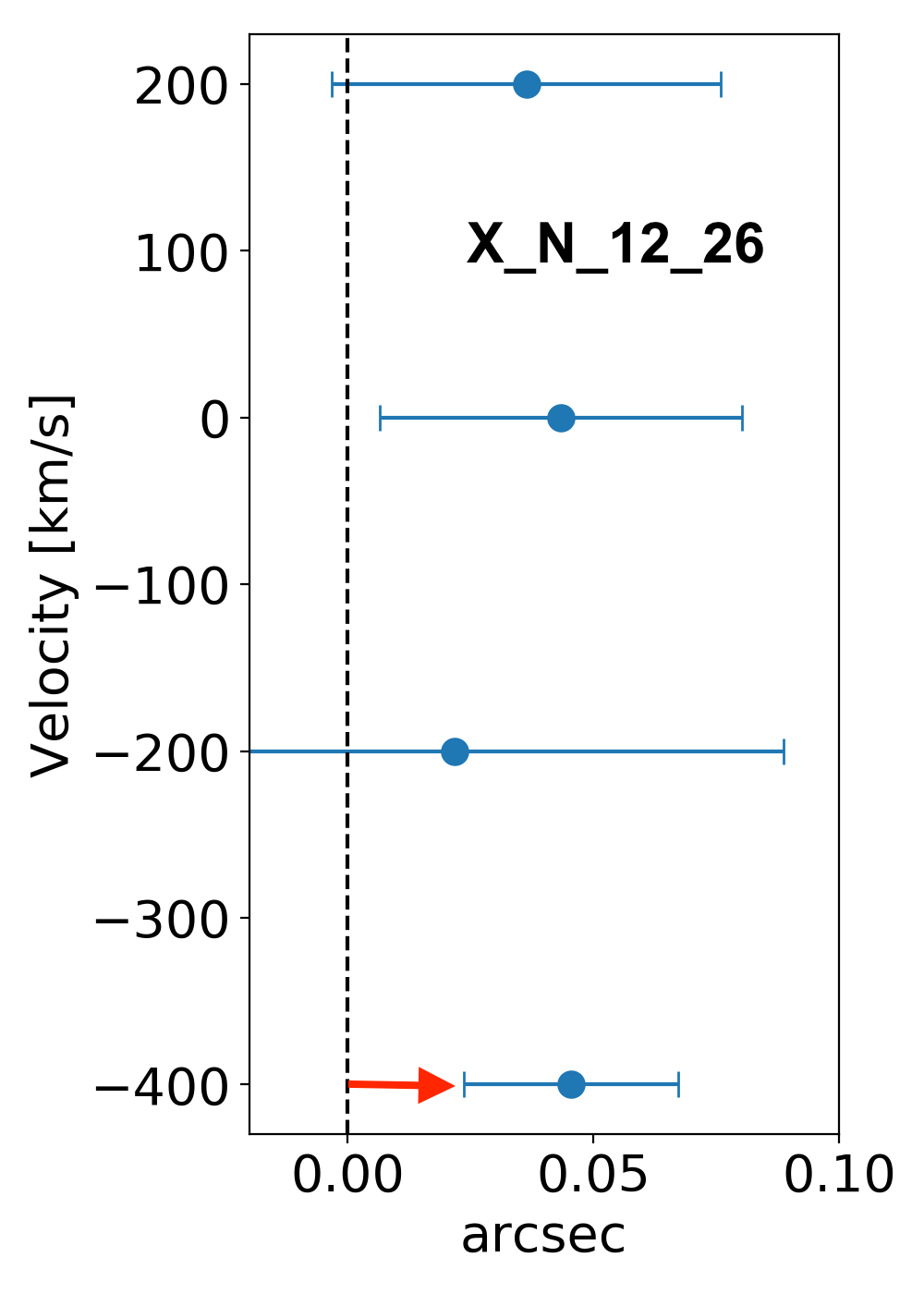
(d)

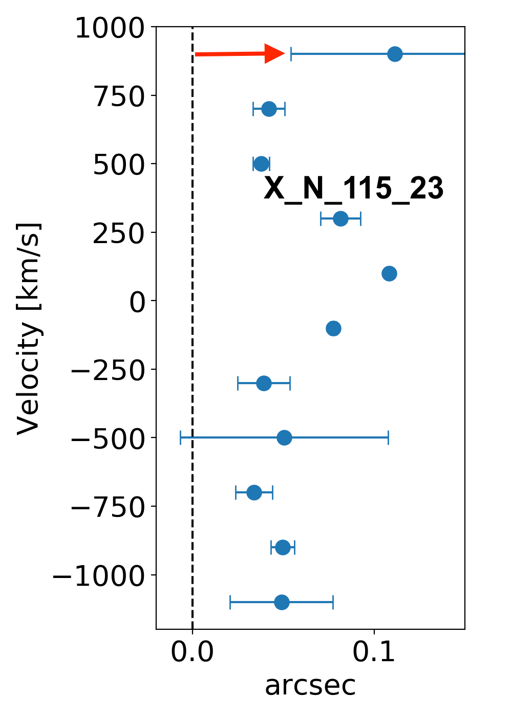
(e)

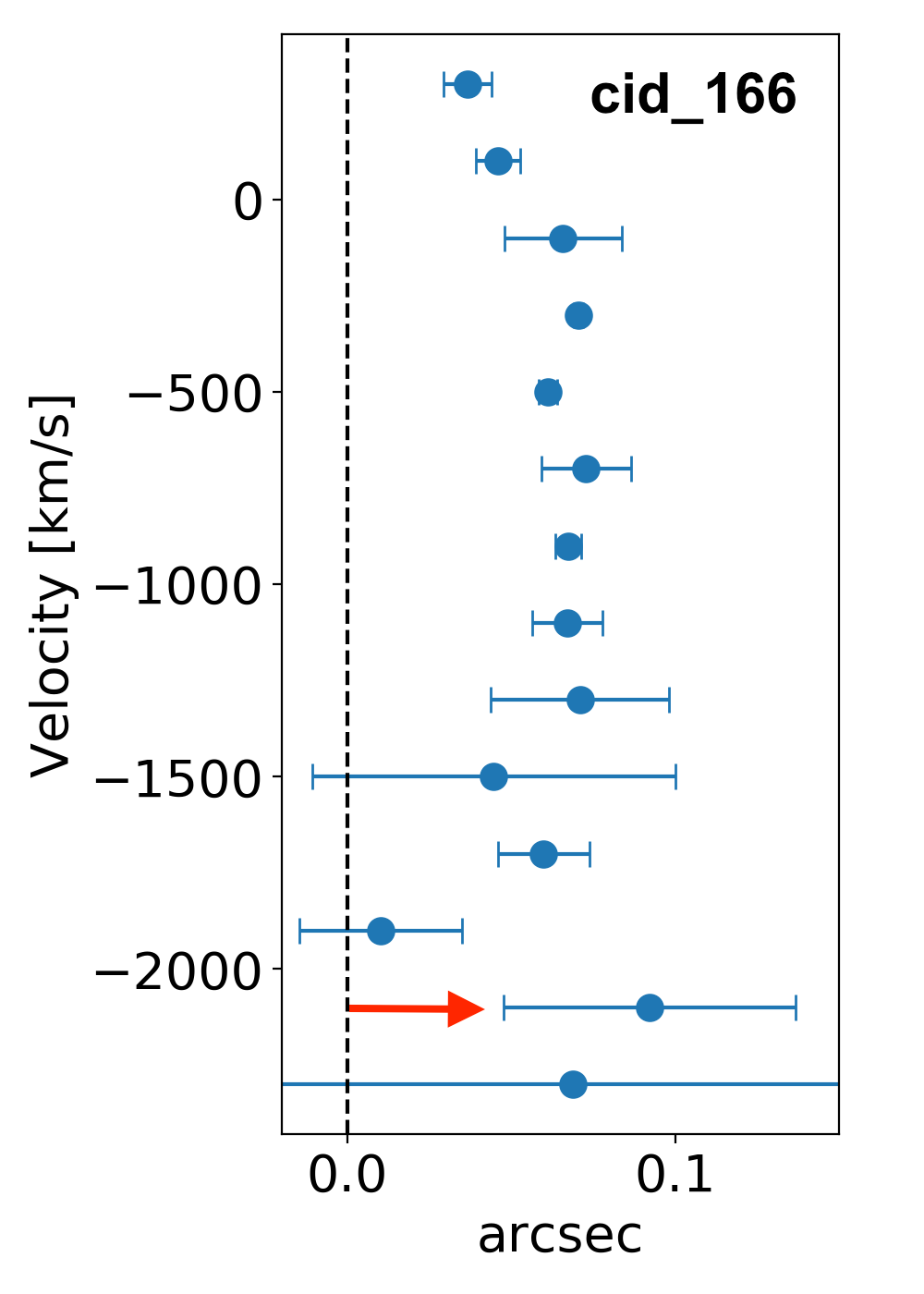
(f)

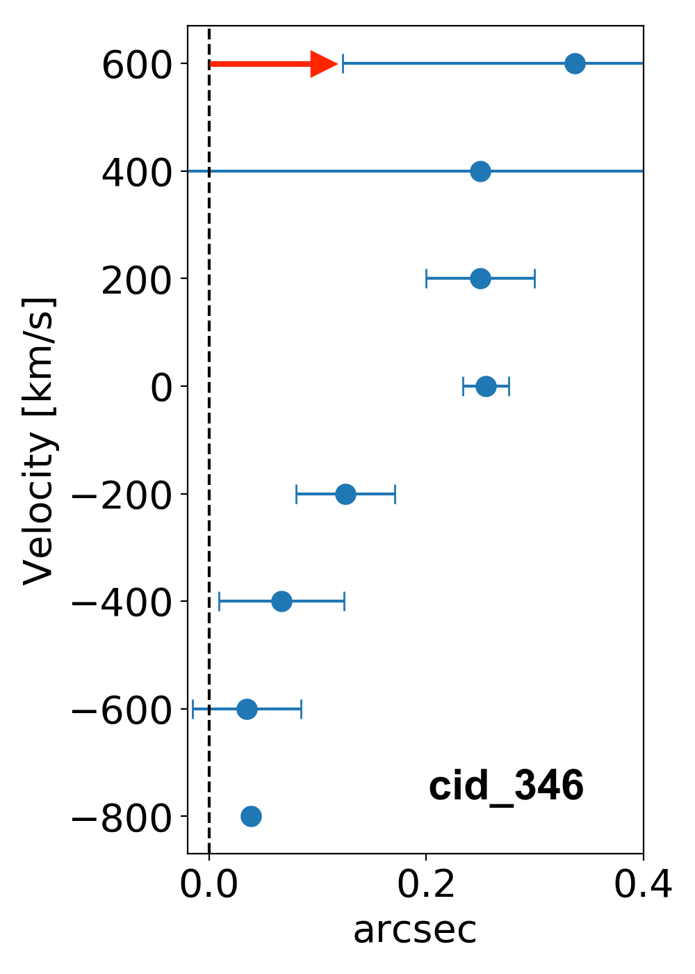
(g)

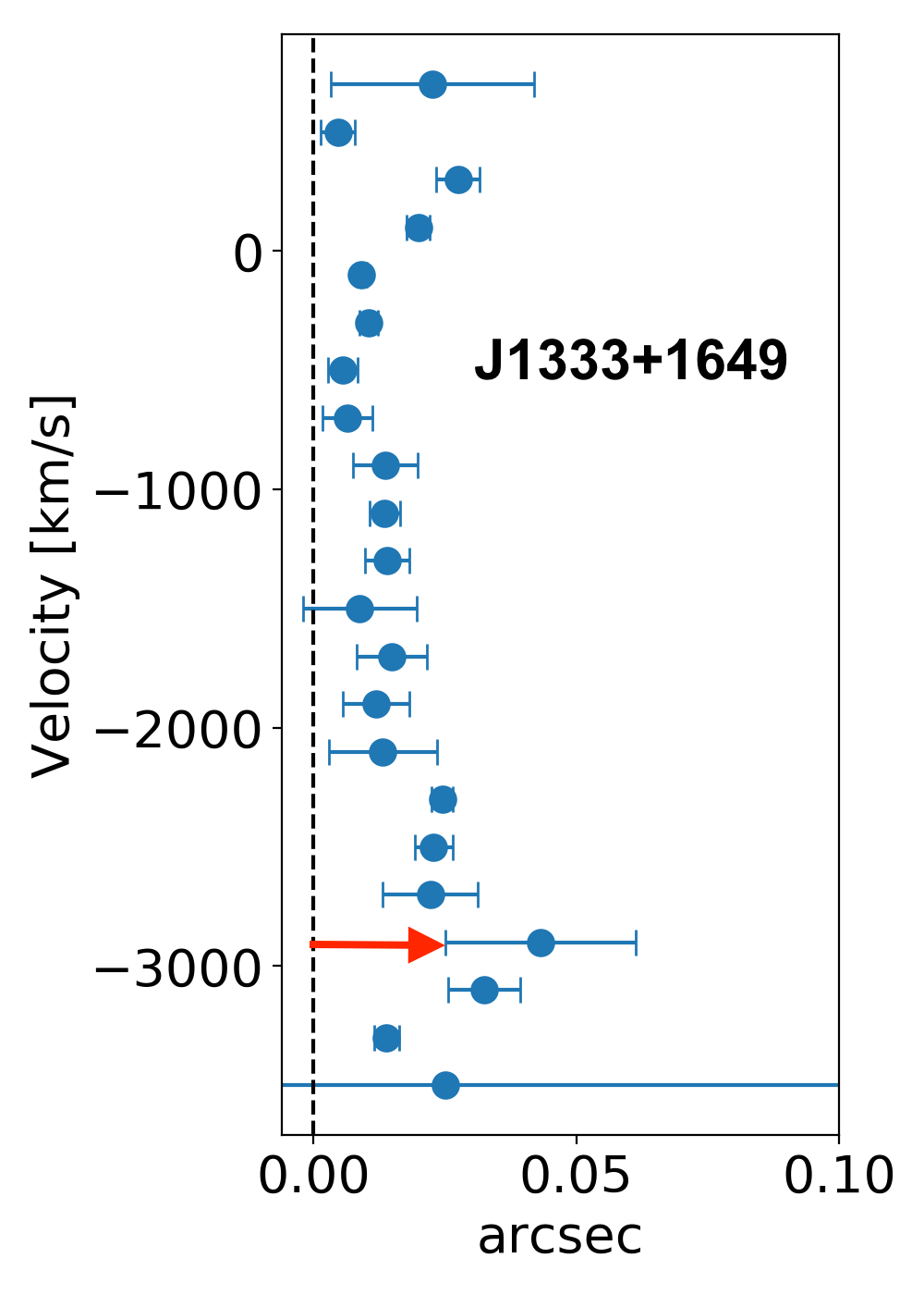
(h)

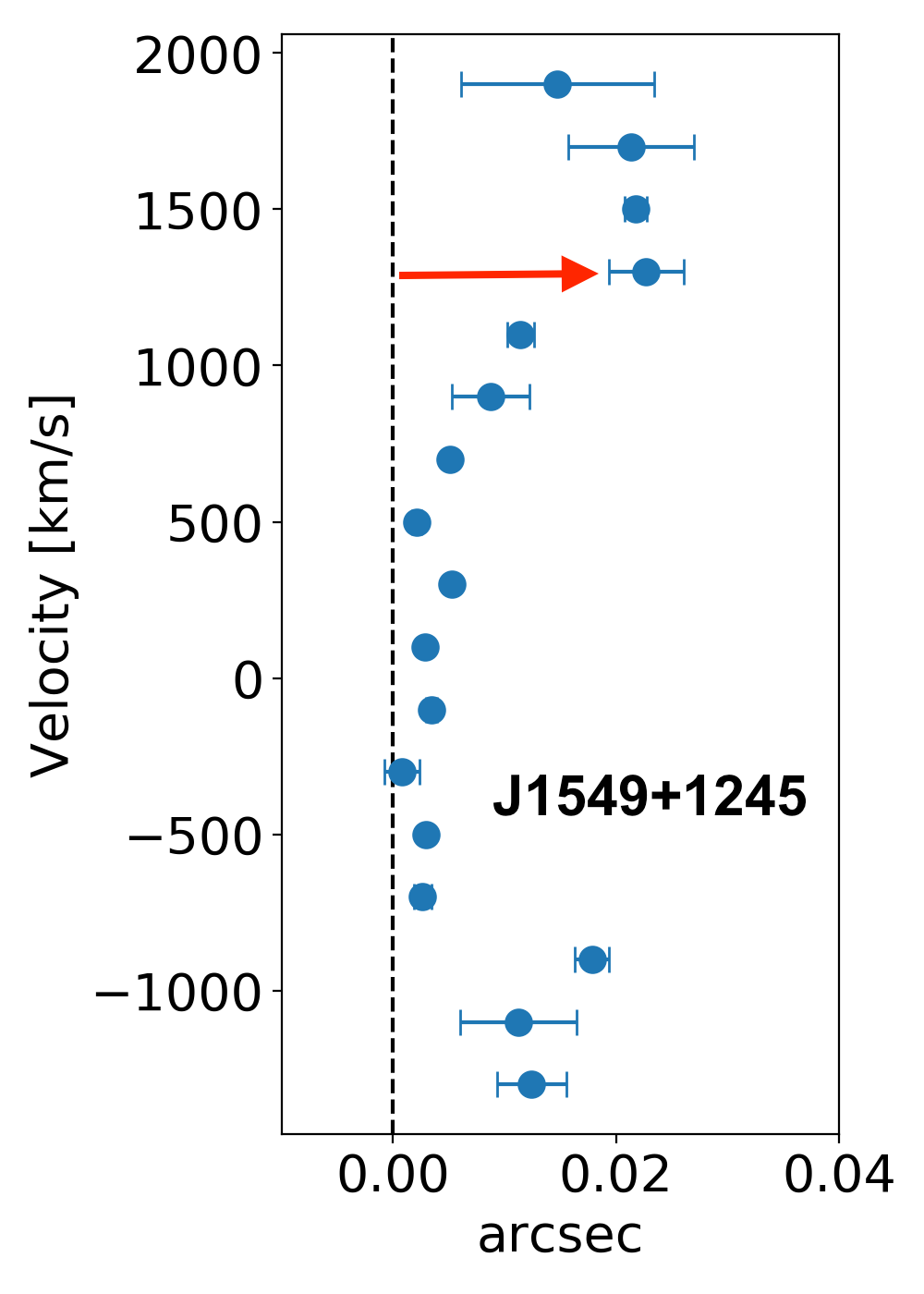
(i)

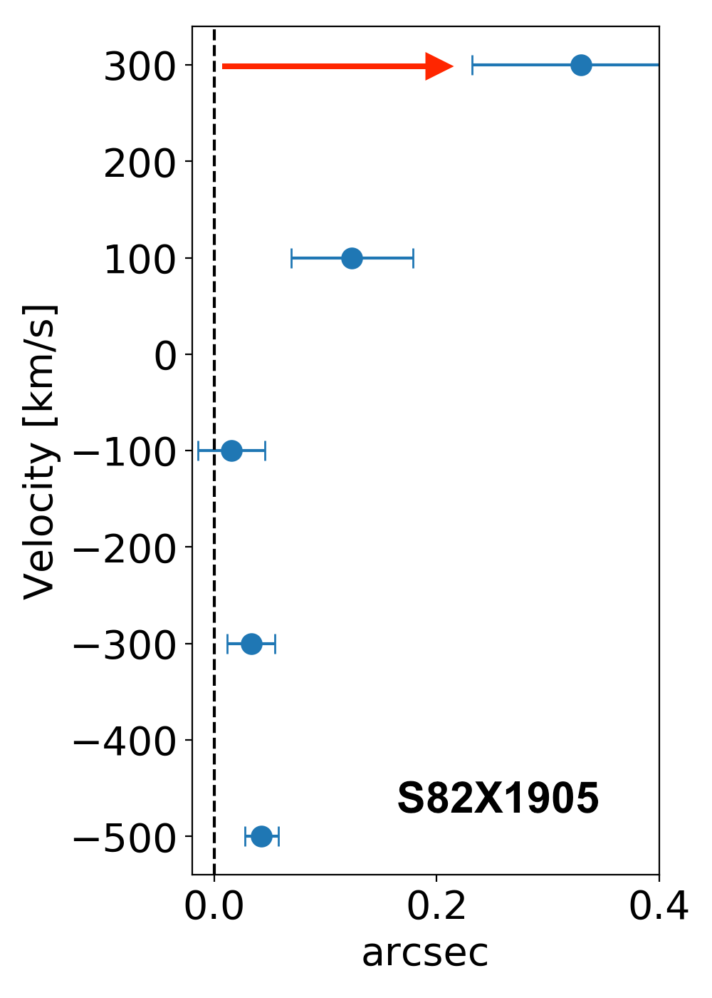
(j)

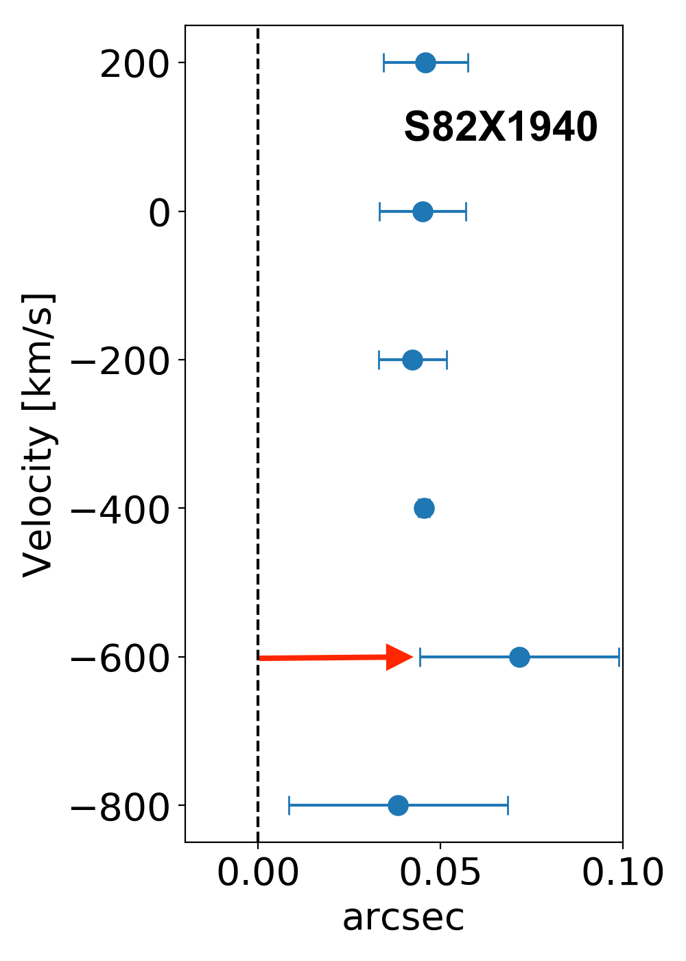
(k)

Figure 9: Results of spectroastrometry applied on the type-1 SUPER targets. The X-axis represents the distance between the continuum center (vertical dashed line) and the position of the photo-center of the [O iii] line at the corresponding velocity channel given in the Y-axis. The error bars represent 1$\sigma$ uncertainty on the values. The red arrow marks the cloud with velocity greater than 600 km/s (300 km/s in the [O iii] line profile) whose centroid is at the maximum distance from the AGN.

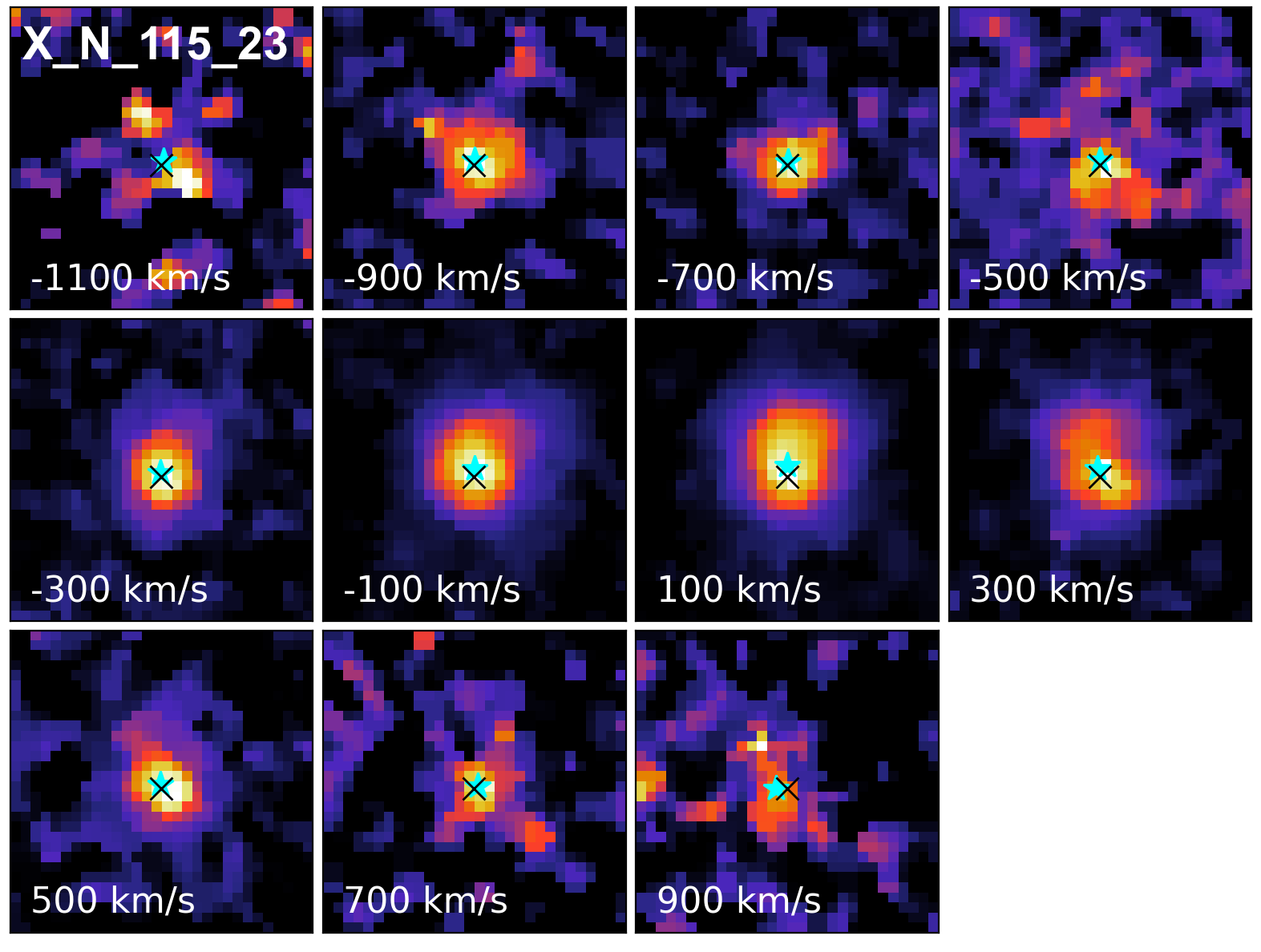
(a)

Figure 10: 1.5^′′ x 1.5^′′ [O iii] $\lambda$5007 channel maps of X_N_115_23 at different velocity slices, after subtracting the $\mathrm{H\beta}\leavevmode\nobreak\$, [O iii] $\lambda$4959 and iron models from the raw cube. Each velocity slice is 200 km/s wide and the displayed value is the center velocity of the respective channel. Black cross marks the location of the H-band continuum peak, used as a proxy for the AGN position and the cyan star marks the location of the [O iii] centroid determined from a 2-D Gaussian fit. North is up and East is to the left.

The principle of the spectroastrometry technique is that if the gas is moving at a distance R from the AGN position at a velocity different than the systemic velocity of the host galaxy (systemic here is defined by the position of the peak of the [O iii] line in the spectrum), then the photo-centroid of the line at that velocity is also shifted by a distance R from the AGN position. In this method, we first collapse the original data cube along channels containing AGN continuum and the photo-centroid of the resulting image is determined with a 2-D Gaussian fit, similar to the method described in Sect. 5.3. The photo-centroid of the continuum is used as an indicator of the AGN location. We then use the spectrum models derived in section 5.3 to subtract all the components from the raw spectrum across every pixel except those of the [O iii] $\lambda$5007. The resulting cube containing only the [O iii] $\lambda$5007 emission is then collapsed along wavelength channels with [O iii] emission in bins of $\sim$200 km/s such that we achieve a S/N of $\sim$2 in the [O iii] flux for each spectral channel. Similar to the continuum image, we then calculate the photo-centroid of each of the images obtained from the collapsed channels using a 2-D Gaussian fit. The velocity bins of $\sim$200 km/s ensures there are minimal errors in determining the centroid due to the spectral resolution of the instrument. The distance between the photo-centroid in each velocity channel and the AGN location is then plotted as a function of the center velocity of the channels. Note that spectroastrometry does not calculate the size of the outflowing gas but the spatial offsets between ionized gas clouds at different velocities with respect to the systemic velocity of the host galaxy. The offsets can be measured at scales smaller than the spatial resolution of the observations, and therefore the method can provide the distance of the bulk of the gas moving at a given velocity in unresolved or marginally resolved targets.

We apply the spectroastrometry method to all the 11 SUPER Type-1 AGN which have S/N ¿ 5 in the [O iii] line of the integrated spectrum. The results from the spectroastrometric analysis are shown in Fig. 9. The blue data points show the measured offsets from the AGN location, marked by the vertical dashed line at R = 0. The errors shown in the plot are the 1$\sigma$ uncertainty obtained from the output of the 2-D Gaussian fitting procedure. For each target we also produced the corresponding maps for each velocity channel included in the spectroastrometry analysis. Fig. 10 shows the channel maps for X_N_115_23 as an example, while the channel maps for the rest of the targets have been moved to Appendix A.

As presented in Sec. 5.1, we have used a cut of $\mathrm{w_{80}}$¿600 km/s to identify AGN with ionized outflows and in the previous section we have used the $\mathrm{w_{80}}$ maps, for the object with spatially resolved emission, to characterize the maximum extension of the outflowing gas (D₆₀₀), similarly to previous studies (e.g. Harrison et al., 2014; Cresci et al., 2015). We can now use the spectroastrometry analysis to characterize, also for the objects which are not spatially resolved, at which distance is located the bulk of the outflowing gas. We have marked with a red arrow in the plots in Fig. 9 the velocity channel with $|{\rm v}|>300$ km/s with the maximum radial distance from the AGN location. The corresponding velocity ($\mathrm{v_{o}}$) and distance ($\mathrm{R_{o}}$) are reported in Table 4. We infer a maximum spatial offset of 0.30^′′ and a median offset of $\sim$0.1^′′ between the AGN location and bulk of the outflowing gas. This translates into a maximum physical physical distance of $\sim$2.2 kpc (0.8 kpc median), which is smaller than the spatial resolution of of the observations in the H-band. These numbers are consistent with Carniani et al. (2015) where the maximum offset of outflowing gas is $\lesssim$2 kpc. Note that there could be multiple gas clouds at velocities above 600 km/s. We only highlight the ones which are at the maximum distance from the AGN. Therefore, generally the bulk of the high velocity outflowing gas ($|{\rm v}|>300$ km/s) is concentrated within $\sim$2 kpc from the AGN location in the majority of the high-redshift AGN host galaxies. Note that the actual extent of the outflowing gas might be larger than the values obtained from the spectroastrometry, which aims to identify the distance from the bulk of the gas moving at a given velocity.

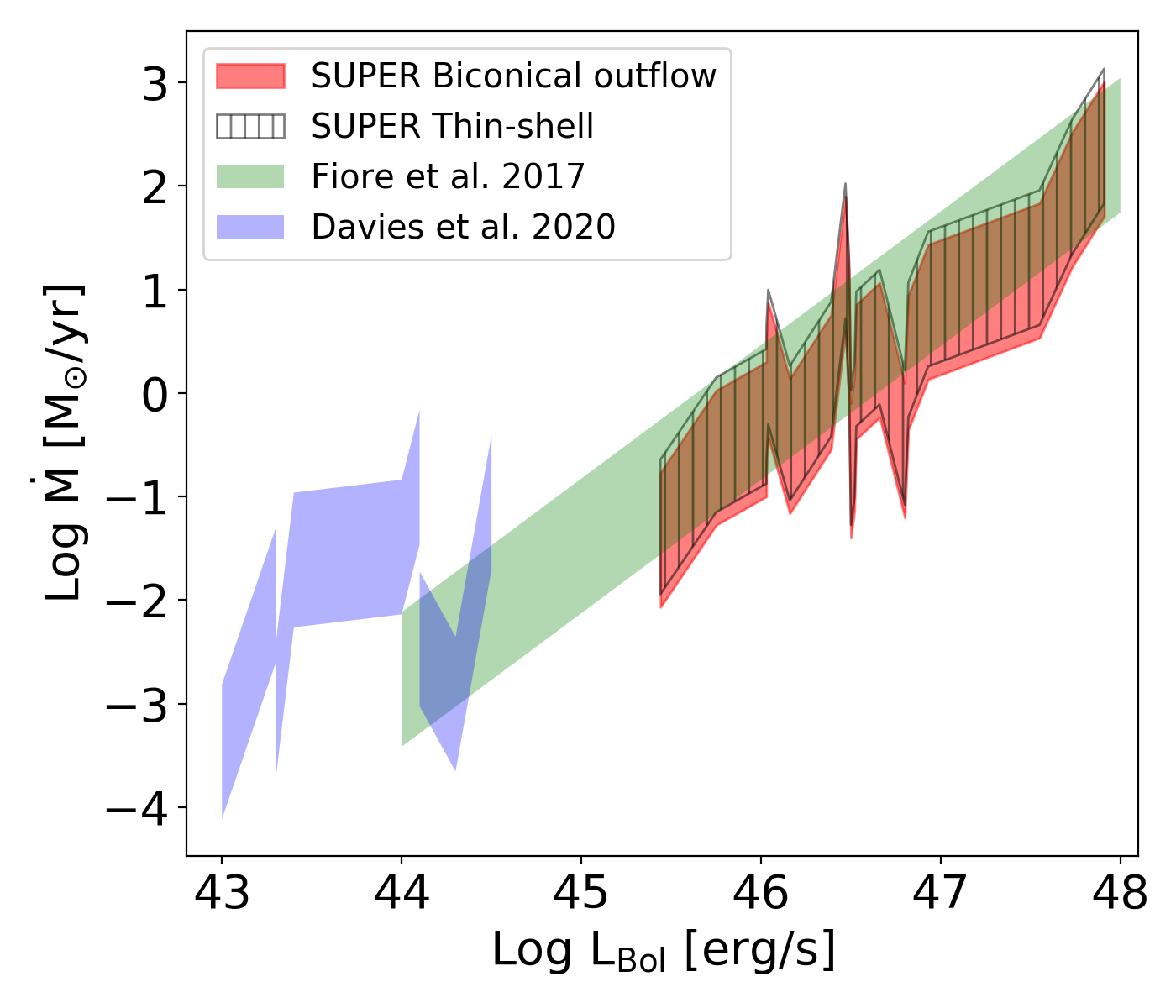
Figure 11: Ionized gas [O iii] mass outflow rate vs. the bolometric luminosity of the AGN for SUPER Type-1 sample presented in this paper and literature data of low as well as high redshift AGN. The red shaded area and the black hatched area shows the mass outflow rates for the SUPER targets assuming a bi-conical outflow model and a thin-shell model, as described in Sect. 5.5. The green shaded area shows the outflow rates for ionized gas from literature data compiled in Fiore et al. (2017) (after rescaling the relation with the same assumption as the Type-1 SUPER targets, see Sect. 5.5) and the blue shaded region shows the outflow rates for low redshift X-ray AGN sample from Davies et al. (2020a). The shaded region in all the studies correspond to mass outflow rates assuming an electron density from 500 cm^-3 – 10,000 cm^-3.

There are a couple of targets with notably interesting features from the spectroastrometry analysis. In the case of cid_346, the spectroastrometry method reveals the presence of gas moving at $\sim$600 km/s at a distance of $\sim$0.3^′′ equivalent to a physical distance of $\sim$4 kpc from the AGN location. Similarly, also in the case of S82X1905 we find that the bulk of the gas moving at $\sim 300$ km/s is located at $\sim$4 kpc from the center. We argue that a possible explanation for such extended redshifted emission is that the receding part of the outflow is not obscured by the dust of the host galaxy in these two cases, possibly due to the larger extent of the outflow itself.

We also note from the spectroastrometry maps that the bulk of the low velocity [O iii] component i.e. the non-outflowing component of the [O iii] emission is not necessarily emitted at the same location as that of the AGN in a few targets. This is expected as even in low redshift galaxies the [O iii] emission is dominated in the extended NLR in the form of ionization cones, which are not co-spatial with the AGN location.

We now summarize the different methods used to determine the extension of the ionized gas and the outflows associated with the gas. Using COG and PSF-subtraction methods, we compared the spatial distribution of the ionized gas with the observed PSF and inferred whether the ionized gas is extended or not. The COG and PSF-subtraction methods rely on robust PSF measurements either from the BLR emission or if the BLR emission is not available, a dedicated PSF observation. Using either of these methods, we find that the ionized gas is extended in X_N_81_44, X_N_66_23, X_N_115_23, cid_346, J1333+1649, J1549+1245 and S82X1905. In these targets with extended ionized gas, we constructed the flux and velocity maps and calculated $\mathrm{D_{600}}$ value which is the maximum projected spatial extent of $\mathrm{w_{80}}$ ¿ 600 km/s. The $\mathrm{D_{600}}$ parameter quantifies the spatial extent of the outflow associated with the ionized gas which is consistent with the outflow definition we have adopted throughout this paper i.e. $\mathrm{w_{80}}$ ¿ 600 km/s. The $\mathrm{D_{600}}$ parameter is in the range $\approx$1.5–6.5 kpc from the AGN location. The $\mathrm{D_{600}}$ parameter should only be determined for targets which show the presence of extended ionized gas emission beyond the observed PSF. Lastly, we determined the radial distance at which the bulk of the ionized gas (weighted by luminosity) is moving at velocity greater than 600 km/s using spectroastrometry technique. We find that for most galaxies the bulk of the high velocity gas (—v—¿600 km/s) is contained within $\sim$1 kpc from the AGN location. The spectroastrometry technique has the advantage that it can be used for targets which are unresolved or marginally resolved. However, the technique does not provide the true spatial extent of the ionized gas, but the centroid of the bulk gas moving at a specific velocity.

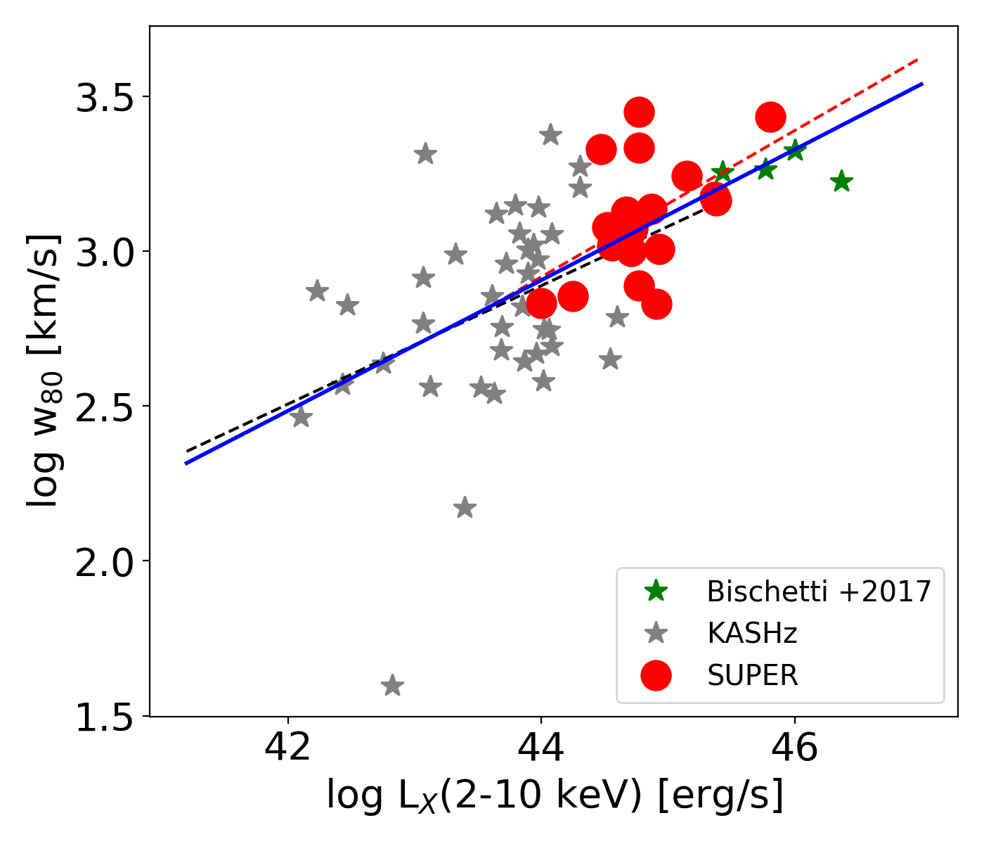
(a)

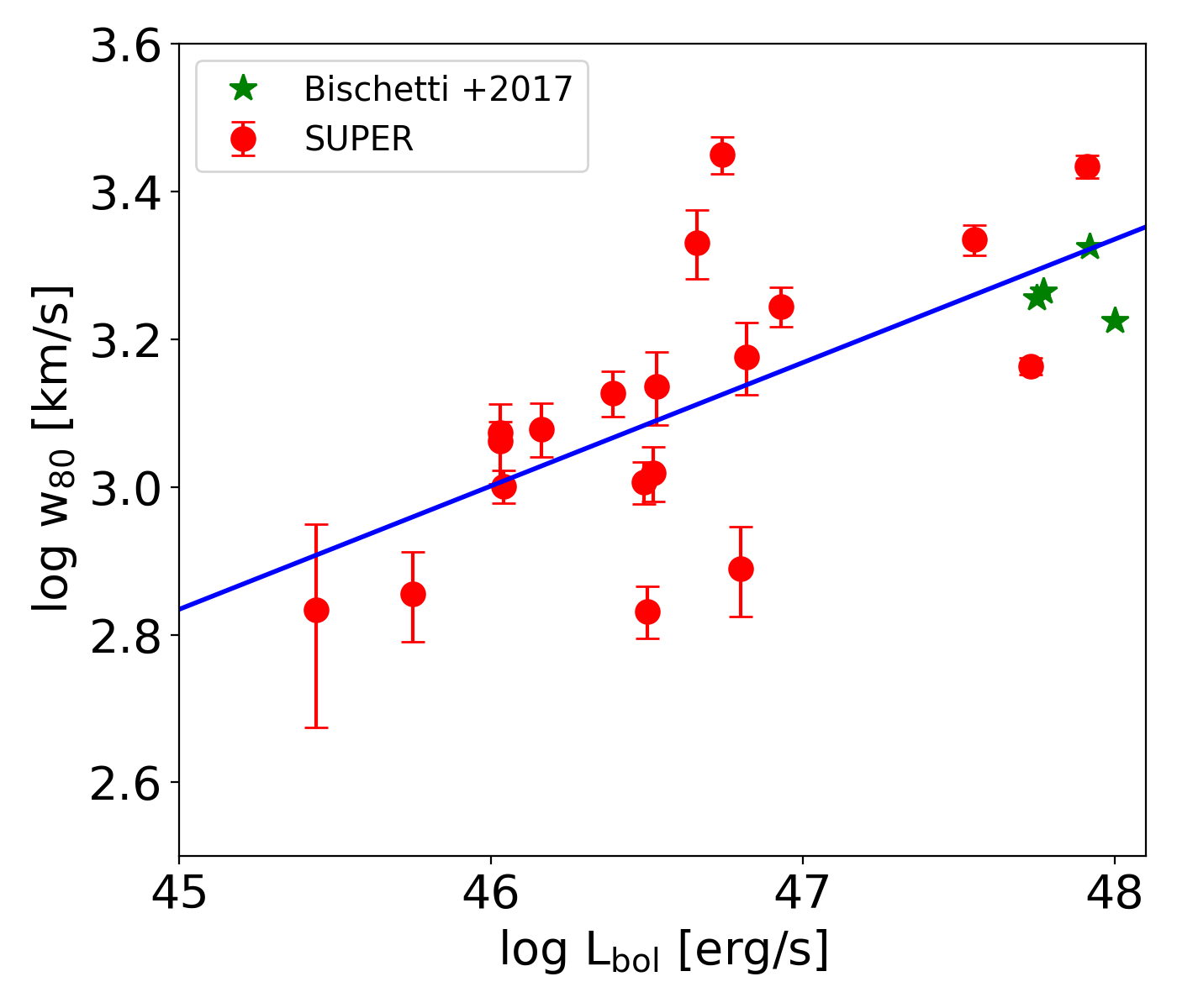
(b)

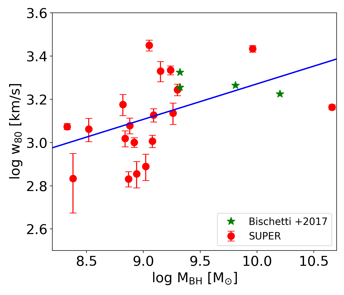
(c)

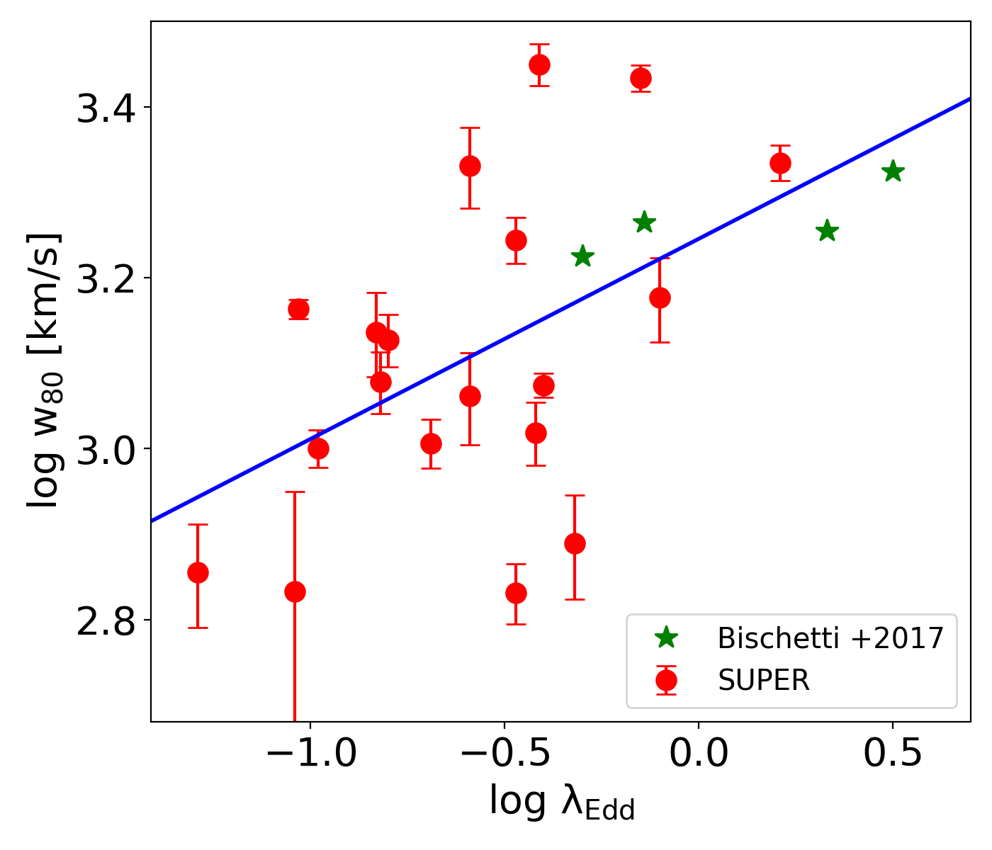
(d)

Figure 12: Top left panel: Non-parametric velocity width, $\mathrm{w_{80}}$ derived from the integrated spectrum vs. X-ray luminosity measured in the 2-10 keV band. The red data points represent the SUPER sample, the grey data points show the luminosity and redshift-matched sample from the KASHz survey and the green data points show the high luminosity sample from WISSH survey. The dashed red line shows the best fit relation for SUPER galaxies, the dashed grey line shows the best fit relation for matched KASHz sample and the blue line shows the overall relation for SUPER, KASHz and the WISSH sample (Bischetti et al., 2017). Top right panel: $\mathrm{w_{80}}$ vs. bolometric luminosity. Bottom left panel: $\mathrm{w_{80}}$ vs. black hole mass, $\mathrm{M_{BH}}$. Bottom right panel: $\mathrm{w_{80}}$ vs. Eddington ratio ($\mathrm{L_{bol}/L_{Edd}}$). In all the plots, the blue line shows the best fit to all the data points within the plot. The values plotted for the SUPER sample are obtained from Tables 1 and 3.

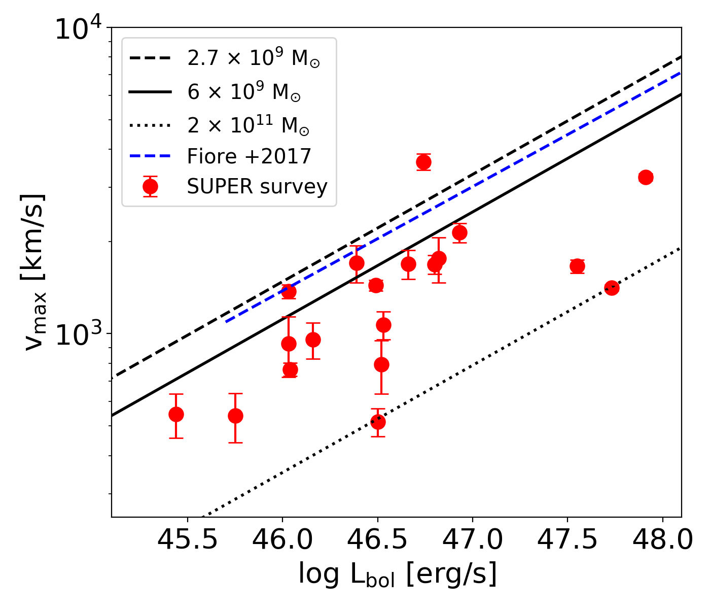
(a)

Figure 13: Maximum velocity, $\mathrm{v_{max}}$, defined in Sect. 6, vs. AGN bolometric luminosity. The red circles represent the SUPER targets, the dashed blue line shows the best-fit relation for literature data compiled in Fiore et al. (2017). The black curves are the Menci et al. (2019) predictions for the shock velocity (approximated here by the measured v_max) vs. AGN luminosity for galaxies. The three curves correspond to molecular gas masses of 2.7 $\times 10^{9}$ M_⊙, 6 $\times 10^{9}$ M_⊙ and 2 $\times 10^{11}$ M_⊙ respectively. More details are given in Sect. 6.

5.5 Mass outflow rates

To understand the impact that AGN feedback may have on their host galaxies it is important to estimate the mass of the ouflowing gas and the kinetic energy associated with it. Although the ionized gas phase is believed to trace only a fraction of the total outflow mass (e.g. Cicone et al., 2018), the energy associated with these outflows can provide valuable information on its driving mechanism (e.g. Fiore et al., 2017; Brusa et al., 2018; Husemann et al., 2019; Shimizu et al., 2019).

An accurate estimation of the mass outflow rate for high redshift galaxies is a major challenge due to the limited spatial resolution achievable with current instrumentation and the uncertainties on the physical properties of the outflowing gas. As a consequence, there is the need to make a number of assumptions which leads to large uncertainties in the derived mass outflow rate. The key elements that need to be constrained to estimate the mass outflow rate are: the geometry and the volume of the outflow; the physical properties of the gas (e.g. its electron density, temperature and associated metallicity); the velocity of the outflowing gas and its radial evolution. For the scope of this paper, we focus on reporting the range of mass outflow rates derived from our measured quantities by exploring the possible assumptions for key physical quantities, described as follows.

Geometry: Both theoretical models (e.g. Ishibashi et al., 2019) and results from imaging and IFU observations of low redshift galaxies (e.g. Crenshaw et al., 2010; Müller-Sánchez et al., 2011; Liu et al., 2013; Wylezalek et al., 2016; Venturi et al., 2018) provide evidence for the presence of spherical and conical outflow morphology. Recent observations of low redshift AGN host galaxies have also suggested the possibility of expanding shell-like shocks driving an outflow across the host galaxy (e.g. Husemann et al., 2019). A shell-like expanding outflow model can take into account variable physical quantities such as the outflow luminosity, velocity, density and temperature as a function of distance from the AGN. Total outflow rate throughout the galaxy is then the sum over all the shells. As current observations with SINFONI do not allow us to infer the outflow morphology, we will calculate mass outflow rates assuming both bi-conical and thin shell geometry. A spherical geometry would change the overall normalization factor in the mass outflow rate formula but not the general trends, when compared with the bi-conical outflow geometry. We will consider the volume up to a distance of 2 kpc from the AGN (see further discussion on ”Radius and Velocity” later in the section). For the thin-shell model, we will assume a shell width of $\sim$500 pc which is the upper end of the limits inferred in low redshift AGN host galaxies (e.g. Husemann et al., 2019).

Luminosity: For an emission line modeled using multiple Gaussian components, the broad Gaussian component is often associated with the outflowing gas. However, as stated in earlier sections, the detection of an additional broad component depends on the S/N of the data and the model function used. Therefore, we will continue to use the non-parametric approach and define the outflow luminosity as the luminosity calculated from the flux of the [O iii] $\lambda$5007 emission line channels at —v—¿300 km/s. This definition is consistent with our outflow’s classification, i.e. $\mathrm{w_{80}}$ ¿ 600 km/s, presented in Sec. 5.1. The outflow luminosity as defined above is reported in Table 4. We note that the average ratio between the broad component luminosity (Table 1) and the outflow luminosity ranges from 0.56–4.07 with a mean ratio of 1.80$\pm$0.89. Therefore, on average the luminosity of the broad Gaussian component is higher than that estimated from the non-parametric procedure described above. We finally note that the luminosity calculated in this paper is not corrected for extinction and therefore represents a lower limit on the outflow luminosity.

Radius and velocity: Several spatially resolved observations of ionized gas at low redshift clearly show a radial dependence of outflow properties (e.g. Kakkad et al., 2018; Venturi et al., 2018; Husemann et al., 2019). It is therefore necessary to take into account the variations in the velocity across the outflowing medium while calculating the mass outflow rates. Due to the relatively low spatial resolution of high redshift targets compared to the low redshift AGN, deriving spatial variations in the physical properties of the outflow is not always feasible. Observations at low redshift report outflow radius values up to few kiloparsecs (e.g. Liu et al., 2013; Husemann et al., 2016). For the purpose of this paper, we will calculate the mass outflow rate up to a fixed radius of $\sim$2 kpc, which is also the maximum radius for unresolved targets (see PSF values in Table 2). The outflow velocity at 2 kpc will be derived from the $\mathrm{w_{80}}$ maps in case of resolved targets (Figs. 7 and 8) and the integrated $\mathrm{w_{80}}$ value in case of unresolved targets. Other definitions for outflow velocity have also been used in the literature such as broad Gaussian widths and $\mathrm{v_{max}}$, which can introduce a systematic uncertainty up to a factor of $\sim$2 in the calculation of mass outflow rate (e.g. Kakkad et al., 2016; Fiore et al., 2017).

Density: The electron density represents the major source of uncertainty in the calculation of mass outflow rates (e.g. Harrison et al., 2018) since it is very challenging to measure it and in fact there is a wide range of values reported in the literature for the gas density in the NLR (Perna et al., 2017; Kakkad et al., 2018; Baron & Netzer, 2019; Davies et al., 2020a). Similarly to the outflow’s velocity, variations in the electron density across the outflowing medium make the calculation of outflow rates even more challenging. Moreover, key diagnostic emission lines to estimate electron density such as [S ii] $\lambda$6716, 6731 are too faint or remain undetected for the SUPER targets. Therefore, instead of assuming a single value for the gas density, we will consider two values that cover the wide range observed in the literature, i.e. from 500 cm^-3 – 10,000 cm^-3, which would return maximum and minimum possible outflow rates given the rest of the model assumptions described above.

Since H$\beta$ is relatively faint, we will calculate the mass of the outflowing ionized gas from the [O iii] $\lambda$5007 line as follows (see e.g. Carniani et al., 2015; Kakkad et al., 2016):

$$\mathrm{M_{[{O\textsc{iii}}]\leavevmode\nobreak\ }^{out}=0.8\cdot 10^{8}M_{\odot}\left(\frac{1}{10^{[O/H]-[O/H]_{\odot}}}\right)\left(\frac{L_{[{O\textsc{iii}}]\leavevmode\nobreak\ }}{10^{44}\leavevmode\nobreak\ erg/s}\right)\left(\frac{<n_{e}>}{500cm^{-3}}\right)^{-1}}$$ (1)

where all the oxygen is assumed to be ionized to O²⁺, the electron temperature is 10,000 K and [O/H], the metallicity of the outflowing material, is assumed solar. For a uniformly filled bi-conical outflow, the mass outflow rate takes the form (Fiore et al., 2017):

$$\mathrm{\dot{M}_{[{O\textsc{iii}}]\leavevmode\nobreak\ ,cone}^{out}=3\cdot v_{out}\frac{M_{out}}{R_{out}}}$$ (2)

where $\mathrm{v_{out}}$ is the outflow velocity, $\mathrm{M_{out}}$ is obtained from Eq. 1 and $\mathrm{R_{out}}$ is the distance at which the outflow rate is computed. We are making the assumption here that the bi-conical outflow region is uniformly filled with ionized gas with density ¡$\mathrm{n_{e}}$¿. Eq. 2 will give the instantaneous outflow rate of the ionized gas crossing the spherical sector at distance $\mathrm{R_{out}}$ from the AGN. On the other hand, if the outflow is assumed to propagate in thin-shells of thickness $\mathrm{\Delta R}$ (assumed 500 pc here) which shock against the ISM, the outflow rate is simply (Husemann et al., 2019):

$$\mathrm{\dot{M}_{[{O\textsc{iii}}]\leavevmode\nobreak\ ,thin-shell}^{out}=v_{out}\frac{M_{out}}{\Delta R}}$$ (3)

where $\mathrm{v_{out}}$ is the outflow velocity at the location of the shell (assumed to be at 2 kpc here). Eq. 3 will provide the outflow rate within the shell of thickness $\mathrm{\Delta R}$ instead of an integrated value.

We compute the mass outflow rates using both formulas described above and for two values of the electron density: 500 cm^-3 and 10⁴ cm^-3 (e.g. Baron & Netzer, 2019; Davies et al., 2020a). The values obtained are reported in Table 4. Note that most of the SUPER targets have mass outflow rate values below 10 $\mathrm{M_{\odot}}$/yr for the density range 500 cm^-3 to 10⁴ cm^-3. At the high luminosity end, however, the mass outflow rate values exceed 10 $\mathrm{M_{\odot}}$/yr even for a conservative electron density value of 10⁴ cm^-3. In Fig. 11 we show the range of mass outflow rates vs. the bolometric luminosities covered by our sample, from literature ionized gas outflow rates compiled in Fiore et al. (2017), and from the low-redshift X-ray AGN studied in Davies et al. (2020a). The mass outflow rates values from Fiore et al. (2017) and Davies et al. (2020a) have been updated to match the electron density range used in this study. In addition, these literature mass outflow rates from Fiore et al. (2017) and Davies et al. (2020a) have also been re-scaled to match the methodology used in this paper. Fiore et al. (2017) used the luminosity of the broad Gaussian component as a proxy for the outflow luminosity, while, as described above, we considered only channels with —v—¿300 km/s. We verified that for our objects the mean ratio between the luminosity calculated from the broad Gaussian and the luminosity from [O iii] channels at —v—¿300 km/s is $\approx$2 and re-scaled by this factor the values from Fiore et al. (2017). A similar scaling was used for Davies et al. (2020a) who use the [O iii] luminosity to calculate the outflow mass. The $\mathrm{\dot{M_{out}}-L_{bol}}$ relation in Fiore et al. (2017) also used, when available, either $\mathrm{H\alpha}\leavevmode\nobreak\$ or $\mathrm{H\beta}\leavevmode\nobreak\$ to calculate the total mass outflow rates for the ionized gas. Outflow rates for sources with only [O iii] detection were scaled by a factor of three which was consistent with the mean ratio between the $\mathrm{H\alpha}\leavevmode\nobreak\$ and [O iii] luminosities in their sample. We have therefore applied the same factor to their relation to make it consistent with us using the [O iii] luminosities. After taking these factors into account, the Fiore et al. (2017) relation roughly match the mass outflow rates observed for the Type-1 sample in this paper. Fig. 11 clearly illustrates that the different assumptions on the outflow geometry (i.e. by-conical outflow or thin spherical shell) have, by far, a smaller impact on the derived value for the mass outflow rate than the assumed value of the gas density. The latter is responsible for more than an order of magnitude difference in the range on n_e explored. Finally, combining the SUPER Type-1 sample presented in this paper with literature data we confirm a correlation of the mass outflow rate with the AGN bolometric luminosity across five orders of magnitude. This relation could be potentially used to put constraints on the different AGN outflow models, but we caution that the real scatter and the slope of this relation is uncertain as long as we do not have better constraints on the gas density object by objects (see also Davies et al. (2020a)).

Finally, as argued in Baron & Netzer (2019), the ionized gas is most likely associated with a significant amount of neutral dusty gas that takes part in the same outflow. Along with the fact that outflows can exist in multiple gas phases (e.g. Perna et al., 2019; Serafinelli et al., 2019), this suggests that the actual mass outflow rates can be substantially larger than the ones deduced here.

6 Scaling Relations

We now focus on the relation between the properties of the detected outflows (e.g. velocity and escape fraction) and the properties of the central super-massive black (e.g. bolometric luminosity and black hole mass). Theoretical models of AGN outflows predict fast winds to originate from the accretion disk which later impact on the ISM resulting in a forward shock that expand within the host galaxy (e.g. Zubovas & King, 2012; Zubovas & Nayakshin, 2014; Faucher-Giguère & Quataert, 2012; Wagner et al., 2013). This would naturally predict positive correlations between outflow properties (e.g. velocity, mass outflow rate) and AGN properties (e.g. King & Pounds, 2015). The slope of such relation will in addition depends on the density profile of the medium (e.g. Faucher-Giguère & Quataert, 2012). While there are already a few studies exploring such scaling relations for literature samples of AGN on a wide redshift range (e.g. Fiore et al., 2017; Fluetsch et al., 2019), we will perform a similar analysis on the SUPER sample for which we have a homogeneous and detailed characterization of both the outflows properties as well as those of the central black hole.

Table 5: Correlation functions and statistical parameters for the scaling relations in Fig. 12.

Correlation	Slope	Pearson coefficient	$p$-value
$\mathrm{w_{80}}$ vs. $\mathrm{L_{X}}$ †	0.21$\pm$0.01	0.59	¡1.0e-5
$\mathrm{w_{80}}$ vs. $\mathrm{L_{X}}$ ∗	0.21$\pm$0.01	0.51	0.024
$\mathrm{w_{80}}$ vs. $\mathrm{L_{bol}}$ ∗∗	0.16$\pm$0.04	0.70	2.1e-4
$\mathrm{w_{80}}$ vs. $\mathrm{M_{BH}}$ ∗∗	0.16$\pm$0.06	0.50	0.02
$\mathrm{w_{80}}$ vs. $\mathrm{\lambda_{edd}}$ ∗∗	0.23$\pm$0.07	0.57	4.0e-3
$\mathrm{f_{esc}}$ vs. $\mathrm{L_{bol}}$ ∗∗	23.5$\pm$6.7	0.65	0.003

Notes:
^†The values reported for the $\mathrm{w_{80}}$ vs. $\mathrm{L_{X}}$ relation are for the SUPER, KASHz and Bischetti et al. (2017) targets combined. ^∗The reported values for the $\mathrm{w_{80}}$ vs. $\mathrm{L_{X}}$ relation consider the SUPER sample. ^∗∗The reported values for the $\mathrm{w_{80}}$ vs. $\mathrm{L_{X}}$ relation consider the SUPER and Bischetti et al. (2017) sample.

We first investigate the scaling relations for $\mathrm{w_{80}}$ (Fig. 12) versus the physical properties of the central SMBH. In the top left panel of Fig. 12, we plot $\mathrm{w_{80}}$ against the AGN X-ray luminosity $\mathrm{L_{X}(2-10keV)}$. A clear positive trend is present i.e. higher X-ray luminosity targets show larger [O iii] width. A similar positive correlation is observed if we consider the AGN bolometric luminosity (top right panel in Fig. 12) instead of the X-ray luminosity. To cover a wider range in luminosity, we add the AGN sample observed in the KASHz survey matched in redshift (z$\sim$2–2.5) and the high luminosity targets from the WISSH survey (e.g. Bischetti et al., 2017; Martocchia et al., 2017; Zappacosta et al., 2020). We derived the Pearson coefficient and the p-value for each of these relations and the results are reported in Table 5. For the SUPER data alone, the Pearson coefficient for $\mathrm{w_{80}}$ vs. $\mathrm{L_{X}}$ relation is 0.51 while for the redshift matched KASHz sample the coefficient is 0.37 with a null hypothesis probability (for a non-correlation) of $\sim$2.4% and 2% respectively. For the combined datasets of SUPER, KASHz and WISSH sample, the Pearson coefficient and the null hypothesis probability is 0.59 and ¡0.001% respectively, suggesting a strong correlation between $\mathrm{w_{80}}$ and $\mathrm{L_{X}}$.

The statistical tests also confirm strong positive correlation for $\mathrm{w_{80}}$ vs. $\mathrm{L_{bol}}$ (Fig. 12, null-hypothesis probability ¡0.1%), which may be interpreted as an increase in the turbulence of the gas within the AGN host galaxies with the overall radiation power of the central black hole. We note that there is a positive correlation also for $\mathrm{v_{10}}$ vs. $\mathrm{L_{X}}$ and $\mathrm{L_{bol}}$, although they are weaker, according to the Pearson test, compared to those presented above for $\mathrm{w_{80}}$.

Further exploring the correlation of the gas kinematics with the AGN properties, $\mathrm{w_{80}}$ has a relatively weak correlation with the black hole mass (bottom left panel in Fig. 12) with a null hypothesis of $\sim$2%. Similar correlation is observed between $\mathrm{w_{80}}$ and the Eddington ratio ($\mathrm{\lambda_{Edd}=L_{bol}/L_{Edd}}$, where $\mathrm{L_{Edd}=1.3\times 10^{38}(M_{BH}/M_{\odot}}$ erg/s)) with a null-hypothesis probability of $\sim$0.4%. These values suggest that the outflow velocity correlate weakly with the black hole mass when compared with the correlation with bolometric luminosity.

Apart from $\mathrm{w_{80}}$, we tested the presence of a correlation in the $\mathrm{L_{bol}}$ vs. maximum velocity of the [O iii] line (Fig. 13), defined in the literature as $\mathrm{v_{max}=\Delta\lambda_{broad}+2\sigma_{broad}}$ i.e. the sum of the difference between the centroid velocity of the broad and the narrow component and twice the velocity dispersion of the broad component (e.g. Rupke & Veilleux, 2013). The Pearson coefficient for the relation between $\mathrm{v_{max}}$ and $\mathrm{L_{bol}}$ is 0.68 with a null hypothesis probability of 0.1%, confirming also in this case a positive correlation between these two quantities. Note that despite the similar proportionality, the normalization of the curve in the SUPER sample and that in the Fiore et al. (2017) sample are different. We expect that the velocity of the outflowing gas depends on the properties of the medium it is moving through, which would result in some intrinsic scatter in any correlation between such velocity and the AGN bolometric luminosity. The difference in the normalization can also stem from differences in the gas mass of the host galaxies as explained below.

To test the latter hypothesis we consider the Menci et al. (2019) model which provides a two-dimensional description of the expansion of an AGN-driven shock in a disk with an exponential gas density profile. Their predictions are expressed in terms of the total molecular gas mass and circular velocity of the host galaxy. In particular, from Eq. 14 in Menci et al. (2019), we can express the velocity of the shock, $\mathrm{V_{S}}$, as a function of the AGN bolometric luminosity, $\mathrm{L_{bol}}$ and host galaxy gas mass, $\mathrm{M_{gas}}$, in the following way:

$$\mathrm{log\Bigg{(}\mathrm{\frac{V_{S}}{km/s}}\Bigg{)}=2.65+0.35\,log\Bigg{(}\frac{L_{bol}}{10^{45}\leavevmode\nobreak\ ergs^{-1}}\Bigg{)}-\frac{1}{3}log\Bigg{(}\frac{M_{gas}}{10^{10}\leavevmode\nobreak\ M_{\odot}}\Bigg{)}}+\\ \mathrm{log\Bigg{(}\frac{V_{c}}{200\leavevmode\nobreak\ km/s}\Bigg{)}-0.65\,log\Bigg{(}\frac{R_{S}}{1\leavevmode\nobreak\ kpc}\Bigg{)}}$$ (4)

(a)

Figure 14: The plot shows the escape fraction as a function of the bolometric luminosity of the AGN for the Type-1 sample presented in this paper. The escape velocity is calculated for a distance of 2 kpc from Eq. 5. The blue curve shows the best-fit relation.

We use the above formula to predict the scaling of the outflow velocity versus the AGN bolometric luminosity for a range of host galaxies properties that encompass, to the best of our knowledge, those of our sample. We assume that the circular velocity ($\mathrm{V_{c}}$) of the galaxy is $\approx$300 km/s which is a reasonable assumption from the Tully-Fischer relation for galaxies with M${}_{\ast}\approx 10^{9}-10^{11}{\rm M}_{\odot}$ (e.g. Cresci et al., 2009). We fix the radius of the shock (R_S) to $\approx 1$kpc which is where the bulk of the outflowing gas is located following our spectroastrometry analysis in Sect. 5.4. We use our CO(3-2) ALMA follow-up observations (Circosta et al. in prep.) to estimate the range of molecular gas masses for our AGN hosts: the mean gas mass for the sample is M${}_{\rm gas}\approx 6\times 10^{9}$ M_⊙, with 90$\%$ of the sample above M${}_{\rm gas}\approx$ 2.7$\times 10^{9}$ M_⊙ and maximum measured gas mass is M${}_{\rm gas}\approx 2\times 10^{11}$M_⊙. As it can be seen in Fig. 13 the range of model tracks (shown by the black relations) is able to reproduce most of our observed values (shown as red circles), where we have assumed that $\mathrm{v_{max}}$ is a good approximation of V_S. Therefore the Menci et al. (2019) description of an AGN-driven shock moving through a galaxy disk is able to reproduce our observations once the observed range of molecular gas masses for the host galaxies is used. The data points lying outside the model predictions from Menci et al. (2019) can be explained if galaxies with lower or higher molecular gas mass are taken into account.

AGN-driven outflows are suggested as a physical mechanism able to effectively remove gas from their host galaxies, which is a very important process to reproduce the observed mass build-up of galaxies in the local universe and the chemical composition of the ISM (e.g. Muratov et al., 2015). We can use the [O iii] velocity profile to estimate the fraction of the ionized gas which has the ability to escape the gravitational potential of AGN host galaxy. We first calculate the escape velocity of a cloud which is at a distance r from the AGN location (see Rupke et al., 2002):

$$\mathrm{V_{esc}=\sqrt{2}V_{c}\left[1+ln\left(\frac{r_{max}}{r}\right)\right]^{1/2}},$$ (5)

where $\mathrm{r_{max}}$ is the extent of the dark matter halo (assumed $\sim$100 kpc here) and $\mathrm{V_{c}}$ is the circular velocity of the galaxy, assumed 300 km/s as Eq. 4 from the Tully-Fischer relation for the range of stellar mass in SUPER galaxies (see Cresci et al., 2009). At 2 kpc, which is roughly the spatial resolution of the H-band SINFONI observations, the escape velocity calculated using Eq. 5 is on average $\sim$950 km/s. We then estimate the escape fraction of ionized gas as the ratio between the flux of the [O iii] $\lambda$5007 channels in the integrated spectra with —v— ¿ $\mathrm{V_{esc}}$ and the total flux of the [O iii] $\lambda$5007 line. The escape fraction of the ionized gas calculated for the Type-1 SUPER sample presented in this paper is reported in Table 4. For most galaxies, $\lesssim$10% of the outflowing ionized gas has the ability to escape the host galaxy, while the rest of the gas is expected to re-accrete back onto the host galaxy. The highest escape fractions of $\sim$43% and $\sim$97% are observed in J1333+1649 and J1441+0454 which are also the targets with high bolometric luminosity. Note that in J1441+0454, the exceptional high escape fraction is a result of the extremely blue-shifted [O iii] profile which is also blended with the iron emission as explained in Sect. 5.1. Fig. 14 shows the escape fraction as a function of the bolometric luminosity which suggests a positive correlation between the two quantities, but with a large scatter. The Pearson correlation coefficient between the escape fraction and the bolometric luminosity is 0.64 with a null hypothesis probability of $\sim$0.2%. Although the correlation is relatively weak compared to the $\mathrm{w_{80}}-L_{bol}$ relation in Fig. 12, the data might suggest that outflows hosted in high luminosity AGN have a higher fraction of escaping gas.

We also note that SINFONI data only trace the ionized phase of the outflow, while a large fraction of the outflow might be present in the molecular gas phase (e.g. Cicone et al., 2018; Fluetsch et al., 2019). Therefore, follow-up studies in other gas phases such as the warm and cold molecular phase and neutral gas phase are required to complete the picture of the effects of radiation pressure on the ISM of the galaxies.

7 Summary and Conclusions

We present near-infrared IFU spectroscopy for 21 X-ray selected Type-1 AGN from the SUPER survey (half of the survey size). We trace and characterize the velocity and extension of the ionized gas, and its outflow component, in the Narrow Line Region using the [O iii] $\lambda$5007 transition. The main conclusions from the work presented in this paper are summarized below.

• Using a cut on the non-parametric velocity width, $\mathrm{w_{80}}>600$ km/s, in the integrated spectra, we find that all the Type-1 AGN in the SUPER survey show the presence of ionized outflows. We consider the selected threshold in $\mathrm{w_{80}}$ a conservative choice, based on the very diverse distributions of low-z and high-z mass matched sample of start forming galaxies compared to the $\mathrm{w_{80}}$ distribution of AGN host galaxies (Sect. 5.1, Fig. 3). We also confirm a strong linear correlation between the [O iii] luminosity and the X-ray luminosity, as previously observed in the literature (Sect. 5.1, Fig. 4).

• Using three different methods (curve of growth analysis, half-light radii and PSF-subtraction method) we find evidence of kiloparsec-scale extended ionized gas emission in seven out of the eleven targets for which [O iii] is detected at a S/N$>5$ in the integrated spectrum (Sect. 5.2, Figs. 5 and 6). Flux and velocity maps of these resolved targets reveal outflows extended to $\sim 6$ kiloparsec (quantified by $\mathrm{D_{600}}$ value, Table 4 and Figs. 7 & 8), with indications of redshifted outflows in three objects (cid$\_346$, J1333+1649 and S82X1905).

• We use the spectroastrometry method to determine the distance of the bulk of the gas moving at a given velocity. We find that the high velocity outflowing gas (—v— ¿ 600 km/s) is contained in the central $\sim$1 kpc for $\sim$80% of the targets for which the spectroastrometry analysis was performed (Sect. 5.4). For two objects (cid_346 and S82X1905) the bulk motion of high velocity gas is extended to $\sim$3 kpc.

• We explore a range of plausible assumptions on the physical properties of the outflow (its geometry, velocity and radius) and of the outflowing gas (i.e. its electron density) and report the range of derived mass outflow rates for each target (Sect. 5.5). The mass outflow rates of the Type-1 sample are in the range $\sim$0.01–1000 $\mathrm{M_{\odot}}$/yr (Table 4). After factoring in the systematic uncertainties in the outflow models, these outflow rates seem to correlate with the bolometric luminosity of the AGN.

• The non-parametric velocity, $\mathrm{w_{80}}$, strongly correlates with the X-ray luminosity, $\mathrm{L_{X}(2-10keV)}$, and the bolometric luminosity of the central super-massive black hole (Fig. 12). The correlation is relatively weak for $\mathrm{w_{80}}$ vs. $\mathrm{M_{BH}}$ (or $\mathrm{L_{Edd}}$). The maximum velocity vs. bolometric luminosity plot for the SUPER sample agree with model predictions for an AGN-driven shock driving an outflow through a galaxy disk (Fig. 13).

• For most galaxies, ¡10% of the outflows in the ionized gas have the potenial to escape the gravitational potential of the host galaxy. The escape fraction also increases with the bolometric luminosity of the AGN (Fig. 14).

While this paper focused on presenting the ionized gas kinematics of the Type-1 sample, an upcoming publication will present the SINFONI and ALMA results for the overall (Type-1 and Type-2) AGN SUPER sample. The different types of morphology of the ionized gas and the associated outflows presented in this paper clearly show the advantages of performing high spatial resolution observations. Even better spatial and spectral resolution and higher sensitivity is expected with future facilities such as ELT/HARMONI. Such observations will enable us to resolve the extended redshifted and blueshifted outflowing gas which might reveal sub-structures within the outflow, and trace the radial evolution of the outflowing gas, which is certainly not possible at z$\sim 2$ with today’s instrumentation. Finally, we are currently limited to study ionized outflows from the ground up to z$\approx 4$, observing the [O iii] line in the K-band. With the IFU capabilities of NIRSpec on-board of JWST, a study similar to the one presented in this paper could be performed with comparable resolution at z$>4$ and will allow to further constrain the importance of AGN feedback at earlier comic epochs.

Acknowledgements: We thank the referee for the useful and constructive comments. We thank Michele Cirasuolo, Alice Concas and Dominika Wylezalek for providing the comparison data for the $\mathrm{w_{80}}$ distribution. MP is supported by the Programa Atracción de Talento de la Comunidad de Madrid via grant 2018-T2/TIC-11715. Based on observations collected at the European organisation for Astronomical Research in the Southern Hemisphere under ESO program 196.A-0377.

Appendix A Integrated H-band Spectra and [O iii] channel maps of Type-1 SUPER sample

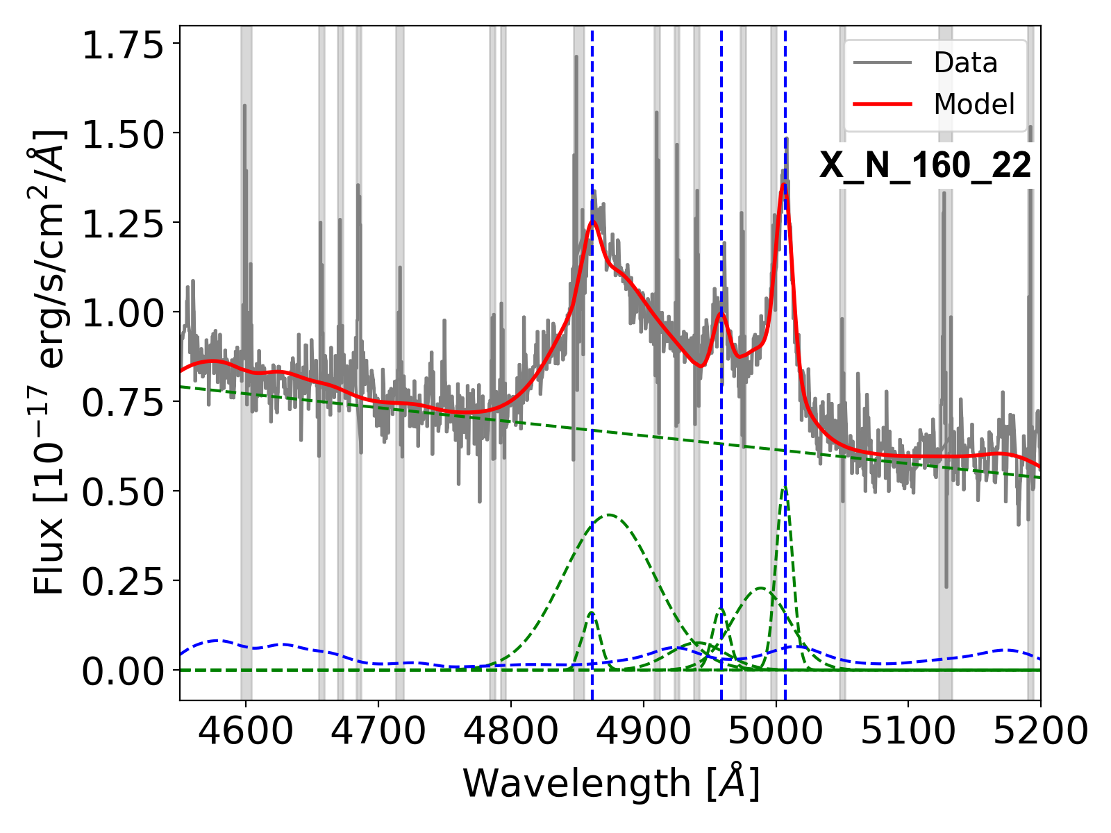
(a)

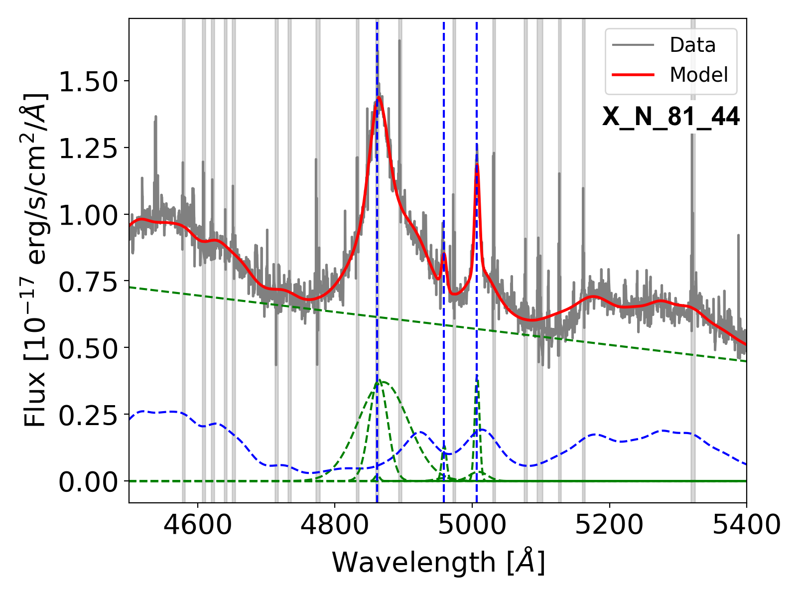
(b)

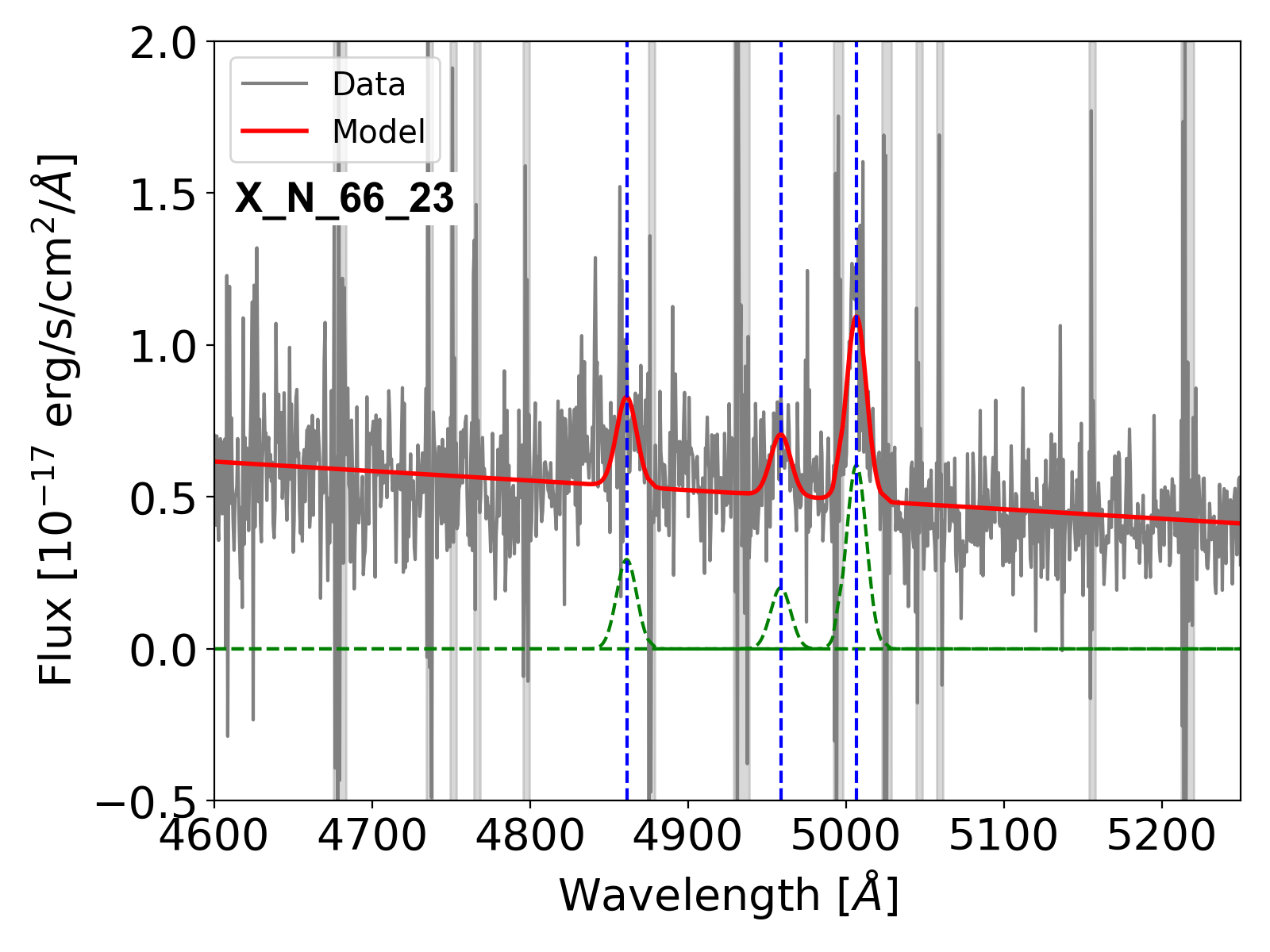
(c)

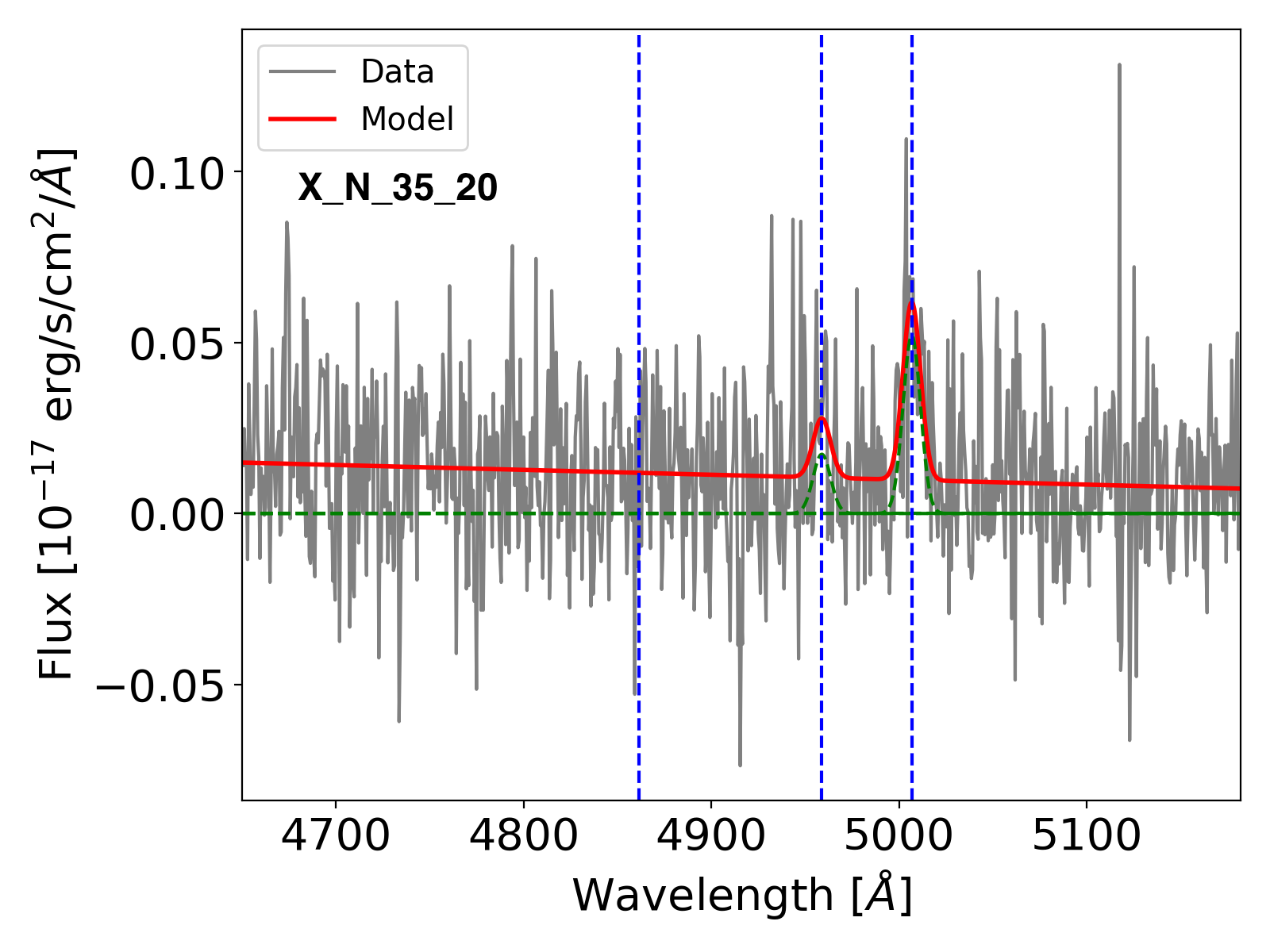
(d)

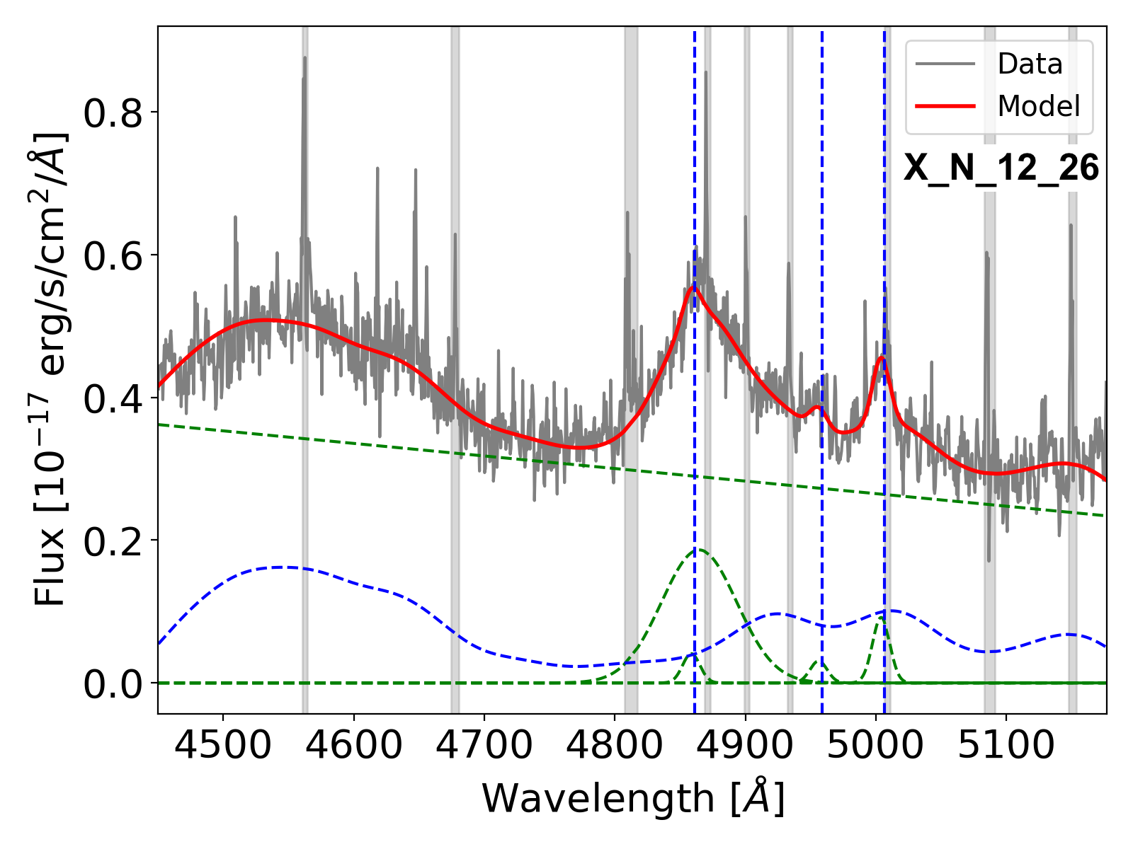
(e)

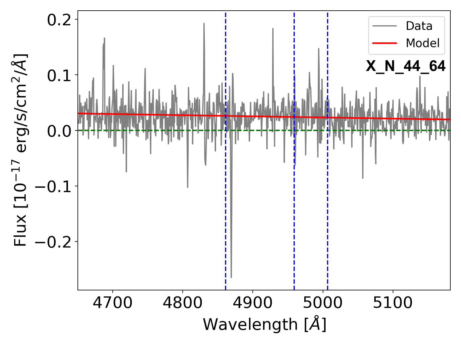
(f)

Figure 15: Integrated H-band spectrum of the SUPER targets X_N_160_22, X_N_81_44, X_N_66_23, X_N_35_20, X_N_12_26 and X_N_44_64. The grey curve shows the observed spectrum, the red curve shows the reproduced overall emission line model, the blue dashed curve shows the iron emission and the dashed green curves show the continuum emission and the individual Gaussian components (Narrow, Broad and BLR) used to reproduce the profiles of various emission lines. The blue vertical lines indicate the location of $\mathrm{H\beta}\leavevmode\nobreak\$, [O iii] $\lambda$4959 and [O iii] $\lambda$5007. The vertical grey regions mark the channels with strong skylines which were masked during the fitting procedure. The X-axis shows the rest frame wavelength after correcting for the redshift of the target and the Y-axis shows the observed flux.

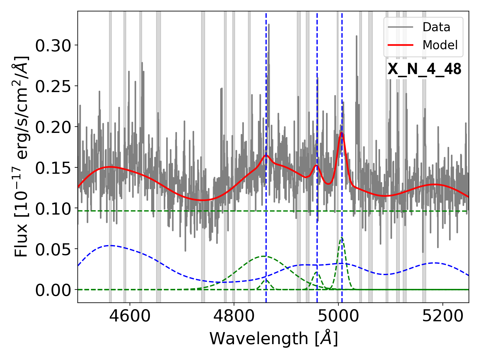
(a)

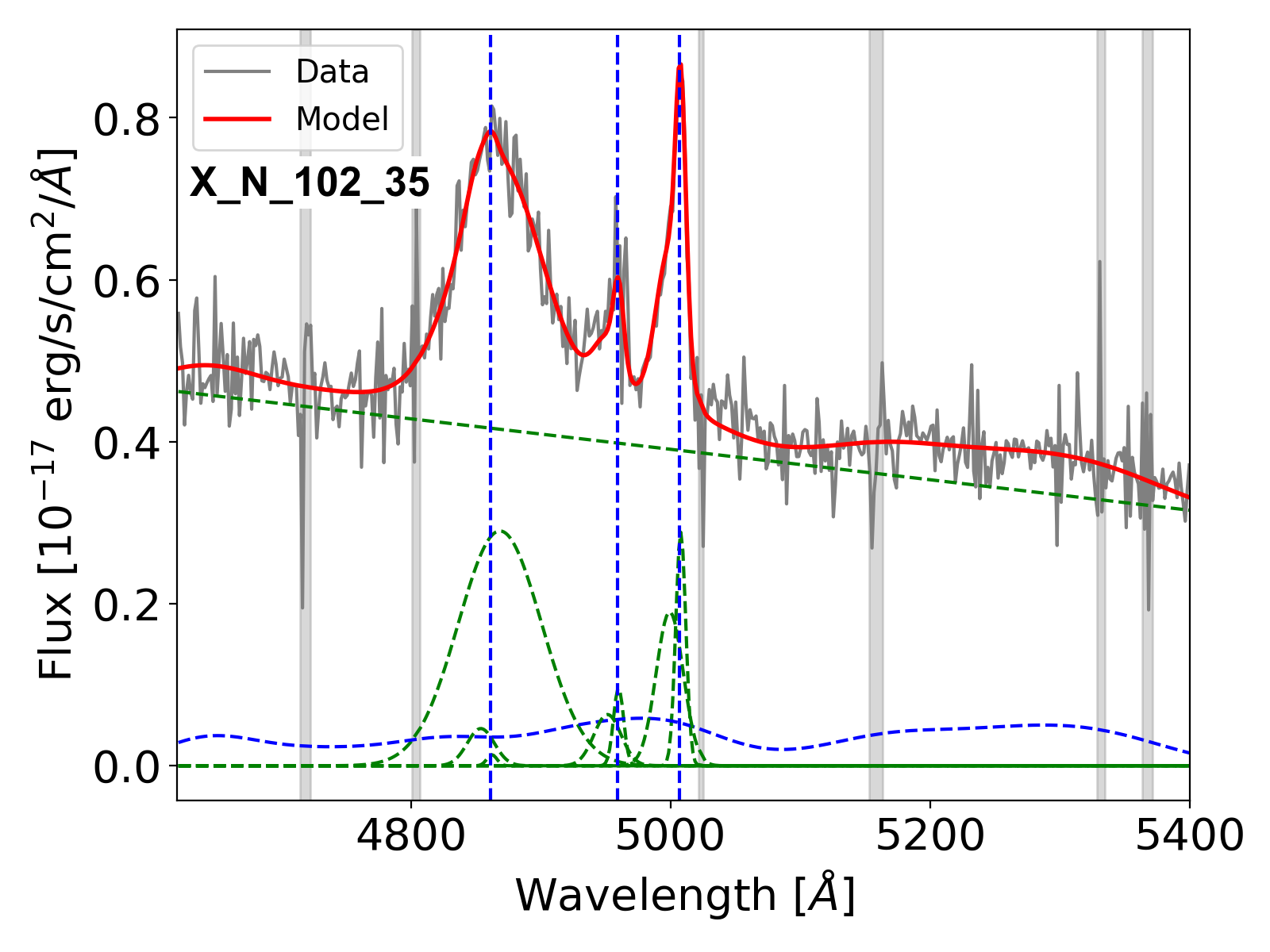
(b)

(c)

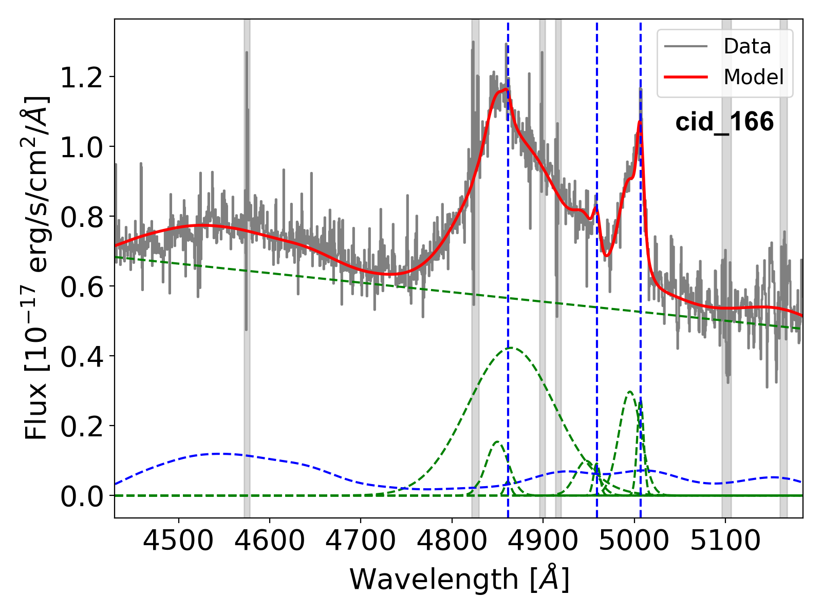
(d)

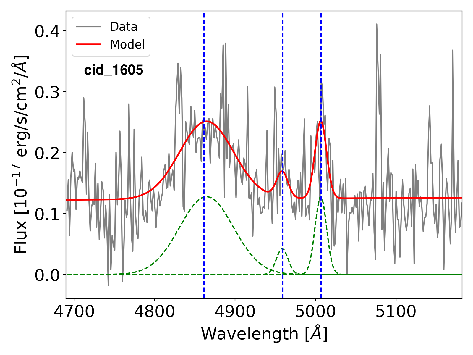
(e)

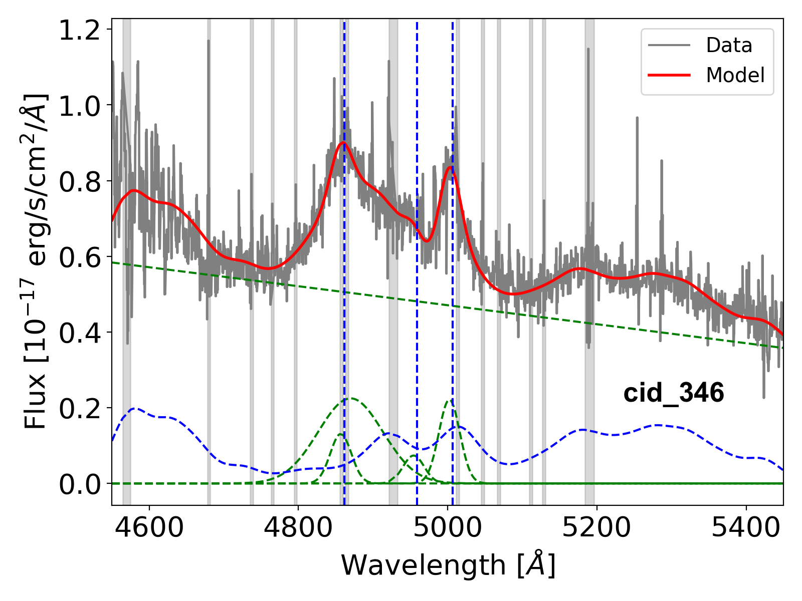
(f)

Figure 16: Same as Fig. 15 for X_N_4_48, X_N_102_35, X_N_115_23, cid_166, cid_1605 and cid_346.

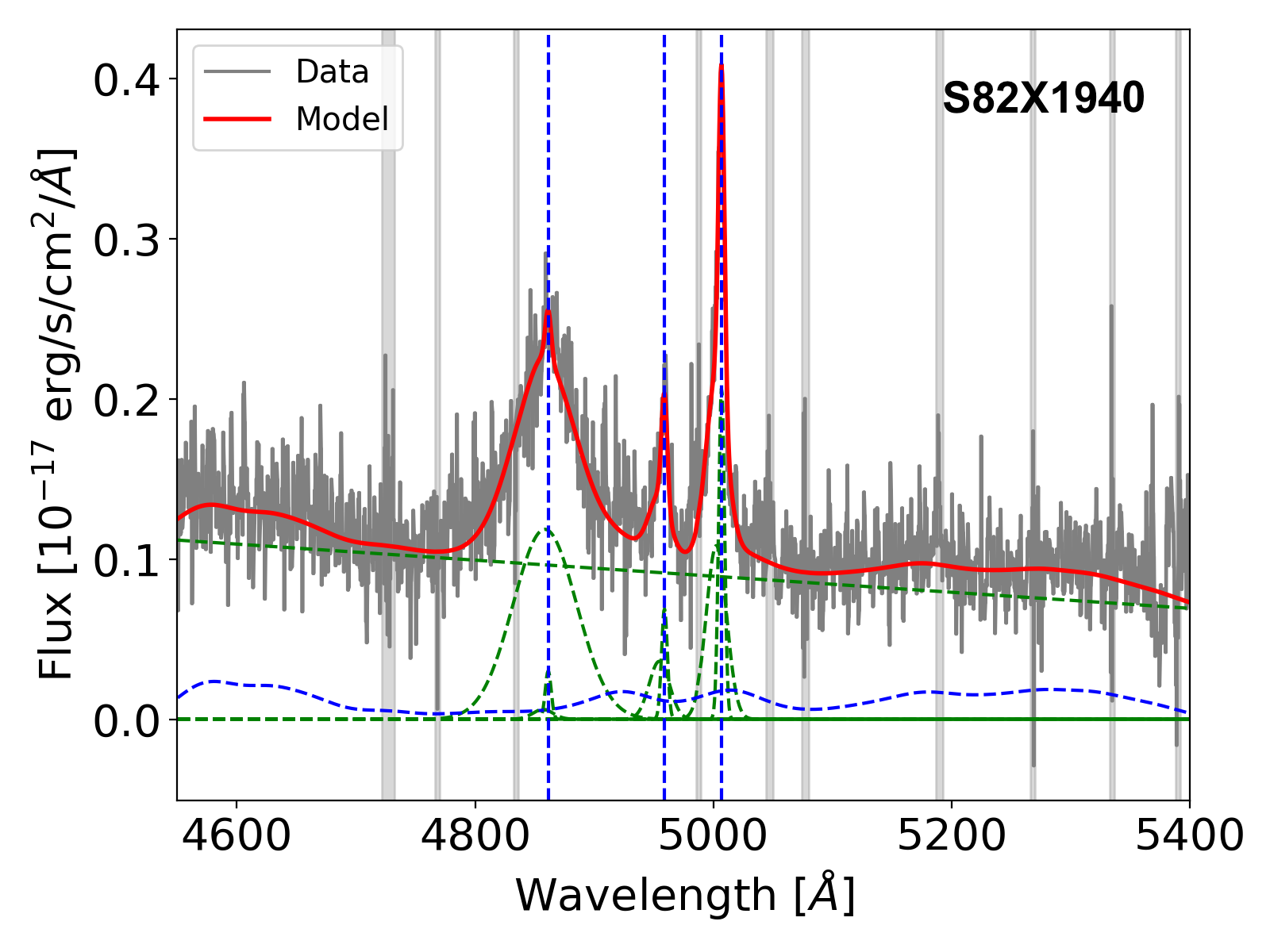
(a)

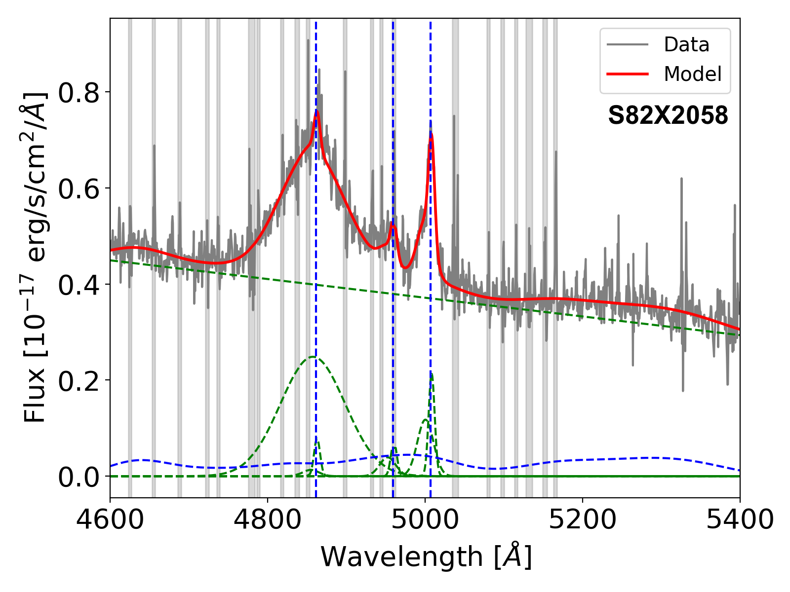
(b)

Figure 18: Same as Fig. 15 for S82X1940 and S82X2058.

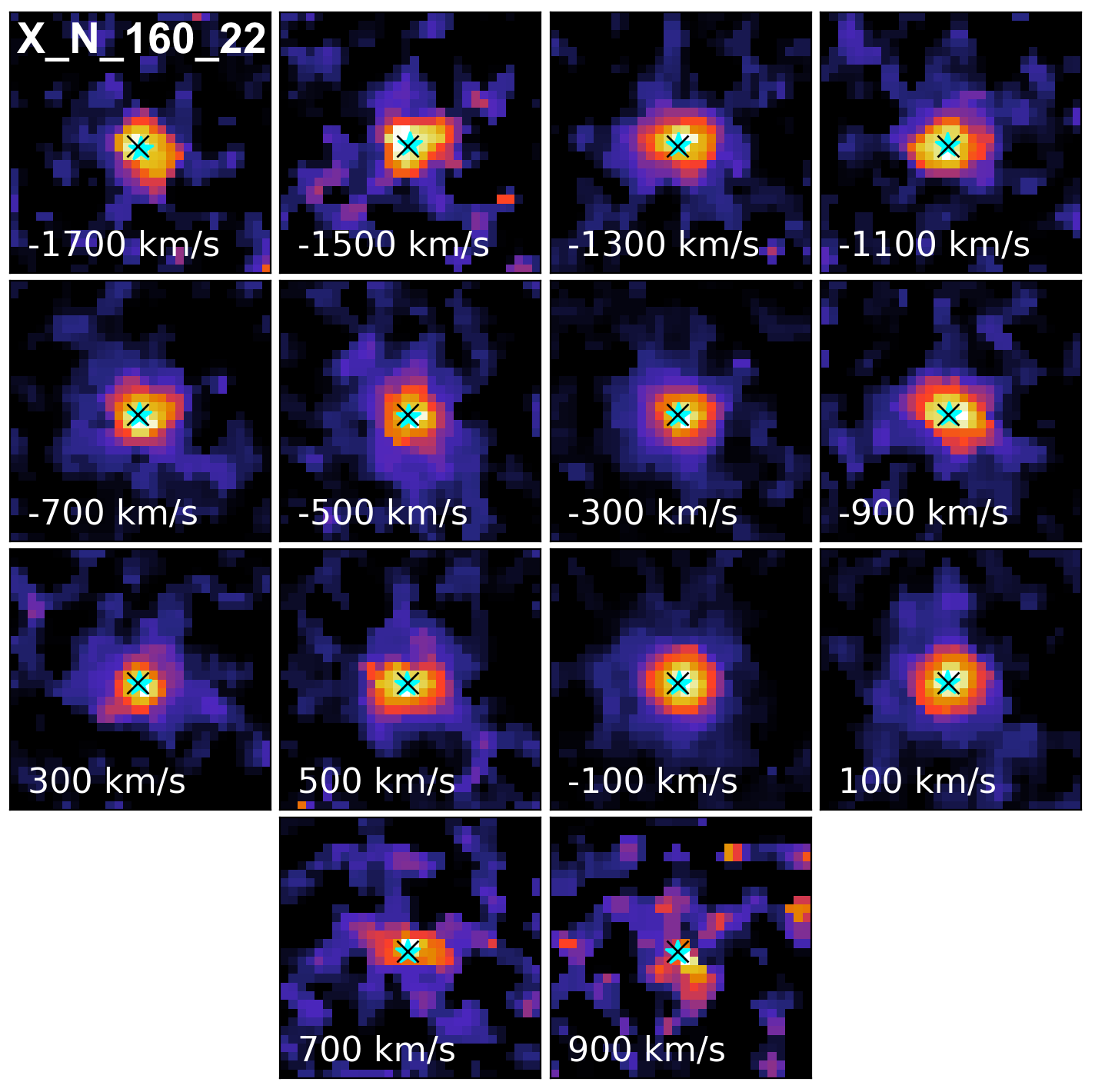
(a)

Figure 19: 1.5^′′ x 1.5^′′ [O iii] $\lambda$5007 channel maps of the SUPER target X_N_160_22 at different velocity slices, after subtracting the $\mathrm{H\beta}\leavevmode\nobreak\$, [O iii] $\lambda$4959 and iron models from the raw cube. Each velocity slice is 200 km/s wide and the displayed value is the center velocity of the respective channel. Black cross marks the location of the H-band continuum peak, used as a proxy for the AGN position. North is up and East is to left.

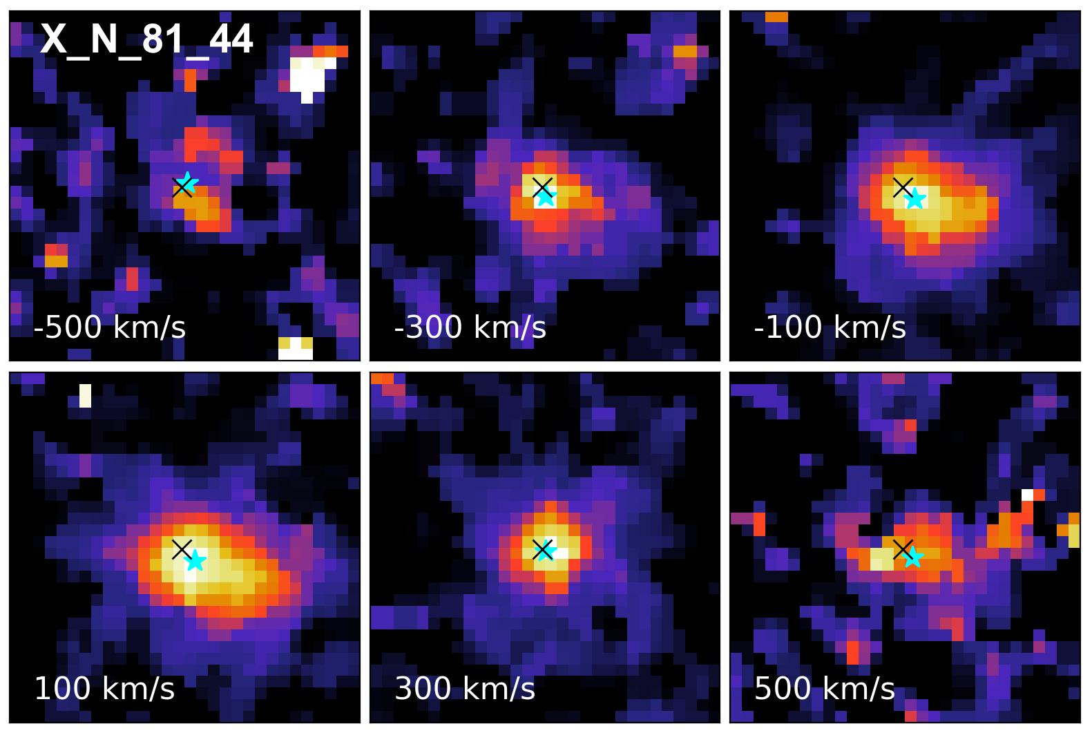
(a)

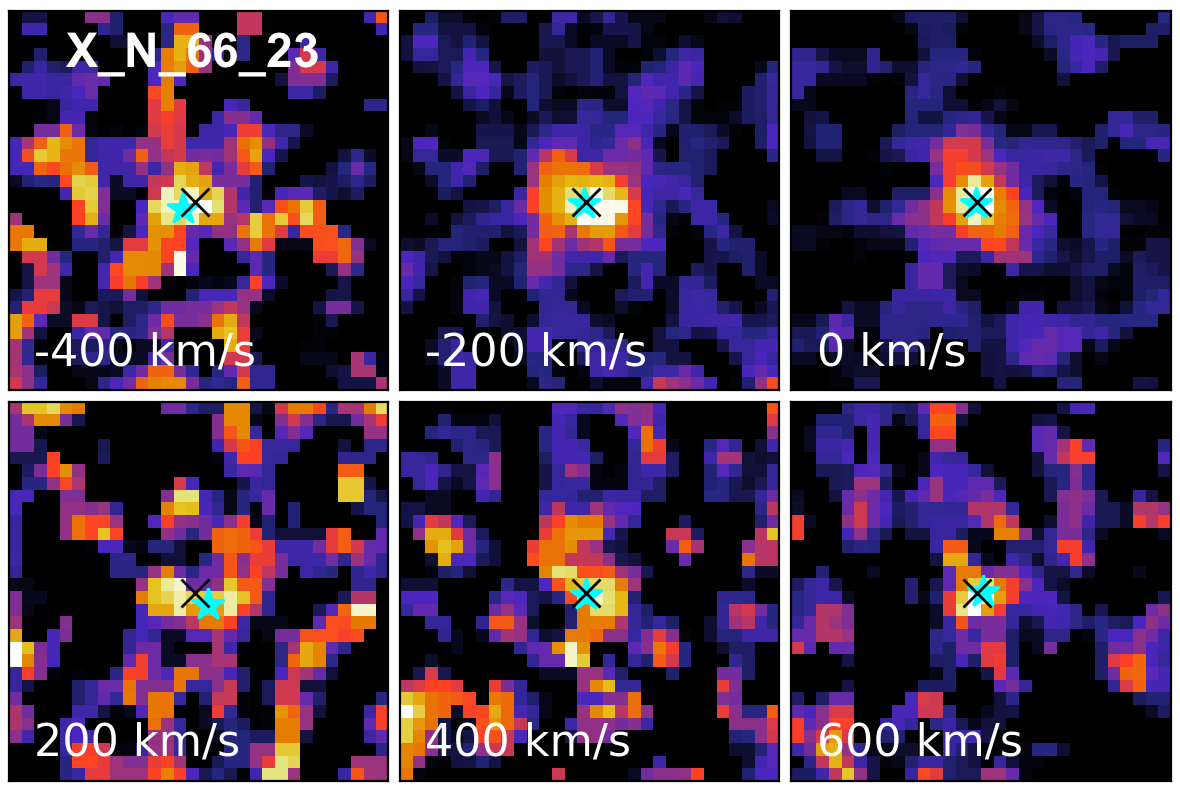
(b)

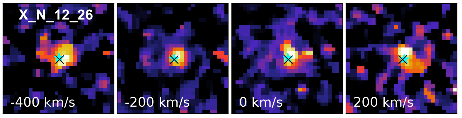
(c)

Figure 20: Same as Fig. 19 for X_N_81_44, X_N_66_23 and X_N_12_26.

(a)

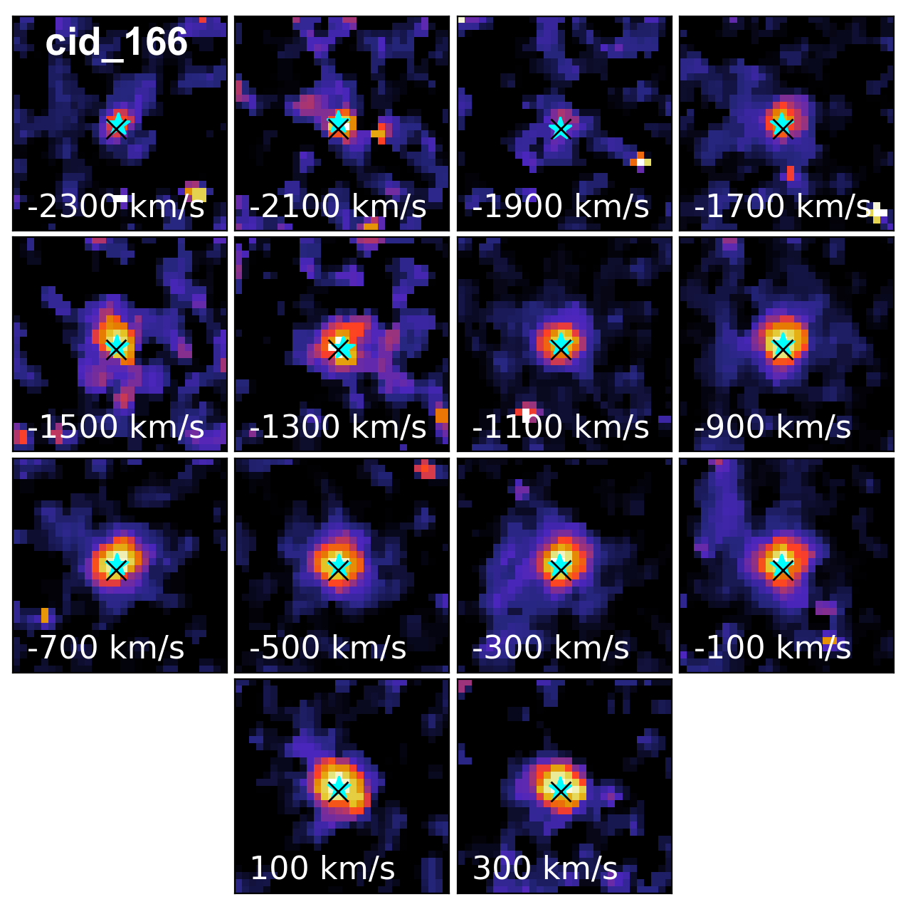
(b)

Figure 21: Same as Fig. 19 for X_N_115_23 and cid_166.

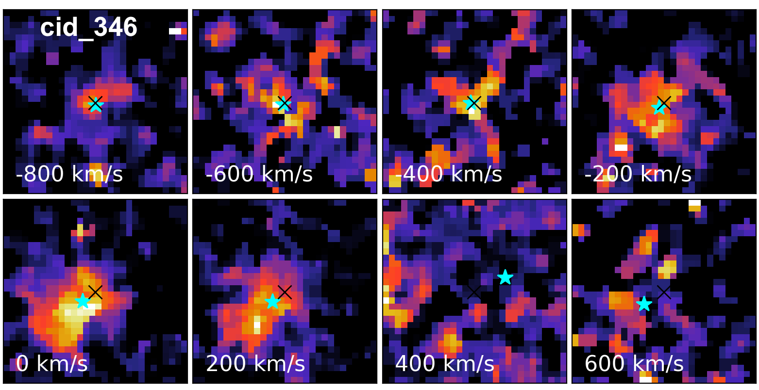
(a)

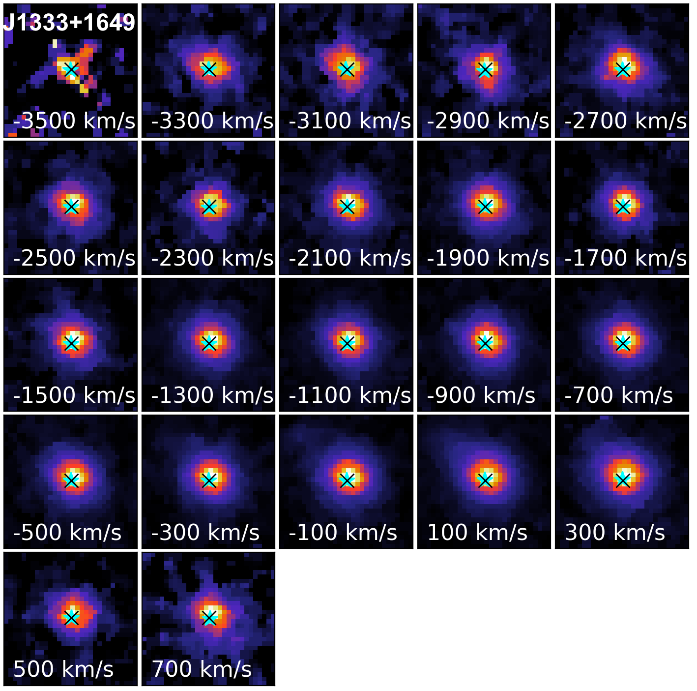
(b)

Figure 22: Same as Fig. 19 for cid_346 and J1333+1649.

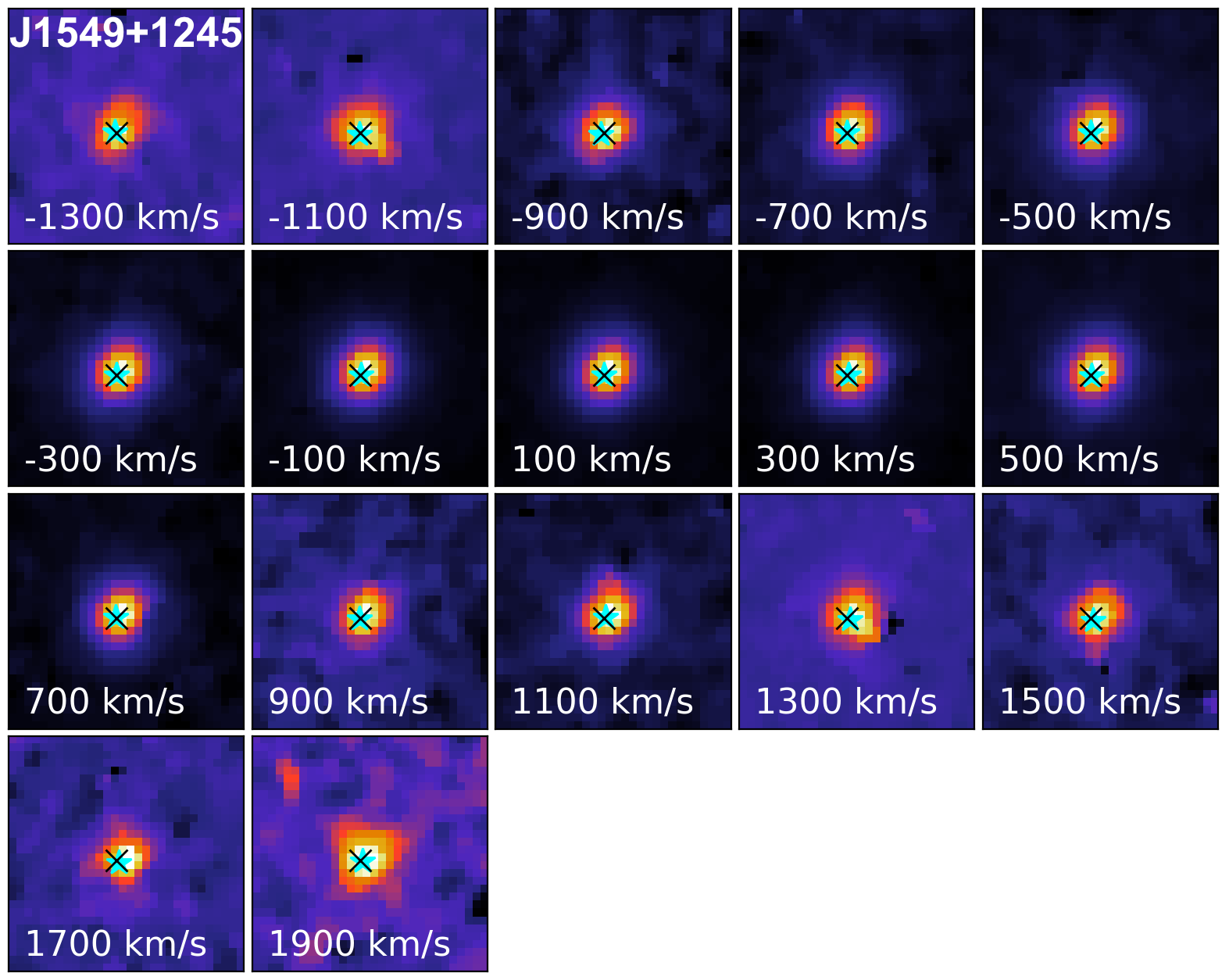
(a)

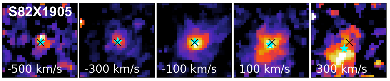
(b)

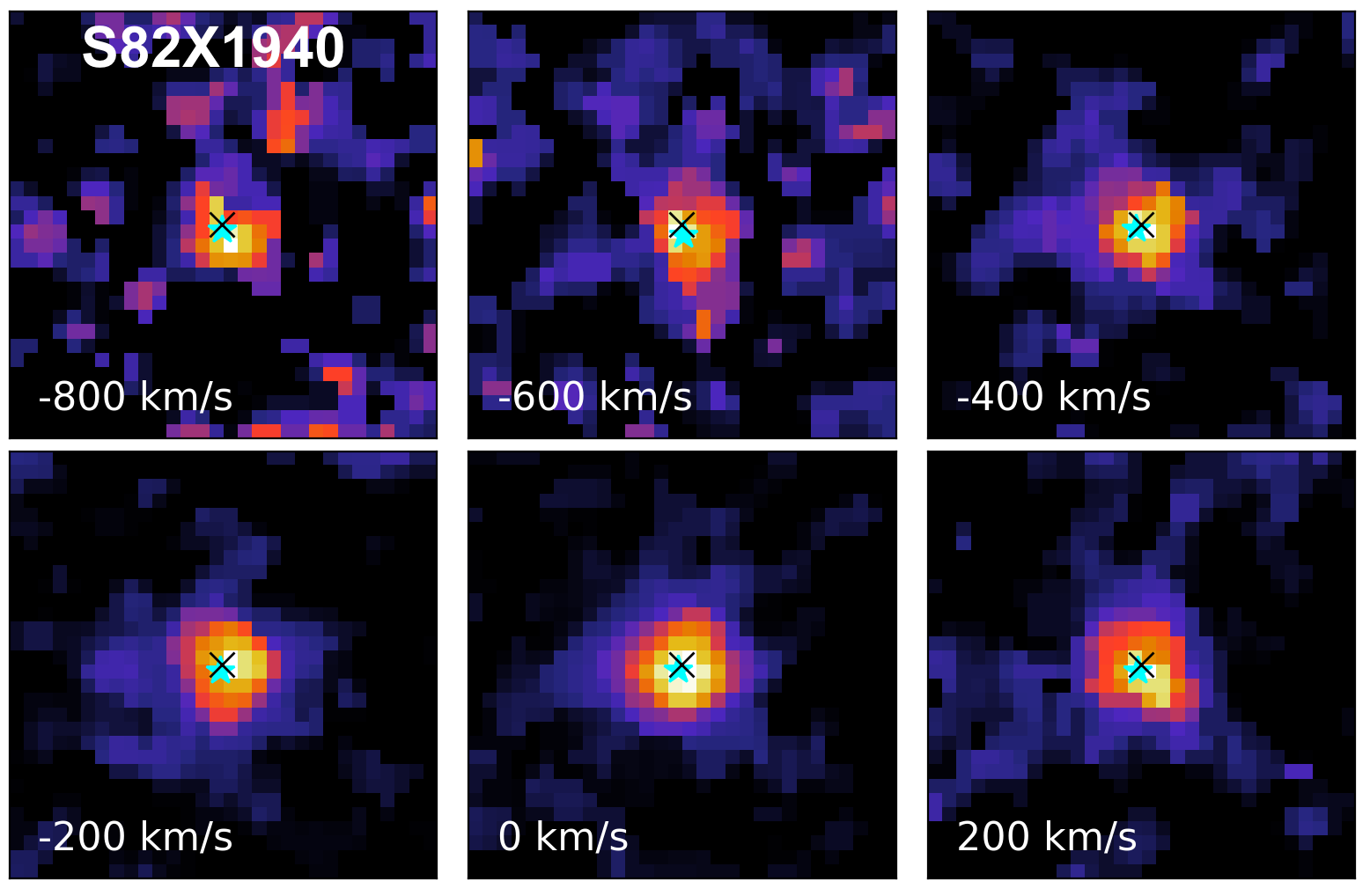
(c)

Figure 23: Same as Fig. 19 for J1549+1245, S82X1905 and S82X1940.

References

- Aalto et al. (2019) Aalto, S., Muller, S., König, S., et al. 2019, A&A, 627, A147
- Aladro et al. (2018) Aladro, R., König, S., Aalto, S., et al. 2018, A&A, 617, A20
- Alexander et al. (2010) Alexander, D. M., Swinbank, A. M., Smail, I., McDermid, R., & Nesvadba, N. P. H. 2010, MNRAS, 402, 2211
- Bae et al. (2017) Bae, H.-J., Woo, J.-H., Karouzos, M., et al. 2017, ApJ, 837, 91
- Baron & Netzer (2019) Baron, D. & Netzer, H. 2019, MNRAS, 486, 4290
- Batiste et al. (2017) Batiste, M., Bentz, M. C., Raimundo, S. I., Vestergaard, M., & Onken, C. A. 2017, ApJ, 838, L10
- Begelman (2003) Begelman, M. C. 2003, Science, 300, 1898
- Bennert et al. (2002) Bennert, N., Falcke, H., Schulz, H., Wilson, A. S., & Wills, B. J. 2002, ApJ, 574, L105
- Bischetti et al. (2017) Bischetti, M., Piconcelli, E., Vietri, G., et al. 2017, A&A, 598, A122
- Boroson & Green (1992) Boroson, T. A. & Green, R. F. 1992, ApJS, 80, 109
- Bouché et al. (2013) Bouché, N., Murphy, M. T., Kacprzak, G. G., et al. 2013, Science, 341, 50
- Brandt & Alexander (2015) Brandt, W. N. & Alexander, D. M. 2015, A&A Rev., 23, 1
- Brusa et al. (2015) Brusa, M., Bongiorno, A., Cresci, G., et al. 2015, MNRAS, 446, 2394
- Brusa et al. (2018) Brusa, M., Cresci, G., Daddi, E., et al. 2018, A&A, 612, A29
- Brusa et al. (2016) Brusa, M., Perna, M., Cresci, G., et al. 2016, A&A, 588, A58
- Bryant et al. (2015) Bryant, J. J., Owers, M. S., Robotham, A. S. G., et al. 2015, MNRAS, 447, 2857
- Bundy et al. (2015) Bundy, K., Bershady, M. A., Law, D. R., et al. 2015, ApJ, 798, 7
- Caglar et al. (2020) Caglar, T., Burtscher, L., Brandl, B., et al. 2020, A&A, 634, A114
- Cano-Díaz et al. (2012) Cano-Díaz, M., Maiolino, R., Marconi, A., et al. 2012, A&A, 537, L8
- Carniani et al. (2016) Carniani, S., Marconi, A., Maiolino, R., et al. 2016, A&A, 591, A28
- Carniani et al. (2015) Carniani, S., Marconi, A., Maiolino, R., et al. 2015, A&A, 580, A102
- Cazzoli et al. (2016) Cazzoli, S., Arribas, S., Maiolino, R., & Colina, L. 2016, A&A, 590, A125
- Choi et al. (2014) Choi, E., Naab, T., Ostriker, J. P., Johansson, P. H., & Moster, B. P. 2014, MNRAS, 442, 440
- Cicone et al. (2018) Cicone, C., Brusa, M., Ramos Almeida, C., et al. 2018, Nature Astronomy, 2, 176
- Cicone et al. (2020) Cicone, C., Maiolino, R., Aalto, S., Muller, S., & Feruglio, C. 2020, A&A, 633, A163
- Circosta et al. (2018) Circosta, C., Mainieri, V., Padovani, P., et al. 2018, A&A, 620, A82
- Civano et al. (2016) Civano, F., Marchesi, S., Comastri, A., et al. 2016, ApJ, 819, 62
- Coatman et al. (2019) Coatman, L., Hewett, P. C., Banerji, M., et al. 2019, MNRAS, 486, 5335
- Concas et al. (2019) Concas, A., Popesso, P., Brusa, M., Mainieri, V., & Thomas, D. 2019, A&A, 622, A188
- Crenshaw et al. (2010) Crenshaw, D. M., Kraemer, S. B., Schmitt, H. R., et al. 2010, AJ, 139, 871
- Cresci et al. (2009) Cresci, G., Hicks, E. K. S., Genzel, R., et al. 2009, ApJ, 697, 115
- Cresci et al. (2015) Cresci, G., Mainieri, V., Brusa, M., et al. 2015, ApJ, 799, 82
- Curran (2019) Curran, S. J. 2019, MNRAS, 484, 3911
- Curti et al. (2020) Curti, M., Maiolino, R., Cirasuolo, M., et al. 2020, MNRAS, 492, 821
- Davies et al. (2020a) Davies, R., Baron, D., Shimizu, T., et al. 2020a, arXiv e-prints, arXiv:2003.06153
- Davies (2007) Davies, R. I. 2007, MNRAS, 375, 1099
- Davies et al. (2014) Davies, R. I., Maciejewski, W., Hicks, E. K. S., et al. 2014, ApJ, 792, 101
- Davies et al. (2019) Davies, R. L., Förster Schreiber, N. M., Übler, H., et al. 2019, ApJ, 873, 122
- Davies et al. (2020b) Davies, R. L., Schreiber, N. M. F., Lutz, D., et al. 2020b, ApJ, 894, 28
- Dempsey & Zakamska (2018) Dempsey, R. & Zakamska, N. L. 2018, MNRAS, 477, 4615
- den Brok et al. (2020) den Brok, M., Carollo, C. M., Erroz-Ferrer, S., et al. 2020, MNRAS, 491, 4089
- Dimitrijević et al. (2007) Dimitrijević, M. S., Popović, L. Č., Kovačević, J., Dačić, M., & Ilić, D. 2007, MNRAS, 374, 1181
- Eisenhauer et al. (2003) Eisenhauer, F., Abuter, R., Bickert, K., et al. 2003, in Society of Photo-Optical Instrumentation Engineers (SPIE) Conference Series, Vol. 4841, Instrument Design and Performance for Optical/Infrared Ground-based Telescopes, ed. M. Iye & A. F. M. Moorwood, 1548–1561
- Emonts et al. (2017) Emonts, B. H. C., Colina, L., Piqueras-López, J., et al. 2017, A&A, 607, A116
- Faucher-Giguère & Quataert (2012) Faucher-Giguère, C.-A. & Quataert, E. 2012, MNRAS, 425, 605
- Feruglio et al. (2017) Feruglio, C., Ferrara, A., Bischetti, M., et al. 2017, A&A, 608, A30
- Fiore et al. (2017) Fiore, F., Feruglio, C., Shankar, F., et al. 2017, A&A, 601, A143
- Fluetsch et al. (2019) Fluetsch, A., Maiolino, R., Carniani, S., et al. 2019, MNRAS, 483, 4586
- Förster Schreiber et al. (2018) Förster Schreiber, N. M., Renzini, A., Mancini, C., et al. 2018, ApJS, 238, 21
- Förster Schreiber et al. (2019) Förster Schreiber, N. M., Übler, H., Davies, R. L., et al. 2019, ApJ, 875, 21
- Fruchter & Hook (2002) Fruchter, A. S. & Hook, R. N. 2002, PASP, 114, 144
- Gallagher et al. (2019) Gallagher, R., Maiolino, R., Belfiore, F., et al. 2019, MNRAS, 485, 3409
- García-Burillo et al. (2014) García-Burillo, S., Combes, F., Usero, A., et al. 2014, A&A, 567, A125
- Gebhardt et al. (2000) Gebhardt, K., Bender, R., Bower, G., et al. 2000, ApJ, 539, L13
- Georgakakis & Nandra (2011) Georgakakis, A. & Nandra, K. 2011, MNRAS, 414, 992
- Hainline et al. (2014) Hainline, K. N., Hickox, R. C., Greene, J. E., et al. 2014, ApJ, 787, 65
- Harrison et al. (2016) Harrison, C. M., Alexander, D. M., Mullaney, J. R., et al. 2016, MNRAS, 456, 1195
- Harrison et al. (2014) Harrison, C. M., Alexander, D. M., Mullaney, J. R., & Swinbank, A. M. 2014, MNRAS, 441, 3306
- Harrison et al. (2012) Harrison, C. M., Alexander, D. M., Swinbank, A. M., et al. 2012, MNRAS, 426, 1073
- Harrison et al. (2018) Harrison, C. M., Costa, T., Tadhunter, C. N., et al. 2018, Nature Astronomy, 2, 198
- Hill & Zakamska (2014) Hill, M. J. & Zakamska, N. L. 2014, MNRAS, 439, 2701
- Hopkins et al. (2016) Hopkins, P. F., Torrey, P., Faucher-Giguère, C.-A., Quataert, E., & Murray, N. 2016, MNRAS, 458, 816
- Husemann et al. (2017) Husemann, B., Davis, T. A., Jahnke, K., et al. 2017, MNRAS, 470, 1570
- Husemann et al. (2014) Husemann, B., Jahnke, K., Sánchez, S. F., et al. 2014, MNRAS, 443, 755
- Husemann et al. (2016) Husemann, B., Scharwächter, J., Bennert, V. N., et al. 2016, A&A, 594, A44
- Husemann et al. (2019) Husemann, B., Scharwächter, J., Davis, T. A., et al. 2019, A&A, 627, A53
- Husemann et al. (2013) Husemann, B., Wisotzki, L., Sánchez, S. F., & Jahnke, K. 2013, A&A, 549, A43
- Ishibashi & Fabian (2016) Ishibashi, W. & Fabian, A. C. 2016, MNRAS, 457, 2864
- Ishibashi et al. (2019) Ishibashi, W., Fabian, A. C., & Reynolds, C. S. 2019, MNRAS, 486, 2210
- Jahnke et al. (2004) Jahnke, K., Wisotzki, L., Sánchez, S. F., et al. 2004, Astronomische Nachrichten, 325, 128
- Kakkad et al. (2018) Kakkad, D., Groves, B., Dopita, M., et al. 2018, A&A, 618, A6
- Kakkad et al. (2016) Kakkad, D., Mainieri, V., Padovani, P., et al. 2016, A&A, 592, A148
- Karouzos et al. (2016) Karouzos, M., Woo, J.-H., & Bae, H.-J. 2016, ApJ, 819, 148
- King (2003) King, A. 2003, ApJ, 596, L27
- King & Pounds (2015) King, A. & Pounds, K. 2015, ARA&A, 53, 115
- Krug et al. (2010) Krug, H. B., Rupke, D. S. N., & Veilleux, S. 2010, ApJ, 708, 1145
- LaMassa et al. (2016) LaMassa, S. M., Urry, C. M., Cappelluti, N., et al. 2016, ApJ, 817, 172
- Läsker et al. (2016) Läsker, R., Greene, J. E., Seth, A., et al. 2016, ApJ, 825, 3
- Leighly (1999) Leighly, K. M. 1999, ApJS, 125, 317
- Leung et al. (2019) Leung, G. C. K., Coil, A. L., Aird, J., et al. 2019, ApJ, 886, 11
- Liu et al. (2013) Liu, G., Zakamska, N. L., Greene, J. E., Nesvadba, N. P. H., & Liu, X. 2013, MNRAS, 436, 2576
- Liu et al. (2016) Liu, Z., Merloni, A., Georgakakis, A., et al. 2016, MNRAS, 459, 1602
- Luo et al. (2017) Luo, B., Brandt, W. N., Xue, Y. Q., et al. 2017, ApJS, 228, 2
- Madau & Dickinson (2014) Madau, P. & Dickinson, M. 2014, ARA&A, 52, 415
- Magorrian et al. (1998) Magorrian, J., Tremaine, S., Richstone, D., et al. 1998, AJ, 115, 2285
- Maiolino et al. (2017) Maiolino, R., Russell, H. R., Fabian, A. C., et al. 2017, Nature, 544, 202
- Martocchia et al. (2017) Martocchia, S., Piconcelli, E., Zappacosta, L., et al. 2017, A&A, 608, A51
- May et al. (2018) May, D., Rodríguez-Ardila, A., Prieto, M. A., et al. 2018, MNRAS, 481, L105
- McElroy et al. (2015) McElroy, R., Croom, S. M., Pracy, M., et al. 2015, MNRAS, 446, 2186
- Menci et al. (2019) Menci, N., Fiore, F., Feruglio, C., et al. 2019, ApJ, 877, 74
- Menci et al. (2008) Menci, N., Fiore, F., Puccetti, S., & Cavaliere, A. 2008, ApJ, 686, 219
- Menzel et al. (2016) Menzel, M. L., Merloni, A., Georgakakis, A., et al. 2016, MNRAS, 457, 110
- Michiyama et al. (2018) Michiyama, T., Iono, D., Sliwa, K., et al. 2018, ApJ, 868, 95
- Müller-Sánchez et al. (2011) Müller-Sánchez, F., Prieto, M. A., Hicks, E. K. S., et al. 2011, ApJ, 739, 69
- Muratov et al. (2015) Muratov, A. L., Kereš, D., Faucher-Giguère, C.-A., et al. 2015, MNRAS, 454, 2691
- Nesvadba et al. (2017) Nesvadba, N. P. H., De Breuck, C., Lehnert, M. D., Best, P. N., & Collet, C. 2017, A&A, 599, A123
- Nesvadba et al. (2006) Nesvadba, N. P. H., Lehnert, M. D., Eisenhauer, F., et al. 2006, ApJ, 650, 693
- Nims et al. (2015) Nims, J., Quataert, E., & Faucher-Giguère, C.-A. 2015, MNRAS, 447, 3612
- Padovani et al. (2017) Padovani, P., Alexander, D. M., Assef, R. J., et al. 2017, A&A Rev., 25, 2
- Perna et al. (2015) Perna, M., Brusa, M., Cresci, G., et al. 2015, A&A, 574, A82
- Perna et al. (2019) Perna, M., Cresci, G., Brusa, M., et al. 2019, A&A, 623, A171
- Perna et al. (2017) Perna, M., Lanzuisi, G., Brusa, M., Cresci, G., & Mignoli, M. 2017, A&A, 606, A96
- Perrotta et al. (2019) Perrotta, S., Hamann, F., Zakamska, N. L., et al. 2019, MNRAS, 488, 4126
- Petric et al. (2018) Petric, A. O., Armus, L., Flagey, N., et al. 2018, AJ, 156, 295
- Radovich et al. (2019) Radovich, M., Poggianti, B., Jaffé, Y. L., et al. 2019, MNRAS, 486, 486
- Rakshit & Woo (2018) Rakshit, S. & Woo, J.-H. 2018, ApJ, 865, 5
- Revalski et al. (2018) Revalski, M., Dashtamirova, D., Crenshaw, D. M., et al. 2018, ApJ, 867, 88
- Riffel et al. (2015) Riffel, R. A., Storchi-Bergmann, T., & Riffel, R. 2015, MNRAS, 451, 3587
- Riffel et al. (2013) Riffel, R. A., Storchi-Bergmann, T., & Winge, C. 2013, MNRAS, 430, 2249
- Riffel et al. (2020) Riffel, R. A., Zakamska, N. L., & Riffel, R. 2020, MNRAS, 491, 1518
- Roberts-Borsani (2020) Roberts-Borsani, G. W. 2020, MNRAS
- Rodríguez-Ardila et al. (2000) Rodríguez-Ardila, A., Binette, L., Pastoriza, M. G., & Donzelli, C. J. 2000, ApJ, 538, 581
- Rupke et al. (2002) Rupke, D. S., Veilleux, S., & Sanders, D. B. 2002, ApJ, 570, 588
- Rupke et al. (2017) Rupke, D. S. N., Gültekin, K., & Veilleux, S. 2017, ApJ, 850, 40
- Rupke & Veilleux (2011) Rupke, D. S. N. & Veilleux, S. 2011, ApJ, 729, L27
- Rupke & Veilleux (2013) Rupke, D. S. N. & Veilleux, S. 2013, ApJ, 768, 75
- Sánchez et al. (2012) Sánchez, S. F., Kennicutt, R. C., Gil de Paz, A., et al. 2012, A&A, 538, A8
- Scholtz et al. (2020) Scholtz, J., Harrison, C. M., Rosario, D. J., et al. 2020, MNRAS, 492, 3194
- Schutte et al. (2019) Schutte, Z., Reines, A. E., & Greene, J. E. 2019, ApJ, 887, 245
- Serafinelli et al. (2019) Serafinelli, R., Tombesi, F., Vagnetti, F., et al. 2019, A&A, 627, A121
- Shankar et al. (2009) Shankar, F., Weinberg, D. H., & Miralda-Escudé, J. 2009, ApJ, 690, 20
- Shimizu et al. (2019) Shimizu, T. T., Davies, R. I., Lutz, D., et al. 2019, MNRAS, 490, 5860
- Skrutskie et al. (2006) Skrutskie, M. F., Cutri, R. M., Stiening, R., et al. 2006, AJ, 131, 1163
- Steidel et al. (2010) Steidel, C. C., Erb, D. K., Shapley, A. E., et al. 2010, ApJ, 717, 289
- Storey & Zeippen (2000) Storey, P. J. & Zeippen, C. J. 2000, MNRAS, 312, 813
- Stott et al. (2016) Stott, J. P., Swinbank, A. M., Johnson, H. L., et al. 2016, MNRAS, 457, 1888
- Swinbank et al. (2019) Swinbank, A. M., Harrison, C. M., Tiley, A. L., et al. 2019, MNRAS, 487, 381
- Tacconi et al. (2020) Tacconi, L. J., Genzel, R., & Sternberg, A. 2020, arXiv e-prints, arXiv:2003.06245
- Tadhunter et al. (2014) Tadhunter, C., Morganti, R., Rose, M., Oonk, J. B. R., & Oosterloo, T. 2014, Nature, 511, 440
- Thomas et al. (2017) Thomas, A. D., Dopita, M. A., Shastri, P., et al. 2017, ApJS, 232, 11
- Tsuzuki et al. (2006) Tsuzuki, Y., Kawara, K., Yoshii, Y., et al. 2006, ApJ, 650, 57
- Vayner et al. (2017) Vayner, A., Wright, S. A., Murray, N., et al. 2017, ApJ, 851, 126
- Veilleux et al. (2020) Veilleux, S., Maiolino, R., Bolatto, A. D., & Aalto, S. 2020, A&A Rev., 28, 2
- Veilleux et al. (2009) Veilleux, S., Rupke, D. S. N., & Swaters, R. 2009, ApJ, 700, L149
- Venturi et al. (2018) Venturi, G., Nardini, E., Marconi, A., et al. 2018, A&A, 619, A74
- Véron-Cetty et al. (2004) Véron-Cetty, M. P., Joly, M., & Véron, P. 2004, A&A, 417, 515
- Vietri (2020) Vietri, G. 2020, et. al. in prep
- Vietri et al. (2018) Vietri, G., Piconcelli, E., Bischetti, M., et al. 2018, A&A, 617, A81
- Villar-Martín et al. (2016) Villar-Martín, M., Arribas, S., Emonts, B., et al. 2016, MNRAS, 460, 130
- Wagner et al. (2013) Wagner, A. Y., Umemura, M., & Bicknell, G. V. 2013, ApJ, 763, L18
- Whitaker et al. (2014) Whitaker, K. E., Rigby, J. R., Brammer, G. B., et al. 2014, ApJ, 790, 143
- Wilkins et al. (2019) Wilkins, S. M., Lovell, C. C., & Stanway, E. R. 2019, MNRAS, 490, 5359
- Wisnioski et al. (2019) Wisnioski, E., Förster Schreiber, N. M., Fossati, M., et al. 2019, ApJ, 886, 124
- Wylezalek et al. (2020) Wylezalek, D., Flores, A. M., Zakamska, N. L., Greene, J. E., & Riffel, R. A. 2020, MNRAS, 492, 4680
- Wylezalek et al. (2016) Wylezalek, D., Zakamska, N. L., Liu, G., & Obied, G. 2016, MNRAS, 457, 745
- Zakamska & Greene (2014) Zakamska, N. L. & Greene, J. E. 2014, MNRAS, 442, 784
- Zakamska et al. (2016) Zakamska, N. L., Hamann, F., Pâris, I., et al. 2016, MNRAS, 459, 3144
- Zappacosta et al. (2020) Zappacosta, L., Piconcelli, E., Giustini, M., et al. 2020, A&A, 635, L5
- Zschaechner et al. (2018) Zschaechner, L. K., Bolatto, A. D., Walter, F., et al. 2018, ApJ, 867, 111
- Zubovas (2018) Zubovas, K. 2018, MNRAS, 479, 3189
- Zubovas & King (2012) Zubovas, K. & King, A. 2012, ApJ, 745, L34
- Zubovas & Nayakshin (2014) Zubovas, K. & Nayakshin, S. 2014, MNRAS, 440, 2625