An improved Bayesian TRIE based model for SMS text normalization

Abstract

Normalization of SMS text, commonly known as texting language, is being pursued for more than a decade. A probabilistic approach based on the Trie data structure was proposed in literature which was found to be better performing than HMM based approaches proposed earlier in predicting the correct alternative for an out-of-lexicon word. However, success of the Trie-based approach depends largely on how correctly the underlying probabilities of word occurrences are estimated. In this work we propose a structural modification to the existing Trie-based model along with a novel training algorithm and probability generation scheme. We prove two theorems on statistical properties of the proposed Trie and use them to claim that is an unbiased and consistent estimator of the occurrence probabilities of the words. We further fuse our model into the paradigm of noisy channel based error correction and provide a heuristic to go beyond a Damerau–Levenshtein distance of one.
Keywords: SMS text normalization, Noisy channel, Trie, Theory of estimation

1 Introduction

SMS text normalization focuses on translating texting language, often filled with abbreviations and marred by typing errors into plain English text. With the smartphone revolution and massive popularisation of social media platforms, users often transmit messages consisting of up to thousands of words in a single day. However, these text messages consist of numerous abbreviations and errors. This often arises due to a lack of formalities between users, human error, and in more severe cases due to disabilities. With an increase in the screen sizes, this is becoming more of a concern especially when the user resorts to one handed typing. Thus, shorter message length and semantic unambiguity end up working antagonistically which gives shape to a compressed, non-standard form of language called NetSpeak [1], commonly known as the texting language. Unfortunately, traditional NLP methods perform rather poorly when dealing with these kinds of texts [2]. As described in [3], texting language contains many non-standard abbreviations, have unique characteristics and behave quite differently which may be the reason for poor performance of traditional NLP methods.

In [4] the problem was approached by leveraging the phonetic information but required a dictionary for phonetic transcription. [5] used a dictionary for erroneous words but used an ambiguous ranking mechanism. [6] used a completely heuristic rule based model and employed a dictionary for typos as well which in all the three cases caused the time complexity to grow with the size of the dictionary. [7] compared machine translation models such as SMT and NMT and showed their critical dependence on high quality training data. In [8], a Hidden Markov Model based approach was used for each word present in the corpus to model all possible normalized or corrected texts and their probabilities of occurrence. This was further used to rank all the possible normalised words and the highest ranking word would be selected for output as the semantically correct word. In [9], a Trie based probability generation model was proposed, and was shown to outperform HMM-based models whenever the incorrect word was within an edit distance one after prepossessing for phonetic errors. However, in some cases the target word did not end up having the highest rank. For example, ‘mate’, the intended target word was ranked $4^{th}$ in the suggestions list for the word ‘m8’.
Through this work we address the limitations of this Trie based probability generation model. We make a set of improvements over the scheme proposed in [9] which we consider to be the baseline system for the present work. Firstly, unlike [9] where a new word is added in a Trie only once when it is encountered for the first time during the training phase, a dynamic training environment is used in the proposed model. In the proposed model the Trie is initially constructed with a certain corpus of most commonly used words and is then deployed. After deployment, the tries learns dynamically from the texting habits of the users over time i.e. it keeps adding the same words repeatedly as and when they are encountered. We show that the new model in the described environment is able to estimate the real probability of occurrence of a word through its own new probability generating algorithm. Hence it facilitates 0-1 loss minimisation in a decision theoretic setup. This in turn minimizes the chances of the target word not being ranked as the highest one.
Additionally, as explained in [10] , it is computationally infeasible to generate all the words which are at an edit distance two from a given word. This limited the spelling correction abilities of the baseline model. In this work we propose some novel heuristics that help in overcoming the above shortcoming significantly.
The contributions of the present work are

1. We suggest a structural modification to the Trie-based reasoning scheme to improve model accuracy and performance.

2. We prove mathematically that in the described dynamic environment, the expectation of the thus generated Trie probability equals the occurrence probability for each word.

3. We further prove that the Trie probability of each word in the corpus almost surely(a.s.) converges to its occurrence probability.

4. Develop a set of heuristics for error correction.

5. Provide empirical results through simulations to support the presented theorems and highlight the superiority of the new model.

2 Background

From existing literature on the behaviour of users while using texting language [11], one can classify most of the linguistic errors as:

1. Insertion Error: Insertion of an extra alphabet in the word. Eg. ‘hoarding’$\rightarrow$‘hoardingh’

2. Deletion Error: Deletion of an alphabet from the word. Eg. ‘mobile’$\rightarrow$‘moble’

3. Replacement Error: Replacement of an alphabet by another in the word. Eg. ‘amazing’$\rightarrow$‘anazing’

4. Swap Error: Swapping of two adjacent characters in the word. Eg. ‘care’$\rightarrow$‘caer’

5. Phonetic Error: A group of alphabets is replaced by another group of alphabets or numbers having the same sound. Eg. ‘tomorrow’$\rightarrow$‘2morrow’

To deal with these errors, an elaborate error correction algorithm has already been proposed in the baseline model wherein given an erroneous/non-lexical word, a suggestion list of possible target words was prepared. The probability of occurrence for each word in the list was generated using a Trie based algorithm as described in Section 2.2 which was used for ranking the words in the suggestion list. The highest ranking word was given out as the likely intended word.

2.1 Design of the TRIE

Trie is a memory efficient data structure primarily used for storing of words. The search complexity in the data structure is $\mathcal{O}$($M$), where $M$ represents the number of characters in the longest word stored in the Trie which makes it a computationally efficient data structure for the problem.
Each node contains an integer variable Count and a Boolean variable End-Of-Word. The Trie is set up by initializing it with a number of English words. Count for each node is initiated to zero and incremented by one each time a word is inserted through that node. End-Of-Word represents if a word ends at the given node and is set to True at the ending node of each word. Each time a new word is inserted, the Count variables of the passing nodes are updated and if at any point the next node is not already present for the insertion of a character, a new node is created and added as a child. At the end of the new word, End-Of-Word is switched from False to True.

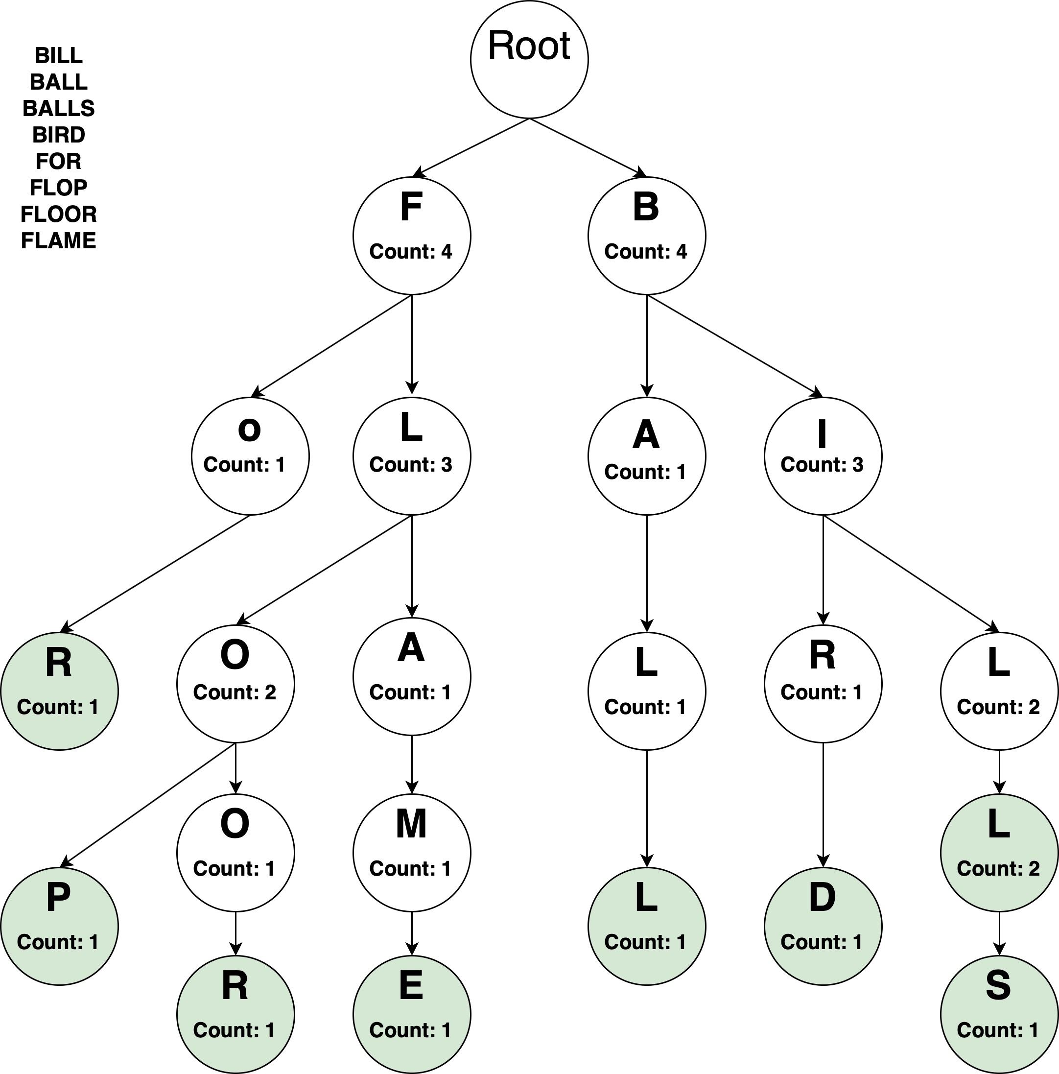
Fig. 1: Trie: The model has been trained with 8 words each once. Green represents a True value for End-Of-Word for the coloured node.

2.2 TRIE probability of a Word

Assigning probability of occurrence to a word through the Trie is a task of prime importance in the model. In the baseline model this was done in a simplistic manner as described below.
The probability of choosing the $i^{th}$ child node was estimated by dividing its Count variable, to be referred as Count(i) by Total(i) which was defined as:

$$Total(i)=Count(i)+\sum_{j\in Sibling(i)}Count(j)$$ (1)

Where Sibling(i) refers to the set of all the other child nodes of the common parent node. Hence the probability of the $i^{th}$ child node was set to be:

$$P(i)=\frac{Count(i)}{Total(i)}$$ (2)

Further, to get the probability of a string $s_{1}s_{2}\ldots s_{n}$ from the Trie, the conditional rule of probability was used as:

$$P(s_{1}s_{2}\ldots s_{n})=P(s_{1})P(s_{2}|s_{1})\ldots P(s_{n}|s_{1}s_{2}\ldots s_{n-1})$$

For example, consider the string ’bird’, then

$$P(bird)=P(b)P(i|b)P(r|bi)P(d|bir)$$

Hence, from Fig.1 we get that $P(bird)=\frac{1}{2}\times\frac{3}{4}\times\frac{1}{3}\times\frac{1}{1}=\frac{1}{8}$.

3 The Improved Trie

We consider the user to be modelled as a corpus of words denoted by $\mathcal{S}$ where each word $w_{i}\in\mathcal{S}$ has an occurrence probability of $p_{i}$. Note that then the training and probability calculations as proposed in the baseline Trie does not account for an important case. This is when the corpus of words $\mathcal{S}$ contains two words say $w_{1}$ and $w_{2}$ with occurrence probabilities $p_{1}$ and $p_{2}$, $p_{1}\neq p_{2}$ such that $w_{1}$ is a prefix of $w_{2}$ or vice versa. For example consider the two words ’bill’ and ’bills’ in Fig.1. No matter what the occurrence probabilities of those two words are, they will always end up with the same Trie probability even after training the Trie a large number of times after random sampling from $\mathcal{S}$. While the deviation from occurrence probabilities might not vary a lot in the example considered since one word happens to be the plural of the other, it will matter much more in words such as ’lips’ & ’lipstick’ and ‘dear’ & ‘dearth’.
To overcome this we propose the introduction of a dummy node. This dummy node is added as a child of every node which has End-Of-Word set as True but has at least one non-dummy node as its child. The Count variable of this dummy node is set to be the count variable of the parent reduced by the count variable of all the siblings of the new dummy node.

$$Count(D)=Count(P)-\sum_{j\in Siblings(D)}Count(j)$$ (3)

Where $D$ denotes the dummy node and $P$ denotes the parent of the dummy node. Algorithm I in this section outlines the procedure for training the new Trie as described above.
In addition to the training algorithm, we also propose Algorithm II which is used to generate the Trie probability of a given string.
Further, to justify usage of the new Trie mathematically, the proposed training algorithm and the algorithm for the Trie probability generation, we present Theorem 3.1, Theorem 3.2 and Corollary 3.3.

  Algorithm I: The Training   Input: $w$, root
Initialization: $str\leftarrow w$, $m\leftarrow str$.length, $parent\leftarrow$ root, $Flag\leftarrow 0$
For $j\leftarrow 1$ to $m$

1. If $parent$.children does not contain $str$.charAt[$j$] node

   1. Insert new node corresponding to $str$.charAt[$j$]

   2. $Flag\leftarrow 1$

2. $parent\leftarrow$ child corresponding to $str$.charAt[$j$]

3. $parent$.Counter $\leftarrow parent$.Counter$+1$

$parent$.End-Of-Word$\leftarrow$True
If a dummy node $D$ is already a child of $parent$

1. Increment Counter of $D$ by 1

Else if $Flag$ is 0 and $parent$ has at least 1 non-dummy child

1. Insert new dummy node as a child of $parent$

2. set Counter of dummy as in Eqn.(3)

End     Algorithm II: The Trie Probability Generation   Input: $w$, root
Output: Trie probability of $w$
Initialization: $str\leftarrow w$, $m\leftarrow str$.length, $parent\leftarrow$ root, $probab\leftarrow 1$
For $j\leftarrow 1$ to $m$

1. If $parent$.children does not contain str.charAt[j] node

   1. return $0$

2. $child\leftarrow$ child corresponding to str.charAt[j]

3. Update $probab$ using Eqn.(1) & Eqn.(2) for $child$

4. $parent\leftarrow child$

If $parent$.End-Of-Word is True

1. If $parent$ has dummy node

   1. Update $probab$ using Eqn.(1) & Eqn.(2) for $parent$

2. return $probab$

return $0$
End  

Theorem 3.1: Let $\mathcal{S}$ denote a corpus of finite words. Let $w_{i}\in\mathcal{S}$ be a word of the corpus with an occurrence probability $p_{i}$ and let $\hat{p}_{i}$ denote the word probability generated by the Trie. Let the Trie be trained $n$ number of times after randomly sampling(with replacement) from $S$ such that the Trie is trained with each $w_{i}\in\mathcal{S}$ at least once. Then, $\mathbb{E}[\hat{p}_{i}]=p_{i}$.

Proof: We use strong induction over the number of words present in the corpus to prove the theorem.
Base Case: Consider a corpus $\mathcal{S}$ consisting of two words $w_{1}$ and $w_{2}$ with occurrence probabilities $p_{1}$ and $p_{2}$. Then three cases are possible as shown in Fig.2.
Case I: The starting characters of $w_{1}$ and $w_{2}$ are different. Then, after using the random sample from $\mathcal{S}$ to train the Trie $n$ number of times. The Trie along with all the expected values of the Count variables are shown in Fig.2(a). Clearly,

$$\mathbb{E}[\hat{p}_{1}]=\frac{np_{1}}{np_{1}+np_{2}}=p_{1}$$ (4)

and

$$\mathbb{E}[\hat{p}_{2}]=\frac{np_{2}}{np_{1}+np_{2}}=p_{2}$$ (5)

Case II: Both $w_{1}$ and $w_{2}$ have a common string of characters in the front. For illustration, ‘more’ and ‘most’ have ‘mo’ common at the front. Hence similar to Case I, it can be argued from Fig.2(b). that Eqn.(4) and Eqn.(5) hold true.
Case III: $w_{1}$ can be obtained by appending a string of characters at the end of $w_{2}$ or vice versa. Here, as described earlier we introduce a dummy node, seen as the blue box in Fig.2(c). Similar to previous arguments, it can be seen that Eqn.(4) and Eqn.(5) hold.
Hence, for the base case when $|\mathcal{S}|=2$, the theorem is true.

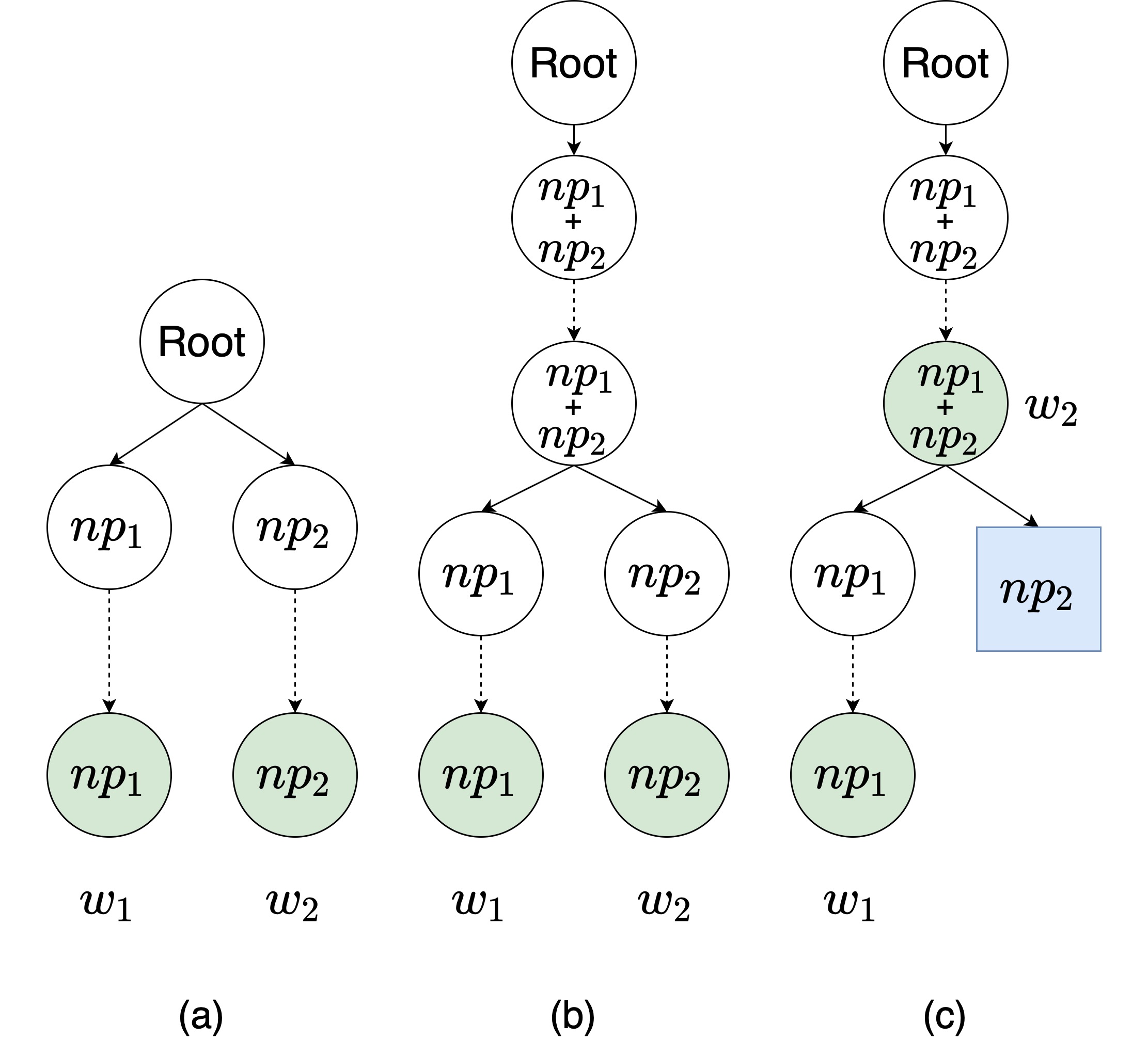
Fig. 2: Induction Base Cases

Induction: Assume that the theorem holds whenever $|\mathcal{S}|\leq k$ for some positive integer $k$. We now show that the theorem holds true for any corpus of size $k+1$. Hence assume that we are given the words $w_{1},w_{2},\ldots,w_{k+1}$ with occurence probabilities $p_{1},p_{2},\ldots p_{k+1},$ respectively.

Case I: Similar to Case I and Case II of the base case, all the words branch out at the same node together as in Fig.3. The figure also shows the expected values of the $Counter$ variables after training the Trie $n$ number of times.

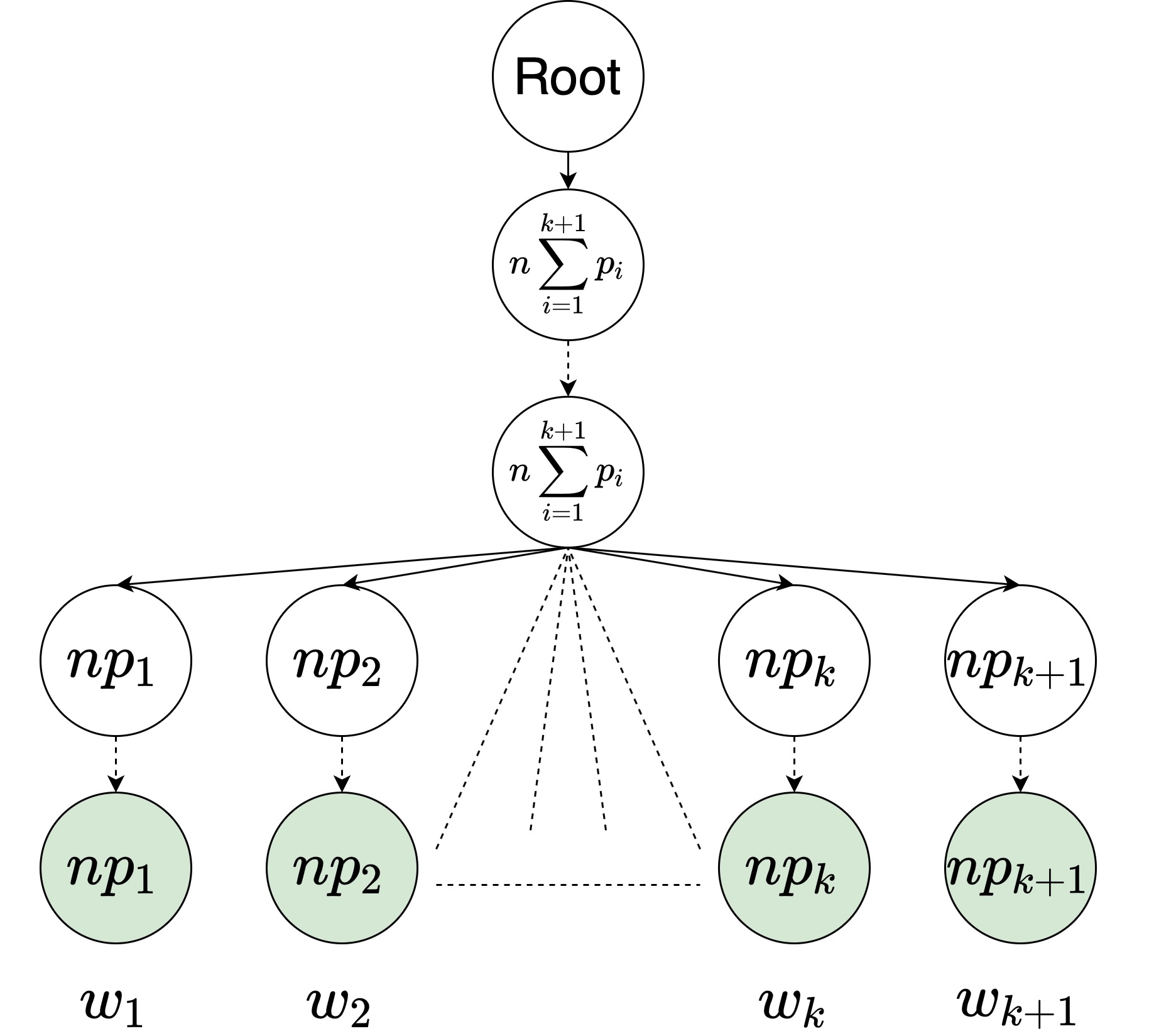
Fig. 3: Induction Step Case I

Hence we can easily conclude that for each $i=1,2,\ldots k,k+1$,

$$\mathbb{E}[\hat{p}_{i}]=\frac{np_{i}}{np_{1}+\ldots+np_{k+1}}=p_{i}\vspace{-0.1cm}$$ (6)

since $\sum_{i=1}^{k+1}{p_{i}}=1$.
Case II: In this case, consider all such possible Tries which are not covered by Case I. These Tries are in a way “more branched” than the ones considered in Case I. Consider $T$ to be any such Trie and denote its root by $R$. Notice that there must exist a subtree $T^{\prime}$, which contains strictly less than $k+1$ and at least two nodes which have their End-Of-Word set as True. It is easy to see that if not so, then $T$ lies in Case I which is a contradiction. Let us denote the root of $T^{\prime}$ by $R^{\prime}$. Let us assume that the nodes in $T^{\prime}$ for which $End-Of-Word$ is set to $True$ represent the words $w_{(1)},w_{(2)},\ldots,w_{(r)}$ with probabilities $p_{(1)},p_{(2)},\ldots,p_{(r)}$ respectively where $2\leq r<k+1$. Now suppose that $T$ instead of having the words $w_{(1)},w_{(2)},\ldots,w_{(r)}$, has a word whose characters are defined by travelling from $R$ to $R^{\prime}$ in the Trie as shown in Fig.4. Let this prefix word be $w_{\alpha}$ with a probability of $p_{\alpha}=p_{(1)}+p_{(2)}+\ldots+p_{(r)}$. Hence $T$ now practically contains strictly less than $k+1$ words. Hence by the induction hypothesis, when we train $T$, such that each one of the $k+2-r$ words is used for training at least once, the expectation of the Trie probabilities matches the occurrence probabilities. This means for each $w_{i}\in T$ whose last node doesn’t lie in $T^{\prime}$, Eqn.(6) holds true. Also, at the end of the training,

$$\mathbb{E}[Count(R^{\prime})] =n\times(p_{(1)}+p_{(2)}+\ldots+p_{(r)})$$

$$=\alpha\times\sum_{i=1}^{r}{\frac{p_{(i)}}{p_{(1)}+p_{(2)}+\ldots+p_{(r)}}}$$ (7)

where $\alpha=n\times(p_{(1)}+p_{(2)}+\ldots+p_{(r)})$. We can now consider $T^{\prime}$ to be a standalone Trie by itself, consisting of words $w_{(1)},w_{(2)},\ldots,w_{(r)}$ but truncated from the front so as to remove the characters of $w_{\alpha}$. Let these truncated words in $T^{\prime}$ be denoted by $w^{\prime}_{(1)},w^{\prime}_{(2)},\ldots,w^{\prime}_{(r)}$ with occurrence probabilities $p^{\prime}_{(1)}+p^{\prime}_{(2)}+\ldots+p^{\prime}_{(r)}$. Now notice that $T^{\prime}$ has been trained $\alpha$ number of times and since $r<k+1$, the expectation of probabilities of $T^{\prime}$ will be the same as occurrence probabilities of the truncated words which from $T$ are given by:

$$p^{\prime}_{(i)}=P_{occurrence}(w_{i}|w_{\alpha})=\frac{p_{(i)}}{p_{(1)}+p_{(2)}+\ldots+p_{(r)}}$$ (8)

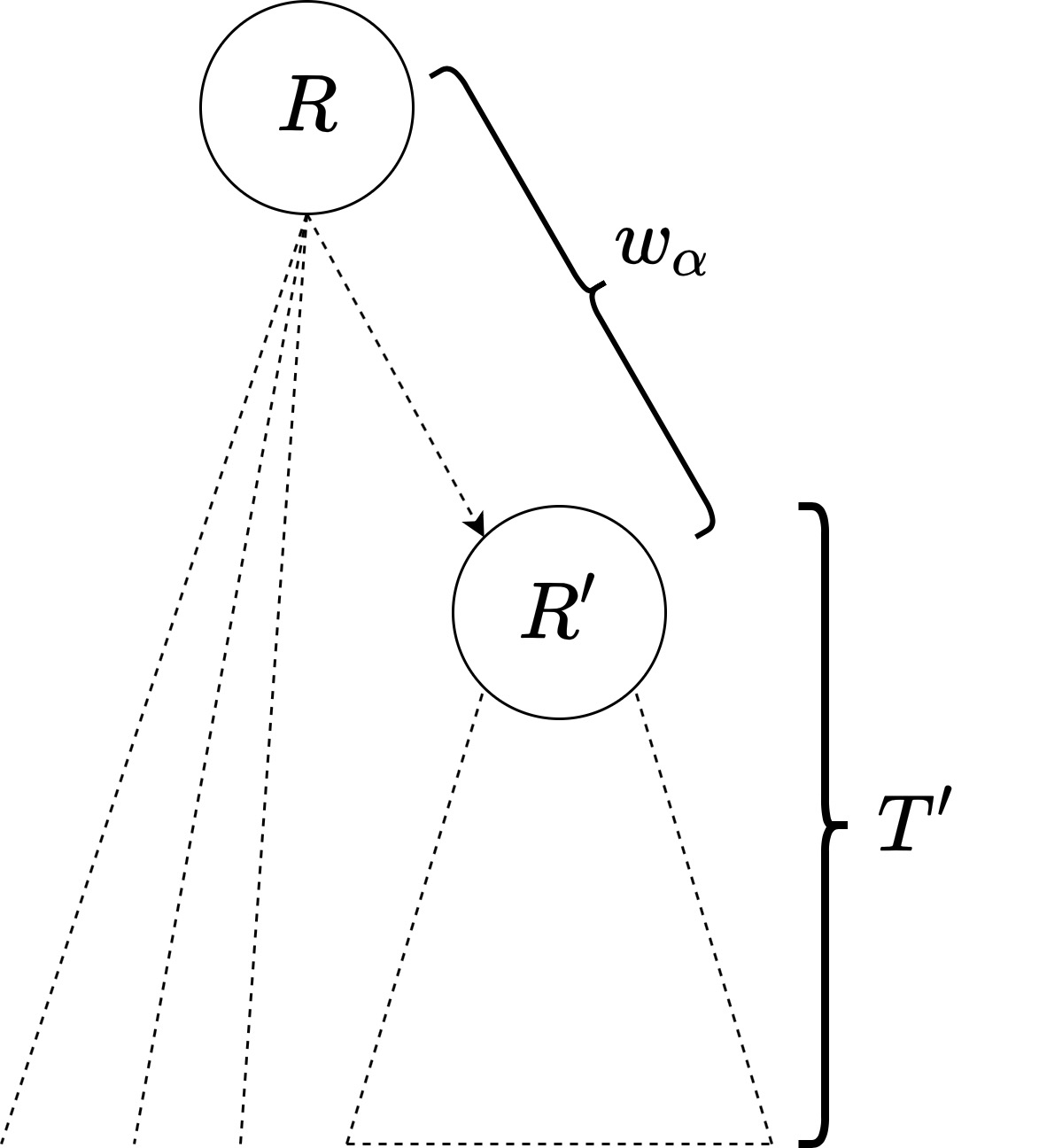
Fig. 4: Induction Step Case II

Hence, as described earlier, using induction, for each $w^{\prime}_{(i)}$, $i=1,\ldots,r$

$$\mathbb{E}[\hat{p}^{\prime}_{(i)}]=\frac{p_{(i)}}{p_{(1)}+p_{(2)}+\ldots+p_{(r)}}$$ (9)

Let us consider the entire tree $T$ with its original words $w_{(1)},w_{(2)},\ldots,w_{(r)}$ and not $w_{\alpha}$. Note that for each $w_{(i)}$, $i=1,2,\ldots,r$

$$\hat{p}_{(i)}=\hat{p}^{\prime}_{(i)}\times\hat{p}_{\alpha}$$ (10)

One may further notice that this is the same as $P_{Trie}(w_{(i)})=P_{Trie}(w_{(i)}|w_{\alpha})\times P_{Trie}(w_{\alpha})$, which implies that $\mathbb{E}[P_{Trie}(w_{(i)})]=\mathbb{E}[P_{Trie}(w_{(i)}|w_{\alpha})]\times\mathbb{E}[P_{Trie}(w_{\alpha})]$ since both of the random variables on the RHS are independent by definition. Also since $\mathbb{E}[\hat{p}_{\alpha}]=p_{(1)}+p_{(2)}+\ldots+p_{(r)}$, we can use Eqn.(9) and Eqn.(10) to get that, for each $w_{(i)}$, $i=1,\ldots,r$

$$\mathbb{E}[\hat{p}_{(i)}] =\mathbb{E}[\hat{p}^{\prime}_{(i)}]\times\mathbb{E}[\hat{p}_{\alpha}]$$

$$=\frac{p_{(i)}}{p_{(1)}+p_{(2)}+\ldots+p_{(r)}}\times(p_{(1)}+p_{(2)}+\ldots+p_{(r)})$$

$$=p_{(i)}$$

Hence for each $w_{i}\in T$, $\mathbb{E}[\hat{p}_{i}]=p_{i}$ when $|\mathcal{S}|=k+1$.


While Theorem 3.1 justifies the use of Trie through equality of occurrence probability and the expected Trie probability at any stage of training, the next theorem provides a more desired result.

Theorem 3.2: For each $w_{i}\in\mathcal{S}$, $\hat{p}_{i}\xrightarrow{a.s.}p_{i}$ as $n\rightarrow\infty$.

Proof: Let $\eta_{j}$ denote a node of the Trie such that each time any one of the words $w_{(1)},\ldots w_{(\eta_{j})}$ from $\mathcal{S}$ is sampled and used for training, its $Counter$ variable is incremented by 1. Let $W_{\eta_{j}}=\{w_{(1)},\ldots w_{(\eta_{j})}\}$.
Define, a random variable $\mathbbm{1}_{n}^{\eta_{j}}$ such that,

$$\mathbbm{1}_{n}^{\eta_{j}}=\begin{cases}1&\quad\text{if }n^{th}\text{ training word }\in W_{\eta_{j}}\\ 0&\quad\text{otherwise.}\\ \end{cases}$$

For a fixed node $\eta_{j}$, $\mathbbm{1}_{n}^{\eta_{j}}$ are i.i.d random variables for $n\in\mathbbm{N}$. Also for each $n\in\mathbbm{N}$, $\mathbb{E}[\mathbbm{1}_{n}^{\eta_{j}}]=p_{(1)}+\ldots+p_{(\eta_{j})}$. Note that the $Counter$ variable of $\eta_{j}$ is actually $\sum_{i=1}^{n}{\mathbbm{1}_{i}^{\eta_{j}}}$. Hence by using the Strong Law Of Large Numbers,

$$\frac{Counter(\eta_{j},n)}{n}=\frac{\sum_{i=1}^{n}{\mathbbm{1}_{i}^{\eta_{j}}}}{n}\xrightarrow[n\rightarrow\infty]{a.s.}p_{(1)}+\ldots+p_{(\eta_{j})}$$ (11)

With the above in mind, we proceed for induction over the number of words in $\mathcal{S}$.

Fig. 5: Base Case with Node Labels

Base Case: Let $\mathcal{S}$ contain two words $w_{1}$ and $w_{2}$ with occurrence probabilities $p_{1}$ and $p_{2}$. Then as in the previous theorem, we can get three cases which can be for our purposes be depicted by Fig.5. It is possible for $\eta_{0}$ to be the root note as well. It is also possible for exactly one of $\eta_{1}$ or $\eta_{2}$ to be a dummy node. This would cover all the three cases.
Now for $w_{1},$

$$\hat{p}_{1}= \frac{Counter(\eta_{1},n)}{Counter(\eta_{1},n)+Counter(\eta_{2},n)}$$

$$= \frac{Counter(\eta_{1},n)/n}{Counter(\eta_{1},n)/n+Counter(\eta_{2},n)/n}$$

Note that $Counter(\eta_{1},n)/n\xrightarrow[n\rightarrow\infty]{a.s.}p_{1}$ and that $Counter(\eta_{2},n)/n\xrightarrow[n\rightarrow\infty]{a.s.}p_{2}$. Hence, by using the Continuous Mapping Theorem [12], we get that

$$\hat{p}_{1}\xrightarrow[n\rightarrow\infty]{a.s.}\frac{p_{1}}{p_{1}+p_{2}}=p_{1}$$

We can similarly show that $\hat{p}_{2}\xrightarrow[n\rightarrow\infty]{a.s.}p_{2}.$ Hence our base case i.e. $|\mathcal{S}|=2$ holds true.
The proof of the induction step is similar to that of Theorem 3.1 and is being skipped due to page constraint.


From Theorem 3.1 and Theorem 3.2 we conclude that from the perspective of Theory of Estimation and using the fact that almost sure convergence is stronger than convergence in probability, we get the following corollary

Corollary 3.3: For each $w_{i}\in\mathcal{S}$, the Trie probability $\hat{p}_{i}$ is an unbiased and consistent estimator of the occurrence probability $p_{i}$.

Through the results above, we can infer that the new Trie can learn the occurrence probabilities for any set of words through sufficient training which in turn implies that the new Trie can adapt to the texting and typing style of any user when deployed on either a mobile phone, laptop or any such other device.

Fig. 6: Almost sure convergence to occurrence probabilities

4 Error Checking Algorithm

In this section, we built upon the error correction schemes used in the baseline model.

4.1 The Bayesian approach

As mentioned earlier in Section 2, in [9] the words in the suggestions list were ranked solely based on the Trie probabilities. However, following [10], we use a Bayesian noisy channel approach to rank the words based on the type of error committed by the user. This requires assignment of probabilities to the types of error for which confusion matrices in [13] can be used. Hence

$$P(w|\tilde{w})\propto P(\tilde{w}|w)P(w)$$

where $w$ denotes a possible correction for $\tilde{w}$. $P(\tilde{w}|w)$ depends on the type of error committed to get $\tilde{w}$ from $w$ and $P(w)$ is the occurrence probability of $w$ estimated using the Trie.

4.2 Character Bigram

It was observed in [9] that the Trie could generate suggestions up to a Damerau-Levenshtein distance of one. This is because generating an exhaustive list of words at a DL distance of two is computationally very expensive and is of time complexity $\mathcal{O}(26^{2M})$ where $M$ is the length of the error word. However, 80% of human errors lie within a DL distance of one and almost all within a DL distance two [14]. To partially overcome this, we propose a heuristic on the lines of beam search algorithm [15], wherein we maintain a character probability bigram denoted by $C$ where $C[i][j]$ represents the probability of the next letter being ’j’ given that the current letter is ’i’. At each stage of error correction, we provide a score to each word say $`s_{1}s_{2}\ldots s_{n}^{\prime}$ as:

$$score(word)=\Pi_{i=1}^{n-1}{C[s_{i}][s_{i+1}]}$$ (12)

and set a threshold, say $\Gamma$. If the score exceeds the threshold, the word is passed on to the next stage of error correction. This ensures that most of the intermediate low probability words are discarded while only the ones with a very high probability are passed on further.

Fig. 7: Equality of expectation to occurrence probabilites

Fig. 8: Performance comparison of the two TRIE based models

5 Simulations

5.1 Almost sure convergence

In light of Theorem 3.2, a simulation was performed where we trained the new Trie using the training and probability generation algorithms defined in Section 3 with the eight words used in Section 2. The Trie probabilities denoted by the bold lines evidently converge to the occurrence probabilities denoted by the dotted lines in Fig.6.

5.2 Equality of expectation

Similar to the simulation done in Section 5.1, we train 30 Tries and take the average of their probabilities. The bold lines can be seen to converge much faster to the dotted lines in Fig.7 than in Fig.6. This supports the theorem stating the equality of expectation of the Trie probabilities to the occurrence probabilities.

5.3 Comparison

In this simulation, we consecutively train both, the new Trie model proposed by us and the baseline Trie model using a corpus of twenty words. The assigned occurrence probabilities to these words are depicted in Fig.8. The new Trie clearly outperforms the one proposed baseline Trie. An important observation is that the baseline Trie probabilities clearly sum up to more than one, hence not a valid probability measure.

5.4 Error correction

We use a corpus of 3000 highest frequency English words and use Zipf’s Law to fit a probability distribution over the ranked data. Comparative analysis with the baseline shown in Table 1 clearly showcases superiority of the new model.

Table 1: Comparison of output with baseline Trie

Impure	Target	Top 5 Suggestions	Rank	Rank in [9]
tran	train	than, train , ran, trap, tan	2	5
lng	long	long, lang, log, leg, an, gang	1	4
aple	apple	pale, alle, able, apple, ample	4	5
beleive	believe	believe, believed, believes	1	1
gost	ghost	host, lost, most, past, ghost	5	1
moble	noble	noble, nobler, nobles	1	2
cuz	cause	use, case, cause, cut, cup	3	8
cin	seen	in, can, sin, son, skin	13	17
dem	them	them, then, den, chem, the	1	11
m8	mate	mate, might, eight, ate, mare	1	6
thx	thanks	the, thy, tax, thanks, them	4	1
h8	hate	hate, height, hare, ate, haste	1	-

6 Conclusions

In the paper, we first pointed out a a limitation in the Trie based probability generating model proposed in existing literature, to overcome which, we proposed a structural modification, a training algorithm and a probability generating scheme. We further proved rigorously that the new Trie generated probabilities are an unbiased and consistent estimator of the occurrence probabilities. These occurrence probabilities vary user to user which the new Trie is capable of adapting to. We performed simulations, the results of which strongly support both the presented theorems and demonstrated superiority in error correction.

References

- Crystal [2006] David Crystal. Language and the Internet. Cambridge University Press, 2 edition, 2006.
- Jurafsky and Martin [2009] Daniel Jurafsky and James H. Martin. Speech and Language Processing (2nd Edition). Prentice-Hall, Inc., USA, 2009.
- Kobus et al. [2008] Catherine Kobus, François Yvon, and Géraldine Damnati. Normalizing sms: are two metaphors better than one ? In COLING, 2008.
- Li and Liu [2012] Chen Li and Yang Liu. Normalization of text messages using character- and phone-based machine translation approaches. In INTERSPEECH, 2012.
- Desai and Narvekar [2015] Neelmay Desai and Meera Narvekar. Normalization of noisy text data. Procedia Computer Science, 45, 12 2015.
- Khan and Karim [2012] O. A. Khan and A. Karim. A rule-based model for normalization of sms text. In 2012 IEEE 24th International Conference on Tools with Artificial Intelligence, volume 1, pages 634–641, 2012.
- Veliz et al. [2019] Claudia Matos Veliz, Orphée De Clercq, and Véronique Hoste. Comparing mt approaches for text normalization. In RANLP, 2019.
- Choudhury et al. [2007] Monojit Choudhury, Rahul Saraf, Vijit Jain, Animesh Mukherjee, Sudeshna Sarkar, and Basu Anupam. Investigation and modeling of the structure of texting language. IJDAR, 10:157–174, 12 2007.
- Chatterjee [2019] Niladri Chatterjee. A Trie Based Model for SMS Text Normalization, pages 846–859. 06 2019.
- Keyboards and Kirk [2019] Keyboards and Amanda Kirk. Improving the accuracy of mobile touchscreen qwerty. 2019.
- Grinter and Eldridge [2001] Rebecca E. Grinter and Margery A. Eldridge. y do tngrs luv 2 txt msg?, pages 219–238. Springer Netherlands, Dordrecht, 2001.
- van der Vaart [2000] A.W. van der Vaart. Asymptotic Statistics. Asymptotic Statistics. Cambridge University Press, 2000.
- Kernighan et al. [1990] Mark Kernighan, Kenneth Church, and William Gale. A spelling correction program based on a noisy channel model. pages 205–210, 01 1990.
- Damerau [1964] Fred J. Damerau. A technique for computer detection and correction of spelling errors. Commun. ACM, 7(3):171–176, March 1964.
- 659 [1977] Speech understanding systems. IEEE Transactions on Professional Communication, PC-20(4):221–225, 1977.