Faster Stochastic Alternating Direction Method of Multipliers
for Nonconvex Optimization

Abstract

In this paper, we propose a faster stochastic alternating direction method of multipliers (ADMM) for nonconvex optimization by using a new stochastic path-integrated differential estimator (SPIDER), called as SPIDER-ADMM. Moreover, we prove that the SPIDER-ADMM achieves a record-breaking incremental first-order oracle (IFO) complexity of $\mathcal{O}(n+n^{1/2}\epsilon^{-1})$ for finding an $\epsilon$-approximate stationary point, which improves the deterministic ADMM by a factor $\mathcal{O}(n^{1/2})$, where $n$ denotes the sample size. As one of major contribution of this paper, we provide a new theoretical analysis framework for nonconvex stochastic ADMM methods with providing the optimal IFO complexity. Based on this new analysis framework, we study the unsolved optimal IFO complexity of the existing non-convex SVRG-ADMM and SAGA-ADMM methods, and prove they have the optimal IFO complexity of $\mathcal{O}(n+n^{2/3}\epsilon^{-1})$. Thus, the SPIDER-ADMM improves the existing stochastic ADMM methods by a factor of $\mathcal{O}(n^{1/6})$. Moreover, we extend SPIDER-ADMM to the online setting, and propose a faster online SPIDER-ADMM. Our theoretical analysis shows that the online SPIDER-ADMM has the IFO complexity of $\mathcal{O}(\epsilon^{-\frac{3}{2}})$, which improves the existing best results by a factor of $\mathcal{O}(\epsilon^{-\frac{1}{2}})$. Finally, the experimental results on benchmark datasets validate that the proposed algorithms have faster convergence rate than the existing ADMM algorithms for nonconvex optimization.

1 Introduction

Alternating direction method of multipliers (ADMM) (Gabay & Mercier, 1976; Boyd et al., 2011) is a powerful optimization tool for the composite or constrained problems in machine learning. In general, it considers the following optimization problem:

$$\min_{x,y}f(x)+g(y),\quad\mbox{s.t.}\ Ax+By=c,\vspace*{-4pt}$$

where $f(x):\mathbb{R}^{d}\rightarrow\mathbb{R}$ and $g(y):\mathbb{R}^{p}\rightarrow\mathbb{R}$ are convex functions. For example, in machine learning, $f(x)$ can be used for the empirical loss, $g(y)$ for the structure regularizer, and the constraint for encoding the structure pattern of model parameters. Due to the flexibility in splitting the objective function into loss $f(x)$ and regularizer $g(y)$, the ADMM can relatively easily solve some complicated structure problems in machine learning, such as the graph-guided fused lasso (Kim et al., 2009) and the overlapping group lasso, which are too complicated for the other popular optimization methods such as proximal gradient methods (Nesterov, 2005; Beck & Teboulle, 2009). Thus, the ADMM has been extensively studied in recent years (Boyd et al., 2011; Nishihara et al., 2015; Xu et al., 2017).

The above deterministic ADMM generally needs to compute the gradients of empirical loss function on all examples at each iteration, which makes it unsuitable for solving big data problems. Thus, the online and stochastic versions of ADMM (Wang & Banerjee, 2012; Suzuki, 2013; Ouyang et al., 2013) are developed. However, due to large variance of stochastic gradients, these stochastic methods suffer from a slow convergence rate. Recently, some fast stochastic ADMM methods (Zhong & Kwok, 2014; Suzuki, 2014; Zheng & Kwok, 2016a) have been proposed by using the variance reduced (VR) techniques.

Table 1: IFO complexity comparison of the non-convex ADMM methods for finding an $\epsilon$-approximate stationary point of the problem (1), i.e., $\mathbb{E}\|\nabla\mathcal{L}(x,y_{[m]},z)\|^{2}\leq\epsilon$. $n$ denotes the sample size.

Problem	Algorithm	Reference	IFO
Finite-sum	ADMM	Jiang et al. (2019)	$\mathcal{O}(n\epsilon^{-1})$
	SVRG-ADMM	Huang et al. (2016); Zheng & Kwok (2016b)	$\mathcal{O}(n+n^{\frac{2}{3}}\epsilon^{-1})$
	SAGA-ADMM	Huang et al. (2016)	$\mathcal{O}(n+n^{\frac{2}{3}}\epsilon^{-1})$
	SPIDER-ADMM	Ours	$\mathcal{O}(n+n^{\frac{1}{2}}\epsilon^{-1})$
Online	SADMM	Huang & Chen (2018)	$\mathcal{O}(\epsilon^{-2})$
	Online SPIDER-ADMM	Ours	$\mathcal{O}(\epsilon^{-\frac{3}{2}})$

So far, the above discussed ADMM methods build on the convexity of objective functions. In fact, ADMM is also highly successful in solving various nonconvex problems such as tensor decomposition (Kolda & Bader, 2009) and training neural networks (Taylor et al., 2016). Thus, some works (Li & Pong, 2015; Wang et al., 2015a, b; Hong et al., 2016; Jiang et al., 2019) have devoted to studying the non-convex ADMM methods. More recently, for solving the big data problems, the nonconvex stochastic ADMMs (Huang et al., 2016; Zheng & Kwok, 2016b) have been proposed with the VR techniques such as the SVRG (Johnson & Zhang, 2013) and the SAGA (Defazio et al., 2014). In addition, Huang & Chen (2018) have extended the online/stochastic ADMM (Ouyang et al., 2013) to the nonconvex setting.

Although these works have studied the convergence of nonconvex stochastic ADMMs and proved these methods have $\mathcal{O}(\frac{c}{T})$ convergence rate, where $T$ denotes number of iteration and $c$ a constant independent on $T$, they have not provided the optimal incremental/stochastic first-order oracle (IFO/SFO (Ghadimi & Lan, 2013)) complexity for these methods yet. In other words, they have only proved these stochastic ADMMs have the same convergence rate to the deterministic ADMM (Jiang et al., 2019), but don’t tell us whether these stochastic ADMMs have less IFO complexity than the deterministic ADMM, which is a key assessment criteria of the first-order stochastic methods (Reddi et al., 2016). For example, from the existing noncovex SAGA-ADMM and SVRG-ADMM (Zheng & Kwok, 2016b; Huang et al., 2016), we only obtain a rough IFO complexity of $\mathcal{O}(n+bc\epsilon^{-1})$ for finding an $\epsilon$-approximate stationary point, where $b$ denotes the mini-batch size. In their convergence analysis, to ensure the convergence of these methods, they need to choose a small step size $\eta$ and a large penalty parameter $\rho$. Under this case, we maybe have $bc\geq n$, so that these stochastic ADMMs have no less IFO complexity than the deterministic ADMM. Thus, there still exist two important problems to be addressed:

• Does the stochastic ADMM have less IFO complexity than the deterministic ADMM for nonconvex optimization?

• If the stochastic ADMM improves IFO complexity, how much can it improve?

In the paper, we answer the above challenging questions with positive solutions and propose a new faster stochastic ADMM method (i.e., SPIDER-ADMM) to solve the following nonconvex nonsmooth problem:

$$\min_{x,\{y_{j}\}_{j=1}^{m}} f(x):=\left\{\begin{aligned} &\frac{1}{n}\sum_{i=1}^{n}f_{i}(x)\ \mbox{(finite-sum)}\\ &\mathbb{E}_{\zeta}[f(x;\zeta)]\ \mbox{(online)}\end{aligned}\right.+\sum_{j=1}^{m}g_{j}(y_{j})$$

s.t. $$\quad Ax+\sum_{j=1}^{m}B_{j}y_{j}=c,$$ (1)

where $A\in\mathbb{R}^{l\times d}$, $B_{j}\in\mathbb{R}^{l\times p}$ for all $j\in[m]$, and $\zeta$ is a random variable following an unknown distribution. Here $f(x):\mathbb{R}^{d}\rightarrow\mathbb{R}$ is a nonconvex and smooth function, and $g_{j}(y_{j}):\mathbb{R}^{p}\rightarrow\mathbb{R}$ is a convex and possibly nonsmooth function for all $j\in[m],\ m\geq 1$. In machine learning, $f(x)$ can be used for losses such as activation functions of neural networks, $\sum_{j=1}^{m}g_{j}(y_{j})$ can be used for not only single structure penalty (e.g., sparse, low rank) but also superposition structures penalties (e.g., sparse + low rank, sparse + group sparse), which are widely applied in robust PCA (Candès et al., 2011), subspace clustering (Liu et al., 2010), and dirty models (Jalali et al., 2010). For the problem (1), its finite-sum subproblem generally arises from the empirical loss minimization and M-estimation. While its online subproblem comes from the expected loss minimization. To address the online subproblem, we extend the SPIDER-ADMM to the online setting, and propose an online SPIDER-ADMM.

Challenges and Contributions

Our SPIDER-ADMM methods build on the variance-reduced technique of SPIDER (Fang et al., 2018) and SpiderBoost (Wang et al., 2018), which is a variant of stochastic recursive gradient algorithm (SARAH (Nguyen et al., 2017a, b)) and reaches the state-of-the-art IFO complexity as the SNVRG (Zhou et al., 2018). Although the SPIDER and SpiderBoost have shown good performances in the stochastic gradient descent (SGD) and proximal SGD methods, applying these techniques to the nonconvex ADMM method is not a trivial task. There exist the following two main challenges:

• Due to failure of the Fejér monotonicity of iteration, the convergence analysis of the nonconvex ADMM is generally quite difficult (Wang et al., 2015a). With using the inexact stochastic gradient, this difficulty is greater in the nonconvex stochastic ADMM methods;

• To obtain the optimal IFO complexity of our methods, we need to design a new effective Lyapunov function, which can not follow the existing nonconvex stochastic ADMM methods (Huang et al., 2016).

In this paper, thus, we will fill this gap between the nonconvex ADMM and the SPIDER/SpiderBoost methods. Our main contributions are summarized as follows:

• We propose a faster stochastic ADMM ( i.e., SPIDER-ADMM ) method for nonconvex optimization based on the SPIDER/SpiderBoost. Moreover, we prove that the SPIDER-ADMM achieves a lower IFO complexity of $\mathcal{O}(n+n^{1/2}\epsilon^{-1})$ for finding an $\epsilon$-approximate stationary point, which improves the deterministic ADMM by a factor $\mathcal{O}(n^{1/2})$.

• We extend the SPIDER-ADMM method to the online setting, and propose a faster online SPIDER-ADMM for nonconvex optimization. Moreover, we prove that the online SPIDER-ADMM achieves a lower IFO complexity of $\mathcal{O}(\epsilon^{-\frac{3}{2}})$, which improves the existing best results by a factor of $\mathcal{O}(\epsilon^{-\frac{1}{2}})$.

• We provide a useful theoretical analysis framework for nonconvex stochastic ADMM methods with providing the optimal IFO complexity. Based on our new analysis framework, we also prove that the existing nonconvex SVRG-ADMM and SAGA-ADMM have the optimal IFO complexity of $\mathcal{O}(n+n^{2/3}\epsilon^{-1})$. Thus, our SPIDER-ADMM improves the existing stochastic ADMMs by a factor of $\mathcal{O}(n^{1/6})$.

Notations

Let $y_{[m]}=\{y_{1},\cdots,y_{m}\}$ and $y_{[j:m]}=\{y_{j},\cdots,y_{m}\}$ for $j\in[m]=\{1,2,\cdots,m\}$. Given a positive definite matrix $G$, $\|x\|^{2}_{G}=x^{T}Gx$; $\sigma_{\max}(G)$ and $\sigma_{\min}(G)$ denote the largest and smallest eigenvalues of matrix $G$, respectively; $\kappa_{G}=\frac{\sigma_{\max}(G)}{\sigma_{\min}(G)}\geq 1$. $\sigma^{A}_{\max}$ and $\sigma^{A}_{\min}$ denote the largest and smallest eigenvalues of matrix $A^{T}A$, respectively. Given positive definite matrices $\{H_{j}\}_{j=1}^{m}$, let $\sigma^{H}_{\min}=\min_{j}\sigma_{\min}(H_{j})$ and $\sigma^{H}_{\max}=\max_{j}\sigma_{\max}(H_{j})$. $I_{d}$ denotes a $d\times d$ identity matrix.

2 Preliminaries

In the section, we introduce some preliminaries regarding problem (1). First, we restate the standard $\epsilon$-approximate stationary point of the nonconvex problem (1) used in (Jiang et al., 2019; Zheng & Kwok, 2016b).

Definition 1.

Given $\epsilon>0$, the point $(x^{*},y_{[m]}^{*},z^{*})$ is said to be an $\epsilon$-stationary point of the problem (1), if it holds that

$$\mathbb{E}\big{[}\mbox{dist}(0,\partial L(x^{*},y^{*}_{[m]},z^{*}))^{2}\big{]}\leq\epsilon,$$ (2)

where $L(x,y_{[m]},z)=f(x)+\sum_{j=1}^{m}g_{j}(y_{j})-\langle z,Ax+\sum_{j=1}^{m}B_{j}y_{j}-c\rangle$,

$$\partial L(x,y_{[m]},z)=\left[\begin{matrix}\nabla_{x}L(x,y_{[m]},z)\\ \partial_{y_{1}}L(x,y_{[m]},z)\\ \cdots\\ \partial_{y_{m}}L(x,y_{[m]},z)\\ -Ax-\sum_{j=1}^{m}B_{j}y_{j}+c\end{matrix}\right],$$

and $\mbox{dist}(0,\partial L)=\inf_{L^{\prime}\in\partial L}\|0-L^{\prime}\|.$

Next, we give some standard assumptions regarding problem (1) as follows:

Assumption 1.

Each loss function $f_{i}(x)$ is $L$-smooth such that

$$\|\nabla f_{i}(x)-\nabla f_{i}(y)\|\leq L\|x-y\|,\ \forall x,y\in\mathbb{R}^{d},$$

which is equivalent to

$$f_{i}(x)\leq f_{i}(y)+\nabla f_{i}(y)^{T}(x-y)+\frac{L}{2}\|x-y\|^{2}.$$

Assumption 2.

Full gradient of loss function $f(x)$ is bounded, i.e., there exists a constant $\delta>0$ such that for all $x$, it follows $\|\nabla f(x)\|^{2}\leq\delta^{2}$.

Assumption 3.

$f(x)$ and $g_{j}(y_{j})$ for all $j\in[m]$ are all lower bounded, and let $f^{*}=\inf_{x}f(x)>-\infty$ and $g_{j}^{*}=\inf_{y_{j}}g_{j}(y_{j})>-\infty$.

Assumption 4.

$A$ is a full row or column rank matrix.

Assumption 1 imposes smoothness on the individual loss functions, which is commonly used in convergence analysis of the nonconvex algorithms (Ghadimi & Lan, 2013; Ghadimi et al., 2016). Assumption 2 shows full gradient of loss function have a bounded norm, which is used in the stochastic gradient-based and ADMM-type methods (Boyd et al., 2011; Suzuki, 2013; Hazan et al., 2016). Assumptions 3 and 4 have been used in the study of nonconvex ADMMs (Hong et al., 2016; Jiang et al., 2019; Zheng & Kwok, 2016b). Assumptions 3 guarantees the feasibility of the problem (1). Assumption 4 guarantees the matrix $A^{T}A$ or $AA^{T}$ is non-singular. Since there exist multiple regularizers in the above problem (1), $A$ is general a full column rank matrix. Without loss of generality, we will use the full column rank matrix $A$ below.

3 Fast SPIDER-ADMM Method

In the section, we propose a new faster stochastic ADMM algorithm, i.e., SPIDER-ADMM, to solve the finite-sum problem (1). We begin with giving the augmented Lagrangian function of the problem (1):

$$\mathcal{L}_{\rho}(x,y_{[m]},z)= f(x)+\sum_{j=1}^{m}g_{j}(y_{j})-\langle z,Ax+\sum_{j=1}^{m}B_{j}y_{j}-c\rangle$$

$$+\frac{\rho}{2}\|Ax+\sum_{j=1}^{m}B_{j}y_{j}-c\|^{2},$$ (3)

where $z\in\mathbb{R}^{l}$ and $\rho>0$ denote the dual variable and penalty parameter, respectively. Algorithm 1 gives the SPIDER-ADMM algorithmic framework.

In Algorithm 1, we use the proximal method to update the variables $\{y_{j}\}_{j=1}^{m}$. At the step 9 of Algorithm 1, we update the variables $\{y_{j}\}_{j=1}^{m}$ by solving the following subproblem, for all $j\in[m]$

$$y^{k+1}_{j}\!=\!\mathop{\arg\min}_{y_{j}\in\mathbb{R}^{p}}\mathcal{L}_{\rho}(x_{k},y^{k+1}_{[j-1]},y_{j},y^{k}_{[j+1:m]},z_{k})\!+\!\frac{1}{2}\|y_{j}\!-\!y^{k}_{j}\|_{H_{j}}^{2},$$

where

$$\mathcal{L}_{\rho}(x_{k},y^{k+1}_{[j-1]},y_{j},y^{k}_{[j+1:m]},z_{k})=f(x_{k})+\sum_{i=1}^{j-1}g_{i}(y^{k+1}_{i})$$

$$+g_{j}(y_{j})\!+\!\sum_{i=j+1}^{m}g_{j}(y^{k}_{j})\!-\!z_{k}^{T}(B_{j}y_{j}+\tilde{c})\!+\!\frac{\rho}{2}\|B_{j}y_{j}+\tilde{c}\|^{2}\vspace*{-6pt}$$

with $\tilde{c}=Ax_{k}+\sum_{i=1}^{j-1}B_{i}y_{i}^{k+1}+\sum_{i=j+1}^{m}B_{i}y_{i}^{k}-c$ and $H_{j}\succ 0$. When set $H_{j}=r_{j}I_{p}-\rho B_{j}^{T}B_{j}\succeq I_{p}$ with $r_{j}\geq\rho\sigma_{\max}(B^{T}_{j}B_{j})+1$ for all $j\in[m]$ to linearize the term $\frac{\rho}{2}\|B_{j}y_{j}+\tilde{c}\|^{2}$, then we can use the following proximal operator to update $y_{j}$, for all $j\in[m]$

$$y^{k+1}_{j}=\mathop{\arg\min}_{y_{j}\in\mathbb{R}^{p}}\frac{r_{j}}{2}\|y_{j}-w^{k}_{j}\|^{2}+g_{j}(y_{j}),$$ (4)

where $w^{k}_{j}=\frac{1}{r_{j}}\big{(}H_{j}y^{k}_{j}-\rho B^{T}_{j}\tilde{c}+B^{T}_{j}z_{k}\big{)}$.

To update $x$, we define an approximated function over $x_{k}$ as follows:

$$\hat{\mathcal{L}}_{\rho}(x,y^{k+1}_{[m]},z_{k},v_{k})=f(x_{k})+v_{k}^{T}(x-x_{k})+\frac{1}{2\eta}\|x-x_{k}\|^{2}_{G}$$

$$+\sum_{j=1}^{m}g_{j}(y^{k+1}_{j})-z_{k}^{T}(Ax+\sum_{j=1}^{m}B_{j}y^{k+1}_{j}-c)$$

$$+\frac{\rho}{2}\|Ax+\sum_{j=1}^{m}B_{j}y_{j}^{k+1}-c\|^{2},$$ (5)

where $\eta>0$ is a step size; $v_{k}$ is a stochastic gradient over $x_{k}$; $G\succ 0$ is a positive matrix. In updating $x$, to avoid computing inverse of $\frac{G}{\eta}+\rho A^{T}A$, we can set $G=rI_{d}-\rho\eta A^{T}A\succeq I_{d}$ with $r\geq\rho\eta\sigma^{A}_{\max}+1$ to linearize term $\frac{\rho}{2}\|Ax+\sum_{j=1}^{m}B_{j}y^{k+1}_{j}-c\|^{2}$. Then at the step 10 of Algorithm 1, we have

$$x_{k+1}=\frac{Gx_{k}}{r}-\frac{\eta v_{k}}{r}-\frac{\eta\rho}{r}A^{T}(\sum_{j=1}^{m}B_{j}y_{j}^{k+1}-c-\frac{z_{k}}{\rho}).$$

In Algorithm 1, after setting $v_{0}=\nabla f(x_{0})$, for each subsequent iteration $k$, we have:

$$v_{k}=\nabla f_{\mathcal{I}_{k}}(x_{k})-\nabla f_{\mathcal{I}_{k}}(x_{k-1})+v_{k-1},$$ (6)

where $\nabla f_{\mathcal{I}_{k}}(x_{k})=\frac{1}{|\mathcal{I}_{k}|}\sum_{i\in\mathcal{I}_{k}}\nabla f_{i}(x_{t})$. It is easy to check $\mathbb{E}[v_{k}|x_{0}]=\nabla f(x_{k})$, i.e., an unbiased estimate gradient over $x_{k}$. Comparing the existing SVRG-ADMM, our SPIDER-ADMM constructs stochastic gradient $v_{k}$ based on the information $x_{k-1}$ and $v_{k-1}$, while the SVRG-ADMM constructs $v_{k}$ based on the information $x_{0}$ and $v_{0}$ (i.e., the initalization information of each outer loop). Due to using more fresh information, thus, SPIDER-ADMM can yield more accurate estimation of the full gradient than SVRG-ADMM. Simultaneously, it does not require to additional computation and memory, so it costs less memory than the existing SAGA-ADMM.

Algorithm 1 SPIDER-ADMM Algorithm

1:  Input: $b$, $q$, $K$, $\eta>0$ and $\rho>0$;

2:  Initialize: $x_{0}\in\mathbb{R}^{d}$, $y^{0}_{j}\in\mathbb{R}^{p},\ j\in[m]$ and $z_{0}\in\mathbb{R}^{l}$;

3:  for $k=0,1,\cdots,K-1$ do

4:     if $\mbox{mod}(k,q)=0$ then

5:         Compute $v_{k}=\nabla f(x_{k})$;

6:     else

7:         Uniformly randomly pick a mini-batch $\mathcal{I}_{k}$ (with replacement) from $\{1,2,\cdots,n\}$ with $|\mathcal{I}_{k}|=b$, and compute

$$v_{k}=\nabla f_{\mathcal{I}_{k}}(x_{k})-\nabla f_{\mathcal{I}_{k}}(x_{k-1})+v_{k-1};$$

8:     end if

9:      $y^{k+1}_{j}=\arg\min_{y_{j}}\big{\{}\mathcal{L}_{\rho}(x_{k},y^{k+1}_{[j-1]},y_{j},y^{k}_{[j+1:m]},z_{k})+\frac{1}{2}\|y_{j}-y^{k}_{j}\|_{H_{j}}^{2}\big{\}}$ for all $j\in[m]$;

10:      $x_{k+1}=\arg\min_{x}\hat{\mathcal{L}}_{\rho}\big{(}x,y^{k+1}_{[m]},z_{k},v_{k}\big{)}$;

11:      $z_{k+1}=z_{k}-\rho(Ax_{k+1}+\sum_{j=1}^{m}B_{j}y^{k+1}_{j}-c)$;

12:  end for

13:  Output  (in theory): Chosen uniformly random from $\{x_{k},y_{[m]}^{k},z_{k}\}_{k=1}^{K}$.

14:  Output  (in practice): $\{x_{K},y_{[m]}^{K},z_{K}\}$.

4 Fast Online SPIDER-ADMM Method

In the section, we propose an online SPIDER-ADMM to solve the online problem (1), which is equivalent to the following stochastic constrained problem:

$$\min_{x,\{y_{j}\}_{j=1}^{m}} \mathbb{E}_{\zeta}[f(x;\zeta)]+\sum_{j=1}^{m}g_{j}(y_{j}),$$

s.t. $$\ Ax+\sum_{j=1}^{m}B_{j}y_{j}=c,$$ (7)

where $f(x)=\mathbb{E}_{\zeta}[f(x;\zeta)]$ denotes a population risk over an underlying data distribution. The problem (4) can be viewed as having infinite samples, so we cannot evaluate the full gradient $\nabla f(x)$. For solving the problem (4), so we use stochastic sampling to evaluate the full gradient. Algorithm 2 shows the algorithmic framework of online SPIDER-ADMM method. In Algorithm 2, we use the mini-batch samples to estimate the full gradient, and update the variables $\{x,y_{j},z\}_{j=1}^{m}$, which is the same as in Algorithm 1.

Algorithm 2 Online SPIDER-ADMM Algorithm

1:  Input: $b_{1}$, $b_{2}$, $q$, $K$, $\eta>0$ and $\rho>0$;

2:  Initialize: $x_{0}\in\mathbb{R}^{d}$, $y^{0}_{j}\in\mathbb{R}^{p},\ j\in[m]$ and $z_{0}\in\mathbb{R}^{l}$;

3:  for $k=0,1,\cdots,K-1$ do

4:     if $\mbox{mod}(k,q)=0$ then

5:         Draw $S_{1}$ samples with $|S_{1}|=b_{1}$, and compute $v_{k}=\frac{1}{b_{1}}\sum_{i\in S_{1}}\nabla f_{i}(x_{k})$;

6:     else

7:         Draw $S_{2}$ samples with $|S_{2}|=b_{2}=\sqrt{b_{1}}$, and compute

$$v_{k}=\frac{1}{b_{2}}\sum_{i\in S_{2}}\big{(}\nabla f_{i}(x_{k})-f_{i}(x_{k-1})\big{)}+v_{k-1};$$

8:     end if

9:      $y^{k+1}_{j}=\arg\min_{y_{j}}\big{\{}\mathcal{L}_{\rho}(x_{k},y^{k+1}_{[j-1]},y_{j},y^{k}_{[j+1:m]},z_{k})+\frac{1}{2}\|y_{j}-y^{k}_{j}\|_{H_{j}}^{2}\big{\}}$ for all $j\in[m]$;

10:      $x_{k+1}=\arg\min_{x}\hat{\mathcal{L}}_{\rho}\big{(}x,y^{k+1}_{[m]},z_{k},v_{k}\big{)}$;

11:      $z_{k+1}=z_{k}-\rho(Ax_{k+1}+\sum_{j=1}^{m}B_{j}y^{k+1}_{j}-c)$;

12:  end for

13:  Output  (in theory): Chosen uniformly random from $\{x_{k},y_{[m]}^{k},z_{k}\}_{k=1}^{K}$.

14:  Output  (in practice): $\{x_{K},y_{[m]}^{K},z_{K}\}$.

5 Convergence Analysis

In the section, we study the convergence properties of both the SPIDER-ADMM and online SPIDER-ADMM. At the same time, based on our new theoretical analysis framework, we afresh analyze the convergence properties of existing ADMM-based nonconvex optimization algorithms, i.e., SVRG-ADMM and SAGA-ADMM, and derive their optimal IFO complexity for finding an $\epsilon$-approximate stationary point.

5.1 Convergence Analysis of SPIDER-ADMM

In the subsection, we study convergence properties of the SPIDER-ADMM algorithm. The detailed proofs are provided in the Appendix A.1. Throughout the paper, let $n_{k}=\lceil k/q\rceil$ such that $(n_{k}-1)q\leq k\leq n_{k}q-1$.

Lemma 1.

Suppose the sequence $\{x_{k},y_{[m]}^{k},z_{k}\}_{k=1}^{K}$ is generated from Algorithm 1, and define a Lyapunov function $R_{k}$ as follows:

$$R_{k}\!=\! \mathcal{L}_{\rho}(x_{k},y_{[m]}^{k},z_{k})\!+\!(\frac{9L^{2}}{\sigma^{A}_{\min}\rho}\!+\!\frac{3\sigma^{2}_{\max}(G)}{\sigma^{A}_{\min}\eta^{2}\rho})\|x_{k}\!-\!x_{k-1}\|^{2}$$

$$\!+\!\frac{2L^{2}}{\sigma^{A}_{\min}\rho b}\sum_{i=(n_{k}-1)q}^{k-1}\mathbb{E}\|x_{i+1}\!-\!x_{i}\|^{2}.$$

Let $b=q$, $\eta=\frac{2\alpha\sigma_{\min}(G)}{3L}\ (0<\alpha\leq 1)$ and $\rho=\frac{\sqrt{170}\kappa_{G}L}{\sigma^{A}_{\min}\alpha}$, then we have

$$\frac{1}{K}\sum_{k=0}^{K-1}\big{(}\|x_{k+1}-x_{k}\|^{2}+\sum_{j=1}^{m}\|y_{j}^{k}-y_{j}^{k+1}\|^{2}\big{)}\leq\frac{R_{0}-R^{*}}{K\gamma},$$

where $\gamma=\min(\chi,\sigma_{\min}^{H})$ with $\chi\geq\frac{\sqrt{170}\kappa_{G}L}{4\alpha}$ and $R^{*}$ is a lower bound of the function $R_{k}$.

Let $\theta_{k}=\mathbb{E}[\|x_{k+1}-x_{k}\|^{2}+\|x_{k}-x_{k-1}\|^{2}+\frac{1}{q}\sum_{i=(n_{k}-1)q}^{k}\|x_{i+1}-x_{i}\|^{2}+\sum_{j=1}^{m}\|y_{j}^{k}-y_{j}^{k+1}\|^{2}]$. Next, based on the above lemma, we give the convergence properties of SPIDER-ADMM.

Theorem 1.

Suppose the sequence $\{x_{k},y_{[m]}^{k},z_{k})_{k=1}^{K}$ is generated from Algorithm 1. Let

$$\nu_{1}=m\big{(}\rho^{2}\sigma^{B}_{\max}\sigma^{A}_{\max}+\rho^{2}(\sigma^{B}_{\max})^{2}+\sigma^{2}_{\max}(H)\big{)},$$

$$\nu_{2}=3(L^{2}+\frac{\sigma^{2}_{\max}(G)}{\eta^{2}}),\nu_{3}=\frac{18L^{2}}{\sigma^{A}_{\min}\rho^{2}}+\frac{3\sigma^{2}_{\max}(G)}{\sigma^{A}_{\min}\eta^{2}\rho^{2}},$$

and let $b=q$, $\eta=\frac{2\alpha\sigma_{\min}(G)}{3L}\ (0<\alpha\leq 1)$, and $\rho=\frac{\sqrt{170}\kappa_{G}L}{\sigma^{A}_{\min}\alpha}$, then we have

$$\frac{1}{K}\sum_{k=1}^{K}\mathbb{E}\big{[}\mbox{dist}(0,\partial L(x_{k},y_{[m]}^{k},z_{k}))^{2}\big{]} \leq\frac{\nu_{\max}}{K}\sum_{k=1}^{K-1}\theta_{k}$$

$$\leq\frac{3\nu_{\max}(R_{0}-R^{*})}{K\gamma},$$

where $\gamma=\min(\chi,\sigma_{\min}^{H})$ with $\chi\geq\frac{\sqrt{170}\kappa_{G}L}{4\alpha}$, $\nu_{\max}=\max\{\nu_{1},\nu_{2},\nu_{3}\}$ and $R^{*}$ is a lower bound of the function $R_{k}$. It implies that the iteration number $K$ satisfies

$$K=\frac{3\nu_{\max}(R_{0}-R^{*})}{\epsilon\gamma},$$

then $(x_{k^{*}},y_{[m]}^{k^{*}},z_{k^{*}})$ is an $\epsilon$-approximate stationary point of (1), where $k^{*}=\mathop{\arg\min}_{k}\theta_{k}$.

Remark 1.

Theorem 1 shows that the SPIDER-ADMM has $O(1/K)$ convergence rate. Moreover, given $b=q=\sqrt{n}$, $\eta=\frac{2\alpha\sigma_{\min}(G)}{3L}\ (0<\alpha\leq 1)$ and $\rho=\frac{\sqrt{170}\kappa_{G}L}{\sigma^{A}_{\min}\alpha}$, the SPIDER-ADMM has the optimal IFO of $\mathcal{O}(n+n^{\frac{1}{2}}\epsilon^{-1})$ for finding an $\epsilon$-approximate stationary point. In particular, we can choose $\alpha\in(0,1]$ according to different problems to obtain appropriate step-size $\eta$ and penalty parameter $\rho$, e.g., set $\alpha=1$, we have $\eta=\frac{2\sigma_{\min}(G)}{3L}$ and $\rho=\frac{\sqrt{170}\kappa_{G}L}{\sigma^{A}_{\min}}$.

5.2 Convergence Analysis of Online SPIDER-ADMM

In the subsection, we study convergence properties of the online SPIDER-ADMM algorithm. The detailed proofs are provided in the Appendix A.2.

Lemma 2.

Suppose the sequence $\{x_{k},y_{[m]}^{k},z_{k}\}_{k=1}^{K}$ is generated from Algorithm 2, and define a Lyapunov function $\Phi_{k}$ as follows:

$$\Phi_{k}= \mathcal{L}_{\rho}(x_{k},y_{[m]}^{k},z_{k})+(\frac{9L^{2}}{\sigma^{A}_{\min}\rho}+\frac{3\sigma^{2}_{\max}(G)}{\sigma^{A}_{\min}\eta^{2}\rho})\|x_{k}-x_{k-1}\|^{2}$$

$$+\frac{2L^{2}}{\sigma^{A}_{\min}\rho b_{2}}\sum_{i=(n_{k}-1)q}^{k-1}\mathbb{E}\|x_{i+1}-x_{i}\|^{2}.$$

Let $b_{2}=q$, $\eta=\frac{2\alpha\sigma_{\min}(G)}{3L}\ (0<\alpha\leq 1)$ and $\rho=\frac{\sqrt{170}\kappa_{G}L}{\sigma^{A}_{\min}\alpha}$, then we have

$$\frac{1}{K}\sum_{k=0}^{K-1}\big{(}\|x_{k+1}-x_{k}\|^{2}+\sum_{j=1}^{m}\|y_{j}^{k}-y_{j}^{k+1}\|^{2}\big{)}$$

$$\leq\frac{\Phi_{0}-\Phi^{*}}{K\gamma}+\frac{2\delta^{2}}{b_{1}L\gamma}+\frac{72\delta^{2}}{\sigma^{A}_{\min}b_{1}\rho\gamma},$$

where $\gamma=\min(\chi,\sigma_{\min}^{H})$ with $\chi\geq\frac{\sqrt{170}\kappa_{G}L}{4\alpha}$ and $\Phi^{*}$ is a lower bound of the function $\Phi_{k}$.

Let $\theta_{k}=\mathbb{E}[\|x_{k+1}-x_{k}\|^{2}+\|x_{k}-x_{k-1}\|^{2}+\frac{1}{q}\sum_{i=(n_{k}-1)q}^{k}\|x_{i+1}-x_{i}\|^{2}+\sum_{j=1}^{m}\|y_{j}^{k}-y_{j}^{k+1}\|^{2}]$.

Theorem 2.

Suppose the sequence $\{x_{k},y_{[m]}^{k},z_{k})_{k=1}^{K}$ is generated from Algorithm 2. Let

$$\nu_{1}=m\big{(}\rho^{2}\sigma^{B}_{\max}\sigma^{A}_{\max}+\rho^{2}(\sigma^{B}_{\max})^{2}+\sigma^{2}_{\max}(H)\big{)},$$

$$\nu_{2}=3(L^{2}+\frac{\sigma^{2}_{\max}(G)}{\eta^{2}}),\nu_{3}=\frac{18L^{2}}{\sigma^{A}_{\min}\rho^{2}}+\frac{3\sigma^{2}_{\max}(G)}{\sigma^{A}_{\min}\eta^{2}\rho^{2}},$$

and let $b_{2}=q=\sqrt{b_{1}}$, $\eta=\frac{2\alpha\sigma_{\min}(G)}{3L}\ (0<\alpha\leq 1)$ and $\rho=\frac{\sqrt{170}\kappa_{G}L}{\sigma^{A}_{\min}\alpha}$, then we have

$$\frac{1}{K}\sum_{k=1}^{K}\mathbb{E}\big{[}\mbox{dist}(0,\partial L(x_{k},y_{[m]}^{k},z_{k}))^{2}\big{]}\leq\frac{\nu_{\max}}{K}\sum_{k=1}^{K-1}\theta_{k}+\frac{w}{b_{1}}$$

$$\leq\frac{3\nu_{\max}(\Phi_{0}-\Phi^{*})}{K\gamma}+\frac{6\nu_{\max}\delta^{2}}{b_{1}\gamma}(\frac{1}{L}+\frac{36}{\sigma^{A}_{\min}\rho})+\frac{w}{b_{1}},$$

where $w=12\delta^{2}\max\{1,\frac{6}{\sigma^{A}_{\min}\rho^{2}}\}$, $\gamma=\min(\chi,\sigma_{\min}^{H})$ with $\chi\geq\frac{\sqrt{170}\kappa_{G}L}{4\alpha}$, $\nu_{\max}=\max\{\nu_{1},\nu_{2},\nu_{3}\}$ and $\Phi^{*}$ is a lower bound of the function $\Phi_{k}$. It implies that $K$ and $b_{1}$ satisfy

$$K\!=\!\frac{6\nu_{\max}(\Phi_{0}-\Phi^{*})}{\epsilon\gamma},\ b_{1}\!=\!\frac{12\nu_{\max}\delta^{2}}{\epsilon\gamma}(\frac{1}{L}+\frac{36}{\sigma^{A}_{\min}\rho})\!+\!\frac{2w}{\epsilon},$$

then $(x_{k^{*}},y_{[m]}^{k^{*}},z_{k^{*}})$ is an $\epsilon$-approximate stationary point of (1), where $k^{*}=\mathop{\arg\min}_{k}\theta_{k}$.

Remark 2.

Theorem 2 shows that given $b_{2}=q=\sqrt{b_{1}}$, $\eta=\frac{2\alpha\sigma_{\min}(G)}{3L}\ (0<\alpha\leq 1)$, $\rho=\frac{\sqrt{170}\kappa_{G}L}{\sigma^{A}_{\min}\alpha}$ and $b_{1}=\mathcal{O}(\epsilon^{-1})$, the online SPIDER-ADMM has the optimal IFO of $\mathcal{O}(\epsilon^{-\frac{3}{2}})$ for finding an $\epsilon$-approximate stationary point.

5.3 Convergence Analysis of Non-convex SVRG-ADMM

In the subsection, we extend the existing nonconvex SVRG-ADMM method (Huang et al., 2016; Zheng & Kwok, 2016b) to the multiple variables setting for solving the problem (1). The SVRG-ADMM algorithm is described in Algorithm 3 given in the Appendix A.3. Next, we analyze convergence properties of the SVRG-ADMM algorithm, and derive its optimal IFO complexity.

Lemma 3.

Suppose the sequence $\{(x^{s}_{t},y_{[m]}^{s,t},z^{s}_{t})_{t=1}^{M}\}_{s=1}^{S}$ is generated from Algorithm 3, and define a Lyapunov function:

$$\Gamma^{s}_{t}\!= \mathbb{E}\big{[}\mathcal{L}_{\rho}(x^{s}_{t},y_{[m]}^{s,t},z^{s}_{t})\!+\!(\frac{3\sigma^{2}_{\max}(G)}{\sigma^{A}_{\min}\eta^{2}\rho}\!+\!\frac{9L^{2}}{\sigma^{A}_{\min}\rho})\|x^{s}_{t}-x^{s}_{t-1}\|^{2}$$

$$+\frac{9L^{2}}{\sigma^{A}_{\min}\rho b}\|x^{s}_{t-1}-\tilde{x}^{s}\|^{2}+c_{t}\|x^{s}_{t}-\tilde{x}^{s}\|^{2}\big{]},$$

where the positive sequence $\{c_{t}\}$ satisfies, for $s=1,2,\cdots,S$

$$c_{t}=\left\{\begin{aligned} &\frac{18L^{2}}{\sigma^{A}_{\min}\rho b}+\frac{L}{b}+(1+\beta)c_{t+1},\ 1\leq t\leq M,\\ &0,\ t\geq M+1.\end{aligned}\right.$$

Let $M=n^{\frac{1}{3}}$, $b=n^{\frac{2}{3}}$, $\eta=\frac{\alpha\sigma_{\min}(G)}{5L}\ (0<\alpha\leq 1)$ and $\rho=\frac{2\sqrt{231}\kappa_{G}L}{\sigma^{A}_{\min}\alpha}$, we have

$$\frac{1}{T}\sum_{s=1}^{S}\sum_{t=0}^{M-1} \big{(}\sigma_{\min}^{H}\sum_{j=1}^{m}\|y_{j}^{s,t}-y_{j}^{s,t+1}\|^{2}+\chi_{t}\|x^{s}_{t+1}-x^{s}_{t}\|^{2}$$

$$+\frac{L}{2b}\|x^{s}_{t}-\tilde{x}^{s}\|^{2}\big{)}\leq\frac{\Gamma^{1}_{0}-\Gamma^{*}}{T}.$$ (8)

where $T=MS$, $\chi_{t}\geq\frac{\sqrt{231}\kappa_{G}L}{2\alpha}>0$ and $\Gamma^{*}$ denotes a lower bound of function $\Gamma^{s}_{t}$.

Let $\theta^{s}_{t}=\mathbb{E}[\|x^{s}_{t+1}-x^{s}_{t}\|^{2}+\|x^{s}_{t}-x^{s}_{t-1}\|^{2}+\frac{1}{b}(\|x^{s}_{t}-\tilde{x}^{s}\|^{2}+\|x^{s}_{t-1}-\tilde{x}^{s}\|^{2})+\sum_{j=1}^{m}\|y_{j}^{s,t}-y_{j}^{s,t+1}\|^{2}]$.

Theorem 3.

Suppose the sequence $\{(x^{s}_{t},y_{[m]}^{s,t},z^{s}_{t})_{t=1}^{M}\}_{s=1}^{S}$ is generated from Algorithm 3 . Let

$$\nu_{1}=m\big{(}\rho^{2}\sigma^{B}_{\max}\sigma^{A}_{\max}+\rho^{2}(\sigma^{B}_{\max})^{2}+\sigma^{2}_{\max}(H)\big{)},$$

$$\nu_{2}=3L^{2}+\frac{3\sigma^{2}_{\max}(G)}{\eta^{2}},\ \nu_{3}=\frac{9L^{2}}{\sigma^{A}_{\min}\rho^{2}}+\frac{3\sigma^{2}_{\max}(G)}{\sigma^{A}_{\min}\eta^{2}\rho^{2}},$$

and given $M=n^{\frac{1}{3}}$, $b=n^{\frac{2}{3}}$, $\eta=\frac{\alpha\sigma_{\min}(G)}{5L}\ (0<\alpha\leq 1)$ and $\rho=\frac{2\sqrt{231}\kappa_{G}L}{\sigma^{A}_{\min}\alpha}$, then we have

$$\frac{1}{T}\sum_{s=1}^{S}\sum_{t=0}^{M-1}\mathbb{E}\big{[}\mbox{dist}(0,\partial L(x^{s}_{t},y_{[m]}^{s,t},z^{s}_{t}))^{2}\big{]}\leq\frac{2\nu_{\max}(\Gamma^{1}_{0}-\Gamma^{*})}{\gamma T},$$

where $\gamma=\min(\sigma_{\min}^{H},\frac{L}{2},\chi_{t})$, $\nu_{\max}=\max(\nu_{1},\nu_{2},\nu_{3})$ and $\Gamma^{*}$ is a lower bound of function $\Gamma^{s}_{t}$. It implies that the whole iteration number $T=MS$ satisfies

$$T=\frac{2\nu_{\max}(\Gamma^{1}_{0}-\Gamma^{*})}{\epsilon\gamma},$$

then $(x^{s^{*}}_{t^{*}},y_{[m]}^{s^{*},t^{*}},z^{s^{*}}_{t^{*}})$ is an $\epsilon$-stationary point of (1), where $(t^{*},s^{*})=\mathop{\arg\min}_{t,s}\theta^{s}_{t}$.

Remark 3.

Theorem 3 shows that given $M=n^{\frac{1}{3}}$, $b=n^{\frac{2}{3}}$, $\eta=\frac{\alpha\sigma_{\min}(G)}{5L}\ (0<\alpha\leq 1)$ and $\rho=\frac{2\sqrt{231}\kappa_{G}L}{\sigma^{A}_{\min}\alpha}$, the non-convex SVRG-ADMM has the optimal IFO complexity of $\mathcal{O}(n+n^{\frac{2}{3}}\epsilon^{-1})$ for finding an $\epsilon$-approximate stationary point.

5.4 Convergence Analysis of Non-convex SAGA-ADMM

In the subsection, we extend the existing nonconvex SAGA-ADMM method (Huang et al., 2016) to the multiple variables setting for solving the problem (1). The SAGA-ADMM algorithm is described in Algorithm 4 given in the Appendix A.4. Next, we analyze convergence properties of non-convex SAGA-ADMM, and derive its the optimal IFO complexity.

Lemma 4.

Suppose the sequence $\{x_{t},y_{[m]}^{t},z_{t}\}_{t=1}^{T}$ is generated from Algorithm 4, and define a Lyapunov function

$$\Omega_{t}\!=\!\mathbb{E}\big{[}\mathcal{L}_{\rho}(x_{t},y_{[m]}^{t},z_{t})\!+\!(\frac{3\sigma^{2}_{\max}(G)}{\sigma^{A}_{\min}\eta^{2}\rho}\!+\!\frac{9L^{2}}{\sigma^{A}_{\min}\rho})\|x_{t}\!-\!x_{t-1}\|^{2}$$

$$+\frac{9L^{2}}{\sigma^{A}_{\min}\rho b}\frac{1}{n}\sum_{i=1}^{n}\|x_{t-1}-u^{t-1}_{i}\|^{2}+c_{t}\frac{1}{n}\sum_{i=1}^{n}\|x_{t}-u^{t}_{i}\|^{2}\big{]},$$

where the positive sequence $\{c_{t}\}$ satisfies

$$c_{t}\!=\!\left\{\begin{aligned} &\frac{18L^{2}}{\sigma^{A}_{\min}\rho b}\!+\!\frac{L}{b}\!+\!(1-p)(1+\beta)c_{t+1},\ 0\leq t\leq T-1,\\ &0,\ t\geq T,\end{aligned}\right.$$

where $p$ denotes probability of an index $i$ being in $\mathcal{I}_{t}$. Further, let $b=n^{\frac{2}{3}}$, $\eta=\frac{\alpha\sigma_{\min}(G)}{17L}\ (0<\alpha\leq 1)$ and $\rho=\frac{2\sqrt{2031}\kappa_{G}}{\sigma^{A}_{\min}\alpha}$ we have

$$\frac{1}{T}\sum_{t=1}^{T} \big{(}\sigma_{\min}^{H}\sum_{j=1}^{m}\|y_{j}^{t}-y_{j}^{t+1}\|^{2}+\chi_{t}\|x_{t}-x_{t+1}\|^{2}$$

$$+\frac{L}{2b}\frac{1}{n}\sum_{i=1}^{n}\|x_{t}-u^{t}_{i}\|^{2}\big{)}\leq\frac{\Omega_{0}-\Omega^{*}}{T},$$

where $\chi_{t}\geq\frac{\sqrt{2031}\kappa_{G}L}{2\alpha}>0$ and $\Omega^{*}$ denotes a lower bound of function $\Omega_{t}$.

Let $\theta_{t}=\mathbb{E}[\|x_{t+1}-x_{t}\|^{2}+\|x_{t}-x_{t-1}\|^{2}+\frac{1}{bn}\sum^{n}_{i=1}(\|x_{t}-u^{t}_{i}\|^{2}+\|x_{t-1}-u^{t-1}_{i}\|^{2})+\sum_{j=1}^{m}\|y_{j}^{t}-y_{j}^{t+1}\|^{2}]$.

Theorem 4.

Suppose the sequence $\{x_{t},y_{[m]}^{t},z_{t}\}_{t=1}^{T}$ is generated from Algorithm 4. Let

$$\nu_{1}=m\big{(}\rho^{2}\sigma^{B}_{\max}\sigma^{A}_{\max}+\rho^{2}(\sigma^{B}_{\max})^{2}+\sigma^{2}_{\max}(H)\big{)},$$

$$\nu_{2}=3L^{2}+\frac{3\sigma^{2}_{\max}(G)}{\eta^{2}},\ \nu_{3}=\frac{9L^{2}}{\sigma^{A}_{\min}\rho^{2}}+\frac{3\sigma^{2}_{\max}(G)}{\sigma^{A}_{\min}\eta^{2}\rho^{2}},$$

and given $b=n^{\frac{2}{3}}$, $\eta=\frac{\alpha\sigma_{\min}(G)}{17L}\ (0<\alpha\leq 1)$ and $\rho=\frac{2\sqrt{2031}\kappa_{G}}{\sigma^{A}_{\min}\alpha}$, then we have

$$\frac{1}{T}\sum_{t=1}^{T}\mathbb{E}\big{[}\mbox{dist}(0,\partial L(x_{t},y_{[m]}^{t},z_{t}))^{2}\big{]}\leq\frac{2\nu_{\max}(\Omega_{0}-\Omega^{*})}{\gamma T},$$

where $\gamma=\min(\sigma_{\min}^{H},\frac{L}{2},\chi_{t})$ with $\chi_{t}\geq\frac{\sqrt{2031}\kappa_{G}L}{2\alpha}>0$, $\nu_{\max}=\max(\nu_{1},\nu_{2},\nu_{3})$ and $\Omega^{*}$ is a lower bound of function $\Omega_{t}$. It implies that the iteration number $T$ satisfies

$$T=\frac{2\nu_{\max}}{\epsilon\gamma}(\Omega_{0}-\Omega^{*}),$$

then $(x_{t^{*}},y_{[m]}^{t^{*}},z_{t^{*}})$ is an $\epsilon$-approximate stationary point of (1), where $t^{*}=\mathop{\arg\min}_{1\leq t\leq T}\theta_{t}$.

Remark 4.

Theorem 4 shows that given $b=n^{\frac{2}{3}}$, $\eta=\frac{\alpha\sigma_{\min}(G)}{17L}\ (0<\alpha\leq 1)$ and $\rho=\frac{2\sqrt{2031}\kappa_{G}L}{\sigma^{A}_{\min}\alpha}$, the non-convex SAGA-ADMM has the optimal IFO of $\mathcal{O}(n+n^{\frac{2}{3}}\epsilon^{-1})$ for finding an $\epsilon$-approximate stationary point.

Remark 5.

Our contributions on convergence analysis of both the non-convex SVRG-ADMM and SAGA-ADMM are given as follows:

• We extend both the existing non-convex SVRG-ADMM and SAGA-ADMM to the multi-block setting for solving the problem (1);

• We not only give its optimal IFO complexity of $\mathcal{O}(n+n^{\frac{2}{3}}\epsilon^{-1})$, but also provide the specific and simple choice on the step-size $\eta$ and penalty parameter $\rho$.

Table 2: Real datasets

datasets	$\#samples$	$\#features$	$\#classes$
a9a	32,561	123	2
w8a	64,700	300	2
ijcnn1	126,702	22	2
covtype.binary	581,012	54	2
letter	15,000	16	26
sensorless	58,509	48	11
mnist	60,000	780	10
covtype	581,012	54	7

6 Experiments

In this section, we will compare the proposed algorithm (SPIDER-ADMM) with the existing non-convex algorithms ( nc-ADMM (Jiang et al., 2019), nc-SVRG-ADMM (Huang et al., 2016; Zheng & Kwok, 2016b), nc-SAGA-ADMM (Huang et al., 2016) and nc-SADMM (Huang & Chen, 2018) ) on two applications: 1) Graph-guided binary classification; 2) Multi-task learning. In the experiment, we use some publicly available datasets, which are summarized in Table 2. All algorithms are implemented in MATLAB, and all experiments are performed on a PC with an Intel i7-4790 CPU and 16GB memory.

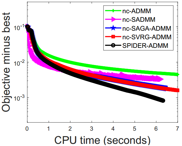
(a) a9a

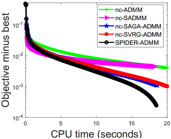
(b) w8a

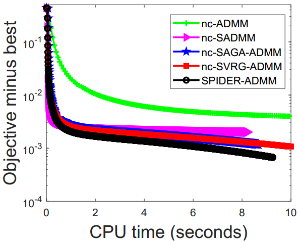
(c) ijcnn1

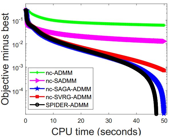
(d) covtype.binary

Figure 1: Objective value versus CPU time of the nonconvex graph-guided binary classification model on some real datasets.

6.1 Graph-Guided Binary Classification

In the subsection, we focus on the binary classification task. Specifically, given a set of training samples $(a_{i},b_{i})_{i=1}^{n}$, where $a_{i}\in\mathbb{R}^{d}$, $b_{i}\in\{-1,1\}$, then we solve the following nonconvex empirical loss minimization problem:

$$\min_{x\in\mathbb{R}^{d}}\ \frac{1}{n}\sum_{i=1}^{n}f_{i}(x)+\lambda\|Ax\|_{1},$$ (9)

where $f_{i}(x)=\frac{1}{1+\exp(b_{i}a_{i}^{T}x)}$ is the nonconvex sigmoid loss function. We use the nonsmooth regularizer i.e., graph-guided fused lasso (Kim et al., 2009), and $A$ decodes the sparsity pattern of graph, which is obtained by sparse precision matrix estimation (Friedman et al., 2008). To solve the problem (9), we give an auxiliary variable $y$ with the constraint $y=Ax$. In the experiment, we fix the parameter $\lambda=10^{-5}$, and use the same initial solution $x_{0}$ from the standard normal distribution for all algorithms.

Figure 1 shows that the objective values of our SPIDER-ADMM method faster decrease than those of other methods, as CPU time consumed increases. Thus, these results demonstrate that our method has a relatively faster convergence rate than other methods.

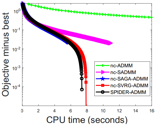
(a) letter

(b) sensorless

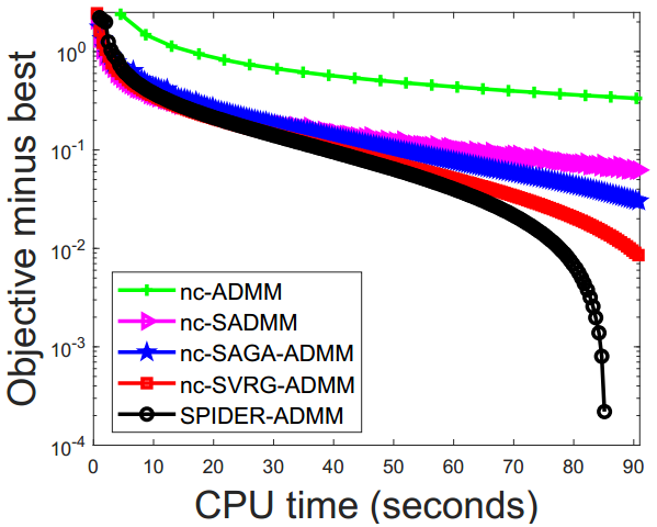
(c) mnist

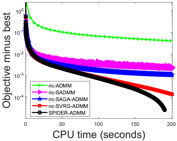
(d) covtype

Figure 2: Objective value versus CPU time of the nonconvex multi-task learning on some real datasets.

6.2 Multi-Task Learning

In this subsection, we focus on the multi-task learning task with sparse and low-rank structures. Specifically, given a set of training samples $(a_{i},b_{i})_{i=1}^{n}$, where $a_{i}\in\mathbb{R}^{d}$ and $b_{i}\in\{1,2,\cdots,c\}$, then let $D\in\mathbb{R}^{n\times c}$ with $D_{ij}=1$ if $j=b_{i}$, and $D_{ij}=0$ otherwise. This multi-task learning is equivalent to solving the following nonconvex problem:

$$\min_{X\in\mathbb{R}^{c\times d}}\ \frac{1}{n}\sum_{i=1}^{n}f_{i}(X)+\lambda_{1}\sum_{ij}\kappa(|X_{ij}|)+\lambda_{2}\|X\|_{*},$$ (10)

where $f_{i}(X)=\log(\sum_{j=1}^{c}\exp(X_{j,.}a_{i}))-\sum_{j=1}^{c}D_{ij}X_{j,.}a_{i}$ is a multinomial logistic loss function, $\kappa(|X_{ij}|)=\beta\log(1+\frac{|X_{ij}|}{\alpha})$ is the nonconvex log-sum penalty function (Candes et al., 2008). Next, we change the above problem into the following form:

$$\min \quad\frac{1}{n}\sum_{i=1}^{n}\bar{f}_{i}(X)+\lambda_{1}\kappa_{0}\|Y_{1}\|_{1}+\lambda_{2}\|Y_{2}\|_{*}$$ (11)

s.t. $$\quad AX+B_{1}Y_{1}+B_{2}Y_{2}=0,$$

where $\bar{f}_{i}(X)=f_{i}(X)+\lambda_{1}\big{(}\sum_{ij}\kappa(|X_{ij}|)-\kappa_{0}\|X\|_{1}\big{)}$, and $\kappa_{0}=\kappa^{\prime}(0)$. Here $A=[I_{c};I_{c}]\in\mathbb{R}^{2c\times c}$, $B_{1}=[-I_{c};0]\in\mathbb{R}^{2c\times c}$ and $B_{2}=[0;-I]$. By the Proposition 2.3 in Yao & Kwok (2016), $\bar{f}_{i}(X)$ is nonconvex and smooth. In the experiment, we fix the parameters $\lambda_{1}=10^{-5}$ and $\lambda_{2}=10^{-4}$, and use the same initial solution $x_{0}$ from the standard normal distribution for all algorithms.

Figure 2 shows that objective values of our SPIDER-ADMM faster decrease than those of the other methods, as CPU time consumed increases. Similarly, these results also demonstrate that our method has a relatively faster convergence rate than other methods.

7 Conclusion

In the paper, we proposed a faster stochastic ADMM method (i.e., SPIDER-ADMM) for nonconvex optimization. Moreover, we proved that the SPIDER-ADMM achieves a lower IFO complexity of $\mathcal{O}(n+n^{1/2}\epsilon^{-1})$. Further, we extended the SPIDER-ADMM to the online setting, and proposed a faster online ADMM method (i.e., online SPIDER-ADMM). As one of major contribution of this paper, we provided a new theoretical analysis framework for the nonconvex stochastic ADMM methods with providing an optimal IFO complexity. Based on our new theoretical analysis framework, we studied the unsolved optimal IFO complexity of the existing non-convex SVRG-ADMM and SAGA-ADMM methods, and also proved that they reach an IFO complexity of $\mathcal{O}(n+n^{2/3}\epsilon^{-1})$. In the future work, we can apply the stage-wise stochastic momentum technique (Chen et al., 2018) to accelerate our algorithms.

Appendix A Supplementary Materials

In this section, we at detail provide the proof of the above lemmas and theorems. Throughout the paper, let $n_{k}=[k/q]$ such that $(n_{k}-1)q\leq k\leq n_{k}q-1$. First, we introduce a useful lemma from Fang et al. (2018).

Lemma 5.

(Fang et al., 2018) Under Assumption 1, the SPIDER generates stochastic gradient $v_{k}$ satisfies for all $(n_{k}-1)q+1\leq k\leq n_{k}q-1$,

$$\mathbb{E}\|v_{k}-\nabla f(x_{k})\|^{2}\leq\frac{L^{2}}{|S_{2}|}\mathbb{E}\|x_{k}-x_{k-1}\|^{2}+\mathbb{E}\|v_{k-1}-\nabla f(x_{k-1})\|^{2}.$$ (12)

From Lemma 1, telescoping (12) over $k$ from $(n_{k}-1)q+1$ to $k$, we have

$$\mathbb{E}\|v_{k}-\nabla f(x_{k})\|^{2}\leq\sum_{i=(n_{k}-1)q}^{k-1}\frac{L^{2}}{|S_{2}|}\mathbb{E}\|x_{i+1}-x_{i}\|^{2}+\mathbb{E}\|v_{(n_{k}-1)q}-\nabla f(x_{(n_{k}-1)q})\|^{2}.$$ (13)

In Algorithm 3, due to $v_{(n_{k}-1)q}=\nabla f(x_{(n_{k}-1)q})$ and $|S_{2}|=b$, we have

$$\mathbb{E}\|v_{k}-\nabla f(x_{k})\|^{2}\leq\sum_{i=(n_{k}-1)q}^{k-1}\frac{L^{2}}{b}\mathbb{E}\|x_{i+1}-x_{i}\|^{2}.$$ (14)

In Algorithm 4, by Assumption 2 and $|S_{2}|=b_{2}$, we have

$$\mathbb{E}\|v_{k}-\nabla f(x_{k})\|^{2}\leq\sum_{i=(n_{k}-1)q}^{k-1}\frac{L^{2}}{b_{2}}\mathbb{E}\|x_{i+1}-x_{i}\|^{2}+\frac{\delta^{2}}{b_{1}}.$$ (15)

Notations: To make the paper easier to follow, we give the following notations:

• $\|\cdot\|$ denotes the vector $\ell_{2}$ norm and the matrix spectral norm, respectively.

• $\|x\|_{G}=\sqrt{x^{T}Gx}$, where $G$ is a positive definite matrix.

• $\sigma^{A}_{\min}$ and $\sigma^{A}_{\max}$ denotes the minimum and maximum eigenvalues of $A^{T}A$, respectively; the conditional number $\kappa_{A}=\frac{\sigma_{\max}^{A}}{\sigma_{\min}^{A}}$.

• $\sigma^{B_{j}}_{\max}$ denotes the maximum eigenvalues of $B_{j}^{T}B_{j}$ for all $j\in[k]$, and $\sigma^{B}_{\max}=\max_{j=1}^{k}\sigma^{B_{j}}_{\max}$.

• $\sigma_{\min}(G)$ and $\sigma_{\max}(G)$ denotes the minimum and maximum eigenvalues of matrix $G$, respectively; the conditional number $\kappa_{G}=\frac{\sigma_{\max}(G)}{\sigma_{\min}(G)}$.

• $\eta$ denotes the step size of updating variable $x$.

• $L$ denotes the Lipschitz constant of $\nabla f(x)$.

• $b$ denotes the mini-batch size of stochastic gradient.

• In both SPIDER-ADMM and online SPIDER-ADMM, $K$ denotes the total number of iteration. In both SVRG-ADMM and SAGA-ADMM, $T$, $M$ and $S$ are the total number of iterations, the number of iterations in the inner loop, and the number of iterations in the outer loop, respectively.

• In SVRG-ADMM algorithm, $y_{j}^{s,t}$ denotes output of the variable $y_{j}$ in $t$-th inner loop and $s$-th outer loop.

A.1 Convergence Analysis of the SPIDER-ADMM

In this subsection, we conduct convergence analysis of the SPIDER-ADMM. We begin with giving some useful lemmas.

Lemma 6.

Under Assumption 1 and given the sequence $\{x_{k},y_{[m]}^{k},z_{k}\}_{k=1}^{K}$ from Algorithm 3, it holds that

$$\mathbb{E}\|z_{k+1}-z_{k}\|^{2}\leq \frac{18L^{2}}{\sigma^{A}_{\min}b}\sum_{i=(n_{k}-1)q}^{k-1}\mathbb{E}\|x_{i+1}-x_{i}\|^{2}+(\frac{9L^{2}}{\sigma^{A}_{\min}}+\frac{3\sigma^{2}_{\max}(G)}{\sigma^{A}_{\min}\eta^{2}})\|x_{k}-x_{k-1}\|^{2}$$

$$+\frac{3\sigma^{2}_{\max}(G)}{\sigma^{A}_{\min}\eta^{2}}\|x_{k+1}-x_{k}\|^{2}.$$ (16)

Proof.

Using the optimal condition of the step 10 in Algorithm 3, we have

$$v_{k}+\frac{G}{\eta}(x_{k+1}-x_{k})-A^{T}z_{k}+\rho A^{T}(Ax_{k+1}+\sum_{j=1}^{m}B_{j}y_{j}^{k+1}-c)=0.$$ (17)

Then using the step 11 of Algorithm 3, we have

$$A^{T}z_{k+1}=v_{k}+\frac{G}{\eta}(x_{k+1}-x_{k}).$$ (18)

It follows that

$$A^{T}(z_{k+1}-z_{k})= v_{k}-v_{k-1}+\frac{G}{\eta}(x_{k+1}-x_{k})-\frac{G}{\eta}(x_{k}-x_{k-1}).$$ (19)

By (19), we have

$$\mathbb{E}\|z_{k+1}-z_{k}\|^{2}\leq\frac{1}{\sigma^{A}_{\min}}\big{[}3\mathbb{E}\|v_{k}-v_{k-1}\|^{2}+\frac{3\sigma^{2}_{\max}(G)}{\eta^{2}}\mathbb{E}\|x_{k+1}-x_{k}\|^{2}+\frac{3\sigma^{2}_{\max}(G)}{\eta^{2}}\mathbb{E}\|x_{k}-x_{k-1}\|^{2}\big{]},$$ (20)

where the inequality holds by the Jensen’s inequality yielding $\|\frac{1}{n}\sum_{i=1}^{n}z_{i}\|^{2}\leq\frac{1}{n}\sum_{i=1}^{n}\|z_{i}\|^{2}$.

Next, considering the upper bound of $\|v_{k}-v_{k-1}\|^{2}$, we have

$$\mathbb{E}\|v_{k}-v_{k-1}\|^{2} =\mathbb{E}\|v_{k}-\nabla f(x_{k})+\nabla f(x_{k})-\nabla f(x_{k-1})+\nabla f(x_{k-1})-v_{k-1}\|^{2}$$

$$\leq 3\mathbb{E}\|v_{k}-\nabla f(x_{k})\|^{2}+3\mathbb{E}\|\nabla f(x_{k})-\nabla f(x_{k-1})\|^{2}+3\mathbb{E}\|\nabla f(x_{k-1})-v_{k-1}\|^{2}$$

$$\leq\frac{3L^{2}}{b}\sum_{i=(n_{k}-1)q}^{k-1}\mathbb{E}\|x_{i+1}-x_{i}\|^{2}+3L^{2}\mathbb{E}\|x_{k-1}-x_{k}\|^{2}+\frac{3L^{2}}{b}\sum_{i=(n_{k}-1)q}^{k-2}\mathbb{E}\|x_{i+1}-x_{i}\|^{2}$$

$$\leq\frac{6L^{2}}{b}\sum_{i=(n_{k}-1)q}^{k-1}\mathbb{E}\|x_{i+1}-x_{i}\|^{2}+3L^{2}\mathbb{E}\|x_{k-1}-x_{k}\|^{2},$$ (21)

where the second inequality holds by Assumption 1 and the inequality (14).

Finally, combining the inequalities (20) and (A.1), we obtain the above result.

∎

Lemma 7.

Suppose the sequence $\{x_{k},y_{[m]}^{k},z_{k}\}_{k=1}^{K}$ is generated from Algorithm 3, and define a Lyapunov function $R_{k}$ as follows:

$$R_{k}=\mathcal{L}_{\rho}(x_{k},y_{[m]}^{k},z_{k})+(\frac{9L^{2}}{\sigma^{A}_{\min}\rho}+\frac{3\kappa_{A}\sigma^{2}_{\max}(G)}{\sigma^{A}_{\min}\eta^{2}\rho})\|x_{k}-x_{k-1}\|^{2}+\frac{2\kappa_{A}L^{2}}{\sigma^{A}_{\min}\rho b}\sum_{i=(n_{k}-1)q}^{k-1}\mathbb{E}\|x_{i+1}-x_{i}\|^{2}.$$ (22)

Let $b=q$, $\eta=\frac{2\alpha\sigma_{\min}(G)}{3L}\ (0<\alpha\leq 1)$ and $\rho=\frac{\sqrt{170\kappa_{A}}\kappa_{G}L}{\sigma^{A}_{\min}\alpha}$, then we have

$$\frac{1}{K}\sum_{i=0}^{K-1}(\|x_{i+1}-x_{i}\|^{2}+\sum_{j=1}^{m}\|y_{j}^{i}-y_{j}^{i+1}\|^{2})\leq\frac{\mathbb{E}[R_{0}]-R^{*}}{K\gamma},$$ (23)

where $\gamma=\min(\chi,\sigma_{\min}^{H})$ with $\chi\geq\frac{\sqrt{170\kappa_{A}}\kappa_{G}L}{4\alpha}$ and $R^{*}$ is a lower bound of the function $R_{k}$.

Proof.

By the optimal condition of step 9 in Algorithm 3, we have, for $j\in[m]$

$$0 =(y_{j}^{k}-y_{j}^{k+1})^{T}\big{(}\partial g_{j}(y_{j}^{k+1})-B^{T}z_{k}+\rho B^{T}(Ax_{k}+\sum_{i=1}^{j}B_{i}y_{i}^{k+1}+\sum_{i=j+1}^{m}B_{i}y_{i}^{k}-c)+H_{j}(y_{j}^{k+1}-y_{j}^{k})\big{)}$$

$$\leq g_{j}(y_{j}^{k})-g_{j}(y_{j}^{k+1})-(z_{k})^{T}(B_{j}y_{j}^{k}-B_{j}y_{j}^{k+1})+\rho(By_{j}^{k}-By_{j}^{k+1})^{T}(Ax_{k}+\sum_{i=1}^{j}B_{i}y_{i}^{k+1}+\sum_{i=j+1}^{m}B_{i}y_{i}^{k}-c)-\|y_{j}^{k+1}-y_{j}^{k}\|^{2}_{H_{j}}$$

$$=g_{j}(y_{j}^{k})-g_{j}(y_{j}^{k+1})-(z_{k})^{T}(Ax_{k}+\sum_{i=1}^{j-1}B_{i}y_{i}^{k+1}+\sum_{i=j}^{m}B_{i}y_{i}^{k}-c)+(z_{k})^{T}(Ax_{k}+\sum_{i=1}^{j}B_{i}y_{i}^{k+1}+\sum_{i=j+1}^{m}B_{i}y_{i}^{k}-c)$$

$$\quad+\frac{\rho}{2}\|Ax_{k}+\sum_{i=1}^{j-1}B_{i}y_{i}^{k+1}+\sum_{i=j}^{m}B_{i}y_{i}^{k}-c\|^{2}-\frac{\rho}{2}\|Ax_{k}+\sum_{i=1}^{j}B_{i}y_{i}^{k+1}+\sum_{i=j+1}^{m}B_{i}y_{i}^{k}-c\|^{2}-\frac{\rho}{2}\|B_{j}y_{j}^{k}-B_{j}y_{j}^{k+1}\|^{2}$$

$$\quad-\|y_{j}^{k+1}-y_{j}^{k}\|^{2}_{H_{j}}$$

$$\leq\underbrace{f(x_{k})+g_{j}(y_{j}^{k})-(z_{k})^{T}(Ax_{k}+\sum_{i=1}^{j-1}B_{i}y_{i}^{k+1}+\sum_{i=j}^{m}B_{i}y_{i}^{k}-c)+\frac{\rho}{2}\|Ax_{k}+\sum_{i=1}^{j-1}B_{i}y_{i}^{k+1}+\sum_{i=j}^{m}B_{i}y_{i}^{k}-c\|^{2}}_{\mathcal{L}_{\rho}(x_{k},y_{[j-1]}^{k+1},y_{[j:m]}^{k},z_{k})}-\|y_{j}^{k+1}-y_{j}^{k}\|^{2}_{H_{j}}$$

$$\quad-\underbrace{(f(x_{k})+g_{j}(y_{j}^{k+1})-(z_{k})^{T}(Ax_{k}+\sum_{i=1}^{j}B_{i}y_{i}^{k+1}+\sum_{i=j+1}^{m}B_{i}y_{i}^{k}-c)+\frac{\rho}{2}\|Ax_{k}+\sum_{i=1}^{j}B_{i}y_{i}^{k+1}+\sum_{i=j+1}^{m}B_{i}y_{i}^{k}-c\|^{2}}_{\mathcal{L}_{\rho}(x_{k},y_{[j]}^{k+1},y_{[j+1:m]}^{k},z_{k})}$$

$$\leq\mathcal{L}_{\rho}(x_{k},y_{[j-1]}^{k+1},y_{[j:m]}^{k},z_{k})-\mathcal{L}_{\rho}(x_{k},y_{[j]}^{k+1},y_{[j+1:m]}^{k},z_{k})-\sigma_{\min}(H_{j})\|y_{j}^{k}-y_{j}^{k+1}\|^{2},$$ (24)

where the first inequality holds by the convexity of function $g_{j}(y)$, and the second equality follows by applying the equality $(a-b)^{T}b=\frac{1}{2}(\|a\|^{2}-\|b\|^{2}-\|a-b\|^{2})$ on the term $(By_{j}^{k}-By_{j}^{k+1})^{T}(Ax_{k}+\sum_{i=1}^{j}B_{i}y_{i}^{k+1}+\sum_{i=j+1}^{m}B_{i}y_{i}^{k}-c)$. Thus, we have, for all $j\in[m]$

$$\mathcal{L}_{\rho}(x_{k},y_{[j-1]}^{k+1},y_{[j:m]}^{k},z_{k})\leq\mathcal{L}_{\rho}(x_{k},y_{[j]}^{k+1},y_{[j+1:m]}^{k},z_{k})-\sigma_{\min}(H_{j})\|y_{j}^{k}-y_{j}^{k+1}\|^{2}.$$ (25)

Telescoping inequality (25) over $j$ from $1$ to $m$, we obtain

$$\mathcal{L}_{\rho}(x_{k},y^{k+1}_{[m]},z_{k})\leq\mathcal{L}_{\rho}(x_{k},y^{k}_{[m]},z_{k})-\sigma_{\min}^{H}\sum_{j=1}^{m}\|y_{j}^{k}-y_{j}^{k+1}\|^{2}.$$ (26)

where $\sigma_{\min}^{H}=\min_{j\in[m]}\sigma_{\min}(H_{j})$.

By Assumption 1, we have

$$0\leq f(x_{k})-f(x_{k+1})+\nabla f(x_{k})^{T}(x_{k+1}-x_{k})+\frac{L}{2}\|x_{k+1}-x_{k}\|^{2}.$$ (27)

Using the optimal condition of step 10 in Algorithm 3, we have

$$0=(x_{k}-x_{k+1})^{T}\big{(}v_{k}-A^{T}z_{k}+\rho A^{T}(Ax_{k+1}+\sum_{j=1}^{m}B_{j}y_{j}^{k+1}-c)+\frac{G}{\eta}(x_{k+1}-x_{k})\big{)}.$$ (28)

Combining (27) and (28), we have

$$0 \leq f(x_{k})-f(x_{k+1})+\nabla f(x_{k})^{T}(x_{k+1}-x_{k})+\frac{L}{2}\|x_{k+1}-x_{k}\|^{2}$$

$$\quad+(x_{k}-x_{k+1})^{T}\big{(}v_{k}-A^{T}z_{k}+\rho A^{T}(Ax_{k+1}+\sum_{j=1}^{m}B_{j}y_{j}^{k+1}-c)+\frac{G}{\eta}(x_{k+1}-x_{k})\big{)}$$

$$=f(x_{k})-f(x_{k+1})+\frac{L}{2}\|x_{k}-x_{k+1}\|^{2}-\frac{1}{\eta}\|x_{k}-x_{k+1}\|^{2}_{G}+(x_{k}-x_{k+1})^{T}(v_{k}-\nabla f(x_{k}))$$

$$\quad-(z_{k})^{T}(Ax_{k}-Ax_{k+1})+\rho(Ax_{k}-Ax_{k+1})^{T}(Ax_{k+1}+\sum_{j=1}^{m}B_{j}y_{j}^{k+1}-c)$$

$$=f(x_{k})-f(x_{k+1})+\frac{L}{2}\|x_{k}-x_{k+1}\|^{2}-\frac{1}{\eta}\|x_{k}-x_{k+1}\|^{2}_{G}+(x_{k}-x_{k+1})^{T}\big{(}v_{k}-\nabla f(x_{k})\big{)}-(z_{k})^{T}(Ax_{k}+\sum_{j=1}^{m}B_{j}y_{j}^{k+1}-c)$$

$$\quad+(z_{k})^{T}(Ax_{k+1}+\sum_{j=1}^{m}B_{j}y_{j}^{k+1}-c)+\frac{\rho}{2}\big{(}\|Ax_{k}+\sum_{j=1}^{m}B_{j}y_{j}^{k+1}-c\|^{2}-\|Ax_{k+1}+\sum_{j=1}^{m}B_{j}y_{j}^{k+1}-c\|^{2}-\|Ax_{k}-Ax_{k+1}\|^{2}\big{)}$$

$$=\underbrace{f(x_{k})-z_{k}^{T}(Ax_{k}+\sum_{j=1}^{m}B_{j}y_{j}^{k+1}-c)+\frac{\rho}{2}\|Ax_{k}+\sum_{j=1}^{m}B_{j}y_{j}^{k+1}-c\|^{2}}_{L_{\rho}(x_{k},y_{[m]}^{k+1},z_{k})}+\frac{L}{2}\|x_{k}-x_{k+1}\|^{2}+(x_{k}-x_{k+1})^{T}\big{(}v_{k}-\nabla f(x_{k})\big{)}$$

$$\quad-\underbrace{\big{(}f(x_{k+1})-z_{k}^{T}(Ax_{k+1}+\sum_{j=1}^{m}B_{j}y_{j}^{k+1}-c)+\frac{\rho}{2}\|Ax_{k+1}+\sum_{j=1}^{m}B_{j}y_{j}^{k+1}-c\|^{2}\big{)}}_{L_{\rho}(x_{k+1},y^{k+1}_{[m]},z_{k})}-\frac{1}{\eta}\|x_{k}-x_{k+1}\|^{2}_{G}-\frac{\rho}{2}\|Ax_{k}-Ax_{k+1}\|^{2}$$

$$\leq\mathcal{L}_{\rho}(x_{k},y_{[m]}^{k+1},z_{k})-\mathcal{L}_{\rho}(x_{k+1},y_{[m]}^{k+1},z_{k})-(\frac{\sigma_{\min}(G)}{\eta}+\frac{\rho\sigma^{A}_{\min}}{2}-\frac{L}{2})\|x_{k+1}-x_{k}\|^{2}+(x_{k}-x_{k+1})^{T}(v_{k}-\nabla f(x_{k}))$$

$$\leq\mathcal{L}_{\rho}(x_{k},y_{[m]}^{k+1},z_{k})-\mathcal{L}_{\rho}(x_{k+1},y_{[m]}^{k+1},z_{k})-(\frac{\sigma_{\min}(G)}{\eta}+\frac{\rho\sigma^{A}_{\min}}{2}-L)\|x_{k+1}-x_{k}\|^{2}+\frac{1}{2L}\|v_{k}-\nabla f(x_{k})\|^{2}$$

$$\leq\mathcal{L}_{\rho}(x_{k},y_{[m]}^{k+1},z_{k})-\mathcal{L}_{\rho}(x_{k+1},y_{[m]}^{k+1},z_{k})-(\frac{\sigma_{\min}(G)}{\eta}+\frac{\rho\sigma^{A}_{\min}}{2}-L)\|x_{k+1}-x_{k}\|^{2}+\frac{L}{2b}\sum_{i=(n_{k}-1)q}^{k-1}\mathbb{E}\|x_{i+1}-x_{i}\|^{2},$$

where the second equality follows by applying the equality $(a-b)^{T}b=\frac{1}{2}(\|a\|^{2}-\|b\|^{2}-\|a-b\|^{2})$ over the term $(Ax_{k}-Ax_{k+1})^{T}(Ax_{k+1}+\sum_{j=1}^{m}B_{j}y_{j}^{k+1}-c)$; the third inequality follows by the inequality $a^{T}b\leq\frac{1}{2L}\|a\|^{2}+\frac{L}{2}\|b\|^{2}$, and the forth inequality holds by the inequality (14). It follows that

$$\mathcal{L}_{\rho}(x_{k+1},y_{[m]}^{k+1},z_{k})\leq\mathcal{L}_{\rho}(x_{k},y_{[m]}^{k+1},z_{k})-(\frac{\sigma_{\min}(G)}{\eta}+\frac{\rho\sigma^{A}_{\min}}{2}-L)\|x_{k+1}-x_{k}\|^{2}+\frac{L}{2b}\sum_{i=(n_{k}-1)q}^{k-1}\mathbb{E}\|x_{i+1}-x_{i}\|^{2}.$$ (29)

Using the step 10 in Algorithm 3, we have

$$\mathcal{L}_{\rho}(x_{k+1},y_{[m]}^{k+1},z_{k+1})-\mathcal{L}_{\rho}(x_{k+1},y_{[m]}^{k+1},z_{k}) =\frac{1}{\rho}\|z_{k+1}-z_{k}\|^{2}$$

$$\leq\frac{18L^{2}}{\sigma^{A}_{\min}b\rho}\sum_{i=(n_{k}-1)q}^{k-1}\mathbb{E}\|x_{i+1}-x_{i}\|^{2}+(\frac{9L^{2}}{\sigma^{A}_{\min}\rho}+\frac{3\sigma^{2}_{\max}(G)}{\sigma^{A}_{\min}\eta^{2}\rho})\|x_{k}-x_{k-1}\|^{2}$$

$$+\frac{3\sigma^{2}_{\max}(G)}{\sigma^{A}_{\min}\eta^{2}\rho}\|x_{k+1}-x_{k}\|^{2},$$ (30)

where the above inequality holds by Lemma 6.

Combining (26), (29) and (A.1), we have

$$\mathcal{L}_{\rho}(x_{k+1},y_{[m]}^{k+1},z_{k+1}) \leq\mathcal{L}_{\rho}(x_{k},y_{[m]}^{k},z_{k})-\sigma_{\min}^{H}\sum_{j=1}^{m}\|y_{j}^{k}-y_{j}^{k+1}\|^{2}-(\frac{\sigma_{\min}(G)}{\eta}+\frac{\rho\sigma^{A}_{\min}}{2}-L-\frac{3\sigma^{2}_{\max}(G)}{\sigma^{A}_{\min}\eta^{2}\rho})\|x_{k+1}-x_{k}\|^{2}$$

$$\quad+(\frac{L}{2b}+\frac{18L^{2}}{\sigma^{A}_{\min}b\rho})\sum_{i=(n_{k}-1)q}^{k-1}\mathbb{E}\|x_{i+1}-x_{i}\|^{2}+(\frac{9L^{2}}{\sigma^{A}_{\min}\rho}+\frac{3\sigma^{2}_{\max}(G)}{\sigma^{A}_{\min}\eta^{2}\rho})\|x_{k}-x_{k-1}\|^{2}.$$ (31)

Next, we define a Lyapunov function $R_{k}$:

$$R_{k}=\mathcal{L}_{\rho}(x_{k},y_{[m]}^{k},z_{k})+(\frac{9L^{2}}{\sigma^{A}_{\min}\rho}+\frac{3\kappa_{A}\sigma^{2}_{\max}(G)}{\sigma^{A}_{\min}\eta^{2}\rho})\|x_{k}-x_{k-1}\|^{2}+\frac{2\kappa_{A}L^{2}}{\sigma^{A}_{\min}\rho b}\sum_{i=(n_{k}-1)q}^{k-1}\mathbb{E}\|x_{i+1}-x_{i}\|^{2}.$$ (32)

Since

$$\sum_{i=(n_{k}-1)q}^{k}\mathbb{E}\|x_{i+1}-x_{i}\|^{2}=\sum_{i=(n_{k}-1)q}^{k-1}\mathbb{E}\|x_{i+1}-x_{i}\|^{2}+\|x_{k+1}-x_{k}\|^{2},$$

and $\kappa_{A}\geq 1$, the inequality (A.1) can be rewrite as follows:

$$R_{k+1} \leq R_{k}-(\frac{\sigma_{\min}(G)}{\eta}+\frac{\rho\sigma^{A}_{\min}}{2}-L-\frac{6\kappa_{A}\sigma^{2}_{\max}(G)}{\sigma^{A}_{\min}\eta^{2}\rho}-\frac{9L^{2}}{\sigma^{A}_{\min}\rho}-\frac{2\kappa_{A}L^{2}}{\sigma^{A}_{\min}\rho b})\|x_{k+1}-x_{k}\|^{2}$$

$$\quad-\sigma_{\min}^{H}\sum_{j=1}^{m}\|y_{j}^{k}-y_{j}^{k+1}\|^{2}+(\frac{L}{2b}+\frac{18L^{2}}{\sigma^{A}_{\min}b\rho})\sum_{i=(n_{k}-1)q}^{k-1}\mathbb{E}\|x_{i+1}-x_{i}\|^{2}.$$ (33)

Then telescoping equality (A.1) over $k$ from $(n_{k}-1)q$ to $k$ where $k\leq n_{k}q-1$ and let $n_{j}=n_{k}$ for $(n_{k}-1)q\leq j\leq n_{k}q-1$, we have

$$\mathbb{E}[R_{k+1}] \leq\mathbb{E}[R_{(n_{k}-1)q}]-(\frac{\sigma_{\min}(G)}{\eta}+\frac{\rho\sigma^{A}_{\min}}{2}-L-\frac{6\kappa_{A}\sigma^{2}_{\max}(G)}{\sigma^{A}_{\min}\eta^{2}\rho}-\frac{9L^{2}}{\sigma^{A}_{\min}\rho}-\frac{2\kappa_{A}L^{2}}{\sigma^{A}_{\min}\rho b})\sum_{j=(n_{k}-1)q}^{k}\|x_{j+1}-x_{j}\|^{2}$$

$$-\sigma_{\min}^{H}\sum_{i=(n_{k}-1)q}^{k}\sum_{j=1}^{m}\|y_{j}^{i}-y_{j}^{i+1}\|^{2}+(\frac{L}{2b}+\frac{18L^{2}}{\sigma^{A}_{\min}b\rho})\sum_{j=(n_{k}-1)q}^{k}\sum_{i=(n_{k}-1)q}^{k-1}\mathbb{E}\|x_{i+1}-x_{i}\|^{2}$$

$$\leq\mathbb{E}[R_{(n_{k}-1)q}]-(\frac{\sigma_{\min}(G)}{\eta}+\frac{\rho\sigma^{A}_{\min}}{2}-L-\frac{6\kappa_{A}\sigma^{2}_{\max}(G)}{\sigma^{A}_{\min}\eta^{2}\rho}-\frac{9L^{2}}{\sigma^{A}_{\min}\rho}-\frac{2\kappa_{A}L^{2}}{\sigma^{A}_{\min}\rho b})\sum_{i=(n_{k}-1)q}^{k}\|x_{i+1}-x_{i}\|^{2}$$

$$-\sigma_{\min}^{H}\sum_{i=(n_{k}-1)q}^{k-1}\sum_{j=1}^{m}\|y_{j}^{i}-y_{j}^{i+1}\|^{2}+(\frac{Lq}{2b}+\frac{18L^{2}q}{\sigma^{A}_{\min}b\rho})\sum_{i=(n_{k}-1)q}^{k}\mathbb{E}\|x_{i+1}-x_{i}\|^{2}$$

$$=\mathbb{E}[R_{(n_{k}-1)q}]-(\frac{\sigma_{\min}(G)}{\eta}+\frac{\rho\sigma^{A}_{\min}}{2}-L-\frac{6\kappa_{A}\sigma^{2}_{\max}(G)}{\sigma^{A}_{\min}\eta^{2}\rho}-\frac{9L^{2}}{\sigma^{A}_{\min}\rho}-\frac{2\kappa_{A}L^{2}}{\sigma^{A}_{\min}\rho b}-\frac{Lq}{2b}-\frac{18L^{2}q}{\sigma^{A}_{\min}b\rho})\sum_{i=(n_{k}-1)q}^{k}\|x_{i+1}-x_{i}\|^{2}$$

$$\quad-\sigma_{\min}^{H}\sum_{i=(n_{k}-1)q}^{k-1}\sum_{j=1}^{m}\|y_{j}^{i}-y_{j}^{i+1}\|^{2},$$ (34)

where the second inequality holds by the fact that

$$\sum_{j=(n_{k}-1)q}^{k}\sum_{i=(n_{k}-1)q}^{k-1}\mathbb{E}\|x_{i+1}-x_{i}\|^{2}\leq\sum_{j=(n_{k}-1)q}^{k}\sum_{i=(n_{k}-1)q}^{k}\mathbb{E}\|x_{i+1}-x_{i}\|^{2}\leq q\sum_{i=(n_{k}-1)q}^{k}\mathbb{E}\|x_{i+1}-x_{i}\|^{2}.$$

Since $b=q$, we have

$$\chi =\frac{\sigma_{\min}(G)}{\eta}+\frac{\rho\sigma^{A}_{\min}}{2}-L-\frac{6\sigma^{2}_{\max}(G)}{\sigma^{A}_{\min}\eta^{2}\rho}-\frac{9L^{2}}{\sigma^{A}_{\min}\rho}-\frac{2\kappa_{A}L^{2}}{\sigma^{A}_{\min}\rho b}-\frac{Lq}{2b}-\frac{18L^{2}q}{\sigma^{A}_{\min}b\rho}$$

$$=\underbrace{\frac{\sigma_{\min}(G)}{\eta}-\frac{3L}{2}}_{L_{1}}+\underbrace{\frac{\rho\sigma^{A}_{\min}}{2}-\frac{6\sigma^{2}_{\max}(G)}{\sigma^{A}_{\min}\eta^{2}\rho}-\frac{27L^{2}}{\sigma^{A}_{\min}\rho}-\frac{2\kappa_{A}L^{2}}{\sigma^{A}_{\min}\rho b}}_{L_{2}}.$$ (35)

Given $0<\eta\leq\frac{2\sigma_{\min}(G)}{3L}$, we have $L_{1}\geq 0$. Further, let $\eta=\frac{2\alpha\sigma_{\min}(G)}{3L}\ (0<\alpha\leq 1)$ and $\rho=\frac{\sqrt{170\kappa_{A}}\kappa_{G}L}{\sigma^{A}_{\min}\alpha}$, we have

$$L_{2} =\frac{\rho\sigma^{A}_{\min}}{2}-\frac{6\sigma^{2}_{\max}(G)}{\sigma^{A}_{\min}\eta^{2}\rho}-\frac{27L^{2}}{\sigma^{A}_{\min}\rho}-\frac{2\kappa_{A}L^{2}}{\sigma^{A}_{\min}\rho b}$$

$$=\frac{\rho\sigma^{A}_{\min}}{2}-\frac{27L^{2}\kappa^{2}_{G}}{2\sigma^{A}_{\min}\rho\alpha^{2}}-\frac{27L^{2}}{\sigma^{A}_{\min}\rho}-\frac{2\kappa_{A}L^{2}}{\sigma^{A}_{\min}\rho b}$$

$$\geq\frac{\rho\sigma^{A}_{\min}}{2}-\frac{27L^{2}\kappa^{2}_{G}\kappa_{A}}{2\sigma^{A}_{\min}\rho\alpha^{2}}-\frac{27L^{2}\kappa^{2}_{G}\kappa_{A}}{\sigma^{A}_{\min}\rho\alpha^{2}}-\frac{2\kappa^{2}_{G}\kappa_{A}L^{2}}{\sigma^{A}_{\min}\rho\alpha^{2}}$$

$$\geq\frac{\rho\sigma^{A}_{\min}}{4}+\underbrace{\frac{\rho\sigma^{A}_{\min}}{4}-\frac{85L^{2}\kappa^{2}_{G}\kappa_{A}}{2\sigma^{A}_{\min}\rho\alpha^{2}}}_{\geq 0}$$

$$\geq\frac{\sqrt{170\kappa_{A}}\kappa_{G}L}{4\alpha},$$ (36)

where the first inequality holds by $\kappa_{G}=\geq 1$ and $b\geq 1\geq\alpha^{2}$ and the third equality holds by $\rho=\frac{\sqrt{170\kappa_{A}}\kappa_{G}L}{\sigma^{A}_{\min}\alpha}$. Thus, we obtain $\chi\geq\frac{\sqrt{170\kappa_{A}}\kappa_{G}L}{4\alpha}$.

Next, using (18), we have

$$z_{k+1}=(A^{T})^{+}(v_{k}+\frac{G}{\eta}(x_{k+1}-x_{k})),$$ (37)

where $(A^{T})^{+}$ is the pseudoinverse of $A^{T}$. Due to that $A$ is full row rank, we have $(A^{T})^{+}=(AA^{T})^{-1}A$. It follows that $\sigma_{\max}((A^{T})^{+})^{T}(A^{T})^{+})\leq\frac{\sigma_{\max}^{A}}{(\sigma^{A}_{\min})^{2}}=\frac{\kappa_{A}}{\sigma^{A}_{\min}}$.

Then we have

$$\mathcal{L}_{\rho}(x_{k+1},y_{[m]}^{k+1},z_{k+1})=f(x_{k+1})+\sum_{j=1}^{m}g_{j}(y_{j}^{k+1})-z_{k+1}^{T}(Ax_{k+1}+\sum_{j=1}^{m}B_{j}y_{j}^{k+1}-c)+\frac{\rho}{2}\|Ax_{k+1}+\sum_{j=1}^{m}B_{j}y_{j}^{k+1}-c\|^{2}$$

$$=f(x_{k+1})+\sum_{j=1}^{m}g_{j}(y_{j}^{k+1})-\langle(A^{T})^{+}(v_{k}+\frac{G}{\eta}(x_{k+1}-x_{k})),Ax_{k+1}+\sum_{j=1}^{m}B_{j}y_{j}^{k+1}-c\rangle+\frac{\rho}{2}\|Ax_{k+1}+\sum_{j=1}^{m}B_{j}y_{j}^{k+1}-c\|^{2}$$

$$=f(x_{k+1})+\sum_{j=1}^{m}g_{j}(y_{j}^{k+1})-\langle(A^{T})^{+}(v_{k}-\nabla f(x_{k})+\nabla f(x_{k})+\frac{G}{\eta}(x_{k+1}-x_{k})),Ax_{k+1}+\sum_{j=1}^{m}B_{j}y_{j}^{k+1}-c\rangle$$

$$\quad+\frac{\rho}{2}\|Ax_{k+1}+\sum_{j=1}^{m}B_{j}y_{j}^{k+1}-c\|^{2}$$

$$\geq f(x_{k+1})+\sum_{j=1}^{m}g_{j}(y_{j}^{k+1})-\frac{2\kappa_{A}}{\sigma^{A}_{\min}\rho}\|v_{k}-\nabla f(x_{k})\|^{2}-\frac{2\kappa_{A}}{\sigma^{A}_{\min}\rho}\|\nabla f(x_{k})\|^{2}-\frac{2\kappa_{A}\sigma^{2}_{\max}(G)}{\sigma^{A}_{\min}\eta^{2}\rho}\|x_{k+1}-x_{k}\|^{2}$$

$$\quad+\frac{\rho}{8}\|Ax_{k+1}+\sum_{j=1}^{m}B_{j}y_{j}^{k+1}-c\|^{2}$$

$$\geq f(x_{k+1})+\sum_{j=1}^{m}g_{j}(y_{j}^{k+1})-\frac{2\kappa_{A}L^{2}}{\sigma^{A}_{\min}b\rho}\sum_{i=(n_{k}-1)q}^{k-1}\mathbb{E}\|x_{i+1}-x_{i}\|^{2}-\frac{2\kappa_{A}\delta^{2}}{\sigma^{A}_{\min}\rho}-\frac{2\kappa_{A}\sigma^{2}_{\max}(G)}{\sigma^{A}_{\min}\eta^{2}\rho}\|x_{k+1}-x_{k}\|^{2}$$ (38)

where the first inequality is obtained by applying $\langle a,b\rangle\leq\frac{1}{2\beta}\|a\|^{2}+\frac{\beta}{2}\|b\|^{2}$ to the terms $\langle(A^{T})^{+}(v_{k}-\nabla f(x_{k})),Ax_{k+1}+By_{[m]}^{k+1}-c\rangle$, $\langle(A^{T})^{+}v_{k},Ax_{k+1}+By_{[m]}^{k+1}-c\rangle$ and $\langle(A^{T})^{+}\frac{G}{\eta}(x_{k+1}-x_{k}),Ax_{k+1}+By_{[m]}^{k+1}-c\rangle$ with $\beta=\frac{\rho}{4}$, respectively. The second inequality follows by the inequality (14) and Assumption 3. Therefore, we have, for $k=0,1,2,\cdots$

$$R_{k+1}\geq f^{*}+\sum_{j=1}^{m}g_{j}^{*}-\frac{2\kappa_{A}\delta^{2}}{\sigma^{A}_{\min}\rho}.$$ (39)

It follows that the function $R_{k}$ is bounded from below. Let $R^{*}$ denotes a low bound of function $R_{k}$.

Further, telescoping equality (A.1) over $k$ from $0$ to $K$, we have

$$\mathbb{E}[R_{K}]-\mathbb{E}[R_{0}] =(\mathbb{E}[R_{q}]-\mathbb{E}[R_{0}])+(\mathbb{E}[R_{2q}]-\mathbb{E}[R_{q}])+\cdots+(\mathbb{E}[R_{K}]-\mathbb{E}[R_{(n_{k}-1)q}])$$

$$\leq-\sum_{i=0}^{q-1}(\chi\|x_{i+1}-x_{i}\|^{2}+\sigma_{\min}^{H}\sum_{j=1}^{m}\|y_{j}^{k}-y_{j}^{k+1}\|^{2})-\sum_{i=q}^{2q-1}(\chi\|x_{i+1}-x_{i}\|^{2}+\sigma_{\min}^{H}\sum_{j=1}^{m}\|y_{j}^{k}-y_{j}^{k+1}\|^{2})$$

$$\quad-\cdots-\sum_{i=(n_{k}-1)q}^{K-1}(\chi\|x_{i+1}-x_{i}\|^{2}+\sigma_{\min}^{H}\sum_{j=1}^{m}\|y_{j}^{k}-y_{j}^{k+1}\|^{2})$$

$$=-\sum_{i=0}^{K-1}(\chi\|x_{i+1}-x_{i}\|^{2}+\sigma_{\min}^{H}\sum_{j=1}^{m}\|y_{j}^{k}-y_{j}^{k+1}\|^{2}).$$ (40)

Finally, we obtain

$$\frac{1}{K}\sum_{i=0}^{K-1}(\|x_{i+1}-x_{i}\|^{2}+\sum_{j=1}^{m}\|y_{j}^{i}-y_{j}^{i+1}\|^{2})\leq\frac{\mathbb{E}[R_{0}]-R^{*}}{K\gamma},$$ (41)

where $\gamma=\min(\chi,\sigma_{\min}^{H})$ with $\chi\geq\frac{\sqrt{170\kappa_{A}}\kappa_{G}L}{4\alpha}$.

∎

Theorem 5.

Suppose the sequence $\{x_{k},y_{[m]}^{k},z_{k})_{k=1}^{K}$ is generated from Algorithm 3, and let $b=q$, $\eta=\frac{2\alpha\sigma_{\min}(G)}{3L}\ (0<\alpha\leq 1)$, $\rho=\frac{\sqrt{170\kappa_{A}}\kappa_{G}L}{\sigma^{A}_{\min}\alpha}$, and

$$\nu_{1}=m\big{(}\rho^{2}\sigma^{B}_{\max}\sigma^{A}_{\max}+\rho^{2}(\sigma^{B}_{\max})^{2}+\sigma^{2}_{\max}(H)\big{)},\ \nu_{2}=3(L^{2}+\frac{\sigma^{2}_{\max}(G)}{\eta^{2}}),\ \nu_{3}=\frac{18L^{2}}{\sigma^{A}_{\min}\rho^{2}}+\frac{3\sigma^{2}_{\max}(G)}{\sigma^{A}_{\min}\eta^{2}\rho^{2}},$$ (42)

then we have

$$\frac{1}{K}\sum_{k=1}^{K}\mathbb{E}\big{[}\mbox{dist}(0,\partial L(x_{k},y_{[m]}^{k},z_{k}))^{2}\big{]}\leq\frac{\nu_{\max}}{K}\sum_{k=1}^{K-1}\theta_{k}\leq\frac{3\nu_{\max}(R_{0}-R^{*})}{K\gamma},$$ (43)

where $\gamma\geq\frac{\sqrt{170\kappa_{A}}\kappa_{G}L}{4\alpha}$, $\nu_{\max}=\max\{\nu_{1},\nu_{2},\nu_{3}\}$ and $R^{*}$ is a lower bound of the function $R_{k}$. It implies that the number of iteration $K$ satisfies

$$K=\frac{3\nu_{\max}(R_{0}-R^{*})}{\epsilon\gamma}$$

then $(x_{k^{*}},y_{k^{*}},z_{k^{*}})$ is an $\epsilon$-approximate stationary point of (1), where $k^{*}=\mathop{\arg\min}_{k}\theta_{k}$.

Proof.

First, we define a useful variable $\theta_{k}=\|x_{k+1}-x_{k}\|^{2}+\|x_{k}-x_{k-1}\|^{2}+\frac{1}{q}\sum_{i=(n_{k}-1)q}^{k}\|x_{i+1}-x_{i}\|^{2}+\sum_{j=1}^{m}\|y_{j}^{k}-y_{j}^{k+1}\|^{2}$. Next, by the optimal condition of the step 9 in Algorithm 3, we have, for all $i\in[m]$

$$\mathbb{E}\big{[}\mbox{dist}(0,\partial_{y_{j}}L(x,y_{[m]},z))^{2}\big{]}_{k+1} =\mathbb{E}\big{[}\mbox{dist}(0,\partial g_{j}(y_{j}^{k+1})-B_{j}^{T}z_{k+1})^{2}\big{]}$$

$$=\|B_{j}^{T}z_{k}-\rho B_{j}^{T}(Ax_{k}+\sum_{i=1}^{j}B_{i}y_{i}^{k+1}+\sum_{i=j+1}^{m}B_{i}y_{i}^{k}-c)-H_{j}(y_{j}^{k+1}-y_{j}^{k})-B_{j}^{T}z_{k+1}\|^{2}$$

$$=\|\rho B_{j}^{T}A(x_{k+1}-x_{k})+\rho B_{j}^{T}\sum_{i=j+1}^{m}B_{i}(y_{i}^{k+1}-y_{i}^{k})-H_{j}(y_{j}^{k+1}-y_{j}^{k})\|^{2}$$

$$\leq m\rho^{2}\sigma^{B_{j}}_{\max}\sigma^{A}_{\max}\|x_{k+1}-x_{k}\|^{2}+m\rho^{2}\sigma^{B_{j}}_{\max}\sum_{i=j+1}^{m}\sigma^{B_{i}}_{\max}\|y_{i}^{k+1}-y_{i}^{k}\|^{2}+m\sigma^{2}_{\max}(H_{j})\|y_{j}^{k+1}-y_{j}^{k}\|^{2}$$

$$\leq m\big{(}\rho^{2}\sigma^{B}_{\max}\sigma^{A}_{\max}+\rho^{2}(\sigma^{B}_{\max})^{2}+\sigma^{2}_{\max}(H)\big{)}\theta_{k},$$ (44)

where the first inequality follows by the inequality $\|\frac{1}{n}\sum_{i=1}^{n}z_{i}\|^{2}\leq\frac{1}{n}\sum_{i=1}^{n}\|z_{i}\|^{2}$.

By the step 10 of Algorithm 3, we have

$$\mathbb{E}\big{[}\mbox{dist}(0,\nabla_{x}L(x,y_{[m]},z))^{2}\big{]}_{k+1} =\mathbb{E}\|A^{T}z_{k+1}-\nabla f(x_{k+1})\|^{2}$$

$$=\mathbb{E}\|v_{k}-\nabla f(x_{k+1})-\frac{G}{\eta}(x_{k}-x_{k+1})\|^{2}$$

$$=\mathbb{E}\|v_{k}-\nabla f(x_{k})+\nabla f(x_{k})-\nabla f(x_{k+1})-\frac{G}{\eta}(x_{k}-x_{k+1})\|^{2}$$

$$\leq\sum_{i=(n_{k}-1)q}^{k-1}\frac{3L^{2}}{b}\mathbb{E}\|x_{i+1}-x_{i}\|^{2}+3(L^{2}+\frac{\sigma^{2}_{\max}(G)}{\eta^{2}})\|x_{k}-x_{k+1}\|^{2}$$

$$\leq 2(L^{2}+\frac{\sigma^{2}_{\max}(G)}{\eta^{2}})\theta_{k},$$ (45)

where the second inequality holds by $b=q$.

By the step 11 of Algorithm 3, we have

$$\mathbb{E}\big{[}\mbox{dist}(0,\nabla_{z}L(x,y_{[m]},z))^{2}\big{]}_{k+1} =\mathbb{E}\|Ax_{k+1}+\sum_{j=1}^{m}B_{j}y_{j}^{k+1}-c\|^{2}$$

$$=\frac{1}{\rho^{2}}\mathbb{E}\|z_{k+1}-z_{k}\|^{2}$$

$$\leq\frac{18L^{2}}{\sigma^{A}_{\min}b\rho^{2}}\sum_{i=(n_{k}-1)q}^{k-1}\mathbb{E}\|x_{i+1}-x_{i}\|^{2}+(\frac{9L^{2}}{\sigma^{A}_{\min}\rho^{2}}+\frac{3\sigma^{2}_{\max}(G)}{\sigma^{A}_{\min}\eta^{2}\rho^{2}})\|x_{k}-x_{k-1}\|^{2}$$

$$+\frac{3\sigma^{2}_{\max}(G)}{\sigma^{A}_{\min}\eta^{2}\rho^{2}}\|x_{k+1}-x_{k}\|^{2}$$

$$\leq\big{(}\frac{18L^{2}}{\sigma^{A}_{\min}\rho^{2}}+\frac{3\sigma^{2}_{\max}(G)}{\sigma^{A}_{\min}\eta^{2}\rho^{2}}\big{)}\theta_{k},$$ (46)

where the second inequality holds by $b=q$.

By (41), we have

$$\frac{1}{K}\sum_{i=0}^{K-1}(\|x_{i+1}-x_{i}\|^{2}+\sum_{j=1}^{m}\|y_{j}^{i}-y_{j}^{i+1}\|^{2})\leq\frac{\mathbb{E}[R_{0}]-R^{*}}{K\gamma},$$ (47)

where $\gamma=\min(\chi,\sigma_{\min}^{H})$ with $\chi\geq\frac{\sqrt{170\kappa_{A}}\kappa_{G}L}{4\alpha}$. Since

$$\sum_{k=0}^{K-1}\sum_{i=(n_{k}-1)q}^{k}\|x_{i+1}-x_{i}\|^{2}\leq q\sum_{k=0}^{K-1}\|x_{k+1}-x_{k}\|^{2}$$ (48)

we have

$$\frac{1}{K}\sum_{k=1}^{K}\mathbb{E}\big{[}\mbox{dist}(0,\partial L(x_{k},y_{[m]}^{k},z_{k}))^{2}\big{]}\leq\frac{\nu_{\max}}{K}\sum_{k=1}^{K-1}\theta_{k}\leq\frac{3\nu_{\max}(R_{0}-R^{*})}{K\gamma},$$ (49)

where $\gamma\geq\frac{\sqrt{170\kappa_{A}}\kappa_{G}L}{4\alpha}$, $\nu_{\max}=\max\{\nu_{1},\nu_{2},\nu_{3}\}$ with

$$\nu_{1}=m\big{(}\rho^{2}\sigma^{B}_{\max}\sigma^{A}_{\max}+\rho^{2}(\sigma^{B}_{\max})^{2}+\sigma^{2}_{\max}(H)\big{)},\ \nu_{2}=3(L^{2}+\frac{\sigma^{2}_{\max}(G)}{\eta^{2}}),\ \nu_{3}=\frac{18L^{2}}{\sigma^{A}_{\min}\rho^{2}}+\frac{3\sigma^{2}_{\max}(G)}{\sigma^{A}_{\min}\eta^{2}\rho^{2}}.$$ (50)

Given $\eta=\frac{2\alpha\sigma_{\min}(G)}{3L}\ (0<\alpha\leq 1)$ and $\rho=\frac{\sqrt{170\kappa_{A}}\kappa_{G}L}{\sigma^{A}_{\min}\alpha}$, since $m$ is relatively small, it easy verifies that $\nu_{\max}=O(1)$ and $\gamma=O(1)$, which are independent on $n$ and $K$. Thus, we obtain

$$\frac{1}{K}\sum_{k=1}^{K}\mathbb{E}\big{[}\mbox{dist}(0,\partial L(x_{k},y_{[m]}^{k},z_{k}))^{2}\big{]}\leq O(\frac{1}{K}).$$ (51)

∎

A.2 Convergence Analysis of the Online SPIDER-ADMM

In this subsection, we conduct convergence analysis of the online SPIDER-ADMM. First, we give some useful lemmas.

Lemma 8.

Under Assumption 1 and given the sequence $\{x_{k},y_{[m]}^{k},,z_{k}\}_{k=1}^{K}$ from Algorithm 4, it holds that

$$\mathbb{E}\|z_{k+1}-z_{k}\|^{2}\leq \frac{18L^{2}}{\sigma^{A}_{\min}b_{2}}\sum_{i=(n_{k}-1)q}^{k-1}\mathbb{E}\|x_{i+1}-x_{i}\|^{2}+\frac{18\sigma^{2}}{\sigma^{A}_{\min}b_{1}}+(\frac{9L^{2}}{\sigma^{A}_{\min}}+\frac{3\sigma^{2}_{\max}(G)}{\sigma^{A}_{\min}\eta^{2}})\|x_{k}-x_{k-1}\|^{2}$$

$$+\frac{3\sigma^{2}_{\max}(G)}{\sigma^{A}_{\min}\eta^{2}}\|x_{k+1}-x_{k}\|^{2}.$$ (52)

Because the proof of the above lemma is the same to the proof of Lemma 6, so we omit this proof.

Lemma 9.

Suppose the sequence $\{x_{k},y_{[m]}^{k},,z_{k}\}_{k=1}^{K}$ is generated from Algorithm 4, and define a Lyapunov function $\Phi_{k}$ as follows:

$$\Phi_{k}=\mathcal{L}_{\rho}(x_{k},y_{[m]}^{k},z_{k})+(\frac{9L^{2}}{\sigma^{A}_{\min}\rho}+\frac{3\kappa_{A}\sigma^{2}_{\max}(G)}{\sigma^{A}_{\min}\eta^{2}\rho})\|x_{k}-x_{k-1}\|^{2}+\frac{2\kappa_{A}L^{2}}{\sigma^{A}_{\min}\rho b}\sum_{i=(n_{k}-1)q}^{k-1}\mathbb{E}\|x_{i+1}-x_{i}\|^{2}.$$ (53)

Let $b_{2}=q$, $\eta=\frac{2\alpha\sigma_{\min}(G)}{3L}\ (0<\alpha\leq 1)$ and $\rho=\frac{\sqrt{170\kappa_{A}}\kappa_{G}L}{\sigma^{A}_{\min}\alpha}$, then we have

$$\frac{1}{K}\sum_{i=0}^{K-1}(\|x_{i+1}-x_{i}\|^{2}+\sum_{j=1}^{m}\|y_{j}^{i}-y_{j}^{i+1}\|^{2})\leq\frac{\mathbb{E}[\Phi_{0}]-\Phi^{*}}{K\gamma}+\frac{\delta^{2}}{2b_{1}L\gamma}+\frac{18\delta^{2}}{\sigma^{A}_{\min}b_{1}\rho\gamma},$$ (54)

where $\gamma=\min(\chi,\sigma_{\min}^{H})$, $\chi\geq\frac{\sqrt{170\kappa_{A}}\kappa_{G}L}{4\alpha}$ and $\Phi^{*}$ is a lower bound of the function $\Phi_{k}$.

Proof.

This proof is the same as the proof of Lemma 7.

By the optimal condition of step 9 in Algorithm 4, we have, for $j\in[m]$

$$0 =(y_{j}^{k}-y_{j}^{k+1})^{T}\big{(}\partial g_{j}(y_{j}^{k+1})-B^{T}z_{k}+\rho B^{T}(Ax_{k}+\sum_{i=1}^{j}B_{i}y_{i}^{k+1}+\sum_{i=j+1}^{m}B_{i}y_{i}^{k}-c)+H_{j}(y_{j}^{k+1}-y_{j}^{k})\big{)}$$

$$\leq g_{j}(y_{j}^{k})-g_{j}(y_{j}^{k+1})-(z_{k})^{T}(B_{j}y_{j}^{k}-B_{j}y_{j}^{k+1})+\rho(By_{j}^{k}-By_{j}^{k+1})^{T}(Ax_{k}+\sum_{i=1}^{j}B_{i}y_{i}^{k+1}+\sum_{i=j+1}^{m}B_{i}y_{i}^{k}-c)-\|y_{j}^{k+1}-y_{j}^{k}\|^{2}_{H_{j}}$$

$$=g_{j}(y_{j}^{k})-g_{j}(y_{j}^{k+1})-(z_{k})^{T}(Ax_{k}+\sum_{i=1}^{j-1}B_{i}y_{i}^{k+1}+\sum_{i=j}^{m}B_{i}y_{i}^{k}-c)+(z_{k})^{T}(Ax_{k}+\sum_{i=1}^{j}B_{i}y_{i}^{k+1}+\sum_{i=j+1}^{m}B_{i}y_{i}^{k}-c)$$

$$\quad+\frac{\rho}{2}\|Ax_{k}+\sum_{i=1}^{j-1}B_{i}y_{i}^{k+1}+\sum_{i=j}^{m}B_{i}y_{i}^{k}-c\|^{2}-\frac{\rho}{2}\|Ax_{k}+\sum_{i=1}^{j}B_{i}y_{i}^{k+1}+\sum_{i=j+1}^{m}B_{i}y_{i}^{k}-c\|^{2}-\frac{\rho}{2}\|B_{j}y_{j}^{k}-B_{j}y_{j}^{k+1}\|^{2}$$

$$\quad-\|y_{j}^{k+1}-y_{j}^{k}\|^{2}_{H_{j}}$$

$$\leq\underbrace{f(x_{k})+g_{j}(y_{j}^{k})-(z_{k})^{T}(Ax_{k}+\sum_{i=1}^{j-1}B_{i}y_{i}^{k+1}+\sum_{i=j}^{m}B_{i}y_{i}^{k}-c)+\frac{\rho}{2}\|Ax_{k}+\sum_{i=1}^{j-1}B_{i}y_{i}^{k+1}+\sum_{i=j}^{m}B_{i}y_{i}^{k}-c\|^{2}}_{\mathcal{L}_{\rho}(x_{k},y_{[j-1]}^{k+1},y_{[j:m]}^{k},z_{k})}-\|y_{j}^{k+1}-y_{j}^{k}\|^{2}_{H_{j}}$$

$$\quad-\underbrace{(f(x_{k})+g_{j}(y_{j}^{k+1})-(z_{k})^{T}(Ax_{k}+\sum_{i=1}^{j}B_{i}y_{i}^{k+1}+\sum_{i=j+1}^{m}B_{i}y_{i}^{k}-c)+\frac{\rho}{2}\|Ax_{k}+\sum_{i=1}^{j}B_{i}y_{i}^{k+1}+\sum_{i=j+1}^{m}B_{i}y_{i}^{k}-c\|^{2}}_{\mathcal{L}_{\rho}(x_{k},y_{[j]}^{k+1},y_{[j+1:m]}^{k},z_{k})}$$

$$\leq\mathcal{L}_{\rho}(x_{k},y_{[j-1]}^{k+1},y_{[j:m]}^{k},z_{k})-\mathcal{L}_{\rho}(x_{k},y_{[j]}^{k+1},y_{[j+1:m]}^{k},z_{k})-\sigma_{\min}(H_{j})\|y_{j}^{k}-y_{j}^{k+1}\|^{2},$$ (55)

where the first inequality holds by the convexity of function $g_{j}(y)$, and the second equality follows by applying the equality $(a-b)^{T}b=\frac{1}{2}(\|a\|^{2}-\|b\|^{2}-\|a-b\|^{2})$ on the term $(By_{j}^{k}-By_{j}^{k+1})^{T}(Ax_{k}+\sum_{i=1}^{j}B_{i}y_{i}^{k+1}+\sum_{i=j+1}^{m}B_{i}y_{i}^{k}-c)$. Thus, we have, for all $j\in[m]$

$$\mathcal{L}_{\rho}(x_{k},y_{[j-1]}^{k+1},y_{[j:m]}^{k},z_{k})\leq\mathcal{L}_{\rho}(x_{k},y_{[j]}^{k+1},y_{[j+1:m]}^{k},z_{k})-\sigma_{\min}(H_{j})\|y_{j}^{k}-y_{j}^{k+1}\|^{2}.$$ (56)

Telescoping inequality (56) over $j$ from $1$ to $m$, we obtain

$$\mathcal{L}_{\rho}(x_{k},y^{k+1}_{[m]},z_{k})\leq\mathcal{L}_{\rho}(x_{k},y^{k}_{[m]},z_{k})-\sigma_{\min}^{H}\sum_{j=1}^{m}\|y_{j}^{k}-y_{j}^{k+1}\|^{2}.$$ (57)

Using Assumption 1, we have

$$0\leq f(x_{k})-f(x_{k+1})+\nabla f(x_{k})^{T}(x_{k+1}-x_{k})+\frac{L}{2}\|x_{k+1}-x_{k}\|^{2}.$$ (58)

Using the optimal condition of step 10 in Algorithm 4, we have

$$0=(x_{k}-x_{k+1})^{T}\big{(}v_{k}-A^{T}z_{k}+\rho A^{T}(Ax_{k+1}+\sum_{j=1}^{m}B_{j}y_{j}^{k+1}-c)+\frac{G}{\eta}(x_{k+1}-x_{k})\big{)}.$$ (59)

Combining (58) and (59), we have

$$0 \leq f(x_{k})-f(x_{k+1})+\nabla f(x_{k})^{T}(x_{k+1}-x_{k})+\frac{L}{2}\|x_{k+1}-x_{k}\|^{2}$$

$$\quad+(x_{k}-x_{k+1})^{T}\big{(}v_{k}-A^{T}z_{k}+\rho A^{T}(Ax_{k+1}+\sum_{j=1}^{m}B_{j}y_{j}^{k+1}-c)+\frac{G}{\eta}(x_{k+1}-x_{k})\big{)}$$

$$=f(x_{k})-f(x_{k+1})+\frac{L}{2}\|x_{k}-x_{k+1}\|^{2}-\frac{1}{\eta}\|x_{k}-x_{k+1}\|^{2}_{G}+(x_{k}-x_{k+1})^{T}(v_{k}-\nabla f(x_{k}))$$

$$\quad-(z_{k})^{T}(Ax_{k}-Ax_{k+1})+\rho(Ax_{k}-Ax_{k+1})^{T}(Ax_{k+1}+\sum_{j=1}^{m}B_{j}y_{j}^{k+1}-c)$$

$$=f(x_{k})-f(x_{k+1})+\frac{L}{2}\|x_{k}-x_{k+1}\|^{2}-\frac{1}{\eta}\|x_{k}-x_{k+1}\|^{2}_{G}+(x_{k}-x_{k+1})^{T}\big{(}v_{k}-\nabla f(x_{k})\big{)}-(z_{k})^{T}(Ax_{k}+\sum_{j=1}^{m}B_{j}y_{j}^{k+1}-c)$$

$$\quad+(z_{k})^{T}(Ax_{k+1}+\sum_{j=1}^{m}B_{j}y_{j}^{k+1}-c)+\frac{\rho}{2}\big{(}\|Ax_{k}+\sum_{j=1}^{m}B_{j}y_{j}^{k+1}-c\|^{2}-\|Ax_{k+1}+\sum_{j=1}^{m}B_{j}y_{j}^{k+1}-c\|^{2}-\|Ax_{k}-Ax_{k+1}\|^{2}\big{)}$$

$$=\underbrace{f(x_{k})-z_{k}^{T}(Ax_{k}+\sum_{j=1}^{m}B_{j}y_{j}^{k+1}-c)+\frac{\rho}{2}\|Ax_{k}+\sum_{j=1}^{m}B_{j}y_{j}^{k+1}-c\|^{2}}_{L_{\rho}(x_{k},y_{[m]}^{k+1},z_{k})}+\frac{L}{2}\|x_{k}-x_{k+1}\|^{2}+(x_{k}-x_{k+1})^{T}\big{(}v_{k}-\nabla f(x_{k})\big{)}$$

$$\quad-\underbrace{\big{(}f(x_{k+1})-z_{k}^{T}(Ax_{k+1}+\sum_{j=1}^{m}B_{j}y_{j}^{k+1}-c)+\frac{\rho}{2}\|Ax_{k+1}+\sum_{j=1}^{m}B_{j}y_{j}^{k+1}-c\|^{2}\big{)}}_{L_{\rho}(x_{k+1},y_{[m]}^{k+1},z_{k})}-\frac{1}{\eta}\|x_{k}-x_{k+1}\|^{2}_{G}-\frac{\rho}{2}\|Ax_{k}-Ax_{k+1}\|^{2}$$

$$\leq\mathcal{L}_{\rho}(x_{k},y_{[m]}^{k+1},z_{k})-\mathcal{L}_{\rho}(x_{k+1},y_{[m]}^{k+1},z_{k})-(\frac{\sigma_{\min}(G)}{\eta}+\frac{\rho\sigma^{A}_{\min}}{2}-\frac{L}{2})\|x_{k+1}-x_{k}\|^{2}+(x_{k}-x_{k+1})^{T}(v_{k}-\nabla f(x_{k}))$$

$$\leq\mathcal{L}_{\rho}(x_{k},y_{[m]}^{k+1},z_{k})-\mathcal{L}_{\rho}(x_{k+1},y_{[m]}^{k+1},z_{k})-(\frac{\sigma_{\min}(G)}{\eta}+\frac{\rho\sigma^{A}_{\min}}{2}-L)\|x_{k+1}-x_{k}\|^{2}+\frac{1}{2L}\|v_{k}-\nabla f(x_{k})\|^{2}$$

$$\leq\mathcal{L}_{\rho}(x_{k},y_{[m]}^{k+1},z_{k})-\mathcal{L}_{\rho}(x_{k+1},y_{[m]}^{k+1},z_{k})-(\frac{\sigma_{\min}(G)}{\eta}+\frac{\rho\sigma^{A}_{\min}}{2}-L)\|x_{k+1}-x_{k}\|^{2}+\frac{L}{2b_{2}}\sum_{i=(n_{k}-1)q}^{k-1}\mathbb{E}\|x_{i+1}-x_{i}\|^{2}+\frac{\sigma^{2}}{2b_{1}L},$$

where the second equality follows by applying the equality $(a-b)^{T}b=\frac{1}{2}(\|a\|^{2}-\|b\|^{2}-\|a-b\|^{2})$ over the term $(Ax_{k}-Ax_{k+1})^{T}(Ax_{k+1}+\sum_{j=1}^{m}B_{j}y_{j}^{k+1}-c)$; the third inequality follows by the inequality $a^{T}b\leq\frac{1}{2L}\|a\|^{2}+\frac{L}{2}\|b\|^{2}$, and the forth inequality holds by the inequality (15). It follows that

$$\mathcal{L}_{\rho}(x_{k+1},y_{[m]}^{k+1},z_{k})\leq \mathcal{L}_{\rho}(x_{k},y_{[m]}^{k+1},z_{k})-(\frac{\sigma_{\min}(G)}{\eta}+\frac{\rho\sigma^{A}_{\min}}{2}-L)\|x_{k+1}-x_{k}\|^{2}$$

$$+\frac{L}{2b_{2}}\sum_{i=(n_{k}-1)q}^{k-1}\mathbb{E}\|x_{i+1}-x_{i}\|^{2}+\frac{\sigma^{2}}{2b_{1}L}.$$ (60)

Using the step 11 in Algorithm 4, we have

$$\mathcal{L}_{\rho}(x_{k+1},y_{[m]}^{k+1},z_{k+1})-\mathcal{L}_{\rho}(x_{k+1},y_{[m]}^{k+1},z_{k}) =\frac{1}{\rho}\|z_{k+1}-z_{k}\|^{2}$$

$$\leq\frac{18L^{2}}{\sigma^{A}_{\min}b_{2}\rho}\sum_{i=(n_{k}-1)q}^{k-1}\mathbb{E}\|x_{i+1}-x_{i}\|^{2}+(\frac{9L^{2}}{\sigma^{A}_{\min}\rho}+\frac{3\sigma^{2}_{\max}(G)}{\sigma^{A}_{\min}\eta^{2}\rho})\|x_{k}-x_{k-1}\|^{2}$$

$$\quad+\frac{3\sigma^{2}_{\max}(G)}{\sigma^{A}_{\min}\eta^{2}\rho}\|x_{k+1}-x_{k}\|^{2}+\frac{18\sigma^{2}}{\sigma^{A}_{\min}b_{1}\rho},$$ (61)

where the above inequality holds by Lemma 6.

Combining (57), (A.2) and (A.2), we have

$$\mathcal{L}_{\rho}(x_{k+1},y_{[m]}^{k+1},z_{k+1}) \leq\mathcal{L}_{\rho}(x_{k},y_{[m]}^{k},z_{k})-\sigma_{\min}^{H}\sum_{j=1}^{m}\|y_{j}^{k}-y_{j}^{k+1}\|^{2}-(\frac{\sigma_{\min}(G)}{\eta}+\frac{\rho\sigma^{A}_{\min}}{2}-L-\frac{3\sigma^{2}_{\max}(G)}{\sigma^{A}_{\min}\eta^{2}\rho})\|x_{k+1}-x_{k}\|^{2}$$

$$\quad+(\frac{L}{2b_{2}}+\frac{18L^{2}}{\sigma^{A}_{\min}b_{2}\rho})\sum_{i=(n_{k}-1)q}^{k-1}\mathbb{E}\|x_{i+1}-x_{i}\|^{2}+(\frac{9L^{2}}{\sigma^{A}_{\min}\rho}+\frac{3\sigma^{2}_{\max}(G)}{\sigma^{A}_{\min}\eta^{2}\rho})\|x_{k}-x_{k-1}\|^{2}$$

$$\quad+\frac{\sigma^{2}}{2b_{1}L}+\frac{18\sigma^{2}}{\sigma^{A}_{\min}b_{1}\rho}.$$ (62)

Next, we define a Lyapunov function $R_{k}$:

$$\Phi_{k}=\mathcal{L}_{\rho}(x_{k},y_{[m]}^{k},z_{k})+(\frac{9L^{2}}{\sigma^{A}_{\min}\rho}+\frac{3\kappa_{A}\sigma^{2}_{\max}(G)}{\sigma^{A}_{\min}\eta^{2}\rho})\|x_{k}-x_{k-1}\|^{2}+\frac{2\kappa_{A}L^{2}}{\sigma^{A}_{\min}\rho b_{2}}\sum_{i=(n_{k}-1)q}^{k-1}\mathbb{E}\|x_{i+1}-x_{i}\|^{2},$$ (63)

where $\kappa_{A}=\frac{\sigma_{\max}^{A}}{\sigma_{\min}^{A}}\geq 1$. Since

$$\sum_{i=(n_{k}-1)q}^{k}\mathbb{E}\|x_{i+1}-x_{i}\|^{2}=\sum_{i=(n_{k}-1)q}^{k-1}\mathbb{E}\|x_{i+1}-x_{i}\|^{2}+\|x_{k+1}-x_{k}\|^{2},$$

the inequality (A.2) can be rewrite as follows:

$$\Phi_{k+1} \leq\Phi_{k}-\sigma_{\min}^{H}\sum_{j=1}^{m}\|y_{j}^{k}-y_{j}^{k+1}\|^{2}-(\frac{\sigma_{\min}(G)}{\eta}+\frac{\rho\sigma^{A}_{\min}}{2}-L-\frac{6\kappa_{A}\sigma^{2}_{\max}(G)}{\sigma^{A}_{\min}\eta^{2}\rho}-\frac{9L^{2}}{\sigma^{A}_{\min}\rho}-\frac{2\kappa_{A}L^{2}}{\sigma^{A}_{\min}\rho b_{2}})\|x_{k+1}-x_{k}\|^{2}$$

$$\quad+(\frac{L}{2b_{2}}+\frac{18L^{2}}{\sigma^{A}_{\min}b_{2}\rho})\sum_{i=(n_{k}-1)q}^{k-1}\mathbb{E}\|x_{i+1}-x_{i}\|^{2}+\frac{\delta^{2}}{2b_{1}L}+\frac{18\delta^{2}}{\sigma^{A}_{\min}b_{1}\rho}.$$ (64)

Then telescoping equality (A.2) over $k$ from $(n_{k}-1)q$ to $k$ where $k\leq n_{k}q-1$ and let $n_{j}=n_{k}$ for $(n_{k}-1)q\leq j\leq n_{k}q-1$, we have

$$\mathbb{E}[\Phi_{k+1}] \leq\mathbb{E}[\Phi_{(n_{k}-1)q}]-(\frac{\sigma_{\min}(G)}{\eta}+\frac{\rho\sigma^{A}_{\min}}{2}-L-\frac{6\kappa_{A}\sigma^{2}_{\max}(G)}{\sigma^{A}_{\min}\eta^{2}\rho}-\frac{9L^{2}}{\sigma^{A}_{\min}\rho}-\frac{2\kappa_{A}L^{2}}{\sigma^{A}_{\min}\rho b_{2}})\sum_{j=(n_{k}-1)q}^{k}\|x_{j+1}-x_{j}\|^{2}$$

$$\quad-\sigma_{\min}^{H}\sum_{i=(n_{k}-1)q}^{k}\sum_{j=1}^{m}\|y_{j}^{i}-y_{j}^{i+1}\|^{2}+(\frac{L}{2b_{2}}+\frac{18L^{2}}{\sigma^{A}_{\min}b_{2}\rho})\sum_{j=(n_{k}-1)q}^{k}\sum_{i=(n_{k}-1)q}^{k-1}\mathbb{E}\|x_{i+1}-x_{i}\|^{2}+\frac{\delta^{2}}{2b_{1}L}+\frac{18\delta^{2}}{\sigma^{A}_{\min}b_{1}\rho}$$

$$\leq\mathbb{E}[\Phi_{(n_{k}-1)q}]-(\frac{\sigma_{\min}(G)}{\eta}+\frac{\rho\sigma^{A}_{\min}}{2}-L-\frac{6\kappa_{A}\sigma^{2}_{\max}(G)}{\sigma^{A}_{\min}\eta^{2}\rho}-\frac{9L^{2}}{\sigma^{A}_{\min}\rho}-\frac{2\kappa_{A}L^{2}}{\sigma^{A}_{\min}\rho b_{2}})\sum_{i=(n_{k}-1)q}^{k}\|x_{i+1}-x_{i}\|^{2}$$

$$\quad-\sigma_{\min}^{H}\sum_{i=(n_{k}-1)q}^{k}\sum_{j=1}^{m}\|y_{j}^{i}-y_{j}^{i+1}\|^{2}+(\frac{Lq}{2b_{2}}+\frac{18L^{2}q}{\sigma^{A}_{\min}b_{2}\rho})\sum_{i=(n_{k}-1)q}^{k}\mathbb{E}\|x_{i+1}-x_{i}\|^{2}+\frac{\delta^{2}}{2b_{1}L}+\frac{18\delta^{2}}{\sigma^{A}_{\min}b_{1}\rho}$$

$$=\mathbb{E}[\Phi_{(n_{k}-1)q}]-(\frac{\sigma_{\min}(G)}{\eta}+\frac{\rho\sigma^{A}_{\min}}{2}-L-\frac{6\kappa_{A}\sigma^{2}_{\max}(G)}{\sigma^{A}_{\min}\eta^{2}\rho}-\frac{9L^{2}}{\sigma^{A}_{\min}\rho}-\frac{2\kappa_{A}L^{2}}{\sigma^{A}_{\min}\rho b_{2}}-\frac{Lq}{2b_{2}}-\frac{18L^{2}q}{\sigma^{A}_{\min}b_{2}\rho})\sum_{i=(n_{k}-1)q}^{k}\|x_{i+1}-x_{i}\|^{2}$$

$$\quad-\sigma_{\min}^{H}\sum_{i=(n_{k}-1)q}^{k}\sum_{j=1}^{m}\|y_{j}^{i}-y_{j}^{i+1}\|^{2}+\frac{\delta^{2}}{2b_{1}L}+\frac{18\delta^{2}}{\sigma^{A}_{\min}b_{1}\rho},$$ (65)

where the second inequality holds by the fact that

$$\sum_{j=(n_{k}-1)q}^{k}\sum_{i=(n_{k}-1)q}^{k-1}\mathbb{E}\|x_{i+1}-x_{i}\|^{2}\leq\sum_{j=(n_{k}-1)q}^{k}\sum_{i=(n_{k}-1)q}^{k}\mathbb{E}\|x_{i+1}-x_{i}\|^{2}\leq q\sum_{i=(n_{k}-1)q}^{k}\mathbb{E}\|x_{i+1}-x_{i}\|^{2}.$$

Since $b_{2}=q$, we have

$$\chi =\frac{\sigma_{\min}(G)}{\eta}+\frac{\rho\sigma^{A}_{\min}}{2}-L-\frac{6\kappa_{A}\sigma^{2}_{\max}(G)}{\sigma^{A}_{\min}\eta^{2}\rho}-\frac{9L^{2}}{\sigma^{A}_{\min}\rho}-\frac{2\kappa_{A}L^{2}}{\sigma^{A}_{\min}\rho b_{2}}-\frac{Lq}{2b_{2}}-\frac{18L^{2}q}{\sigma^{A}_{\min}\rho b_{2}}$$

$$=\underbrace{\frac{\sigma_{\min}(G)}{\eta}-\frac{3L}{2}}_{L_{1}}+\underbrace{\frac{\rho\sigma^{A}_{\min}}{2}-\frac{6\kappa_{A}\sigma^{2}_{\max}(G)}{\sigma^{A}_{\min}\eta^{2}\rho}-\frac{27L^{2}}{\sigma^{A}_{\min}\rho}-\frac{2\kappa_{A}L^{2}}{\sigma^{A}_{\min}\rho}}_{L_{2}}.$$ (66)

Given $0<\eta\leq\frac{2\sigma_{\min}(G)}{3L}$, we have $L_{1}\geq 0$. Further, let $\eta=\frac{2\alpha\sigma_{\min}(G)}{3L}\ (0<\alpha\leq 1)$ and $\rho=\frac{\sqrt{170\kappa_{A}}\kappa_{G}L}{\sigma^{A}_{\min}\alpha}$, we have

$$L_{2} =\frac{\rho\sigma^{A}_{\min}}{2}-\frac{6\kappa_{A}\sigma^{2}_{\max}(G)}{\sigma^{A}_{\min}\eta^{2}\rho}-\frac{27L^{2}}{\sigma^{A}_{\min}\rho}-\frac{2\kappa_{A}L^{2}}{\sigma^{A}_{\min}\rho}$$

$$=\frac{\rho\sigma^{A}_{\min}}{2}-\frac{27\kappa_{A}\kappa^{2}_{G}L^{2}}{2\sigma^{A}_{\min}\rho\alpha^{2}}-\frac{27L^{2}}{\sigma^{A}_{\min}\rho}-\frac{2\kappa_{A}L^{2}}{\sigma^{A}_{\min}\rho}$$

$$\geq\frac{\rho\sigma^{A}_{\min}}{2}-\frac{27\kappa_{A}\kappa^{2}_{G}L^{2}}{2\sigma^{A}_{\min}\rho\alpha^{2}}-\frac{27\kappa_{A}\kappa^{2}_{G}L^{2}}{\sigma^{A}_{\min}\rho\alpha^{2}}-\frac{2\kappa_{A}\kappa^{2}_{G}L^{2}}{\sigma^{A}_{\min}\rho\alpha^{2}}$$

$$=\frac{\rho\sigma^{A}_{\min}}{4}+\underbrace{\frac{\rho\sigma^{A}_{\min}}{4}-\frac{85\kappa_{A}\kappa^{2}_{G}L^{2}}{2\sigma^{A}_{\min}\rho\alpha^{2}}}_{\geq 0}$$

$$\geq\frac{\sqrt{170\kappa_{A}}\kappa_{G}L}{4\alpha},$$ (67)

where the first inequality follows by $\kappa_{G}\geq 1$, $\kappa_{A}\geq 1$ and $0<\alpha\leq 1$; and the third equality holds by $\rho=\frac{\sqrt{170\kappa_{A}}\kappa_{G}L}{\sigma^{A}_{\min}\alpha}$. It follows that $\chi\geq\frac{\sqrt{170\kappa_{A}}\kappa_{G}L}{4\alpha}$.

Using (18), we have

$$z_{k+1}=(A^{T})^{+}(v_{k}+\frac{G}{\eta}(x_{k+1}-x_{k})),$$ (68)

where $(A^{T})^{+}$ is the pseudoinverse of $A^{T}$. Due to that $A$ is full row rank, we have $(A^{T})^{+}=(AA^{T})^{-1}A$. It follows that $\sigma_{\max}((A^{T})^{+})^{T}(A^{T})^{+})\leq\frac{\sigma_{\max}^{A}}{(\sigma^{A}_{\min})^{2}}=\frac{\kappa_{A}}{\sigma^{A}_{\min}}$.

Then we have

$$\mathcal{L}_{\rho}(x_{k+1},y_{[m]}^{k+1},z_{k+1}) =f(x_{k+1})+\sum_{j=1}^{m}g_{j}(y_{j}^{k+1})-z_{k+1}^{T}(Ax_{k+1}+\sum_{j=1}^{m}B_{j}y_{j}^{k+1}-c)+\frac{\rho}{2}\|Ax_{k+1}+\sum_{j=1}^{m}B_{j}y_{j}^{k+1}-c\|^{2}$$

$$=f(x_{k+1})+\sum_{j=1}^{m}g_{j}(y_{j}^{k+1})-\langle(A^{T})^{+}(v_{k}+\frac{G}{\eta}(x_{k+1}-x_{k})),Ax_{k+1}+\sum_{j=1}^{m}B_{j}y_{j}^{k+1}-c\rangle$$

$$\quad+\frac{\rho}{2}\|Ax_{k+1}+\sum_{j=1}^{m}B_{j}y_{j}^{k+1}-c\|^{2}$$

$$=f(x_{k+1})+\sum_{j=1}^{m}g_{j}(y_{j}^{k+1})-\langle(A^{T})^{+}(v_{k}-\nabla f(x_{k})+\nabla f(x_{k})+\frac{G}{\eta}(x_{k+1}-x_{k})),Ax_{k+1}+\sum_{j=1}^{m}B_{j}y_{j}^{k+1}-c\rangle$$

$$\quad+\frac{\rho}{2}\|Ax_{k+1}+\sum_{j=1}^{m}B_{j}y_{j}^{k+1}-c\|^{2}$$

$$\geq f(x_{k+1})+\sum_{j=1}^{m}g_{j}(y_{j}^{k+1})-\frac{2\kappa_{A}}{\sigma^{A}_{\min}\rho}\|v_{k}-\nabla f(x_{k})\|^{2}-\frac{2\kappa_{A}}{\sigma^{A}_{\min}\rho}\|\nabla f(x_{k})\|^{2}-\frac{2\kappa_{A}\sigma^{2}_{\max}(G)}{\sigma^{A}_{\min}\eta^{2}\rho}\|x_{k+1}-x_{k}\|^{2}$$

$$\quad+\frac{\rho}{8}\|Ax_{k+1}+\sum_{j=1}^{m}B_{j}y_{j}^{k+1}-c\|^{2}$$

$$\geq f(x_{k+1})+\sum_{j=1}^{m}g_{j}(y_{j}^{k+1})-\frac{2\kappa_{A}L^{2}}{\sigma^{A}_{\min}b_{2}\rho}\sum_{i=(n_{k}-1)q}^{k-1}\mathbb{E}\|x_{i+1}-x_{i}\|^{2}-\frac{4\kappa_{A}\delta^{2}}{\sigma^{A}_{\min}b_{1}\rho}-\frac{2\kappa_{A}\delta^{2}}{\sigma^{A}_{\min}\rho}$$

$$\quad-\frac{2\kappa_{A}\sigma^{2}_{\max}(G)}{\sigma^{A}_{\min}\eta^{2}\rho}\|x_{k+1}-x_{k}\|^{2}$$ (69)

where the first inequality is obtained by applying $\langle a,b\rangle\leq\frac{1}{2\beta}\|a\|^{2}+\frac{\beta}{2}\|b\|^{2}$ to the terms $\langle(A^{T})^{+}(v_{k}-\nabla f(x_{k})),Ax_{k+1}+\sum_{j=1}^{m}B_{j}y_{j}^{k+1}-c\rangle$, $\langle(A^{T})^{+}v_{k},Ax_{k+1}+\sum_{j=1}^{m}B_{j}y_{j}^{k+1}-c\rangle$ and $\langle(A^{T})^{+}\frac{G}{\eta}(x_{k+1}-x_{k}),Ax_{k+1}+\sum_{j=1}^{m}B_{j}y_{j}^{k+1}-c\rangle$ with $\beta=\frac{\rho}{4}$, respectively. The second inequality follows by the inequality (15) and Assumption 3. Therefore, we have, for $k=0,1,2,\cdots$

$$\Phi_{k+1}\geq f^{*}+\sum_{j=1}^{m}g_{j}^{*}-\frac{2(2+b_{1})\kappa_{A}\delta^{2}}{\sigma^{A}_{\min}\rho b_{1}}.$$ (70)

It follows that the function $\Phi_{k}$ is bounded from below. Let $\Phi^{*}$ denotes a low bound of function $\Phi_{k}$.

Further, telescoping equality (A.2) over $k$ from $0$ to $K$, we have

$$\mathbb{E}[\Phi_{K}]-\mathbb{E}[\Phi_{0}] =(\mathbb{E}[\Phi_{q}]-\mathbb{E}[\Phi_{0}])+(\mathbb{E}[\Phi_{2q}]-\mathbb{E}[\Phi_{q}])+\cdots+(\mathbb{E}[\Phi_{K}]-\mathbb{E}[\Phi_{(n_{k}-1)q}])$$

$$\leq-\sum_{i=0}^{q-1}(\chi\|x_{i+1}-x_{i}\|^{2}+\sigma_{\min}^{H}\sum_{j=1}^{m}\|y_{j}^{i}-y_{j}^{i+1}\|^{2})-\sum_{i=q}^{2q-1}(\chi\|x_{i+1}-x_{i}\|^{2}+\sigma_{\min}^{H}\sum_{j=1}^{m}\|y_{j}^{i}-y_{j}^{i+1}\|^{2})$$

$$-\cdots-\sum_{i=(n_{k}-1)q}^{K-1}(\chi\|x_{i+1}-x_{i}\|^{2}+\sigma_{\min}^{H}\sum_{j=1}^{m}\|y_{j}^{i}-y_{j}^{i+1}\|^{2})+\frac{K\delta^{2}}{2b_{1}L}+\frac{K18\delta^{2}}{\sigma^{A}_{\min}b_{1}\rho}$$

$$=-\sum_{i=0}^{K-1}(\chi\|x_{i+1}-x_{i}\|^{2}+\sigma_{\min}^{H}\sum_{j=1}^{m}\|y_{j}^{i}-y_{j}^{i+1}\|^{2})+\frac{K\delta^{2}}{2b_{1}L}+\frac{K18\delta^{2}}{\sigma^{A}_{\min}b_{1}\rho}.$$ (71)

Thus, the above inequality implies that

$$\frac{1}{K}\sum_{i=0}^{K-1}(\|x_{i+1}-x_{i}\|^{2}+\sum_{j=1}^{m}\|y_{j}^{i}-y_{j}^{i+1}\|^{2})\leq\frac{\mathbb{E}[\Phi_{0}]-\Phi^{*}}{K\gamma}+\frac{\delta^{2}}{2b_{1}L\gamma}+\frac{18\delta^{2}}{\sigma^{A}_{\min}b_{1}\rho\gamma},$$ (72)

where $\gamma=\min(\chi,\sigma_{\min}^{H})$ and $\chi\geq\frac{\sqrt{170\kappa_{A}}\kappa_{G}L}{4\alpha}$.

∎

Theorem 6.

Suppose the sequence $\{x_{k},y_{[m]}k,z_{k})_{k=1}^{K}$ is generated from Algorithm 4, and let $b_{2}=q=\sqrt{b_{1}}$, $\eta=\frac{2\alpha\sigma_{\min}(G)}{3L}\ (0<\alpha\leq 1)$, $\rho=\frac{\sqrt{170\kappa_{A}}\kappa_{G}L}{\sigma^{A}_{\min}\alpha}$, and

$$\nu_{1}=m\big{(}\rho^{2}\sigma^{B}_{\max}\sigma^{A}_{\max}+\rho^{2}(\sigma^{B}_{\max})^{2}+\sigma^{2}_{\max}(H)\big{)},\ \nu_{2}=3(L^{2}+\frac{\sigma^{2}_{\max}(G)}{\eta^{2}}),\ \nu_{3}=\frac{18L^{2}}{\sigma^{A}_{\min}\rho^{2}}+\frac{3\sigma^{2}_{\max}(G)}{\sigma^{A}_{\min}\eta^{2}\rho^{2}},$$ (73)

then we have

$$\frac{1}{K}\sum_{k=1}^{K}\mathbb{E}\big{[}\mbox{dist}(0,\partial L(x_{k},y_{[m]}^{k},z_{k}))^{2}\big{]}\leq\frac{\nu_{\max}}{K}\sum_{k=1}^{K-1}\theta_{k}\leq\frac{3\nu_{\max}(\Phi_{0}-\Phi^{*})}{K\gamma}+\frac{3\nu_{\max}\delta^{2}}{b_{1}\gamma}(\frac{1}{2L}+\frac{18}{\sigma^{A}_{\min}\rho}),$$ (74)

where $\gamma\geq\frac{\sqrt{170\kappa_{A}}\kappa_{G}L}{4\alpha}$, $\nu_{\max}=\max\{\nu_{1},\nu_{2},\nu_{3}\}$ and $\Phi^{*}$ is a lower bound of the function $\Phi_{k}$. It implies that $K$ and $b_{1}$ satisfy

$$K=\frac{6\nu_{\max}(\Phi_{0}-\Phi^{*})}{\epsilon\gamma},\quad b_{1}=\frac{6\nu_{\max}\delta^{2}}{\epsilon\gamma}(\frac{1}{2L}+\frac{18\alpha}{\sqrt{170\kappa_{A}}\kappa_{G}L})$$

then $(x_{k^{*}},y_{[m]}^{k^{*}},z_{k^{*}})$ is an $\epsilon$-approximate stationary point of (1), where $k^{*}=\mathop{\arg\min}_{k}\theta_{k}$.

Proof.

We begin with defining a useful variable $\theta_{k}=\|x_{k+1}-x_{k}\|^{2}+\|x_{k}-x_{k-1}\|^{2}+\frac{1}{q}\sum_{i=(n_{k}-1)q}^{k}\|x_{i+1}-x_{i}\|^{2}+\sum_{j=1}^{m}\|y_{j}^{k}-y_{j}^{k+1}\|^{2}$. Next, by the optimal condition of the step 9 in Algorithm 4, we have, for all $i\in[m]$

$$\mathbb{E}\big{[}\mbox{dist}(0,\partial_{y_{j}}L(x,y_{[m]},z))^{2}\big{]}_{k+1} =\mathbb{E}\big{[}\mbox{dist}(0,\partial g_{j}(y_{j}^{k+1})-B_{j}^{T}z_{k+1})^{2}\big{]}$$

$$=\|B_{j}^{T}z_{k}-\rho B_{j}^{T}(Ax_{k}+\sum_{i=1}^{j}B_{i}y_{i}^{k+1}+\sum_{i=j+1}^{m}B_{i}y_{i}^{k}-c)-H_{j}(y_{j}^{k+1}-y_{j}^{k})-B_{j}^{T}z_{k+1}\|^{2}$$

$$=\|\rho B_{j}^{T}A(x_{k+1}-x_{k})+\rho B_{j}^{T}\sum_{i=j+1}^{m}B_{i}(y_{i}^{k+1}-y_{i}^{k})-H_{j}(y_{j}^{k+1}-y_{j}^{k})\|^{2}$$

$$\leq m\rho^{2}\sigma^{B_{j}}_{\max}\sigma^{A}_{\max}\|x_{k+1}-x_{k}\|^{2}+m\rho^{2}\sigma^{B_{j}}_{\max}\sum_{i=j+1}^{m}\sigma^{B_{i}}_{\max}\|y_{i}^{k+1}-y_{i}^{k}\|^{2}+m\sigma^{2}_{\max}(H_{j})\|y_{j}^{k+1}-y_{j}^{k}\|^{2}$$

$$\leq m\big{(}\rho^{2}\sigma^{B}_{\max}\sigma^{A}_{\max}+\rho^{2}(\sigma^{B}_{\max})^{2}+\sigma^{2}_{\max}(H)\big{)}\theta_{k},$$ (75)

where the first inequality follows by the inequality $\|\frac{1}{n}\sum_{i=1}^{n}z_{i}\|^{2}\leq\frac{1}{n}\sum_{i=1}^{n}\|z_{i}\|^{2}$.

By the step 10 of Algorithm 4, we have

$$\mathbb{E}\big{[}\mbox{dist}(0,\nabla_{x}L(x,y_{[m]},z))^{2}\big{]}_{k+1} =\mathbb{E}\|A^{T}z_{k+1}-\nabla f(x_{k+1})\|^{2}$$

$$=\mathbb{E}\|v_{k}-\nabla f(x_{k+1})-\frac{G}{\eta}(x_{k}-x_{k+1})\|^{2}$$

$$=\mathbb{E}\|v_{k}-\nabla f(x_{k})+\nabla f(x_{k})-\nabla f(x_{k+1})-\frac{G}{\eta}(x_{k}-x_{k+1})\|^{2}$$

$$\leq\sum_{i=(n_{k}-1)q}^{k-1}\frac{3L^{2}}{b}\mathbb{E}\|x_{i+1}-x_{i}\|^{2}+3(L^{2}+\frac{\sigma^{2}_{\max}(G)}{\eta^{2}})\|x_{k}-x_{k+1}\|^{2}$$

$$\leq 3(L^{2}+\frac{\sigma^{2}_{\max}(G)}{\eta^{2}})\theta_{k},$$ (76)

where the second inequality holds by $b_{2}=q$.

By the step 11 of Algorithm 4, we have

$$\mathbb{E}\big{[}\mbox{dist}(0,\nabla_{z}L(x,y_{[m]},z))^{2}\big{]}_{k+1} =\mathbb{E}\|Ax_{k+1}+\sum_{j=1}^{m}B_{j}y_{j}^{k+1}-c\|^{2}$$

$$=\frac{1}{\rho^{2}}\mathbb{E}\|z_{k+1}-z_{k}\|^{2}$$

$$\leq\frac{18L^{2}}{\sigma^{A}_{\min}b\rho^{2}}\sum_{i=(n_{k}-1)q}^{k-1}\mathbb{E}\|x_{i+1}-x_{i}\|^{2}+(\frac{9L^{2}}{\sigma^{A}_{\min}\rho^{2}}+\frac{3\sigma^{2}_{\max}(G)}{\sigma^{A}_{\min}\eta^{2}\rho^{2}})\|x_{k}-x_{k-1}\|^{2}$$

$$+\frac{3\sigma^{2}_{\max}(G)}{\sigma^{A}_{\min}\eta^{2}\rho^{2}}\|x_{k+1}-x_{k}\|^{2}$$

$$\leq\big{(}\frac{18L^{2}}{\sigma^{A}_{\min}\rho^{2}}+\frac{3\sigma^{2}_{\max}(G)}{\sigma^{A}_{\min}\eta^{2}\rho^{2}}\big{)}\theta_{k},$$ (77)

where the second inequality holds by $b_{2}=q$.

By (78), we have

$$\frac{1}{K}\sum_{i=0}^{K-1}(\|x_{i+1}-x_{i}\|^{2}+\sum_{j=1}^{m}\|y_{j}^{i}-y_{j}^{i+1}\|^{2})\leq\frac{\mathbb{E}[\Phi_{0}]-\Phi^{*}}{K\gamma}+\frac{\delta^{2}}{2b_{1}L\gamma}+\frac{18\delta^{2}}{\sigma^{A}_{\min}b_{1}\rho\gamma},$$ (78)

where $\gamma=\min(\chi,\sigma_{\min}^{H})$ and $\chi\geq\frac{\sqrt{170\kappa_{A}}\kappa_{G}L}{4\alpha}$. Since

$$\sum_{k=0}^{K-1}\sum_{i=(n_{k}-1)q}^{k}\|x_{i+1}-x_{i}\|^{2}\leq q\sum_{k=0}^{K-1}\|x_{k+1}-x_{k}\|^{2}$$ (79)

we have

$$\frac{1}{K}\sum_{k=1}^{K}\mathbb{E}\big{[}\mbox{dist}(0,\partial L(x_{k},y_{[m]}^{k},z_{k}))^{2}\big{]}\leq\frac{\nu_{\max}}{K}\sum_{k=1}^{K-1}\theta_{k}\leq\frac{3\nu_{\max}(\Phi_{0}-\Phi^{*})}{K\gamma}+\frac{3\nu_{\max}\delta^{2}}{b_{1}\gamma}(\frac{1}{2L}+\frac{18}{\sigma^{A}_{\min}\rho}),$$ (80)

where $\gamma\geq\frac{\sqrt{170\kappa_{A}}\kappa_{G}L}{4\alpha}$ and $\nu_{\max}=\max\{\nu_{1},\nu_{2},\nu_{3}\}$ with

$$\nu_{1}=m\big{(}\rho^{2}\sigma^{B}_{\max}\sigma^{A}_{\max}+\rho^{2}(\sigma^{B}_{\max})^{2}+\sigma^{2}_{\max}(H)\big{)},\ \nu_{2}=3(L^{2}+\frac{\sigma^{2}_{\max}(G)}{\eta^{2}}),\ \nu_{3}=\frac{18L^{2}}{\sigma^{A}_{\min}\rho^{2}}+\frac{3\sigma^{2}_{\max}(G)}{\sigma^{A}_{\min}\eta^{2}\rho^{2}}.$$ (81)

Given $\eta=\frac{2\alpha\sigma_{\min}(G)}{3L}\ (0<\alpha\leq 1)$ and $\rho=\frac{\sqrt{170\kappa_{A}}\kappa_{G}L}{\sigma^{A}_{\min}\alpha}$, since $m$ is relatively small, it easy verifies that $\gamma=O(1)$ and $\nu_{\max}=O(1)$, which are independent on $b_{1}$ and $K$. Thus, we obtain

$$\frac{1}{K}\sum_{k=1}^{K}\mathbb{E}\big{[}\mbox{dist}(0,\partial L(x_{k},y_{[m]}^{k},z_{k}))^{2}\big{]}\leq O(\frac{1}{K})+O(\frac{1}{b_{1}}).$$ (82)

∎

A.3 Theoretical Analysis of the non-convex SVRG-ADMM

In this subsection, we first extend the existing nonconvex SVRG-ADMM (Zheng & Kwok, 2016b; Huang et al., 2016) to the multi-blocks setting for solving the problem (1), which is summarized in Algorithm 3. Then we afresh study the convergence analysis of this non-convex SVRG-ADMM.

Algorithm 3 SVRG-ADMM for Nonconvex Optimization

1:  Input: $M$, $T$, $S=[T/M]$, $\rho>0$ and $H_{j}\succ 0$ for all $j\in[m]$;

2:  Initialize: $x_{0}^{1}$, $\tilde{x}^{1}=x_{0}^{1}$, $z_{0}^{1}$ and $y_{j}^{0,1}$ for all $j\in[m]$;

3:  for $s=1,2,\cdots,S$ do

4:      $\nabla f(\tilde{x}^{s})=\frac{1}{n}\sum_{i=1}^{n}\nabla f_{i}(\tilde{x}^{s})$;

5:     for $t=0,1,\cdots,M-1$ do

6:         Uniformly random pick a mini-batch $\mathcal{I}_{t}$ (with replacement) from $\{1,2,\cdots,n\}$ with $|\mathcal{I}_{t}|=b$, and compute

$$v_{t}^{s}=\nabla f_{\mathcal{I}_{t}}(x_{t}^{s})-\nabla f_{\mathcal{I}_{t}}(\tilde{x}^{s})+\nabla f(\tilde{x}^{s});$$

7:         $y^{s,t+1}_{j}=\arg\min_{y_{j}}\mathcal{L}_{\rho}(x^{s}_{t},y^{s,t+1}_{[j-1]},y_{j},y^{s,t}_{[j+1:m]},z_{t})+\frac{1}{2}\|y_{j}-y^{s,t}_{j}\|_{H_{j}}^{2}$ for all $j\in[m]$;

8:         $x^{s}_{t+1}=\arg\min_{x}\hat{\mathcal{L}}_{\rho}\big{(}x,y^{s}_{t+1},z_{t}^{s},v_{t}^{s}\big{)}$;

9:         $z_{t+1}^{s}=z_{t}^{s}-\rho(Ax_{t+1}^{s}+\sum_{j=1}^{m}B_{j}y_{j}^{s,t+1}-c)$;

10:     end for

11:      $\tilde{x}^{s+1}=x_{0}^{s+1}=x_{M}^{s}$, $y_{j}^{s+1,0}=y_{j}^{s,M}$ for all $j\in[m]$, $z_{0}^{s+1}=z_{M}^{s}$;

12:  end for

13:  Output  (in theory): Chosen uniformly random from $\{(x_{t}^{s},y_{[m]}^{s,t},z_{t}^{s})_{t=1}^{M}\}_{s=1}^{S}$.

14:  Output  (in practice): $\{x_{T}^{S},y_{[m]}^{S,T},z_{T}^{S}\}$.

Lemma 10.

Suppose the sequence $\big{\{}(x^{s}_{t},y_{[m]}^{s,t},z^{s}_{t})_{t=1}^{M}\big{\}}_{s=1}^{S}$ is generated by Algorithm 3. The following inequality holds

$$\mathbb{E}\|z^{s}_{t+1}-z^{s}_{t}\|^{2}\leq \frac{9L^{2}}{\sigma^{A}_{\min}b}\big{(}\|x^{s}_{t}-\tilde{x}^{s}\|^{2}+\|x^{s}_{t-1}-\tilde{x}^{s}\|^{2}\big{)}+\frac{3\sigma^{2}_{\max}(G)}{\sigma^{A}_{\min}\eta^{2}}\|x^{s}_{t+1}-x^{s}_{t}\|^{2}$$

$$+(\frac{3\sigma^{2}_{\max}(G)}{\sigma^{A}_{\min}\eta^{2}}+\frac{9L^{2}}{\sigma^{A}_{\min}})\|x^{s}_{t}-x^{s}_{t-1}\|^{2}.$$ (83)

Proof.

Using the optimal condition for the step 8 of Algorithm 3, we have

$$v^{s}_{t}+\frac{1}{\eta}G(x^{s}_{t+1}-x^{s}_{t})-A^{T}z^{s}_{t}+\rho A^{T}(Ax^{s}_{t+1}+\sum_{j=1}^{m}B_{j}y_{j}^{s,t+1}-c)=0,$$ (84)

By the step 10 of Algorithm 3, we have

$$A^{T}z^{s}_{t+1}=v^{s}_{t}+\frac{1}{\eta}G(x^{s}_{t+1}-x^{s}_{t}).$$ (85)

Since

$$A^{T}(z^{s}_{t+1}-z^{s}_{t})=v^{s}_{t}-v^{s}_{t-1}+\frac{G}{\eta}(x^{s}_{t+1}-x^{s}_{t})-\frac{G}{\eta}(x^{s}_{t}-x^{s}_{t-1}),$$ (86)

then we have

$$\|z^{s}_{t+1}-z^{s}_{t}\|^{2}\leq\frac{1}{\sigma^{A}_{\min}}\big{[}3\|v^{s}_{t}-v^{s}_{t-1}\|^{2}+\frac{3\sigma^{2}_{\max}(G)}{\eta^{2}}\|x^{s}_{t+1}-x^{s}_{t}\|^{2}+\frac{3\sigma^{2}_{\max}(G)}{\eta^{2}}\|x^{s}_{t}-x^{s}_{t-1}\|^{2}\big{]}.$$ (87)

Next, considering the upper bound of $\|v^{s}_{t}-v^{s}_{t-1}\|^{2}$, we have

$$\|v^{s}_{t}-v^{s}_{t-1}\|^{2} =\|v^{s}_{t}-\nabla f(x^{s}_{t})+\nabla f(x^{s}_{t})-\nabla f(x^{s}_{t-1})+\nabla f(x^{s}_{t-1})-v^{s}_{t-1}\|^{2}$$

$$\leq 3\|v^{s}_{t}-\nabla f(x^{s}_{t})\|^{2}+3\|\nabla f(x^{s}_{t})-\nabla f(x^{s}_{t-1})\|^{2}+3\|\nabla f(x^{s}_{t-1})-v^{s}_{t-1}\|^{2}$$

$$\leq\frac{3L^{2}}{b}\|x^{s}_{t}-\tilde{x}^{s}\|^{2}+\frac{3L^{2}}{b}\|x^{s}_{t-1}-\tilde{x}^{s}\|^{2}+3L^{2}\|x^{s}_{t}-x^{s}_{t-1}\|^{2}$$ (88)

where the second inequality holds by Lemma 3 of (Reddi et al., 2016) and Assumption 1. Finally, combining (87) and (A.3), we obtain the above result. ∎

Lemma 11.

Suppose the sequence $\{(x^{s}_{t},y_{[m]}^{s,t},z^{s}_{t})_{t=1}^{M}\}_{s=1}^{S}$ is generated from Algorithm 3, and define a Lyapunov function:

$$\Gamma^{s}_{t}=\mathbb{E}\big{[}\mathcal{L}_{\rho}(x^{s}_{t},y_{[m]}^{s,t},z^{s}_{t})+(\frac{3\sigma^{2}_{\max}(G)}{\sigma^{A}_{\min}\eta^{2}\rho}+\frac{9L^{2}}{\sigma^{A}_{\min}\rho})\|x^{s}_{t}-x^{s}_{t-1}\|^{2}+\frac{9L^{2}}{\sigma^{A}_{\min}\rho b}\|x^{s}_{t-1}-\tilde{x}^{s}\|^{2}+c_{t}\|x^{s}_{t}-\tilde{x}^{s}\|^{2}\big{]},$$ (89)

where the positive sequence $\{c_{t}\}$ satisfies, for $s=1,2,\cdots,S$

$$c_{t}=\left\{\begin{aligned} &\frac{18L^{2}}{\sigma^{A}_{\min}\rho b}+\frac{L}{b}+(1+\beta)c_{t+1},\ 1\leq t\leq M,\\ &0,\ t\geq M+1.\end{aligned}\right.$$

Let $M=[n^{\frac{1}{3}}]$, $b=[n^{\frac{2}{3}}]$, $\eta=\frac{\alpha\sigma_{\min}(G)}{5L}\ (0<\alpha\leq 1)$ and $\rho=\frac{2\sqrt{231}\kappa_{G}L}{\sigma^{A}_{\min}\alpha}$, we have

$$\frac{1}{T}\sum_{s=1}^{S}\sum_{t=0}^{M-1}(\sigma_{\min}^{H}\sum_{j=1}^{m}\|y_{j}^{s,t}-y_{j}^{s,t+1}\|^{2}+\frac{L}{2b}\|x^{s}_{t}-\tilde{x}^{s}\|^{2}_{2}+\chi_{t}\|x^{s}_{t+1}-x^{s}_{t}\|^{2})\leq\frac{\Gamma^{1}_{0}-\Gamma^{*}}{T}.$$ (90)

where $\Gamma^{*}$ denotes a low bound of $\Gamma^{s}_{t}$ and and $\chi_{t}\geq\frac{\sqrt{231}\kappa_{G}L}{2\alpha}>0$.

Proof.

By the optimal condition of step 7 in Algorithm 3, we have, for $j\in[m]$

$$0 =(y_{j}^{s,t}-y_{j}^{s,t+1})^{T}\big{(}\partial g_{j}(y_{j}^{s,t+1})-B^{T}z_{t}^{s}+\rho B^{T}(Ax_{t}^{s}+\sum_{i=1}^{j}B_{i}y_{i}^{s,t+1}+\sum_{i=j+1}^{m}B_{i}y_{i}^{s,t}-c)+H_{j}(y_{j}^{s,t+1}-y_{j}^{s,t})\big{)}$$

$$\leq g_{j}(y_{j}^{s,t})-g_{j}(y_{j}^{s,t+1})-(z_{t}^{s})^{T}(B_{j}y_{j}^{s,t}-B_{j}y_{j}^{s,t+1})+\rho(By_{j}^{s,t}-By_{j}^{s,t+1})^{T}(Ax_{t}^{s}+\sum_{i=1}^{j}B_{i}y_{i}^{s,t+1}+\sum_{i=j+1}^{m}B_{i}y_{i}^{s,t}-c)$$

$$\quad-\|y_{j}^{s,t+1}-y_{j}^{s,t}\|^{2}_{H_{j}}$$

$$=g_{j}(y_{j}^{s,t})-g_{j}(y_{j}^{s,t+1})-(z_{t}^{s})^{T}(Ax_{t}^{s}+\sum_{i=1}^{j-1}B_{i}y_{i}^{s,t+1}+\sum_{i=j}^{m}B_{i}y_{i}^{s,t}-c)+(z_{t}^{s})^{T}(Ax_{t}^{s}+\sum_{i=1}^{j}B_{i}y_{i}^{s,t+1}+\sum_{i=j+1}^{m}B_{i}y_{i}^{s,t}-c)$$

$$\quad+\frac{\rho}{2}\|Ax_{t}^{s}+\sum_{i=1}^{j-1}B_{i}y_{i}^{s,t+1}+\sum_{i=j}^{m}B_{i}y_{i}^{s,t}-c\|^{2}-\frac{\rho}{2}\|Ax_{t}^{s}+\sum_{i=1}^{j}B_{i}y_{i}^{s,t+1}+\sum_{i=j+1}^{m}B_{i}y_{i}^{s,t}-c\|^{2}-\|y_{j}^{s,t+1}-y_{j}^{s,t}\|^{2}_{H_{j}}$$

$$\quad-\frac{\rho}{2}\|B_{j}y_{j}^{s,t}-B_{j}y_{j}^{s,t+1}\|^{2}$$

$$\leq\underbrace{f(x_{t}^{s})+g_{j}(y_{j}^{s,t})-(z_{t}^{s})^{T}(Ax_{t}^{s}+\sum_{i=1}^{j-1}B_{i}y_{i}^{s,t+1}+\sum_{i=j}^{m}B_{i}y_{i}^{s,t}-c)+\frac{\rho}{2}\|Ax_{t}^{s}+\sum_{i=1}^{j-1}B_{i}y_{i}^{s,t+1}+\sum_{i=j}^{m}B_{i}y_{i}^{s,t}-c\|^{2}}_{\mathcal{L}_{\rho}(x_{t}^{s},y_{[j-1]}^{s,t+1},y_{[j:m]}^{s,t},z_{t}^{s})}-\|y_{j}^{s,t+1}-y_{j}^{s,t}\|^{2}_{H_{j}}$$

$$\quad-\underbrace{(f(x_{t}^{s})+g_{j}(y_{j}^{s,t+1})-(z_{t}^{s})^{T}(Ax_{t}^{s}+\sum_{i=1}^{j}B_{i}y_{i}^{s,t+1}+\sum_{i=j+1}^{m}B_{i}y_{i}^{s,t}-c)+\frac{\rho}{2}\|Ax_{t}^{s}+\sum_{i=1}^{j}B_{i}y_{i}^{s,t+1}+\sum_{i=j+1}^{m}B_{i}y_{i}^{s,t}-c\|^{2}}_{\mathcal{L}_{\rho}(x_{t}^{s},y_{[j]}^{s,t+1},y_{[j+1:m]}^{s,t},z_{t}^{s})}$$

$$\leq\mathcal{L}_{\rho}(x_{t}^{s},y_{[j-1]}^{s,t+1},y_{[j:m]}^{s,t},z_{t}^{s})-\mathcal{L}_{\rho}(x_{t}^{s},y_{[j]}^{s,t+1},y_{[j+1:m]}^{s,t},z_{t}^{s})-\sigma_{\min}(H_{j})\|y_{j}^{s,t}-y_{j}^{s,t+1}\|^{2},$$ (91)

where the first inequality holds by the convexity of function $g_{j}(y)$, and the second equality follows by applying the equality $(a-b)^{T}b=\frac{1}{2}(\|a\|^{2}-\|b\|^{2}-\|a-b\|^{2})$ on the term $(By_{j}^{s,t}-By_{j}^{s,t+1})^{T}(Ax_{t}^{s}+\sum_{i=1}^{j}B_{i}y_{i}^{s,t+1}+\sum_{i=j+1}^{m}B_{i}y_{i}^{s,t}-c)$. Thus, we have, for all $j\in[m]$

$$\mathcal{L}_{\rho}(x_{t}^{s},y_{[j-1]}^{s,t+1},y_{[j:m]}^{s,t},z_{t}^{s})\leq\mathcal{L}_{\rho}(x_{t}^{s},y_{[j]}^{s,t+1},y_{[j+1:m]}^{s,t},z_{t}^{s})-\sigma_{\min}(H_{j})\|y_{j}^{s,t}-y_{j}^{s,t+1}\|^{2}.$$ (92)

Telescoping inequality (92) over $j$ from $1$ to $m$, we obtain

$$\mathcal{L}_{\rho}(x_{t}^{s},y^{s,t+1}_{[m]},z_{t}^{s})\leq\mathcal{L}_{\rho}(x_{t}^{s},y^{s,t}_{[m]},z_{t}^{s})-\sigma_{\min}^{H}\sum_{j=1}^{m}\|y_{j}^{s,t}-y_{j}^{s,t+1}\|^{2},$$ (93)

where $\sigma_{\min}^{H}=\min_{j\in[m]}\sigma_{\min}(H_{j})$.

By Assumption 1, we have

$$0\leq f(x^{s}_{t})-f(x^{s}_{t+1})+\nabla f(x^{s}_{t})^{T}(x^{s}_{t+1}-x^{s}_{t})+\frac{L}{2}\|x^{s}_{t+1}-x^{s}_{t}\|^{2}.$$ (94)

Using optimal condition of the step 8 in Algorithm 3, we have

$$0=(x^{s}_{t}-x^{s}_{t+1})^{T}\big{(}v^{s}_{t}-A^{T}z^{s}_{t}+\rho A^{T}(Ax^{s}_{t+1}+\sum_{j=1}^{m}B_{j}y_{j}^{s,t+1}-c)+\frac{G}{\eta}(x^{s}_{t+1}-x^{s}_{t})\big{)}.$$ (95)

Combining (94) and (95), we have

$$0 \leq f(x^{s}_{t})-f(x^{s}_{t+1})+\nabla f(x^{s}_{t})^{T}(x^{s}_{t+1}-x^{s}_{t})+\frac{L}{2}\|x^{s}_{t+1}-x^{s}_{t}\|^{2}$$

$$\quad+(x^{s}_{t}-x^{s}_{t+1})^{T}\big{(}v^{s}_{t}-A^{T}z^{s}_{t}+\rho A^{T}(Ax^{s}_{t+1}+\sum_{j=1}^{m}B_{j}y_{j}^{s,t+1}-c)+\frac{G}{\eta}(x^{s}_{t+1}-x^{s}_{t})\big{)}$$

$$=f(x^{s}_{t})-f(x^{s}_{t+1})+\frac{L}{2}\|x^{s}_{t}-x^{s}_{t+1}\|^{2}-\frac{1}{\eta}\|x^{s}_{t}-x^{s}_{t+1}\|^{2}_{G}+(x^{s}_{t}-x^{s}_{t+1})^{T}(v^{s}_{t}-\nabla f(x^{s}_{t}))$$

$$\quad-(z^{s}_{t})^{T}(Ax^{s}_{t}-Ax^{s}_{t+1})+\rho(Ax^{s}_{t}-Ax^{s}_{t+1})^{T}(Ax^{s}_{t+1}+\sum_{j=1}^{m}B_{j}y_{j}^{s,t+1}-c)$$

$$\mathop{=}^{(i)}f(x^{s}_{t})-f(x^{s}_{t+1})+\frac{L}{2}\|x^{s}_{t}-x^{s}_{t+1}\|^{2}-\frac{1}{\eta}\|x^{s}_{t}-x^{s}_{t+1}\|^{2}_{G}+(x^{s}_{t}-x^{s}_{t+1})^{T}(v^{s}_{t}-\nabla f(x^{s}_{t}))-(z^{s}_{t})^{T}(Ax^{s}_{t}+\sum_{j=1}^{m}B_{j}y_{j}^{s,t+1}-c)$$

$$\quad+(z^{s}_{t})^{T}(Ax^{s}_{t+1}+\sum_{j=1}^{m}B_{j}y_{j}^{s,t+1}-c)+\frac{\rho}{2}\big{(}\|Ax^{s}_{t}+\sum_{j=1}^{m}B_{j}y_{j}^{s,t+1}-c\|^{2}-\|Ax^{s}_{t+1}+\sum_{j=1}^{m}B_{j}y_{j}^{s,t+1}-c\|^{2}-\|Ax^{s}_{t}-Ax^{s}_{t+1}\|^{2}\big{)}$$

$$=\underbrace{f(x^{s}_{t})-(z^{s}_{t})^{T}(Ax^{s}_{t}+\sum_{j=1}^{m}B_{j}y_{j}^{s,t+1}-c)+\frac{\rho}{2}\|Ax^{s}_{t}+\sum_{j=1}^{m}B_{j}y_{j}^{s,t+1}-c\|^{2}}_{\mathcal{L}_{\rho}(x^{s}_{t},y_{[m]}^{s,t+1},z^{s}_{t})}+\frac{L}{2}\|x^{s}_{t}-x^{s}_{t+1}\|^{2}+(x^{s}_{t}-x^{s}_{t+1})^{T}(v^{s}_{t}-\nabla f(x^{s}_{t}))$$

$$\quad-\underbrace{f(x^{s}_{t+1})-(z^{s}_{t})^{T}(Ax^{s}_{t+1}+\sum_{j=1}^{m}B_{j}y_{j}^{s,t+1}-c)+\frac{\rho}{2}\|Ax^{s}_{t+1}+\sum_{j=1}^{m}B_{j}y_{j}^{s,t+1}-c\|^{2}}_{\mathcal{L}_{\rho}(x^{s}_{t+1},y_{[m]}^{s,t+1},z^{s}_{t})}-\frac{1}{\eta}\|x^{s}_{t}-x^{s}_{t+1}\|^{2}_{G}-\frac{\rho}{2}\|Ax^{s}_{t}-Ax^{s}_{t+1}\|^{2}$$

$$\leq\mathcal{L}_{\rho}(x^{s}_{t},y_{[m]}^{s,t+1},z^{s}_{t})-\mathcal{L}_{\rho}(x^{s}_{t+1},y_{[m]}^{s,t+1},z^{s}_{t})-(\frac{\sigma_{\min}(G)}{\eta}+\frac{\rho\sigma^{A}_{\min}}{2}-\frac{L}{2})\|x^{s}_{t}-x^{s}_{t+1}\|^{2}+(x^{s}_{t}-x^{s}_{t+1})^{T}(v^{s}_{t}-\nabla f(x^{s}_{t}))$$

$$\mathop{\leq}^{(ii)}\mathcal{L}_{\rho}(x^{s}_{t},y_{[m]}^{s,t+1},z^{s}_{t})-\mathcal{L}_{\rho}(x^{s}_{t+1},y_{[m]}^{s,t+1},z^{s}_{t})-(\frac{\sigma_{\min}(G)}{\eta}+\frac{\rho\sigma^{A}_{\min}}{2}-L)\|x^{s}_{t}-x^{s}_{t+1}\|^{2}+\frac{1}{2L}\|v^{s}_{t}-\nabla f(x^{s}_{t})\|^{2}$$

$$\mathop{\leq}^{(iii)}\mathcal{L}_{\rho}(x^{s}_{t},y_{[m]}^{s,t+1},z^{s}_{t})-\mathcal{L}_{\rho}(x^{s}_{t+1},y_{[m]}^{s,t+1},z^{s}_{t})-(\frac{\sigma_{\min}(G)}{\eta}+\frac{\rho\sigma^{A}_{\min}}{2}-L)\|x^{s}_{t}-x^{s}_{t+1}\|^{2}+\frac{L}{2b}\|x^{s}_{t}-\tilde{x}^{s}\|^{2},$$ (96)

where the equality $(i)$ holds by applying the equality $(a-b)^{T}b=\frac{1}{2}(\|a\|^{2}-\|b\|^{2}-\|a-b\|^{2})$ on the term $(Ax^{s}_{t}-Ax^{s}_{t+1})^{T}(Ax^{s}_{t+1}+\sum_{j=1}^{m}B_{j}y_{j}^{s,t+1}-c)$, the inequality $(ii)$ holds by the inequality $a^{T}b\leq\frac{L}{2}\|a\|^{2}+\frac{1}{2L}\|b\|^{2}$, and the inequality $(iii)$ holds by Lemma 3 of (Reddi et al., 2016). Thus, we obtain

$$\mathcal{L}_{\rho}(x^{s}_{t+1},y_{[m]}^{s,t+1},z^{s}_{t})\leq \mathcal{L}_{\rho}(x^{s}_{t},y_{[m]}^{s,t+1},z^{s}_{t})-(\frac{\sigma_{\min}(G)}{\eta}+\frac{\rho\sigma^{A}_{\min}}{2}-L)\|x^{s}_{t}-x^{s}_{t+1}\|^{2}+\frac{L}{2b}\|x^{s}_{t}-\tilde{x}^{s}\|^{2}.$$ (97)

By the step 9 in Algorithm 3, we have

$$\mathcal{L}_{\rho}(x^{s}_{t+1},y_{[m]}^{s,t+1},z^{s}_{t+1})-\mathcal{L}_{\rho}(x^{s}_{t+1},y_{[m]}^{s,t+1},z^{s}_{t}) =\frac{1}{\rho}\|z^{s}_{t+1}-z^{s}_{t}\|^{2}$$

$$\leq\frac{9L^{2}}{\sigma^{A}_{\min}b\rho}\big{(}\|x^{s}_{t}-\tilde{x}^{s}\|^{2}+\|x^{s}_{t-1}-\tilde{x}^{s}\|^{2}\big{)}+\frac{3\sigma^{2}_{\max}(G)}{\sigma^{A}_{\min}\eta^{2}\rho}\|x^{s}_{t+1}-x^{s}_{t}\|^{2}$$

$$\quad+(\frac{3\sigma^{2}_{\max}(G)}{\sigma^{A}_{\min}\eta^{2}\rho}+\frac{9L^{2}}{\sigma^{A}_{\min}\rho})\|x^{s}_{t}-x^{s}_{t-1}\|^{2},$$ (98)

where the first inequality follows by Lemma 10.

Combining (93), (97) and (A.3), we have

$$\mathcal{L}_{\rho}(x^{s}_{t+1},y_{[m]}^{s,t+1},z^{s}_{t+1}) \leq\mathcal{L}_{\rho}(x^{s}_{t},y_{[m]}^{s,t},z^{s}_{t})-\sigma_{\min}^{H}\sum_{j=1}^{m}\|y_{j}^{s,t}-y_{j}^{s,t+1}\|^{2}-(\frac{\sigma_{\min}(G)}{\eta}+\frac{\rho\sigma^{A}_{\min}}{2}-L)\|x^{s}_{t}-x^{s}_{t+1}\|^{2}$$

$$\quad+\frac{L}{2b}\|x^{s}_{t}-\tilde{x}^{s}\|^{2}+\frac{9L^{2}}{\sigma^{A}_{\min}b\rho}\big{(}\|x^{s}_{t}-\tilde{x}^{s}\|^{2}+\|x^{s}_{t-1}-\tilde{x}^{s}\|^{2}\big{)}+\frac{3\sigma^{2}_{\max}(G)}{\sigma^{A}_{\min}\eta^{2}\rho}\|x^{s}_{t+1}-x^{s}_{t}\|^{2}$$

$$\quad+(\frac{3\sigma^{2}_{\max}(G)}{\sigma^{A}_{\min}\eta^{2}\rho}+\frac{9L^{2}}{\sigma^{A}_{\min}\rho})\|x^{s}_{t}-x^{s}_{t-1}\|^{2}.$$ (99)

Next, we define a Lyapunov function $\Gamma^{s}_{t}$ as follows:

$$\Gamma^{s}_{t}=\mathbb{E}\big{[}\mathcal{L}_{\rho}(x^{s}_{t},y_{[m]}^{s,t},z^{s}_{t})+(\frac{3\sigma^{2}_{\max}(G)}{\sigma^{A}_{\min}\eta^{2}\rho}+\frac{9L^{2}}{\sigma^{A}_{\min}\rho})\|x^{s}_{t}-x^{s}_{t-1}\|^{2}+\frac{9L^{2}}{\sigma^{A}_{\min}\rho b}\|x^{s}_{t-1}-\tilde{x}^{s}\|^{2}+c_{t}\|x^{s}_{t}-\tilde{x}^{s}\|^{2}\big{]}.$$ (100)

Considering the upper bound of $\|x^{s}_{t+1}-\tilde{x}^{s}\|^{2}$, we have

$$\|x^{s}_{t+1}-x^{s}_{t}+x^{s}_{t}-\tilde{x}^{s}\|^{2} =\|x^{s}_{t+1}-x^{s}_{t}\|^{2}+2(x^{s}_{t+1}-x^{s}_{t})^{T}(x^{s}_{t}-\tilde{x}^{s})+\|x^{s}_{t}-\tilde{x}^{s}\|^{2}$$

$$\leq\|x^{s}_{t+1}-x^{s}_{t}\|^{2}+2\big{(}\frac{1}{2\beta}\|x^{s}_{t+1}-x^{s}_{t}\|^{2}+\frac{\beta}{2}\|x^{s}_{t}-\tilde{x}^{s}\|^{2}\big{)}+\|x^{s}_{t}-\tilde{x}^{s}\|^{2}$$

$$=(1+1/\beta)\|x^{s}_{t+1}-x^{s}_{t}\|^{2}+(1+\beta)\|x^{s}_{t}-\tilde{x}^{s}\|^{2},$$ (101)

where the above inequality holds by by the Cauchy-Schwarz inequality with $\beta>0$. Combining (100) with (A.3), then we obtain

$$\Gamma^{s}_{t+1} =\mathbb{E}\big{[}\mathcal{L}_{\rho}(x^{s}_{t+1},y_{[m]}^{s,t+1},z^{s}_{t+1})+(\frac{3\sigma^{2}_{\max}(G)}{\sigma^{A}_{\min}\eta^{2}\rho}+\frac{9L^{2}}{\sigma^{A}_{\min}\rho})\|x^{s}_{t+1}-x^{s}_{t}\|^{2}+\frac{9L^{2}}{\sigma^{A}_{\min}b\rho}\|x^{s}_{t}-\tilde{x}^{s}\|^{2}+c_{t+1}\|x^{s}_{t+1}-\tilde{x}^{s}\|^{2}\big{]}$$

$$\leq\mathcal{L}_{\rho}(x^{s}_{t},y_{[m]}^{s,t},z^{s}_{t})+(\frac{3\sigma^{2}_{\max}(G)}{\sigma^{A}_{\min}\eta^{2}\rho}+\frac{9L^{2}}{\sigma^{A}_{\min}\rho})\|x^{s}_{t}-x^{s}_{t-1}\|^{2}+\frac{9L^{2}}{\sigma^{A}_{\min}\rho b}\|x^{s}_{t-1}-\tilde{x}^{s}\|^{2}+\big{(}\frac{18L^{2}}{\sigma^{A}_{\min}\rho b}+\frac{L}{b}+(1+\beta)c_{t+1}\big{)}\|x^{s}_{t}-\tilde{x}^{s}\|^{2}$$

$$\quad-\big{(}\frac{\sigma_{\min}(G)}{\eta}+\frac{\rho\sigma^{A}_{\min}}{2}-L-\frac{6\sigma^{2}_{\max}(G)}{\sigma^{A}_{\min}\eta^{2}\rho}-\frac{9L^{2}}{\sigma^{A}_{\min}\rho}-(1+1/\beta)c_{t+1}\big{)}\|x^{s}_{t}-x^{s}_{t+1}\|^{2}$$

$$\quad-\sigma_{\min}^{H}\sum_{j=1}^{m}\|y_{j}^{s,t}-y_{j}^{s,t+1}\|^{2}-\frac{L}{2b}\|x^{s}_{t}-\tilde{x}^{s}\|^{2}$$

$$\leq\Gamma^{s}_{t}-\chi_{t}\|x^{s}_{t}-x^{s}_{t+1}\|^{2}-\sigma_{\min}^{H}\sum_{j=1}^{m}\|y_{j}^{s,t}-y_{j}^{s,t+1}\|^{2}-\frac{L}{2b}\|x^{s}_{t}-\tilde{x}^{s}\|^{2},$$ (102)

where $c_{t}=\frac{18L^{2}}{\sigma^{A}_{\min}\rho b}+\frac{L}{b}+(1+\beta)c_{t+1}$ and $\chi_{t}=\frac{\sigma_{\min}(G)}{\eta}+\frac{\rho\sigma^{A}_{\min}}{2}-L-\frac{6\sigma^{2}_{\max}(G)}{\sigma^{A}_{\min}\eta^{2}\rho}-\frac{9L^{2}}{\sigma^{A}_{\min}\rho}-(1+1/\beta)c_{t+1}$.

Next, we will prove the relationship between $\Gamma^{s+1}_{1}$ and $\Gamma^{s}_{M}$. Since $x^{s+1}_{0}=x^{s}_{M}=\tilde{x}^{s+1}$, we have

$$v^{s+1}_{0}=\nabla f_{\mathcal{I}}(x^{s+1}_{0})-\nabla f_{\mathcal{I}}(x^{s+1}_{0})+\nabla f(x^{s+1}_{0})=\nabla f(x^{s+1}_{0})=\nabla f(x^{s}_{M}).$$ (103)

Thus, we obtain

$$\mathbb{E}\|v^{s+1}_{0}-v^{s}_{M}\|^{2} =\mathbb{E}\|\nabla f(x^{s}_{M})-\nabla f_{\mathcal{I}}(x^{s}_{M})+\nabla f_{\mathcal{I}}(\tilde{x}^{s})-\nabla f(\tilde{x}^{s})\|^{2}$$

$$=\|\nabla f_{\mathcal{I}}(x^{s}_{M})-\nabla f_{\mathcal{I}}(\tilde{x}^{s})-\mathbb{E}_{\mathcal{I}}[\nabla f_{\mathcal{I}}(x^{s}_{M})-\nabla f_{\mathcal{I}}(\tilde{x}^{s})]\|^{2}$$

$$\leq\frac{1}{bn}\sum_{i=1}^{n}\mathbb{E}\|\nabla f_{i}(x^{s}_{M})-\nabla f_{i}(\tilde{x}^{s})\|^{2}$$

$$\leq\frac{L^{2}}{b}\|x^{s}_{M}-\tilde{x}^{s}\|^{2}.$$ (104)

By the step 9 of Algorithm 3, we have

$$\|z^{s+1}_{1}-z^{s}_{M}\|^{2} \leq\frac{1}{\sigma^{A}_{\min}}\|v^{s+1}_{0}-v^{s}_{M}+\frac{G}{\eta}(x^{s+1}_{1}-x^{s+1}_{0})+\frac{G}{\eta}(x^{s}_{M}-x^{s}_{M-1})\|^{2}$$

$$=\frac{1}{\sigma^{A}_{\min}}\|\nabla f(x^{s}_{M})-v^{s}_{M}+\frac{G}{\eta}(x^{s+1}_{1}-x^{s}_{M})+\frac{G}{\eta}(x^{s}_{M}-x^{s}_{M-1})\|^{2}$$

$$\leq\frac{1}{\sigma^{A}_{\min}}\big{(}3\|\nabla f(x^{s}_{M})-v^{s}_{M}\|^{2}+\frac{3\sigma^{2}_{\max}(G)}{\eta^{2}}\|x^{s+1}_{1}-x^{s}_{M}\|^{2}+\frac{3\sigma^{2}_{\max}(G)}{\eta^{2}}\|x^{s}_{M}-x^{s}_{M-1}\|^{2}\big{)}$$

$$\leq\frac{1}{\sigma^{A}_{\min}}\big{(}3\|\nabla f(x^{s}_{M})-v^{s}_{M}\|^{2}+\frac{3\sigma^{2}_{\max}(G)}{\eta^{2}}\|x^{s+1}_{1}-x^{s}_{M}\|^{2}+\frac{3\sigma^{2}_{\max}(G)}{\eta^{2}}\|x^{s}_{M}-x^{s}_{M-1}\|^{2}\big{)}$$

$$\leq\frac{1}{\sigma^{A}_{\min}}\big{(}\frac{3L^{2}}{b}\|x^{s}_{M}-\tilde{x}^{s}\|^{2}_{2}+\frac{3\sigma^{2}_{\max}(G)}{\eta^{2}}\|x^{s+1}_{1}-x^{s}_{M}\|^{2}+\frac{3\sigma^{2}_{\max}(G)}{\eta^{2}}\|x^{s}_{M}-x^{s}_{M-1}\|^{2}\big{)}.$$ (105)

Since $x^{s}_{M}=x^{s+1}_{0}$, $y_{j}^{s,M}=y_{j}^{s+1,0}$ for all $j\in[m]$ and $z^{s}_{M}=z^{s+1}_{0}$, by (93), we have

$$\mathcal{L}_{\rho}(x^{s+1}_{0},y_{[m]}^{s+1,1},z^{s+1}_{0})\leq\mathcal{L}_{\rho}(x^{s}_{M},y^{s,M}_{[m]},z^{s}_{M})-\sigma_{\min}^{H}\sum_{j=1}^{m}\|y_{j}^{s,M}-y_{j}^{s+1,1}\|^{2}.$$ (106)

By (97), we have

$$\mathcal{L}_{\rho}(x^{s+1}_{1},y^{s+1,1}_{[m]},z^{s+1}_{0})\leq\mathcal{L}_{\rho}(x^{s+1}_{0},y^{s+1,1}_{[m]},z^{s+1}_{0})-(\frac{\sigma_{\min}(G)}{\eta}+\frac{\rho\sigma^{A}_{\min}}{2}-L)\|x^{s+1}_{0}-x^{s+1}_{1}\|^{2}.$$ (107)

By (A.3), we have

$$\mathcal{L}_{\rho}(x^{s+1}_{1},y^{s+1,1}_{[m]},z^{s+1}_{1}) \leq\mathcal{L}_{\rho}(x^{s+1}_{1},y^{s+1,1}_{[m]},z^{s+1}_{0})+\frac{1}{\rho}\|z^{s+1}_{1}-z^{s+1}_{0}\|^{2}$$

$$\leq\mathcal{L}_{\rho}(x^{s+1}_{1},y^{s+1,1}_{[m]},z^{s+1}_{0})+\frac{1}{\sigma^{A}_{\min}\rho}\big{(}\frac{3L^{2}}{b}\|x^{s}_{M}-\tilde{x}^{s}\|^{2}_{2}+\frac{3\sigma^{2}_{\max}(G)}{\eta^{2}}\|x^{s+1}_{1}-x^{s}_{M}\|^{2}$$

$$\quad+\frac{3\sigma^{2}_{\max}(G)}{\eta^{2}}\|x^{s}_{M}-x^{s}_{M-1}\|^{2}\big{)}.$$ (108)

where the second inequality holds by (A.3).

Combining (106), (107) with (A.3), we have

$$\mathcal{L}_{\rho}(x^{s+1}_{1},y^{s+1,1}_{[m]},z^{s+1}_{1}) \leq\mathcal{L}_{\rho}(x^{s}_{M},y^{s,M}_{[m]},z^{s}_{M})-\sigma_{\min}^{H}\sum_{j=1}^{m}\|y_{j}^{s,M}-y_{j}^{s+1,1}\|^{2}-(\frac{\sigma_{\min}(G)}{\eta}+\frac{\rho\sigma^{A}_{\min}}{2}-L)\|x^{s+1}_{0}-x^{s+1}_{1}\|^{2}+$$

$$\quad\frac{1}{\sigma^{A}_{\min}\rho}\big{(}\frac{3L^{2}d}{b}\|x^{s}_{M}-\tilde{x}^{s}\|^{2}_{2}+\frac{3\sigma^{2}_{\max}(G)}{\eta^{2}}\|x^{s+1}_{1}-x^{s}_{M}\|^{2}+\frac{3\sigma^{2}_{\max}(G)}{\eta^{2}}\|x^{s}_{M}-x^{s}_{M-1}\|^{2}\big{)}.$$ (109)

Therefore, we have

$$\Gamma^{s+1}_{1} =\mathbb{E}\big{[}\mathcal{L}_{\rho}(x^{s+1}_{1},y_{[m]}^{s+1,1},z^{s+1}_{1})+(\frac{3\sigma^{2}_{\max}(G)}{\sigma^{A}_{\min}\eta^{2}\rho}+\frac{9L^{2}}{\sigma^{A}_{\min}\rho})\|x^{s+1}_{1}-x^{s+1}_{0}\|^{2}+\frac{9L^{2}}{\sigma^{A}_{\min}b\rho}\|x^{s+1}_{0}-\tilde{x}^{s+1}\|^{2}+c_{1}\|x^{s+1}_{1}-\tilde{x}^{s+1}\|^{2}\big{]}$$

$$=\mathcal{L}_{\rho}(x^{s+1}_{1},y_{[m]}^{s+1,1},z^{s+1}_{1})+\big{(}\frac{3\sigma^{2}_{\max}(G)}{\sigma^{A}_{\min}\eta^{2}\rho}+\frac{9L^{2}}{\sigma^{A}_{\min}\rho}+c_{1}\big{)}\|x^{s+1}_{1}-x^{s+1}_{0}\|^{2}$$

$$\leq\mathcal{L}_{\rho}(x^{s}_{M},y_{[m]}^{s,M},z^{s}_{M})+(\frac{3\sigma^{2}_{\max}(G)}{\sigma^{A}_{\min}\eta^{2}\rho}+\frac{9L^{2}}{\sigma^{A}_{\min}\rho})\|x^{s}_{M}-x^{s}_{M-1}\|^{2}+\frac{9L^{2}}{\sigma^{A}_{\min}\rho b}\|x^{s}_{M-1}-\tilde{x}^{s}\|^{2}_{2}+(\frac{18L^{2}}{\sigma^{A}_{\min}\rho b}+\frac{L}{b})\|x^{s}_{M}-\tilde{x}^{s}\|^{2}_{2}$$

$$\quad-\sigma_{\min}^{H}\sum_{j=1}^{m}\|y_{j}^{s,M}-y_{j}^{s+1,1}\|^{2}-\big{(}\frac{\sigma_{\min}(G)}{\eta}+\frac{\rho\sigma^{A}_{\min}}{2}-L-\frac{6\sigma^{2}_{\max}(G)}{\sigma^{A}_{\min}\eta^{2}\rho}-\frac{9L^{2}}{\sigma^{A}_{\min}\rho}-c_{1}\big{)}\|x^{s+1}_{1}-x^{s}_{M}\|^{2}_{2}$$

$$\quad-\frac{9L^{2}}{\sigma^{A}_{\min}\rho}\|x^{s}_{M}-x^{s}_{M-1}\|^{2}_{2}-\frac{9L^{2}}{\sigma^{A}_{\min}\rho b}\|x^{s}_{M-1}-\tilde{x}^{s}\|^{2}_{2}-(\frac{15L^{2}}{\sigma^{A}_{\min}\rho b}+\frac{L}{b})\|x^{s}_{M}-\tilde{x}^{s}\|^{2}_{2}$$

$$\leq\Gamma^{s}_{M}-\sigma_{\min}^{H}\sum_{j=1}^{m}\|y_{j}^{s,M}-y_{j}^{s+1,1}\|^{2}-\frac{L}{2b}\|x^{s}_{M}-\tilde{x}^{s}\|^{2}_{2}-\big{(}\frac{\sigma_{\min}(G)}{\eta}+\frac{\rho\sigma^{A}_{\min}}{2}-L-\frac{6\sigma^{2}_{\max}(G)}{\sigma^{A}_{\min}\eta^{2}\rho}-\frac{9L^{2}}{\sigma^{A}_{\min}\rho}-c_{1}\big{)}\|x^{s+1}_{1}-x^{s}_{M}\|^{2}$$

$$=\Gamma^{s}_{M}-\sigma_{\min}^{H}\sum_{j=1}^{m}\|y_{j}^{s,M}-y_{j}^{s+1,1}\|^{2}-\frac{L}{2b}\|x^{s}_{M}-\tilde{x}^{s}\|^{2}_{2}-\chi_{M}\|x^{s+1}_{1}-x^{s}_{M}\|^{2},$$ (110)

where $c_{M}=\frac{18L^{2}}{\sigma^{A}_{\min}\rho b}+\frac{L}{b}$, and $\chi_{M}=\frac{\sigma_{\min}(G)}{\eta}+\frac{\rho\sigma^{A}_{\min}}{2}-L-\frac{6\sigma^{2}_{\max}(G)}{\sigma^{A}_{\min}\eta^{2}\rho}-\frac{9L^{2}}{\sigma^{A}_{\min}\rho}-c_{1}$.

Let $c_{M+1}=0$ and $\beta=\frac{1}{M}$, recursing on $t$, we have

$$c_{t+1}=(\frac{18L^{2}}{\sigma^{A}_{\min}\rho b}+\frac{L}{b})\frac{(1+\beta)^{M-t}-1}{\beta} =\frac{M}{b}(\frac{18L^{2}}{\sigma^{A}_{\min}\rho}+L)\big{(}(1+\frac{1}{M})^{M-t}-1\big{)}$$

$$\leq\frac{M}{b}(\frac{18L^{2}}{\sigma^{A}_{\min}\rho}+L)(e-1)\leq\frac{2M}{b}(\frac{18L^{2}}{\sigma^{A}_{\min}\rho}+L).$$ (111)

where the first inequality holds by $(1+\frac{1}{M})^{M}$ is an increasing function and $\lim_{M\rightarrow\infty}(1+\frac{1}{M})^{M}=e$. It follows that, for $t=1,2,\cdots,M$

$$\chi_{t} \geq\frac{\sigma_{\min}(G)}{\eta}+\frac{\rho\sigma^{A}_{\min}}{2}-L-\frac{6\sigma^{2}_{\max}(G)}{\sigma^{A}_{\min}\eta^{2}\rho}-\frac{9L^{2}}{\sigma^{A}_{\min}\rho}-(1+1/\beta)\frac{2M}{b}(\frac{18L^{2}}{\sigma^{A}_{\min}\rho}+L)$$

$$=\frac{\sigma_{\min}(G)}{\eta}+\frac{\rho\sigma^{A}_{\min}}{2}-L-\frac{6\sigma^{2}_{\max}(G)}{\sigma^{A}_{\min}\eta^{2}\rho}-\frac{9L^{2}}{\sigma^{A}_{\min}\rho}-(1+M)\frac{2M}{b}(\frac{18L^{2}}{\sigma^{A}_{\min}\rho}+L)$$

$$\geq\frac{\sigma_{\min}(G)}{\eta}+\frac{\rho\sigma^{A}_{\min}}{2}-L-\frac{6\sigma^{2}_{\max}(G)}{\sigma^{A}_{\min}\eta^{2}\rho}-\frac{9L^{2}}{\sigma^{A}_{\min}\rho}-\frac{4M^{2}}{b}(\frac{18L^{2}}{\sigma^{A}_{\min}\rho}+L)$$

$$=\underbrace{\frac{\sigma_{\min}(G)}{\eta}-L-\frac{4M^{2}L}{b}}_{Q_{1}}+\underbrace{\frac{\rho\sigma^{A}_{\min}}{2}-\frac{6\sigma^{2}_{\max}(G)}{\sigma^{A}_{\min}\eta^{2}\rho}-\frac{9L^{2}}{\sigma^{A}_{\min}\rho}-\frac{72M^{2}L^{2}}{b\sigma^{A}_{\min}\rho}}_{Q_{2}}.$$ (112)

Let $M=[n^{\frac{1}{3}}]$, $b=[n^{\frac{2}{3}}]$ and $0<\eta\leq\frac{\sigma_{\min}(G)}{5L}$, we have $Q_{1}\geq 0$. Further, set $\eta=\frac{\alpha\sigma_{\min}(G)}{5L}\ (0<\alpha\leq 1)$ and $\rho=\frac{2\sqrt{231}\kappa_{G}L}{\sigma^{A}_{\min}\alpha}$, we have

$$Q_{2} =\frac{\rho\sigma^{A}_{\min}}{2}-\frac{6\sigma^{2}_{\max}(G)}{\sigma^{A}_{\min}\eta^{2}\rho}-\frac{9L^{2}}{\sigma^{A}_{\min}\rho}-\frac{72M^{2}L^{2}}{b\sigma^{A}_{\min}\rho}$$

$$=\frac{\rho\sigma^{A}_{\min}}{2}-\frac{150\kappa^{2}_{G}L^{2}}{\sigma^{A}_{\min}\rho\alpha^{2}}-\frac{9L^{2}}{\sigma^{A}_{\min}\rho}-\frac{72L^{2}}{\sigma^{A}_{\min}\rho}$$

$$\geq\frac{\rho\sigma^{A}_{\min}}{2}-\frac{150\kappa^{2}_{G}L^{2}}{\sigma^{A}_{\min}\rho\alpha^{2}}-\frac{9\kappa^{2}_{G}L^{2}}{\sigma^{A}_{\min}\rho\alpha^{2}}-\frac{72\kappa^{2}_{G}L^{2}}{\sigma^{A}_{\min}\rho\alpha^{2}}$$

$$=\frac{\rho\sigma^{A}_{\min}}{4}+\underbrace{\frac{\rho\sigma^{A}_{\min}}{4}-\frac{231\kappa^{2}_{G}L^{2}}{\sigma^{A}_{\min}\rho\alpha^{2}}}_{\geq 0}$$

$$\geq\frac{\sqrt{231}\kappa_{G}L}{2\alpha}>0$$

where $\kappa_{G}=\frac{\sigma_{\max}(G)}{\sigma_{\min}(G)}\geq 1$. Thus, we have $\chi_{t}\geq\frac{\sqrt{231}\kappa_{G}L}{2\alpha}>0$ for all $t$.

Since $\frac{L}{2b}>0$ and $\chi_{t}>0$, by (A.3) and (A.3), the function $\Gamma^{s}_{t}$ is monotone decreasing. Using (100), we have

$$\Gamma^{s}_{t} \geq\mathbb{E}\big{[}\mathcal{L}_{\rho}(x^{s}_{t},y_{[m]}^{s,t},z^{s}_{t})]$$

$$=f(x^{s}_{t})+\sum_{j=1}^{m}g(y_{j}^{s,t})-(z^{s}_{t})^{T}(Ax^{s}_{t}+\sum_{j=1}^{m}B_{j}y_{j}^{s,t}-c)+\frac{\rho}{2}\|Ax^{s}_{t}+\sum_{j=1}^{m}B_{j}y_{j}^{s,t}-c\|$$

$$=f(x^{s}_{t})+\sum_{j=1}^{m}g(y_{j}^{s,t})-\frac{1}{\rho}(z^{s}_{t})^{T}(z^{s}_{t-1}-z^{s}_{t})+\frac{1}{2\rho}\|z^{s}_{t}-z^{s}_{t-1}\|^{2}$$

$$=f(x^{s}_{t})+\sum_{j=1}^{m}g(y_{j}^{s,t})-\frac{1}{2\rho}\|z^{s}_{t-1}\|^{2}+\frac{1}{2\rho}\|z^{s}_{t}\|^{2}+\frac{1}{\rho}\|z^{s}_{t}-z^{s}_{t-1}\|^{2}$$

$$\geq f^{*}+\sum_{j=1}^{m}g_{j}^{*}-\frac{1}{2\rho}\|z^{s}_{t-1}\|^{2}+\frac{1}{2\rho}\|z^{s}_{t}\|^{2}.$$ (113)

Summing the inequality (A.3) over $t=0,1\cdots,M$ and $s=1,2,\cdots,S$, we have

$$\frac{1}{T}\sum_{s=1}^{S}\sum_{t=0}^{M}\Gamma^{s}_{t}\geq f^{*}+\sum_{j=1}^{m}g_{j}^{*}-\frac{1}{2\rho}\|z^{1}_{0}\|^{2}.$$ (114)

Thus, the function $\Gamma^{s}_{t}$ is bounded from below. Set $\Gamma^{*}$ denotes a low bound of $\Gamma^{s}_{t}$.

Finally, telescoping (A.3) and (A.3) over $t$ from $0$ to $M-1$ and over $s$ from $1$ to $S$, we have

$$\frac{1}{T}\sum_{s=1}^{S}\sum_{t=0}^{M-1}(\sigma_{\min}^{H}\sum_{j=1}^{m}\|y_{j}^{s,t}-y_{j}^{s,t+1}\|^{2}+\frac{L}{2b}\|x^{s}_{t}-\tilde{x}^{s}\|^{2}_{2}+\chi_{t}\|x^{s}_{t}-x^{s}_{t+1}\|^{2})\leq\frac{\Gamma^{1}_{0}-\Gamma^{*}}{T}.$$ (115)

where $T=MS$ and $\chi_{t}\geq\frac{\sqrt{231}\kappa_{G}L}{2\alpha}>0$.

∎

Theorem 7.

Suppose the sequence $\{(x^{s}_{t},y_{[m]}^{s,t},z^{s}_{t})_{t=1}^{M}\}_{s=1}^{S}$ is generated from Algorithm 3, and let $\eta=\frac{\alpha\sigma_{\min}(G)}{5L}\ (0<\alpha\leq 1)$, $\rho=\frac{2\sqrt{231}\kappa_{G}L}{\sigma^{A}_{\min}\alpha}$ and

$$\nu_{1}=m\big{(}\rho^{2}\sigma^{B}_{\max}\sigma^{A}_{\max}+\rho^{2}(\sigma^{B}_{\max})^{2}+\sigma^{2}_{\max}(H)\big{)},\ \nu_{2}=3L^{2}+\frac{3\sigma^{2}_{\max}(G)}{\eta^{2}},\ \nu_{3}=\frac{9L^{2}}{\sigma^{A}_{\min}\rho^{2}}+\frac{3\sigma^{2}_{\max}(G)}{\sigma^{A}_{\min}\eta^{2}\rho^{2}}.$$ (116)

then we have

$$\frac{1}{T}\sum_{s=1}^{S}\sum_{t=0}^{M-1}\mathbb{E}\big{[}\mbox{dist}(0,\partial L(x^{s}_{t},y_{[m]}^{s,t},z^{s}_{t}))^{2}\big{]} \leq\frac{\nu_{\max}}{T}\sum_{s=1}^{S}\sum_{t=0}^{M-1}\theta^{s}_{t}\leq\frac{2\nu_{\max}(\Gamma^{1}_{0}-\Gamma^{*})}{\gamma T}$$ (117)

where $\min(\sigma_{\min}^{H},\frac{L}{2},\chi_{t})$, $\nu_{\max}=\max(\nu_{1},\nu_{2},\nu_{3})$ and $\Gamma^{*}$ is a lower bound of function $\Gamma^{s}_{t}$. Thus, given $(t^{*},s^{*})=\mathop{\arg\min}_{t,s}\theta^{s}_{t}$ and

$$T=\frac{2\nu_{\max}(\Gamma^{1}_{0}-\Gamma^{*})}{\epsilon\gamma},$$

then $(x^{s^{*}}_{t^{*}},y_{[m]}^{s^{*},t^{*}},z^{s^{*}}_{t^{*}})$ is an $\epsilon$-stationary point of (1).

Proof.

First, we define a variable $\theta^{s}_{t}=\|x^{s}_{t+1}-x^{s}_{t}\|^{2}+\|x^{s}_{t}-x^{s}_{t-1}\|^{2}+\frac{1}{b}(\|x^{s}_{t}-\tilde{x}^{s}\|^{2}+\|x^{s}_{t-1}-\tilde{x}^{s}\|^{2})+\sum_{j=1}^{m}\|y_{j}^{s,t}-y_{j}^{s,t+1}\|^{2}$. By the step 7 of Algorithm 3, we have, for all $i\in[m]$

$$\mathbb{E}\big{[}\mbox{dist}(0,\partial_{y_{j}}L(x,y_{[m]},z))^{2}\big{]}_{s,t+1} =\mathbb{E}\big{[}\mbox{dist}(0,\partial g_{j}(y_{j}^{s,t+1})-B_{j}^{T}z^{s}_{t+1})^{2}\big{]}$$

$$=\|B_{j}^{T}z^{s}_{t}-\rho B_{j}^{T}(Ax^{s}_{t}+\sum_{i=1}^{j}B_{i}y_{i}^{s,t+1}+\sum_{i=j+1}^{m}B_{i}y_{i}^{s,t}-c)-H_{j}(y_{j}^{s,t+1}-y_{j}^{s,t})-B_{j}^{T}z^{s}_{t+1}\|^{2}$$

$$=\|\rho B_{j}^{T}A(x^{s}_{t+1}-x^{s}_{t})+\rho B_{j}^{T}\sum_{i=j+1}^{m}B_{i}(y_{i}^{s,t+1}-y_{i}^{s,t})-H_{j}(y_{j}^{s,t+1}-y_{j}^{s,t})\|^{2}$$

$$\leq m\rho^{2}\sigma^{B_{j}}_{\max}\sigma^{A}_{\max}\|x^{s}_{t+1}-x^{s}_{t}\|^{2}+m\rho^{2}\sigma^{B_{j}}_{\max}\sum_{i=j+1}^{m}\sigma^{B_{i}}_{\max}\|y_{i}^{s,t+1}-y_{i}^{s,t}\|^{2}$$

$$\quad+m\sigma^{2}_{\max}(H_{j})\|y_{j}^{s,t+1}-y_{j}^{s,t}\|^{2}$$

$$\leq m\big{(}\rho^{2}\sigma^{B}_{\max}\sigma^{A}_{\max}+\rho^{2}(\sigma^{B}_{\max})^{2}+\sigma^{2}_{\max}(H)\big{)}\theta^{s}_{t},$$ (118)

where the first inequality follows by the inequality $\|\frac{1}{n}\sum_{i=1}^{n}z_{i}\|^{2}\leq\frac{1}{n}\sum_{i=1}^{n}\|z_{i}\|^{2}$.

By the step 8 of Algorithm 3, we have

$$\mathbb{E}[\mbox{dist}(0,\nabla_{x}L(x,y,z))]_{s,t+1} =\mathbb{E}\|A^{T}z^{s}_{t+1}-\nabla f(x^{s}_{t+1})\|^{2}$$

$$=\mathbb{E}\|v^{s}_{t}-\nabla f(x^{s}_{t+1})-\frac{G}{\eta}(x^{s}_{t}-x^{s}_{t+1})\|^{2}$$

$$=\mathbb{E}\|v^{s}_{t}-\nabla f(x^{s}_{t})+\nabla f(x^{s}_{t})-\nabla f(x^{s}_{t+1})-\frac{G}{\eta}(x^{s}_{t}-x^{s}_{t+1})\|^{2}$$

$$\leq\frac{3L^{2}}{b}\|x^{s}_{t}-\tilde{x}^{s}\|^{2}+3(L^{2}+\frac{\sigma^{2}_{\max}(G)}{\eta^{2}})\|x^{s}_{t}-x^{s}_{t+1}\|^{2}$$

$$\leq\big{(}3L^{2}+\frac{3\sigma^{2}_{\max}(G)}{\eta^{2}}\big{)}\theta^{s}_{t}.$$ (119)

By the step 9 of Algorithm 3, we have

$$\mathbb{E}[\mbox{dist}(0,\nabla_{z}L(x,y,z))]_{s,t+1} =\mathbb{E}\|Ax^{s}_{t+1}+By^{s}_{t+1}-c\|^{2}$$

$$=\frac{1}{\rho^{2}}\mathbb{E}\|z^{s}_{t+1}-z^{s}_{t}\|^{2}$$

$$\leq\frac{9L^{2}}{\sigma^{A}_{\min}\rho^{2}b}\big{(}\|x^{s}_{t}-\tilde{x}^{s}\|^{2}+\|x^{s}_{t-1}-\tilde{x}^{s}\|^{2}\big{)}+\frac{3\sigma^{2}_{\max}(G)}{\sigma^{A}_{\min}\eta^{2}\rho^{2}}\|x^{s}_{t+1}-x^{s}_{t}\|^{2}$$

$$\quad+\frac{3(\sigma^{2}_{\max}(G)+3L^{2}\eta^{2})}{\sigma^{A}_{\min}\eta^{2}\rho^{2}}\|x^{s}_{t}-x^{s}_{t-1}\|^{2}$$

$$\leq\big{(}\frac{9L^{2}}{\sigma^{A}_{\min}\rho^{2}}+\frac{3\sigma^{2}_{\max}(G)}{\sigma^{A}_{\min}\eta^{2}\rho^{2}}\big{)}\theta^{s}_{t}.$$

Using (115), we have

$$\frac{1}{T}\sum_{s=1}^{S}\sum_{t=0}^{M-1}(\sigma_{\min}^{H}\sum_{j=1}^{m}\|y_{j}^{s,t}-y_{j}^{s,t+1}\|^{2}+\frac{L}{2b}\|x^{s}_{t}-\tilde{x}^{s}\|^{2}+\chi_{t}\|x^{s}_{t+1}-x^{s}_{t}\|^{2})\leq\frac{\Gamma^{1}_{0}-\Gamma^{*}}{T},$$ (121)

where $\chi_{t}\geq\frac{\sqrt{231}\kappa_{G}L}{2\alpha}>0$. Thus, we have

$$\frac{1}{T}\sum_{s=1}^{S}\sum_{t=0}^{M-1}\mathbb{E}\big{[}\mbox{dist}(0,\partial L(x^{s}_{t},y_{[m]}^{s,t},z^{s}_{t}))^{2}\big{]} \leq\frac{\nu_{\max}}{T}\sum_{s=1}^{S}\sum_{t=0}^{M-1}\theta^{s}_{t}\leq\frac{2\nu_{\max}(\Gamma^{1}_{0}-\Gamma^{*})}{\gamma T},$$ (122)

where $\gamma=\min(\sigma_{\min}^{H},\frac{L}{2},\chi_{t})$ and $\nu_{\max}=\max(\nu_{1},\nu_{2},\nu_{3})$ with

$$\nu_{1}=m\big{(}\rho^{2}\sigma^{B}_{\max}\sigma^{A}_{\max}+\rho^{2}(\sigma^{B}_{\max})^{2}+\sigma^{2}_{\max}(H)\big{)},\ \nu_{2}=3L^{2}+\frac{3\sigma^{2}_{\max}(G)}{\eta^{2}},\ \nu_{3}=\frac{9L^{2}}{\sigma^{A}_{\min}\rho^{2}}+\frac{3\sigma^{2}_{\max}(G)}{\sigma^{A}_{\min}\eta^{2}\rho^{2}}.$$ (123)

Given $\eta=\frac{\alpha\sigma_{\min}(G)}{5L}\ (0<\alpha\leq 1)$ and $\rho=\frac{2\sqrt{231}\kappa_{G}L}{\sigma^{A}_{\min}\alpha}$, since $m$ is relatively small, it easy verifies that $\nu_{\max}=O(1)$ and $\gamma=O(1)$, which are independent on $n$ and $T$. Thus, we obtain

$$\frac{1}{T}\sum_{s=1}^{S}\sum_{t=0}^{M-1}\mathbb{E}\big{[}\mbox{dist}(0,\partial L(x^{s}_{t},y_{[m]}^{s,t},z^{s}_{t}))^{2}\big{]}\leq O(\frac{1}{T}).$$ (124)

∎

A.4 Theoretical Analysis of the non-convex SAGA-ADMM

In the subsection, we first extend the existing nonconvex SAGA-ADM to to the multi-blocks setting for solving the problem (1), which is summarized in Algorithm 4. Then we afresh study the convergence analysis of this non-convex SVRG-ADMM.

Algorithm 4 SAGA-ADMM for Nonconvex Optimization

1:  Input: $T$, $\eta$, $\rho$ and $H_{j}\succ 0$ for all $j\in[m]$;

2:  Initialize: $x_{0}$, $u_{i}^{0}=x_{0}$ for $i\in\{1,2,\cdots,n\}$, $\phi_{0}=\frac{1}{n}\sum_{i=1}^{n}\nabla f_{i}(u^{0}_{i})$ and $y_{j}^{0}$ for all $j\in[m]$;

3:  for $t=0,1,\cdots,T-1$ do

4:      Uniformly random pick a mini-batch $\mathcal{I}_{t}$ (with replacement) from $\{1,2,\cdots,n\}$ with $|\mathcal{I}_{t}|=b$, and compute

$$v_{t}=\frac{1}{b}\sum_{i_{t}\in\mathcal{I}_{t}}\big{(}\nabla f_{i_{t}}(x_{t})-\nabla f_{i_{t}}(u^{t}_{i_{t}})\big{)}+\hat{\phi}_{t}$$

with $\phi_{t}=\frac{1}{n}\sum_{i=1}^{n}\nabla f_{i}(u^{t}_{i})$;

5:      $y^{t+1}_{j}=\arg\min_{y_{j}}\mathcal{L}_{\rho}(x_{t},y^{t+1}_{[j-1]},y_{j},y^{t}_{[j+1:m]},z_{t})+\frac{1}{2}\|y_{j}-y^{t}_{j}\|_{H_{j}}^{2}$ for all $j\in[m]$;

6:      $x_{t+1}=\arg\min_{x}\hat{\mathcal{L}}_{\rho}\big{(}x,y_{t+1},z_{t},v_{t}\big{)}$;

7:      $z_{t+1}=z_{t}-\rho(Ax_{t+1}+\sum_{j=1}^{m}B_{j}y_{j}^{t+1}-c)$;

8:      $u^{t+1}_{i_{t}}=x_{t}$ for $i\in\mathcal{I}_{t}$ and $u_{i}^{t+1}=u^{t}_{i}$ for $i\not\in\mathcal{I}_{t}$;

9:      $\phi_{t+1}=\phi_{t}-\frac{1}{n}\sum_{i_{t}\in\mathcal{I}_{t}}\big{(}\nabla f_{i_{t}}(u^{t}_{i_{t}})-\nabla f_{i_{t}}(u^{t+1}_{i_{t}})\big{)}$;

10:  end for

11:  Output  (in theory): Chosen uniformly random from $\{x_{t},y_{[m]}^{t},z_{t}\}_{t=1}^{T}$.

12:  Output  (in practice): $\{x_{T},y_{[m]}^{T},z_{T}\}$.

Lemma 12.

Suppose the sequence $\{x_{t},y_{[m]}^{t},z_{t}\}_{t=1}^{T}$ is generated by Algorithm 4. The following inequality holds

$$\mathbb{E}\|z_{t+1}-z_{t}\|^{2}\leq \frac{9L^{2}}{\sigma^{A}_{\min}b}\frac{1}{n}\sum_{i=1}^{n}\big{(}\|x_{t}-u^{t}_{i}\|^{2}+\|x_{t-1}-u^{t-1}_{i}\|^{2}\big{)}+\frac{3\sigma^{2}_{\max}(G)}{\sigma^{A}_{\min}\eta^{2}}\|x_{t+1}-x_{t}\|^{2}$$

$$+\frac{3(\sigma^{2}_{\max}(G)+3L^{2}\eta^{2})}{\sigma^{A}_{\min}\eta^{2}}\|x_{t}-x_{t-1}\|^{2}.$$ (125)

Proof.

By the optimize condition of the the step 6 in Algorithm 4, we have

$$v_{t}+\frac{1}{\eta}G(x_{t+1}-x_{t})-A^{T}z_{t}+\rho A^{T}(Ax_{t+1}+\sum_{j=1}^{m}B_{j}y_{j}^{t+1}-c)=0.$$ (126)

Using the step 7 of Algorithm 4, then we have

$$A^{T}z_{t+1}=v_{t}+\frac{G}{\eta}(x_{t+1}-x_{t}).$$ (127)

It follows that

$$A^{T}(z_{t+1}-z_{t})= v_{t}-v_{t-1}+\frac{G}{\eta}(x_{t+1}-x_{t})-\frac{1}{\eta}G(x_{t}-x_{t-1}).$$ (128)

By Assumption 4, we have

$$\|z_{t+1}-z_{t}\|^{2}\leq\frac{1}{\sigma^{A}_{\min}}\big{[}3\|v_{t}-v_{t-1}\|^{2}+\frac{3\sigma^{2}_{\max}(G)}{\eta^{2}}\|x_{t+1}-x_{t}\|^{2}+\frac{3\sigma^{2}_{\max}(G)}{\eta^{2}}\|x_{t}-x_{t-1}\|^{2}\big{]}.$$ (129)

Next, considering the upper bound of $\|v^{s}_{t}-v^{s}_{t-1}\|^{2}$, we have

$$\|v_{t}-v_{t-1}\|^{2} =\|v_{t}-\nabla f(x_{t})+\nabla f(x_{t})-\nabla f(x_{t-1})+\nabla f(x_{t-1})-v_{t-1}\|^{2}$$

$$\leq 3\|v_{t}-\nabla f(x_{t})\|^{2}+3\|\nabla f(x_{t})-\nabla f(x_{t-1})\|^{2}+3\|\nabla f(x_{t-1})-v_{t-1}\|^{2}$$

$$\leq\frac{3L^{2}}{b}\frac{1}{n}\sum_{i=1}^{n}\big{(}\|x_{t}-u^{t}_{i}\|^{2}+\|x_{t-1}-u^{t-1}_{i}\|^{2}\big{)}+3L^{2}\|x_{t}-x_{t-1}\|^{2}$$ (130)

where the second inequality holds by lemma 4 of (Reddi et al., 2016) and Assumption 1. Finally, combining the inequalities (129) and (A.4), we can obtain the above result. ∎

Lemma 13.

Suppose the sequence $\{x_{t},y_{[m]}^{t},z_{t}\}_{t=1}^{T}$ is generated from Algorithm 4, and define a Lyapunov function

$$\Omega_{t}=\mathbb{E}\big{[}\mathcal{L}_{\rho}(x_{t},y_{[m]}^{t},z_{t})+(\frac{3\sigma^{2}_{\max}(G)}{\sigma^{A}_{\min}\rho\eta^{2}}+\frac{9L^{2}}{\sigma^{A}_{\min}\rho})\|x_{t}-x_{t-1}\|^{2}+\frac{9L^{2}}{\sigma^{A}_{\min}\rho b}\frac{1}{n}\sum_{i=1}^{n}\|x_{t-1}-u^{t-1}_{i}\|^{2}+c_{t}\frac{1}{n}\sum_{i=1}^{n}\|x_{t}-u^{t}_{i}\|^{2}\big{]},$$

where the positive sequence $\{c_{t}\}$ satisfies

$$c_{t}=\left\{\begin{aligned} &\frac{18L^{2}}{\sigma^{A}_{\min}\rho b}+\frac{L}{b}+(1-p)(1+\beta)c_{t+1},\ 0\leq t\leq T-1,\\ &0,\ t\geq T,\end{aligned}\right.$$

where $p$ denotes probability of an index $i$ being in $\mathcal{I}_{t}$. Further, let $b=[n^{\frac{2}{3}}]$, $\eta=\frac{\alpha\sigma_{\min}(G)}{17L}\ (0<\alpha\leq 1)$ and $\rho=\frac{2\sqrt{2031}\kappa_{G}}{\sigma^{A}_{\min}\alpha}$ we have

$$\frac{1}{T}\sum_{t=1}^{T}(\sigma_{\min}^{H}\sum_{j=1}^{m}\|y_{j}^{t}-y_{j}^{t+1}\|^{2}+\chi_{t}\|x_{t}-x_{t+1}\|^{2}+\frac{L}{2b}\frac{1}{n}\sum_{i=1}^{n}\|x_{t}-u^{t}_{i}\|^{2})\leq\frac{\Omega_{0}-\Omega^{*}}{T},$$ (131)

where $\chi_{t}\geq\frac{\sqrt{2031}\kappa_{G}L}{2\alpha}>0$ and $\Omega^{*}$ denotes a low bound of $\Omega_{t}$.

Proof.

By the optimal condition of step 5 in Algorithm 4, we have, for $j\in[m]$

$$0 =(y_{j}^{t}-y_{j}^{t+1})^{T}\big{(}\partial g_{j}(y_{j}^{t+1})-B^{T}z_{t}+\rho B^{T}(Ax_{t}+\sum_{i=1}^{j}B_{i}y_{i}^{t+1}+\sum_{i=j+1}^{m}B_{i}y_{i}^{k}-c)+H_{j}(y_{j}^{t+1}-y_{j}^{t})\big{)}$$

$$\leq g_{j}(y_{j}^{t})-g_{j}(y_{j}^{t+1})-(z_{t})^{T}(B_{j}y_{j}^{t}-B_{j}y_{j}^{t+1})+\rho(By_{j}^{t}-By_{j}^{t+1})^{T}(Ax_{t}+\sum_{i=1}^{j}B_{i}y_{i}^{t+1}+\sum_{i=j+1}^{m}B_{i}y_{i}^{k}-c)-\|y_{j}^{t+1}-y_{j}^{t}\|^{2}_{H_{j}}$$

$$=g_{j}(y_{j}^{t})-g_{j}(y_{j}^{t+1})-(z_{t})^{T}(Ax_{t}+\sum_{i=1}^{j-1}B_{i}y_{i}^{t+1}+\sum_{i=j}^{m}B_{i}y_{i}^{k}-c)+(z_{t})^{T}(Ax_{t}+\sum_{i=1}^{j}B_{i}y_{i}^{t+1}+\sum_{i=j+1}^{m}B_{i}y_{i}^{k}-c)$$

$$\quad+\frac{\rho}{2}\|Ax_{t}+\sum_{i=1}^{j-1}B_{i}y_{i}^{t+1}+\sum_{i=j}^{m}B_{i}y_{i}^{k}-c\|^{2}-\frac{\rho}{2}\|Ax_{t}+\sum_{i=1}^{j}B_{i}y_{i}^{t+1}+\sum_{i=j+1}^{m}B_{i}y_{i}^{k}-c\|^{2}-\frac{\rho}{2}\|B_{j}y_{j}^{t}-B_{j}y_{j}^{t+1}\|^{2}$$

$$\quad-\|y_{j}^{t+1}-y_{j}^{t}\|^{2}_{H_{j}}$$

$$\leq\underbrace{f(x_{t})+g_{j}(y_{j}^{t})-(z_{t})^{T}(Ax_{t}+\sum_{i=1}^{j-1}B_{i}y_{i}^{t+1}+\sum_{i=j}^{m}B_{i}y_{i}^{k}-c)+\frac{\rho}{2}\|Ax_{t}+\sum_{i=1}^{j-1}B_{i}y_{i}^{t+1}+\sum_{i=j}^{m}B_{i}y_{i}^{k}-c\|^{2}}_{\mathcal{L}_{\rho}(x_{t},y_{[j-1]}^{t+1},y_{[j:m]}^{t},z_{t})}-\|y_{j}^{t+1}-y_{j}^{t}\|^{2}_{H_{j}}$$

$$\quad-\underbrace{(f(x_{t})+g_{j}(y_{j}^{t+1})-(z_{t})^{T}(Ax_{t}+\sum_{i=1}^{j}B_{i}y_{i}^{t+1}+\sum_{i=j+1}^{m}B_{i}y_{i}^{k}-c)+\frac{\rho}{2}\|Ax_{t}+\sum_{i=1}^{j}B_{i}y_{i}^{t+1}+\sum_{i=j+1}^{m}B_{i}y_{i}^{k}-c\|^{2}}_{\mathcal{L}_{\rho}(x_{t},y_{[j]}^{t+1},y_{[j+1:m]}^{t},z_{t})}$$

$$\leq\mathcal{L}_{\rho}(x_{t},y_{[j-1]}^{t+1},y_{[j:m]}^{t},z_{t})-\mathcal{L}_{\rho}(x_{t},y_{[j]}^{t+1},y_{[j+1:m]}^{t},z_{t})-\sigma_{\min}(H_{j})\|y_{j}^{t}-y_{j}^{t+1}\|^{2},$$ (132)

where the first inequality holds by the convexity of function $g_{j}(y)$, and the second equality follows by applying the equality $(a-b)^{T}b=\frac{1}{2}(\|a\|^{2}-\|b\|^{2}-\|a-b\|^{2})$ on the term $(By_{j}^{t}-By_{j}^{t+1})^{T}(Ax_{t}+\sum_{i=1}^{j}B_{i}y_{i}^{t+1}+\sum_{i=j+1}^{m}B_{i}y_{i}^{k}-c)$. Thus, we have, for all $j\in[m]$

$$\mathcal{L}_{\rho}(x_{t},y_{[j-1]}^{t+1},y_{[j:m]}^{t},z_{t})\leq\mathcal{L}_{\rho}(x_{t},y_{[j]}^{t+1},y_{[j+1:m]}^{t},z_{t})-\sigma_{\min}(H_{j})\|y_{j}^{t}-y_{j}^{t+1}\|^{2}.$$ (133)

Telescoping inequality (133) over $j$ from $1$ to $m$, we obtain

$$\mathcal{L}_{\rho}(x_{t},y^{t+1}_{[m]},z_{t})\leq\mathcal{L}_{\rho}(x_{t},y^{t}_{[m]},z_{t})-\sigma_{\min}^{H}\sum_{j=1}^{m}\|y_{j}^{t}-y_{j}^{t+1}\|^{2}.$$ (134)

where $\sigma_{\min}^{H}=\min_{j\in[m]}\sigma_{\min}(H_{j})$.

Using Assumption 1, we have

$$0\leq f(x_{t})-f(x_{t+1})+\nabla f(x_{t})^{T}(x_{t+1}-x_{t})+\frac{L}{2}\|x_{t+1}-x_{t}\|^{2}.$$ (135)

By the step 6 of Algorithm 4, we have

$$0=(x_{t}-x_{t+1})^{T}\big{(}v_{t}-A^{T}z_{t}+\rho A^{T}(Ax_{t+1}+\sum_{j=1}^{m}B_{j}y_{j}^{t+1}-c)+\frac{G}{\eta}(x_{t+1}-x_{t})\big{)}.$$ (136)

Combining (135) and (136), we have

$$0 \leq f(x_{t})-f(x_{t+1})+\nabla f(x_{t})^{T}(x_{t+1}-x_{t})+\frac{L}{2}\|x_{t+1}-x_{t}\|^{2}$$

$$\quad+(x_{t}-x_{t+1})^{T}\big{(}v_{t}-A^{T}z_{t}+\rho A^{T}(Ax_{t+1}+\sum_{j=1}^{m}B_{j}y_{j}^{t+1}-c)+\frac{G}{\eta}(x_{t+1}-x_{t})\big{)}$$

$$=f(x_{t})-f(x_{t+1})+\frac{L}{2}\|x_{t}-x_{t+1}\|^{2}-\frac{1}{\eta}\|x_{t}-x_{t+1}\|^{2}_{G}+(x_{t}-x_{t+1})^{T}(v_{t}-\nabla f(x_{t}))$$

$$\quad-(z_{t})^{T}(Ax_{t}-Ax_{t+1})+\rho(Ax_{t}-Ax_{t+1})^{T}(Ax_{t}+\sum_{j=1}^{m}B_{j}y_{j}^{t+1}-c)$$

$$\mathop{=}^{(i)}f(x_{t})-f(x_{t+1})+\frac{L}{2}\|x_{t}-x_{t+1}\|^{2}-\frac{1}{\eta}\|x_{t}-x_{t+1}\|^{2}_{G}+(x_{t}-x_{t+1})^{T}(v_{t}-\nabla f(x_{t}))-(z_{t})^{T}(Ax_{t}+\sum_{j=1}^{m}B_{j}y_{j}^{t+1}-c)$$

$$\quad+(z_{t})^{T}(Ax_{t+1}+\sum_{j=1}^{m}B_{j}y_{j}^{t+1}-c)+\frac{\rho}{2}\big{(}\|Ax_{t}+\sum_{j=1}^{m}B_{j}y_{j}^{t+1}-c\|^{2}-\|Ax_{t+1}+\sum_{j=1}^{m}B_{j}y_{j}^{t+1}-c\|^{2}-\|Ax_{t}-Ax_{t+1}\|^{2}\big{)}$$

$$=\underbrace{f(x_{t})-(z_{t})^{T}(Ax_{t}+\sum_{j=1}^{m}B_{j}y_{j}^{t+1}-c)+\frac{\rho}{2}\|Ax_{t}+\sum_{j=1}^{m}B_{j}y_{j}^{t+1}-c\|^{2}}_{\mathcal{L}_{\rho}(x_{t},y_{[m]}^{t+1},z_{t})}+\frac{L}{2}\|x_{t}-x_{t+1}\|^{2}+(x_{t}-x_{t+1})^{T}(v_{t}-\nabla f(x_{t}))$$

$$\quad-\underbrace{(f(x_{t+1})-(z_{t})^{T}(Ax_{t+1}+\sum_{j=1}^{m}B_{j}y_{j}^{t+1}-c)+\frac{\rho}{2}\|Ax_{t+1}+\sum_{j=1}^{m}B_{j}y_{j}^{t+1}-c\|^{2}}_{\mathcal{L}_{\rho}(x_{t+1},y_{[m]}^{t+1},z_{t})}-\frac{1}{\eta}\|x_{t}-x_{t+1}\|^{2}_{G}-\frac{\rho}{2}\|Ax_{t}-Ax_{t+1}\|^{2}$$

$$\leq\mathcal{L}_{\rho}(x_{t},y_{[m]}^{t+1},z_{t})-\mathcal{L}_{\rho}(x_{t+1},y_{[m]}^{t+1},z_{t})-(\frac{\sigma_{\min}(G)}{\eta}+\frac{\rho\sigma^{A}_{\min}}{2}-\frac{L}{2})\|x_{t}-x_{t+1}\|^{2}+(x_{t}-x_{t+1})^{T}(v_{t}-\nabla f(x_{t}))$$

$$\mathop{\leq}^{(ii)}\mathcal{L}_{\rho}(x_{t},y_{[m]}^{t+1},z_{t})-\mathcal{L}_{\rho}(x_{t+1},y_{[m]}^{t+1},z_{t})-(\frac{\sigma_{\min}(G)}{\eta}+\frac{\rho\sigma^{A}_{\min}}{2}-L)\|x_{t}-x_{t+1}\|^{2}+\frac{1}{2L}\|v_{t}-\nabla f(x_{t})\|^{2}$$

$$\mathop{\leq}^{(iii)}\mathcal{L}_{\rho}(x_{t},y_{[m]}^{t+1},z_{t})-\mathcal{L}_{\rho}(x_{t+1},y_{[m]}^{t+1},z_{t})-(\frac{\sigma_{\min}(G)}{\eta}+\frac{\rho\sigma^{A}_{\min}}{2}-L)\|x_{t}-x_{t+1}\|^{2}+\frac{L}{2b}\frac{1}{n}\sum_{i=1}^{n}\|x_{t}-u^{t}_{i}\|^{2},$$ (137)

where the equality $(i)$ holds by applying the equality $(a-b)^{T}b=\frac{1}{2}(\|a\|^{2}-\|b\|^{2}-\|a-b\|^{2})$ on the term $(Ax_{t}-Ax_{t+1})^{T}(Ax_{t+1}+\sum_{j=1}^{m}B_{j}y_{j}^{t+1}-c)$; the inequality $(ii)$ follows by the inequality $a^{T}b\leq\frac{L}{2}\|a\|^{2}+\frac{1}{2L}\|a\|^{2}$, and the inequality $(iii)$ holds by Lemma 4 of (Reddi et al., 2016). Thus, we obtain

$$\mathcal{L}_{\rho}(x_{t+1},y_{[m]}^{t+1},z_{t})\leq \mathcal{L}_{\rho}(x_{t},y_{[m]}^{t+1},z_{t})-(\frac{\sigma_{\min}(G)}{\eta}+\frac{\rho\sigma^{A}_{\min}}{2}-L)\|x_{t}-x_{t+1}\|^{2}$$

$$+\frac{L}{2b}\frac{1}{n}\sum_{i=1}^{n}\|x_{t}-u^{t}_{i}\|^{2}.$$ (138)

By the step 7 in Algorithm 4, we have

$$\mathcal{L}_{\rho}(x_{t+1},y_{[m]}^{t+1},z_{t+1})-\mathcal{L}_{\rho}(x_{t+1},y_{[m]}^{t+1},z_{t}) =\frac{1}{\rho}\|z_{t+1}-z_{t}\|^{2}$$

$$\leq\frac{9L^{2}}{\sigma^{A}_{\min}\rho b}\frac{1}{n}\sum_{i=1}^{n}\big{(}\|x_{t}-u^{t}_{i}\|^{2}+\|x_{t-1}-u^{t-1}_{i}\|^{2}\big{)}+\frac{3\sigma^{2}_{\max}(G)}{\sigma^{A}_{\min}\eta^{2}\rho}\|x_{t+1}-x_{t}\|^{2}$$

$$\quad+\frac{3(\sigma^{2}_{\max}(G)+3L^{2}\eta^{2})}{\sigma^{A}_{\min}\eta^{2}\rho}\|x_{t}-x_{t-1}\|^{2},$$ (139)

where the first inequality follows by Lemma 12.

Combining (134), (A.4) and (A.4), we have

$$\mathcal{L}_{\rho}(x_{t+1},y_{[m]}^{t+1},z_{t+1}) \leq\mathcal{L}_{\rho}(x_{t},y_{[m]}^{t},z_{t})-(\frac{\sigma_{\min}(G)}{\eta}+\frac{\rho\sigma^{A}_{\min}}{2}-L)\|x_{t}-x_{t+1}\|^{2}+\frac{L}{2b}\frac{1}{n}\sum_{i=1}^{n}\|x_{t}-u^{t}_{i}\|^{2}$$

$$\quad-\sigma_{\min}^{H}\sum_{j=1}^{m}\|y_{j}^{t}-y_{j}^{t+1}\|^{2}+\frac{9L^{2}}{\sigma^{A}_{\min}\rho b}\frac{1}{n}\sum_{i=1}^{n}\big{(}\|x_{t}-u^{t}_{i}\|^{2}+\|x_{t-1}-u^{t-1}_{i}\|^{2}\big{)}$$

$$\quad+\frac{3\sigma^{2}_{\max}(G)}{\sigma^{A}_{\min}\eta^{2}\rho}\|x_{t+1}-x_{t}\|^{2}+\frac{3(\sigma^{2}_{\max}(G)+3L^{2}\eta^{2})}{\sigma^{A}_{\min}\eta^{2}\rho}\|x_{t}-x_{t-1}\|^{2}.$$ (140)

Next, we define a Lyapunov function as follows:

$$\Omega_{t}=\mathbb{E}\big{[}\mathcal{L}_{\rho}(x_{t},y_{[m]}^{t},z_{t})+(\frac{3\sigma^{2}_{\max}(G)}{\sigma^{A}_{\min}\rho\eta^{2}}+\frac{9L^{2}}{\sigma^{A}_{\min}\rho})\|x_{t}-x_{t-1}\|^{2}+\frac{9L^{2}}{\sigma^{A}_{\min}\rho b}\frac{1}{n}\sum_{i=1}^{n}\|x_{t-1}-z^{t-1}_{i}\|^{2}+\frac{c_{t}}{n}\sum_{i=1}^{n}\|x_{t}-z^{t}_{i}\|^{2}\big{]},$$ (141)

where $\kappa_{A}=\frac{\sigma^{A}_{\max}}{\sigma^{A}_{\min}}\geq 1$.

By the step 9 of Algorithm 4, we have

$$\frac{1}{n}\sum_{i=1}^{n}\|x_{t+1}-u^{t+1}_{i}\|^{2} =\frac{1}{n}\sum_{i=1}^{n}\big{(}p\|x_{t+1}-x_{t}\|^{2}+(1-p)\|x_{t+1}-u^{t}_{i}\|^{2}\big{)}$$

$$=\frac{p}{n}\sum_{i=1}^{n}\|x_{t+1}-x_{t}\|^{2}+\frac{1-p}{n}\sum_{i=1}^{n}\|x_{t+1}-u^{t}_{i}\|^{2}$$

$$=p\|x_{t+1}-x_{t}\|^{2}+\frac{1-p}{n}\sum_{i=1}^{n}\|x_{t+1}-u^{t}_{i}\|^{2},$$ (142)

where $p$ denotes probability of an index $i$ being in $\mathcal{I}_{t}$. Here, we have

$$p=1-(1-\frac{1}{n})^{b}\geq 1-\frac{1}{1+b/n}=\frac{b/n}{1+b/n}\geq\frac{b}{2n},$$ (143)

where the first inequality follows from $(1-a)^{b}\leq\frac{1}{1+ab}$, and the second inequality holds by $b\leq n$. Considering the upper bound of $\|x_{t+1}-z^{t}_{i}\|^{2}$, we have

$$\|x_{t+1}-u^{t}_{i}\|^{2} =\|x_{t+1}-x_{t}+x_{t}-u^{t}_{i}\|^{2}$$

$$=\|x_{t+1}-x_{t}\|^{2}+2(x_{t+1}-x_{t})^{T}(x_{t}-u^{t}_{i})+\|x_{t}-u^{t}_{i}\|^{2}$$

$$\leq\|x_{t+1}-x_{t}\|^{2}+2\big{(}\frac{1}{2\beta}\|x_{t+1}-x_{t}\|^{2}+\frac{\beta}{2}\|x_{t}-u^{t}_{i}\|^{2}\big{)}+\|x_{t}-u^{t}_{i}\|^{2}$$

$$=(1+\frac{1}{\beta})\|x_{t+1}-x_{t}\|^{2}+(1+\beta)\|x_{t}-u^{t}_{i}\|^{2},$$ (144)

where $\beta>0$. Combining (A.4) with (A.4), we have

$$\frac{1}{n}\sum_{i=1}^{n}\|x_{t+1}-u^{t+1}_{i}\|^{2}\leq(1+\frac{1-p}{\beta})\|x_{t+1}-x_{t}\|^{2}+\frac{(1-p)(1+\beta)}{n}\sum_{i=1}^{n}\|x_{t}-u^{t}_{i}\|^{2}.$$ (145)

It follows that

$$\Omega_{t+1} =\mathbb{E}\big{[}\mathcal{L}_{\rho}(x_{t+1},y_{[m]}^{t+1},z_{t+1})+(\frac{3\sigma^{2}_{\max}(G)}{\sigma^{A}_{\min}\rho\eta^{2}}+\frac{9L^{2}}{\sigma^{A}_{\min}\rho})\|x_{t+1}-x_{t}\|^{2}+\frac{9L^{2}}{\sigma^{A}_{\min}\rho b}\frac{1}{n}\sum_{i=1}^{n}\|x_{t}-u^{t}_{i}\|^{2}+\frac{c_{t+1}}{n}\sum_{i=1}^{n}\|x_{t+1}-u^{t+1}_{i}\|^{2}\big{]}$$

$$\leq\mathcal{L}_{\rho}(x_{t},y_{[m]}^{t},z_{t})+(\frac{3\sigma^{2}_{\max}(G)}{\sigma^{A}_{\min}\rho\eta^{2}}+\frac{9L^{2}}{\sigma^{A}_{\min}\rho})\|x_{t}-x_{t-1}\|^{2}+\frac{9L^{2}}{\sigma^{A}_{\min}\rho b}\frac{1}{n}\sum_{i=1}^{n}\|x_{t-1}-u^{t-1}_{i}\|^{2}$$

$$\quad+\big{(}\frac{18L^{2}}{\sigma^{A}_{\min}\rho b}+\frac{L}{b}+(1-p)(1+\beta)c_{t+1}\big{)}\frac{1}{n}\sum_{i=1}^{n}\|x_{t}-u^{t}_{i}\|^{2}-\sigma_{\min}^{H}\sum_{j=1}^{m}\|y_{j}^{t}-y_{j}^{t+1}\|^{2}$$

$$\quad-\frac{L}{2b}\frac{1}{n}\sum_{i=1}^{n}\|x_{t}-u^{t}_{i}\|^{2}-\big{(}\frac{\sigma_{\min}(G)}{\eta}+\frac{\rho\sigma^{A}_{\min}}{2}-L-\frac{6\sigma^{2}_{\max}(G)}{\sigma^{A}_{\min}\eta^{2}\rho}-\frac{9L^{2}}{\sigma^{A}_{\min}\rho}-(1+\frac{1-p}{\beta})c_{t+1}\big{)}\|x_{t}-x_{t+1}\|^{2}$$

$$=\Omega_{t}-\sigma_{\min}^{H}\sum_{j=1}^{m}\|y_{j}^{t}-y_{j}^{t+1}\|^{2}-\chi_{t}\|x_{t}-x_{t+1}\|^{2}-\frac{L}{2b}\frac{1}{n}\sum_{i=1}^{n}\|x_{t}-u^{t}_{i}\|^{2},$$ (146)

where $c_{t}=\frac{18L^{2}}{\sigma^{A}_{\min}\rho b}+\frac{L}{b}+(1-p)(1+\beta)c_{t+1}$ and $\chi_{t}=\frac{\sigma_{\min}(G)}{\eta}+\frac{\rho\sigma^{A}_{\min}}{2}-L-\frac{6\sigma^{2}_{\max}(G)}{\sigma^{A}_{\min}\eta^{2}\rho}-\frac{9L^{2}}{\sigma^{A}_{\min}\rho}-(1+\frac{1-p}{\beta})c_{t+1}$.

Let $c_{T}=0$ and $\beta=\frac{b}{4n}$. Since $(1-p)(1+\beta)=1+\beta-p-p\beta\leq 1+\beta-p$ and $p\geq\frac{b}{2n}$, it follows that

$$c_{t}\leq c_{t+1}(1-\theta)+\frac{18L^{2}}{\sigma^{A}_{\min}\rho b}+\frac{L}{b},$$ (147)

where $\theta=p-\beta\geq\frac{b}{4n}$. Then recursing on $t$, for $0\leq t\leq T-1$, we have

$$c_{t}\leq\frac{1}{b}(\frac{18L^{2}}{\sigma^{A}_{\min}\rho}+L)\frac{1-\theta^{T-t}}{\theta}\leq\frac{1}{b\theta}(\frac{18L^{2}}{\sigma^{A}_{\min}\rho}+L)\leq\frac{4n}{b^{2}}(\frac{18L^{2}}{\sigma^{A}_{\min}\rho}+L).$$ (148)

It follows that

$$\chi_{t} =\frac{\sigma_{\min}(G)}{\eta}+\frac{\rho\sigma^{A}_{\min}}{2}-L-\frac{6\sigma^{2}_{\max}(G)}{\sigma^{A}_{\min}\eta^{2}\rho}-\frac{9L^{2}}{\sigma^{A}_{\min}\rho}-(1+\frac{1-p}{\beta})c_{t+1}$$

$$\geq\frac{\sigma_{\min}(G)}{\eta}+\frac{\rho\sigma^{A}_{\min}}{2}-L-\frac{6\sigma^{2}_{\max}(G)}{\sigma^{A}_{\min}\eta^{2}\rho}-\frac{9L^{2}}{\sigma^{A}_{\min}\rho}-(1+\frac{4n-2b}{b})\frac{4n}{b^{2}}(\frac{18\kappa_{A}L^{2}}{\sigma^{A}_{\min}\rho}+L)$$

$$=\frac{\sigma_{\min}(G)}{\eta}+\frac{\rho\sigma^{A}_{\min}}{2}-L-\frac{6\sigma^{2}_{\max}(G)}{\sigma^{A}_{\min}\eta^{2}\rho}-\frac{9L^{2}}{\sigma^{A}_{\min}\rho}-(\frac{4n}{b}-1)\frac{4n}{b^{2}}(\frac{18\kappa_{A}L^{2}}{\sigma^{A}_{\min}\rho}+L)$$

$$\geq\frac{\sigma_{\min}(G)}{\eta}+\frac{\rho\sigma^{A}_{\min}}{2}-L-\frac{6\sigma^{2}_{\max}(G)}{\sigma^{A}_{\min}\eta^{2}\rho}-\frac{9L^{2}}{\sigma^{A}_{\min}\rho}-\frac{16n^{2}}{b^{3}}(\frac{18\kappa_{A}L^{2}}{\sigma^{A}_{\min}\rho}+L)$$

$$=\underbrace{\frac{\sigma_{\min}(G)}{\eta}-L-\frac{16n^{2}L}{b^{3}}}_{Q_{1}}+\underbrace{\frac{\rho\sigma^{A}_{\min}}{2}-\frac{6\sigma^{2}_{\max}(G)}{\sigma^{A}_{\min}\eta^{2}\rho}-\frac{9L^{2}}{\sigma^{A}_{\min}\rho}-\frac{288n^{2}L^{2}}{\sigma^{A}_{\min}\rho b^{3}}}_{Q_{2}}$$ (149)

Let $b=[n^{\frac{2}{3}}]$ and $0<\eta\leq\frac{\sigma_{\min}(G)}{17L}$, we have $Q_{1}\geq 0$. Further, let $\eta=\frac{\alpha\sigma_{\min}(G)}{17L}\ (0<\alpha\leq 1)$ and $\rho=\frac{2\sqrt{2031}\kappa_{G}L}{\sigma^{A}_{\min}\alpha}$, we have

$$Q_{2} =\frac{\rho\sigma^{A}_{\min}}{2}-\frac{6\sigma^{2}_{\max}(G)}{\sigma^{A}_{\min}\eta^{2}\rho}-\frac{9L^{2}}{\sigma^{A}_{\min}\rho}-\frac{288n^{2}L^{2}}{\sigma^{A}_{\min}\rho b^{3}}$$

$$=\frac{\rho\sigma^{A}_{\min}}{2}-\frac{1734\kappa^{2}_{G}L^{2}}{\sigma^{A}_{\min}\alpha^{2}\rho}-\frac{9L^{2}}{\sigma^{A}_{\min}\rho}-\frac{288L^{2}}{\sigma^{A}_{\min}\rho}$$

$$\geq\frac{\rho\sigma^{A}_{\min}}{4}+\underbrace{\frac{\rho\sigma^{A}_{\min}}{4}-\frac{2031\kappa^{2}_{G}L^{2}}{\sigma^{A}_{\min}\alpha^{2}\rho}}_{\geq 0}$$

$$\geq\frac{\sqrt{2031}\kappa_{G}L}{2\alpha},$$ (150)

where $\kappa_{G}\geq 1$. Thus, we have $\chi_{t}\geq\frac{\sqrt{2031}\kappa_{G}L}{2\alpha}$ for all $t$.

Since $\frac{L}{2b}>0$ and $\chi_{t}>0$, by (A.4), the function $\Omega_{t}$ is monotone decreasing. By (141), we have

$$\Omega_{t} \geq\mathbb{E}\big{[}\mathcal{L}_{\rho}(x_{t},y_{[m]}^{t},z_{t})]$$

$$=f(x_{t})+\sum_{j=1}^{m}g_{j}(y_{j}^{t})-(z_{t})^{T}(Ax_{t}+\sum_{j=1}^{m}B_{j}y_{j}^{t}-c)+\frac{\rho}{2}\|Ax_{t}+\sum_{j=1}^{m}B_{j}y_{j}^{t}-c\|$$

$$=f(x_{t})+\sum_{j=1}^{m}g_{j}(y_{j}^{t})-\frac{1}{\rho}(z_{t})^{T}(z_{t-1}-z_{t})+\frac{1}{2\rho}\|z_{t}-z_{t-1}\|^{2}$$

$$=f(x_{t})+\sum_{j=1}^{m}g_{j}(y_{j}^{t})-\frac{1}{2\rho}\|z_{t-1}\|^{2}+\frac{1}{2\rho}\|z_{t}\|^{2}+\frac{1}{\rho}\|z_{t}-z_{t-1}\|^{2}$$

$$\geq f^{*}+\sum_{j=1}^{m}g_{j}^{*}-\frac{1}{2\rho}\|z_{t-1}\|^{2}+\frac{1}{2\rho}\|z_{t}\|^{2}.$$ (151)

Summing the inequality (A.4) over $t=0,1\cdots,T$, we have

$$\frac{1}{T}\sum_{t=0}^{T}\Omega_{t}\geq f^{*}+\sum_{j=1}^{m}g_{j}^{*}-\frac{1}{2\rho}\|z_{0}\|^{2}.$$ (152)

Thus, the function $\Omega_{t}$ is bounded from below. Set $\Omega^{*}$ denotes a low bound of $\Omega_{t}$.

Finally, telescoping inequality (A.4) over $t$ from $0$ to $T$, we have

$$\frac{1}{T}\sum_{t=1}^{T}(\sigma_{\min}^{H}\sum_{j=1}^{m}\|y_{j}^{t}-y_{j}^{t+1}\|^{2}+\chi_{t}\|x_{t}-x_{t+1}\|^{2}+\frac{L}{2b}\frac{1}{n}\sum_{i=1}^{n}\|x_{t}-u^{t}_{i}\|^{2})\leq\frac{\Omega_{0}-\Omega^{*}}{T},$$ (153)

where $\chi_{t}\geq\frac{\sqrt{2031}\kappa_{G}L}{2\alpha}>0$.

∎

Theorem 8.

Suppose the sequence $\{x_{t},y_{[m]}^{t},z_{t}\}_{t=1}^{T}$ is generated from Algorithm 4, and let $b=[n^{\frac{2}{3}}]$, $\eta=\frac{\alpha\sigma_{\min}(G)}{17L}\ (0<\alpha\leq 1)$, $\rho=\frac{2\sqrt{2031}\kappa_{G}}{\sigma^{A}_{\min}\alpha}$ and

$$\nu_{1}=m\big{(}\rho^{2}\sigma^{B}_{\max}\sigma^{A}_{\max}+\rho^{2}(\sigma^{B}_{\max})^{2}+\sigma^{2}_{\max}(H)\big{)},\ \nu_{2}=3L^{2}+\frac{3\sigma^{2}_{\max}(G)}{\eta^{2}}$$

$$\nu_{3}=\frac{9L^{2}}{\sigma^{A}_{\min}\rho^{2}}+\frac{3\sigma^{2}_{\max}(G)}{\sigma^{A}_{\min}\eta^{2}\rho^{2}},$$ (154)

then we have

$$\frac{1}{T}\sum_{t=1}^{T}\mathbb{E}\big{[}\mbox{dist}(0,\partial L(x_{t},y_{[m]}^{t},z_{t}))^{2}\big{]}\leq\frac{\nu_{\max}}{T}\sum_{t=1}^{T}\theta_{t}\leq\frac{2\nu_{\max}(\Omega_{0}-\Omega^{*})}{\gamma T}$$

where $\gamma=\min(\sigma_{\min}^{H},L/2,\chi_{t})$ with $\chi_{t}\geq\frac{\sqrt{2031}\kappa_{G}L}{2\alpha}>0$, $\nu_{\max}=\max(\nu_{1},\nu_{2},\nu_{3})$ and $\Omega^{*}$ is a lower bound of function $\Omega_{t}$. Then, given $t^{*}=\mathop{\arg\min}_{1\leq t\leq T}\theta_{t}$ and

$$T=\frac{2\kappa_{\max}}{\epsilon\gamma}(\Omega_{0}-\Omega^{*}),$$ (155)

then $(x_{t^{*}},y_{[m]}^{t^{*}},z_{t^{*}})$ is an $\epsilon$-approximate stationary point of (1).

Proof.

We begin with defining a useful variable $\theta_{t}=\|x_{t+1}-x_{t}\|^{2}+\|x_{t}-x_{t-1}\|^{2}+\frac{1}{bn}\sum^{n}_{i=1}(\|x_{t}-u^{t}_{i}\|^{2}+\|x_{t-1}-u^{t-1}_{i}\|^{2})+\sum_{j=1}^{m}\|y_{j}^{t}-y_{j}^{t+1}\|^{2}$. By the optimal condition of the step 5 in Algorithm 4, we have, for all $i\in[m]$

$$\mathbb{E}\big{[}\mbox{dist}(0,\partial_{y_{j}}L(x,y_{[m]},z))^{2}\big{]}_{t+1} =\mathbb{E}\big{[}\mbox{dist}(0,\partial g_{j}(y_{j}^{t+1})-B_{j}^{T}z_{t+1})^{2}\big{]}$$

$$=\|B_{j}^{T}z_{t}-\rho B_{j}^{T}(Ax_{t}+\sum_{i=1}^{j}B_{i}y_{i}^{t+1}+\sum_{i=j+1}^{m}B_{i}y_{i}^{t}-c)-H_{j}(y_{j}^{t+1}-y_{j}^{k})-B_{j}^{T}z_{t+1}\|^{2}$$

$$=\|\rho B_{j}^{T}A(x_{t+1}-x_{t})+\rho B_{j}^{T}\sum_{i=j+1}^{m}B_{i}(y_{i}^{t+1}-y_{i}^{t})-H_{j}(y_{j}^{t+1}-y_{j}^{k})\|^{2}$$

$$\leq m\rho^{2}\sigma^{B_{j}}_{\max}\sigma^{A}_{\max}\|x_{t+1}-x_{t}\|^{2}+m\rho^{2}\sigma^{B_{j}}_{\max}\sum_{i=j+1}^{m}\sigma^{B_{i}}_{\max}\|y_{i}^{t+1}-y_{i}^{t}\|^{2}+m\sigma^{2}_{\max}(H_{j})\|y_{j}^{t+1}-y_{j}^{k}\|^{2}$$

$$\leq m\big{(}\rho^{2}\sigma^{B}_{\max}\sigma^{A}_{\max}+\rho^{2}(\sigma^{B}_{\max})^{2}+\sigma^{2}_{\max}(H)\big{)}\theta_{t},$$ (156)

where the first inequality follows by the inequality $\|\frac{1}{n}\sum_{i=1}^{n}z_{i}\|^{2}\leq\frac{1}{n}\sum_{i=1}^{n}\|z_{i}\|^{2}$.

By the step 6 in Algorithm 4, we have

$$\mathbb{E}[\mbox{dist}(0,\nabla_{x}L(x,y_{[m]},z))]_{t+1} =\mathbb{E}\|A^{T}z_{t+1}-\nabla f(x_{t+1})\|^{2}$$

$$=\mathbb{E}\|v_{t}-\nabla f(x_{t+1})-\frac{G}{\eta}(x_{t}-x_{t+1})\|^{2}$$

$$=\mathbb{E}\|v_{t}-\nabla f(x_{t})+\nabla f(x_{t})-\nabla f(x_{t+1})-\frac{G}{\eta}(x_{t}-x_{t+1})\|^{2}$$

$$\leq\frac{3L^{2}}{bn}\sum_{i=1}^{n}\|x_{t}-u^{t}_{i}\|^{2}+3(L^{2}+\frac{\sigma^{2}_{\max}(G)}{\eta^{2}})\|x_{t}-x_{t+1}\|^{2}$$

$$\leq\big{(}3L^{2}+\frac{3\sigma^{2}_{\max}(G)}{\eta^{2}}\big{)}\theta_{t}.$$ (157)

By the step 7 of Algorithm 4, we have

$$\mathbb{E}[\mbox{dist}(0,\nabla_{z}L(x,y_{[m]},z))]_{t+1} =\mathbb{E}\|Ax_{t+1}+By_{t+1}-c\|^{2}$$

$$=\frac{1}{\rho^{2}}\mathbb{E}\|z_{t+1}-z_{t}\|^{2}$$

$$\leq\frac{9L^{2}}{\sigma^{A}_{\min}\rho^{2}b}\frac{1}{n}\sum_{i=1}^{n}\big{(}\|x_{t}-u^{t}_{i}\|^{2}+\|x_{t-1}-u^{t-1}_{i}\|^{2}\big{)}+\frac{3\sigma^{2}_{\max}(G)}{\sigma^{A}_{\min}\eta^{2}\rho^{2}}\|x_{t+1}-x_{t}\|^{2}$$

$$\quad+(\frac{3\sigma^{2}_{\max}(G)}{\sigma^{A}_{\min}\eta^{2}\rho^{2}}+\frac{9L^{2})}{\sigma^{A}_{\min}\rho^{2}})\|x_{t}-x_{t-1}\|^{2}$$

$$\leq\big{(}\frac{9L^{2}}{\sigma^{A}_{\min}\rho^{2}}+\frac{3\sigma^{2}_{\max}(G)}{\sigma^{A}_{\min}\eta^{2}\rho^{2}}\big{)}\theta_{t}.$$

Using (153), we have

$$\frac{1}{T}\sum_{t=1}^{T}\mathbb{E}\big{[}\mbox{dist}(0,\partial L(x_{t},y_{[m]}^{t},z_{t}))^{2}\big{]} \leq\frac{\nu_{\max}}{T}\sum_{t=1}^{T}\theta_{t}\leq\frac{2\nu_{\max}(\Omega_{0}-\Omega^{*})}{\gamma T},$$ (159)

where $\gamma=\min(\sigma_{\min}^{H},L/2,\chi_{t})$, $\nu_{\max}=\max(\nu_{1},\nu_{2},\nu_{3})$ with

$$\nu_{1}=m\big{(}\rho^{2}\sigma^{B}_{\max}\sigma^{A}_{\max}+\rho^{2}(\sigma^{B}_{\max})^{2}+\sigma^{2}_{\max}(H)\big{)},\ \nu_{2}=6L^{2}+\frac{3\sigma^{2}_{\max}(G)}{\eta^{2}},\ \nu_{3}=\frac{9L^{2}}{\sigma^{A}_{\min}\rho^{2}}+\frac{3\sigma^{2}_{\max}(G)}{\sigma^{A}_{\min}\eta^{2}\rho^{2}}.$$

Given $\eta=\frac{\alpha\sigma_{\min}(G)}{17L}\ (0<\alpha\leq 1)$ and $\rho=\frac{2\sqrt{2031}\kappa_{G}}{\sigma^{A}_{\min}\alpha}$, since $m$ is relatively small, it easy verifies that $\gamma=O(1)$ and $\nu_{\max}=O(1)$, which are independent on $n$ and $T$. Thus, we obtain

$$\frac{1}{T}\sum_{t=1}^{T}\mathbb{E}\big{[}\mbox{dist}(0,\partial L(x_{t},y_{[m]}^{t},z_{t}))^{2}\big{]}\leq O(\frac{1}{T}).$$ (160)

∎

References

- Beck & Teboulle (2009) Beck, A. and Teboulle, M. A fast iterative shrinkage-thresholding algorithm for linear inverse problems. SIAM journal on imaging sciences, 2(1):183–202, 2009.
- Boyd et al. (2011) Boyd, S., Parikh, N., Chu, E., Peleato, B., and Eckstein, J. Distributed optimization and statistical learning via the alternating direction method of multipliers. Foundations and Trends® in Machine Learning, 3(1):1–122, 2011.
- Candes et al. (2008) Candes, E. J., Wakin, M. B., and Boyd, S. P. Enhancing sparsity by reweighted minimization. Journal of Fourier analysis and applications, 14(5-6):877–905, 2008.
- Candès et al. (2011) Candès, E. J., Li, X., Ma, Y., and Wright, J. Robust principal component analysis? Journal of the ACM (JACM), 58(3):11, 2011.
- Chen et al. (2018) Chen, Z., Yang, T., Yi, J., Zhou, B., and Chen, E. Universal stagewise learning for non-convex problems with convergence on averaged solutions. arXiv preprint arXiv:1808.06296, 2018.
- Defazio et al. (2014) Defazio, A., Bach, F., and Lacoste-Julien, S. Saga: A fast incremental gradient method with support for non-strongly convex composite objectives. In Advances in neural information processing systems, pp. 1646–1654, 2014.
- Fang et al. (2018) Fang, C., Li, C. J., Lin, Z., and Zhang, T. Spider: Near-optimal non-convex optimization via stochastic path integrated differential estimator. arXiv preprint arXiv:1807.01695, 2018.
- Friedman et al. (2008) Friedman, J., Hastie, T., and Tibshirani, R. Sparse inverse covariance estimation with the graphical lasso. Biostatistics, 9(3):432–441, 2008.
- Gabay & Mercier (1976) Gabay, D. and Mercier, B. A dual algorithm for the solution of nonlinear variational problems via finite element approximation. Computers & Mathematics with Applications, 2(1):17–40, 1976.
- Ghadimi & Lan (2013) Ghadimi, S. and Lan, G. Stochastic first- and zeroth-order methods for nonconvex stochastic programming. SIAM Journal on Optimization, 23:2341–2368, 2013.
- Ghadimi et al. (2016) Ghadimi, S., Lan, G., and Zhang, H. Mini-batch stochastic approximation methods for nonconvex stochastic composite optimization. Mathematical Programming, 155(1-2):267–305, 2016.
- Hazan et al. (2016) Hazan, E. et al. Introduction to online convex optimization. Foundations and Trends® in Optimization, 2(3-4):157–325, 2016.
- Hong et al. (2016) Hong, M., Luo, Z.-Q., and Razaviyayn, M. Convergence analysis of alternating direction method of multipliers for a family of nonconvex problems. SIAM Journal on Optimization, 26(1):337–364, 2016.
- Huang & Chen (2018) Huang, F. and Chen, S. Mini-batch stochastic admms for nonconvex nonsmooth optimization. arXiv preprint arXiv:1802.03284, 2018.
- Huang et al. (2016) Huang, F., Chen, S., and Lu, Z. Stochastic alternating direction method of multipliers with variance reduction for nonconvex optimization. arXiv preprint arXiv:1610.02758, 2016.
- Jalali et al. (2010) Jalali, A., Sanghavi, S., Ruan, C., and Ravikumar, P. K. A dirty model for multi-task learning. In Advances in neural information processing systems, pp. 964–972, 2010.
- Jiang et al. (2019) Jiang, B., Lin, T., Ma, S., and Zhang, S. Structured nonconvex and nonsmooth optimization: algorithms and iteration complexity analysis. Computational Optimization and Applications, 72(1):115–157, 2019.
- Johnson & Zhang (2013) Johnson, R. and Zhang, T. Accelerating stochastic gradient descent using predictive variance reduction. In NIPS, pp. 315–323, 2013.
- Kim et al. (2009) Kim, S., Sohn, K.-A., and Xing, E. P. A multivariate regression approach to association analysis of a quantitative trait network. Bioinformatics, 25(12):i204–i212, 2009.
- Kolda & Bader (2009) Kolda, T. G. and Bader, B. W. Tensor decompositions and applications. SIAM review, 51(3):455–500, 2009.
- Li & Pong (2015) Li, G. and Pong, T. K. Global convergence of splitting methods for nonconvex composite optimization. SIAM Journal on Optimization, 25(4):2434–2460, 2015.
- Liu et al. (2010) Liu, G., Lin, Z., and Yu, Y. Robust subspace segmentation by low-rank representation. In Proceedings of the 27th international conference on machine learning (ICML-10), pp. 663–670, 2010.
- Nesterov (2005) Nesterov, Y. Smooth minimization of non-smooth functions. Mathematical programming, 103(1):127–152, 2005.
- Nguyen et al. (2017a) Nguyen, L. M., Liu, J., Scheinberg, K., and Takáč, M. Sarah: A novel method for machine learning problems using stochastic recursive gradient. In Proceedings of the 34th International Conference on Machine Learning-Volume 70, pp. 2613–2621. JMLR. org, 2017a.
- Nguyen et al. (2017b) Nguyen, L. M., Liu, J., Scheinberg, K., and Takáč, M. Stochastic recursive gradient algorithm for nonconvex optimization. arXiv preprint arXiv:1705.07261, 2017b.
- Nishihara et al. (2015) Nishihara, R., Lessard, L., Recht, B., Packard, A., and Jordan, M. A general analysis of the convergence of admm. In International Conference on Machine Learning, pp. 343–352, 2015.
- Ouyang et al. (2013) Ouyang, H., He, N., Tran, L., and Gray, A. G. Stochastic alternating direction method of multipliers. ICML, 28:80–88, 2013.
- Reddi et al. (2016) Reddi, S., Sra, S., Poczos, B., and Smola, A. J. Proximal stochastic methods for nonsmooth nonconvex finite-sum optimization. In Advances in Neural Information Processing Systems, pp. 1145–1153, 2016.
- Suzuki (2013) Suzuki, T. Dual averaging and proximal gradient descent for online alternating direction multiplier method. In ICML, pp. 392–400, 2013.
- Suzuki (2014) Suzuki, T. Stochastic dual coordinate ascent with alternating direction method of multipliers. In ICML, pp. 736–744, 2014.
- Taylor et al. (2016) Taylor, G., Burmeister, R., Xu, Z., Singh, B., Patel, A., and Goldstein, T. Training neural networks without gradients: a scalable admm approach. In ICML, pp. 2722–2731, 2016.
- Wang et al. (2015a) Wang, F., Cao, W., and Xu, Z. Convergence of multi-block bregman admm for nonconvex composite problems. arXiv preprint arXiv:1505.03063, 2015a.
- Wang & Banerjee (2012) Wang, H. and Banerjee, A. Online alternating direction method. In ICML, pp. 1119–1126, 2012.
- Wang et al. (2015b) Wang, Y., Yin, W., and Zeng, J. Global convergence of admm in nonconvex nonsmooth optimization. arXiv preprint arXiv:1511.06324, 2015b.
- Wang et al. (2018) Wang, Z., Ji, K., Zhou, Y., Liang, Y., and Tarokh, V. Spiderboost: A class of faster variance-reduced algorithms for nonconvex optimization. arXiv preprint arXiv:1810.10690, 2018.
- Xu et al. (2017) Xu, Y., Liu, M., Lin, Q., and Yang, T. Admm without a fixed penalty parameter: Faster convergence with new adaptive penalization. In Advances in Neural Information Processing Systems, pp. 1267–1277, 2017.
- Yao & Kwok (2016) Yao, Q. and Kwok, J. Efficient learning with a family of nonconvex regularizers by redistributing nonconvexity. In ICML, pp. 2645–2654, 2016.
- Zheng & Kwok (2016a) Zheng, S. and Kwok, J. T. Fast and light stochastic admm. In IJCAI, 2016a.
- Zheng & Kwok (2016b) Zheng, S. and Kwok, J. T. Stochastic variance-reduced admm. arXiv preprint arXiv:1604.07070, 2016b.
- Zhong & Kwok (2014) Zhong, W. and Kwok, J. Fast stochastic alternating direction method of multipliers. In International Conference on Machine Learning, pp. 46–54, 2014.
- Zhou et al. (2018) Zhou, D., Xu, P., and Gu, Q. Stochastic nested variance reduction for nonconvex optimization. In Advances in Neural Information Processing Systems, pp. 3921–3932, 2018.