Colour-magnitude diagrams of transiting Exoplanets - III. A public code, nine strange planets, and the role of Phosphine.

Abstract

Colour-Magnitude Diagrams provide a convenient way of comparing populations of similar objects. When well populated with precise measurements, they allow quick inferences to be made about the bulk properties of an astronomic object simply from its proximity on a diagram to other objects. We present here a Python toolkit which allows a user to produce colour-magnitude diagrams of transiting exoplanets, comparing planets to populations of ultra-cool dwarfs, of directly imaged exoplanets, to theoretical models of planetary atmospheres, and to other transiting exoplanets. Using a selection of near- and mid-infrared colour-magnitude diagrams, we show how outliers can be identified for further investigation, and how emerging sub-populations can be identified. Additionally, we present evidence that observed differences in the Spitzer’s 4.5$\mu$m flux, between irradiated Jupiters, and field brown dwarfs, might be attributed to phosphine, which is susceptible to photolysis. The presence of phosphine in low irradiation environments may negate the need for thermal inversions to explain eclipse measurements. We speculate that the anomalously low 4.5$\mu$m flux flux of the nightside of HD 189733b and the daysides of GJ 436b and GJ 3470b might be caused by phosphine absorption. Finally, we use our toolkit to include Hubble WFC3 spectra, creating a new photometric band called the ‘Water band’ (W_JH-band) in the process. We show that the colour index [W_JH-H] can be used to constrain the C/O ratio of exoplanets, showing that future observations with JWST and Ariel will be able to distinguish these populations if they exist, and select members for future follow-up.

1 Introduction

We have come a long way since Mayor & Queloz (1995) discovered the first hot Jupiter orbiting a sun-like star. We now know of over 4000 exoplanets and there are over 2000 candidates waiting for confirmation of their planetary status. Our ambition has grown with the broadening scope of the field: we are now not content to simply know of a system’s geometry, but are probing various layers of exoplanetary atmospheres through transit spectroscopy and multi-waveband photometry (for a review: Madhusudhan, 2019). We are able to infer the presence of atomic (e.g. Charbonneau et al., 2002; Redfield et al., 2008) and molecular species (e.g. McCullough et al., 2014; Kreidberg et al., 2014; Sheppard et al., 2017). This in turn reveals some of the chemical and thermal transport processes taking place at different pressure levels within the atmosphere (Stevenson et al., 2014a). A clearer picture of the chemical composition of a planet’s atmosphere allows us to compute useful parameters such as the carbon-to-oxygen (C/O) ratio (Moses et al., 2013a). The C/O ratio is particularly useful to probe the nebular gas in which the planet formed, and hence the location of its formation within a disc (Öberg et al., 2011; Madhusudhan et al., 2011b).

Inferences for the C/O ratio have regularly been performed on transmission spectra (e.g. Pinhas et al., 2019). However transmission only probes a special location of the atmosphere of a tidally locked planet, its terminator, which might not be representative of the whole. In addition, transmission spectra can be strongly affected by opacity on the line of sight, with haze and clouds often masking important features (Sing et al., 2016a). Furthermore transmission can be affected by stellar contamination (e.g. Jordán et al., 2013; Rackham et al., 2017).

A solution is to measure a planet’s integrated dayside thermal emission, which is obtained during a secondary eclipse event (or occultation) when the planet passes behind its parent star (Kreidberg, 2018). When this has been detected in several photometric bands a low resolution emission spectrum emerges (Alonso, 2018), which we can use to retrieve atmospheric compositions.

The process of atmospheric retrieval relies on reliable atmospheric models, some of which require accurate chemical networks and complete line lists for all the main opacity sources (see Madhusudhan (2018) for a detailed review of atmospheric retrieval processes). At present we have access to several state-of-the-art modelling codes, but they are very much still in flux, with chemical networks and line lists being updated frequently (e.g. Baudino et al., 2017; Venot et al., 2019; Hobbs et al., 2019). Retrieval codes being computationally intensive, there is interest in including as small a number of species as possible. However if a certain molecule is present in the atmosphere, but absent in the code, the retrieved abundances will be inaccurate (Waldmann & Rocchetto, 2015; MacDonald & Madhusudhan, 2017). Obtaining diagnostics about which atomic or molecular species are present in a spectrum is therefore important. This is where colour-magnitude diagrams can help.

The field of exoplanet physics is in its infancy when compared to the field of stellar physics, and this latter hit a turning point with the plotting of the first Hertzsprung-Russell diagram (Hertzsprung, 1911; Russell, 1914). The H-R diagram was crucial as it allowed astronomers to statistically characterise a single object by placing it in the context of a well-studied population. In this way, sub-populations could be identified as well as their formation and evolution mechanisms (Eddington, 1920), allowing future observational strategies to be shaped.

We are now approaching a turning point in the field of exoplanetary observations: the launch of the James Webb Space Telescope (JWST), which is scheduled for March of 2021, will allow more detailed characterisation of planetary atmospheres than ever before (See Madhusudhan (2019), Figure 10). As such, it is vital that we use the data already available to select the very best targets for further investigation. Looking further into the future, Ariel is to be launched in 2028, with the goal of observing approximately 1000 planets to compile the planetary equivalent of an H-R Diagram (Tinetti et al., 2018). While a Bolometric Luminosity vs. Spectral Type H-R diagram is not yet achievable for planets, mid- and near-infrared colour-magnitude and colour-colour diagrams are already used in the field to help characterise atmospheres (Zhou et al., 2015; Kammer et al., 2015; Triaud et al., 2015; Alonso, 2018; Deming et al., 2019). Additionally, plots similar to colour-magnitude diagrams have been produced, for instance Figure 10 in Molaverdikhani et al. (2019), but rely on some model-independent parameters (such as temperature). Similar diagrams can also be made using transmission spectra (see Extended Data Figures 1 & 2 in Sing et al. (2016b)).

Direct imaging of exoplanets yields a straightforward measurement of the planet’s brightness; for planets observed in this way, the use of a colour-magnitude diagram to compare it with objects of similar brightness is intuitive (e.g. Mohanty et al., 2007; Marois et al., 2008; Beatty et al., 2014; Bowler, 2016). The use of colour-magnitude diagrams for transiting exoplanets was first produced in Triaud (2014), and later expanded on by Triaud et al. (2014). Colour-magnitude diagrams serve a similar purpose to H-R diagrams in that they allow for planets to be compared to a larger population. In the most recent paper in this series, distance measurements were photometrically estimated due to the lack of availability of parallaxes for most systems.

Colour-magnitude diagrams presented in Triaud et al. (2014) showed that in general the planets are compatible in magnitude with the M and L sequence of dwarfs, although there is more diversity in colour shown by the exoplanets, most of which were hot Jupiters. In some bands, planets appeared to be equally compatible with the blackbody sequence as they sat at the intersection of the two. Manjavacas et al. (2019) used a near-infrared colour-magnitude diagram to show that in J and H bands brown dwarfs are good spectral matches for hot Jupiters.

In the present work we expand significantly on the number of planets plotted. We also include new photometric bands and use alternative populations for comparison. Additionally, we have developed a publicly available Python toolkit which produces colour-magnitude diagrams, in a variety of formats and in any combination of photometric bands. We also show how a colour-magnitude diagram can be used to make an initial diagnostic, in order to select stand-out objects for rapid follow-up with upcoming missions.

The structure of our paper is as follows: in section 2 we outline how we compiled our data sets, as well as how this data is processed in our Python tools to produce colour-magnitude diagrams. We then present a selection of new colour-magnitude diagrams plotted with our tools, and describe the results we infer from the positions of planets. Finally, we conclude and discuss the uses of colour-magnitude diagrams in the context of the next generation of telescopes.

2 Methods

In these sections, we describe the methods we have used to process spectra and secondary eclipse data found in the literature. We also outline the functionality of our Python modules, which we are releasing alongside this paper in order to facilitate similar data handling by other astronomers.

We first describe how we have assembled our data-set and the data contained therein. We then explain how we processed spectra to produce our comparison samples in Section 2.3 along with our motivations for each choice. Finally, in section 2.4 we outline the functionality of the three modules which make up our Python toolkit.

2.1 Database of transiting exoplanet emission measurements

Our starting point was the data set compiled by Triaud et al. (2014). Since 2014, a handful of these measurements have been updated; additionally, there have been many secondary eclipses measured for the first time. Alonso (2018) provided a helpful list of planets with secondary eclipse measurements, together with the bands in which the data are available. Garhart et al. (2019) published secondary eclipses for 36 planets in Spitzer’s Channels 1 and 2, 27 of which had been measured for the first time. We also made use of the NASA Exoplanet Archive which provides secondary eclipse data in all bands, and we continuously searched the ADS and Arxiv for new publications containing planetary emissions. All of these resources allowed us to assemble an up-to-date database of fluxes measured at occultation for a sample of 83 exoplanets.

Once our planet sample was assembled, we searched the 2MASS catalogue (Cutri et al., 2003) for host star apparent magnitudes in J, H and K-bands. As Spitzer’s IRAC instrument reached the end of its cryogenic lifetime before 2014, there have been no new measurements in the 5.8$\mu$m or 8$\mu$m channels. In order to obtain host star apparent magnitudes in the 3.6$\mu$m and 4.5$\mu$m channels, we made use of the WISE All-Sky catalogue (Cutri & et al., 2012) as WISE’s channels W1 and W2 are very similar to Spitzer’s Channels 1 and 2. (Triaud et al., 2014). Where a host star’s apparent magnitude was not available in a certain band, we derived synthetic photometry making use of standard spectra from the Pickles Atlas. For a detailed description of this process, see Appendix A.1.

To compute absolute magnitudes, we need distance with Gaia’s DR2 providing the most recent parallaxes (Gaia Collaboration et al., 2016, 2018). The distances could not be determined simply by inverting the parallaxes published in DR2 due to the non-linearity of the process of parallax estimation by Gaia; instead, we used the distances calculated by Bailer-Jones et al. (2018).

Finally the planetary radii were retrieved from exoplanet.eu (Schneider, 2011) where available. Our compilation of planetary secondary eclipse measurements can be found in Appendix D.

2.2 Transforming planetary flux into magnitudes

In order to add planets to a colour-magnitude diagram, we convert the fluxes measured at occultation to apparent magnitudes using the usual relation

$$\centering m_{p}=-2.5\times\log\left(\frac{F_{p}}{F_{\star}}\right)+m_{\star},\@add@centering$$ (1)

where m_p is the apparent magnitude of the planet, m_⋆ is the apparent magnitude of the parent star in the same band, and $F_{p}/F_{\star}$ is the planet-to-star flux ratio measured during the secondary eclipse event (Winn, 2010). These are then converted to absolute magnitudes using astrometric distances.

In addition, we integrate low resolution emission spectra measured with the G141 grism on the Wide Field Camera 3 instrument (WFC3) on board the Hubble Space Telescope to produce additional planetary photometry. This particular instrument covers the wavelength range 1.1–1.7$\mu$m which overlaps with the majority of the J-band. By cutting this grism between 1.130 and 1.325$\mu$m and integrating the planetary flux, we were able to compute J-band photometry for eleven planets. The WFC3 grism extends into the H-band as well, but cuts short. We integrated the WFC3 spectra to create an H-short band (H_s thereafter) between 1.504 and 1.624$\mu$m, as was done in Manjavacas et al. (2019) and Melville et al. (2020), and we include this photometry in our database. However, the difference in magnitudes between the H and H_s is significant, and contrary to Melville et al. (2020), we cannot assume H and H_s to be the same. The locations of the Hubble bands can be seen in Figure 1. We illustrate the difference between the H and H_s bands in Figure 2, where we have plotted H_s vs H magnitudes and colours for three planets for which we have H-band photometry and HST WFG3 low resolution spectra.

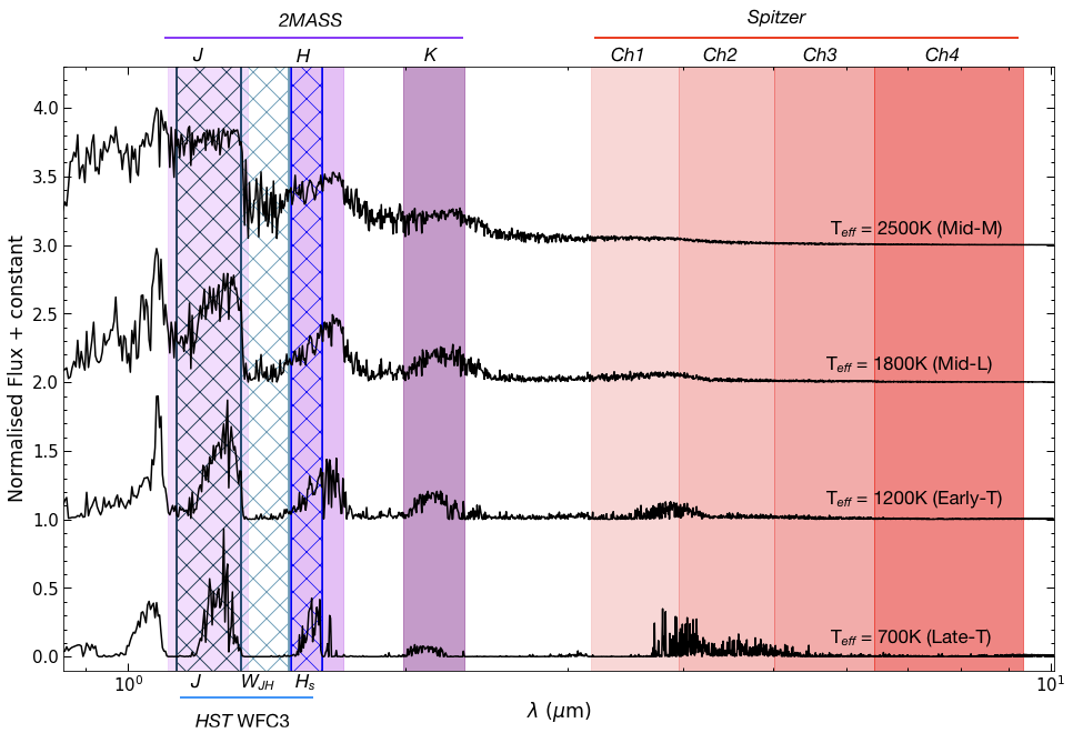
Figure 1: Model brown dwarf spectra, with photometric bands highlighted. In shades of red we have highlighted the position Spitzer’s channels 1–4. The three bands in shades of lilac are 2MASS bands J, H, and K; the HST G141 grism we used are in blue hatching, with each band we made from it hatched in a different shade of blue.

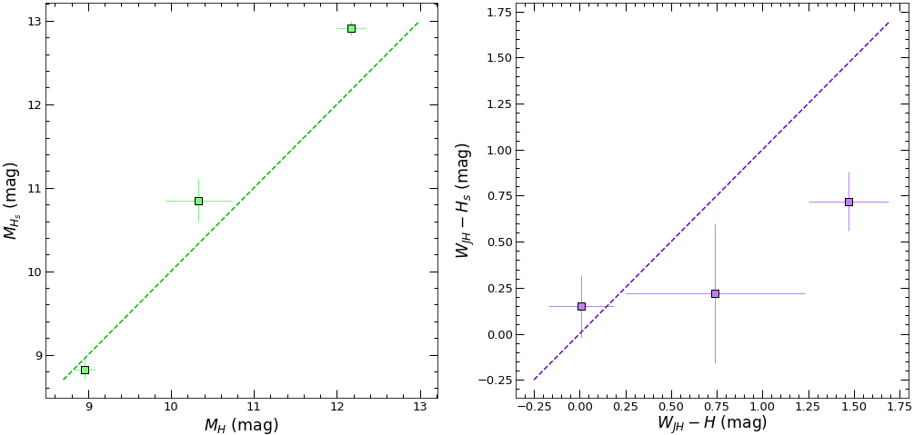
Figure 2: On the left panel we have show how H-short (H_s; obtained from WFC3 spectra) and H bands measurements cannot be assumed to be equivalent. We plot H_s absolute magnitudes vs. H absolute magnitudes for the three planets where these measurements exist (from left: WASP-12b, HAT-P-32b, WASP-43b). On the right panel we show ${\it W_{JH}}$ - H_s colours vs ${\it W_{JH}}$ - H colours for the same three planets. In both panels we show the position of the 1-1 line for ease of comparison.

The WFC3 instrument is most often used to search for signs of water in emission or transmission spectra due to a key water absorption feature at 1.4$\mu$m (Kirkpatrick, 2005). In order to test whether we could diagnose the presence or absence of water using a colour-magnitude diagram, we create a photometric band centred on the water feature between the J and H bands (W_JH-band hereafter) defined by integrating between 1.325 and 1.495$\mu$m. We therefore also add W_JH-band photometry for eleven planets to our database.

2.3 Assembling a brown dwarf comparisons sample

The beauty of a colour magnitude diagram is to enable simple comparison between population samples in a given wavelength space. A handful of objects on a colour-magnitude diagram by themselves do not allow us to infer much about these objects. Therefore, it is crucial that we have a large sample of well-studied objects to compare with our planets. As was done in Triaud et al. (2014), we make use of the detailed catalogue of near- and mid-infrared photometry of brown dwarfs produced by Dupuy & Liu (2012) to populate the background of our diagrams. Brown dwarfs are an excellent comparison sample as they overlap with exoplanets in temperature and radius, which leads to comparable luminosities (Triaud, 2014). For non standard bands, and for photometric bands that we defined, such as $W_{JH}$, there are no brown dwarfs catalogs we could use. We therefore synthetically create brown dwarf magnitudes and colours by integrating their spectra, which helps us populate the diagram and provide a comparison sample.

The SpeX Prism Library provides normalised near-infrared spectra of brown dwarfs spanning the wavelength range 0.8–2.5$\mu$m. These data are collected from the ground but are corrected for telluric absorption caused by water in the atmosphere (Rayner et al., 2003).

We integrated the SpeX spectra to produce a catalogue of photometry of 119 brown dwarfs. These were cross-referenced with the parallaxes provided by Dupuy & Liu (2012) in order to include distances in our catalogue. Our process of producing synthetic photometry is explained in Appendix A.2, along with how we validated our method. In Appendix F we have included a table of the photometry we computed in several near- and mid-infrared bands.

It is also important to verify whether exoplanet atmospheric models match observations. We produce synthetic photometry from atmospheric model spectra. In this paper we chose to use the publicly available model spectra produced by Mollière et al. (2015) as they cover a wide parameter space, most importantly carbon-oxygen ratios of 0.35 to 1.40; effective temperatures of 1000 to 2500K in 250K increments; and five metallicity values, ranging from -0.5 to 2.0. While we chose the Mollière models to demonstrate our code, it can adapted to use others as well. The data were processed using an adapted version of the code we used to produce magnitudes from Spex data.

2.4 Description of our Python Toolkit

We have produced a selection of Python tools which automate all of the data analysis methods described above. Data handling is packaged into three modules: Synth.py to produce synthetic photometry of brown dwarfs from SpeX spectra; Models.py to produce synthetic photometry from model exoplanetary spectra; and ExoCMD.py: a plotting module which computes planetary magnitudes and plots colour-magnitude diagrams. Users can interacts with the modules via a Jupyter Notebook; the code and the notebook can be accessed at https://github.com/gdransfield/ExoCMD.

Below we give a brief outline of the modules; more detailed information can be found in Appendix C, which also include a walkthrough tutorial.

2.4.1 Synth.py

This module provides a user with the flexibility to define bespoke photometric bands, in much the same way as we created our $W_{JH}$-band. New bands should be designed to coincide with interesting absorption features, which can be selected by inspection of brown dwarf spectra, or from line lists (e.g. Polyansky et al., 2018). Figure 1 shows model brown dwarf emission spectra (Baraffe et al., 2003; Allard et al., 2001) on which we have highlighted the 2MASS J, H, and K bands in lilac, along with Spitzer’s mid-infrared bands in shades of red. The hatched area corresponds to the G141 grism we used, with the light blue hatched area indicating the position of our $W_{JH}$-band. This plot shows how the 1.4$\mu$m water absorption widens and deepens with decreasing temperature.

It is important to bear in mind that a new band might not necessarily be useful for the full temperature range of brown dwarfs: the spectra of cooler objects is likely to be dominated by molecular species while hotter objects could have molecular, atomic or even ionised absorbers present. These changes are evident in the spectra shown in Figure 1, as well as the changing width of absorption features. Cooler objects are likely to need wider photometric bands to detect molecular features, whereas narrower bands are increasingly useful for the narrow absorption features seen in objects with higher temperatures.

Our Synth.py module contains seven built-in photometric bands, and all synthetic photometry will be produced in these bands along with a user-defined band. As well as the three 2MASS bands and our W_JH-band, we have included HAWK-I’s two narrow bands (NB1090 and NB2190) and Sloan’s z’-band.

While this module has been written with SpeX spectra in mind specifically, it can easily be adapted to work with any other brown dwarf spectra. The function outputs either a text file or a spreadsheet with photometry in the desired bands, along with spectral types and astrometric distances.

2.4.2 Models.py

The Models.py module computes photometry from Mollière’s model spectra. Although the code has been written with this particular set of models in mind, it can be used for any model spectra that are produced in physical units. The functions make use of the map provided by Mollière et al. (2015) to search for the spectrum which matches with the chosen parameters. The inputs required are constraints on metallicity, surface gravity, C/O ratio, effective temperature and host star spectral type. These constraints can be single values or lists of values; it is also possible to leave a parameter open which will result in all possible values being computed for that parameter. The two functions within the module output photometric magnitudes or colours respectively. There are eleven near- and mid-infrared bands built-in which can be called by name, and once again users can define bespoke bands if required.

2.4.3 ExoCMD.py

This module reads the planet database we have assembled and computes colours and magnitudes of exoplanets. There are five plotting functions which use these data to produce colour-magnitude diagrams.

The first plotting function (ExoCMD$\_$1) produces diagrams in the style of those presented in Triaud et al. (2014). We have added a keyword argument to this and all other plotting functions (adjusted) which when called will adjust the absolute magnitudes of the exoplanets to a size of 0.9R_J. This is to allow for a better comparison between planets, and to brown dwarfs. We chose this particular radius since typically brown dwarfs have a radius of $\approx$0.9R_J (Kirkpatrick, 2005) while hot Jupiters are more diverse in size. This only corrects the measurement with a simple translation up or down in absolute magnitude. See appendix B and Fig. 14 for an illustration of the effect of different adjustment factors.

The second and third plotting functions (ExoCMD$\_$2 and ExoCMD$\_$3) both show a polynomial to represent the mean trend of brown dwarfs in order to clarify and de-clutter the diagrams; this is especially valuable in colours where we now have many planets plotted. The polynomials are positioned using coefficients computed by Dupuy & Liu (2012). The key difference between the second and third plotting functions is a keyword argument (highlight) present in ExoCMD$\_$3 which greys out all planets except those called by name. This allows objects of particular interest to be highlighted when needed.

The remaining two plotting functions make use of our new comparison samples. They call the functions from Synth.py and Models.py in order to compute the necessary photometry for the bands requested. When using the model plotting function (ExoCMD$\_$model), the model atmospheres can be coloured according to any of the five model parameters (C/O ratio, metallicity, surface gravity, effective temperature, or host star spectra type); in the synthetic brown dwarf function (ExoCMD$\_$synth) the ultra-cool dwarfs are coloured according to spectral type.

All plotting functions additionally include the ability to plot the position of a blackbody of comparable radius to the objects plotted on the diagram.

3 Results

In the sections that follow, we present a selection of our colour-magnitude diagrams along with some of the key inferences we have been able to make from them. These are designed to be illustrative of how powerful it can be to view results for individual planets in context.

We begin with a brief explanation of how to read a colour-magnitude diagram, along with some of the terminology to expect. In Section 3.2, we show how a colour-magnitude diagram can allow us to select stand-out objects for rapid follow-up, and Section 3.3 outlines how inconsistency between colours of planets and brown dwarfs led us to investigate the absence of phosphine in irradiated objects. In Section 3.4 we demonstrate how a colour-magnitude diagram can be used to get a quick constraint on the C/O ratio.

3.1 Notes on Terminology

The x-axis of a colour-magnitude diagram is a colour index, calculated as the difference in magnitude between two photometric bands. It is conventional to subtract a longer wavelength magnitude from a shorter wavelength magnitude; this convention is observed throughout our paper.

In a conventional colour-magnitude diagram objects can therefore be compared in terms of their x-position on the plot: an object on the left hand side would be described as ‘bluer’ than one on the right hand side. This is due it having more flux, and therefore a higher magnitude, in the shorter, bluer wavelength than in the longer, redder wavelength. The converse is true of ‘redder’ objects. When describing the spread of objects on our colour-magnitude diagrams, we will therefore use the terms ‘bluer’ and ‘redder’ to refer to placements on the left and right hand sides respectively.

3.2 Outliers and Emerging Sub-populations

In this subsection, we go through a few examples on how colour-magnitude diagrams can be used to select target for additional observations, asking questions about patterns in the data, and diagnosing molecular signatures.

3.2.1 Identifying oddball systems and measurements

Figure 3 is a colour magnitude diagram made with our plotting function ExoCMD$\_$3. As we are comparing planets and brown dwarfs we have used the key word argument adjusted to scale the magnitudes to the size of a typical brown dwarf. On this plot we have highlighted two objects which are clear outliers, and one which is not.

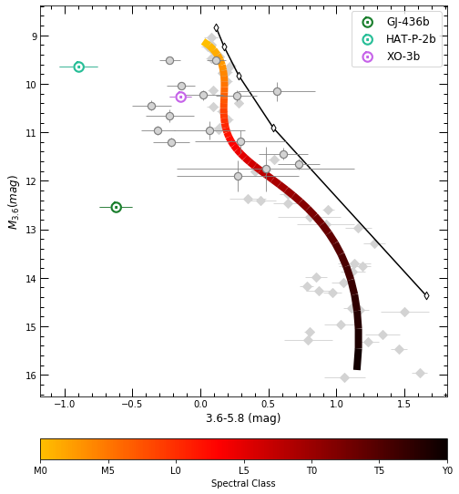
Figure 3: Colour-magnitude diagram in $M_{3.6}$ vs. [3.6 - 5.8$\mu$m] using our function ExoCMD_3. Planets are plotted as circles in the foreground, while brown dwarfs are grey diamonds in the background. Three planets have been plotted in colours in order to highlight their positions when compared with those in grey. The polynomial shows the mean position of the brown dwarf sequence and is coloured according to their spectral type. Planetary magnitudes have been scaled to a 0.9R_J object for better comparison with the brown dwarfs. The black line shows the position of a 0.9R_J blackbody with the white-filled diamonds showing the position of the blackbody at temperatures of 750K, 1750K, 2750K, 3750K and 4750K.

On the top left we have HAT-P-2b, a highly eccentric planet (e $\approx$ 0.5; Lewis et al., 2013)) that is speculated to have a dayside temperature inversion. In [3.6 - 4.5$\mu$m] it is consistent with both the L-Dwarf sequence and the mean position of other planets, which indicates that the 5.8$\mu$m flux is the one causing its very blue colour. The surprisingly shallow secondary eclipse in Spitzer’s Channel 3 was noted at the time of measuring, as it yields a brightness temperature $\sim$700K lower than the secondary eclipses measured in Channels 1, 2 and 4. If this low flux in the 5.8$\mu$m band is caused by processes unique to eccentric hot Jupiters, then it is possible that further eccentric systems will be similarly blue in this colour.

Further down on the same plot, we have GJ 436b. This object is also eccentric (e $\approx$ 0.14; Maciejewski et al., 2014b)) yet in this case the problematic flux is in the 3.6$\mu$m band. This is confirmed by its position on a M_5.8 vs [5.8 - 8.0$\mu$m] where it intersects exactly with the brown dwarf sequence.

GJ 436b is a hot Neptune with an equilibrium temperature of $\approx$700K (Turner et al., 2016), while HAT-P-2b is a hot Jupiter with an equilibrium temperature of 1540K (Pál et al., 2010). Following up on both of these objects will allow us to determine whether their blue colours in [3.6 - 5.8$\mu$m] are in any way caused by their eccentricity, and if so it could point to key population differences between Jupiter and Neptune-sized objects.

We have highlighted one other planet on Figure 3: XO-3b is the only other planet with a significant eccentricity (e significant $>0.1$) on this plot (e $\approx$ 0.28; Machalek et al., 2010)). The 3.6$\mu$m and 5.8$\mu$m fluxes for XO-3b have not been updated since 2010, and the values come from single eclipse measurements. When the 4.5$\mu$m flux was remeasured in 2014 by Wong et al. (2014) they calculated a deeper eclipse of 0.158$\%$ which differs by 2.1$\sigma$ from the original. This new eclipse depth was derived from 12 consecutive secondary eclipse events, and the mean variation between them of just 5$\%$ indicates no consequential orbit-to-orbit variation. XO-3b’s location within the population of circular planets throws a doubt on our initial hypothesis, an example on how a colour-magnitude diagram can be used.

Both of the HAT-P-2b fluxes were also calculated from single secondary eclipse events. For GJ 436b, the 3.6$\mu$m flux has been remeasured since the first observations of its thermal emission, but the 5.8$\mu$m has not; this latter value also came from a single eclipse event. Hansen et al. (2014) has claimed that these flux ratios measured from single events have low reproducibility and underestimated errors as they do not adequately account for instrument systematics. This throws into question the significance of results inferred from single-eclipse photometry.

A further stand-out system can be seen in Figure 4: on the far left with a colour of -0.9 we find WASP-65b. WASP-65b is one of the densest known hot Jupiters in its mass regime (R = 1.112R_J, M = 1.55M_J); it orbits in an area where inflated radii are the norm (a = 0.0334AU) yet it is denser than Jupiter itself (Gómez Maqueo Chew et al., 2013). It has been suggested that its uninflated radius could be evidence of the advanced age of the system, and that if this is the case, the contraction of its atmosphere could lead to changes in its temperature-pressure profile giving rise to unexpected spectral features. The measurements for WASP-65b also result from observations of a single eclipse event (Garhart et al., 2019).

These four planets are clear candidates for follow-up. While at first look, the data so far is indicative that eccentricity and density might cause an important difference in atmospheric properties in two cases, it is however more likely that a lack of repeated measurement is the root cause. Regardless of what the answer turns out to be, using a colour-magnitude diagram simplifies the process of target selection.

3.2.2 Planets near the T spectral class

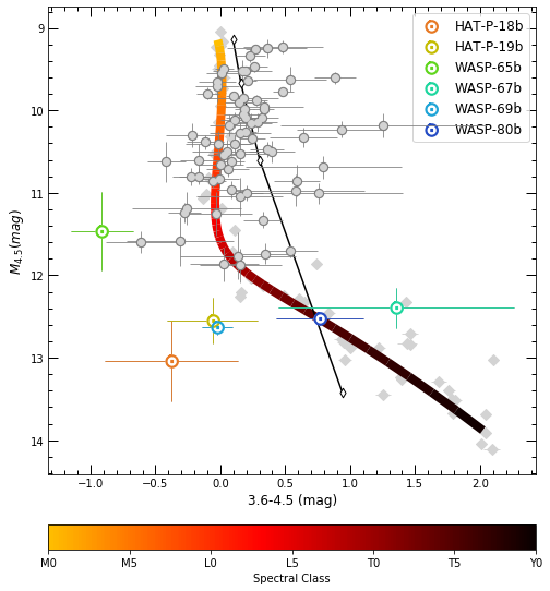
Figure 4: Colour-magnitude diagram in $M_{4.5}$ vs. [3.6 - 4.5$\mu$m] using our function ExoCMD_3. Planets are plotted as circles in the foreground, while brown dwarfs are grey diamonds in the background. Six planets have been plotted in different colours in order to highlight their positions when compared with those in grey. As before, the polynomial shows the mean position of the brown dwarf sequence and is coloured according to their spectral type. Planetary magnitudes have been scaled to a 0.9R_J object for better comparison with the brown dwarfs. The black line shows the position of a 0.9R_J blackbody with the white-filled diamonds showing the position of the blackbody at temperatures of 750K, 1750K, 2750K, 3750K and 4750K.

In Figure 4 we present a colour-magnitude diagram in M_3.6 vs. [3.6 - 4.5$\mu$m]. The five planets we have highlighted all have equilibrium temperatures of between 800-1000K, with HAT-P-18b and WASP-80b being the coolest of the set. Triaud et al. (2015) pointed out that WASP-80b was the first planet whose measured dayside flux fell in a position consistent with the L-T transition experienced by ultra-cool dwarfs between 1100-1500K. This transition is characterised by the emerging spectral signature of methane, which has its fundamental band at 3.3$\mu$m and is therefore detectable by Spitzer’s Channel 1. Triaud et al. (2015) suggested that this could be indicative that planets undergo a similar transition but at a lower temperature. The fact that we now have fluxes measured for HAT-P-18b which is comparable in temperature and radius (Wallack et al., 2019), yet is significantly bluer, indicates that perhaps this is not true of all cool exoplanets.

One way in which these two planets differ is in mass: WASP-80b is approximately three times more massive than HAT-P-18b (0.55M_J vs. 0.183M_J). Additionally, we find that WASP-67b, whose colour is also consistent with that of an early T-dwarf, is more than twice as massive as HAT-P-18b (Kammer et al., 2015). HAT-P-19b (0.292M_J) and WASP-69b (0.25M_J) fall between the others in both colour and mass. This is still too small a sample for a proper inference, however so far, there is an interesting indication in the transition from L to T class (CO to CH₄ chemistry) that increased mass might be correlated with a redder colour in [3.6 - 4.5$\mu$m].

This ties in well with the conclusions of Zahnle & Marley (2014), who showed that the temperature of transition from CO-dominated to CH₄-dominated atmospheres scales with gravity. As the densest of the five, WASP-80b also has the highest surface gravity which would point to a higher temperature to undergo the planetary version of an L-T transition.

An alternative interpretation for the range of colour that these planets cover might arise as differences in metallicity and C/O ratio. Kammer et al. (2015) sought to find a link between mass, metallicity and C/O ratio for cool exoplanets, with HAT-P-19b and WASP-67b included in their sample. They found a tentative link between the masses of cool planets and the ratio of 3.6$\mu$m and 4.5$\mu$m magnitudes, which is consistent with the suggestion that less massive planets have higher metallicities (Moses et al., 2013b). More recently, Wallack et al. (2019) found that for cool planets, extreme values of C/O ratio lead to big shifts in atmospheric chemistry, having large effects on the [3.6 - 4.5$\mu$m] colour. Our synthetic photometry of model atmospheres shows a very similar trend.

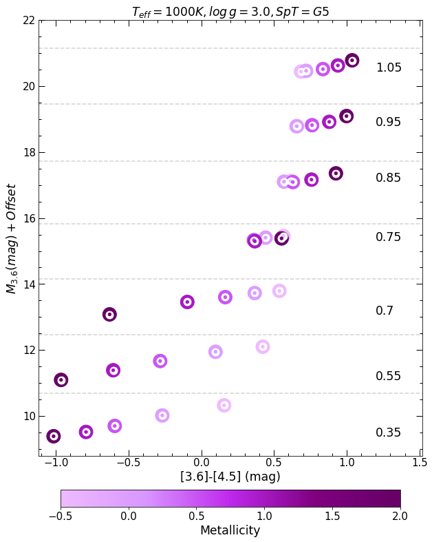
Figure 5: Colour-magnitude diagram of $M_{4.5}$ (plus an arbitrary offset) vs [3.6 - 4.5$\mu$m] using model spectra. The colours have been offset by -1 magnitudes (see Section 4.3 for an explanation of the motivation). Points are coloured according to their assigned metallicity and each row of points represents model spectral with a different C/O ratio, as detailed on the right-hand-side of each row.

Figure 5 shows a colour-magnitude diagram created using ExoCMD_model(). The Mollière spectra chosen correspond to a planet with T_eff = 1000K, log g = 3.0 and host star spectral type = G5. We found that this colour was not sensitive to host star spectral type, but showed some changes for values of log g $\geq$ 4. We can see that in this temperature regime, planets with a metallicity $>0$ (which we expect), experience a dramatic shift in colour with very small changes in oxygen abundance (between C/O = 0.7 and C/O = 0.85).

This shows that in principle, we could diagnose limits on both C/O ratio and metallicity for exoplanets under 1000K simply by measuring thermal emission in these two bands, and without extensive retrieval methods. For example the only objects with colours of 0.25 or lower are oxygen-rich ones. We also see that the very bluest colours only occur with a combination of oxygen-richness and high metallicity. Colours close to 1 indicate both high metallicity and a C/O $\geq$ 0.85.

At the time of writing this relationship is not yet calibrated. In Section 4.3 we outline the problem of model spectra which are not fully calibrated to real data. To account for this, the colours in Figure 5 have been offset by -1 magnitude. This offset is an approximation from inspection of the mean offsets in M_3.6 and M_4.5 as can be seen in Figure 11. We also note that the relationships outlined above are true for the Mollière model spectra used in this paper. An interesting next step would be to see if the same relationship holds for other model sets.

3.3 Identifying molecular Signatures

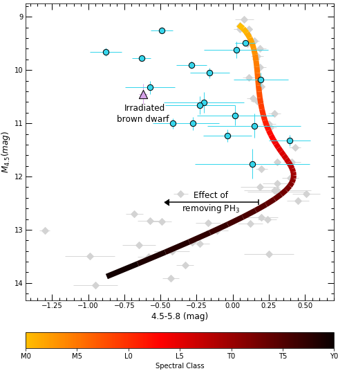
Figure 6: Colour-magnitude diagram showing the comparative blueness of planets with respect to brown dwarfs of similar brightness. Planets are plotted as blue circles in the foreground, while brown dwarfs are grey diamonds in the background. Once again, the polynomial shows the mean position of the brown dwarf sequence and is coloured according to their spectral type. The planetary absolute magnitudes have been scaled to a size of 0.9R_J for better comparison with brown dwarfs. Additionally, we have plotted the position of the irradiated brown dwarf WD0137-349B as a lilac triangle. The black arrow indicates the effect on this colour of removing phosphine.

One interesting prospect for colour-magnitude diagram would be their ability to diagnose the presence of certain molecules, which would help setting up certain retrieval schemes.

A plot similar to Figure 6 appeared in Triaud et al. (2014), who highlighted a large discrepancy between the colours of brown dwarfs and hot Jupiters. Even with our improved distance measurements and absolute magnitudes adjusted to 0.9R_J, we can clearly see that planets are systematically bluer than brown dwarfs. This is in contrast with most near- and mid-infrared colour-magnitude diagrams where the planets are largely consistent in both colour and magnitude with the L-dwarf sequence (see Appendix E for up-to-date colour-magnitude diagrams). In Triaud et al. (2014) we suggested that the discrepancy in [4.5 - 5.8$\mu$m] could perhaps be explained by an additional absorber within the 4.5$\mu$m band, present for the brown dwarfs but not for the exoplanets. We reached this conclusion because 5.8$\mu$m measurements of exoplanets appear consistent with brown dwarfs’.

An important difference between brown dwarfs and hot Jupiters is that while brown dwarfs are self-luminous, hot Jupiters are irradiated objects. We searched the literature to find out what irradiation could produce in relation to the 4.5 $\mu$m band. We identified phosphine, PH₃, as a molecule present within brown dwarf atmospheres, but most likely absent in hot Jupiters (due to photolysis), as the cause of the discrepancy.

Phosphine has a strong absorption feature at approximately 4.3$\mu$m (Sharp & Burrows, 2007) and is identified as the most likely Phosphorus-carrying gas in the observable atmospheres of hot T-dwarfs and cool L-dwarfs, with temperatures in the range 1000K - 1400K (Visscher et al., 2006). Visscher et al. (2006) also notes that while in the atmospheres of warmer L-dwarfs PH₃ may be replaced by other phosphorus-bearing species, it may still be possible to detect the 4.3$\mu$m PH₃ feature if it can be distinguished from the 4.5$\mu$m CO feature. However, PH₃ is highly susceptible to irradiation (Sousa-Silva et al., 2019), and if present in the atmospheres of hot Jupiters, we expect it to be photodissociated and therefore not detectable. This would also then be true of other highly irradiated objects such as brown dwarf secondary to high-mass or high-temperature primaries.

We sought to verify our hypothesis by searching for an irradiated brown dwarf with an eclipse measurement in the bands that we considered. There is only one such object to our knowledge, WD0137-349B (Casewell et al., 2015). This object is part of a white dwarf - brown dwarf binary and as such its dayside is subject to high levels of irradiation. We plot WD0137-349B’s irradiated side on Figure 6 (Casewell et al., 2015). Its position on the colour-magnitude diagram is more consistent with the most irradiated exoplanets rather than the ultra-cool dwarfs. We interpret this as indication that irradiation is likely the cause of a higher than usual flux in the 4.5 $\mu$m channel. Since phosphine does absorb in that particular band, and is expected to be within brown dwarfs’ atmospheres, but not within hot Jupiter, we deduce that a lack of phosphine may provide a good explanation for the 4.5 $\mu$m measurements.

To further investigate whether phosphine can have the effect we thought, we used model spectra of GJ 504b produced with and without PH₃ present (Baudino et al., 2017). We integrated these spectra and found that the removal of PH₃ from the atmosphere causes a blueward shift of 0.65 magnitudes in [4.5 - 5.8$\mu$m]. We have added an arrow of this size to Figure 6 to illustrate the impact of PH₃ in this colour, which has an amplitude consistent with the difference between brown dwarfs and hot Jupiters, and between the irradiated brown dwarf WD0137-349B and its field brethren.

One further interesting feature of Figure 6 is that the amplitude of the colour offset between brown dwarfs and hot Jupiters increases with decreasing absolute magnitude (i.e. increasing equilibrium temperature). Equilibrium temperature is obviously related with insolation. If the bluer colours of planets are caused by the photodissociation of PH₃, then higher levels of insolation would be expected to lead to higher PH₃ depletion.

Could it be something else? Madhusudhan & Seager (2011) describe how Spitzer fluxes, and therefore our colours, can be interpreted based on knowledge of the location of spectral features of the key absorbers present in an atmosphere. Most notably, they state that these interpretations are based on the assumption that H₂O, CH₄, CO and CO₂ are the four dominant molecules in all Spitzer bands. Of these four, CO and CO₂ both have strong absorption features in the 4.5$\mu$m channel, so low fluxes in this band are usually attributed to one or both of these molecules. However, thermal equilibrium predicts that both brown dwarfs and hot Jupiters should have most of their atmospheric carbon locked into CO in this temperature regime. We therefore return to our ‘additional absorber’ hypothesis.

An alternative explanation is to invoke thermal inversions in the vast majority of the hot Jupiters depicted in Figure 6. With such an inversion, CO would be in emission and increase the flux in the 4.5$\mu$m band. However, as we discuss 4.2, planets with compelling evidence for a thermal inversion are scarce, and their existence is doubted by several authors.

One other possibility worth considering is the effect of clouds. Clouds are believed to be the cause of the significant colour change seen in brown dwarfs close the L-T transition in near and mid-infrared colours (Patten et al., 2006), as the disappearance of silicate and iron condensates reveals atmospheric methane absorption (Triaud et al., 2014). It is unclear as yet whether similar colour changes in exoplanets could also be caused by clouds since very few planets corresponding to a T spectral class have been measured. In transmission spectroscopy, spectral features can present lower amplitudes than expected due to the presence clouds and haze opacities (Wakeford & Sing, 2015), which can lead to incorrect abundances being inferred. This is less the case when considering secondary eclipse data, as the daysides of planets as the spectrum probes at a higher altitude (Madhusudhan, 2018). Nevertheless, better understanding of the role of clouds and hazes in exoplanetary atmospheres is needed to rule this out as a contributing factor since difference in irradiation and gravity between brown dwarfs and hot Jupiters might produce differing cloud coverage, altitude, and dynamics. From visual inspection of Fig. 18, and particularly of Fig. 19, we note that irradiated hot Jupiters and field brown dwarfs do follow a similar behaviour in the near-IR, over the L-type range, where clouds are thought to dominate brown dwarf atmospheres.

3.4 Seeking to constrain the C/O ratio with colour-magnitude diagrams

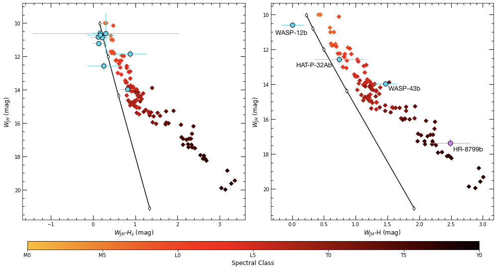
Figure 7: Colour-magnitude diagrams of $M_{W_{JH}}$ vs. [$W_{JH}-H$] made using our plotting function ExoCMD_synth. Planets are plotted as blue circles with their magnitudes scaled to a 0.9R_J sized object to allow better comparison with the brown dwarfs. Brown dwarfs are plotted in the background as diamonds coloured according to spectral type. The black line shows the position of a 0.9R_J blackbody, with the white-filled diamonds highlighting the position at temperatures of 1000-5000K in steps of 1000K. Left panel: $M_{W_{JH}}$ vs. [$W_{JH}$-$H_{s}$]. We note that in this colour planets are significantly less spread out in colour. Right panel: $M_{W_{JH}}$ vs. [$W_{JH}-H$]. HR8799b is highlighted in lilac as its photometry was taken with direct imaging rather than secondary eclipse observations (Rajan et al., 2015; Marois et al., 2008).

In Figure 7 we present colour-magnitude diagrams featuring our new W_JH band, made with our ExoCMD$\_$synth() function. On the left-hand panel we have plotted nine of the planets which have low resolution spectra measured with HST, combining $W_{JH}$ photometry with H_s). We include this as there are significantly more planets available than those with H-band photometry, but we see that their positions are shifted in colour with respect to the left panel. On the right-hand panel we have plotted three planets: from brightest they are WASP-12b, HAT-P-32Ab, WASP-43b. We computed the brown dwarf photometry for both panels with our Synth.py code, and we computed photometry for the three planets by integrating low resolution emission spectra measured with the Hubble Space Telescope’s G141 grism.

We have yet to identify a colour index where objects with confirmed water detections are easily distinguishable from those without, however we can see that three objects in 7 are widely spread in colour. Incidentally, all three of these planets have firm detections of water using these data.

The H-band is centered on 1.6$\mu$m and has a prominent CH₄ absorption feature, and a slightly weaker CO feature (Sharp & Burrows, 2007), while the W_JH-band is dominated by water absorption. These four molecules are related by the following net equilibrium equation, as described in Madhusudhan (2012):

$$\ce{CH4+H2O<=>T[T$\ga$1000K][T$\la$1000K]CO+3H2}.$$ (2)

In objects cooler than 1000K the left hand side of the equation is favoured and methane is the dominant carbon-bearing molecule. For objects hotter than 1000K, carbon is found mainly in the form of carbon monoxide. However, if a hotter atmosphere is also oxygen rich, we would expect the excess oxygen to react with the H₂ to form water. This indicates that C/O ratio should be the biggest indicator of both [W_JH - H] colour and water abundance: more excess oxygen will cause more water to be produced. This will deepen the absorption at 1.4$\mu$m leading to increased W_JH magnitude, and therefore a redder colour. This is consistent with the retrieved water abundances for WASP-12b and WASP-43b by Line et al. (2014): WASP-43b’s abundance was found to be greater than WASP-12b’s by a factor of 10³.

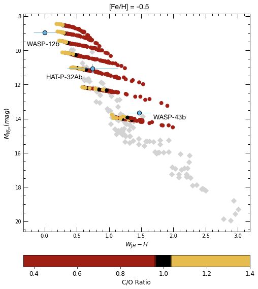
Figure 8: Colour-magnitude diagram of $M_{W_{JH}}$ vs. [$W_{JH}-H$], plotted using our function ExoCMD_model. The following parameters were entered for the model: $T_{\rm eff}$ = 1000 – 2500K, log g = 2.3, 3.0, 4.0 and 5.0, SpT = G5, and [Fe/H] = -0.5. Points have been coloured according to C/O ratio in order to highlight the differences between carbon- and oxygen-rich atmospheres. Brown dwarfs are plotted in the background as grey diamonds.

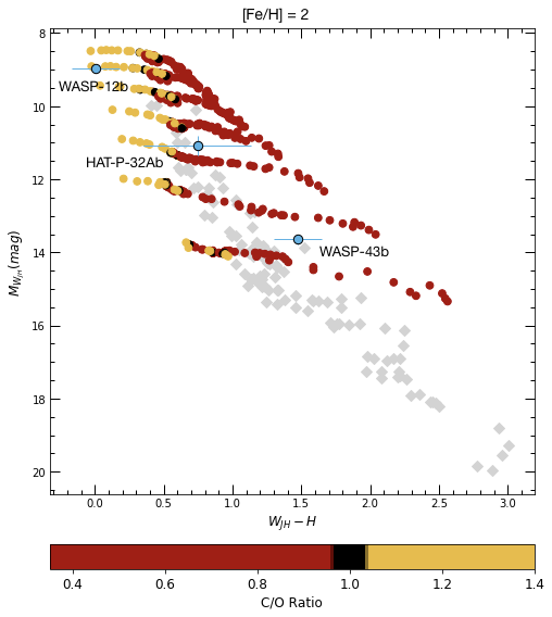
Figure 9: Colour-magnitude diagram of $M_{W_{JH}}$ vs. [$W_{JH}-H$], plotted using our function ExoCMD_model. The following parameters were entered for the model: $T_{\rm eff}$ = 1000 – 2500K, log g = 2.3, 3.0, 4.0 and 5.0, SpT = G5, and [Fe/H] = 2. As before, points have been coloured according to C/O ratio in order to highlight the differences between carbon- and oxygen-rich atmospheres. Brown dwarfs are plotted in the background as grey diamonds.

Figures 8 and 9 are colour-magnitude diagrams featuring Mollière model atmospheres. Both have been plotted for four values of log g from 2.3 to 5.0, seven values of effective temperature from 1000–2500K, and a host star spectral type of G5. Figure 8 features atmospheres with a metallicity of -0.5, while in Figure 9 we have assigned a metallicity of 2.0. The models have been coloured according to their C/O ratio.

We can see from Figure 8 just how much [W_JH - H] colour is affected by the C/O ratio, and for two of the planets here plotted we can attempt to infer whether they are consistent with oxygen- or carbon-rich model spectra.

Within its uncertainties, WASP-43b colours and magnitudes are consistent with an oxygen-rich atmosphere for all values of surface gravity, and retrievals of its metallicity have found it to be 0.3–1.7 $\times$ Solar (Kreidberg et al. (2014), Stevenson et al. (2017)). Therefore it is best matched by Figure 9, and we can see that its colour is indicative of an oxygen-rich atmosphere. This is in agreement with the upper limit set by Benneke (2015), and indeed with the recent retrieval by Irwin et al. (2019).

In contrast, WASP-12b’s eclipse measurements coincide with the carbon-rich model atmospheres for both extremes of metallicity and all values of surface gravity. This is in agreement with Madhusudhan et al. (2011a) who found C/O $\geq$ 1 using Spitzer secondary eclipse data. This has since been contested, with Kreidberg et al. (2015) finding that the atmosphere was best fit by C/O $\approx$ 0.5 using HST transit data, but omitting Spitzer transits due to instrument systematics. Benneke (2015) also retrieved an oxygen-rich atmosphere with C/O < 0.9 for WASP-12b, even though analysis of previously unpublished Spitzer measurements by Stevenson et al. (2014b) had confirmed the original findings. We need a better understanding of the physical processes that lead to WASP-12b appearing consistent with carbon-rich model atmospheres; additionally, in order to confirm this consistency we need to ensure that the models are well calibrated to the data in this colour. See section 4.3 for more detail.

We were unable to find a constraint on HAT-P-32Ab’s C/O ratio in the literature, and due to the large errors on the colour we find that it is equally compatible with carbon-rich and oxygen-rich model atmospheres.

4 Discussion

In the following sections we discuss the implications of our results, placing them in the context of unexplained low fluxes and exciting upcoming missions.

4.1 Phosphine

The recently updated line list for phosphine published by Sousa-Silva et al. (2015) puts us in a favourable position to identify planets where this gas may be present. Over the lifetime of Spitzer there have been many unexplained low fluxes measured in Channel 2. In this section we speculate about the impact that phosphine may have for a number of eclipse measurements, and planetary environments.

The absence of PH₃ on the daysides of hot Jupiters due to high levels of irradiation would not preclude the possibility of its presence on the cooler and less irradiated nightsides. One such candidate is HD 189733b which has a puzzlingly low nightside flux in 4.5$\mu$m (Knutson et al., 2012; Steinrueck et al., 2019). The lack of irradiation on the nightside may have prevented photodissociation of the molecule, and the lower temperatures would be indicative of PH₃ accounting for most of the atmospheric phosphorus budget (Visscher et al., 2006). Even if photodissociated on the dayside, Phosphorus might recombine into phosphine on the nightside, after being transported by winds.

Alternative explanations were made for this low 4.5${\rm\mu}$m flux. For instance, Carbon monoxide (CO) also has a deep absorption feature in the 4.5$\mu$m band (Sharp & Burrows, 2007), and when the phase curve for HD 189733b was first observed in Spitzer’s Channel 2, the low nightside flux was attributed to this molecule (Knutson et al., 2012). It was initially thought that non-equilibrium chemistry would be able to explain the fact that CO was the main carbon-bearing molecule, despite the low temperature. However, recently (Steinrueck et al., 2019) showed that this is not the case: disequilibrium processes alone cannot account for the low fluxes in Spitzer’s Channel 2 as excess CO is balanced by a drop in H₂O.

Two other hot Jupiters with similarly low 4.5$\mu$m nightside fluxes are HD 209458b (Zellem et al., 2014) and WASP-43b (Stevenson et al., 2017). Here too, models predict they should be significantly brighter than they are in Spitzer’s Channel 2, as equilibrium chemistry would point to CH₄ being the main carbon-bearing molecule on the cooler nightside. The inclusion of PH₃ in these models could revise our understanding of these planets.

Considering PH₃ in atmospheric composition may additionally help to shed light on surprisingly shallow 4.5$\mu$m secondary eclipses measured on the daysides of far cooler planets. GJ 436b has had consecutive non-detections in Spitzer’s Channel 2 (Stevenson et al., 2010; Lanotte et al., 2014; Morley et al., 2017), pointing to a CO/CH₄ ratio which is considerably higher than equilibrium chemistry would predict for an object of this temperature ($\approx$700K (Turner et al., 2016)). ‘Additional absorbers’ have been postulated for GJ 436b by Morley et al. (2017) in order to resolve the apparent low flux in this wavelength, and PH₃ could be that absorber.

A similar non-detection in the 4.5$\mu$m band for WASP-29b prompted claims of possible non-equilibrium abundances of CO (Hardin et al., 2012). WASP-29b is a Saturn-sized object with an equilibrium temperature of 980K; PH₃ could yet again provide an explanation for this excess absorption. Most recently, GJ 3470b had a minute 4.5$\mu$m flux measured by Benneke et al. (2019); this is a low metallicity, sub-Neptune sized planet with an equilibrium temperature of approximately 600K. Equilibrium chemistry once again points to Methane accounting for most of its atmospheric carbon budget, and phosphine as a convenient molecule to explain the observations.

4.2 Upcoming Missions

The James Webb Space Telescope (JWST) is scheduled for launch in 2021 and is intended as a successor to the Hubble Space Telescope. A recent simulation of JWST spectra by Wang et al. (2017) assessed the detectability of PH₃ by the telescope’s NIRCam instrument and found that it could be detectable in emission spectra for objects of around 500K, and in transmission spectra for objects cooler than 1000K. Although they concluded that for objects of 1000K or more PH₃ could not be resolved with a secondary transit, we speculate that objects of intermediate temperatures, such as GJ 436b, might have detectable PH₃ due to their low 4.5$\mu$m fluxes. Additionally, the MIRI instrument will cover the wavelength range of Spitzer’s 5.8$\mu$m band (Rieke et al., 2015); we can therefore use photometry taken in this instrument’s Channel 1 to add objects highlighted in Figure 4 to our PH₃ diagnostic colour-magnitude diagram. The extent to which these objects are offset from the brown dwarfs will indicate whether we should follow up on them using NIRCam to search for PH₃.

While in this paper we propose that phosphine could be responsible for some of the differences in colour seen between hot Jupiters and brown dwarfs, this is not without its issues. Phosphine is hard to distinguish from CO in hotter objects, and in some of the coolest brown dwarfs, where PH₃ is expected to dominate the 4.5 $\mu$m band, the evidence for its presence is still scarce. JWST will therefore also allow us to explore the spectra of brown dwarfs in more detail in order to confirm the presence or absence of phosphine in these objects. The first M-band (4.5-5.1 $\mu$m) spectrum of WISE 0855, the coldest known brown dwarf, rather surprisingly did not reveal evidence of phosphine absorption; this despite being very similar to Jupiter in other respects (Skemer et al., 2016). This was interpreted as evidence that WISE 0855 might not share Jupiter’s turbulent vertical mixing, which is responsible for the large abundances of PH₃ present in its observable atmosphere. Morley et al. (2018) later presented an L-band (3.4-4.14 $\mu$m) spectrum of WISE 0855; this too lacked the expected footprint of PH₃. This work was recently extended to six other brown dwarfs in the temperature range 250-750K, and phosphine absorption was still not clearly present in any of them (Miles et al., 2020). The authors do point out that the wavelength ranges where phosphine would be most detectable (the end of the L-band and start of the M-band) coincide with the lowest signal-to-noise in their data. It is also worth noting that the centre of the phosphine absorption feature is at 4.3 $\mu$m, which falls precisely in the gap between the L and M-bands. Fortunately, JWST’s NIRCam will have both the spectral coverage and the resolution to shed new light on this mystery.

JWST will also be equipped with a Near Infrared Spectrograph (NIRSpec) Dorner et al. (2016) with wavelength coverage of 0.6–5.3$\mu$m. We will therefore be able to use our photometry tools to make diagnostics about the planets’ atmospheres, using colour-magnitude diagrams by integrating JWST spectra. While this does not replace a full atmospheric retrieval, the goal will be to identify objects that appear to be, for instance carbon-rich, or outlying the main population for one reason or other, and propose them for a more detailed follow-up as was simulated by Schlawin et al. (2018).

The C/O ratio is essential to our understanding of how and where a planet formed (e.g. Öberg et al., 2011; Madhusudhan et al., 2011b; Madhusudhan, 2012; Madhusudhan et al., 2017). It can also tell us whether or not a thermal inversion is likely, as carbon-rich atmospheres favour low abundances of the two molecules thought to be producing inversions (Madhusudhan & Seager, 2011): TiO and VO (Fortney et al., 2008). Additionally, the C/O ratio can give an indication about the habilitability of a planet (Johnson et al., 2015), as a C/O$\geq$1 causes depletion of water, even if the planet is within the habitable zone.

The detailed spectra which JWST will be capable of producing will also help to shed light on the atmospheres of controversial planets such as WASP-12b. This planet is predicted to have a stratosphere due to its very hot temperature (Hebb et al., 2009); however, so far TiO and VO have not been detected with any certainty as measurements of eclipse depths in relevant bands have been inconsistent (Sing et al., 2013; Hooton et al., 2019). Most recently, there has been close scrutiny of the orbit of WASP-12b due to the changing transit mid-points; the data now available points to orbital decay over apsidal precession (Bailey & Goodman, 2019; Yee et al., 2020). There is also no consensus as yet on whether WASP-12b is carbon- or oxygen-rich: detections of water in transmission (Kreidberg et al., 2015) point to an oxygen-rich atmosphere, yet the shallow 4.5$\mu$m eclipse depth indicates CO in absorption rather than emission (Stevenson et al., 2014b).

If WASP-12b does have a thermal inversion caused by TiO, VO or another mechanism, then its position on Figures 8 and 9 might be misleading. Parmentier et al. (2018) explains how the dissociation of H₂O in the atmospheres of ultra-hot Jupiters with stratospheres leads to free hydrogen atoms capturing electrons. The resulting H^- ions produce absorption features in the same spectral region as H₂O, which can lead to confusion when interpreting low-resolution spectra in the 1.4$\mu$m band. In the era of JWST, we will be able to refine our interpretations of positions of ultra-hot Jupiters on our colour-magnitude diagrams in order to improve our use of them as diagnostic tools.

Looking further into the future, Ariel is planned for launch in 2028. Like JWST, it will be equipped with near- and mid-infrared spectrographs which will allow for detailed atmospheric characterisation. In particular, the Near Infrared Spectrograph (NIRSpec) covers the wavelength ranges of the H and W_JH bands which will enable us to get an initial diagnostic on the C/O ratio, while the Ariel InfraRed Spectrometer (AIRS) covers the 1.95–7.8$\mu$m range allowing us to choose targets to follow-up on to find PH₃.

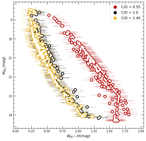
Figure 10: Exoplanet populations with different C/O ratios can be distinguished if they exist. Here, we show simulations of the Ariel yield on a colour-magnitude diagram of $M_{W_{JH}}$ vs. [$W_{JH}-H$], plotted using our function ExoCMD_model. The closest matching model spectrum was selected for each planet on the target list, and plotted with a C/O value of 0.55, 1.0 and 1.40 to show the spread in colour. Points are coloured according to C/O ratio.

Edwards et al. (2019) recently produced a list of potential targets for Ariel along with their radii and equilibrium temperatures. We searched the literature for their surface gravities, host star metallicities and host star spectral types; we were able to find all three data for 210 of the potential targets. We used this information to select the most appropriate model spectrum from Mollière et al. (2015) and plotted them on a M${}_{W_{JH}}$ vs [W_JH-H] colour-magnitude diagram, assigning C/O ratio values of 0.55, 1 and 1.40. As the Mollière models are only available in 250K increments, we interpolated the magnitudes in order to get a more realistic spread of colours. We did not have access to the Ariel Radiometric Model (Mugnai et al., 2019) to estimate the errors on the magnitudes; we therefore assigned an error of $\pm 0.1$ mag. This choice was not arbitrary; when computing photometry from HST/WFC3 spectra, the data with resolution comparable to what Ariel will produce yielded signal-to-noise ratio of 10, equivalent to a tenth of a magnitude. We present the resulting plot in Figure 10.

While the values for surface gravity, metallicity and host star spectral type had to be rounded to fit the model grid, we can see that objects with C/O ratio $\geq$1 are distinguishable from oxygen-rich objects.

A recent paper by Melville et al. (2020) also attempted to use colour-magnitude and colour-colour diagrams to constrain the atmospheric properties of exoplanets. In this paper, model spectra were computed using VSTAR (Versatile Software for Transfer of Atmospheric Radiation) (Bailey & Kedziora-Chudczer, 2012) for a range of values of metallicity, log g and C/O ratio. Model atmospheres were then compared with hot Jupiters in near- and mid-infrared colours using photometry in $JHK_{s}$-bands and Spitzer’s channels 1 and 2. While planets were seen to cluster around solar values of C/O and metallicity, no definitive constraints were found as the error bars were too large.

4.3 Model Calibrations

Our C/O ratio diagnostic tools rely on the availability and reliability of model spectra. We chose to use the models presented in Mollière et al. (2015) as they covered a very wide parameter space and were publicly available. However, those models have limitations which impact the validity of our inferences.

The first limitation we find is simply the range of temperatures available. JWST and Ariel will both observe objects cooler than 1000K in more detail than ever before, and in order to use models to characterise these objects it is essential that we have model spectra in this temperature range.

The second limitation comes from the quality of the fit for different wavelengths. In their paper, Mollière et al. (2015) showed a comparison between their retrieved model spectrum for HD-179833b and the many thermal emission measurements available for this planet. They showed that Spitzer photometry at 8$\mu$m was well fit by their model, while the shorter wavelength channels were not. They also showed that while the pattern for the HST data was well fit, the measured eclipse depths were larger than those retrieved by the model.

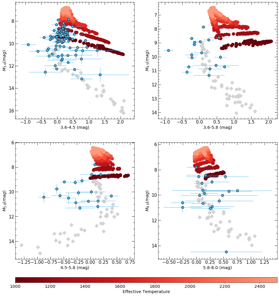
Figure 11: Colour-magnitude diagrams in Spitzer channels 1–4 showing how models do not reproduce planetary properties well. Planets are plotted as blue circles in the foreground, while brown dwarfs are grey diamonds in the background. Planetary magnitudes are not adjusted as we want to show how closely they match with model atmospheres. Model planetary magnitudes are plotted as edgeless circles, coloured according to effective temperature.

We illustrate the disparity between the measured data and the model spectra in IRAC channels in Figure 11. It is clear from these plots that there is a systematic offset in all four Spitzer bands when we compare with a large enough sample. But this also demonstrates that colour-magnitude diagrams, and indeed our tools to produce them, are especially valuable to modellers to validate their model spectra. It is also a cautionary note since similar spectra used for retrieval would be unlikely to lead to correct abundances.

The completeness of the chemistry included into the models impacts the outcome of retrievals. In particular, Baudino et al. (2017) showed how an incomplete line list for PH₃, let alone its exclusion from models altogether, can lead to this crucial molecule not being detected at all. We would also need oxides of titanium and vanadium included in radiative transfer calculations in order to ensure that possible thermal inversions are explored.

5 Conclusions

In this paper we have presented a public Python toolkit for the plotting of near- and mid-infrared colour-magnitude diagrams. To demonstrate the functionality of the toolkit, and the usefulness of colour-magnitudes of transiting exoplanets, we have presented a selection of our newly plotted diagrams. From these we have identified some trends:

• Two objects (HAT-P-2b and GJ 436b) are very blue in [3.6$\mu$m - 5.8$\mu$m] colour. Despite the fact that for each of these planets the blue colour is caused by excess emission in different bands, what they have in common is high eccentricity. Further follow-up could reveal if their colours are related to their eccentricity, and if so, whether mass and eccentricity are linked to cause excess brightness in different photometric bands. Remeasuring the mid-infrared photometry of XO-3b will also confirm why this planet does not share the blue colours of HAT-P-2b and GJ 436b.

• Objects cooler than 1000K show a wide spread in colours in [3.6 - 4.5$\mu$m] colour, which could be attributed to mass, metallicity and C/O ratio. By comparing the positions of five planets to the colours of model atmospheres we find that for C/O ratio $\geq$0.85, high metallicity causes reddening. At C/O ratios $\leq$0.75, increasing metallicity causes increasing blueness. For the planets we plotted, we also find that increasing surface gravity corresponds to redder colours.

• We attribute the comparative blueness of planets in [4.5 - 5.8$\mu$m] colour to missing PH₃, which absorbs prominently in the 4.5$\mu$m band. Field brown dwarfs in this temperature range could be expected to have Phospine account for most of their atmospheric phosphurus budget, yet as PH₃ is susceptible to photolysis by ultraviolet radiation, we believe it is feasible that hot and ultra-hot Jupiters would be missing this absorber. We propose that PH₃ might have been overlooked to explain several low 4.5$\mu$m fluxes, including on the dayside of GJ 436b and the nightside of HD 189733b.

• The [W_JH - H] colour index can be used to diagnose the C/O ratio of exoplanets. Magnitude increases in the W-band with increased water absorption, which we attribute to lower C/O ratios. From its position on a M_W vs [W_JH - H] diagram, we find WASP-12b to be carbon-rich.

In order to further refine constraints which derive from comparisons with model magnitudes, model spectra need to be calibrated to real data to the greatest extent possible. Our colour-magnitude diagrams are very well suited to this purpose.

With the launch of JWST now close, our colour-magnitude diagrams will be an invaluable tool for target selection in this new era of exoplanet atmospheric characterisation. Additionally, ESA’s Ariel mission will enable us to begin to study populations as a whole. Here colour-magnitude diagrams can prove essential to identify various sub-population, and to select targets from Tier 1 observations to the more detailed and higher signal-to-noise Tier 2 & 3.

Data Availability

The data used in this article are available in tables in the appendices of the article, and on Github together with the Python toolkit developed for this article at https://github.com/gdransfield/ExoCMD.

Appendix A recovering magnitudes

A.1 Host star magnitudes in new bands

Where a host star apparent magnitude was not available, we made use of standard spectra from the Pickles Atlas. In order to calculate the magnitudes of the parent stars, we began by searching exoplanet.eu (Schneider et al., 2011) for the spectral type of the host star. We acquired the Pickles spectrum corresponding to the parent star’s spectral type; we then integrated the flux in 2MASS J, H and K bands. For all magnitudes computed in this paper, we use the Vega-Magnitude system, setting its apparent magnitude to zero in all bands.

In order to compute Vega’s flux in J, H and K we obtained Kurucz’s high resolution spectrum which we then integrated in all three bands. Finally, we recovered H and K magnitudes from J, J and H from K, and J and K from H. Where the spectral type of the parent star was not certain in the literature, we chose the spectrum which was a best fit in terms of temperature and recovered magnitudes. We present one-to-one plots of these recovered magnitudes in Figure 12.

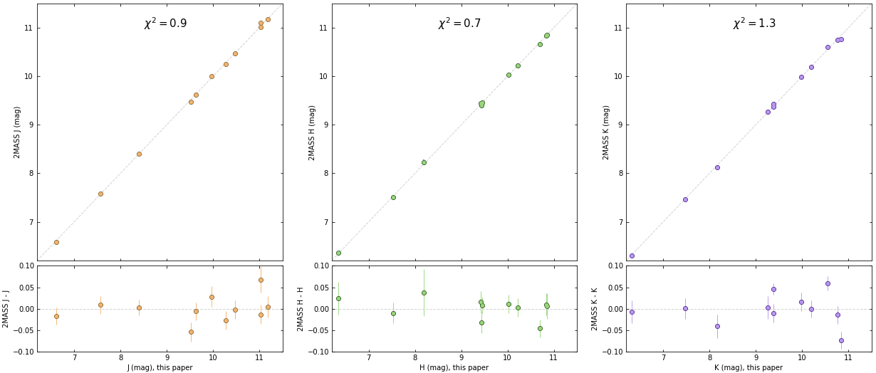
Figure 12: 2MASS magnitudes of parent stars from the literature compared with our recovered mags using standard spectra from the Pickles Atlas.

A.2 Brown dwarf magnitudes from SpeX spectra

We initially downloaded all 597 files available containing spectra for objects spanning the M to T spectral classes. 2MASS J, H and K magnitudes were provided for the majority of them; we discarded any data where they were missing. We calculated apparent magnitudes using Vega as a reference once again, integrating the Kurucz spectrum in each band. In order to test the validity of our method, we first combined the integrated Vega flux with the provided 2MASS magnitudes of each star to recover synthetic J, H and K magnitudes for the brown dwarfs. As each of the spectra are provided normalised, an important step in the determination of the magnitudes was to calculate a scale factor from each. These scale factors were determined by computing the band-integrated flux for each star in the same units as Vega’s flux, working backwards with each of the 2MASS magnitudes:

$$\centering F_{bd}=F_{vega}\times 10^{\frac{2MASS\,(mag)}{-2.5}},\@add@centering$$ (3)

where F_bd is the band-integrated brown dwarf flux in Vega’s units, F_vega is Vega’s band-integrated flux, and 2MASS (mag) is the 2MASS J, H or K magnitude of the brown dwarf. Dividing these fluxes by those obtained by integrating the spectra of the brown dwarfs yielded the required scale factors in all bands, which we then averaged. We used these to scale up the fluxes obtained by integrating the J, H and K fluxes. All fluxes were also scaled using the spectral response function of each of the photometric bands. Errors are propagated throughout. We present one-to-one plots of recovered J, H and K magnitudes in Figure 13, along with reduced $\chi^{2}$. In these plots we can see that 2MASS K magnitudes are recovered with the greatest uncertainties; plots of a random sample of SpeX spectra reveal that generally the noise is very large at longer wavelengths which leads to very low signal-to-noise ratio on these magnitudes.

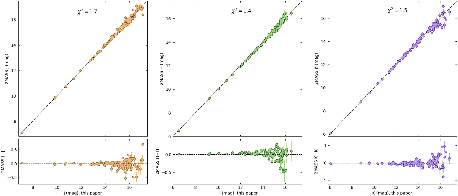
Figure 13: One-to-one plots of recovered J, H and K magnitudes for brown dwarfs using SpeX spectra.

Appendix B Magnitude scaling

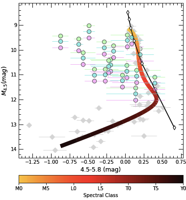
Figure 14: Colour-magnitude diagram with planetary magnitudes scaled by different factors: blue circles indicate scaling to a 0.9R_J object, pink circles indicate scaling to 0.8R_J, and green circles are planets scaled to a Jupiter sized object (R = R_J).

In figure 14 we present a colour-magnitude diagram where each planet has been scaled to a different size; this is to show the impact of choosing a different scaling factor. The size of the planets only affects their vertical positions, and small changes in the scale factors do not have a huge impact. In fact, provided all planets are scaled to the same size as each other, the main result is to entirely remove the effect of the differing planetary sizes. This in itself allows better comparison with brown dwarfs as they are considerably more homogeneous in size than planets.

Appendix C Tooklit Walkthrough

Users can interact with the ExoCMD_toolkit via our Jupyter applet . This makes the experience far easier as plot options can be selected via drop-down boxes and tick-boxes rather than having to write lines of code. In this section we will show how the applet works and some of the available options.

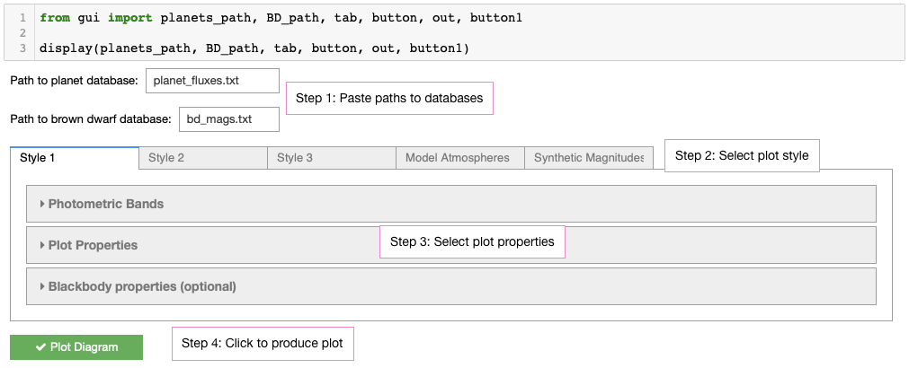
Figure 15: Applet view on first opening the Jupyter Notebook.

Figure 15 shows the applet as it appears on first opening the notebook. The code can be toggled on and off in order to see how the applet is interacting with the .py modules we have written. There are two boxes where users can paste the paths to the planet and brown dwarf databases after cloning the repository them from Github. These are prefilled, but can be edited if the names of the databases are changed. Once all selections for a particular style of plot have been made, users should click the ‘Plot diagram’ button. Diagrams will appear in the notebook and can be saved using the ‘Save figure’ button.

The ‘Style 1’ tab corresponds to the function ExoCMD_1, which produces colour-magnitude diagrams in the style of those presented in Triaud et al. (2014). ‘Style 2’ calls the function ExoCMD_2 and outputs plots in the same style as Figure 6. For the function ExoCMD_3, which allows users to highlight specific planets in a different colour as in Figures 3 and 4, users should select the ‘Style 3’ tab. Here it is necessary to enter the name of the host star placing a hyphen between letters and numbers. See Figure 16 for an example.

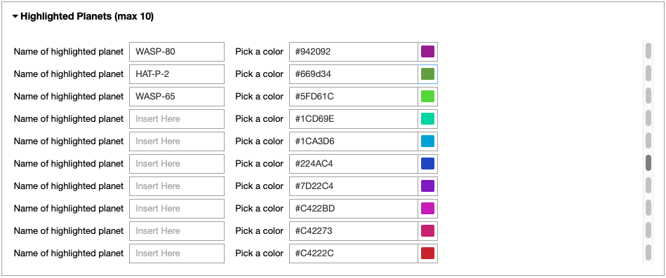
Figure 16: Selecting planets to highlight on a colour-magnitude diagram. The names are not case-sensitive but there must be hyphens between letters and numbers. Planet letters are omitted in this version.

The tab labelled ‘Model Atmospheres’ allows users to create colour-magnitude diagrams using the function ExoCMD_model in order to compare synthetic photometry with real planets. There are many options to choose from when setting the model spectra. Some defaults are always selected as constraining nothing will lead to photometry being computed for all 10,640 available spectra. While this can be done, it will be time consuming so users should only select ‘all’ for each parameter if that is what they wish to do. Figure 17 shows the layout of the accordion for this style of diagram.

Figure 17: ‘Style 3’ and ‘Model Atmospheres’ both have an extra element compared with ‘Style 1’ and ‘Style 2’. Here we show the view for ‘Model Atmospheres’ with a closed accordion.

The tab on the far right, labelled ‘Synthetic Magnitudes’, accesses a database of synthetic photometry derived from SpeX spectra. Plots produced will call the function ExoCMD_synth; available bands are 2MASS JHK, along with Sloan-z’, NB1190, NB2090 and W_JH.

With the exception of ‘Synthetic Magnitudes’, all four styles of plot have the same photometric bands available. They can also have a 0.9R_J blackbody added to the diagram, have a colourbar included or not, and can have planetary magnitudes adjusted to the size of a 0.9R_J object.

Appendix D Planet database

In these tables we present the planetary databases. Table LABEL:tab:composite contains eccentricities, radii, equilibrium temperatures, host star spectral types and astrometric distances to planets included in our database. Table LABEL:tab:fluxes contains secondary eclipse measurements in near- and mid-infrared bands for all planets we have included on our colour-magnitude diagrams. Both tables can be downloaded in .txt or .xlsx form from Githib.

Table 1: Composite planet data which we have in this paper. Compiled with the help of the NASA Exoplanet Archive.

Planet	Eccentricity	Radius (RJ)	Equilibrium Temperature (K)	Host Star Spectral Type	Distance (pc)	References
CoRoT-1 b	0	1.49$\pm$0.08	1898$\pm$50	G0 V	787.91$\pm$24.18	21 15
CoRoT-2 b	0.0143$\pm$0.0077	1.466${}^{+0.042}_{-0.044}$	1521$\pm$18	G7V	213.28$\pm$2.49	104 249 15 213
GJ 3470 b	0.017$\pm$0.016	0.408$\pm$0.016	594$\pm$97	M1.5	29.42$\pm$0.05	28 14 30 15
GJ 436 b	0.13827$\pm$0.00018	0.372$\pm$0.015	686$\pm$10	M2.5 V	9.75$\pm$0.01	160 273 47 15
HAT-P-1 b	0	1.319$\pm$0.019	1322${}^{+14}_{-15}$	G0 V	158.98$\pm$0.98	185 198 128 15
HAT-P-13 b	0.0133$\pm$0.0041	1.272$\pm$0.065	1740$\pm$27	G4	246.81$\pm$2.23	291 273 18 15
HAT-P-18 b	0.084$\pm$0.048	0.995$\pm$0.052	852$\pm$28	K2	161.4$\pm$0.61	112 15
HAT-P-19 b	0.067$\pm$0.042	1.132$\pm$0.072	1010$\pm$42	K1	202.08$\pm$1.47	112 15
HAT-P-2 b	0.5172$\pm$0.0019	0.951${}^{+0.039}_{-0.053}$	1540$\pm$30	F8	127.77$\pm$0.43	185 149 205 15
HAT-P-20 b	0.015$\pm$0.005	0.867$\pm$0.033	970$\pm$23	K3	71.04$\pm$0.2	19 15
HAT-P-23 b	0.11$\pm$0.04	1.09$\pm$0.23	1951$\pm$30	G0	364.81$\pm$4.77	253 59 19 15
HAT-P-3 b	0	0.94$\pm$0.07	1189$\pm$16	K	134.55$\pm$0.48	253 249 265 15
HAT-P-30 b	0.04$\pm$0.02	1.44$\pm$0.15	1630$\pm$42	F7	213.99$\pm$2.22	253 130 154 15
HAT-P-32 b	0.159${}^{+0.051}_{-0.028}$	1.98$\pm$0.045	1836$\pm$7	-	289.21$\pm$5.35	284 15
HAT-P-33 b	0	1.85$\pm$0.49	1782$\pm$28	F4	396.11$\pm$7.65	253 113 154 15
HAT-P-4 b	0	1.274${}^{+0.049}_{-0.06}$	1686${}^{+30}_{-26}$	G1 V	320.45$\pm$2.85	266 139 15
HAT-P-40 b	0	1.52$\pm$0.17	1770$\pm$33	F	464.47$\pm$6.54	253 114 15
HAT-P-41 b	0	2.05$\pm$0.5	1941$\pm$38	F	348.18$\pm$4.53	253 114 15
HAT-P-6 b	0	1.48$\pm$0.15	1675${}^{+32}_{-31}$	F8 V	275.36$\pm$3.64	253 266 15 93
HAT-P-7 b	0	1.51$\pm$0.21	2733$\pm$21	F6 V	341.08$\pm$2.43	253 193 15 93
HAT-P-8 b	0	1.4$\pm$0.13	1700$\pm$35	F6	211.55$\pm$1.71	253 144 154 15
HD 149026 b	0	0.74$\pm$0.02	1626${}^{+69}_{-37}$	G0	75.86$\pm$0.17	253 247 49 15
HD 189733 b	0	1.13$\pm$0.01	1209$\pm$11	K2 V	19.76$\pm$0.01	253 2 108 15
HD 209458 b	0	1.39$\pm$0.02	1459$\pm$12	F8	48.3$\pm$0.12	253 247 49 15
KELT-1 b	0.0099${}^{+0.01}_{-0.0069}$	1.11${}^{+0.032}_{-0.022}$	-	F5	268.43$\pm$3.06	238 15
KELT-2 A b	0	1.35$\pm$0.08	-	F8	134.06$\pm$0.8	253 49 15
KELT-3 b	0	1.56$\pm$0.11	1816${}^{+37}_{-39}$	F	210.25$\pm$5.54	253 208 15
KELT-7 b	0	1.6$\pm$0.06	2048$\pm$27	F	136.68$\pm$0.94	253 29 15
Kepler-13A b	$0.00064\begin{subarray}{c}+0.00012\\ -0.00016\end{subarray}$	1.512$\pm$0.035	2550$\pm$80	A	519.1$\pm$30.7	89 15 232
Kepler-5 b	0.043	1.426${}^{+0.036}_{-0.051}$	1750$\pm$20	F5V	899.78$\pm$16.77	31 89 15 97
Kepler-6 b	0.06	1.304${}^{+0.018}_{-0.033}$	1460$\pm$10	-	587.04$\pm$5.07	31 89 15
Qatar-1 b	0	1.143${}^{+0.026}_{-0.025}$	1418${}^{+28}_{-27}$	K	185.62$\pm$0.8	62 15 7
TrES-1 b	0	1.13$\pm$0.06	1140${}^{+13}_{-12}$	K0 V	159.66$\pm$0.74	253 266 5 15
TrES-2 b	0	1.36$\pm$0.08	1466$\pm$9	G0 V	215.32$\pm$1.05	253 204 199 15
TrES-3 b	0	1.336${}^{+0.031}_{-0.037}$	1638$\pm$22	G4 V	231.34$\pm$1.3	252 248 200 15
TrES-4 b	0	1.61$\pm$0.18	1778$\pm$22	F8 V	515.98$\pm$7.03	253 273 172 15
WASP-1 b	0	1.483${}^{+0.024}_{-0.034}$	1812$\pm$14	F7 V	393.07$\pm$10.8	159 273 61 15
WASP-10 b	0.0473${}^{+0.0034}_{-0.0029}$	1.08$\pm$0.02	1370$\pm$50	K5 V	141$\pm$0.75	138 129 226 15
WASP-100 b	0	1.33$\pm$0.14	2190$\pm$140	F2	364.41$\pm$2.75	253 119 15
WASP-101 b	0	1.43$\pm$0.09	1560$\pm$35	F6	201.22$\pm$1.15	253 119 15
WASP-103 b	0.15	1.528${}^{+0.073}_{-0.047}$	2508${}^{+75}_{-70}$	F8 V	883.3$\pm$120.5	31 106 15
WASP-104 b	0	1.137$\pm$0.037	1516$\pm$39	G8	185.93$\pm$1.48	244 15
WASP-12 b	0.0447	1.937$\pm$0.056	2593$\pm$57	G0 V	427.25$\pm$6.07	273 52 15
WASP-121 b	0	1.865$\pm$0.044	2358$\pm$52	F6 V	269.9$\pm$1.58	75 15
WASP-131 b	0	1.22$\pm$0.05	1460$\pm$30	G0	200.08$\pm$2.66	121 15
WASP-14 b	0.09	1.38$\pm$0.08	1872$\pm$29	F5V	162$\pm$0.81	253 215 15 87
WASP-17 b	0	1.87$\pm$0.24	1755$\pm$28	F4	405.91$\pm$8.78	253 250 269 15
WASP-18 b	0	1.191$\pm$0.038	2413$\pm$44	F6 IV	123.48$\pm$0.37	253 233 125 15
WASP-19 b	0.002${}^{+0.014}_{-0.002}$	1.392$\pm$0.04	2520	G8 V	268.33$\pm$1.72	293 116 15
WASP-2 b	0.0054${}^{+0.009}_{-0.0044}$	1.081${}^{+0.041}_{-0.04}$	1311${}^{+52}_{-50}$	K1 V	153.24$\pm$1.64	138 2 61 15
WASP-24 b	0	1.38$\pm$0.16	1772$\pm$29	F8/9	322.11$\pm$4.5	253 251 15 87
WASP-26 b	0	1.21$\pm$0.15	1650$\pm$24	G0	252.76$\pm$4.76	253 251 15 87
WASP-3 b	0	1.42$\pm$0.17	2020$\pm$35	F7 V	231.16$\pm$1.65	253 248 15 211
WASP-33 b	0	1.593$\pm$0.074	2782$\pm$41	A5	121.94$\pm$1	253 52 49 15
WASP-36 b	0.019	1.327$\pm$0.021	1733$\pm$19	G2	386.35$\pm$5.26	31 170 15 242
WASP-39 b	0	1.27$\pm$0.04	1166$\pm$14	G	213.98$\pm$1.76	92 171 15 278
WASP-4 b	0	1.321$\pm$0.039	1673$\pm$17	G7 V	267.21$\pm$3.77	32 249 289 15
WASP-43 b	0	0.93${}^{+0.07}_{-0.09}$	1427$\pm$9	K7 V	86.75$\pm$0.33	117 88 226 15
WASP-46 b	0.022	1.174$\pm$0.037	1636$\pm$44	G6 V	375.31$\pm$4.46	31 60 60 15
WASP-48 b	0	1.5$\pm$0.2	2035$\pm$52	G	454.14$\pm$4.47	253 273 15
WASP-5 b	0.038${}^{+0.026}_{-0.018}$	1.087${}^{+0.068}_{-0.071}$	1706${}^{+52}_{-48}$	G4 V	309.14$\pm$3.41	103 8 15
WASP-6 b	0.05	1.03$\pm$0.1	1184$\pm$16	G8 V	197.12$\pm$1.63	253 267 15
WASP-62 b	0	1.32$\pm$0.08	1475${}^{+25}_{-20}$	F7	175.63$\pm$0.59	253 34 15 118
WASP-63 b	0	1.41$\pm$0.14	-	G8	290.68$\pm$2.03	253 15 118
WASP-64 b	0	1.271$\pm$0.039	1689$\pm$49	G7	369.93$\pm$3.03	105 15
WASP-65 b	0	1.112$\pm$0.059	1480$\pm$10	G6	273.7$\pm$2.73	107 15
WASP-67 b	0	1.15$\pm$0.11	1003$\pm$20	K0 V	189.47$\pm$1.56	253 169 15 118
WASP-69 b	0	1.11$\pm$0.04	963$\pm$18	K5	49.96$\pm$0.13	253 50 12 15
WASP-74 b	0	1.36$\pm$0.1	1910$\pm$40	F9	149.22$\pm$1.15	253 120 15
WASP-76 b	0	1.83${}^{+0.06}_{-0.04}$	2160$\pm$40	F7	194.46$\pm$6.21	287 15
WASP-77 A b	0	1.38$\pm$0.09	1674$\pm$24	G8 V	105.17$\pm$1.21	253 273 178 15
WASP-78 b	0	1.93$\pm$0.45	2470${}^{+54}_{-56}$	F8	754.26$\pm$17.1	253 34 15 240
WASP-79 b	0	1.67$\pm$0.15	1716${}^{+26}_{-24}$	F5	246.69$\pm$1.82	253 34 15 240
WASP-8 b	0.31	1.13$\pm$0.05	-	G8 V	89.96$\pm$0.36	253 226 15
WASP-80 b	0.002${}^{+0.01}_{-0.002}$	0.999${}^{+0.03}_{-0.031}$	825$\pm$19	K7 V	49.79$\pm$0.12	272 270 15
WASP-87 b	0	1.385$\pm$0.06	-	F5	298.39$\pm$3.62	1 15 11
WASP-94 A b	0	1.58$\pm$0.13	1604${}^{+25}_{-22}$	F8	211.21$\pm$2.51	253 197 15
WASP-97 b	0	1.14$\pm$0.06	1555$\pm$40	G5	151.07$\pm$0.51	253 119 15
XO-1 b	0	1.14$\pm$0.07	1210$\pm$16	G1 V	163.55$\pm$0.62	253 247 180 15
XO-2 N b	0.028${}^{+0.038}_{-0.022}$	0.993$\pm$0.012	1328${}^{+17}_{-28}$	K0 V	154.27$\pm$1.46	138 68 249 46 15
XO-3 b	0.29	1.41$\pm$0.12	1729$\pm$34	F5 V	213.05$\pm$2.72	253 247 127 15
XO-4 b	0	1.25$\pm$0.08	1630${}^{+169}_{-36}$	F5 V	272.65$\pm$2.91	253 247 181 15

Table 2: Planet secondary eclipse measurements in near- and mid-infrared bands, including our W_JH band and H_s.

Planet	J	H	K	3.6$\mu$m	4.5$\mu$m	5.8$\mu$m	8.0$\mu$m	WJH	Hs	References
CoRoT-1 b	-	0.145$\pm$0.049	0.336$\pm$0.042	0.415$\pm$0.042	0.482$\pm$0.042	-	-	-	-	297 221 77
CoRoT-2 b	-	-	0.16$\pm$0.09	0.355$\pm$0.02	0.5$\pm$0.02	-	0.51$\pm$0.059	-	-	6 77
GJ 3470 b	-	-	-	0.0115${}^{+0.0027}_{0.0026}$	0.0003$\pm$0.0022	-	-	-	-	27
GJ 436 b	-	-	-	0.041$\pm$0.003	-	0.033$\pm$0.014	0.054$\pm$0.008	-	-	255
HAT-P-1 b	-	-	0.109$\pm$0.025	0.08$\pm$0.008	0.135$\pm$0.022	0.203$\pm$0.031	0.238$\pm$0.04	-	-	301 262
HAT-P-13 b	-	-	-	0.0801$\pm$0.0081	0.19$\pm$0.0124	-	-	-	-	111 102
HAT-P-18 b	-	-	-	0.0437${}^{+0.0146}_{-0.0144}$	0.0326${}^{+0.0144}_{-0.0147}$	-	-	-	-	280
HAT-P-19 b	-	-	-	0.062$\pm$0.014	0.062$\pm$0.016	-	-	-	-	133
HAT-P-2 b	-	-	-	0.0996$\pm$0.0072	0.1031$\pm$0.0061	0.071${}^{+0.029}_{-0.013}$	0.1392${}^{+0.0095}_{-0.0095}$	-	-	145
HAT-P-20 b	-	-	-	0.0615$\pm$0.0082	0.1096$\pm$0.0077	-	-	-	-	79
HAT-P-23 b	-	-	0.234$\pm$0.046	0.248$\pm$0.019	0.309$\pm$0.026	-	-	-	-	202 202
HAT-P-3 b	-	-	-	0.112${}^{+0.015}_{-0.03}$	0.094${}^{+0.016}_{-0.009}$	-	-	-	-	264
HAT-P-30 b	-	-	-	0.1584$\pm$0.0107	0.1825$\pm$0.0147	-	-	-	-	102
HAT-P-32 b	0.04$\pm$0.014	0.09$\pm$0.033	0.178$\pm$0.057	0.364$\pm$0.016	0.438$\pm$0.02	-	-	0.051$\pm$0.013	0.057$\pm$0.013	this work 298
HAT-P-33 b	-	-	-	0.1603$\pm$0.0127	0.1835$\pm$0.0199	-	-	-	-	102
HAT-P-4 b	-	-	-	0.142${}^{+0.014}_{-0.016}$	0.122${}^{+0.012}_{-0.014}$	-	-	-	-	264
HAT-P-40 b	-	-	-	0.0988$\pm$0.0168	0.1057$\pm$0.0145	-	-	-	-	102
HAT-P-41 b	-	-	-	0.1829$\pm$0.0319	0.2278$\pm$0.0177	-	-	-	-	102
HAT-P-6 b	-	-	-	0.117$\pm$0.008	0.106$\pm$0.006	-	-	-	-	263
HAT-P-7 b	-	-	-	0.098$\pm$0.017	0.159$\pm$0.022	0.245$\pm$0.031	0.262$\pm$0.027	-	-	58
HAT-P-8 b	-	-	-	0.131${}^{+0.007}_{-0.01}$	0.111${}^{+0.008}_{-0.007}$	-	-	-	-	263
HD 149026 b	-	-	-	0.04$\pm$0.003	0.034$\pm$0.006	0.044$\pm$0.01	0.052$\pm$0.006	-	-	256
HD 189733 b	-	-	-	0.256$\pm$0.014	0.214$\pm$0.02	0.31$\pm$0.034	0.344${}^{+0.0036}_{-0.0036}$	-	-	54
HD 209458 b	0.091$\pm$0.018	-	-	0.106${}^{+0.007}_{-0.008}$	0.133$\pm$0.011	0.142${}^{+0.059}_{-0.058}$	0.215$\pm$0.012	0.073$\pm$0.018	0.147$\pm$0.018	this work 90
KELT-1 b	-	-	0.16${}^{+0.018}_{0.02}$	0.195$\pm$0.01	0.2$\pm$0.012	-	-	-	-	67 24
KELT-2 A b	-	-	-	0.0572${}^{+0.0045}_{-0.0046}$	0.0616${}^{+0.0044}_{-0.0045}$	-	-	-	-	210
KELT-3 b	-	-	-	0.1766$\pm$0.0097	0.1656$\pm$0.0104	-	-	-	-	102
KELT-7 b	-	-	-	0.1688$\pm$0.0046	0.1896$\pm$0.0057	-	-	-	-	102
Kepler-13 Ab	0.0724$\pm$0.0071	-	0.122$\pm$0.051	0.156$\pm$0.031	0.222$\pm$0.023	-	-	0.071$\pm$0.08	0.086$\pm$0.008	this work 232
Kepler-5 b	-	-	-	0.103$\pm$0.017	0.107$\pm$0.015	-	-	-	-	81
Kepler-6 b	-	-	-	0.069$\pm$0.027	0.151$\pm$0.019	-	-	-	-	81
Qatar-1 b	-	-	0.136$\pm$0.034	0.149$\pm$0.051	0.273$\pm$0.049	-	-	-	-	67 101
TrES-1 b	-	-	-	0.083$\pm$0.024	0.094$\pm$0.024	0.162$\pm$0.042	0.213$\pm$0.042	-	-	71
TrES-2 b	-	-	0.062${}^{+0.013}_{-0.011}$	0.127$\pm$0.021	0.23$\pm$0.024	0.199$\pm$0.054	0.359$\pm$0.06	-	-	64 201
TrES-3 b	-	-	0.133${}^{+0.018}_{-0.016}$	0.356$\pm$0.035	0.372$\pm$0.054	0.449$\pm$0.097	0.475$\pm$0.046	0.047$\pm$0.028	-	65 98
TrES-4 b	-	-	-	0.137$\pm$0.011	0.148$\pm$0.016	0.261$\pm$0.059	0.318$\pm$0.044	-	-	136
WASP-1 b	-	-	-	0.184$\pm$0.016	0.217$\pm$0.017	0.274$\pm$0.058	0.474$\pm$0.046	-	-	288
WASP-10 b	-	-	0.137${}^{+0.013}_{-0.019}$	0.1$\pm$0.011	0.146$\pm$0.016	-	-	-	-	69 133
WASP-100	-	-	-	0.1267$\pm$0.0098	0.172$\pm$0.0119	-	-	-	-	102
WASP-101	-	-	-	0.1161$\pm$0.0111	0.1194$\pm$0.0113	-	-	-	-	102
WASP-103 b	0.131$\pm$0.02	-	0.3567${}^{+0.04}_{-0.035}$	0.3702$\pm$0.0256	0.4711$\pm$0.0339	-	-	0.146$\pm$0.027	0.16$\pm$0.03	this work 76 102
WASP-104 b	-	-	-	0.1709$\pm$0.0195	0.2643$\pm$0.0303	-	-	-	-	102
WASP-12 b	0.139$\pm$0.03	0.176${}^{+0.016}_{-0.021}$	0.296$\pm$0.014	0.421$\pm$0.011	0.428$\pm$0.012	0.696$\pm$0.06	0.696$\pm$0.096	0.198$\pm$0.022	0.205$\pm$0.022	this work 66 67 258
WASP-121 b	0.107$\pm$0.011	-	-	0.367$\pm$0.013	0.4684$\pm$0.0121	-	-	0.125$\pm$0.011	0.13$\pm$0.11	this work 91 102
WASP-131 b	-	-	-	0.0364$\pm$0.0097	0.0282$\pm$0.0078	-	-	-	-	102
WASP-14 b	-	-	-	0.1816$\pm$0.0067	0.2284$\pm$0.009	-	0.181$\pm$0.022	-	-	102
WASP-17 b	-	-	-	-	0.229$\pm$0.013	-	0.237$\pm$0.039	-	-	9
WASP-18 b	0.094$\pm$0.004	-	0.13$\pm$0.03	0.2973$\pm$0.007	0.3858$\pm$0.0113	0.37$\pm$0.03	0.41$\pm$0.02	0.108$\pm$0.004	0.113$\pm$0.004	this work 300 231
WASP-19 b	-	0.276$\pm$0.044	0.287$\pm$0.02	0.483$\pm$0.025	0.572$\pm$0.03	0.65$\pm$0.11	0.73$\pm$0.12	-	-	10 299 10
WASP-2 b	-	-	-	0.083$\pm$0.035	0.169$\pm$0.017	0.192$\pm$0.077	0.285$\pm$0.059	-	-	288
WASP-24 b	-	-	-	0.159$\pm$0.013	0.202$\pm$0.018	-	-	-	-	243
WASP-26 b	-	-	-	0.126$\pm$0.013	0.149$\pm$0.016	-	-	-	-	168
WASP-3 b	-	-	0.193$\pm$0.014	0.209${}^{+0.04}_{-0.028}$	0.282$\pm$0.012	-	0.328${}^{+0.086}_{-0.055}$	-	-	67 222
WASP-33 b	0.11$\pm$0.03	-	0.244${}^{+0.027}_{-0.02}$	0.26$\pm$0.05	0.41$\pm$0.02	-	-	0.123$\pm$0.025	0.13$\pm$0.03	this work 302 78
WASP-36 b	-	-	0.13$\pm$0.04	-	-	-	-	-	-	300
WASP-39 b	-	-	-	0.088$\pm$0.015	0.096$\pm$0.018	-	-	-	-	133
WASP-4 b	-	-	0.185${}^{+0.014}_{-0.013}$	0.319$\pm$0.031	0.343$\pm$0.027	-	-	-	-	48 25
WASP-43 b	0.042$\pm$0.0045	0.103$\pm$0.017	0.194$\pm$0.029	0.3773$\pm$0.0138	0.3866$\pm$0.0195	-	-	0.036$\pm$0.004	0.056$\pm$0.004	this work 281 102
WASP-46 b	0.129$\pm$0.055	0.194$\pm$0.078	0.26${}^{+0.05}_{-0.03}$	0.136$\pm$0.0701	0.4446$\pm$0.0589	-	-	-	-	56 300 102
WASP-48 b	-	0.047$\pm$0.016	0.109$\pm$0.027	0.176$\pm$0.013	0.214$\pm$0.02	-	-	-	-	202 202
WASP-5 b	0.168${}^{+0.05}_{-0.052}$	-	0.2$\pm$0.02	0.197$\pm$0.028	0.237$\pm$0.024	-	-	-	-	55 300 22
WASP-6 b	-	-	-	0.094$\pm$0.019	0.115$\pm$0.022	-	-	-	-	133
WASP-62 b	-	-	-	0.1616$\pm$0.0146	0.1359$\pm$0.013	-	-	-	-	102
WASP-63 b	-	-	-	0.0522$\pm$0.0095	0.0533$\pm$0.0128	-	-	-	-	102
WASP-64 b	-	-	-	0.2859$\pm$0.027	0.2071$\pm$0.0471	-	-	-	-	102
WASP-65 b	-	-	-	0.1587$\pm$0.0245	0.0724$\pm$0.0318	-	-	-	-	102
WASP-67 b	-	-	-	0.022$\pm$0.013	0.08$\pm$0.018	-	-	-	-	133
WASP-69 b	-	-	-	0.0421$\pm$0.0029	0.0463$\pm$0.0039	-	-	-	-	280
WASP-74 b	-	-	-	0.1446$\pm$0.0066	0.2075$\pm$0.01	-	-	-	-	102
WASP-76 b	-	-	-	0.2645$\pm$0.0063	0.3345$\pm$0.0082	-	-	-	-	102
WASP-77 b	-	-	-	0.1845$\pm$0.0094	0.2362$\pm$0.0127	-	-	-	-	102
WASP-78 b	-	-	-	0.2001$\pm$0.0218	0.2013$\pm$0.0351	-	-	-	-	102
WASP-79 b	-	-	-	0.1394$\pm$0.0088	0.1783$\pm$0.0106	-	-	-	-	102
WASP-8 b	-	-	-	0.113$\pm$0.018	0.0692$\pm$0.0068	-	0.093$\pm$0.023	-	-	70
WASP-80 b	-	-	-	0.455$\pm$0.1	0.944$\pm$0.064	-	-	-	-	272
WASP-87 b	-	-	-	0.2077$\pm$0.0127	0.2705$\pm$0.0137	-	-	-	-	102
WASP-94A b	-	-	-	0.0867$\pm$0.0059	0.0995$\pm$0.0093	-	-	-	-	102
WASP-97 b	-	-	-	0.1359$\pm$0.0084	0.1534$\pm$0.0101	-	-	-	-	102
XO-1 b	-	-	-	0.086$\pm$0.007	0.122$\pm$0.009	0.261$\pm$0.031	0.21$\pm$0.029	-	-	156
XO-2 N b	-	-	-	0.081$\pm$0.017	0.098$\pm$0.02	0.167$\pm$0.036	0.133$\pm$0.049	-	-	157
XO-3 b	-	-	-	0.101$\pm$0.004	0.158$\pm$0.0036	0.134$\pm$0.049	0.15$\pm$0.036	-	-	158 292
XO-4 b	-	-	-	0.056${}^{+0.012}_{-0.006}$	0.135$\pm$0.01	-	-	-	-	263

Appendix E Updated Plots

In this section we present updated versions of all near- and mid-infrared plots presented in Triaud et al. (2014)

In Figure 18 we present updated colour-magnitude diagrams in the 2MASS photometric bands, J, H and K. The absolute magnitudes of planets have been scaled to a $\rm 0.9R_{J}$ object coincide with the typical size of a brown dwarf. Additionally, we have plotted the location of a $\rm 0.9R_{J}$ blackbody at temperatures of 1500K, 2500K, 3500K and 4500K. The mean position of the brown dwarf sequence is shown by a polynomial coloured by spectral type, computed using coefficients provided by Dupuy & Liu (2012). Due to the low number of J-band fluxes measured for exoplanets, we have supplemented the data with our photometry computed from HST/WFC3 low resolution spectra.

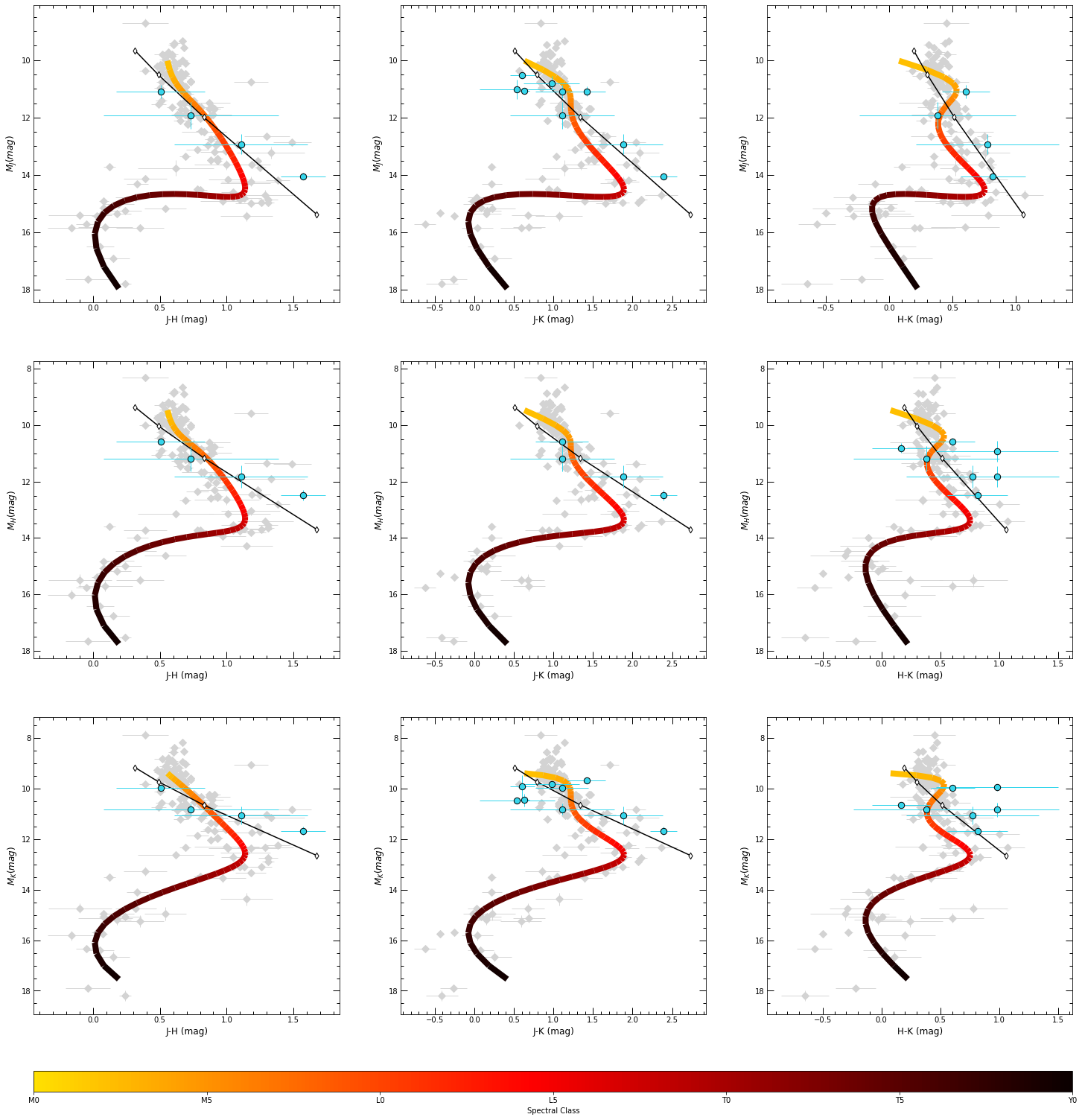
Figure 18: Updated near-infrared colour-magnitude diagrams in near-infrared photometric bands, similar to those first published in Triaud et al. (2014), plotted using our ExoCMD_2 plotting function. Magnitudes have been adjusted to coincide with an object of radius $\rm 0.9R_{J}$ for easier comparison with brown dwarfs. We have also plotted in black the location of a $\rm 0.9R_{J}$ blackbody as a black line; the white-filled diamonds show the position of the blackbody at temperatures of 1500K, 2500K, 3500K and 4500K. The polynomial representing the mean sequence of the brown dwarfs has been coloured according to spectral type.

The small number of planets presented in Triaud et al. (2014) appeared to be equally compatible with the ultra-cool dwarfs and the blackbody sequence. This remains the case, which is in agreements also with the near-infrared colour-magnitude diagrams presented recently in Manjavacas et al. (2019). Parmentier et al. (2018) writes that objects belonging to the subclass of ultra-hot Jupiters should lack any emission and absorption features, instead resembling a blackbody. At this time is is still impossible to disentangle which family of objects the planets resemble most; all objects which appear excessively blue or red have errors which make interpretations ambiguous. However, in Section 3.4 we see that in our newly created mid-infrared, the $W_{JH}$-band, we begin to see a departure from both the blackbody sequence and the narrow spread in colour of the M and L brown dwarfs.

In Figure 19 we present three near-infrared colour-magnitude diagrams produced using ExoCMD_synth using H_s) photometry instead of 2MASS H. These plots represent the rising diagonal in Figure 18 and we are able to showcase the positions of several more planets which have low resolution spectra measured with HST’s WFC3 instrument.

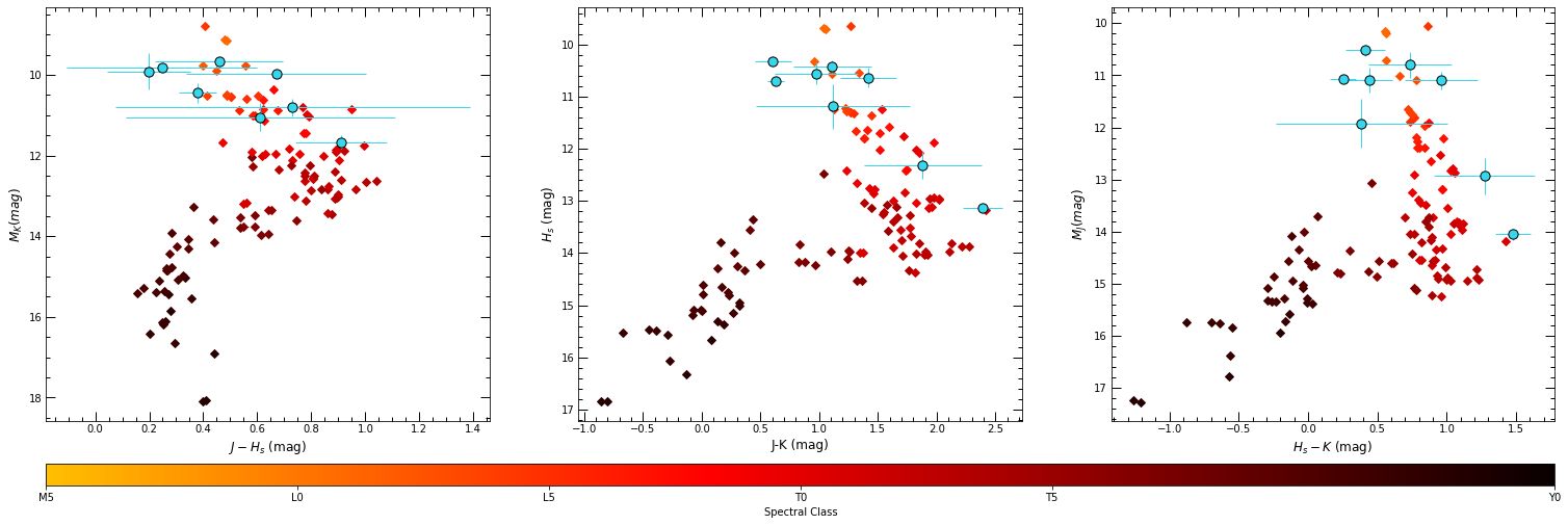
Figure 19: Near-infrared colour-magnitude diagrams plotted using our ExoCMD_synth. Planets are shown as blue circles in the foreground, whereas ultra-cool dwarfs are plotted as diamonds in the background coloured according to spectral type. This is similar to Fig. 18, but here using the H_s band instead.

In Figure 20 we present updated colour-magnitudes in Spitzer’s mid-infrared channels 1-4. Absolute magnitudes have once again been scaled to facilitate comparison with brown dwarfs. In black we show the blackbody sequence, with the unfilled diamonds indicating the position of a $\rm 0.9R_{J}$ blackbody of temperature 750K, 1750K, 2750K, 3750K and 4750K. We continue to plot the mean sequence of brown dwarfs using polynomial coefficients as above.

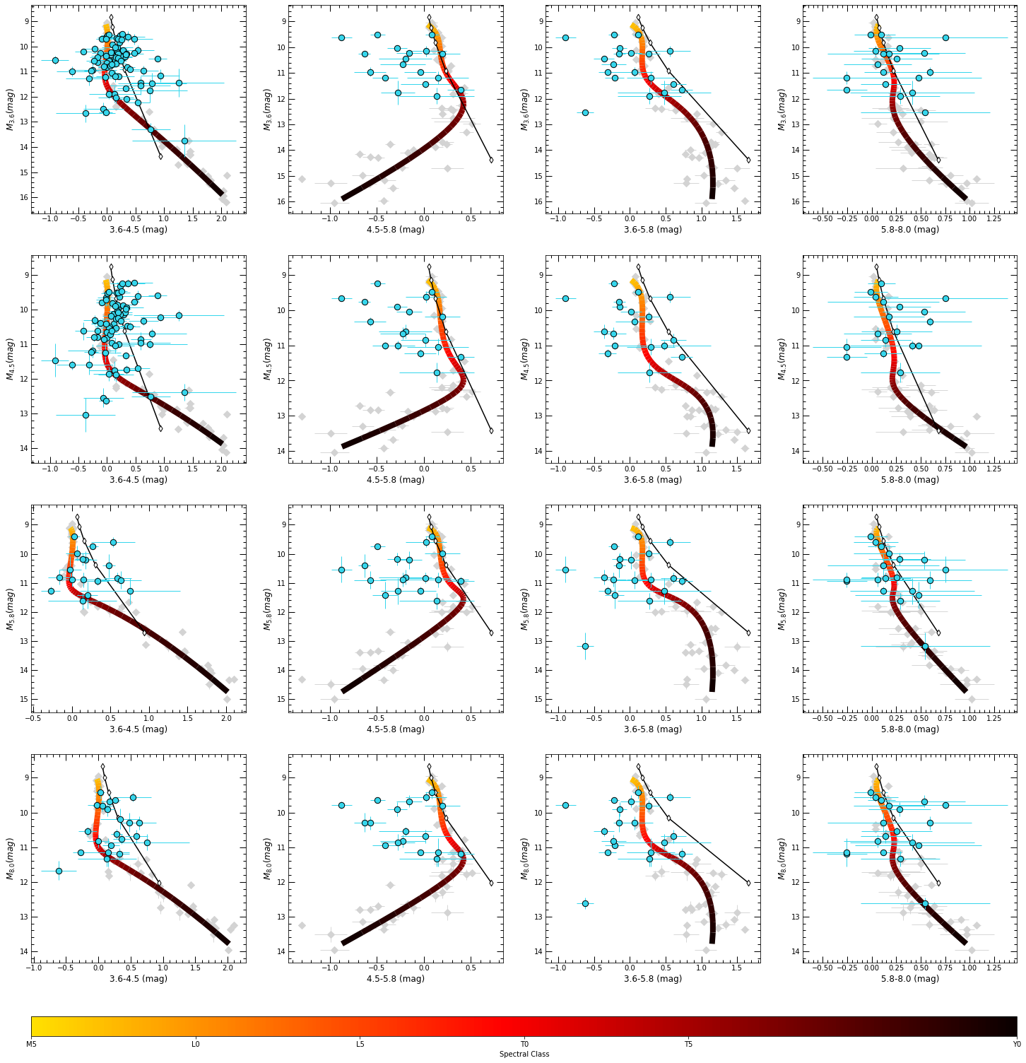
Figure 20: Updated near-infrared colour-magnitude diagrams in mid-infrared photometric bands, similar to those first published in Triaud et al. (2014), plotted using our ExoCMD_2 plotting function. Magnitudes have been adjusted to coincide with an object of radius $\rm 0.9R_{J}$ for more straight-forward comparison with the brown dwarf sequence. As before, we have also plotted a $0.9\rm R_{J}$ blackbody with a black line, highlighting temperatures of 750K, 1750K, 2750K, 3750K and 4750K. The polynomial representing the mean sequence of the brown dwarfs has been coloured according to spectral type.

The biggest increase in measurements can be seen in the top two plots on the far left, principally due to the contribution from Garhart et al. (2019). There is some increased scatter evident in these plots, and in $M_{4.5}$ vs [3.6$\mu$m - 4.5$\mu$m] in particular we are beginning to see an emerging sub-population of cooler objects which depart from both the brown dwarfs and the blackbodies. We explore this further in Section 3.2.

Appendix F Brown Dwarf Photometry

Here we present a summary of the photometry we computed from SpeX spectra for this paper, along with astrometric distances derived from parallaxes found in Dupuy & Liu (2012).

Table 3: Photometry computed from SpeX spectra using our Synth.ph module.

Name	Distance (pc)	Apparent magnitudes (mag)								Refs
		mJ	mH	mK	m${}_{W_{JH}}$	m${}_{H_{s}}$	mNB1190	mNB2090	m${}_{z^{\prime}}$
2MASP J0345432+254023	26.95$\pm$0.36	13.96$\pm$0	13.23$\pm$0	12.69$\pm$0	13.89$\pm$0	13.46$\pm$0	14.14$\pm$0	12.84$\pm$0	16.02$\pm$0	36, 74
2MASS J00345157+0523050	38.3$\pm$2.76	15.12$\pm$0	14.23$\pm$0	13.52$\pm$0	15.16$\pm$0	14.5$\pm$0	15.4$\pm$0	13.7$\pm$0	17.58$\pm$0	37, 148
2MASS J00501994-3322402	10.68$\pm$0.41	15.42$\pm$0	15.2$\pm$0	15.1$\pm$0	17.4$\pm$0.01	15.1$\pm$0	16.45$\pm$0	14.51$\pm$0	18.6$\pm$0	39, 276
2MASS J02572581-3105523	30.18$\pm$3.83	16.61$\pm$0	15.56$\pm$0	14.98$\pm$0	16.93$\pm$0.01	15.8$\pm$0	17.01$\pm$0.01	14.97$\pm$0	18.97$\pm$0.01	234, 276
2MASS J04070752+1546457	5.71$\pm$0.06	15.55$\pm$0	15.38$\pm$0	15.68$\pm$0	18.34$\pm$0	15.11$\pm$0	17.2$\pm$0	14.92$\pm$0	18.88$\pm$0	42, 84
2MASS J05160945-0445499	9.06$\pm$0.33	14.42$\pm$0	13.43$\pm$0	12.79$\pm$0	14.62$\pm$0	13.68$\pm$0	14.79$\pm$0.01	12.85$\pm$0	16.66$\pm$0	42, 94
2MASS J06244595-4521548	8.7$\pm$0.3	13.49$\pm$0	12.43$\pm$0	11.67$\pm$0	13.59$\pm$0	12.74$\pm$0	13.74$\pm$0	11.79$\pm$0	15.97$\pm$0	234, 95
2MASS J09393548-2448279	8.89$\pm$0.07	15.68$\pm$0	15.61$\pm$0	15.61$\pm$0	18.54$\pm$0.02	15.4$\pm$0	17.02$\pm$0.01	14.9$\pm$0	19.04$\pm$0	38, 84
2MASS J09490860-1545485	16.96$\pm$0.28	13.53$\pm$0	12.66$\pm$0	12.01$\pm$0	13.38$\pm$0	14.11$\pm$0	13.77$\pm$0.01	12.15$\pm$0	15.74$\pm$0	38, 82
2MASS J10073369-4555147	16.72$\pm$2.27	15.44$\pm$0	14.4$\pm$0	13.67$\pm$0	15.42$\pm$0	12.85$\pm$0	15.84$\pm$0	13.77$\pm$0	17.78$\pm$0	150, 94
2MASS J11061197+2754225	10.56$\pm$0.42	15.94$\pm$0	15.82$\pm$0	16.23$\pm$0	18.33$\pm$0.01	14.47$\pm$0	16.98$\pm$0.01	15.65$\pm$0.01	19.11$\pm$0	150, 276
2MASS J11263991-5003550	11.01$\pm$0.27	15.93$\pm$0	15.81$\pm$0.01	15.74$\pm$0.01	18.11$\pm$0.02	14.63$\pm$0	17.36$\pm$0.03	15.02$\pm$0.01	19.58$\pm$0	41, 261
2MASS J12373919+6526148	30.2$\pm$4.39	16.73$\pm$0	15.74$\pm$0.01	15.04$\pm$0	16.97$\pm$0.01	15.68$\pm$0	17.26$\pm$0.02	15.12$\pm$0.01	19.08$\pm$0.01	146, 276
2MASS J13313310+3407583	12.94$\pm$0.25	12.95$\pm$0	12.15$\pm$0	11.56$\pm$0	12.96$\pm$0	15.57$\pm$0.01	13.31$\pm$0	11.7$\pm$0	15.09$\pm$0	135, 282
2MASS J15200224-4422419A	12.94$\pm$0.25	12.95$\pm$0	12.15$\pm$0	11.57$\pm$0	12.97$\pm$0	15.96$\pm$0.01	13.15$\pm$0	11.71$\pm$0	15.1$\pm$0	40, 282
2MASS J15200224-4422419B	17.49$\pm$0.28	13.86$\pm$0	12.98$\pm$0	12.35$\pm$0	13.84$\pm$0	12.36$\pm$0	14.08$\pm$0.01	12.49$\pm$0.01	16.06$\pm$0	40, 286
2MASS J15462718-3325111	14.08$\pm$0.6	15.39$\pm$0	14.88$\pm$0	14.9$\pm$0	16.72$\pm$0	13.23$\pm$0	16.08$\pm$0	14.52$\pm$0	18.46$\pm$0	42, 173
2MASS J16150413+1340079	14.5$\pm$0.72	15.88$\pm$0	15.69$\pm$0	15.65$\pm$0	17.72$\pm$0.01	14.95$\pm$0	16.79$\pm$0.01	15.06$\pm$0	18.95$\pm$0	150, 276
2MASS J17502484-0016151	9.49$\pm$0.68	15.63$\pm$0	15.54$\pm$0	16.02$\pm$0	18.02$\pm$0.01	15.61$\pm$0	17.02$\pm$0	15.42$\pm$0	18.85$\pm$0	44, 94
2MASS J18212815+1414010	10.57$\pm$0.27	15.7$\pm$0	15.65$\pm$0	15.57$\pm$0.01	18.01$\pm$0.02	15.38$\pm$0	17.16$\pm$0.02	14.81$\pm$0.01	19.07$\pm$0	152, 84
2MASS J18283572-4849046	10.03$\pm$0.67	14.68$\pm$0	13.55$\pm$0	12.83$\pm$0	14.7$\pm$0	15.43$\pm$0.01	15.11$\pm$0	12.87$\pm$0	16.96$\pm$0	37, 176
2MASS J21392676+0220226	34.58$\pm$1.49	15.52$\pm$0.01	14.33$\pm$0.01	13.55$\pm$0.01	15.36$\pm$0.01	13.82$\pm$0	15.96$\pm$0.02	13.69$\pm$0.03	18.18$\pm$0.01	38, 148
2MASS J21403907+3655563	12.31$\pm$0.07	14.49$\pm$0	13.35$\pm$0	12.57$\pm$0	14.46$\pm$0	14.57$\pm$0.01	14.76$\pm$0	12.66$\pm$0	16.98$\pm$0	135, 286
2MASS J21481633+4003594	5.34$\pm$0.13	15.87$\pm$0.01	15.7$\pm$0.01	16.73$\pm$0.01	18.59$\pm$0.03	15.55$\pm$0	17.36$\pm$0.02	16.07$\pm$0.04	19.11$\pm$0.01	135, 43
2MASS J21513839-4853542	5.34$\pm$0.13	15.9$\pm$0	15.72$\pm$0	16.7$\pm$0.01	18.5$\pm$0.02	13.59$\pm$0	17.31$\pm$0.02	16.17$\pm$0.02	18.89$\pm$0	38, 43
2MASS J21542494-1023022	18.08$\pm$2.16	16.07$\pm$0	15.32$\pm$0	15.24$\pm$0	16.87$\pm$0.01	15.49$\pm$0	16.45$\pm$0.01	14.99$\pm$0.01	18.99$\pm$0	150, 94
2MASS J22282889-4310262	18.08$\pm$2.16	16.09$\pm$0	15.32$\pm$0	15.22$\pm$0	16.78$\pm$0	15.45$\pm$0	16.52$\pm$0	14.94$\pm$0	18.99$\pm$0	37, 94
2MASS J22425317+2542573	14.08$\pm$1.03	15.76$\pm$0	15.6$\pm$0.01	15.53$\pm$0.01	17.58$\pm$0.02	15.49$\pm$0.01	16.76$\pm$0.02	14.91$\pm$0.02	18.81$\pm$0.01	44, 94
2MASS J23512200+3010540	16.84$\pm$0.47	14.03$\pm$0	13.29$\pm$0	12.79$\pm$0	14.43$\pm$0	14.26$\pm$0	14.29$\pm$0	12.9$\pm$0.01	16.36$\pm$0	135, 82
2MASSI J0117474-340325	10.41$\pm$0.52	15.82$\pm$0	15.73$\pm$0	16.26$\pm$0.01	18.18$\pm$0.01	13.56$\pm$0	17.07$\pm$0.01	15.73$\pm$0.01	19.03$\pm$0	42, 276
2MASSI J0243137-245329	28.11$\pm$1.23	14.21$\pm$0	13.39$\pm$0	12.76$\pm$0	14.01$\pm$0	15.57$\pm$0	14.39$\pm$0	12.92$\pm$0	16.35$\pm$0	37, 148
2MASSI J0328426+230205	18.52$\pm$0.04	13.6$\pm$0	12.76$\pm$0	12.19$\pm$0	13.59$\pm$0	13.6$\pm$0	13.87$\pm$0	12.33$\pm$0	16.01$\pm$0	42, 224
2MASSI J0415195-093506	18.52$\pm$0.04	14.58$\pm$0	13.78$\pm$0	13.25$\pm$0	14.75$\pm$0	12.97$\pm$0	14.83$\pm$0	13.35$\pm$0	16.54$\pm$0	37, 224
2MASSI J0439010-235308	11.36$\pm$0.25	15.57$\pm$0	15.43$\pm$0	15.56$\pm$0.01	17.64$\pm$0.01	14$\pm$0	16.51$\pm$0.01	15.01$\pm$0.01	18.68$\pm$0	35, 261
2MASSI J0652307+471034	14.58$\pm$1.36	16.16$\pm$0	16.16$\pm$0.01	16.24$\pm$0.01	18.24$\pm$0.02	15.39$\pm$0	17.15$\pm$0.02	15.64$\pm$0.01	19.2$\pm$0.01	44, 94
2MASSI J0727182+171001	9.22$\pm$0.22	13.3$\pm$0	12.41$\pm$0	11.84$\pm$0	13.63$\pm$0	16.01$\pm$0.01	13.69$\pm$0	11.93$\pm$0	15.52$\pm$0	39, 13
2MASSI J0825196+211552	9.38$\pm$0.02	13.4$\pm$0	12.39$\pm$0	11.68$\pm$0	13.57$\pm$0	12.69$\pm$0	13.8$\pm$0	11.83$\pm$0	15.78$\pm$0	44, 225
2MASSI J0847287-153237	11.38$\pm$0.26	15.21$\pm$0	15$\pm$0	15.04$\pm$0	17.17$\pm$0	12.69$\pm$0	16.17$\pm$0.01	14.53$\pm$0.01	18.27$\pm$0	183, 241
2MASSI J0937347+293142	9.85$\pm$0.19	15.05$\pm$0.01	14.19$\pm$0.01	13.74$\pm$0.01	15.9$\pm$0.01	14.93$\pm$0	15.66$\pm$0.04	13.66$\pm$0.03	17.96$\pm$0	39, 241
2MASSI J1010148-040649	9.85$\pm$0.19	15.09$\pm$0	14.17$\pm$0	13.72$\pm$0	15.93$\pm$0	14.5$\pm$0.02	15.52$\pm$0	13.63$\pm$0	17.95$\pm$0	219, 241
2MASSI J1047538+212423	87.49$\pm$7.65	15.8$\pm$0	15.05$\pm$0	14.47$\pm$0	15.7$\pm$0.01	15.24$\pm$0.01	15.97$\pm$0.01	14.62$\pm$0.01	17.38$\pm$0.01	42, 148
2MASSI J1217110-031113	9.9$\pm$0.17	14.15$\pm$0	12.81$\pm$0	11.73$\pm$0	14.07$\pm$0	13.16$\pm$0	14.64$\pm$0	11.9$\pm$0	16.88$\pm$0	39, 148
2MASSI J1711457+223204	16.67$\pm$1.06	15.66$\pm$0	15.29$\pm$0	15.36$\pm$0	17.07$\pm$0.01	15.36$\pm$0	16.31$\pm$0	14.94$\pm$0	18.9$\pm$0	44, 241
2MASSI J1807159+501531	10.86$\pm$0.31	15.56$\pm$0	15.47$\pm$0	15.29$\pm$0	17.44$\pm$0	16.47$\pm$0	16.68$\pm$0.02	14.59$\pm$0.02	18.76$\pm$0	42, 241
2MASSI J2104149-103736	20.86$\pm$1.19	14.77$\pm$0	13.79$\pm$0	13.04$\pm$0.01	14.59$\pm$0.01	15.32$\pm$0.01	15.19$\pm$0.01	13.17$\pm$0.04	17.06$\pm$0.01	44, 282
2MASSI J2254188+312349	20.86$\pm$1.19	14.78$\pm$0	13.8$\pm$0	13.03$\pm$0	14.65$\pm$0	13.99$\pm$0	15.08$\pm$0	13.18$\pm$0	17.05$\pm$0	37, 282
2MASSI J2356547-155310	24.26$\pm$0.83	15.89$\pm$0	14.8$\pm$0	13.94$\pm$0	15.85$\pm$0	15.05$\pm$0	16.23$\pm$0	14.06$\pm$0	18.29$\pm$0	38, 148
2MASSs J0850359+105716	7.47$\pm$0.03	12.8$\pm$0	11.91$\pm$0	11.33$\pm$0	12.9$\pm$0	13.87$\pm$0	13.13$\pm$0.01	11.42$\pm$0.01	15.06$\pm$0	45, 286
2MASSW J1239272+551537	15.24$\pm$0.49	15.84$\pm$0	14.69$\pm$0	13.95$\pm$0	15.95$\pm$0.01	12.13$\pm$0.01	16.22$\pm$0.01	13.98$\pm$0.01	18.03$\pm$0	44, 74
2MASSW J1507476-162738	15.24$\pm$0.49	15.85$\pm$0	14.7$\pm$0	13.92$\pm$0	15.82$\pm$0	14.95$\pm$0	16.26$\pm$0	13.96$\pm$0.01	18.15$\pm$0	35, 74
2MASSW J1632291+190441	25.84$\pm$0.47	15.95$\pm$0	14.77$\pm$0	13.93$\pm$0	15.93$\pm$0	15.02$\pm$0	16.35$\pm$0.01	14.01$\pm$0	18.43$\pm$0.01	35, 84
2MASSW J1728114+394859	33.22$\pm$0.88	16.45$\pm$0	15.27$\pm$0	14.44$\pm$0	16.51$\pm$0.01	15.55$\pm$0.01	16.77$\pm$0.01	14.55$\pm$0.01	18.78$\pm$0.01	45, 84
DENIS J124514.1-442907	78.99$\pm$12.92	14.55$\pm$0	13.85$\pm$0	13.28$\pm$0	14.59$\pm$0	14.14$\pm$0	14.73$\pm$0	13.46$\pm$0.01	16.63$\pm$0	151, 285
GJ 1001B	12.98$\pm$0.35	13.09$\pm$0	12.09$\pm$0	11.37$\pm$0	13.12$\pm$0	12.33$\pm$0	13.41$\pm$0	11.5$\pm$0	15.54$\pm$0	35, 82
Gl 337CD	20.36$\pm$0.22	15.58$\pm$0	14.56$\pm$0	14.03$\pm$0	15.82$\pm$0	14.77$\pm$0.01	15.98$\pm$0	14.01$\pm$0	17.9$\pm$0	44, 303
Gl 584C	17.86$\pm$0.25	16.13$\pm$0	14.96$\pm$0	14.23$\pm$0	16.2$\pm$0.01	15.23$\pm$0	16.38$\pm$0.01	14.26$\pm$0.01	18.49$\pm$0.01	44, 303
Gliese 417BC	21.93$\pm$0.21	14.58$\pm$0	13.5$\pm$0	12.73$\pm$0	14.62$\pm$0	13.78$\pm$0	14.99$\pm$0	12.89$\pm$0	17.08$\pm$0	44, 303
Gliese 570D	5.84$\pm$0.03	15.2$\pm$0	15.12$\pm$0.01	15.47$\pm$0	18.13$\pm$0	14.91$\pm$0.01	16.79$\pm$0.02	14.73$\pm$0.01	18.39$\pm$0	37, 303
HD 89744B	39.43$\pm$0.48	14.86$\pm$0	14.1$\pm$0	13.56$\pm$0	14.8$\pm$0	14.3$\pm$0	15.19$\pm$0	13.73$\pm$0	16.92$\pm$0	42, 303
HN Peg	17.89$\pm$0.14	16.02$\pm$0	15.28$\pm$0	15.05$\pm$0	17.21$\pm$0	15.49$\pm$0	16.54$\pm$0	14.84$\pm$0	18.85$\pm$0	153, 303
LHS 2924	11.01$\pm$0.16	11.97$\pm$0	11.26$\pm$0	10.73$\pm$0	11.87$\pm$0	11.48$\pm$0	12.1$\pm$0	10.88$\pm$0	13.91$\pm$0	36, 190
LHS 3566	17.46$\pm$0.82	11.37$\pm$0	10.76$\pm$0	10.34$\pm$0	11.2$\pm$0	10.89$\pm$0	11.59$\pm$0	10.46$\pm$0	12.76$\pm$0	37, 63
LP 944-20	6.41$\pm$0.04	10.74$\pm$0	10.04$\pm$0	9.52$\pm$0	10.72$\pm$0	10.28$\pm$0	11.05$\pm$0	9.68$\pm$0	12.72$\pm$0	42, 82
SDSS J000013.54+255418.6	14.12$\pm$0.38	15.1$\pm$0	14.71$\pm$0	14.82$\pm$0	16.81$\pm$0	14.75$\pm$0	15.77$\pm$0	14.36$\pm$0	18.04$\pm$0	38, 84
SDSS J015141.69+124429.6	21.4$\pm$1.54	16.51$\pm$0	15.57$\pm$0	15.27$\pm$0	16.94$\pm$0.01	15.77$\pm$0	16.75$\pm$0	15.17$\pm$0	18.93$\pm$0	37, 276
SDSS J020742.48+000056.2	34.13$\pm$4.66	16.38$\pm$0.01	15.99$\pm$0.01	15.95$\pm$0.01	17.92$\pm$0.02	16.01$\pm$0.01	17$\pm$0.02	15.57$\pm$0.03	19.56$\pm$0.01	38, 175
SDSS J032553.17+042540.1	17.99$\pm$3.53	16.36$\pm$0	16.12$\pm$0	16.35$\pm$0	18.24$\pm$0	16.06$\pm$0	17.3$\pm$0.02	15.85$\pm$0	19.51$\pm$0	57, 94
SDSS J074201.41+205520.5	15.04$\pm$1.94	15.75$\pm$0	15.56$\pm$0	15.74$\pm$0	17.77$\pm$0.01	15.49$\pm$0	16.56$\pm$0.01	15.22$\pm$0.01	18.7$\pm$0	44, 94
SDSS J083048.80+012831.1	23.2$\pm$3.28	16.39$\pm$0	16.12$\pm$0	16.26$\pm$0	18.36$\pm$0.01	16.12$\pm$0	17.14$\pm$0.01	15.79$\pm$0.01	19.46$\pm$0	44, 94
SDSS J103026.78+021306.4	40.32$\pm$17.23	16.93$\pm$0	15.89$\pm$0	15.27$\pm$0	17.11$\pm$0.01	16.13$\pm$0.01	17.33$\pm$0.01	15.31$\pm$0.01	19.3$\pm$0.01	44, 94
SDSS J104335.08+121314.1	14.6$\pm$2.26	16.06$\pm$0	14.92$\pm$0	14.24$\pm$0	16.24$\pm$0	15.16$\pm$0	16.3$\pm$0	14.25$\pm$0	18.43$\pm$0	135, 94
SDSS J104409.43+042937.6	19.49$\pm$3.84	15.98$\pm$0	14.89$\pm$0	14.2$\pm$0	16.09$\pm$0	15.12$\pm$0	16.36$\pm$0	14.25$\pm$0	18.29$\pm$0	44, 94
SDSS J104842.84+011158.5	13.91$\pm$1.43	12.91$\pm$0	12.17$\pm$0	11.6$\pm$0	12.92$\pm$0	12.38$\pm$0	13.24$\pm$0	11.74$\pm$0	14.99$\pm$0	42, 95
SDSS J115553.86+055957.5	17.27$\pm$3.04	15.74$\pm$0	14.7$\pm$0	14.04$\pm$0	15.91$\pm$0	14.94$\pm$0	15.97$\pm$0	14.09$\pm$0	18.03$\pm$0	44, 94
SDSS J120747.17+024424.8	22.47$\pm$6.16	15.47$\pm$0	14.55$\pm$0	14.09$\pm$0	15.93$\pm$0	14.79$\pm$0	15.73$\pm$0	14.07$\pm$0	17.83$\pm$0	150, 94
SDSS J133148.92-011651.4	14.86$\pm$2.78	15.41$\pm$0	14.56$\pm$0	14.04$\pm$0	15.89$\pm$0.01	14.84$\pm$0	15.8$\pm$0.01	14.12$\pm$0.01	17.66$\pm$0.01	44, 176
SDSS J141659.78+500626.4	45.66$\pm$1.29	17.03$\pm$0	16.05$\pm$0	15.4$\pm$0.01	17.19$\pm$0.01	16.3$\pm$0	17.21$\pm$0.02	15.48$\pm$0.04	19.59$\pm$0	57, 303
SDSS J151114.66+060742.9	27.25$\pm$4.75	15.9$\pm$0	15.13$\pm$0	14.45$\pm$0	16.28$\pm$0	15.26$\pm$0.01	16.24$\pm$0	14.51$\pm$0.01	18.37$\pm$0	44, 94
SDSS J152103.24+013142.7	24.21$\pm$4.22	16.29$\pm$0	15.58$\pm$0	15.45$\pm$0	17.26$\pm$0.01	15.75$\pm$0.01	16.81$\pm$0.01	15.19$\pm$0.01	19.35$\pm$0.01	44, 94
SDSS J175805.46+463311.9	14.09$\pm$0.37	16.09$\pm$0	15.91$\pm$0	15.77$\pm$0	17.99$\pm$0.02	15.76$\pm$0	17.47$\pm$0	15.11$\pm$0.01	19.35$\pm$0	39, 303
SDSS J202820.32+005226.5	30.08$\pm$1.19	14.29$\pm$0	13.41$\pm$0	12.76$\pm$0	14.32$\pm$0	13.63$\pm$0	14.47$\pm$0	12.9$\pm$0	16.49$\pm$0	37, 286
SDSS J204749.61-071818.3	30.12$\pm$4.99	16.81$\pm$0	15.76$\pm$0	15.23$\pm$0	17.07$\pm$0.01	15.97$\pm$0	17.09$\pm$0.01	15.22$\pm$0.01	19.12$\pm$0.01	44, 241
SDSSp J003259.36+141036.6	33.18$\pm$5.68	16.77$\pm$0	15.65$\pm$0	15$\pm$0	16.92$\pm$0.01	15.93$\pm$0	17.12$\pm$0.01	15$\pm$0.01	19.23$\pm$0.01	44, 276
SDSSp J010752.33+004156.1	15.59$\pm$1.1	15.87$\pm$0	14.56$\pm$0	13.6$\pm$0	15.73$\pm$0	14.83$\pm$0	16.25$\pm$0.01	13.69$\pm$0	18.26$\pm$0.01	44, 276
SDSSp J010752.33+004156.1	15.59$\pm$1.1	15.84$\pm$0	14.57$\pm$0	13.63$\pm$0	15.7$\pm$0	14.84$\pm$0	16.27$\pm$0	13.72$\pm$0	18.36$\pm$0	44, 276
SDSSp J053951.99-005902.0	13.14$\pm$0.37	13.98$\pm$0	13.12$\pm$0	12.56$\pm$0	14.14$\pm$0	13.35$\pm$0	14.33$\pm$0	12.66$\pm$0	16.25$\pm$0	Unpublished, 276
SDSSp J083008.12+482847.4	13.09$\pm$0.59	15.42$\pm$0	14.33$\pm$0	13.71$\pm$0	15.91$\pm$0	14.64$\pm$0	15.86$\pm$0	13.72$\pm$0	17.69$\pm$0	42, 276
SDSSp J083717.22-000018.3	29.67$\pm$11.84	16.96$\pm$0.01	16.08$\pm$0.01	15.71$\pm$0.01	17.54$\pm$0.02	16.33$\pm$0.01	17.32$\pm$0.02	15.71$\pm$0.02	19.57$\pm$0.01	38, 276
SDSSp J125453.90-012247.4	11.78$\pm$0.26	14.92$\pm$0	14.07$\pm$0	13.82$\pm$0	15.86$\pm$0	14.33$\pm$0	15.51$\pm$0.01	13.66$\pm$0	17.68$\pm$0	37, 74
SDSSp J132629.82-003831.5	20.01$\pm$2.53	16.23$\pm$0	15.02$\pm$0	14.1$\pm$0	16.1$\pm$0	15.32$\pm$0	16.49$\pm$0	14.21$\pm$0	18.59$\pm$0	44, 276
SDSSp J162414.37+002915.6	11$\pm$0.15	15.52$\pm$0	15.42$\pm$0	15.59$\pm$0	17.68$\pm$0.01	15.3$\pm$0.01	16.47$\pm$0	15$\pm$0	18.63$\pm$0	39, 261
SDSSp J175032.96+175903.9	27.59$\pm$3.45	16.2$\pm$0	15.68$\pm$0	15.8$\pm$0	17.47$\pm$0.01	15.77$\pm$0	16.7$\pm$0.01	15.46$\pm$0.01	18.92$\pm$0	37, 276
VB 10	5.95$\pm$0.02	9.88$\pm$0	9.26$\pm$0	8.77$\pm$0	9.86$\pm$0	9.43$\pm$0	10.14$\pm$0	8.9$\pm$0	11.54$\pm$0	37, 286
VB 8	6.48$\pm$0.02	9.78$\pm$0	9.2$\pm$0	8.81$\pm$0	9.79$\pm$0	9.38$\pm$0	10.03$\pm$0	8.94$\pm$0	11.2$\pm$0	42, 286
Wolf 359	2.42$\pm$0.01	7.11$\pm$0	6.49$\pm$0	6.06$\pm$0	6.9$\pm$0	6.62$\pm$0	7.35$\pm$0	6.17$\pm$0	8.55$\pm$0	42, 286

References

- Addison et al. (2016) Addison B. C., Tinney C. G., Wright D. J., Bayliss D., 2016, ApJ, 823, 29
- Addison et al. (2019) Addison B., et al., 2019, PASP, 131, 115003
- Allard et al. (2001) Allard F., Hauschildt P. H., Alexander D. R., Tamanai A., Schweitzer A., 2001, ApJ, 556, 357
- Alonso (2018) Alonso R., 2018, Characterization of Exoplanets: Secondary Eclipses. p. 40, doi:10.1007/978-3-319-55333-7_40
- Alonso et al. (2004) Alonso R., et al., 2004, ApJ, 613, L153
- Alonso et al. (2010) Alonso R., Deeg H. J., Kabath P., Rabus M., 2010, AJ, 139, 1481
- Alsubai et al. (2011) Alsubai K. A., et al., 2011, MNRAS, 417, 709
- Anderson et al. (2008) Anderson D. R., et al., 2008, MNRAS, 387, L4
- Anderson et al. (2011) Anderson D. R., et al., 2011, MNRAS, 416, 2108
- Anderson et al. (2013) Anderson D. R., et al., 2013, MNRAS, 430, 3422
- Anderson et al. (2014a) Anderson D. R., et al., 2014a, arXiv e-prints, p. arXiv:1410.3449
- Anderson et al. (2014b) Anderson D. R., et al., 2014b, MNRAS, 445, 1114
- Andrei et al. (2011) Andrei A. H., et al., 2011, AJ, 141, 54
- Awiphan et al. (2016) Awiphan S., et al., 2016, MNRAS, 463, 2574
- Bailer-Jones et al. (2018) Bailer-Jones C. A. L., Rybizki J., Fouesneau M., Mantelet G., Andrae R., 2018, AJ, 156, 58
- Bailey & Goodman (2019) Bailey A., Goodman J., 2019, MNRAS, 482, 1872
- Bailey & Kedziora-Chudczer (2012) Bailey J., Kedziora-Chudczer L., 2012, MNRAS, 419, 1913
- Bakos et al. (2009) Bakos G. Á., et al., 2009, ApJ, 707, 446
- Bakos et al. (2011) Bakos G. Á., et al., 2011, ApJ, 742, 116
- Baraffe et al. (2003) Baraffe I., Chabrier G., Barman T. S., Allard F., Hauschildt P. H., 2003, A&A, 402, 701
- Barge et al. (2008) Barge P., et al., 2008, A&A, 482, L17
- Baskin et al. (2013) Baskin N. J., et al., 2013, ApJ, 773, 124
- Baudino et al. (2017) Baudino J.-L., Mollière P., Venot O., Tremblin P., Bézard B., Lagage P.-O., 2017, ApJ, 850, 150
- Beatty et al. (2014) Beatty T. G., et al., 2014, ApJ, 783, 112
- Beerer et al. (2011) Beerer I. M., et al., 2011, ApJ, 727, 23
- Benneke (2015) Benneke B., 2015, arXiv e-prints, p. arXiv:1504.07655
- Benneke et al. (2019) Benneke B., et al., 2019, Nature Astronomy, p. 361
- Biddle et al. (2014) Biddle L. I., et al., 2014, MNRAS, 443, 1810
- Bieryla et al. (2015) Bieryla A., et al., 2015, AJ, 150, 12
- Bonfils et al. (2012) Bonfils X., et al., 2012, A&A, 546, A27
- Bonomo et al. (2017) Bonomo A. S., et al., 2017, A&A, 602, A107
- Bouma et al. (2019) Bouma L. G., et al., 2019, AJ, 157, 217
- Bowler (2016) Bowler B. P., 2016, PASP, 128, 102001
- Brown et al. (2017) Brown D. J. A., et al., 2017, MNRAS, 464, 810
- Burgasser (2007) Burgasser A. J., 2007, ApJ, 659, 655
- Burgasser & McElwain (2006) Burgasser A. J., McElwain M. W., 2006, AJ, 131, 1007
- Burgasser et al. (2004) Burgasser A. J., McElwain M. W., Kirkpatrick J. D., Cruz K. L., Tinney C. G., Reid I. N., 2004, AJ, 127, 2856
- Burgasser et al. (2006a) Burgasser A. J., Geballe T. R., Leggett S. K., Kirkpatrick J. D., Golimowski D. A., 2006a, ApJ, 637, 1067
- Burgasser et al. (2006b) Burgasser A. J., Burrows A., Kirkpatrick J. D., 2006b, ApJ, 639, 1095
- Burgasser et al. (2007) Burgasser A. J., Looper D. L., Kirkpatrick J. D., Liu M. C., 2007, ApJ, 658, 557
- Burgasser et al. (2008a) Burgasser A. J., Looper D. L., Kirkpatrick J. D., Cruz K. L., Swift B. J., 2008a, ApJ, 674, 451
- Burgasser et al. (2008b) Burgasser A. J., Liu M. C., Ireland M. J., Cruz K. L., Dupuy T. J., 2008b, ApJ, 681, 579
- Burgasser et al. (2008c) Burgasser A. J., Tinney C. G., Cushing M. C., Saumon D., Marley M. S., Bennett C. S., Kirkpatrick J. D., 2008c, ApJ, 689, L53
- Burgasser et al. (2010) Burgasser A. J., Cruz K. L., Cushing M., Gelino C. R., Looper D. L., Faherty J. K., Kirkpatrick J. D., Reid I. N., 2010, ApJ, 710, 1142
- Burgasser et al. (2011) Burgasser A. J., Bardalez-Gagliuffi D. C., Gizis J. E., 2011, AJ, 141, 70
- Burke et al. (2007) Burke C. J., et al., 2007, ApJ, 671, 2115
- Butler et al. (2004) Butler R. P., Vogt S. S., Marcy G. W., Fischer D. A., Wright J. T., Henry G. W., Laughlin G., Lissauer J. J., 2004, ApJ, 617, 580
- Cáceres et al. (2011) Cáceres C., et al., 2011, A&A, 530, A5
- Cannon & Pickering (1918) Cannon A. J., Pickering E. C., 1918, Annals of Harvard College Observatory, 91, 1
- Casasayas-Barris et al. (2017) Casasayas-Barris N., Palle E., Nowak G., Yan F., Nortmann L., Murgas F., 2017, A&A, 608, A135
- Casewell et al. (2015) Casewell S. L., et al., 2015, MNRAS, 447, 3218
- Chakrabarty & Sengupta (2019) Chakrabarty A., Sengupta S., 2019, AJ, 158, 39
- Charbonneau et al. (2002) Charbonneau D., Brown T. M., Noyes R. W., Gilliland R. L., 2002, ApJ, 568, 377
- Charbonneau et al. (2008) Charbonneau D., Knutson H. A., Barman T., Allen L. E., Mayor M., Megeath S. T., Queloz D., Udry S., 2008, ApJ, 686, 1341
- Chen et al. (2014a) Chen G., et al., 2014a, A&A, 563, A40
- Chen et al. (2014b) Chen G., van Boekel R., Wang H., Nikolov N., Seemann U., Henning T., 2014b, A&A, 567, A8
- Chiu et al. (2006) Chiu K., Fan X., Leggett S. K., Golimowski D. A., Zheng W., Geballe T. R., Schneider D. P., Brinkmann J., 2006, AJ, 131, 2722
- Christiansen et al. (2010) Christiansen J. L., et al., 2010, ApJ, 710, 97
- Ciceri et al. (2015) Ciceri S., et al., 2015, A&A, 577, A54
- Ciceri et al. (2016) Ciceri S., et al., 2016, MNRAS, 456, 990
- Collier Cameron et al. (2007) Collier Cameron A., et al., 2007, MNRAS, 375, 951
- Collins et al. (2017) Collins K. A., Kielkopf J. F., Stassun K. G., 2017, AJ, 153, 78
- Costa et al. (2005) Costa E., Méndez R. A., Jao W. C., Henry T. J., Subasavage J. P., Brown M. A., Ianna P. A., Bartlett J., 2005, AJ, 130, 337
- Croll et al. (2010a) Croll B., Albert L., Lafreniere D., Jayawardhana R., Fortney J. J., 2010a, ApJ, 717, 1084
- Croll et al. (2010b) Croll B., Jayawardhana R., Fortney J. J., Lafrenière D., Albert L., 2010b, ApJ, 718, 920
- Croll et al. (2011) Croll B., Lafreniere D., Albert L., Jayawardhana R., Fortney J. J., Murray N., 2011, AJ, 141, 30
- Croll et al. (2015) Croll B., et al., 2015, ApJ, 802, 28
- Crouzet et al. (2012) Crouzet N., McCullough P. R., Burke C., Long D., 2012, ApJ, 761, 7
- Cruz et al. (2015) Cruz P., Barrado D., Lillo-Box J., Diaz M., Birkby J., López-Morales M., Hodgkin S., Fortney J. J., 2015, A&A, 574, A103
- Cubillos et al. (2013) Cubillos P., et al., 2013, ApJ, 768, 42
- Cubillos et al. (2014) Cubillos P., Harrington J., Madhusudhan N., Foster A. S. D., Lust N. B., Hardy R. A., Bowman M. O., 2014, ApJ, 797, 42
- Cutri & et al. (2012) Cutri R. M., et al. 2012, VizieR Online Data Catalog, p. II/311
- Cutri et al. (2003) Cutri R. M., et al., 2003, VizieR Online Data Catalog, p. II/246
- Dahn et al. (2002) Dahn C. C., et al., 2002, AJ, 124, 1170
- Delrez et al. (2016) Delrez L., et al., 2016, MNRAS, 458, 4025
- Delrez et al. (2018) Delrez L., et al., 2018, MNRAS, 474, 2334
- Deming et al. (2011) Deming D., et al., 2011, ApJ, 726, 95
- Deming et al. (2012) Deming D., et al., 2012, ApJ, 754, 106
- Deming et al. (2015) Deming D., et al., 2015, ApJ, 805, 132
- Deming et al. (2019) Deming D., Louie D., Sheets H., 2019, PASP, 131, 013001
- Désert et al. (2011) Désert J.-M., et al., 2011, ApJS, 197, 11
- Dieterich et al. (2014) Dieterich S. B., Henry T. J., Jao W.-C., Winters J. G., Hosey A. D., Riedel A. R., Subasavage J. P., 2014, AJ, 147, 94
- Dorner et al. (2016) Dorner B., et al., 2016, A&A, 592, A113
- Dupuy & Liu (2012) Dupuy T. J., Liu M. C., 2012, ApJS, 201, 19
- Eddington (1920) Eddington A. S., 1920, The Scientific Monthly, 11, 297
- Edwards et al. (2019) Edwards B., Mugnai L., Tinetti G., Pascale E., Sarkar S., 2019, AJ, 157, 242
- Ehrenreich & Désert (2011) Ehrenreich D., Désert J. M., 2011, A&A, 529, A136
- Esposito et al. (2017) Esposito M., et al., 2017, A&A, 601, A53
- Esteves et al. (2015) Esteves L. J., De Mooij E. J. W., Jayawardhana R., 2015, ApJ, 804, 150
- Evans et al. (2015) Evans T. M., Aigrain S., Gibson N., Barstow J. K., Amundsen D. S., Tremblin P., Mourier P., 2015, MNRAS, 451, 680
- Evans et al. (2017) Evans T. M., et al., 2017, Nature, 548, 58
- Faedi et al. (2011) Faedi F., et al., 2011, A&A, 531, A40
- Faedi et al. (2013) Faedi F., et al., 2013, MNRAS, 433, 2097
- Faherty et al. (2012) Faherty J. K., et al., 2012, ApJ, 752, 56
- Faherty et al. (2016) Faherty J. K., et al., 2016, ApJS, 225, 10
- Fortney et al. (2008) Fortney J. J., Lodders K., Marley M. S., Freedman R. S., 2008, ApJ, 678, 1419
- Frasca et al. (2016) Frasca A., et al., 2016, A&A, 594, A39
- Fressin et al. (2010) Fressin F., Knutson H. A., Charbonneau D., O’Donovan F. T., Burrows A., Deming D., Mand ushev G., Spiegel D., 2010, ApJ, 711, 374
- Gaia Collaboration et al. (2016) Gaia Collaboration et al., 2016, A&A, 595, A1
- Gaia Collaboration et al. (2018) Gaia Collaboration et al., 2018, A&A, 616, A1
- Garhart et al. (2018) Garhart E., Deming D., Mandell A., Knutson H., Fortney J. J., 2018, A&A, 610, A55
- Garhart et al. (2019) Garhart E., et al., 2019, arXiv e-prints, p. arXiv:1901.07040
- Gillon et al. (2009) Gillon M., et al., 2009, A&A, 496, 259
- Gillon et al. (2010) Gillon M., et al., 2010, A&A, 511, A3
- Gillon et al. (2013) Gillon M., et al., 2013, A&A, 552, A82
- Gillon et al. (2014) Gillon M., et al., 2014, A&A, 562, L3
- Gómez Maqueo Chew et al. (2013) Gómez Maqueo Chew Y., et al., 2013, A&A, 559, A36
- Gray et al. (2003) Gray R. O., Corbally C. J., Garrison R. F., McFadden M. T., Robinson P. E., 2003, AJ, 126, 2048
- Hansen et al. (2014) Hansen C. J., Schwartz J. C., Cowan N. B., 2014, MNRAS, 444, 3632
- Hardin et al. (2012) Hardin M., Harrington J., Stevenson K., Blecic J., Bowman O., Cubillos P., Nymeyer S., Consortium W., 2012, in AAS/Division for Planetary Sciences Meeting Abstracts #44. AAS/Division for Planetary Sciences Meeting Abstracts. p. 200.09
- Hardy et al. (2017) Hardy R. A., et al., 2017, ApJ, 836, 143
- Hartman et al. (2011a) Hartman J. D., et al., 2011a, ApJ, 726, 52
- Hartman et al. (2011b) Hartman J. D., et al., 2011b, ApJ, 742, 59
- Hartman et al. (2012) Hartman J. D., et al., 2012, AJ, 144, 139
- Hebb et al. (2009) Hebb L., et al., 2009, The Astrophysical Journal, 693, 1920
- Hebb et al. (2010) Hebb L., et al., 2010, ApJ, 708, 224
- Hellier et al. (2011) Hellier C., et al., 2011, A&A, 535, L7
- Hellier et al. (2012) Hellier C., et al., 2012, MNRAS, 426, 739
- Hellier et al. (2014) Hellier C., et al., 2014, MNRAS, 440, 1982
- Hellier et al. (2015) Hellier C., et al., 2015, AJ, 150, 18
- Hellier et al. (2017) Hellier C., et al., 2017, MNRAS, 465, 3693
- Hertzsprung (1911) Hertzsprung E., 1911, Publikationen des Astrophysikalischen Observatoriums zu Potsdam, 63
- Hobbs et al. (2019) Hobbs R., Shorttle O., Madhusudhan N., Rimmer P., 2019, MNRAS, 487, 2242
- Hooton et al. (2019) Hooton M. J., de Mooij E. J. W., Watson C. A., Gibson N. P., Galindo-Guil F. J., Clavero R., Merritt S. R., 2019, MNRAS, 486, 2397
- Houk (1978) Houk N., 1978, Michigan catalogue of two-dimensional spectral types for the HD stars
- Irwin et al. (2019) Irwin P. G. J., Parmentier V., Taylor J., Barstow J., Aigrain S., Lee G. K. H., Garland R., 2019, arXiv e-prints, p. arXiv:1909.03233
- Johns-Krull et al. (2007) Johns-Krull C. M., et al., 2007, in American Astronomical Society Meeting Abstracts #210. p. 96.05
- Johnson et al. (2008) Johnson J. A., et al., 2008, ApJ, 686, 649
- Johnson et al. (2009) Johnson J. A., Winn J. N., Cabrera N. E., Carter J. A., 2009, ApJ, 692, L100
- Johnson et al. (2011) Johnson J. A., et al., 2011, ApJ, 735, 24
- Johnson et al. (2015) Johnson T. V., Sevin Peckmezci G., Mousis O., Lunine J. I., Madhusudhan N., 2015, in AAS/Division for Planetary Sciences Meeting Abstracts #47. AAS/Division for Planetary Sciences Meeting Abstracts. p. 404.03
- Jordán et al. (2013) Jordán A., et al., 2013, ApJ, 778, 184
- Kammer et al. (2015) Kammer J. A., et al., 2015, ApJ, 810, 118
- Kirkpatrick (2005) Kirkpatrick J. D., 2005, Annual Review of Astronomy and Astrophysics, 43, 195
- Kirkpatrick et al. (2010) Kirkpatrick J. D., et al., 2010, ApJS, 190, 100
- Knutson et al. (2009) Knutson H. A., Charbonneau D., Burrows A., O’Donovan F. T., Mandushev G., 2009, ApJ, 691, 866
- Knutson et al. (2012) Knutson H. A., et al., 2012, ApJ, 754, 22
- Knutson et al. (2014) Knutson H. A., et al., 2014, ApJ, 785, 126
- Kovács et al. (2007) Kovács G., et al., 2007, ApJ, 670, L41
- Kreidberg (2018) Kreidberg L., 2018, Exoplanet Atmosphere Measurements from Transmission Spectroscopy and Other Planet Star Combined Light Observations. p. 100, doi:10.1007/978-3-319-55333-7_100
- Kreidberg et al. (2014) Kreidberg L., et al., 2014, ApJ, 793, L27
- Kreidberg et al. (2015) Kreidberg L., et al., 2015, ApJ, 814, 66
- Lanotte et al. (2014) Lanotte A. A., et al., 2014, A&A, 572, A73
- Latham et al. (2009) Latham D. W., et al., 2009, ApJ, 704, 1107
- Lewis et al. (2013) Lewis N. K., et al., 2013, ApJ, 766, 95
- Liebert & Burgasser (2007) Liebert J., Burgasser A. J., 2007, ApJ, 655, 522
- Line et al. (2014) Line M. R., Knutson H., Wolf A. S., Yung Y. L., 2014, ApJ, 783, 70
- Liu et al. (2016) Liu M. C., Dupuy T. J., Allers K. N., 2016, ApJ, 833, 96
- Loeillet et al. (2008) Loeillet B., et al., 2008, A&A, 481, 529
- Looper et al. (2007a) Looper D. L., Kirkpatrick J. D., Burgasser A. J., 2007a, AJ, 134, 1162
- Looper et al. (2007b) Looper D. L., Burgasser A. J., Kirkpatrick J. D., Swift B. J., 2007b, ApJ, 669, L97
- Looper et al. (2008) Looper D. L., et al., 2008, ApJ, 686, 528
- Luhman et al. (2007) Luhman K. L., et al., 2007, ApJ, 654, 570
- Luo et al. (2018) Luo A. L., Zhao Y. H., Zhao G., et al. 2018, VizieR Online Data Catalog, p. V/153
- MacDonald & Madhusudhan (2017) MacDonald R. J., Madhusudhan N., 2017, ApJ, 850, L15
- Machalek et al. (2008) Machalek P., McCullough P. R., Burke C. J., Valenti J. A., Burrows A., Hora J. L., 2008, ApJ, 684, 1427
- Machalek et al. (2009) Machalek P., McCullough P. R., Burrows A., Burke C. J., Hora J. L., Johns-Krull C. M., 2009, ApJ, 701, 514
- Machalek et al. (2010) Machalek P., Greene T., McCullough P. R., Burrows A., Burke C. J., Hora J. L., Johns-Krull C. M., Deming D. L., 2010, ApJ, 711, 111
- Maciejewski et al. (2014a) Maciejewski G., et al., 2014a, Acta Astron., 64, 11
- Maciejewski et al. (2014b) Maciejewski G., Niedzielski A., Nowak G., Pallé E., Tingley B., Errmann R., Neuhäuser R., 2014b, Acta Astron., 64, 323
- Madhusudhan (2012) Madhusudhan N., 2012, ApJ, 758, 36
- Madhusudhan (2018) Madhusudhan N., 2018, Atmospheric Retrieval of Exoplanets. p. 104, doi:10.1007/978-3-319-55333-7_104
- Madhusudhan (2019) Madhusudhan N., 2019, arXiv e-prints, p. arXiv:1904.03190
- Madhusudhan & Seager (2011) Madhusudhan N., Seager S., 2011, ApJ, 729, 41
- Madhusudhan et al. (2011a) Madhusudhan N., et al., 2011a, Nature, 469, 64
- Madhusudhan et al. (2011b) Madhusudhan N., Mousis O., Johnson T. V., Lunine J. I., 2011b, ApJ, 743, 191
- Madhusudhan et al. (2017) Madhusudhan N., Bitsch B., Johansen A., Eriksson L., 2017, MNRAS, 469, 4102
- Mahtani et al. (2013) Mahtani D. P., et al., 2013, MNRAS, 432, 693
- Mancini et al. (2014) Mancini L., et al., 2014, A&A, 568, A127
- Mancini et al. (2016) Mancini L., Kemmer J., Southworth J., Bott K., Mollière P., Ciceri S., Chen G., Henning T., 2016, MNRAS, 459, 1393
- Mancini et al. (2018) Mancini L., et al., 2018, A&A, 613, A41
- Mandushev et al. (2007) Mandushev G., et al., 2007, ApJ, 667, L195
- Manjavacas et al. (2013) Manjavacas E., Goldman B., Reffert S., Henning T., 2013, A&A, 560, A52
- Manjavacas et al. (2019) Manjavacas E., et al., 2019, AJ, 157, 101
- Marocco et al. (2010) Marocco F., et al., 2010, A&A, 524, A38
- Marocco et al. (2013) Marocco F., et al., 2013, AJ, 146, 161
- Marois et al. (2008) Marois C., Macintosh B., Barman T., Zuckerman B., Song I., Patience J., Lafrenière D., Doyon R., 2008, Science, 322, 1348
- Maxted et al. (2013) Maxted P. F. L., et al., 2013, PASP, 125, 48
- Mayor & Queloz (1995) Mayor M., Queloz D., 1995, Nature, 378, 355
- McCullough et al. (2006) McCullough P. R., et al., 2006, ApJ, 648, 1228
- McCullough et al. (2008) McCullough P. R., et al., 2008, arXiv e-prints, p. arXiv:0805.2921
- McCullough et al. (2014) McCullough P. R., Crouzet N., Deming D., Madhusudhan N., 2014, ApJ, 791, 55
- McElwain & Burgasser (2006) McElwain M. W., Burgasser A. J., 2006, AJ, 132, 2074
- Melville et al. (2020) Melville G., Kedziora-Chudczer L., Bailey J., 2020, arXiv e-prints, p. arXiv:2004.07431
- Ment et al. (2018) Ment K., Fischer D. A., Bakos G., Howard A. W., Isaacson H., 2018, AJ, 156, 213
- Miles et al. (2020) Miles B. E., et al., 2020, arXiv e-prints, p. arXiv:2004.10770
- Mohanty et al. (2007) Mohanty S., Jayawardhana R., Huélamo N., Mamajek E., 2007, ApJ, 657, 1064
- Molaverdikhani et al. (2019) Molaverdikhani K., Henning T., Mollière P., 2019, ApJ, 873, 32
- Mollière et al. (2015) Mollière P., van Boekel R., Dullemond C., Henning T., Mordasini C., 2015, ApJ, 813, 47
- Monet et al. (1992) Monet D. G., Dahn C. C., Vrba F. J., Harris H. C., Pier J. R., Luginbuhl C. B., Ables H. D., 1992, AJ, 103, 638
- Morley et al. (2017) Morley C. V., Knutson H., Line M., Fortney J. J., Thorngren D., Marley M. S., Teal D., Lupu R., 2017, AJ, 153, 86
- Morley et al. (2018) Morley C. V., et al., 2018, ApJ, 858, 97
- Morris et al. (2013) Morris B. M., Mandell A. M., Deming D., 2013, ApJ, 764, L22
- Moses et al. (2013a) Moses J. I., Madhusudhan N., Visscher C., Freedman R. S., 2013a, ApJ, 763, 25
- Moses et al. (2013b) Moses J. I., et al., 2013b, ApJ, 777, 34
- Mugnai et al. (2019) Mugnai L., Edwards B., Papageorgiou A., Pascale E., Sarkar S., 2019, in EPSC-DPS Joint Meeting 2019. pp EPSC–DPS2019–270
- Neveu-VanMalle et al. (2014) Neveu-VanMalle M., et al., 2014, A&A, 572, A49
- Nikolov et al. (2014) Nikolov N., et al., 2014, MNRAS, 437, 46
- O’Donovan et al. (2006) O’Donovan F. T., et al., 2006, ApJ, 651, L61
- O’Donovan et al. (2007) O’Donovan F. T., et al., 2007, ApJ, 663, L37
- O’Donovan et al. (2010) O’Donovan F. T., Charbonneau D., Harrington J., Madhusudhan N., Seager S., Deming D., Knutson H. A., 2010, ApJ, 710, 1551
- O’Rourke et al. (2014) O’Rourke J. G., et al., 2014, ApJ, 781, 109
- Öberg et al. (2011) Öberg K. I., Murray-Clay R., Bergin E. A., 2011, ApJ, 743, L16
- Öztürk & Erdem (2019) Öztürk O., Erdem A., 2019, MNRAS, 486, 2290
- Pál et al. (2010) Pál A., et al., 2010, MNRAS, 401, 2665
- Parmentier et al. (2018) Parmentier V., et al., 2018, A&A, 617, A110
- Patten et al. (2006) Patten B. M., et al., 2006, ApJ, 651, 502
- Pepper et al. (2013) Pepper J., et al., 2013, ApJ, 773, 64
- Pinhas et al. (2019) Pinhas A., Madhusudhan N., Gandhi S., MacDonald R., 2019, MNRAS, 482, 1485
- Piskorz et al. (2018) Piskorz D., et al., 2018, AJ, 156, 133
- Pollacco et al. (2008) Pollacco D., et al., 2008, MNRAS, 385, 1576
- Polyansky et al. (2018) Polyansky O. L., Kyuberis A. A., Zobov N. F., Tennyson J., Yurchenko S. N., Lodi L., 2018, MNRAS, 480, 2597
- Poppenhaeger & Wolk (2014) Poppenhaeger K., Wolk S. J., 2014, A&A, 565, L1
- Rackham et al. (2017) Rackham B. V., Apai D., Giampapa M. S., 2017, in AAS/Division for Planetary Sciences Meeting Abstracts #49. AAS/Division for Planetary Sciences Meeting Abstracts. p. 416.20
- Raetz et al. (2015) Raetz S., et al., 2015, MNRAS, 451, 4139
- Rajan et al. (2015) Rajan A., et al., 2015, ApJ, 809, L33
- Rayner et al. (2003) Rayner J. T., Toomey D. W., Onaka P. M., Denault A. J., Stahlberger W. E., Vacca W. D., Cushing M. C., Wang S., 2003, PASP, 115, 362
- Redfield et al. (2008) Redfield S., Endl M., Cochran W. D., Koesterke L., 2008, ApJ, 673, L87
- Reid et al. (2006) Reid I. N., Lewitus E., Burgasser A. J., Cruz K. L., 2006, ApJ, 639, 1114
- Rieke et al. (2015) Rieke G. H., et al., 2015, PASP, 127, 584
- Rogers et al. (2009) Rogers J. C., Apai D., López-Morales M., Sing D. K., Burrows A., 2009, ApJ, 707, 1707
- Rostron et al. (2014) Rostron J. W., Wheatley P. J., Anderson D. R., Collier Cameron A., Fortney J. J., Harrington J., Knutson H. A., Pollacco D. L., 2014, MNRAS, 441, 3666
- Russell (1914) Russell H. N., 1914, Popular Astronomy, 22, 275
- Sahlmann et al. (2014) Sahlmann J., Lazorenko P. F., Ségransan D., Martín E. L., Mayor M., Queloz D., Udry S., 2014, A&A, 565, A20
- Sahlmann et al. (2016) Sahlmann J., Lazorenko P. F., Bouy H., Martín E. L., Queloz D., Ségransan D., Zapatero Osorio M. R., 2016, MNRAS, 455, 357
- Salz et al. (2015) Salz M., Schneider P. C., Czesla S., Schmitt J. H. M. M., 2015, A&A, 576, A42
- Schlawin et al. (2018) Schlawin E., Greene T. P., Line M., Fortney J. J., Rieke M., 2018, AJ, 156, 40
- Schneider (2011) Schneider J., 2011, in EPSC-DPS Joint Meeting 2011. p. 3
- Schneider et al. (2011) Schneider J., Dedieu C., Le Sidaner P., Savalle R., Zolotukhin I., 2011, A&A, 532, A79
- Sharp & Burrows (2007) Sharp C. M., Burrows A., 2007, ApJS, 168, 140
- Sheppard et al. (2017) Sheppard K. B., Mandell A. M., Tamburo P., Gand hi S., Pinhas A., Madhusudhan N., Deming D., 2017, ApJ, 850, L32
- Shporer et al. (2014) Shporer A., et al., 2014, ApJ, 788, 92
- Shporer et al. (2019) Shporer A., et al., 2019, AJ, 157, 178
- Siegler et al. (2007) Siegler N., Close L. M., Burgasser A. J., Cruz K. L., Marois C., Macintosh B., Barman T., 2007, AJ, 133, 2320
- Sing et al. (2013) Sing D. K., et al., 2013, MNRAS, 436, 2956
- Sing et al. (2016a) Sing D. K., et al., 2016a, in American Astronomical Society Meeting Abstracts #227. p. 306.03
- Sing et al. (2016b) Sing D. K., et al., 2016b, Nature, 529, 59
- Siverd et al. (2012) Siverd R. J., et al., 2012, ApJ, 761, 123
- Skemer et al. (2016) Skemer A. J., et al., 2016, ApJ, 826, L17
- Smalley et al. (2012) Smalley B., et al., 2012, A&A, 547, A61
- Smart et al. (2013) Smart R. L., et al., 2013, MNRAS, 433, 2054
- Smith et al. (2012a) Smith A. M. S., et al., 2012a, AJ, 143, 81
- Smith et al. (2012b) Smith A. M. S., et al., 2012b, A&A, 545, A93
- Smith et al. (2014) Smith A. M. S., et al., 2014, A&A, 570, A64
- Sousa-Silva et al. (2015) Sousa-Silva C., Al-Refaie A. F., Tennyson J., Yurchenko S. N., 2015, MNRAS, 446, 2337
- Sousa-Silva et al. (2019) Sousa-Silva C., Seager S., Ranjan S., Petkowski J. J., Zhan Z., Hu R., Bains W., 2019, arXiv e-prints, p. arXiv:1910.05224
- Southworth (2010) Southworth J., 2010, MNRAS, 408, 1689
- Southworth (2011) Southworth J., 2011, MNRAS, 417, 2166
- Southworth (2012) Southworth J., 2012, MNRAS, 426, 1291
- Southworth et al. (2012) Southworth J., et al., 2012, MNRAS, 426, 1338
- Southworth et al. (2014) Southworth J., et al., 2014, MNRAS, 444, 776
- Sozzetti et al. (2009) Sozzetti A., et al., 2009, ApJ, 691, 1145
- Stassun et al. (2017) Stassun K. G., Collins K. A., Gaudi B. S., 2017, AJ, 153, 136
- Steinrueck et al. (2019) Steinrueck M. E., Parmentier V., Showman A. P., Lothringer J. D., Lupu R. E., 2019, ApJ, 880, 14
- Stevenson et al. (2010) Stevenson K. B., et al., 2010, Nature, 464, 1161
- Stevenson et al. (2012) Stevenson K. B., et al., 2012, ApJ, 754, 136
- Stevenson et al. (2014a) Stevenson K. B., et al., 2014a, Science, 346, 838
- Stevenson et al. (2014b) Stevenson K. B., Bean J. L., Madhusudhan N., Harrington J., 2014b, ApJ, 791, 36
- Stevenson et al. (2017) Stevenson K. B., et al., 2017, AJ, 153, 68
- Tinetti et al. (2018) Tinetti G., et al., 2018, Experimental Astronomy, 46, 135
- Tinney et al. (2003) Tinney C. G., Burgasser A. J., Kirkpatrick J. D., 2003, AJ, 126, 975
- Todorov et al. (2010) Todorov K., Deming D., Harrington J., Stevenson K. B., Bowman W. C., Nymeyer S., Fortney J. J., Bakos G. A., 2010, ApJ, 708, 498
- Todorov et al. (2012) Todorov K. O., et al., 2012, ApJ, 746, 111
- Todorov et al. (2013) Todorov K. O., et al., 2013, ApJ, 770, 102
- Torres et al. (2007) Torres G., et al., 2007, ApJ, 666, L121
- Torres et al. (2008) Torres G., Winn J. N., Holman M. J., 2008, ApJ, 677, 1324
- Tregloan-Reed et al. (2015) Tregloan-Reed J., et al., 2015, MNRAS, 450, 1760
- Triaud (2014) Triaud A. H. M. J., 2014, MNRAS, 439, L61
- Triaud et al. (2010) Triaud A. H. M. J., et al., 2010, A&A, 524, A25
- Triaud et al. (2013) Triaud A. H. M. J., et al., 2013, A&A, 551, A80
- Triaud et al. (2014) Triaud A. H. M. J., Lanotte A. A., Smalley B., Gillon M., 2014, MNRAS, 444, 711
- Triaud et al. (2015) Triaud A. H. M. J., et al., 2015, MNRAS, 450, 2279
- Turner et al. (2016) Turner J. D., et al., 2016, MNRAS, 459, 789
- Venot et al. (2019) Venot O., Cavalié T., Bounaceur R., Tremblin P., Brouillard L., Ben Lhoussaine Brahim R., 2019, arXiv e-prints, p. arXiv:1912.07246
- Visscher et al. (2006) Visscher C., Lodders K., Fegley Bruce J., 2006, ApJ, 648, 1181
- Vrba et al. (2004) Vrba F. J., et al., 2004, AJ, 127, 2948
- Wakeford & Sing (2015) Wakeford H. R., Sing D. K., 2015, A&A, 573, A122
- Wakeford et al. (2018) Wakeford H. R., et al., 2018, AJ, 155, 29
- Waldmann & Rocchetto (2015) Waldmann I. P., Rocchetto M., 2015, in AAS/Division for Extreme Solar Systems Abstracts. p. 119.20
- Wallack et al. (2019) Wallack N. L., et al., 2019, arXiv e-prints, p. arXiv:1908.00014
- Wang et al. (2013) Wang W., van Boekel R., Madhusudhan N., Chen G., Zhao G., Henning T., 2013, ApJ, 770, 70
- Wang et al. (2014) Wang Y., et al., 2014, PASP, 126, 15
- Wang et al. (2017) Wang D., Miguel Y., Lunine J., 2017, ApJ, 850, 199
- Wang et al. (2019) Wang Y.-H., et al., 2019, AJ, 157, 82
- Weinberger et al. (2013) Weinberger A. J., Anglada-Escudé G., Boss A. P., 2013, ApJ, 762, 118
- Weinberger et al. (2016) Weinberger A. J., Boss A. P., Keiser S. A., Anglada-Escudé G., Thompson I. B., Burley G., 2016, AJ, 152, 24
- West et al. (2016) West R. G., et al., 2016, A&A, 585, A126
- Wheatley et al. (2010) Wheatley P. J., et al., 2010, arXiv e-prints, p. arXiv:1004.0836
- Wilson et al. (2008) Wilson D. M., et al., 2008, ApJ, 675, L113
- Winn (2010) Winn J. N., 2010, Exoplanet Transits and Occultations. pp 55–77
- Winn et al. (2010) Winn J. N., et al., 2010, ApJ, 718, 575
- Wong et al. (2014) Wong I., et al., 2014, ApJ, 794, 134
- Wong et al. (2016) Wong I., et al., 2016, ApJ, 823, 122
- Yee et al. (2020) Yee S. W., et al., 2020, ApJ, 888, L5
- Zahnle & Marley (2014) Zahnle K. J., Marley M. S., 2014, ApJ, 797, 41
- Zellem et al. (2014) Zellem R. T., et al., 2014, ApJ, 790, 53
- Zhao et al. (2012) Zhao M., Monnier J. D., Swain M. R., Barman T., Hinkley S., 2012, ApJ, 744, 122
- Zhao et al. (2014) Zhao M., et al., 2014, ApJ, 796, 115
- Zhou et al. (2014) Zhou G., Bayliss D. D. R., Kedziora-Chudczer L., Salter G., Tinney C. G., Bailey J., 2014, MNRAS, 445, 2746
- Zhou et al. (2015) Zhou G., Bayliss D. D. R., Kedziora-Chudczer L., Tinney C. G., Bailey J., Salter G., Rodriguez J., 2015, MNRAS, 454, 3002
- de Mooij et al. (2011) de Mooij E. J. W., de Kok R. J., Nefs S. V., Snellen I. A. G., 2011, A&A, 528, A49
- de Mooij et al. (2013) de Mooij E. J. W., Brogi M., de Kok R. J., Snellen I. A. G., Kenworthy M. A., Karjalainen R., 2013, A&A, 550, A54
- van Leeuwen (2007) van Leeuwen F., 2007, A&A, 474, 653