Cluster-Based Cooperative Digital Over-the-Air Aggregation for Wireless Federated Edge Learning

Abstract

In this paper, we study a federated learning system at the wireless edge that uses over-the-air computation (AirComp). In such a system, users transmit their messages over a multi-access channel concurrently to achieve fast model aggregation. Recently, an AirComp scheme based on digital modulation has been proposed featuring one-bit gradient quantization and truncated channel inversion at users and a majority-voting based decoder at the fusion center (FC). We propose an improved digital AirComp scheme to relax its requirements on the transmitters, where users perform phase correction and transmit with full power. To characterize the decoding failure probability at the FC, we introduce the normalized detection signal-to-noise ratio (SNR), which can be interpreted as the effective participation rate of users. To mitigate wireless fading, we further propose a cluster-based system and design the relay selection scheme based on the normalized detection SNR. By local data fusion within each cluster and relay selection, our scheme can fully exploit spatial diversity to increase the effective number of voting users and accelerate model convergence.

I Introduction

With the advent of Internet of Things (IoT), increasing number of mobile devices—such as smart phones, wearable devices and wireless sensors—will contribute data to wireless systems. The massive data distributed over those devices provide opportunities as well as challenges for deploying data-driven machine learning applications. Recently, researchers propose the concept of edge learning to achieve fast access to the enormous data on edge devices, where the deployments of machine learning models are pushed from the cloud to the network edge [1]. Federated edge learning [2] is a popular framework for distributed machine learning tasks. Under the coordination of a fusion center (FC), it can fully utilize the massive datasets while protecting the user’s privacy. In such a framework, the raw data is kept locally and users only upload model updates to the FC, who then broadcasts the aggregated model to all users. However, compared with the limit bandwidth available at the network edge, current machine learning models consist of a huge number of parameters, which makes the communication overhead the main bottleneck for federated edge learning [2].

To tackle this problem, over-the-air aggregation (also called over-the-air computation, or AirComp) is introduced in [3, 4, 5]. The basic idea is to utilize the superposition property of the wireless multi-access channel (MAC) to aggregate the uploaded model updates over the air. Compared with the traditional system where the MAC is partitioned into orthogonal channels to ensure no interference, such approach can achieve much shorter latency and hence faster model convergence [3, 4, 5]. However, most AirComp systems in the literature use uncoded analog modulation, which can be difficult to implement in today’s widely-used digital communication systems. Recently, an AirComp scheme using digital modulation is proposed in [5] by integrating AirComp with a specific learning algorithm called signSGD with majority vote [6]. However, a common drawback of all the schemes mentioned above is that they require full channel side information (CSI) and the ability to arbitrarily adjust signal power at the transmitters, which can be impractical for large-scale networks with simple nodes.

Our key observation in this paper is that while such requirements are necessary for analog AirComp in order to achieve magnitude alignment at the receiver, this is not the case for the digital AirComp proposed in [5]. Specifically, we propose an improved digital AirComp scheme based on phase correction, where users first correct the phase shift caused by wireless fading before sending the signals over the MAC with full power. The received signals at the FC are the sums of users’ messages weighted by channel gains, which is decoded in a majority-vote fashion. Compared with previous works, our scheme only requires the phases of channel gains at the transmitters and does not need adaptive power control. To analyze the decoding failure probability, the normalized detection signal-to-noise ratio (SNR) is introduced. We find that the degradation caused by wireless fading can be regarded as reducing the number of participating users. A cluster-based system is proposed to mitigate such effect by exploiting spatial diversity. By local data fusion and relay selection, our system can reduce the failure probability to a level close to the ideal system with perfect channels. The simulations validate that our scheme can increase the effective participation rate of users and accelerate model convergence.

Notations: We use ${\bm{x}}[i]$ to denote the $i$-th component of a vector ${\bm{x}}$, $\mathcal{CN}(0,\sigma^{2})$ to denote a zero-mean circularly symmetric complex Gaussian distribution with variance $\sigma^{2}$, $\mathcal{N}(0,\sigma^{2})$ to denote a zero-mean real Gaussian distribution with variance $\sigma^{2}$, and $\mathrm{j}\mkern 1.0mu$ to denote the imaginary unit.

II System Models

II-A Learning Model

The learning task we consider is to train a common machine learning model on datasets distributed among $K$ users in the network. It can be formulated as

$$\min_{{\bm{w}}\in\mathbb{R}^{d}}F({\bm{w}}):=\frac{1}{K}\sum_{k=1}^{K}f_{k}({\bm{w}}),$$ (1)

where $f_{k}({\bm{w}})$ denotes the local loss function parameterized by ${\bm{w}}\in\mathbb{R}^{d}$ with respect to the dataset on user $k$. We will refer to $F({\bm{w}})$ as the global loss function.

To solve (1), a straightforward approach is letting all users upload their datasets and running centralized learning algorithms at the FC. However, not only will this raise privacy concerns for datasets involving sensitive information, but also will consume excessive bandwidth and hence incur unbearable delays. Therefore, we employ the federated learning framework [2] using signSGD with majority vote as shown in Algorithm 1, which is a communication-efficient distributed learning algorithm proposed in [6]. Specifically, at iteration round $n$, user $k$ computes the stochastic gradient ${\bm{g}}_{k}({\bm{w}}^{(n)})\in\mathbb{R}^{d}$ at the current model parameters ${\bm{w}}^{(n)}$ and sends their signs to the FC. The FC then aggregates the data by majority vote: we may regard each user’s local update as “voting” between $\{+1,\,-1\}$ for each gradient component, and the global update $\tilde{{\bm{g}}}^{(n)}\in\mathbb{R}^{d}$ is determined by what most users agree with. Finally, the FC broadcasts $\tilde{{\bm{g}}}^{(n)}$ to all users who then update the parameter vector as in line 12.

With proper choices of learning rate and local batch size, it is shown in [6] that Algorithm 1 can achieve a similar convergence rate as distributed SGD while greatly reducing the communication cost. However, their analysis assumes ideal channels between the FC and all users, which is unrealistic in practical wireless communication systems. In the next section, we will model the MAC between the FC and users to take wireless impairments into account.

Algorithm 1 signSGD with majority vote[6]

1:Input: learning rate $\eta$, initial model parameters ${\bm{w}}^{(0)}$

2:for iteration round $n=1,2,\ldots,N$ do

3:     Users:      

4:         for $k=1,2,\ldots,K$ in parallel do

5:              Compute the stochastic gradient ${\bm{g}}_{k}({\bm{w}}^{(n)})$

6:              Send $\operatorname{sign}({\bm{g}}_{k}({\bm{w}}^{(n)}))$

7:         end for     

8:     FC:      

9:         Computes $\tilde{{\bm{g}}}^{(n)}\leftarrow\operatorname{sign}\big{[}\sum_{k=1}^{K}\operatorname{sign}({\bm{g}}_{k}({\bm{w}}^{(n)}))\big{]}$

10:         Broadcasts $\tilde{{\bm{g}}}^{(n)}$ to all users      

11:     Users:

12:     Update model parameters by ${\bm{w}}^{(n+1)}\leftarrow{\bm{w}}^{(n)}-\eta\tilde{{\bm{g}}}^{(n)}$

13:end for

II-B Communication Model

We consider a single-cell network where locations of users are uniformly distributed in the circle centered at the FC with radius $R$. Therefore, the distances between users and the FC are independent and identically distributed (i.i.d.) random variables, whose probability distribution function (pdf) is given by

$$f(r)=\frac{2r}{R^{2}},\;0<r<R.$$ (2)

To capture the effect of large-scale fading, we assume the path loss at distance $r$ is

$$P_{L}(r)=\begin{cases}1,&r\leq r_{0};\\ (\frac{r}{r_{0}})^{-\alpha},&r\geq r_{0}.\end{cases}$$ (3)

Here, $P_{L}(r)$ is set to a constant within $r_{0}$ to avoid singularity, and $\alpha\in(2,4)$ is the path loss exponent. Moreover, the MAC also suffers from frequency-selective fading and we employ orthogonal frequency division multiple access (OFDMA) to divide the broadband channel into $M$ subchannels.

For ease of exposition, we use binary phase shift keying (BPSK) on each subchannel, and it can be readily extended to 4-ary quadrature amplitude modulation (4-QAM). Note that in Algorithm 1, the FC is interested in the outcome of majority vote $\tilde{{\bm{g}}}^{(n)}$ rather than the individual local update at each user. This motivates us to use uncoded transmission, where the gradient signs are mapped directly into BPSK symbols, and let all users send their signals over the MAC concurrently. Denote the transmitted symbols from user $k$ at iteration round $n$ by ${\bm{s}}^{(n)}_{k}:=\operatorname{sign}({\bm{g}}_{k}({\bm{w}}^{(n)}))$, then the received signals ${\bm{y}}^{(n)}[i]$ ($i=1,2,\ldots,d$) at the FC are given by

$${\bm{y}}^{(n)}[i]=\sum_{k=1}^{K}\sqrt{P_{L}(r^{(n)}_{k})}{\bm{h}}^{(n)}_{k}[i]{\bm{b}}^{(n)}_{k}[i]{\bm{s}}^{(n)}_{k}[i]+{\bm{v}}^{(n)}[i],$$ (4)

where $r^{(n)}_{k}$ is the distance between user $k$ and the FC, ${\bm{h}}^{(n)}_{k}$ is the wireless fading coefficient, ${\bm{b}}^{(n)}_{k}$ is the amplifying coefficient at user $k$ and ${\bm{v}}^{(n)}$ is the additive Gaussian white noise. Statistically, we assume that $\{{\bm{h}}^{(n)}_{k}[i]\}$ are independent and identically distributed (i.i.d.) according to $\mathcal{CN}(0,1)$ and $\{{\bm{v}}^{(n)}[i]\}$ i.i.d. according to $\mathcal{CN}(0,N_{0})$. Moreover, we impose a power budget $P$ on each OFDM symbol of each user. Since one OFDM symbol consists of $M$ BPSK symbols, this implies

$$|{\bm{b}}^{(n)}_{k}[i]|^{2}\leq P_{s}:=\frac{P}{M},\;i=1,2,\ldots,d.$$

Finally, the FC uses the detected BPSK symbols as the aggregated results:

$$\tilde{{\bm{g}}}^{(n)}[i]=\operatorname{sign}({\bm{y}}[i]),\;i=1,2,\ldots,d.$$ (5)

Such idea of integrating AirComp with signSGD with majority vote is first proposed in [5], where truncated channel inversion is adopted to achieve magnitude alignment at the FC. However, note that in (5) the FC only preserves the signs of the received signals, suggesting that the signals from different users should be aligned in phase but not necessarily in amplitude. Hence, we let all users compensate the phase drift caused by ${\bm{h}}^{(n)}_{k}[i]$ and transmit their signals in full power, which means

$${\bm{b}}^{(n)}_{k}[i]=\sqrt{P_{s}}\exp(-\mathrm{j}\mkern 1.0mu{\bm{\theta}}_{k}^{(n)}[i]),$$ (6)

where ${\bm{\theta}}_{k}^{(n)}[i]=\arg({\bm{h}}^{(n)}_{k}[i])$. We refer to our scheme as digital AirComp based on phase correction (digital AirComp-PC). From (6), we can see that such scheme does not require full CSI or arbitrary power adjustment at the transmitters.

It is worth noting that digital AirComp-PC is mathematically equivalent to the equal gain combining (EGC) scheme[7] in the distributed detection literature. In [7], the authors consider aggregating decisions from wireless sensor nodes over Rayleigh fading channels and the EGC scheme is shown to be robust for most SNR range. The difference is that there the phase correction and signal aggregation are performed at the FC, while in ours the phase correction is performed at the transmitters and the signal aggregation is achieved over the air by the superposition property of wireless channels. This enables us to attain higher spectral efficiency with similar performance guarantees.

II-C Cluster-based Cooperative Model

Our system model is shown in Fig. 1. First of all, at the beginning of iteration round $n$, we assume the users are already divided into $C$ clusters denoted by ${\mathbb{U}}_{1}^{(n)},{\mathbb{U}}_{2}^{(n)},\ldots,{\mathbb{U}}_{C}^{(n)}$, which satisfies $\cup_{c=1}^{C}{\mathbb{U}}^{(n)}_{c}=\{1,2,\ldots,K\}$ and ${\mathbb{U}}^{(n)}_{i}\cap{\mathbb{U}}^{(n)}_{j}=\emptyset,\;\forall i\neq j$. In each cluster, $L$ users are chosen as relays uniformly and randomly. The majority vote consists of the following two steps:

1. Within cluster ${\mathbb{U}}^{(n)}_{c}$, we select one of the relays as the local fusion center for each component of the gradients. The relay selection scheme will be discussed in Section IV. Let ${\mathbb{I}}^{(n)}_{c,l}$ denote the indices of components collected by relay $l$, then we have $\cup_{l=1}^{L}{\mathbb{I}}^{(n)}_{c,l}=\{1,2,\ldots,d\}$ and ${\mathbb{I}}^{(n)}_{c,i}\cap{\mathbb{I}}^{(n)}_{c,j}=\emptyset,\;\forall i\neq j$. For every component $i\in{\mathbb{I}}^{(n)}_{c,l}$, relay $l$ collects the result of majority vote in cluster ${\mathbb{U}}^{(n)}_{c}$ as

   $$\tilde{{\bm{s}}}^{(n)}_{c}[i]=\operatorname{sign}\big{(}\sum_{k\in{\mathbb{U}}^{(n)}_{c}}{\bm{s}}^{(n)}_{k}[i]\big{)},$$ (7)

   where ${\bm{s}}^{(n)}_{k}[i]\in\{+1,-1\}$ is the sign of the $i$-th component of the local stochastic gradient at user $k$.

2. The selected relay nodes report the fused result $\tilde{{\bm{s}}}^{(n)}_{c}[i]$ to the FC using the digital AirComp-PC scheme discussed in Section II-B.

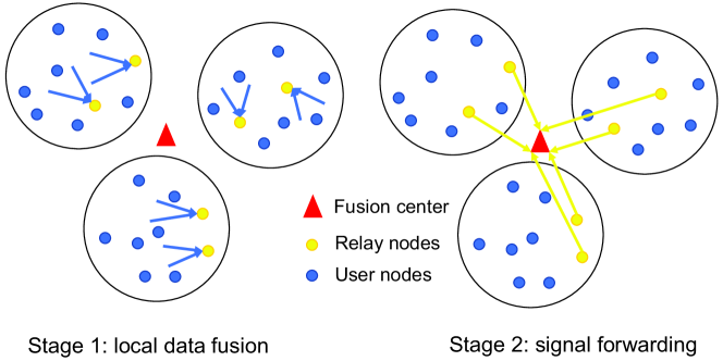
Figure 1: The illustration of cluster-based cooperation.

For simplicity of analysis, we make the following assumptions:

1. All the user clusters are of equal size $K_{C}$, i.e., $|{\mathbb{U}}^{(n)}_{1}|=|{\mathbb{U}}^{(n)}_{2}|\ldots=|{\mathbb{U}}^{(n)}_{C}|=K_{C}$.

2. The local decision fusion within each cluster is perfect.

3. The $L$ relays in any cluster are the same distance away from the FC, denoted by $r_{c}^{(n)}$. Moreover, $r_{c}^{(n)}$ are i.i.d. random variables with the pdf given in (2).

4. The FC has the instantaneous CSI of the channels between the relay nodes in each cluster and the FC, which is denoted by ${\mathbb{H}}^{(n)}_{c}:=\{{\bm{\rho}}^{(n)}_{c,1},{\bm{\rho}}^{(n)}_{c,2},\ldots,{\bm{\rho}}^{(n)}_{c,L}\}\,(c=1,2,\ldots,C)$. Here ${\bm{\rho}}^{(n)}_{c,l}:=\sqrt{P_{L}(r^{(n)}_{c})}|{\bm{h}}^{(n)}_{c,l}|\;(l=1,2,\ldots,L)$ are the channel gains and ${\bm{h}}^{(n)}_{c,l}\sim\mathcal{CN}(0,1)$ are the Rayleigh fading coefficients between relay $l$ and the FC. The FC makes the relay selection based on ${\mathbb{H}}^{(n)}_{c}$ and notifies the selected relay nodes.

Similar to (4), the received signal ${\bm{y}}$ can be written as

$${\bm{y}}[i]=\sum_{c=1}^{C}{\bm{\rho}}^{(n)}_{c}[i]\sqrt{P_{s}}\tilde{{\bm{s}}}^{(n)}_{c}[i]+{\bm{v}}^{(n)}[i],\;\;\;i=1,2,\ldots,d,$$

where ${\bm{\rho}}^{(n)}_{c}[i]\in{\mathbb{H}}^{(n)}_{c}\cup\{0\}$ depends on our relay selection scheme and ${\bm{v}}^{(n)}[i]\sim\mathcal{CN}(0,N_{0})$ is the i.i.d. additive white Gaussian noise.

It is worth noting that similar cluster-based methods have been applied to cooperative spectrum sensing to merge sensing observations from different users [8, 9]. However, their focuses are on the false alarm probability or energy efficiency while ours are on the failure probability that will be introduced in Section III.

III Failure Probability Analysis

Prior works have shown that the convergence speed of Algorithm 1 crucially depends on the decoding failure probability ${\bm{q}}^{(n)}[i]$ ($i=1,2,\ldots,d$) defined as

$${\bm{q}}^{(n)}[i]=\mathbf{Prob}\big{[}\tilde{{\bm{g}}}^{(n)}[i]\neq\operatorname{sign}\big{(}\nabla F({\bm{w}}^{(n)})[i]\big{)}\>|\>{\bm{w}}^{(n)}\big{]},$$ (8)

which is the probability that the result of majority vote mismatches the sign of the true gradient. In particular, smaller failure probability leads to a higher convergence speed, and increasing the number of participating users can attain similar speedup to distributed SGD [6]. In this section, we will discuss the failure probability of the digital AirComp-PC scheme proposed in Section II-B and show that wireless impairments effectively decrease the participating rate of voting users.

In our scheme, the failure probability depends on the following three factors:

1. The local success probability defined as

   $${\bm{p}}^{(n)}_{k}[i]:=\mathbf{Prob}\big{[}{\bm{s}}^{(n)}_{k}[i]=\operatorname{sign}\big{(}\nabla F({\bm{w}}^{(n)})[i]\big{)}\>|\>{\bm{w}}^{(n)}\big{]},$$

   which is the probability that the sign of the local stochastic gradient is the same as the sign of the true gradient;

2. The number of voting users $K$;

3. The wireless channel conditions between the FC and users.

We first discuss the local success probability. Intuitively, at the beginning stage of model training, the global loss function $F$ has a relatively large gradient at the point ${\bm{w}}^{(n)}$, and hence with high probability the sign of the local stochastic gradient is correct. As the model training proceeds, ${\bm{w}}^{(n)}$ will gradually approach the stationary point of $F$ and the true gradient will be close to zero. This means that the noise terms will dominate the local stochastic gradients resulting in almost random guess at each user. Therefore, we will set the local success probability to near 0.5 and focus on the other two factors in the following.

III-A Detection SNR

Because of symmetry, we only need to analyze the failure probability of a specific gradient component $\nabla F({\bm{w}}^{(n)})[i]$. Assume $\nabla F({\bm{w}}^{(n)})[i]>0$ without loss of generality. To simplify notation, we omit the superscript $(n)$ and the index $[i]$ in the following. The model can be now expressed as

$$y=\sum_{k=1}^{K}\rho_{k}s_{k}+v,$$ (9)

where $y$ is the received signal at the FC, $\rho_{k}$ is the channel coefficient between the FC and user $k$, $s_{k}\in\{+1,-1\}$ is the sign of the stochastic gradient at user $k$, and $v\sim\mathcal{N}(0,N_{0}/(2P_{s}))$ is the additive white Gaussian noise. By our assumptions, $\{s_{k}\}_{k=1}^{K}$ are independent from each other and $\mathbf{Prob}[s_{k}=1]=p_{k},\;\mathbf{Prob}[s_{k}=-1]=1-p_{k}$ where $p_{k}>1/2$. The failure probability is given by $q=\mathbf{Prob}{[y<0]}$.

We first assume the channel coefficients ${\bm{\rho}}$ are given parameters. In general, the closed form of $q$ is intractable. Hence, we provide an upper bound by using the properties of sub-Gaussian random variables [10].

Theorem 1.

Define

$$\tau^{2}:=\sum_{k=1}^{K}\rho_{k}^{2}+\frac{N_{0}}{2P_{s}}.$$ (10)

If $y$ is given by (9), then we have

$$q=\mathbf{Prob}({y<0})\leq\exp(-\frac{\mathbb{E}[y]^{2}}{2\tau^{2}}),$$ (11)

where

$$\mathbb{E}[y]=\sum_{k=1}^{K}\rho_{k}(2p_{k}-1).$$ (12)

Proof.

First recall the definition of sub-Gaussian random variables: a zero-mean random variable $X$ is sub-Gaussian with parameter $\theta$ if it satisfies $\mathbb{E}[\exp(tX)]\leq\exp(\frac{\theta^{2}t^{2}}{2})\;(\forall t\in\mathbb{R})$ and we write $X\in\mathrm{subG}(\theta^{2})$. We will use the following two key properties [10]:

1. If ${X}\in\mathrm{subG}(\theta^{2})$, then we have the tail bound $\mathbf{Prob}(X>x)\leq\exp(-\frac{x^{2}}{2\theta^{2}}),\;\forall x>0$.

2. Suppose $X_{1},X_{2},\ldots,X_{n}$ are $n$ independent random variables such that $X_{k}\in\mathrm{subG}(\theta_{k}^{2})$. Then the weighted sum satisfies $\sum_{k=1}^{n}a_{k}X_{k}\in\mathrm{subG}(\sum_{k=1}^{n}a_{k}^{2}\theta_{k}^{2})$.

We are now ready to prove (11). Since $v\sim\mathcal{N}(0,N_{0}/(2P_{s}))$, it is easy to verify $v\in\mathrm{subG}(N_{0}/(2P_{s}))$ by definition. Moreover, we can prove $s_{i}-\mathbb{E}[{s_{i}}]\in\mathrm{subG}(1)$ with Theorem 3.1 in [10]. Therefore, we can use property 2) to get $y-\mathbb{E}[y]\in\mathrm{subG}(\tau^{2})$, where $\tau^{2}$ is given in (10). Finally, property 1) leads to

$$q=\mathbf{Prob}(\mathbb{E}[y]-y>\mathbb{E}[y])\leq\mathrm{exp}(-\frac{\mathbb{E}[y]^{2}}{2\tau^{2}}).$$

∎

In BPSK detection, we may view $\mathbb{E}[y]^{2}$ and $\mathrm{Var}[y]$ as the signal and noise power respectively. Note that $\mathrm{Var}{[y]}=\sum_{k=1}^{K}4\rho_{k}^{2}p_{k}(1-p_{k})+N_{0}/(2P_{s})\leq\tau^{2}$ and the equality holds when $p_{1}=p_{2}=\ldots=p_{K}=1/2$. Hence, we refer to $\mathrm{SNR}_{\mathrm{d}}:=\mathbb{E}[y]^{2}/\tau^{2}$ as the detection SNR.

In the following, we assume that users have i.i.d. datasets and $p_{1}=p_{2}=\ldots=p_{K}=p_{\mathrm{loc}}$. The detection SNR becomes

$$\mathrm{SNR}_{\mathrm{d}}=(2p_{\mathrm{loc}}-1)^{2}\frac{\|{\bm{\rho}}\|_{1}^{2}}{\|{\bm{\rho}}\|_{2}^{2}+N_{0}/(2P_{s})}.$$ (13)

Note that for ideal noiseless channels where $N_{0}=0$ and $\rho_{1}=\rho_{2}=\ldots=\rho_{K}=1$, we have $\mathrm{SNR}_{\mathrm{d}}=(2p_{\mathrm{loc}}-1)^{2}K$. This motivates us to define the normalized detection SNR as

$$\overline{\mathrm{SNR}}_{\mathrm{d}}=\frac{1}{K}\frac{\|{\bm{\rho}}\|_{1}^{2}}{\|{\bm{\rho}}\|_{2}^{2}+N_{0}/(2P_{s})}.$$ (14)

The advantage of dealing with $\overline{\mathrm{SNR}}_{\mathrm{d}}$ is that it depends only on the channels between the FC and users but not on $p_{\mathrm{loc}}$. Furthermore, we have the following result:

Proposition 1.1.

If $\overline{\mathrm{SNR}}_{\mathrm{d}}$ is given by (14), then

$$0\leq\overline{\mathrm{SNR}}_{\mathrm{d}}\leq 1,$$

where the second equality holds if and only if $N_{0}=0$ and $\rho_{1}=\rho_{2}=\ldots=\rho_{K}$.

Proof.

We omit the proof due to space limitations. ∎

Since $\mathrm{SNR}_{\mathrm{d}}$ is proportional to the number of users $K$ for ideal noiseless channels, we can interpret $\overline{\mathrm{SNR}}_{\mathrm{d}}$ as the effective participation rate of users.

III-B Simulation Validations

In our model, we have $\rho_{k}=\sqrt{P_{L}(r_{k})}|h_{k}|$ where $h_{k}\sim\mathcal{CN}(0,1)$ i.i.d., the pdf of $r_{k}$ is given by (2), and $P_{L}(\cdot)$ is given by (3). When $K$ is sufficiently large, we can approximate $\overline{\mathrm{SNR}}_{\mathrm{d}}$ by the law of large numbers:

$$\overline{\mathrm{SNR}}_{\mathrm{d}} \approx\frac{(\mathbb{E}[|h_{k}|]\mathbb{E}[\sqrt{P_{L}(r_{k})}])^{2}}{\mathbb{E}[|h_{k}|^{2}]\mathbb{E}[P_{L}(r_{k})]+N_{0}/(2KP_{s})}$$

$$=\frac{\pi/4\;\mathbb{E}[\sqrt{P_{L}(r_{k})}]^{2}}{\mathbb{E}[P_{L}(r_{k})]+N_{0}/(2KP_{s})},$$ (15)

where

$$\mathbb{E}[\sqrt{P_{L}(r_{k})}] =-\frac{\alpha}{4-\alpha}\left(\frac{r_{0}}{R}\right)^{2}+\frac{4}{4-\alpha}\left(\frac{r_{0}}{R}\right)^{\frac{\alpha}{2}},$$

$$\mathbb{E}[{P_{L}(r_{k})}] =-\frac{\alpha}{2-\alpha}\left(\frac{r_{0}}{R}\right)^{2}+\frac{2}{2-\alpha}\left(\frac{r_{0}}{R}\right)^{{\alpha}}.$$

From (15) we can see that when $2KP_{s}\mathbb{E}[{P_{L}(r_{k})}]/N_{0}\gg 1$ the channel noise is negligible. Therefore, when the symbol power $P_{s}$ exceeds a certain threshold, $\overline{\mathrm{SNR}}_{\mathrm{d}}$ will reach the maximum and remain unchanged. We can observe such phenomenon from the left figure in Fig. 2: with increasing $P_{s}$, the failure probability will decrease until reaching the error floor. This may be explained by the fact that the users’ signals are coherently combined at the FC, resulting in a power gain similar to transmit beamforming. From the above, we conclude that channel noise is not the bottleneck for digital AirComp-PC at a reasonably large SNR.

Moreover, by Theorem 1 we have $q\leq\exp(-K\overline{\mathrm{SNR}}_{\mathrm{d}})$, meaning that the failure probability decays at an exponential rate. However, there exists a huge gap between the digital AirComp-PC and the ideal majority vote, which is more evident when $K$ increases. For instance, when $\alpha=3$ and $R/r_{0}=30$, from (15) we get ${\overline{\mathrm{SNR}}{}}_{\mathrm{d}}\approx 10.6\%$. This shows that equivalently about only 10.6% of users participate. In the right figure in Fig. 2, We also plot the failure probability of the equivalent ideal majority vote (the dash line), which is indeed close to the actual performance of the digital AirComp-PC.

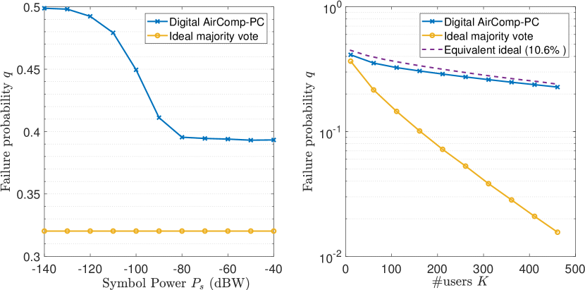
Figure 2: The left figure shows the failure probability $q$ versus symbol power $P_{s}$ where $K=21,\,p_{\mathrm{loc}}=0.55$, $\alpha=3$ and $R/r_{0}=30$ in (3). The right figure shows $q$ versus the number of users $K$ where $P_{s}=-50$dBW and other parameters are the same as the left.

IV Relay Selection Scheme

To design the relay selection scheme in Section II-C, we use the normalized detection SNR as the optimization objective to minimize the failure probability. As in Section III, we omit the superscript and the index. The channel model becomes

$$y=\sum_{c=1}^{C}\rho_{c}\tilde{s}_{c}+v,$$

where $\rho_{c}\in{\mathbb{H}}_{c}\cup\{0\}$ depends on our relay selection scheme; $\tilde{s}_{c}=\operatorname{sign}(\sum_{k\in{\mathbb{U}}_{c}}s_{k})$ is the majority vote result within cluster ${\mathbb{U}}_{c}$ and $\mathbf{Prob}[s_{k}=1]=p_{\mathrm{loc}},\,\mathbf{Prob}[s_{k}=-1]=1-p_{\mathrm{loc}},\,p_{\mathrm{loc}}>1/2$; and $v\sim\mathcal{N}(0,N_{0}/(2P_{s}))$ is the additive white Gaussian noise.

When the number of users $K_{c}$ within each cluster is sufficiently large, by law of large numbers we have

$$\tilde{s}_{c}=\frac{\sum_{k\in{\mathbb{U}}_{c}}s_{k}}{|\sum_{k\in{\mathbb{U}}_{c}}s_{k}|}\approx\frac{\sum_{k\in{\mathbb{U}}_{c}}s_{k}}{K_{C}(2p_{\mathrm{loc}}-1)}.$$

Hence, the normalized detection SNR can be approximated by

$${\overline{\mathrm{SNR}}}_{\mathrm{d}} =\frac{1}{C}\frac{\left(\sum_{c=1}^{C}\rho_{c}\right)^{2}}{\sum_{c=1}^{C}\rho_{c}^{2}+K_{C}(2p_{\mathrm{loc}}-1)^{2}N_{0}/(2P_{s})}$$

$$\approx\frac{1}{C}\frac{\left(\sum_{c=1}^{C}{\rho_{c}}\right)^{2}}{\sum_{c=1}^{C}\rho_{c}^{2}},$$ (16)

where we discard the noise term in (16). From the discussion in Section III-B, we know that the channel noise is negligible for SNR at a reasonable level. The relay selection can be formulated as the following optimization problem:

$$\max_{\rho_{1},\rho_{2},\ldots,\rho_{C}} \frac{1}{C}\frac{\left(\sum_{c=1}^{C}{\rho_{c}}\right)^{2}}{\sum_{c=1}^{C}\rho_{c}^{2}}$$ (17)

$$\mathrm{s.t.} \rho_{c}\in\{\rho_{c,1},\ldots,\rho_{c,L}\}\cup\{0\},$$

where $\rho_{c}=0$ corresponds to the case when no relay in cluster ${\mathbb{U}}_{c}$ participates. This is a typical discrete optimization problem with $(L+1)^{C}$ feasible solutions in total. Therefore, we consider two low-complexity relay selection schemes.

One approach is to select the relay with the strongest gain:

$$\rho_{c}=\max\{\rho_{c,1},\ldots,\rho_{c,L}\},\;c=1,2,\ldots,C.$$

We refer to it as the strongest gain scheme. However, in the context of digital AirComp-PC, this is far from optimal. Intuitively, because of the randomness of users’ locations, the large-scale fading effects vary greatly among the clusters. Hence, the signal sent by the relay close to the FC will drown out the signals from other relays, resulting in the loss of effective voting users.

Algorithm 2 Iterative greedy algorithm for  (17)

1:Input: ${\mathbb{H}}_{c}=\{\rho_{c,1},\ldots,\rho_{c,L}\},\;c=1,2,\ldots,C$

2:Initialize $\rho_{c}\leftarrow\max\{\rho_{c,1},\ldots,\rho_{c,L}\},\;c=1,2,\ldots,C$

3:repeat

4:     for $c=1,2,\ldots,C$ do

5:         $a\leftarrow\sum_{k\neq c}\rho_{k},\;b\leftarrow\sum_{k\neq c}\rho_{k}^{2}$

6:         $\rho_{c}\leftarrow\operatorname*{arg\,min}_{\rho\in{\mathbb{H}}_{c}\cup\{0\}}|\frac{1}{\rho+a}-\frac{a}{a^{2}+b}|$

7:     end for

8:until $\{\rho_{1},\rho_{2},\ldots,\rho_{C}\}$ are unchanged

To mitigate such drawback, we propose an iterative greedy algorithm as shown in Algorithm 2. We first use the strongest gain scheme to initialize $\rho_{1},\rho_{2},\ldots,\rho_{C}$. Then we successively optimize one variable at a time while keeping the others fixed and repeat the process until all the variables no longer change. We can see that the objective value is non-decreasing after every iteration. Since there are only finite feasible solutions, Algorithm 2 is guaranteed to terminate in finite steps.

We run numerical experiments to compare the strongest gain scheme with the iterative greedy algorithm and plot the results in Fig. 3. When user clustering and relay selection are adopted, we can see a substantial improvement upon the digital AirComp-PC without cooperation. Moreover, the iterative greedy algorithm attains a much lower failure probability than the strongest gain scheme, and is close to the ideal case when $L=5$. Together with the discussion in Section III-B, this shows that our cluster-based cooperation scheme can effectively increase the participation rate of voting users.

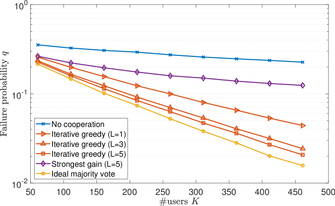
Figure 3: The failure probability versus number of users with a fixed size of cluster $K_{C}=9$. The other parameters are the same as in Fig. 2.

V Simulation Results

We evaluate our relay selection schemes in an edge learning system with $K=54$ users. The cell radius is $R=1000$ m, path loss exponent $\alpha=3$, and $r_{0}=10$ m in (3). The number of subchannels is $M=1000$ and 4-QAM is adopted. The symbol power budget is $P_{s}=-50$ dBW and the noise variance $N_{0}=80$ dBm. We consider the MNIST digit recognition problem and use Algorithm 1 to train a multilayer perceptron (MLP) with one hidden layer of 64 units using ReLu activations. The training samples are distributed uniformly at random. In our cooperative scheme, we assume there are $C=6$ clusters each containing $K_{C}=9$ users.

As shown in Fig. 4, the relay selection scheme with the iterative greedy algorithm achieves a very similar performance as the ideal majority vote. The difference of their final test accuracies is smaller than 0.5%. In contrast, the system without cooperation converges more slowly and its final test accuracy is near $1.2$% less than the ideal case. This shows that user clustering and relay selection can effectively combat the channel fading impairments.

We also test the idea that the normalized SNR in (14) can be regarded as the participation rate of voting users. By Monte Carlo simulations, we obtain that the normalized SNR is around 0.32 in the system without cooperation. From our discussion in Section III-A, the number of effective users is $54\times 0.32\approx 17$. Therefore, we also plot the test accuracy for ideal majority vote when $K=17$ (the dash line). We can see that the performance is indeed close to that of the system without cooperation, which is consistent with our analysis.

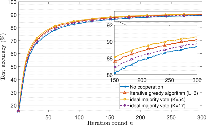
Figure 4: Test accuracy while training a MLP on MNIST dataset. The curves are the average results of 5 repeats.

VI Conclusions

We proposed a new digital AirComp scheme for federated edge learning systems that has less stringent requirements on the transmitters. To characterize the failure probability of majority vote in our scheme, we derived an upper bound and defined the normalized detection SNR. We found that the impact of wireless fading is equivalent to decreasing the number of voting users. Furthermore, we designed a cluster-based cooperation scheme to combat wireless impairments and proposed relay selection schemes based on the normalized detection SNR. Simulations show that the relay selection scheme with the iterative greedy algorithm can well exploit spatial diversity and achieve a comparable convergence speed to the system with ideal channels.

References

- [1] G. Zhu, D. Liu, Y. Du, C. You, J. Zhang, and K. Huang, “Toward an intelligent edge: Wireless communication meets machine learning,” IEEE Communications Magazine, vol. 58, no. 1, pp. 19–25, 2020.
- [2] H. B. McMahan, E. Moore, D. Ramage, S. Hampson, and B. A. y Arcas, “Communication-efficient learning of deep networks from decentralized data,” in Artificial Intelligence and Statistics, 2017, pp. 1273–1282.
- [3] G. Zhu, Y. Wang, and K. Huang, “Broadband analog aggregation for low-latency federated edge learning,” IEEE Transactions on Wireless Communications, vol. 19, no. 1, pp. 491–506, 2020.
- [4] M. M. Amiri and D. Gündüz, “Federated learning over wireless fading channels,” IEEE Transactions on Wireless Communications, vol. 19, no. 5, pp. 3546–3557, 2020.
- [5] G. Zhu, Y. Du, D. Gunduz, and K. Huang, “One-bit over-the-air aggregation for communication-efficient federated edge learning: Design and convergence analysis,” arXiv preprint arXiv:2001.05713, 2020.
- [6] J. Bernstein, Y.-X. Wang, K. Azizzadenesheli, and A. Anandkumar, “signsgd: compressed optimisation for non-convex problems,” in ICML 2018: Thirty-fifth International Conference on Machine Learning, 2018, pp. 559–568.
- [7] B. Chen, R. Jiang, T. Kasetkasem, and P. Varshney, “Channel aware decision fusion in wireless sensor networks,” IEEE Transactions on Signal Processing, vol. 52, no. 12, pp. 3454–3458, 2004.
- [8] C. Sun, W. Zhang, and K. B. Letaief, “Cluster-based cooperative spectrum sensing in cognitive radio systems,” in 2007 IEEE International Conference on Communications, 2007, pp. 2511–2515.
- [9] C. Lee and W. Wolf, “Energy efficient techniques for cooperative spectrum sensing in cognitive radios,” in 2008 5th IEEE Consumer Communications and Networking Conference, 2008, pp. 968–972.
- [10] V. V. Buldygin and K. K. Moskvichova, “The sub-gaussian norm of a binary random variable,” Theory of Probability and Mathematical Statistics, vol. 86, pp. 33–49, 2013.