Thermoelectric detection of Andreev states in unconventional superconductors

Abstract

We theoretically describe a thermoelectric effect that is entirely due to Andreev processes involving the formation of Cooper pairs through the coupling of electrons and holes. The Andreev thermoelectric effect can occur in ballistic ferromagnet-superconductor junctions with a dominant superconducting proximity effect on the ferromagnet, and it is very sensitive to surface states emerging in unconventional superconductors. We consider hybrid junctions in two and three dimensions to demonstrate that the thermoelectric current is always reversed in the presence of low-energy Andreev bound states at the superconductor surface. A microscopic analysis of the proximity-induced pairing reveals that the thermoelectric effect only arises if even and odd-frequency Cooper pairs coexist in mixed singlet and triplet states. Our results are an example of the richness of emergent phenomena in systems that combine magnetism and superconductivity, and they open a pathway for exploring exotic surface states in unconventional superconductors.

I Introduction

Thermoelectric effects, where temperature gradients and electric voltages are converted into each other, open a promising way to reuse waste heat in electronic devices Bauer et al. (2012). In mesoscopic conductors, a thermoelectric current can be generated by breaking the electron-hole symmetry around the chemical potential. However, the current is usually small at low temperatures. By contrast, large thermoelectric effects have recently been predicted Kalenkov et al. (2012); Ozaeta et al. (2014); Machon et al. (2014) and measured Kolenda et al. (2016, 2017) in hybrid junctions between superconductors and magnetic materials. The novel field of superconducting spintronics Eschrig (2011); Linder and Robinson (2015); Eschrig (2015) explores such phenomena that arise due to the interplay between superconductivity and magnetism Keizer et al. (2006); Khaire et al. (2010); Robinson et al. (2010a, b); Yang et al. (2010); Hübler et al. (2012). Interestingly, by coupling the spin degree of freedom to the heat (or charge) transport in ferromagnet-superconductor hybrid junctions, it may be possible to develop more efficient thermoelectric devices Giazotto et al. (2014, 2015a); Paolucci et al. (2018), such as coolers Machon et al. (2014); Ozaeta et al. (2014); Sánchez et al. (2018) and thermometers Giazotto et al. (2015b).

Many of these applications are based on conventional superconductors with $s$-wave, spin-singlet pair potentials Bergeret et al. (2018). By contrast, in unconventional superconductors Kashiwaya and Tanaka (2000); Löfwander et al. (2001), Cooper pairs couple via anisotropic channels, like $d$-wave Hu (1994); Tanaka and Kashiwaya (1995); Kashiwaya et al. (1996); Tanaka and Kashiwaya (1996a), or form spin-triplet states Buchholtz and Zwicknagl (1981); Yamashiro et al. (1997); Mackenzie and Maeno (2003); Maeno et al. (2012); Kallin (2012). One intriguing aspect of unconventional superconductors is the possibility to develop surface Andreev bound states (SABS), which occur due to the anisotropy of the pair potentials. These edge states can be topologically protected Read and Green (2000); Ryu and Hatsugai (2002); Sato et al. (2011) and may play the role of Majorana states in condensed matter Kallin and Berlinsky (2016); Sato and Ando (2017); Sato and Fujimoto (2016); Aguado (2017). SABS are also related to point or line nodes where the pairing potential vanishes Kobayashi et al. (2015); Tamura et al. (2017), often leading to a pronounced zero-bias peak in the tunneling conductance Hu (1994); Matsumoto and Shiba (1995); Tanaka and Kashiwaya (1995); Löfwander et al. (2001), like the ones observed in, e.g., high-$T_{c}$ cuprates Covington et al. (1997a); *Greene_1997err; Alff et al. (1997); Wei et al. (1998); Kashiwaya et al. (1998); Iguchi et al. (2000); Biswas et al. (2002); Chesca et al. (2008).

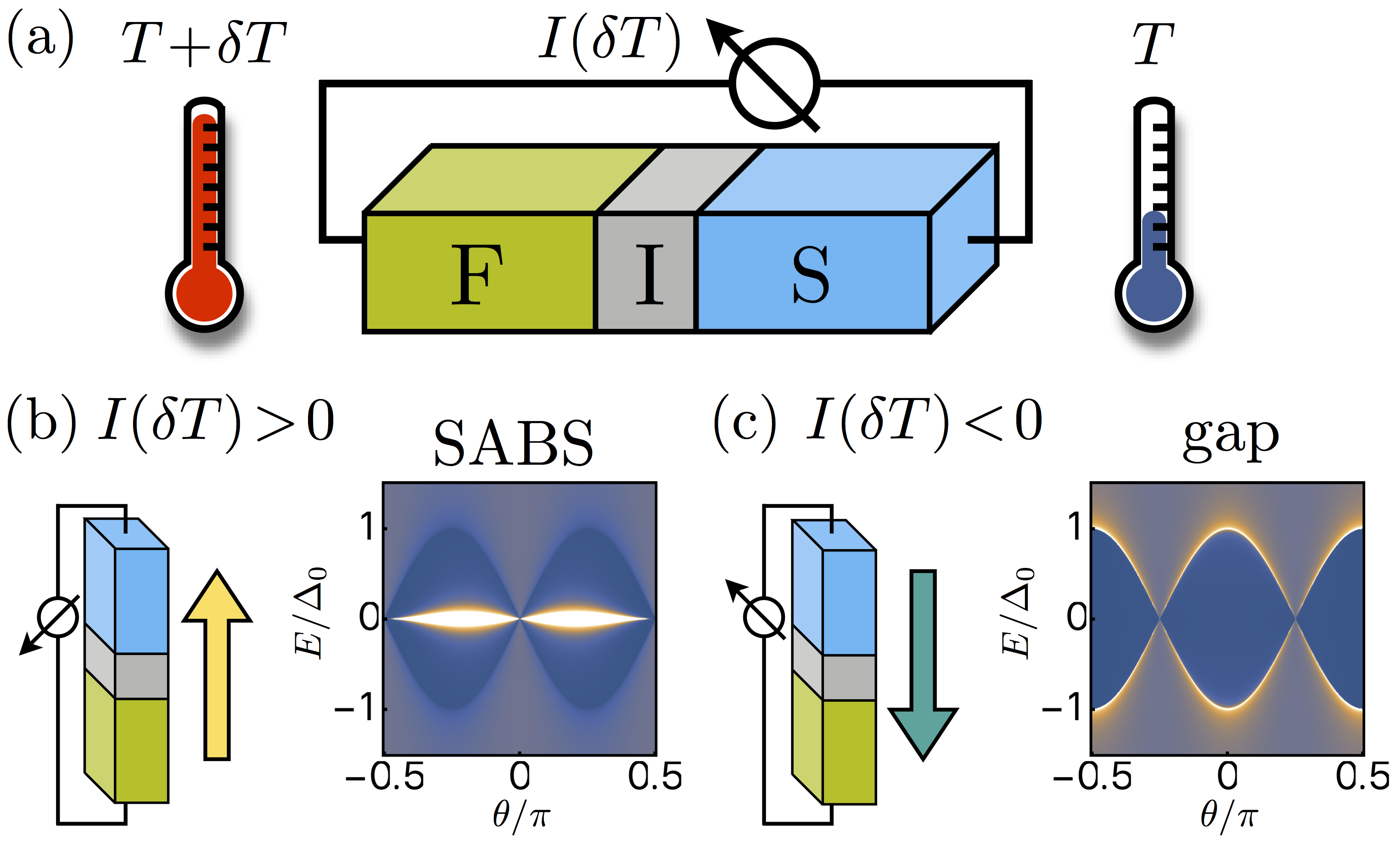
Figure 1: Thermoelectric effect and direction of the current in a ferromagnet-superconductor hybrid junction. (a) Setup indicating the hot and cold reservoirs. (b,c) Assuming a majority of spin-up particles, a positive thermoelectric current flows into the superconductor (b) in the presence of SABS, while a negative one runs out of it in their absence (c).

Here, we analyze the electrical current induced by a temperature gradient across hybrid junctions involving unconventional superconductors in two and three dimensions, see Fig. 1. The thermoelectric effect has been measured in ferromagnet-superconductor tunnel junctions under an external magnetic field Kolenda et al. (2016) or in proximity to a ferromagnetic insulator Kolenda et al. (2017). For this reason, we concentrate here on the transport properties of ballistic ferromagnet–insulator–superconductor (F-I-S) and ferromagnet–ferromagnetic-insulator–superconductor (F-Fi-S) junctions described by scattering theory Blonder et al. (1982); Tanaka and Kashiwaya (1995); Kashiwaya and Tanaka (2000). Building on earlier work on the spin and charge transport of F-I-S junctions with unconventional pairings Fogelström et al. (1997); Kashiwaya et al. (1999); Žutić and Valls (1999, 2000); Yoshida et al. (2000); Tanuma et al. (2002a, b); Tanaka et al. (2002); Hirai et al. (2003); Tanaka et al. (2009), we show that the thermoelectric current is dominated by Andreev processes, where electrons and holes are converted into each other at the surface of the superconductor. Interestingly, the thermoelectric current changes sign in the presence of SABS: it is positive (it runs into the superconductor) when the conductance features a zero-bias peak and it is negative otherwise, as illustrated in Fig. 1(b,c).

Earlier predictions of the thermoelectric effect in ferromagnet-superconductor junctions require that the exchange field from the magnet penetrates the superconductor, and thereby spin-splits its density of states Bergeret et al. (2018). Such a magnetic (or inverse) proximity effect can be achieved in thin films of conventional superconductors Hübler et al. (2012); Quay et al. (2013), which could be challenging to implement with unconventional ones. Our results, by contrast, rely on the coupling between the ferromagnet’s exchange field and the Cooper pairs leaking out of the superconductor. When the superconducting proximity effect takes place Lu et al. (2016); *Lu_2017, quasiparticles can tunnel into the superconductor only when the pairing rotational symmetry is broken at the interface. However, this additional contribution to the thermoelectric current is always smaller than the Andreev one for pairings featuring zero-bias peaks, and hence it does not affect the direction of the current flow. An analysis of the proximity-induced pair amplitude at the junction interface, based on Green’s function techniques, allows us to show that the Andreev thermoelectric current is only possible when even- and odd-frequency Cooper pairs coexist Tanaka and Golubov (2007); Eschrig et al. (2007); Tanaka et al. (2007a, b, 2012). The thermoelectric effect is thus a signature of proximity-induced odd-frequency pairing, and it thereby becomes a sensitive tool to explore unconventional superconductivity.

The rest of the paper is organized as follows. We introduce the theoretical methods in Section II and explain the Andreev thermoelectric effect and the current sign change in Section III. In Section IV, we use Green’s function techniques to analyze the proximity-induced pairing on the ferromagnetic region. Section V discusses the quasiparticle contribution to the thermoelectric current. Finally, we present our conclusions in Section VI.

II Theoretical formulation

We consider ballistic junctions between a superconductor and a magnetic normal-state metal separated by an insulating barrier. Transport takes place in the $x$-direction, with the superconductor extending over the region $x\geq 0$. In all cases below, we assume perfectly flat and clean interfaces. Transport in such junctions is described by the Bogoliubov-de Gennes (BdG) equations

$$\check{H}\Psi=E\Psi,$$ (1)

with $E$ being the excitation energy. Particle-hole symmetry imposes that every solution $\Psi_{E}$ of the BdG equations with excitation energy $E$ is accompanied by another solution, $\Psi_{-E}$, at energy $-E$. We then choose the basis

$$\Psi\!=\![\hat{c}_{\uparrow}(\mathbf{k}),\hat{c}_{\downarrow}(\mathbf{k}),\hat{c}^{\dagger}_{\uparrow}(-\mathbf{k}),\hat{c}^{\dagger}_{\downarrow}(-\mathbf{k})]^{T}$$ (2)

in Nambu (particle-hole) and spin space, with $\hat{c}_{\sigma}(\mathbf{k})$ being the annihilation operator for an electron with spin $\sigma\!=\uparrow,\downarrow$ and momentum $\mathbf{k}$. The general form of the BdG Hamiltonian in any region is

$$\check{H}(\mathbf{k})=\left(\!\begin{array}[]{cc}\hat{h}(\mathbf{k})\!-\!\mu\hat{\sigma}_{0}&\hat{\Delta}(\mathbf{k})\mathrm{e}^{i\phi}\\ \hat{\Delta}^{\dagger}(\mathbf{k})\mathrm{e}^{-i\phi}&\mu\hat{\sigma}_{0}\!-\!\hat{h}^{*}(-\mathbf{k})\end{array}\!\right),$$ (3)

where $\hat{\sigma}_{0,1,2,3}$ are the usual Pauli matrices in spin space and $\mu$ and $\hat{\Delta}$ the chemical and pair potentials, respectively. It is reasonable to assume that these quantities are constant in each region. For the sake of simplicity, we take the same value of the chemical potential on both sides of the junction. The pair potential is zero in the normal region, which is a good approximation if the superconducting coherence length is much larger than the Fermi wavelength. The superconducting phase $\phi$ only plays a role in junctions with several superconductors, hence, we omit it here.

In the following we consider systems in either two or three dimensions with the single-particle Hamiltonian

$$\hat{h}(\mathbf{r})=-\frac{\hbar^{2}\mathbf{\nabla}^{2}}{2m}\hat{\sigma}_{0}-U(x)\hat{\sigma}_{3}+\left(V_{0}\hat{\sigma}_{0}+U_{\text{B}}\hat{\sigma}_{3}\right)\delta(x),$$ (4)

where $m$ is the electron mass and $U(x)=U_{0}\Theta(-x)$ is the exchange potential in the normal-state region with $U_{0}\geq 0$ and $\Theta(x)$ being the Heaviside step function. The potential $V_{0}$ describes the insulating barrier at the interface with $U_{\text{B}}$ accounting for the exchange potential of ferromagnetic insulators. Assuming translational invariance in the plane perpendicular to the direction of transport, $\mathbf{r}_{\parallel}=(y,z)$, the momentum parallel to it, $\mathbf{k}_{\parallel}=(k_{y},k_{z})$, becomes a good quantum number. For a given incident wave, all related wave vectors lie in the same plane, see Fig. 2(a). We can then choose the coordinate system so that transport depends only on the azimuthal angle $\theta\!=\!\sin^{-1}(|\mathbf{k}_{\parallel}|/k_{\text{F}})$, where $k_{\text{F}}=\sqrt{2m\mu}/\hbar$ is the Fermi wave vector.

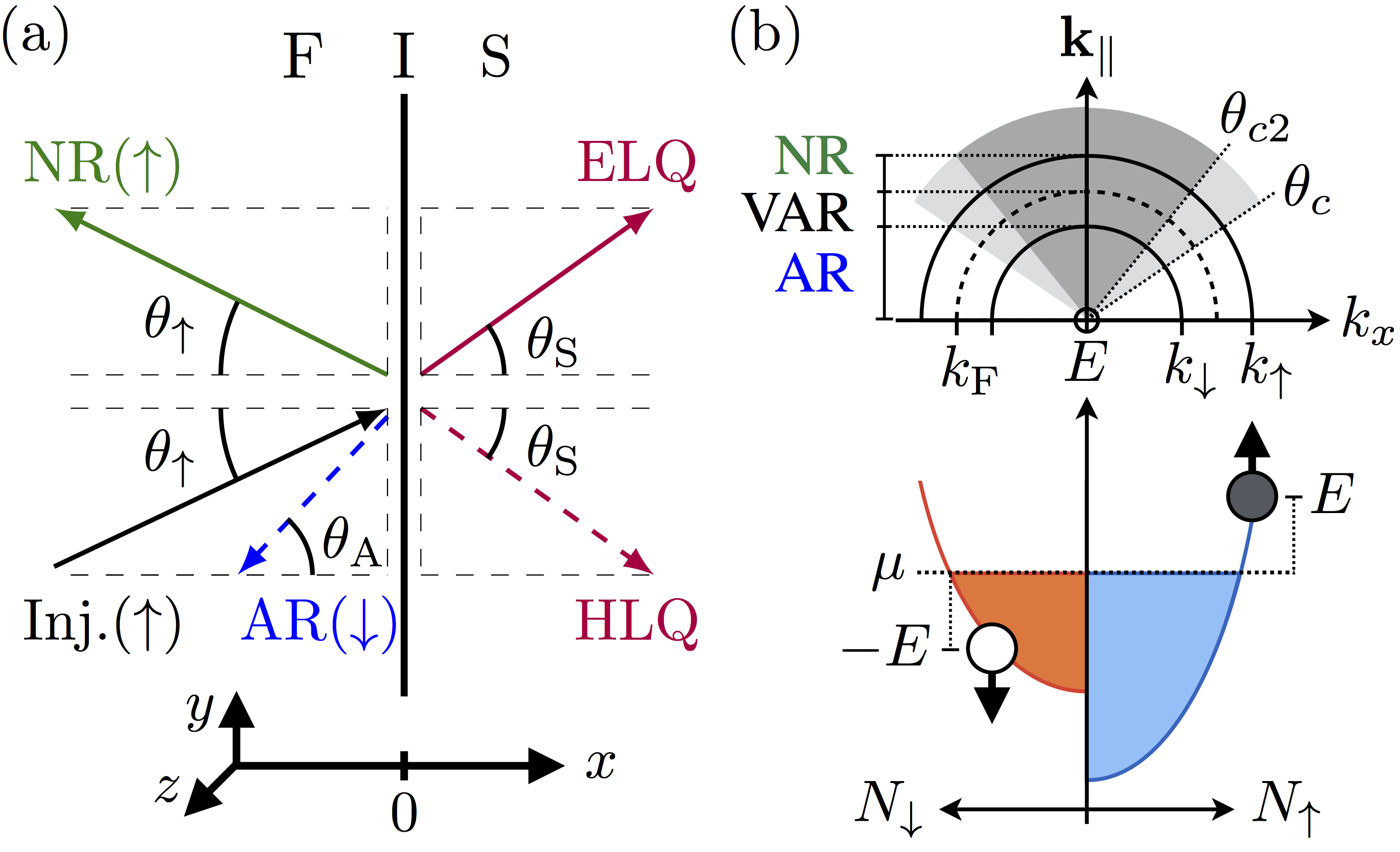
Figure 2: Andreev reflection in F-I-S junctions. (a) An electron incident from the ferromagnet can be normal-reflected (NR), Andreev reflected (AR), or transmitted as an electron- (ELQ) or hole-like (HLQ) quasiparticle. (b) Momentum (top) and energy (bottom) schematics of an Andreev reflection process. Assuming $k_{\uparrow}>k_{\text{F}}>k_{\downarrow}$, Andreev reflection is only possible for angles of incidence below a critical value $|\theta|<\theta_{c}$, virtual Andreev reflections (VAR) take place for $\theta_{c}<|\theta|<\theta_{c2}$, and all incident particles are backscattered for $|\theta|>\theta_{c2}$.

Inserting Eq. 4 into Eq. 3, the BdG equations can be decoupled into two spin channels if the pair potential $\hat{\Delta}$ is either a diagonal or an off-diagonal matrix, i.e., proportional to $\hat{\sigma}_{0,3}$ or $\hat{\sigma}_{1,2}$, respectively. The spin-singlet state, $\hat{\Delta}(\mathbf{k})\!=\!\Delta_{0}(\mathbf{k})(i\hat{\sigma}_{2})$ always fulfills this condition. The triplet state, which we parametrize as $\hat{\Delta}(\mathbf{k})\!=\!\mathbf{d}(\mathbf{k})\cdot\mathbf{\hat{\sigma}}(i\hat{\sigma}_{2})$, with $\mathbf{\hat{\sigma}}$ being a vector of Pauli matrices, fulfills the condition if $\mathbf{d}$ lies either along the $z$-axis or in the $x$-$y$ plane. In the following, we only consider pair potentials that fulfill these conditions and that couple electrons with opposite spins. Therefore, the injected and Andreev reflected particles have opposite spins and, if $U_{0}\neq 0$, Andreev retro-reflection does not take place Kashiwaya et al. (1999). Following a quasiclassical approximation, where the magnitude of the wave vectors is evaluated at the Fermi surface, translational symmetry at the interface entails that

$$k_{\sigma}\sin\theta=k_{\text{F}}\sin\theta_{\text{S}}=k_{\bar{\sigma}}\sin\theta_{\text{A}}^{\sigma},$$ (5)

where $k_{\sigma}=k_{\text{F}}\sqrt{1+\rho X}$, with $X=U_{0}/\mu$ being the polarization from the exchange field and $\rho=1\,(-1)$ and $\bar{\sigma}=\downarrow(\uparrow)$, when $\sigma=\uparrow(\downarrow)$. Consequently, assuming up-spin injection and $X>0$, total (normal) reflection takes place for $\theta>\sin^{-1}(k_{\text{F}}/k_{\uparrow})\equiv\theta_{\text{c}2}$, when $k_{\text{F}}\!<\!k_{\uparrow}$, and the Andreev-reflected wave becomes evanescent for the angles $\theta_{\text{c}2}>\theta>\sin^{-1}(k_{\downarrow}/k_{\uparrow})\equiv\theta_{\text{c}}$, if $k_{\downarrow}<k_{\text{F}}<k_{\uparrow}$. The latter case corresponds to virtual Andreev reflections Kashiwaya et al. (1999), which do not contribute to the current, see Fig. 2.

For a given spin channel $\sigma$, the general solution for the decoupled BdG equations is given by

$$\Psi_{\sigma}(x,\mathbf{r}_{\parallel})=\psi_{\sigma}(x)\mathrm{e}^{i\mathbf{k}_{\parallel}\cdot\mathbf{r}_{\parallel}},$$ (6)

where we have defined

$$\begin{split}\psi_{\sigma}(x)=\sum\limits_{\alpha=\pm}&\left[m^{\alpha}_{\sigma}\begin{pmatrix}1\\ (\eta^{\alpha}_{\sigma})^{*}\Gamma_{\sigma}^{\alpha}\end{pmatrix}\mathrm{e}^{ik_{e,\sigma}^{\alpha}\cos\theta_{\alpha}x}\right.\\ &\left.+\tilde{m}^{\alpha}_{\sigma}\begin{pmatrix}\eta^{\alpha}_{\sigma}\Gamma_{\sigma}^{\alpha}\\ 1\end{pmatrix}\mathrm{e}^{ik_{h,\sigma}^{\alpha}\cos\theta^{\prime}_{\alpha}x}\right],\end{split}$$ (7)

with $m^{\alpha}_{\sigma}$ ($\tilde{m}^{\alpha}_{\sigma}$) being the amplitude for an electron-like (hole-like) quasiparticle with direction of propagation $\alpha=\pm$. Here, $\theta_{+}\!=\!\theta$ and $\theta_{-}=\pi-\theta$ label right and left movers, respectively, and we have defined $\eta_{\sigma}^{\alpha}\!=\!\Delta^{\alpha}_{\sigma}/|\Delta^{\alpha}_{\sigma}|$, $\Gamma_{\sigma}^{\alpha}\!=\!|\Delta^{\alpha}_{\sigma}|/(E+\Omega_{\sigma}^{\alpha})$, and

$$\Omega_{\sigma}^{\alpha}=\left\{\begin{array}[]{cr}\operatorname{sgn}(E)\sqrt{E^{2}-|\Delta^{\alpha}_{\sigma}|^{2}}&,|E|>|\Delta^{\alpha}_{\sigma}|\\ i\sqrt{|\Delta^{\alpha}_{\sigma}|^{2}-E^{2}}&,|E|\leq|\Delta^{\alpha}_{\sigma}|\end{array}\right.,$$ (8)

where $k_{\text{e(h)},\sigma}^{\alpha}=k_{\text{F}}\sqrt{1+(-)\Omega_{\sigma}^{\alpha}/\mu+(-)\rho X}$ and $\Delta^{\alpha}_{\sigma}=\Delta_{\sigma}(\theta_{\alpha})$ is the pair potential felt by an $\alpha$-moving particle in spin channel $\sigma$.

Figure 2(a) shows the scattering of an electron incident from the normal-state region into an Andreev reflected hole (AR), a normal reflected electron (NR), an electron-like quasiparticle transmitted to the superconductor (ELQ), or a hole-like transmitted quasiparticle (HLQ). The reflection amplitudes are obtained evaluating the wave function in Eq. 7 for this scattering process and imposing the boundary conditions

$$\psi_{\sigma}(0^{-})={} \psi_{\sigma}(0^{+}),$$ (9a)

$$k_{\text{F}}\hat{Z}\psi_{\sigma}(0^{-})={} \left.\partial_{x}\psi_{\sigma}\right|_{x=0^{+}}-\left.\partial_{x}\psi_{\sigma}\right|_{x=0^{-}},$$ (9b)

with

$$\hat{Z}=Z_{0}\hat{\sigma}_{0}+Z_{m}\hat{\sigma}_{3}=2m(V_{0}\hat{\sigma}_{0}+U_{\text{B}}\hat{\sigma}_{3})/(\hbar^{2}k_{\text{F}}).$$ (10)

When solving Eq. 9, we follow the Andreev approximation, discarding terms of order $E/\mu$ and $\Delta_{0}/\mu$, resulting in $k_{\text{e(h)},\sigma}^{\alpha}\approx k_{\text{F}}$ in the superconducting region ($x>0$) and $k_{\text{e(h)},\sigma}^{\alpha}\approx k_{\sigma(\bar{\sigma})}$ for $x<0$. Accordingly, for the scattering of an incident electron with spin $\sigma$ the angles in Eq. 7 become $\theta=\theta^{\prime}=\theta_{\text{S}}$, for $x>0$, and $\theta$ and $\theta^{\prime}=\theta^{\sigma}_{\text{A}}$ for $x<0$.

The angle-resolved conductance per spin reads Blonder et al. (1982); Kashiwaya et al. (1999)

$$\sigma_{\sigma}(E,\mathbf{k}_{\parallel})=1-|b_{\sigma}|^{2}+\lambda_{\sigma}|a_{\sigma}|^{2}\equiv 1-B_{\sigma}+A_{\sigma},$$ (11)

where $a_{\sigma}(E,\mathbf{k}_{\parallel})$ and $b_{\sigma}(E,\mathbf{k}_{\parallel})$ are the Andreev and normal reflection amplitudes, respectively, and we have defined $\lambda_{\sigma}\!=\!\mathrm{Re}\{k_{\bar{\sigma}}\cos\theta_{\text{A}}^{\sigma}/(k_{\sigma}\cos\theta)\}$ and $\theta_{\text{A}}^{\sigma}\!=\!\sin^{-1}(k_{\sigma}\sin\theta/k_{\bar{\sigma}})$. By averaging over all incident angles, the normalized conductance becomes

$$\sigma(E)=R_{\text{N}}\langle P_{\uparrow}\sigma_{\uparrow}(E,\mathbf{k}_{\parallel})+P_{\downarrow}\sigma_{\downarrow}(E,\mathbf{k}_{\parallel})\rangle_{\mathbf{k}_{\parallel}},$$ (12)

and the normal state transmissivity is

$$\langle\sigma_{\text{N}}\rangle_{\mathbf{k}_{\parallel}}=R^{-1}_{\text{N}}=\left\langle\sum\limits_{\sigma=\uparrow,\downarrow}\frac{4P_{\sigma}\lambda_{\text{N}}^{\sigma}}{\left|1+\lambda_{\text{N}}^{\sigma}+\frac{Z_{0}+\rho Z_{m}}{\cos\theta_{\text{S}}}\right|^{2}}\right\rangle_{\mathbf{k}_{\parallel}},$$ (13)

with $\lambda_{\text{N}}^{\sigma}\!=\!k_{\sigma}\cos\theta/(k_{\text{F}}\cos\theta_{\text{S}})$ and $P_{\sigma}\!=\!(1+\rho X)/2$. The angle averages are given by Yamashiro et al. (1998)

$$\langle X_{\sigma}(\theta)\rangle_{\mathbf{k}_{\parallel}}={} \frac{k_{\sigma}}{2k_{\text{F}}}\!\!\int\limits^{\pi/2}_{-\pi/2}\!\!\!d\theta\cos\theta X_{\sigma}(\theta),$$ (14a)

$$\langle X_{\sigma}(\theta,\phi)\rangle_{\mathbf{k}_{\parallel}}={} \frac{k_{\sigma}^{2}}{\pi k_{\text{F}}^{2}}\int\limits^{2\pi}_{0}\!d\phi\!\!\int\limits^{\pi/2}_{0}\!\!\!d\theta\sin\theta\cos\theta X_{\sigma}(\theta,\phi),$$ (14b)

for two and three dimensions, respectively. Finally, the electrical current is

$$I\left(\delta T,V\right)={} \frac{1}{eR_{\text{N}}}\int_{-\infty}^{\infty}\!dE\,\delta f(E,\delta T,V)\sigma(E)$$

$$={} \sum\limits_{\sigma=\uparrow,\downarrow}\frac{P_{\sigma}}{eR_{\text{N}}}\int_{-\infty}^{\infty}\!dE\,\delta f\langle 2A_{\sigma}+T^{\text{qp}}_{\sigma}\rangle_{\mathbf{k}_{\parallel}}$$

$$={} 2I_{\text{A}}\left(\delta T,V\right)+I_{\text{qp}}\left(\delta T,V\right),$$ (15)

where $e$ is the electron charge and $\delta f(E,\delta T,V)\!=\!f(E-eV,T+\delta T)-f(E,T)$ is the difference of the Fermi distributions of the normal-state and superconducting contacts. Here, $f(E,T)\!=\![1+\exp(E/k_{\text{B}}T)]^{-1}$ is the Fermi function at temperature $T$, $V$ is the applied voltage, and $k_{\text{B}}$ is Boltzmann’s constant. We have used the unitarity of the scattering matrix to define the quasiparticle transmission probability into the superconductor as $T^{\text{qp}}_{\sigma}\!=\!1-B_{\sigma}-A_{\sigma}$. Consequently, in Section II we can identify the two main contributions to the current coming from Andreev processes ($2I_{\text{A}}$) and quasiparticle transfers ($I_{\text{qp}}$), respectively. Realistic hybrid junctions, built from different materials, will always feature some backscattering at the interface Klapwijk and Ryabchun (2014), which affects both $A_{\sigma}$ and $T^{\text{qp}}_{\sigma}$. Therefore, in the following, we consider a finite barrier $Z_{0}\neq 0$, unless otherwise specified.

If the junction is subjected to a temperature gradient $\delta T$ in the absence of an applied voltage, $V=0$, the difference of the Fermi distributions in each contact is an odd function of the energy $E$, i.e., $\delta f(E,\delta T,0)\!=\!-\delta f(-E,\delta T,0)$. The thermoelectric current is then the integral of Eq. 12 multiplied by an odd function of the energy. Therefore, only the part of Eq. 12 that is odd in the energy will contribute to the integral. Using the anti-symmetry of the difference of Fermi functions, we then find

$$eR_{\text{N}}I\left(\delta T,0\right)=\int_{0}^{\infty}dE\,\delta f\left(E,\delta T,0\right)\left[\sigma(E)-\sigma(-E)\right],$$ (16)

which vanishes if $\sigma(E)=\sigma(-E)$, as in the case of conventional normal metal–insulator–superconductor (N-I-S) junctions. On the other hand, a thermoelectric current can be induced by an asymmetry in the conductance, as we explain in the following section.

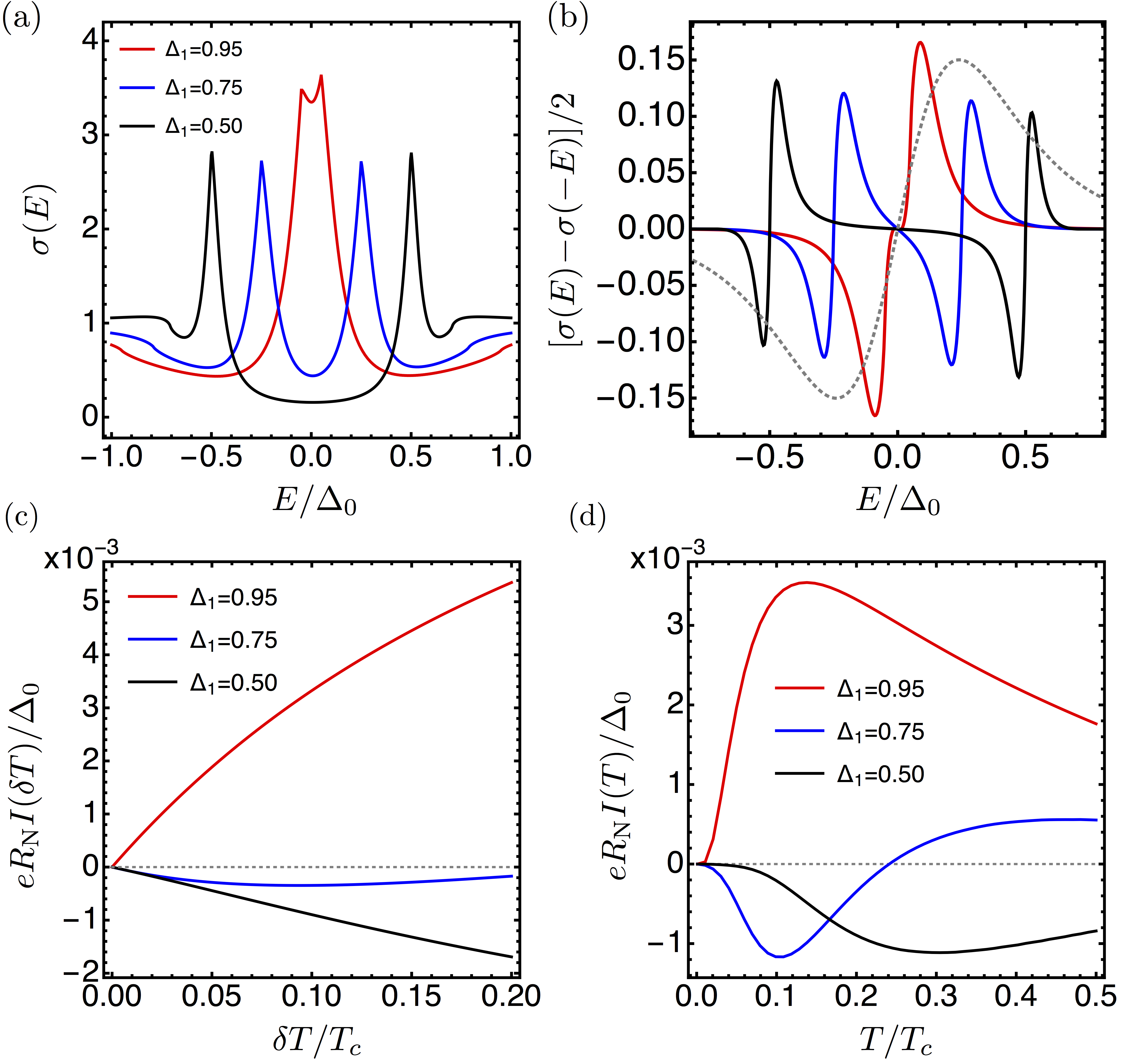
Figure 3: Conductance (a), its antisymmetric part (b), and the thermoelectric current (c,d) for a two-dimensional junction with $d_{xy}+is$-wave pairing. The dotted line in (b) is the difference in Fermi distribution functions for $T\!=\!0.2T_{\text{c}}$ and $\delta T\!=\!0.2T_{\text{c}}$. (c,d) Thermoelectric current as a function of the temperature bias for $T\!=\!0.2T_{c}$ (c) and the base temperature with $\delta T\!=\!T/2$ (d). In all cases, we have used $X=0.5$, $Z_{0}=3$ and $Z_{m}=0$.

III Andreev thermoelectric effect

To illustrate the effect of SABS on the thermoelectric current we start by considering a singlet $(d_{xy}+is)$-wave pairing,

$$\hat{\Delta}_{d+is}(\theta)=\Delta_{\text{T}}\left[\Delta_{1}\sin(2\theta)+i\Delta_{2}\right]i\hat{\sigma}_{2},$$ (17)

with $\Delta_{1}+\Delta_{2}=1$. Henceforth, the pairing temperature dependence is included in the amplitude by the interpolation formula $\Delta_{\text{T}}/\Delta_{0}\!=\!\tanh(1.74\sqrt{T_{c}/T-1})$. This pair potential was proposed as a fragile state Kashiwaya et al. (2004); Chesca et al. (2008) that could explain the splitting of the zero-bias peak in high-$T_{c}$ superconductors Biswas et al. (2002). We choose it because the parameter $\Delta_{1}\!=\!1-\Delta_{2}$ controls the evolution from a gap profile ($s$-wave, $\Delta_{1}\!=\!0$) into a zero-energy state ($d_{xy}$-wave, $\Delta_{1}\!=\!1$). The tunnel spectroscopy of the $(d_{xy}+is)$-wave state, Fig. 3(a), reveals that the zero-energy peak in the conductance from the $d_{xy}$-wave pairing splits in the presence of a small $s$-wave component until the Andreev resonances reach the gap edges at $E=\pm\Delta_{0}$, when $\Delta_{1}=0$.

The splitting of the zero-bias peak becomes asymmetric with the energy for an F-I-S junction with $X\!\neq\!0$. The energy-antisymmetric part of the resulting conductance, $[\sigma(E)-\sigma(-E)]/2$ in Fig. 3(b), presents a Fano-like sign change at the resonance positions. While well-separated resonances feature two Fano-like line shapes, one for positive and another for negative energies, there is only one Fano-like resonance when the SABS merge around zero energy ($\Delta_{1}\!\lesssim\!1$). This different behavior for separated and merged resonances explains the sign change in the current, Fig. 3(c,d). For a merged resonance, the anti-symmetric contribution to the conductance around zero energy follows the same profile as the difference in Fermi distributions $\delta f$ [indicated by a gray dotted line in Fig. 3(b)]. Consequently, the thermoelectric current is positive after integrating over the energy. By contrast, for separated resonances located at $E=\pm\delta E$, with $\delta E>0$, the anti-symmetric part of the conductance has the opposite sign to $\delta f$ in the energy range $|E|<\delta E$. For experimentally relevant temperatures Kolenda et al. (2016, 2017), $T\lesssim T_{c}/2$ and $\delta T\lesssim 0.3T_{c}$, this energy window provides the biggest contribution to the integral, and the resulting current is thus negative, see Fig. 3(c,d). The transition between these two regimes depends on the energy splitting between the SABS, with $\delta E\gtrsim\Delta_{0}/4$ enough to avoid a temperature-induced sign change.

We stress here that the asymmetry in the conductance only occurs at subgap energies, where the normal and Andreev probabilities for each spin channel, $B_{\sigma}=|b_{\sigma}|^{2}$ and $A_{\sigma}=\lambda_{\sigma}|a_{\sigma}|^{2}$, respectively, cf. Eq. 11, fulfill $B_{\sigma}=1-A_{\sigma}$. Consequently, the conductance is only due to Andreev processes, i.e., $\sigma=2R_{\text{N}}\langle P_{\uparrow}A_{\uparrow}+P_{\downarrow}A_{\downarrow}\rangle_{\mathbf{k}_{\parallel}}$, and the resulting thermoelectric current in Section II is Andreev-dominated, that is,

$$I(\delta T,V=0)=2I_{\text{A}}(\delta T,V=0).$$ (18)

We have thus demonstrated the Andreev thermoelectric effect for an F-I-S junction with $X\neq 0$ and $(d_{xy}+is)$-wave pairing and how the current goes from positive to negative in the presence or absence, respectively, of low-energy SABS. Within our approach, the necessary and sufficient condition for the Andreev thermoelectric effect is to break time-reversal and particle-hole symmetries per spin species so that the tunnel conductance becomes asymmetric with respect to the energy, cf. Eq. 16. This can be achieved for any pairing state in an F-I-S junction with $X\neq 0$, as a result of the different polarization of each spin channel shown in Eq. 12.

Spin	wave	$\hat{\Delta}(\theta_{\pm})$	SABS
Singlet	$s$	$\Delta_{\text{T}}i\hat{\sigma}_{2}$	$\times$
Triplet	$p$	$(\pm\Delta_{1}\cos\theta+i\Delta_{2}\sin\theta)\Delta_{\text{T}}\hat{\sigma}_{1}$	$\Delta_{1}\neq 0$
Singlet	$d$	$(\Delta_{1}\cos 2\theta\pm i\Delta_{2}\sin 2\theta)\Delta_{\text{T}}i\hat{\sigma}_{2}$	$\Delta_{2}\neq 0$

Table 1: Pairing potentials indicating the spin state, angular dependence and the condition for the emergence of SABS.

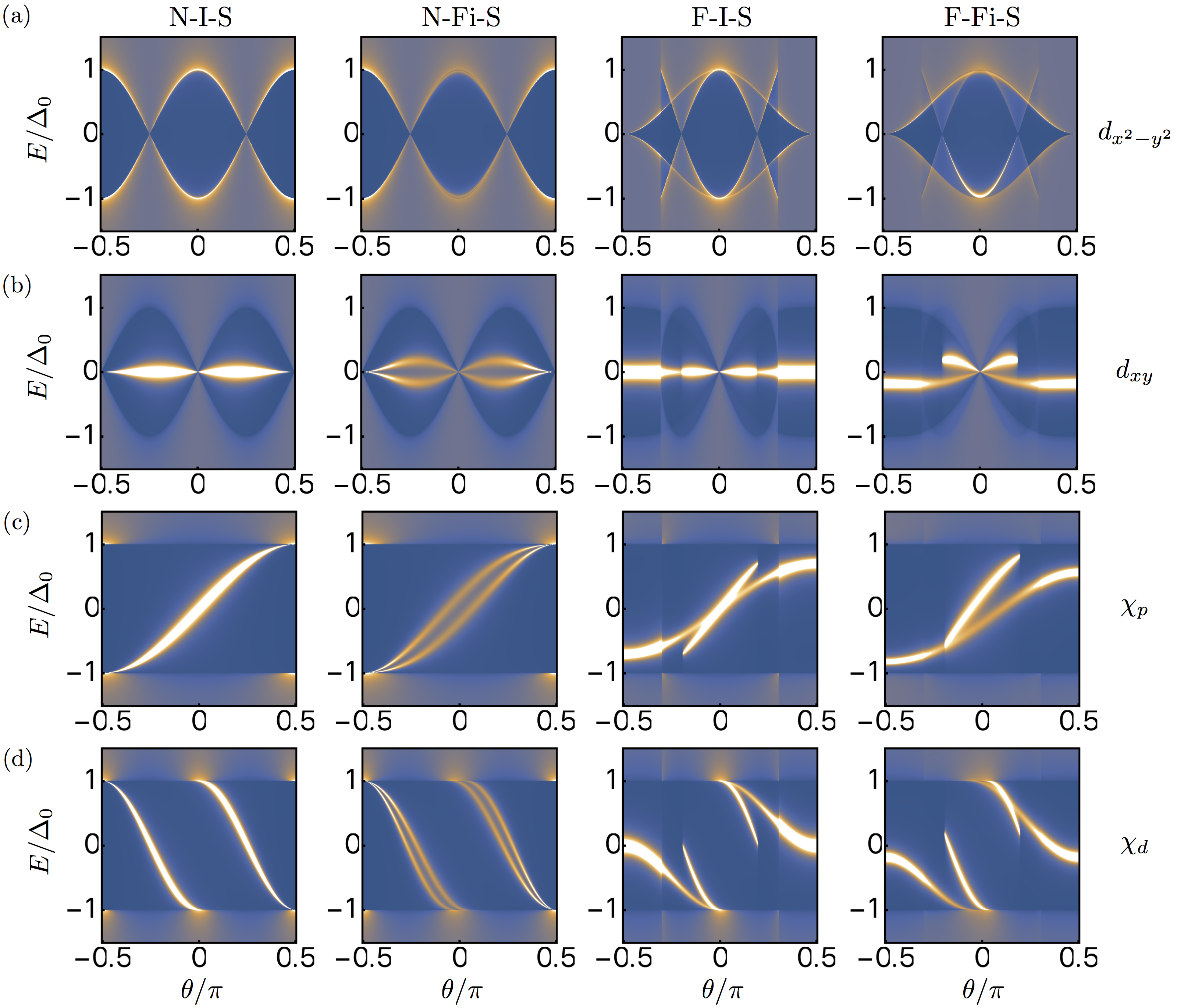
Figure 4: Spectral differential conductance $(\sum_{\sigma}P_{\sigma}\sigma_{\sigma}/\sigma_{\text{N}})$, where bright colors represent large conductances, for different junctions with the two-dimensional pair potentials (a) $d_{x^{2}-y^{2}}$-wave, (b) $d_{xy}$-wave (c) chiral $p$-wave ($\chi_{p}$) and (d) chiral $d$-wave ($\chi_{d}$). N-I-S and N-Fi-S (F-I-S and F-Fi-S) junctions have $X\!=\!0$ ($X\!=\!0.5$) and $Z_{m}=0$ and $Z_{m}=2.5$, respectively. We set $Z_{0}\!=\!5$ in all cases.

Indeed, the Andreev thermoelectric effect can occur in well-known unconventional superconductors. The $(d+is)$-wave pairing of our example explains a specific state of high-$T_{c}$ superconductors, which, more generally, feature an anisotropic $d$-wave singlet pair potential Kashiwaya and Tanaka (2000); [Forsimplicity; wedonotconsiderheremixedsinglet-tripletstatesthatcouldarisefrommagneticfluctuations; ]Kontani_2020. Spin-triplet $p$-wave states have been suggested as an explanation of the properties of UPt₃, Sr₂RuO₄ and other Ru-based compounds Mackenzie and Maeno (2003); Maeno et al. (2012); Kallin (2012). Some of these materials can develop topological phases, with the emergence of chiral states Kallin (2012). Most of these cases can be described by the pairing potentials listed in Table 1. Some three-dimensional (3D) chiral superconductors feature more complicated potentials that we detail later. In this section, we assume that the pairing rotational symmetry is preserved at the junction interface. We also define the effective pairing potentials for the right-moving electron- and hole-like quasiparticles in the superconducting region as $\Delta_{\sigma}^{+}$ and $\Delta_{\sigma}^{-}$, respectively, see Fig. 2(a). Rotational symmetry guarantees that $|\Delta_{\sigma}^{+}|=|\Delta_{\sigma}^{-}|$, and transmitted quasiparticles with the same spin thus experience the same pairing.

The spectral differential conductance, Fig. 4, illustrates the effect of the exchange fields on the subgap Andreev states for the four types of junctions considered here. For a tunnel N-I-S junction, it reveals the dispersion of the superconducting pairing. For example, $d_{x^{2}-y^{2}}$-wave features a nodal gap without SABS, while $d_{xy}$-wave presents the same anisotropy but displays zero-energy states, cf. Fig. 4(a,b). The chiral $p$- and $d$-wave states, Fig. 4(c) and Fig. 4(d), respectively, have SABS with linear dispersions, but only the chiral $p$-wave state crosses the zero energy point at zero momentum. In all cases, a ferromagnetic insulating barrier (N-Fi-S junction) causes a spin-splitting of the spectrum, very weak for the gapped $d_{x^{2}-y^{2}}$-wave case, but pronounced if SABS are present. The splitting, however, does not cause any asymmetry. Consequently, there is no current flowing from a temperature bias in an N-Fi-S junction.

A spin-active barrier alone is not enough to generate a thermoelectric effect; breaking time-reversal and particle-hole symmetries per spin species requires at least an F-I-S junction. When $X\!\neq\!0$, the angle of incidence $\theta$ for each spin channel becomes different, see Fig. 2(b). The maps in Fig. 4 show the superposed contribution of both channels, Eq. 11, revealing a strong angular asymmetry. In F-Fi-S junctions, the spin-active barrier further splits the spin bands, which, in addition to the angular asymmetry, greatly affects the thermoelectric current. If the spin-active barrier favors the majority spin species, in our case when $Z_{m}\!>\!0$ if $X\!>\!0$, the asymmetry at subgap energies is enhanced for all pairings, see Fig. 4. The resulting current is enhanced by an order of magnitude. Otherwise, when $Z_{m}\!<\!0$ for $X\!>\!0$, the current flow is reversed, see Fig. 5. The resulting thermoelectric currents still have opposite signs for gapped pairings and those featuring SABS, but their magnitude is smaller than for the case with parallel exchange fields. Notice that the crossover point takes place at $Z_{m}<0$, since there is a finite current at $Z_{m}=0$, cf. Fig. 5(a).

Fig. 5 shows how the sign of the thermoelectric current is positive (negative) for superconducting pairings featuring low-energy SABS (gap) in the conductance. To explain the direction of the current flow for the chiral $p$- or $d$-wave pairings, we need to take into account that, for a given angle $\theta$, the SABS can be located at any subgap energy, see Fig. 4(c,d). After the angle-average, however, the biggest contributions come from the angles around normal incidence ($\theta\!\sim\!0$). Therefore, the chiral $p$-wave pairing follows the behavior of a merged resonance, with a positive current, while the chiral $d$-wave case behaves like a separated one and thus provides a negative current. This different behavior of the chiral states is not always captured by the tunneling conductance, especially for 3d chiral superconductors Tamura et al. (2017).

Figure 5: Thermoelectric effect for the two-dimensional pair potentials listed in Table 1. (a) F-I-S junction with $Z_{m}=0$. (b) F-Fi-S junction with $X=0.5$. In all cases, $Z_{0}=3$, $T=0.2T_{\text{c}}$, and $\delta T=0.2T_{\text{c}}$.

The sign of the Andreev thermoelectric current thus pinpoints the presence or absence of low-energy Andreev states. If the SABS are exactly at zero energy, like for $p_{x}$- and $d_{xy}$-wave cases, the positive current is usually one or two orders of magnitude stronger than the negative one for gapped pairings, see Fig. 4. We note here that the negative current for gapped superconductors is already much larger than the expected thermoelectric current for equivalent, non-superconducting junctions Kalenkov et al. (2012); Ozaeta et al. (2014); Machon et al. (2014).

IV Odd-frequency pairing

We now show how a finite thermoelectric current is only possible if even and odd-frequency Cooper pairs coexist with similar amplitude. The Andreev reflection amplitude is related to the proximity-induced pairing, which can be described by the anomalous part of the Green’s function associated to Eq. 3. Following Refs. McMillan (1968); Furusaki and Tsukada (1991); Tanaka and Kashiwaya (1996b); Kashiwaya and Tanaka (2000); Asano (2001); Herrera et al. (2010); Crépin et al. (2015); Burset et al. (2015); Kashuba et al. (2017); Cayao and Black-Schaffer (2017, 2018); Lu and Tanaka (2018); Cayao et al. (2020) (see all the details in the appendix), we can write the anomalous Green’s function as

$$\hat{G}^{r}_{he}(x,x^{\prime};E,\theta_{S})=(f_{0}\hat{\sigma}_{0}-f_{3}\hat{\sigma}_{3})(i\hat{\sigma}_{2}),$$ (19)

where we have identified the spin-symmetric singlet and triplet components $f_{0}$ and $f_{3}$, respectively, as

$$f_{0,3}^{r}(0,0;E,\theta_{S})=\frac{a_{S,T}}{i\hbar}=\frac{a_{1\uparrow}(E,\theta_{S})}{i2\hbar v_{\uparrow}}\mp\frac{a_{1\downarrow}(E,\theta_{S})}{i2\hbar v_{\downarrow}}.$$ (20)

Here, $a_{S,T}$ are the singlet and triplet Andreev reflection amplitudes ($a_{1\sigma}$ corresponds to an injected electron in spin channel $\sigma$) and we have approximated the wave vectors as $k^{\sigma}_{e,h}\!\approx\!k_{\sigma}\pm E/(\hbar v_{\sigma})$, with $k_{\sigma}\!=\!k_{\text{F}}\sqrt{\cos^{2}\theta_{S}+\rho X}$ and $v_{\sigma}\!=\!\hbar k_{\sigma}/m$. It simplifies the symmetry analysis to use as reference the angle in the superconductor, $\theta_{S}$, which is the same for both spin channels, and only consider the anomalous Green’s function evaluated at the interface, where $x=x^{\prime}=0$.

Next, we define the even and odd parity parts of the anomalous functions as $f_{\mu,\pm}^{r}(E)\!=\![f_{\mu}^{r}(x,x^{\prime},E,\theta_{S})\pm f_{\mu}^{r}(x^{\prime},x,E,-\theta_{S})]/2$, with $\mu=0,3$ and the sign change in the angle due to the exchange $y\leftrightarrow y^{\prime}$. Then, to study the frequency dependence of the anomalous function, we use the retarded and advanced functions for positive and negative frequencies, respectively Burset et al. (2015), since only there these functions have physical meaning. Consequently, the anomalous function

$$f(x,x^{\prime};E,\theta_{S})=\left\{\begin{array}[]{cr}f^{r}(x,x^{\prime};E,\theta_{S}),&E>0\\ f^{a}(x,x^{\prime};E,\theta_{S}),&E<0\end{array}\right.$$ (21)

connects both energy branches. Once the anomalous function in Eq. 21 is fully symmetric with respect to spin and parity, it belongs to one of four possible symmetry classes. We label the different classes by their spin state, S for singlet and T for triplet, and their symmetry, even (E) or odd (O), with respect to frequency and space coordinates. For example, even-frequency, singlet, even-parity is ESE and ETO refers to the even-frequency, triplet odd-parity case Tanaka and Golubov (2007); Tanaka et al. (2007a, b, 2012).

It is now useful to define the short-hand notation $a^{\alpha}_{\beta}=(\alpha E,\beta\theta)$, with $\alpha,\beta=\pm$ and $a$ standing for either of $a_{S,T}$, and thus write the energy- and angle-symmetric parts of the amplitude $a$ as

$$a^{Ee,Eo}={} \frac{1}{4}\left(a^{+}_{+}+a^{-}_{+}\pm a^{+}_{-}\pm a^{-}_{-}\right),$$ (22a)

$$a^{Oe,Oo}={} \frac{1}{4}\left(a^{+}_{+}-a^{-}_{+}\pm a^{+}_{-}\mp a^{-}_{-}\right).$$ (22b)

Here, the index $a^{E,O}$ ($a^{e,o}$) labels the even and odd parts of the amplitude with respect to the energy (angle). From the particle-hole symmetry of the Hamiltonian in Eq. 3 and the micro-reversibility of the scattering matrix, we obtain the condition $v_{\downarrow,\uparrow}a_{1\uparrow,\downarrow}(E,\theta)=-v_{\uparrow,\downarrow}a^{*}_{1\downarrow,\uparrow}(-E,-\theta)$ for $|\theta_{S}|\leq\theta_{c}\!=\!\sin^{-1}\sqrt{1-X}$, see the appendix for more details. Once applied to the singlet and triplet amplitudes, this condition reads $a_{S,T}(E,\theta)=\pm a_{S,T}^{*}(-E,-\theta)$, and combined with Eq. 22 reveals that, in the absence of virtual Andreev processes ($|\theta_{S}|\leq\theta_{c}$), the amplitudes $a_{S}^{Ee}$, $a_{S}^{Oo}$, $a_{T}^{Eo}$ and $a_{T}^{Oe}$ are real, while the rest are purely imaginary. Therefore, at the interface we find

$$f_{\text{ESE}}={} \left\{\begin{array}[]{rclr}-\frac{i}{2\hbar}(a_{S}^{Ee}+i\bar{a}_{S}^{Oe}),&E>0\\ -\frac{i}{2\hbar}(a_{S}^{Ee}+i\bar{a}_{S}^{Oe}),&E<0\end{array}\right.,$$ (23c)

$$f_{\text{OSO}}={} \left\{\begin{array}[]{rclr}-\frac{i}{2\hbar}(a_{S}^{Oo}+i\bar{a}_{S}^{Eo}),&E>0\\ +\frac{i}{2\hbar}(a_{S}^{Oo}+i\bar{a}_{S}^{Eo}),&E<0\end{array}\right.,$$ (23f)

$$f_{\text{ETO}}={} \left\{\begin{array}[]{rclr}-\frac{i}{2\hbar}(a_{T}^{Eo}+i\bar{a}_{T}^{Oo}),&E>0\\ -\frac{i}{2\hbar}(a_{T}^{Eo}+i\bar{a}_{T}^{Oo}),&E<0\end{array}\right.,$$ (23i)

$$f_{\text{OTE}}={} \left\{\begin{array}[]{rclr}-\frac{i}{2\hbar}(a_{T}^{Oe}+i\bar{a}_{T}^{Ee}),&E>0\\ +\frac{i}{2\hbar}(a_{T}^{Oe}+i\bar{a}_{T}^{Ee}),&E<0\end{array}\right.,$$ (23l)

where we substituted the purely imaginary amplitudes as $a=i\bar{a}$, with $\bar{a}$ being real. It is then straightforward to check that $f_{\text{ESE}}$ and $f_{\text{OSO}}$ in Eq. 23 are, respectively, even and odd in both frequency and parity .

We can now establish a connection between the thermoelectric current and the symmetry of the pairing state. Focusing on the Andreev contribution to Eq. 16, which we have demonstrated to be equal to the total current, we find

$$I_{\text{A}}=\frac{1}{eR_{\text{N}}}\int_{0}^{\infty}\!dE\,\delta f$$

$$\times\langle v_{\uparrow}v_{\downarrow}\left[|a_{S}(E)|^{2}-|a_{S}(-E)|^{2}+|a_{T}(E)|^{2}-|a_{T}(-E)|^{2}\right.$$

$$\left.+2X\mathrm{Re}\left\{a_{S}(E)a_{T}^{*}(E)-a_{S}(-E)a_{T}^{*}(-E)\right\}\right]\rangle_{\mathbf{k}_{\parallel}},$$ (24)

where we have used that $\lambda_{\sigma}=v_{\bar{\sigma}}/v_{\sigma}$. It is clear from Eq. 24 that a finite polarization ($X\!\neq\!0$) couples the spin singlet and triplet states, resulting in a new contribution to the current. To identify the scattering amplitudes with the anomalous Green’s function, we first note that the virtual Andreev processes do not contribute to the current and thus the angle average is limited to $|\theta_{S}|\!\leq\!\theta_{c}$. Then, using Eqs. 22 and 23 we can write the scattering amplitudes in the absence of virtual processes as

$$a_{S}(E)={} 2i\hbar f_{\text{ESE}}+2i\hbar f_{\text{OSO}},$$ (25a)

$$a_{S}(-E)={} 2i\hbar\left(f_{\text{ESE}}\right)^{*}-2i\hbar\left(f_{\text{OSO}}\right)^{*},$$ (25b)

$$a_{T}(E)={} 2i\hbar f_{\text{OTE}}+2i\hbar f_{\text{ETO}},$$ (25c)

$$a_{T}(-E)={} 2i\hbar\left(f_{\text{ETO}}\right)^{*}-2i\hbar\left(f_{\text{OTE}}\right)^{*}.$$ (25d)

Inserting Eqs. (25) into Eq. 24, the current becomes

$$I_{\text{A}}=\frac{16\hbar^{2}}{eR_{\text{N}}}\int_{0}^{\infty}\!dE\,\delta f$$

$$\times\mathrm{Re}\left\{\langle v_{\uparrow}v_{\downarrow}\left[\left(f_{\text{ESE}}\right)^{*}f_{\text{OSO}}+\left(f_{\text{ETO}}\right)^{*}f_{\text{OTE}}\right]\right.$$

$$\left.+v_{\uparrow}v_{\downarrow}X\left[\left(f_{\text{ESE}}\right)^{*}f_{\text{OTE}}+\left(f_{\text{ETO}}\right)^{*}f_{\text{OSO}}\right]\rangle_{\mathbf{k}_{\parallel}}\right\}.$$ (26)

In general, the angle-average of the product of functions of opposite parity in the same spin state is zero, i.e., $\langle f_{\text{ESE}}^{*}f_{\text{OSO}}\rangle_{\mathbf{k}_{\parallel}}=\langle f_{\text{ETO}}^{*}f_{\text{OTE}}\rangle_{\mathbf{k}_{\parallel}}=0$. Consequently, there is no thermoelectric current in N-I-S junctions, with $X=0$, even though a strong odd-frequency pairing appears in the presence of SABS Tanaka et al. (2012). By contrast, in F-I-S junctions for arbitrary pairings, see Fig. 5, the thermoelectric effect is then due to the term proportional to $X$, which mixes even- and odd-frequency terms with different spin states . Therefore, the Andreev thermoelectric effect is only possible if even and odd-frequency pairing coexist Hwang et al. (2018).

Figure 6: Thermoelectric current as a function of the misalignment angle $\alpha$ in an F-I-S junction. (a) Two-dimensional ($d_{xy}+is$)-wave pairing for different values of $\Delta_{1}$. (b) 3D chiral pairing in Eq. 27 for $\nu=1,2$. Top panels show the relative orientation between the pairing potential and the interface. The insets show the quasiparticle contribution to the current. In all cases we set $X=0.5$, $Z_{0}=3$, $Z_{m}\!=\!0$, $T=0.1T_{\text{c}}$, and $\delta T=0.2T_{\text{c}}$.

V Broken rotational symmetry

In all the previous results, the Andreev thermoelectric effect is due to subgap processes where only Cooper pairs are transmitted into the superconductor, see Eq. 18, for any value of $X$ or $Z_{m}$. However, the transport properties of unconventional anisotropic pairings depend strongly on the relative orientation between the pairing potential and the junction interface. For example, for $d_{xy}$-wave pairing, the effective pairings for electron- and hole-like quasiparticles are $\Delta_{\sigma}^{\pm}=\pm\rho\Delta_{0}\sin\left(2\theta-2\alpha\right)$, respectively, where $\alpha$ is the misalignment angle Tanaka and Kashiwaya (1995); Kashiwaya et al. (1996). When $\alpha$ is different from one of the highly symmetric orientations, $\alpha\neq 0,\pi/4$, the rotational symmetry for $d_{xy}$-wave is broken and $|\Delta_{\sigma}^{+}|\neq|\Delta_{\sigma}^{-}|$, resulting in a small contribution to the thermoelectric current from quasiparticles.

We show the effect of the misalignment angle in an F-I-S junction with $d_{xy}+is$-wave pairing in Fig. 6(a). When $\alpha\neq 0,\pi/4$, the transport properties change. For normalized energies $E/\Delta_{0}$ below $\Delta_{2}=1-\Delta_{1}$, the system is fully gapped, the condition $\sigma=2R_{\text{N}}\langle P_{\uparrow}A_{\uparrow}+P_{\downarrow}A_{\downarrow}\rangle_{\mathbf{k}_{\parallel}}$ holds and the antisymmetric part of the conductance is only due to Andreev processes. However, for $\Delta_{2}<|E/\Delta_{0}|<1$ quasiparticles can be transferred into the superconductor. Consequently, the subgap condition $A_{\sigma}+B_{\sigma}=1$ no longer holds and the quasiparticle term $I_{\text{qp}}$ becomes finite in Section II. Even though the current now has two contributions, $I_{\text{A}}$ and $I_{\text{qp}}$, we are clearly in the situation where $I_{\text{A}}>I_{\text{qp}}$, see inset of Fig. 6(a). For the two-dimensional pairings considered here, the quasiparticle current generated by a broken rotational symmetry is not enough to change the sign of the total current around the highly symmetric orientations.

The results from the previous section can be extended to 3D unconventional superconductors without loss of generality. In higher dimensions, however, the energy dispersion of SABS can become more complicated Murakawa et al. (2009); Sasaki et al. (2011). Recently, the exotic SABS of 3d chiral superconductors have attracted a lot of attention due to the simultaneous presence of line and point nodes Asano et al. (2003); Qi et al. (2009); Chung and Zhang (2009); Fu and Berg (2010); Hao and Lee (2011); Hsieh and Fu (2012); Yamakage et al. (2012); Hashimoto et al. (2015); Lu et al. (2015); Hashimoto et al. (2016). The SABS of 3d chiral superconductors are predicted to originate from the pair potential

$$\hat{\Delta}^{\nu}_{3\text{d}}(\mathbf{k})=\Delta_{\text{T}}\frac{k^{\prime}_{x}\left(k_{y}+ik^{\prime}_{z}\right)^{\nu}}{r_{\nu}k_{\text{F}}^{\nu+1}}\times\left\{\begin{array}[]{cl}i\hat{\sigma}_{2},&\nu\text{ odd}\\ \hat{\sigma}_{1},&\nu\text{ even}\end{array}\right.,$$ (27)

with $k^{\prime}_{x}=k_{x}\cos\alpha-k_{z}\sin\alpha$, $k^{\prime}_{z}=k_{x}\sin\alpha+k_{z}\cos\alpha$, $\alpha$ being the misalignment angle from the $k_{x}$ axis, $\nu$ a nonzero integer Kobayashi et al. (2015); Tamura et al. (2017), and the normalization factors $(r_{\nu=0},r_{\nu=1},r_{\nu=2})=(1,1/2,2/\sqrt{27})$. For $\nu=0$, the potential features a line node, while it has two point nodes and a line node for $\nu=1,2$. The pairing is in a spin-triplet (singlet) state for $\nu$ even (odd).

While the case with $\nu=0$ generalizes the two-dimensional chiral $p$-wave triplet pairing of the previous section, the cases with finite $\nu$ are relevant for heavy fermion superconductors, with $\nu=1$ and $\nu=2$ corresponding to the candidate pairing symmetries of URu₂Si₂ Kasahara et al. (2007); Shibauchi et al. (2014); Schemm et al. (2015) and UPt₃ Joynt and Taillefer (2002); Tsutsumi et al. (2012, 2013); Schemm et al. (2014); Goswami and Nevidomskyy (2015), respectively. The topological origin of the flat-band SABS and its fragility against surface misalignment have been clarified in previous works Kobayashi et al. (2015), together with the SABS energy dispersion Tamura et al. (2017). It was found that a unique characteristic of the $\nu\!=\!1,2$ pairings is that an external exchange field can turn a zero-bias conductance peak into a dip, due to the complicated dispersion of the SABS Tamura et al. (2017). Consequently, an equivalent sign change in the thermoelectric current appears here.

The thermoelectric current for 3d chiral superconductors behaves like the two-dimensional cases for highly symmetric orientations ($\alpha=0,\pi/2$). For different surface misalignments, however, the quasiparticle contribution from broken rotational symmetry can affect the sign of the current, see Fig. 6(b). In the presence of a zero-energy SABS, however, the quasiparticle contribution is smaller than the Andreev one and the current remains positive. The sign change of the thermoelectric current thus clearly indicates the presence of SABS, even when they have a complicated energy dispersion. Moreover, some orientations, like $\alpha=\pi/2$, have a very different zero-energy behavior depending on the value of $\nu$. For $\nu=1$ and $\nu=2$, the pairing can be regarded as a chiral $p$-wave or chiral $d$-wave, which feature the opposite signs of the current. Consequently, the sign of the thermoelectric current is, again, a good indicator of the presence of SABS, even if the surface states display a complicated dispersion relation.

VI Summary

Following a microscopic scattering approach, we have shown that the thermoelectric effect in ferromagnet-superconductor junctions can be entirely dominated by subgap Andreev processes. Consequently, the electric current from a temperature bias changes sign in the presence of SABS from unconventional superconductivity and is thus a sensitive tool to identify these surface states.

When the rotational symmetry of the pairing potential is maintained at the junction interface (that is, $|\Delta_{\sigma}^{+}|=|\Delta_{\sigma}^{-}|$ for each spin channel $\sigma$) the transport asymmetry that gives rise to the thermoelectric effect occurs only at subgap energies. The resulting current is dominated by Andreev processes, $I(\delta T)=2I_{\text{A}}(\delta T)$, with no quasiparticle transfer into the superconductor. A finite polarization induced by a Zeeman exchange field $X$ in an F-I-S junction is a necessary and sufficient condition for this Andreev thermoelectric effect. An additional intermediate ferromagnetic insulator, F-Fi-S junction, enhances the magnitude of the current if the majority spin species is favored (i.e., $Z_{m}>0$ for $X>0$). We have shown how the exchange field allows for the coupling of even- and odd-frequency Cooper pairs leaking out of the superconductor, which provide the main contribution to the Andreev thermoelectric current. Thermoelectric measurements in F-I-S setups can thus complement recent experimental signatures of odd-frequency pairing Perrin et al. (2020); *Simon_2020b.

For F-Fi-S junctions, we restricted our analysis to the case of collinear exchange fields in the ferromagnet and ferromagnetic insulator. For non-collinear fields, a long-range, odd-frequency triplet state emerges Bergeret et al. (2001); *Bergeret_RMP; Khaire et al. (2010); Robinson et al. (2010a, b), which could enhance the thermoelectric current according to Eq. 26 Dutta et al. (2017, 2020). In particular, Ref. [Dutta et al., 2020] shows that a large figure of merit is possible for F-Fi-S junctions with non-collinear exchange fields and conventional superconductors.

When the pairing rotational symmetry is broken ($|\Delta_{\sigma}^{+}|\!\neq\!|\Delta_{\sigma}^{-}|$), quasiparticle transfers into the superconductor are allowed and contribute to the thermoelectric current. Such contributions could change the sign of the current and mask the presence of SABS. However, we have analyzed the thermoelectric effect for two- and three-dimensional pairings with a strong angular dependence and when low-energy SABS are present the current is positive, Andreev-dominated and with a strong magnitude around highly-symmetric orientations. As such, the sign of the thermoelectric current could help identify the pairing state even for cases where the outcome of tunneling spectroscopy can be ambiguous.

In conclusion, exploring the thermoelectric effect in ferromagnet-superconductor hybrid junctions involving unconventional superconductors offers a sensitive method to identify emerging surface Andreev states. Our results can be easily extended to heterostructures where topological superconductivity is artificially engineered by combining conventional superconductors with topological materials Jäck et al. (2019).

Appendix A Retarded Green’s function

Following Refs. McMillan (1968); Furusaki and Tsukada (1991); Tanaka and Kashiwaya (1996b); Kashiwaya and Tanaka (2000); Asano (2001); Herrera et al. (2010); Crépin et al. (2015); Burset et al. (2015); Kashuba et al. (2017); Cayao and Black-Schaffer (2017, 2018); Lu and Tanaka (2018); Cayao et al. (2020), the retarded Green’s function associated with the Hamiltonian in Eq. 3 is constructed from a linear combination of scattering states obtained from Eq. 7 with the appropriate boundary conditions. We now describe the main steps of this method for a generic pairing potential.

First, since the spin channels in Eq. 3 are decoupled, we only need to work with the reduced Hamiltonian

$$\hat{H}_{\sigma}(x,\mathbf{k})=\left(\begin{array}[]{cc}h_{\sigma}(x)-\mu&\Delta_{\sigma}(\mathbf{k}_{\parallel}/k_{\text{F}})\mathrm{e}^{i\phi}\\ \Delta^{*}_{\sigma}(\mathbf{k}_{\parallel}/k_{\text{F}})\mathrm{e}^{-i\phi}&\mu-h_{\sigma}(x)\end{array}\right),$$ (28)

where

$$h_{\sigma}(x)=-\frac{\hbar^{2}}{2m}\frac{d^{2}}{dx^{2}}-\rho U(x)+\left(V_{0}-\rho U_{\text{B}}\right)\delta(x).$$ (29)

The retarded Green’s function thus satisfies the equation of motion

$$\delta(x-x^{\prime})=\left[\hat{E}_{+}-\hat{H}_{\sigma}(x,\mathbf{k})\right]\hat{G}^{r}_{\sigma}(x,x^{\prime};E,\mathbf{k}_{\parallel})=\hat{G}^{r}_{\sigma}(x,x^{\prime};E,\mathbf{k}_{\parallel})\left[\hat{E}_{+}-\hat{H}^{T}_{\sigma}(x,\mathbf{k})\right],$$ (30)

with $\hat{E}_{+}=(E+i0^{+})\hat{\sigma}_{0}$, which can be integrated to obtain the following boundary conditions:

$$0={} \hat{G}^{r}_{\sigma}(x,x+0^{+})-\hat{G}^{r}_{\sigma}(x,x-0^{+}),$$ (31a)

$$\frac{2m}{\hbar^{2}}\hat{\tau}_{3}={} \left.\partial_{x}\hat{G}^{r}_{\sigma}(x,x^{\prime})\right|_{x=x^{\prime}+0^{+}}-\left.\partial_{x}\hat{G}^{r}_{\sigma}(x,x^{\prime})\right|_{x=x^{\prime}-0^{+}}.$$ (31b)

A general solution of the BdG equations for $\hat{H}_{\sigma}(x,\mathbf{k})$ takes the form

$$\Phi_{\sigma}(\mathbf{r})=\mathrm{e}^{i(k_{y}y+k_{z}z)}\sum\limits_{\alpha=\pm}\left[m^{\alpha}_{\sigma}\psi_{\alpha k^{\sigma}_{1}}\mathrm{e}^{\alpha ik^{\sigma}_{1}x}+n^{\alpha}_{\sigma}\psi_{\alpha k^{\sigma}_{2}}\mathrm{e}^{\alpha ik^{\sigma}_{2}x}\right],$$

where $\psi_{\pm k^{\sigma}_{1}}=[1,(\eta^{\pm}_{\sigma})^{*}\Gamma^{\pm}_{\sigma}]^{T}$ ($\psi_{\pm k^{\sigma}_{2}}=[\eta^{\pm}_{\sigma}\Gamma^{\pm}_{\sigma},1]^{T}$) is the solution for an electron-like (hole-like) quasiparticle with amplitude $m^{\alpha}_{\sigma}$ ($n^{\alpha}_{\sigma}$), cf. Eq. 7. For the transposed Hamiltonian, we find

$$\tilde{\Phi}_{\sigma}(\mathbf{r})=\mathrm{e}^{-i(k_{y}y+k_{z}z)}\sum\limits_{\alpha=\pm}\left[\tilde{m}^{\alpha}_{\sigma}\tilde{\psi}_{\alpha k^{\sigma}_{1}}\mathrm{e}^{\alpha ik^{\sigma}_{1}x}+\tilde{n}^{\alpha}_{\sigma}\tilde{\psi}_{\alpha k^{\sigma}_{2}}\mathrm{e}^{\alpha ik^{\sigma}_{2}x}\right],$$

with $\tilde{\psi}_{\pm k^{\sigma}_{1}}=[1,\eta^{\mp}_{\sigma}\Gamma^{\mp}_{\sigma}]^{T}$ and $\tilde{\psi}_{\pm k^{\sigma}_{2}}=[(\eta^{\mp}_{\sigma})^{*}\Gamma^{\mp}_{\sigma},1]^{T}$. Notice that both the extra conjugation and the exchange $\theta_{+}\leftrightarrow\theta_{-}$ are a result of the transposition (we take the superconducting phase to be zero for the sake of simplicity). The four possible scattering states for an F-I-S junction are injection of electron (1) or hole (2) from the ferromagnet and injection of an electron- (3) or hole-like (4) quasiparticle from the superconductor. Specifically, we have

$$\phi_{\sigma,1}(x)={} \left\{\begin{array}[]{cr}\psi_{+k^{\sigma}_{e}}\mathrm{e}^{ik^{\sigma}_{e}x}+a^{\sigma}_{1}\psi_{+k^{\sigma}_{h}}\mathrm{e}^{ik^{\sigma}_{h}x}+b^{\sigma}_{1}\psi_{-k^{\sigma}_{e}}\mathrm{e}^{-ik^{\sigma}_{e}x},&x<0\\ c^{\sigma}_{1}\psi_{+k^{\sigma}_{1}}\mathrm{e}^{ik^{\sigma}_{1}x}+d^{\sigma}_{1}\psi_{-k^{\sigma}_{2}}\mathrm{e}^{-ik^{\sigma}_{2}x},&x>0\end{array}\right.,$$ (32c)

$$\phi_{\sigma,2}(x)={} \left\{\begin{array}[]{cr}\psi_{-k^{\sigma}_{h}}\mathrm{e}^{-ik^{\sigma}_{h}x}+b^{\sigma}_{2}\psi_{+k^{\sigma}_{h}}\mathrm{e}^{ik^{\sigma}_{h}x}+a^{\sigma}_{2}\psi_{-k^{\sigma}_{e}}\mathrm{e}^{-ik^{\sigma}_{e}x},&x<0\\ d^{\sigma}_{2}\psi_{+k^{\sigma}_{1}}\mathrm{e}^{ik^{\sigma}_{1}x}+c^{\sigma}_{2}\psi_{-k^{\sigma}_{2}}\mathrm{e}^{-ik^{\sigma}_{2}x},&x>0\end{array}\right.,$$ (32f)

$$\phi_{\sigma,3}(x)={} \left\{\begin{array}[]{cr}d^{\sigma}_{3}\psi_{+k^{\sigma}_{h}}\mathrm{e}^{ik^{\sigma}_{h}x}+c^{\sigma}_{3}\psi_{-k^{\sigma}_{e}}\mathrm{e}^{-ik^{\sigma}_{e}x},&x<0\\ \psi_{-k^{\sigma}_{1}}\mathrm{e}^{-ik^{\sigma}_{1}x}+b^{\sigma}_{3}\psi_{+k^{\sigma}_{1}}\mathrm{e}^{ik^{\sigma}_{1}x}+a^{\sigma}_{3}\psi_{-k^{\sigma}_{2}}\mathrm{e}^{-ik^{\sigma}_{2}x},&x>0\end{array}\right.,$$ (32i)

$$\phi_{\sigma,4}(x)={} \left\{\begin{array}[]{cr}c^{\sigma}_{4}\psi_{+k^{\sigma}_{h}}\mathrm{e}^{ik^{\sigma}_{h}x}+d^{\sigma}_{4}\psi_{-k^{\sigma}_{e}}\mathrm{e}^{-ik^{\sigma}_{e}x},&x<0\\ \psi_{k^{\sigma}_{2}}\mathrm{e}^{ik^{\sigma}_{1}x}+a^{\sigma}_{4}\psi_{+k^{\sigma}_{1}}\mathrm{e}^{ik^{\sigma}_{1}x}+b^{\sigma}_{4}\psi_{-k^{\sigma}_{2}}\mathrm{e}^{-ik^{\sigma}_{2}x},&x>0\end{array}\right.,$$ (32l)

where the wave vectors in the normal regions are $k^{\sigma}_{e,h}$ and thus $\psi_{\pm k^{\sigma}_{e}}\!=\!(1,0)^{T}$ and $\psi_{\pm k^{\sigma}_{h}}\!=\!(0,1)^{T}$, since $\eta^{\pm}_{\sigma}\!=\!0$. Finally, the retarded Green’s function is a linear combination of asymptotic solutions of $\hat{H}_{\sigma}(x,\mathbf{k})$ and $\hat{H}^{T}_{\sigma}(x,\mathbf{k})$, namely,

$$\hat{G}^{r}_{\sigma}(x,x^{\prime})=\left\{\begin{array}[]{lr}\phi_{\sigma,3}(x)\left[\alpha^{\sigma}_{1}\tilde{\phi}_{\sigma,1}^{T}(x^{\prime})+\alpha^{\sigma}_{3}\tilde{\phi}_{\sigma,2}^{T}(x^{\prime})\right]+\phi_{\sigma,4}(x)\left[\alpha^{\sigma}_{2}\tilde{\phi}_{\sigma,1}^{T}(x^{\prime})+\alpha^{\sigma}_{4}\tilde{\phi}_{\sigma,2}^{T}(x^{\prime})\right],&x<x^{\prime}\\ \phi_{\sigma,1}(x)\left[\beta^{\sigma}_{1}\tilde{\phi}_{\sigma,3}^{T}(x^{\prime})+\beta^{\sigma}_{3}\tilde{\phi}_{\sigma,4}^{T}(x^{\prime})\right]+\phi_{\sigma,2}(x)\left[\beta^{\sigma}_{2}\tilde{\phi}_{\sigma,3}^{T}(x^{\prime})+\beta^{\sigma}_{4}\tilde{\phi}_{\sigma,4}^{T}(x^{\prime})\right],&x>x^{\prime}\end{array}\right..$$ (33)

The coefficients of the linear combination are obtained by imposing the boundary conditions in Eq. 31. Focusing on the region with $x,x^{\prime}<0$, we find from the Nambu-diagonal elements the system of equations

$$d^{\sigma}_{3}\alpha^{\sigma}_{1}+c^{\sigma}_{4}\alpha^{\sigma}_{3}=\tilde{d}^{\sigma}_{3}\beta_{1}+\tilde{c}^{\sigma}_{4}\beta^{\sigma}_{3}=c^{\sigma}_{3}\alpha^{\sigma}_{2}+d^{\sigma}_{4}\alpha^{\sigma}_{4}=\tilde{c}^{\sigma}_{3}\beta_{2}+\tilde{d}^{\sigma}_{4}\beta^{\sigma}_{4}={} 0,$$ (34a)

$$c^{\sigma}_{3}\alpha^{\sigma}_{1}+d^{\sigma}_{4}\alpha^{\sigma}_{3}-\tilde{c}^{\sigma}_{3}\beta_{1}-\tilde{d}^{\sigma}_{4}\beta^{\sigma}_{3}=d^{\sigma}_{3}\alpha^{\sigma}_{2}+c^{\sigma}_{4}\alpha^{\sigma}_{4}-\tilde{d}^{\sigma}_{3}\beta_{2}-\tilde{c}^{\sigma}_{4}\beta^{\sigma}_{4}={} 0,$$ (34b)

$$c^{\sigma}_{3}\alpha^{\sigma}_{1}+d^{\sigma}_{4}\alpha^{\sigma}_{3}+\tilde{c}^{\sigma}_{3}\beta_{1}+\tilde{d}^{\sigma}_{4}\beta^{\sigma}_{3}={} \frac{2m}{i\hbar^{2}k^{\sigma}_{e}},$$ (34c)

$$d^{\sigma}_{3}\alpha^{\sigma}_{2}+c^{\sigma}_{4}\alpha^{\sigma}_{4}+\tilde{d}^{\sigma}_{3}\beta_{2}+\tilde{c}^{\sigma}_{4}\beta^{\sigma}_{4}={} \frac{2m}{i\hbar^{2}k^{\sigma}_{h}},$$ (34d)

resulting in

$$\alpha^{\sigma}_{1}={} -\frac{c^{\sigma}_{4}}{d^{\sigma}_{3}}\alpha^{\sigma}_{3}=\frac{-i}{\hbar v^{\sigma}_{e}}\frac{c^{\sigma}_{4}}{c^{\sigma}_{3}c^{\sigma}_{4}-d^{\sigma}_{3}d^{\sigma}_{4}},\quad\alpha^{\sigma}_{2}=-\frac{d^{\sigma}_{4}}{c^{\sigma}_{3}}\alpha^{\sigma}_{4}=\frac{i}{\hbar v^{\sigma}_{h}}\frac{d^{\sigma}_{4}}{c^{\sigma}_{3}c^{\sigma}_{4}-d^{\sigma}_{3}d^{\sigma}_{4}},$$ (35a)

$$\beta^{\sigma}_{1}={} -\frac{\tilde{c}^{\sigma}_{4}}{\tilde{d}^{\sigma}_{3}}\beta^{\sigma}_{3}=\frac{-i}{\hbar v^{\sigma}_{e}}\frac{\tilde{c}^{\sigma}_{4}}{\tilde{c}^{\sigma}_{3}\tilde{c}^{\sigma}_{4}-\tilde{d}^{\sigma}_{3}\tilde{d}^{\sigma}_{4}},\quad\beta^{\sigma}_{2}=-\frac{\tilde{d}^{\sigma}_{4}}{\tilde{c}^{\sigma}_{3}}\beta^{\sigma}_{4}=\frac{i}{\hbar v^{\sigma}_{h}}\frac{\tilde{d}^{\sigma}_{4}}{\tilde{d}^{\sigma}_{3}\tilde{d}^{\sigma}_{4}-\tilde{d}^{\sigma}_{3}\tilde{d}^{\sigma}_{4}},$$ (35b)

with $v^{\sigma}_{e,h}=\hbar k^{\sigma}_{e,h}/m$ being the velocity for spin $\sigma$ electrons and holes, respectively. On the other hand, the Nambu off-diagonal sector provides the detailed balance equations

$$k^{\sigma}_{h}\tilde{a}^{\sigma}_{1}=k^{\sigma}_{e}a^{\sigma}_{2},\quad k^{\sigma}_{h}a^{\sigma}_{1}=k^{\sigma}_{e}\tilde{a}^{\sigma}_{2},$$ (36)

which can be demonstrated using the Wronskian of the scattering processes 1 and 2. For Nambu spinors $\psi_{j}(x)\!=\![u_{j}(x),v_{j}(x)]^{T}$, the Wronskian is defined as

$$W\left[\psi_{i}(x),\psi_{j}(x)\right]\equiv u_{i}u^{\prime}_{j}-u_{j}u^{\prime}_{i}-\left(v_{i}v^{\prime}_{j}-v_{j}v^{\prime}_{i}\right),$$ (37)

with $u^{\prime}\!=\!du(x)/dx$. For the scattering processes 1 and 2, we obtain

$$W[\phi_{\sigma,1}(x),\tilde{\phi}_{\sigma,2}]=\left\{\begin{array}[]{cr}2i\left(k^{\sigma}_{h}a^{\sigma}_{1}-k^{\sigma}_{e}\tilde{a}^{\sigma}_{2}\right),&x<0\\ 0,&x>0\end{array}\right..$$ (38)

The Wronskian is independent of the coordinate $x$ and, thus, equating the two branches of the Wronskian, we obtain one of the detailed balance equations in Eq. 36. The other one comes from $W[\tilde{\phi}_{\sigma,1}(x),\phi_{\sigma,2}]$.

By plugging the linear coefficients in Eq. 35 into Eq. 33, and using the detailed balance relations in Eq. 36, we obtain the retarded Green’s function per spin channel in the normal region as

$$\hat{G}^{r}_{\sigma}(x,x^{\prime})=\frac{1}{i\hbar}\begin{pmatrix}\frac{1}{v_{e}^{\sigma}}\left[\mathrm{e}^{ik^{\sigma}_{e}|x-x^{\prime}|}+b^{\sigma}_{1}\mathrm{e}^{ik^{\sigma}_{e}(x+x^{\prime})}\right]&\frac{a^{\sigma}_{2}}{v_{h}^{\sigma}}\mathrm{e}^{-i(k^{\sigma}_{e}x-k^{\sigma}_{h}x^{\prime})}\\ \frac{a^{\sigma}_{1}}{v_{e}^{\sigma}}\mathrm{e}^{i(k^{\sigma}_{h}x-k^{\sigma}_{e}x^{\prime})}&\frac{1}{v_{h}^{\sigma}}\left[\mathrm{e}^{-ik^{\sigma}_{h}|x-x^{\prime}|}+b^{\sigma}_{2}\mathrm{e}^{-ik^{\sigma}_{h}(x+x^{\prime})}\right]\end{pmatrix}.$$ (39)

Appendix B Symmetry analysis of the anomalous Green’s function

Using as reference the angle in the superconductor, $\theta_{S}$, which does not change with the spin channel, we approximate the wave vectors in the normal region as follows

$$k^{\sigma}_{e(h)}=k_{F}\sqrt{1+\rho X+(-)\frac{E}{\mu}-\frac{k^{2}_{y}}{k^{2}_{F}}}=k_{F}\sqrt{\cos^{2}\theta_{S}+\rho X+(-)\frac{E}{\mu}}\approx k_{\sigma}+(-)\frac{E}{\hbar v_{\sigma}},$$ (40)

with $k_{\sigma}\!=\!k_{F}\sqrt{\cos^{2}\theta_{S}+\rho X}$ and $v_{\sigma}\!=\!\hbar k_{\sigma}/m$. The spatial dependence of the anomalous part is thus approximated as

$$\frac{1}{v^{\uparrow}_{e}}\mathrm{e}^{i(k^{\uparrow}_{h}x-k^{\uparrow}_{e}x^{\prime})}={} \frac{1}{v_{\uparrow}}\mathrm{e}^{i(k_{\downarrow}x-k_{\uparrow}x^{\prime})}\mathrm{e}^{-i\frac{E}{\hbar}(\frac{x}{v_{\downarrow}}+\frac{x^{\prime}}{v_{\uparrow}})},\quad \frac{1}{v^{\uparrow}_{h}}\mathrm{e}^{-i(k^{\uparrow}_{e}x-k^{\uparrow}_{h}x^{\prime})}={} \frac{1}{v_{\downarrow}}\mathrm{e}^{-i(k_{\uparrow}x-k_{\downarrow}x^{\prime})}\mathrm{e}^{-i\frac{E}{\hbar}(\frac{x}{v_{\uparrow}}+\frac{x^{\prime}}{v_{\downarrow}})},$$ (41a)

$$\frac{1}{v^{\downarrow}_{e}}\mathrm{e}^{i(k^{\downarrow}_{h}x-k^{\downarrow}_{e}x^{\prime})}={} \frac{1}{v_{\downarrow}}\mathrm{e}^{i(k_{\uparrow}x-k_{\downarrow}x^{\prime})}\mathrm{e}^{-i\frac{E}{\hbar}(\frac{x}{v_{\uparrow}}+\frac{x^{\prime}}{v_{\downarrow}})},\quad \frac{1}{v^{\downarrow}_{h}}\mathrm{e}^{-i(k^{\downarrow}_{e}x-k^{\downarrow}_{h}x^{\prime})}={} \frac{1}{v_{\uparrow}}\mathrm{e}^{-i(k_{\downarrow}x-k_{\uparrow}x^{\prime})}\mathrm{e}^{-i\frac{E}{\hbar}(\frac{x}{v_{\downarrow}}+\frac{x^{\prime}}{v_{\uparrow}})}.$$ (41b)

The anomalous part of the spinful Green’s function is then given by the functions

$$\hat{G}^{r}_{he}(x,x^{\prime})={} \frac{1}{i\hbar}\begin{pmatrix}0&\frac{a^{\downarrow}_{1}}{v_{\downarrow}}\mathrm{e}^{i(k_{\uparrow}x-k_{\downarrow}x^{\prime})}\mathrm{e}^{-i\frac{E}{\hbar}(\frac{x}{v_{\uparrow}}+\frac{x^{\prime}}{v_{\downarrow}})}\\ \frac{a^{\uparrow}_{1}}{v_{\uparrow}}\mathrm{e}^{i(k_{\downarrow}x-k_{\uparrow}x^{\prime})}\mathrm{e}^{-i\frac{E}{\hbar}(\frac{x}{v_{\downarrow}}+\frac{x^{\prime}}{v_{\uparrow}})}&0\end{pmatrix},$$ (42)

$$\hat{G}^{r}_{eh}(x,x^{\prime})={} \frac{1}{i\hbar}\begin{pmatrix}0&\frac{a^{\uparrow}_{2}}{v_{\downarrow}}\mathrm{e}^{-i(k_{\uparrow}x-k_{\downarrow}x^{\prime})}\mathrm{e}^{-i\frac{E}{\hbar}(\frac{x}{v_{\uparrow}}+\frac{x^{\prime}}{v_{\downarrow}})}\\ \frac{a^{\downarrow}_{2}}{v_{\uparrow}}\mathrm{e}^{-i(k_{\downarrow}x-k_{\uparrow}x^{\prime})}\mathrm{e}^{-i\frac{E}{\hbar}(\frac{x}{v_{\downarrow}}+\frac{x^{\prime}}{v_{\uparrow}})}&0\end{pmatrix}.$$ (43)

Next, we compute the advanced anomalous Green’s function $\hat{G}^{a}_{he}$ from $\hat{G}^{r}_{eh}$ using the property $\check{G}^{a}(\mathbf{r},\mathbf{r}^{\prime})\!=\![\check{G}^{r}(\mathbf{r}^{\prime},\mathbf{r})]^{\dagger}$, resulting in

$$\hat{G}^{a}_{he}(x,x^{\prime})=-\frac{1}{i\hbar}\begin{pmatrix}0&\frac{[a^{\downarrow}_{2}(E,-\theta_{S})]^{*}}{v_{\uparrow}}\mathrm{e}^{-i(k_{\uparrow}x-k_{\downarrow}x^{\prime})}\mathrm{e}^{i\frac{E}{\hbar}(\frac{x}{v_{\uparrow}}+\frac{x^{\prime}}{v_{\downarrow}})}\\ \frac{[a^{\uparrow}_{2}(E,-\theta_{S})]^{*}}{v_{\downarrow}}\mathrm{e}^{-i(k_{\downarrow}x-k_{\uparrow}x^{\prime})}\mathrm{e}^{i\frac{E}{\hbar}(\frac{x}{v_{\downarrow}}+\frac{x^{\prime}}{v_{\uparrow}})}&0\end{pmatrix}.$$ (44)

At the interface, $x\!=\!0$, the anomalous Green’s functions reduce to

$$\hat{G}^{r}_{he}(0,0)=\frac{1}{i\hbar}\begin{pmatrix}0&\frac{a^{\downarrow}_{1}(E,\theta_{S})}{v_{\downarrow}}\\ \frac{a^{\uparrow}_{1}(E,\theta_{S})}{v_{\uparrow}}&0\end{pmatrix},\quad\hat{G}^{a}_{he}(0,0)=-\frac{1}{i\hbar}\begin{pmatrix}0&\frac{[a^{\downarrow}_{2}(E,-\theta_{S})]^{*}}{v_{\uparrow}}\\ \frac{[a^{\uparrow}_{2}(E,-\theta_{S})]^{*}}{v_{\downarrow}}&0\end{pmatrix}.$$ (45)

From the detailed balance relations within a spin sector, see Eq. 38, we find that, if $\alpha\!=\!0$,

$$\left.\begin{array}[]{c}v_{\downarrow}a^{\uparrow}_{1}(E,\theta_{S})=\mp v_{\uparrow}a^{\uparrow}_{2}(E,-\theta_{S})\\ v_{\uparrow}a^{\downarrow}_{1}(E,\theta_{S})=\mp v_{\downarrow}a^{\downarrow}_{2}(E,-\theta_{S})\end{array}\right\}\equiv\,v_{\bar{\sigma}}a^{\sigma}_{1}(E,\theta_{S})=\mp v_{\sigma}a^{\sigma}_{2}(E,-\theta_{S}),$$ (46)

with the minus sign for singlet and plus for triplet. Particle-hole symmetry, for $|\theta_{S}|\leq\theta_{c}\!=\!\sin^{-1}\sqrt{1-X}$, imposes that

$$a^{\uparrow,\downarrow}_{1}(E,\theta_{S})=\pm[a^{\downarrow,\uparrow}_{2}(-E,\theta_{S})]^{*},$$ (47)

which changes the spin sector. Applying this property to Eq. 44 relates the retarded and advanced anomalous functions as $\hat{G}^{a}_{he}(x,x^{\prime};E,\theta_{S})\!=\!\mp[\hat{G}^{r}_{he}(x^{\prime},x;-E,-\theta_{S})]^{T}$. For $|\theta_{S}|\leq\theta_{c}$, we can combine both properties to obtain

$$v_{\downarrow,\uparrow}a^{\uparrow,\downarrow}_{1}(E,\theta_{S})=-v_{\uparrow,\downarrow}[a^{\downarrow,\uparrow}_{1}(-E,-\theta_{S})]^{*},\quad v_{\uparrow,\downarrow}a^{\uparrow,\downarrow}_{2}(E,\theta_{S})=-v_{\downarrow,\uparrow}[a^{\downarrow,\uparrow}_{2}(-E,-\theta_{S})]^{*},$$ (48)

which connects the same scattering process for different spin sectors. Applying these relations to the anomalous Green’s function at the interface, we obtain

$$\hat{G}^{a}_{he}[E,\theta_{S}]=\frac{\pm 1}{i\hbar}\begin{pmatrix}0&\frac{(a^{\downarrow}_{1})^{*}}{v_{\downarrow}}\\ \frac{(a^{\uparrow}_{1})^{*}}{v_{\uparrow}}&0\end{pmatrix}[E,-\theta_{S}]=\frac{\mp 1}{i\hbar}\begin{pmatrix}0&\frac{a^{\uparrow}_{1}}{v_{\uparrow}}\\ \frac{a^{\downarrow}_{1}}{v_{\downarrow}}&0\end{pmatrix}[-E,\theta_{S}]=\frac{1}{i\hbar}\begin{pmatrix}0&\frac{a^{\uparrow}_{2}}{v_{\downarrow}}\\ \frac{a^{\downarrow}_{2}}{v_{\uparrow}}&0\end{pmatrix}[-E,-\theta_{S}].$$ (49)

From Eq. 42 and Eq. 44, we define the singlet and triplet components of the anomalous Green’s functions as

$$f^{r}_{0,3}(x,x^{\prime},E,\theta_{S})={} \frac{-i}{2\hbar}\left[\frac{a^{\uparrow}_{1}(E,\theta_{S})}{v_{\uparrow}}\mathrm{e}^{i(k_{\downarrow}x-k_{\uparrow}x^{\prime})}\mathrm{e}^{-i\frac{E}{\hbar}(\frac{x}{v_{\downarrow}}+\frac{x^{\prime}}{v_{\uparrow}})}\mp\frac{a^{\downarrow}_{1}(E,\theta_{S})}{v_{\downarrow}}\mathrm{e}^{i(k_{\uparrow}x-k_{\downarrow}x^{\prime})}\mathrm{e}^{-i\frac{E}{\hbar}(\frac{x}{v_{\uparrow}}+\frac{x^{\prime}}{v_{\downarrow}})}\right],$$ (50a)

$$f^{a}_{0,3}(x,x^{\prime},E,\theta_{S})={} \mp\frac{i}{2\hbar}\left[\frac{a^{\uparrow}_{1}(-E,-\theta_{S})}{v_{\uparrow}}\mathrm{e}^{-i(k_{\uparrow}x-k_{\downarrow}x^{\prime})}\mathrm{e}^{i\frac{E}{\hbar}(\frac{x}{v_{\uparrow}}+\frac{x^{\prime}}{v_{\downarrow}})}\mp\frac{a^{\downarrow}_{1}(-E,-\theta_{S})}{v_{\downarrow}}\mathrm{e}^{-i(k_{\downarrow}x-k_{\uparrow}x^{\prime})}\mathrm{e}^{i\frac{E}{\hbar}(\frac{x}{v_{\downarrow}}+\frac{x^{\prime}}{v_{\uparrow}})}\right].$$ (50b)

The retarded and advanced functions are related by the transformation $f_{0,3}^{a}(x,x^{\prime};E,\theta_{S})\!=\!\pm f_{0,3}^{r}(x^{\prime},x;-E,-\theta_{S})$, cf. Eq. 50, which connects the positive and negative energy branches, where these functions have physical meaning. To investigate the frequency dependence of the anomalous function, we define a function equal to the retarded (advanced) anomalous function for positive (negative) frequencies Burset et al. (2015); Cayao and Black-Schaffer (2017). Assuming $\epsilon\!>\!0$, we write the energy as $E=\operatorname{sgn}(E)\epsilon$ to find

$$f_{0,3}(x,x^{\prime};E,\theta_{S})=\left\{\begin{array}[]{cr}f_{0,3}^{r}(x,x^{\prime};\epsilon,\theta_{S}),&E>0\\ -f_{0,3}^{a}(x,x^{\prime};-\epsilon,\theta_{S}),&E<0\end{array}\right.,$$ (51)

where the sign for negative energies takes into account the different spin-symmetrization of the advanced Green’s function. Next, we define the even and odd parity parts of the anomalous function as $f_{\mu,\pm}(E)=[f_{\mu}(x,x^{\prime},E,\theta_{S})\pm f_{\mu}(x^{\prime},x,E,-\theta_{S})]/2$, with $\mu\!=\!0,3$. Once the anomalous function in Eq. 51 is fully symmetric with respect to spin and parity, it belongs to one of four possible symmetry classes. We label the different classes by their spin state, S for singlet and T for triplet, and their symmetry with respect to frequency and space coordinates, even (E) or odd (O). For example, odd-frequency, singlet, odd-parity is OSO and OTE refers to the odd-frequency, triplet even-parity case. Consequently, the spin-singlet, even parity anomalous function reads

$$f_{0,+}(x,x^{\prime},E,\theta_{S})=\frac{i}{4\hbar}\left\{\begin{array}[]{lr}\begin{split}\mathrm{e}^{-i\frac{\epsilon}{\hbar}(\frac{x}{v_{\uparrow}}+\frac{x^{\prime}}{v_{\downarrow}})}\left[\frac{a_{1}^{\downarrow}(\epsilon,\theta_{S})}{v_{\downarrow}}\mathrm{e}^{i(k_{\uparrow}x-k_{\downarrow}x^{\prime})}-\frac{a_{1}^{\uparrow}(\epsilon,-\theta_{S})}{v_{\uparrow}}\mathrm{e}^{-i(k_{\uparrow}x-k_{\downarrow}x^{\prime})}\right]\\ +\mathrm{e}^{-i\frac{\epsilon}{\hbar}(\frac{x}{v_{\downarrow}}+\frac{x^{\prime}}{v_{\uparrow}})}\left[\frac{a_{1}^{\downarrow}(\epsilon,-\theta_{S})}{v_{\downarrow}}\mathrm{e}^{-i(k_{\downarrow}x-k_{\uparrow}x^{\prime})}-\frac{a_{1}^{\uparrow}(\epsilon,\theta_{S})}{v_{\uparrow}}\mathrm{e}^{i(k_{\downarrow}x-k_{\uparrow}x^{\prime})}\right]\end{split},&E>0\\ \begin{split}\mathrm{e}^{-i\frac{\epsilon}{\hbar}(\frac{x}{v_{\uparrow}}+\frac{x^{\prime}}{v_{\downarrow}})}\left[\frac{a_{1}^{\downarrow}(\epsilon,\theta_{S})}{v_{\downarrow}}\mathrm{e}^{i(k_{\uparrow}x-k_{\downarrow}x^{\prime})}-\frac{a_{1}^{\uparrow}(\epsilon,-\theta_{S})}{v_{\uparrow}}\mathrm{e}^{-i(k_{\uparrow}x-k_{\downarrow}x^{\prime})}\right]\\ +\mathrm{e}^{-i\frac{\epsilon}{\hbar}(\frac{x}{v_{\downarrow}}+\frac{x^{\prime}}{v_{\uparrow}})}\left[\frac{a_{1}^{\downarrow}(\epsilon,-\theta_{S})}{v_{\downarrow}}\mathrm{e}^{-i(k_{\downarrow}x-k_{\uparrow}x^{\prime})}-\frac{a_{1}^{\uparrow}(\epsilon,\theta_{S})}{v_{\uparrow}}\mathrm{e}^{i(k_{\downarrow}x-k_{\uparrow}x^{\prime})}\right]\end{split},&E<0\end{array}\right.,$$ (54)

which is the same for positive and negative energies. One can also check that $f_{0,+}(x,x^{\prime};E,\theta_{S})=f_{0,+}(x^{\prime},x;E,-\theta_{S})$, which indicates that $f_{0,+}(x,x^{\prime};E,\theta_{S})\equiv f_{\text{ESE}}(x,x^{\prime};E,\theta_{S})$.

We now focus on the local anomalous function with $x=x^{\prime}\equiv x_{0}$. We define the singlet and triplet Andreev scattering amplitudes as $a_{S,T}=[a_{1}^{\uparrow}/v_{\uparrow}\mp a_{1}^{\downarrow}/v_{\downarrow}]/2$ and, using the short-hand notation $a^{\alpha}_{\beta}\!=\!(\alpha E,\beta\theta_{S})$, with $\alpha,\beta=\pm$ and $a$ standing for either of $a_{S,T}$, we can define the energy- and angle-symmetric parts of the amplitude $a$ as

$$a^{Ee}(E)={} \frac{1}{4}\left[a^{+}_{+}(E)+a^{-}_{+}(E)+a^{+}_{-}(E)+a^{-}_{-}(E)\right],\quad a^{Eo}(E)={} \frac{1}{4}\left[a^{+}_{+}(E)+a^{-}_{+}(E)-a^{+}_{-}(E)-a^{-}_{-}(E)\right],$$ (55a)

$$a^{Oe}(E)={} \frac{1}{4}\left[a^{+}_{+}(E)-a^{-}_{+}(E)+a^{+}_{-}(E)-a^{-}_{-}(E)\right],\quad a^{Oo}(E)={} \frac{1}{4}\left[a^{+}_{+}(E)-a^{-}_{+}(E)-a^{+}_{-}(E)+a^{-}_{-}(E)\right].$$ (55b)

Here, the index $a^{E,O}$ ($a^{e,o}$) labels the even and odd parts of the amplitude with respect to the energy (angle). We can now apply the condition in Eq. 48 to the singlet and triplet amplitudes and find that $a_{S}(E,\theta_{S})=a_{S}^{*}(-E,-\theta_{S})$ and $a_{T}(E,\theta_{S})=-a_{T}^{*}(-E,-\theta_{S})$, explicitly,

$$a_{S,T}(E,\theta_{S})=\frac{a_{\uparrow}(E,\theta_{S})}{2v_{\uparrow}}\mp\frac{a_{\downarrow}(E,\theta_{S})}{2v_{\downarrow}}\overset{\text{[\lx@cref{creftype~refnum}{eq:PHS-det-bal}]}}{=}-\frac{a^{*}_{\downarrow}(-E,-\theta_{S})}{2v_{\downarrow}}\pm\frac{a^{*}_{\uparrow}(-E,-\theta_{S})}{2v_{\uparrow}}=\pm a^{*}_{S,T}(-E,-\theta_{S})$$ (56)

Expressing the singlet and triplet amplitudes in terms of the energy and angle-symmetric ones we find

$$a_{S}(E,\theta_{S})={} a_{S}^{Ee}+a_{S}^{Oe}+a_{S}^{Eo}+a_{S}^{Oo},$$ (57)

$$a_{S}^{*}(-E,-\theta_{S})={} \left(a_{S}^{Ee}\right)^{*}-\left(a_{S}^{Oe}\right)^{*}-\left(a_{S}^{Eo}\right)^{*}+\left(a_{S}^{Oo}\right)^{*},$$ (58)

$$a_{T}(E,\theta_{S})={} a_{T}^{Ee}+a_{T}^{Oe}+a_{T}^{Eo}+a_{T}^{Oo},$$ (59)

$$-a_{T}^{*}(-E,-\theta_{S})={} -\left(a_{T}^{Ee}\right)^{*}+\left(a_{T}^{Oe}\right)^{*}+\left(a_{T}^{Eo}\right)^{*}-\left(a_{T}^{Oo}\right)^{*},$$ (60)

Then, using Eq. 56 and the fact that the symmetric amplitudes are linearly independent, we find that

$$a_{S}^{Ee}=\left(a_{S}^{Ee}\right)^{*},\quad a_{S}^{Oo}=\left(a_{S}^{Oo}\right)^{*},\quad a_{T}^{Oe}=\left(a_{T}^{Oe}\right)^{*},\quad a_{T}^{Eo}=\left(a_{T}^{Eo}\right)^{*},$$ (61)

and these amplitudes are thus real. Analogously, we have that

$$a_{S}^{Oe}=-\left(a_{S}^{Oe}\right)^{*},\quad a_{S}^{Eo}=-\left(a_{S}^{Eo}\right)^{*},\quad a_{T}^{Ee}=-\left(a_{T}^{Ee}\right)^{*},\quad a_{T}^{Oo}=-\left(a_{T}^{Oo}\right)^{*},$$ (62)

and these amplitudes are thus purely imaginary. Therefore, when necessary, we can change the purely imaginary amplitudes as $a=i\bar{a}$, with $\bar{a}$ real. We show an example of the angle dependence of the fully-symmetric scattering amplitudes in Fig. 7. The region between the dashed vertical gray lines corresponds to $|\theta_{S}|\leq\theta_{c}$, where Eqs. 61 and 62 are valid. Using Eq. 55, the local singlet components reduce to

$$f_{\text{ESE}}(E)={} \frac{-i}{2\hbar}\mathrm{e}^{-i\frac{\epsilon x_{0}}{\hbar v_{\uparrow}v_{\downarrow}}(v_{\uparrow}+v_{\downarrow})}\left\{\begin{array}[]{lr}(a_{S}^{Ee}+a_{S}^{Oe})\cos[(k_{\uparrow}-k_{\downarrow})x_{0}]-i(a_{T}^{Ee}+a_{T}^{Oe})\sin[(k_{\uparrow}-k_{\downarrow})x_{0}],&E>0\\ (a_{S}^{Ee}+a_{S}^{Oe})\cos[(k_{\uparrow}-k_{\downarrow})x_{0}]-i(a_{T}^{Ee}+a_{T}^{Oe})\sin[(k_{\uparrow}-k_{\downarrow})x_{0}],&E<0\end{array}\right.,$$ (65)

$$f_{\text{OSO}}(E)={} \frac{-i}{2\hbar}\mathrm{e}^{-i\frac{\epsilon x_{0}}{\hbar v_{\uparrow}v_{\downarrow}}(v_{\uparrow}+v_{\downarrow})}\left\{\begin{array}[]{lr}(a_{S}^{Eo}+a_{S}^{Oo})\cos[(k_{\uparrow}-k_{\downarrow})x_{0}]-i(a_{T}^{Eo}+a_{T}^{Oo})\sin[(k_{\uparrow}-k_{\downarrow})x_{0}],&E>0\\ -(a_{S}^{Eo}+a_{S}^{Oo})\cos[(k_{\uparrow}-k_{\downarrow})x_{0}]+i(a_{T}^{Eo}+a_{T}^{Oo})\sin[(k_{\uparrow}-k_{\downarrow})x_{0}],&E<0\end{array}\right.,$$ (68)

which fulfill the appropriate symmetries with respect to frequency and parity. Analogous expressions can be obtained for the triplet components. Interestingly, each symmetry class has a singlet-triplet mixing term proportional to $\sin[(k_{\uparrow}-k_{\downarrow})x_{0}]$, which is zero for any $x_{0}$ if $k_{\uparrow}=k_{\downarrow}$, i.e., for N-I-S and N-Fi-S junctions.

Figure 7: Fully symmetric singlet (a,b) and triplet (c,d) Andreev amplitudes as a function of the angle $\theta_{S}$. Real and imaginary parts are plotted with solid and dashed lines, respectively. The vertical gray dashed lines mark the value of $\theta_{c}$. In all cases, the superconductor has two-dimensional $d_{xy}+is$-wave pairing, with $\Delta_{1}=0.80$, and the junction parameters are $X=0.5$, $T=0$, $Z_{0}=3$ and $Z_{m}=0$.

At the interface with $x_{0}=0$ we find

$$f_{\text{ESE}}^{\text{int}}={} \left\{\begin{array}[]{rclr}-\frac{i}{2\hbar}(a_{S}^{Ee}+a_{S}^{Oe})&=&-\frac{i}{\hbar}[a_{S}(\epsilon,\theta_{S})+a_{S}(\epsilon,-\theta_{S})],&E>0\\ -\frac{i}{2\hbar}(a_{S}^{Ee}+a_{S}^{Oe})&=&-\frac{i}{\hbar}[a_{S}(\epsilon,\theta_{S})+a_{S}(\epsilon,-\theta_{S})],&E<0\end{array}\right.,$$ (69c)

$$f_{\text{OSO}}^{\text{int}}={} \left\{\begin{array}[]{rclr}-\frac{i}{2\hbar}(a_{S}^{Eo}+a_{S}^{Oo})&=&-\frac{i}{\hbar}[a_{S}(\epsilon,\theta_{S})-a_{S}(\epsilon,-\theta_{S})],&E>0\\ +\frac{i}{2\hbar}(a_{S}^{Eo}+a_{S}^{Oo})&=&+\frac{i}{\hbar}[a_{S}(\epsilon,\theta_{S})-a_{S}(\epsilon,-\theta_{S})],&E<0\end{array}\right.,$$ (69f)

$$f_{\text{ETO}}^{\text{int}}={} \left\{\begin{array}[]{rclr}-\frac{i}{2\hbar}(a_{T}^{Eo}+a_{T}^{Oo})&=&-\frac{i}{\hbar}[a_{T}(\epsilon,\theta_{S})-a_{T}(\epsilon,-\theta_{S})],&E>0\\ -\frac{i}{2\hbar}(a_{T}^{Eo}+a_{T}^{Oo})&=&-\frac{i}{\hbar}[a_{T}(\epsilon,\theta_{S})-a_{T}(\epsilon,-\theta_{S})],&E<0\end{array}\right.,$$ (69i)

$$f_{\text{OTE}}^{\text{int}}={} \left\{\begin{array}[]{rclr}-\frac{i}{2\hbar}(a_{T}^{Ee}+a_{T}^{Oe})&=&-\frac{i}{\hbar}[a_{T}(\epsilon,\theta_{S})+a_{T}(\epsilon,-\theta_{S})],&E>0\\ +\frac{i}{2\hbar}(a_{T}^{Ee}+a_{T}^{Oe})&=&+\frac{i}{\hbar}[a_{T}(\epsilon,\theta_{S})+a_{T}(\epsilon,-\theta_{S})],&E<0\end{array}\right..$$ (69l)

Appendix C Connection to the thermoelectric current

We now connect the previous results to the thermoelectric current. We focus on the Andreev contribution to Eq. 16, which is equal to the total current in the cases discussed in the main text. First, the Andreev conductance is given by

$$\sigma_{\text{A}}=R_{\text{N}}\langle P_{\uparrow}\lambda_{\uparrow}|a_{1\uparrow}|^{2}+P_{\downarrow}\lambda_{\downarrow}|a_{1\downarrow}|^{2}\rangle_{\mathbf{k}_{\parallel}}=R_{\text{N}}\langle v_{\uparrow}v_{\downarrow}\left(|a_{S}|^{2}+|a_{T}|^{2}+2X\mathrm{Re}\left\{a_{S}a_{T}^{*}\right\}\right)\rangle_{\mathbf{k}_{\parallel}},$$ (70)

and the thermoelectric current is

$$I_{\text{A}}={} \frac{1}{eR_{\text{N}}}\int_{-\infty}^{\infty}\!dE\,\delta f\sum\limits_{\sigma=\uparrow,\downarrow}\langle P_{\sigma}\lambda_{\sigma}|a_{1}^{\sigma}(E,\theta_{S})|^{2}\rangle_{\mathbf{k}_{\parallel}}=\frac{1}{eR_{\text{N}}}\int_{0}^{\infty}\!dE\,\delta f\sum\limits_{\sigma=\uparrow,\downarrow}\langle P_{\sigma}\lambda_{\sigma}\left[|a_{1}^{\sigma}(E,\theta_{S})|^{2}-|a_{1}^{\sigma}(-E,\theta_{S})|^{2}\right]\rangle_{\mathbf{k}_{\parallel}}$$

$$={} \frac{1}{eR_{\text{N}}}\int_{0}^{\infty}\!dE\,\delta f\langle v_{\uparrow}v_{\downarrow}\left[|a_{S}(E,\theta_{S})|^{2}-|a_{S}(-E,\theta_{S})|^{2}+|a_{T}(E,\theta_{S})|^{2}-|a_{T}(-E,\theta_{S})|^{2}\right.$$

$$\left.+2X\mathrm{Re}\left\{a_{S}(E,\theta_{S})a_{T}^{*}(E,\theta_{S})-a_{S}(-E,\theta_{S})a_{T}^{*}(-E,\theta_{S})\right\}\right]\rangle_{\mathbf{k}_{\parallel}},$$ (71)

where we have used that $a_{1}^{\uparrow,\downarrow}=v_{\uparrow,\downarrow}(a_{T}\pm a_{S})$ from the definition of the singlet and triplet components, $\lambda_{\sigma}=v_{\bar{\sigma}}/v_{\sigma}$, and $P_{\uparrow(\downarrow)}=[1+(-)X]/2$. It is clear in Eqs. 70 and C that a finite polarization ($X\neq 0$) couples the spin singlet and triplet states, resulting in a new contribution to the current.

We can now identify the scattering amplitudes with the anomalous Green’s function described above. First, we note that the virtual Andreev processes do not contribute to the current and thus the angle average is limited to $|\theta_{S}|\leq\theta_{c}$. Using Eqs. 55, 61 and 62 we can write the scattering amplitudes in the absence of virtual processes as follows:

$$a_{S}(E)={} a_{S}^{Ee}+a_{S}^{Oe}+a_{S}^{Eo}+a_{S}^{Oo}=(a_{S}^{Ee}+i\bar{a}_{S}^{Oe})+(a_{S}^{Oo}+i\bar{a}_{S}^{Eo})\equiv 2i\hbar f_{\text{ESE}}^{\text{int}}+2i\hbar f_{\text{OSO}}^{\text{int}},$$ (72a)

$$a_{S}(-E)={} a_{S}^{Ee}-a_{S}^{Oe}+a_{S}^{Eo}-a_{S}^{Oo}=(a_{S}^{Ee}-i\bar{a}_{S}^{Oe})-(a_{S}^{Oo}-i\bar{a}_{S}^{Eo})\equiv 2i\hbar\left(f_{\text{ESE}}^{\text{int}}\right)^{*}-2i\hbar\left(f_{\text{OSO}}^{\text{int}}\right)^{*},$$ (72b)

$$a_{T}(E)={} a_{T}^{Ee}+a_{T}^{Oe}+a_{T}^{Eo}+a_{T}^{Oo}=(a_{T}^{Oe}+i\bar{a}_{T}^{Ee})+(a_{T}^{Eo}+i\bar{a}_{T}^{Oo})\equiv 2i\hbar f_{\text{OTE}}^{\text{int}}+2i\hbar f_{\text{ETO}}^{\text{int}},$$ (72c)

$$a_{T}(-E)={} a_{T}^{Ee}-a_{T}^{Oe}+a_{T}^{Eo}-a_{T}^{Oo}=-(a_{T}^{Oe}-i\bar{a}_{T}^{Ee})+(a_{T}^{Eo}-i\bar{a}_{T}^{Oo})\equiv-2i\hbar\left(f_{\text{OTE}}^{\text{int}}\right)^{*}+2i\hbar\left(f_{\text{ETO}}^{\text{int}}\right)^{*},$$ (72d)

where we have used that the amplitudes $a_{S}^{Ee}$, $a_{S}^{Oo}$, $a_{T}^{Eo}$ and $a_{T}^{Oe}$ are real, while the rest are purely imaginary and thus can be recast as $a=i\bar{a}$, cf. Eqs. 61 and 62.

Inserting Eq. 72 into Eqs. 70 and C, the Andreev conductance reads

$$\sigma_{\text{A}}=R_{\text{N}}\langle v_{\uparrow}v_{\downarrow}\left(|f_{\text{ESE}}+f_{\text{OSO}}|^{2}+|f_{\text{ETO}}+f_{\text{OTE}}|^{2}+2X\mathrm{Re}\left\{(f_{\text{ESE}}+f_{\text{OSO}})\left(f_{\text{ETO}}+f_{\text{OTE}}\right)^{*}\right\}\right)\rangle_{\mathbf{k}_{\parallel}},$$ (73)

and the current becomes

$$I_{\text{A}}=\frac{16\hbar^{2}}{eR_{\text{N}}}\int_{0}^{\infty}\!dE\,\delta f\mathrm{Re}\left\{\langle v_{\uparrow}v_{\downarrow}\left(\left(f_{\text{ESE}}^{\text{int}}\right)^{*}f_{\text{OSO}}^{\text{int}}+\left(f_{\text{ETO}}^{\text{int}}\right)^{*}f_{\text{OTE}}^{\text{int}}+X\left[\left(f_{\text{ESE}}^{\text{int}}\right)^{*}f_{\text{OTE}}^{\text{int}}+\left(f_{\text{ETO}}^{\text{int}}\right)^{*}f_{\text{OSO}}^{\text{int}}\right]\right)\rangle_{\mathbf{k}_{\parallel}}\right\}.$$ (74)

The angle-average of the product of functions of opposite parity in the same spin state should be zero, i.e., $\langle f_{\text{ESE}}^{*}f_{\text{OSO}}\rangle_{\mathbf{k}_{\parallel}}\!=\!\langle f_{\text{ETO}}^{*}f_{\text{OTE}}\rangle_{\mathbf{k}_{\parallel}}\!=\!0$, unless the rotational symmetry is broken by $\alpha\!\neq\!0$. That is not the case for the products of different spin states, $\langle f_{\text{ESE}}^{*}f_{\text{OTE}}\rangle_{\theta_{S}}$ and $\langle f_{\text{ETO}}^{*}f_{\text{OSO}}\rangle_{\theta_{S}}$, which then result in the thermoelectric current for F-I-S junctions even when $\alpha\!=\!0$.

References

- Bauer et al. (2012) G. E. W. Bauer, E. Saitoh, and B. J. van Wees, “Spin caloritronics,” Nat. Mater. 11, 391 (2012).
- Kalenkov et al. (2012) M. S. Kalenkov, A. D. Zaikin, and L. S. Kuzmin, “Theory of a large thermoelectric effect in superconductors doped with magnetic impurities,” Phys. Rev. Lett. 109, 147004 (2012).
- Ozaeta et al. (2014) A. Ozaeta, P. Virtanen, F. S. Bergeret, and T. T. Heikkilä, “Predicted very large thermoelectric effect in ferromagnet-superconductor junctions in the presence of a spin-splitting magnetic field,” Phys. Rev. Lett. 112, 057001 (2014).
- Machon et al. (2014) P. Machon, M. Eschrig, and W. Belzig, “Giant thermoelectric effects in a proximity-coupled superconductor–ferromagnet device,” New J. Phys. 16, 073002 (2014).
- Kolenda et al. (2016) S. Kolenda, M. J. Wolf, and D. Beckmann, “Observation of thermoelectric currents in high-field superconductor-ferromagnet tunnel junctions,” Phys. Rev. Lett. 116, 097001 (2016).
- Kolenda et al. (2017) S. Kolenda, C. Sürgers, G. Fischer, and D. Beckmann, “Thermoelectric effects in superconductor-ferromagnet tunnel junctions on europium sulfide,” Phys. Rev. B 95, 224505 (2017).
- Eschrig (2011) M. Eschrig, “Spin-polarized supercurrents for spintronics,” Phys. Today 64, 43 (2011).
- Linder and Robinson (2015) J. Linder and J. W. A. Robinson, “Superconducting spintronics,” Nat. Phys. 11, 307 (2015).
- Eschrig (2015) M. Eschrig, “Spin-polarized supercurrents for spintronics: a review of current progress,” Rep. Prog. Phys. 78, 104501 (2015).
- Keizer et al. (2006) R. S. Keizer, S. T. B. Goennenwein, T. M. Klapwijk, G. Miao, G. Xiao, and A. Gupta, “A spin triplet supercurrent through the half-metallic ferromagnet CrO2,” Nature (London) 439, 825 (2006).
- Khaire et al. (2010) T. S. Khaire, M. A. Khasawneh, W. P. Pratt, and N. O. Birge, “Observation of spin-triplet superconductivity in Co-based Josephson junctions,” Phys. Rev. Lett. 104, 137002 (2010).
- Robinson et al. (2010a) J. W. A. Robinson, J. D. S. Witt, and M. G. Blamire, “Controlled injection of spin-triplet supercurrents into a strong ferromagnet,” Science 329, 59 (2010a).
- Robinson et al. (2010b) J. W. A. Robinson, Gábor B. Halász, A. I. Buzdin, and M. G. Blamire, “Enhanced supercurrents in Josephson junctions containing nonparallel ferromagnetic domains,” Phys. Rev. Lett. 104, 207001 (2010b).
- Yang et al. (2010) H. Yang, S.-H. Yang, S. Takahashi, S. Maekawa, and S. S. P. Parkin, “Extremely long quasiparticle spin lifetimes in superconducting aluminium using MgO tunnel spin injectors,” Nat. Mater. 9, 586 (2010).
- Hübler et al. (2012) F. Hübler, M. J. Wolf, D. Beckmann, and H. v. Löhneysen, “Long-range spin-polarized quasiparticle transport in mesoscopic Al superconductors with a Zeeman splitting,” Phys. Rev. Lett. 109, 207001 (2012).
- Giazotto et al. (2014) F. Giazotto, J. W. A. Robinson, J. S. Moodera, and F. S. Bergeret, “Proposal for a phase-coherent thermoelectric transistor,” App. Phys. Lett. 105, 062602 (2014).
- Giazotto et al. (2015a) F. Giazotto, T. T. Heikkilä, and F. S. Bergeret, “Very large thermophase in ferromagnetic Josephson junctions,” Phys. Rev. Lett. 114, 067001 (2015a).
- Paolucci et al. (2018) F. Paolucci, G. Marchegiani, E. Strambini, and F. Giazotto, “Phase-tunable thermal logic: Computation with heat,” Phys. Rev. Applied 10, 024003 (2018).
- Sánchez et al. (2018) R. Sánchez, P. Burset, and A. Levy Yeyati, “Cooling by Cooper pair splitting,” Phys. Rev. B 98, 241414(R) (2018).
- Giazotto et al. (2015b) F. Giazotto, P. Solinas, A. Braggio, and F. S. Bergeret, “Ferromagnetic-insulator-based superconducting junctions as sensitive electron thermometers,” Phys. Rev. Applied 4, 044016 (2015b).
- Bergeret et al. (2018) F. S. Bergeret, M. Silaev, P. Virtanen, and T. T. Heikkilä, “Colloquium: Nonequilibrium effects in superconductors with a spin-splitting field,” Rev. Mod. Phys. 90, 041001 (2018).
- Kashiwaya and Tanaka (2000) S. Kashiwaya and Y. Tanaka, “Tunnelling effects on surface bound states in unconventional superconductors,” Rep. Prog. Phys. 63, 1641 (2000).
- Löfwander et al. (2001) T. Löfwander, V.S. Shumeiko, and G. Wendin, “Andreev bound states in high-Tc superconducting junctions,” Supercond. Sci. Technol. 14, R53 (2001).
- Hu (1994) C.-R. Hu, “Midgap surface states as a novel signature for --wave superconductivity,” Phys. Rev. Lett. 72, 1526 (1994).
- Tanaka and Kashiwaya (1995) Y. Tanaka and S. Kashiwaya, “Theory of tunneling spectroscopy of -wave superconductors,” Phys. Rev. Lett. 74, 3451 (1995).
- Kashiwaya et al. (1996) S. Kashiwaya, Y. Tanaka, M. Koyanagi, and K. Kajimura, “Theory for tunneling spectroscopy of anisotropic superconductors,” Phys. Rev. B 53, 2667 (1996).
- Tanaka and Kashiwaya (1996a) Y. Tanaka and S. Kashiwaya, “Theory of the Josephson effect in -wave superconductors,” Phys. Rev. B 53, R11957 (1996a).
- Buchholtz and Zwicknagl (1981) L. J. Buchholtz and G. Zwicknagl, “Identification of -wave superconductors,” Phys. Rev. B 23, 5788 (1981).
- Yamashiro et al. (1997) M. Yamashiro, Y. Tanaka, and S. Kashiwaya, “Theory of tunneling spectroscopy in superconducting Sr2RuO4,” Phys. Rev. B 56, 7847 (1997).
- Mackenzie and Maeno (2003) A. P. Mackenzie and Y. Maeno, “The superconductivity of Sr2RuO4 and the physics of spin-triplet pairing,” Rev. Mod. Phys. 75, 657 (2003).
- Maeno et al. (2012) Y. Maeno, S. Kittaka, T. Nomura, S. Yonezawa, and K. Ishida, “Evaluation of spin-triplet superconductivity in Sr2RuO4,” J. Phys. Soc. Jpn. 81, 011009 (2012).
- Kallin (2012) C. Kallin, “Chiral p-wave order in Sr2RuO4,” Rep. Prog. Phys. 75, 042501 (2012).
- Read and Green (2000) N. Read and D. Green, “Paired states of fermions in two dimensions with breaking of parity and time-reversal symmetries and the fractional quantum Hall effect,” Phys. Rev. B 61, 10267 (2000).
- Ryu and Hatsugai (2002) S. Ryu and Y. Hatsugai, “Topological origin of zero-energy edge states in particle-hole symmetric systems,” Phys. Rev. Lett. 89, 077002 (2002).
- Sato et al. (2011) M. Sato, Y. Tanaka, K. Yada, and T. Yokoyama, “Topology of Andreev bound states with flat dispersion,” Phys. Rev. B 83, 224511 (2011).
- Kallin and Berlinsky (2016) C. Kallin and J. Berlinsky, “Chiral superconductors,” Rep. Prog. Phys. 79, 054502 (2016).
- Sato and Ando (2017) M. Sato and Y. Ando, “Topological superconductors: a review,” Rep. Prog. Phys. 80, 076501 (2017).
- Sato and Fujimoto (2016) M. Sato and S. Fujimoto, “Majorana fermions and topology in superconductors,” J. Phys. Soc. Jpn. 85, 072001 (2016).
- Aguado (2017) R. Aguado, “Majorana quasiparticles in condensed matter,” Riv. Nuovo Cimento 40, 523 (2017).
- Kobayashi et al. (2015) S. Kobayashi, Y. Tanaka, and M. Sato, “Fragile surface zero-energy flat bands in three-dimensional chiral superconductors,” Phys. Rev. B 92, 214514 (2015).
- Tamura et al. (2017) S. Tamura, S. Kobayashi, L. Bo, and Y. Tanaka, “Theory of surface Andreev bound states and tunneling spectroscopy in three-dimensional chiral superconductors,” Phys. Rev. B 95, 104511 (2017).
- Matsumoto and Shiba (1995) M. Matsumoto and H. Shiba, “Coexistence of different symmetry order parameters near a surface in d-wave superconductors I,” J. Phys. Soc. Jpn. 64, 3384 (1995).
- Covington et al. (1997a) M. Covington, M. Aprili, E. Paraoanu, L. H. Greene, F. Xu, J. Zhu, and C. A. Mirkin, “Observation of surface-induced broken time-reversal symmetry in YBa2Cu3O7 tunnel junctions,” Phys. Rev. Lett. 79, 277 (1997a).
- Covington et al. (1997b) M. Covington, M. Aprili, E. Paraoanu, L. H. Greene, F. Xu, J. Zhu, and C. A. Mirkin, “Observation of surface-induced broken time-reversal symmetry in YBa2Cu3O7 tunnel junctions [phys. rev. lett. 79, 277 (1997)],” Phys. Rev. Lett. 79, 2598 (1997b).
- Alff et al. (1997) L. Alff, H. Takashima, S. Kashiwaya, N. Terada, H. Ihara, Y. Tanaka, M. Koyanagi, and K. Kajimura, “Spatially continuous zero-bias conductance peak on (110) YBa2Cu3O7-δ surfaces,” Phys. Rev. B 55, R14757 (1997).
- Wei et al. (1998) J. Y. T. Wei, N.-C. Yeh, D. F. Garrigus, and M. Strasik, “Directional tunneling and Andreev reflection on YBa2Cu3O7-δ single crystals: Predominance of -wave pairing symmetry verified with the generalized Blonder, Tinkham, and Klapwijk theory,” Phys. Rev. Lett. 81, 2542 (1998).
- Kashiwaya et al. (1998) S. Kashiwaya, Y. Tanaka, N. Terada, M. Koyanagi, S. Ueno, L. Alff, H. Takashima, Y. Tanuma, and K. Kajimura, “Tunneling spectroscopy and pairing symmetry of the high-Tc superconductors,” J. Phys. Chem. Solids 59, 2034 (1998).
- Iguchi et al. (2000) I. Iguchi, W. Wang, M. Yamazaki, Y. Tanaka, and S. Kashiwaya, “Angle-resolved Andreev bound states in anisotropic d-wave high- YBa2Cu3O7-y superconductors,” Phys. Rev. B 62, R6131 (2000).
- Biswas et al. (2002) A. Biswas, P. Fournier, M. M. Qazilbash, V. N. Smolyaninova, H. Balci, and R. L. Greene, “Evidence of a - to -wave pairing symmetry transition in the electron-doped cuprate superconductor Pr2-xCexCuO4,” Phys. Rev. Lett. 88, 207004 (2002).
- Chesca et al. (2008) B. Chesca, H. J. H. Smilde, and H. Hilgenkamp, “Upper bound on the Andreev states induced second harmonic in the Josephson coupling of YBa2Cu3ONb junctions from experiment and numerical simulations,” Phys. Rev. B 77, 184510 (2008).
- Blonder et al. (1982) G. E. Blonder, M. Tinkham, and T. M. Klapwijk, “Transition from metallic to tunneling regimes in superconducting microconstrictions: Excess current, charge imbalance, and supercurrent conversion,” Phys. Rev. B 25, 4515 (1982).
- Fogelström et al. (1997) M. Fogelström, D. Rainer, and J. A. Sauls, “Tunneling into current-carrying surface states of high- superconductors,” Phys. Rev. Lett. 79, 281 (1997).
- Kashiwaya et al. (1999) S. Kashiwaya, Y. Tanaka, N. Yoshida, and M. R. Beasley, “Spin current in ferromagnet-insulator-superconductor junctions,” Phys. Rev. B 60, 3572 (1999).
- Žutić and Valls (1999) I. Žutić and O. T. Valls, “Spin-polarized tunneling in ferromagnet/unconventional superconductor junctions,” Phys. Rev. B 60, 6320 (1999).
- Žutić and Valls (2000) I. Žutić and O. T. Valls, “Tunneling spectroscopy for ferromagnet/superconductor junctions,” Phys. Rev. B 61, 1555 (2000).
- Yoshida et al. (2000) N. Yoshida, Y. Tanaka, J. Inoue, and S. Kashiwaya, “Magnetoresistance in a ferromagnet/-wave-superconductor double tunnel junction,” Phys. Rev. B 63, 024509 (2000).
- Tanuma et al. (2002a) Y. Tanuma, K. Kuroki, Y. Tanaka, R. Arita, S. Kashiwaya, and H. Aoki, “Determination of pairing symmetry from magnetotunneling spectroscopy: A case study for quasi-one-dimensional organic superconductors,” Phys. Rev. B 66, 094507 (2002a).
- Tanuma et al. (2002b) Y. Tanuma, Y. Tanaka, K. Kuroki, and S. Kashiwaya, “Magnetotunneling spectroscopy as a probe for pairing symmetry determination in quasi-two-dimensional anisotropic superconductors,” Phys. Rev. B 66, 174502 (2002b).
- Tanaka et al. (2002) Y. Tanaka, Y. Tanuma, K. Kuroki, and S. Kashiwaya, “Theory of magnetotunneling spectroscopy in spin triplet p-wave superconductors,” J. Phys. Soc. Jpn. 71, 2102 (2002).
- Hirai et al. (2003) T. Hirai, Y. Tanaka, N. Yoshida, Y. Asano, J. Inoue, and S. Kashiwaya, “Temperature dependence of spin-polarized transport in ferromagnet/unconventional superconductor junctions,” Phys. Rev. B 67, 174501 (2003).
- Tanaka et al. (2009) Y. Tanaka, T. Yokoyama, A. V. Balatsky, and N. Nagaosa, “Theory of topological spin current in noncentrosymmetric superconductors,” Phys. Rev. B 79, 060505(R) (2009).
- Quay et al. (2013) C. H. L. Quay, D. Chevallier, C. Bena, and M. Aprili, “Spin imbalance and spin-charge separation in a mesoscopic superconductor,” Nat. Phys. 9, 84 (2013).
- Lu et al. (2016) B. Lu, P. Burset, Y. Tanuma, A. A. Golubov, Y. Asano, and Y. Tanaka, “Influence of the impurity scattering on charge transport in unconventional superconductor junctions,” Phys. Rev. B 94, 014504 (2016).
- Burset et al. (2017) P. Burset, B. Lu, S. Tamura, and Y. Tanaka, “Current fluctuations in unconventional superconductor junctions with impurity scattering,” Phys. Rev. B 95, 224502 (2017).
- Tanaka and Golubov (2007) Y. Tanaka and A. A. Golubov, “Theory of the proximity effect in junctions with unconventional superconductors,” Phys. Rev. Lett. 98, 037003 (2007).
- Eschrig et al. (2007) M. Eschrig, T. Löfwander, T. Champel, J. C. Cuevas, J. Kopu, and Gerd Schön, “Symmetries of pairing correlations in superconductor–ferromagnet nanostructures,” J. Low Temp. Phys. 147, 457 (2007).
- Tanaka et al. (2007a) Y. Tanaka, A. A. Golubov, S. Kashiwaya, and M. Ueda, “Anomalous Josephson effect between even- and odd-frequency superconductors,” Phys. Rev. Lett. 99, 037005 (2007a).
- Tanaka et al. (2007b) Y. Tanaka, Y. Tanuma, and A. A. Golubov, “Odd-frequency pairing in normal-metal/superconductor junctions,” Phys. Rev. B 76, 054522 (2007b).
- Tanaka et al. (2012) Y. Tanaka, M. Sato, and N. Nagaosa, “Symmetry and topology in superconductors —odd-frequency pairing and edge states—,” J. Phys. Soc. Jpn. 81, 011013 (2012).
- Yamashiro et al. (1998) M. Yamashiro, Y. Tanaka, Y. Tanuma, and S. Kashiwaya, “Theory of tunneling conductance for normal metal/insulator/triplet superconductor junction,” J. Phys. Soc. Jpn. 67, 3224 (1998).
- Klapwijk and Ryabchun (2014) T. M. Klapwijk and S. A. Ryabchun, “Direct observation of ballistic Andreev reflection,” J. Exp. Theor. Phys. 119, 997 (2014).
- Kashiwaya et al. (2004) H. Kashiwaya, S. Kashiwaya, B. Prijamboedi, A. Sawa, I. Kurosawa, Y. Tanaka, and I. Iguchi, “Anomalous magnetic-field tunneling of YBa2Cu3O7-δ junctions: Possible detection of non-fermi-liquid states,” Phys. Rev. B 70, 094501 (2004).
- Matsubara and Kontani (2020) S. Matsubara and H. Kontani, “Emergence of strongly correlated electronic states driven by the Andreev bound state in -wave superconductors,” Phys. Rev. B 101, 075114 (2020).
- Note (1) The magnitude of the non-superconducting thermoelectric effect can be estimated taking , where Andreev reflection is completely suppressed as one of the spin species vanishes. The finite but small thermoelectric effect at is thus only due to quasiparticle transfers.
- McMillan (1968) W. L. McMillan, “Theory of superconductor-normal metal interfaces,” Phys. Rev. 175, 559 (1968).
- Furusaki and Tsukada (1991) A. Furusaki and M. Tsukada, “Dc Josephson effect and Andreev reflection,” Solid State Commun. 78, 299 (1991).
- Tanaka and Kashiwaya (1996b) Y. Tanaka and S. Kashiwaya, “Local density of states of quasiparticles near the interface of nonuniform -wave superconductors,” Phys. Rev. B 53, 9371 (1996b).
- Asano (2001) Y. Asano, “Direct-current Josephson effect in SNS junctions of anisotropic superconductors,” Phys. Rev. B 64, 224515 (2001).
- Herrera et al. (2010) W. J. Herrera, P. Burset, and A. Levy Yeyati, “A Green function approach to graphene–superconductor junctions with well-defined edges,” J. Phys.: Condens. Matter 22, 275304 (2010).
- Crépin et al. (2015) F. Crépin, P. Burset, and B. Trauzettel, “Odd-frequency triplet superconductivity at the helical edge of a topological insulator,” Phys. Rev. B 92, 100507(R) (2015).
- Burset et al. (2015) P. Burset, B. Lu, G. Tkachov, Y. Tanaka, E. M. Hankiewicz, and B. Trauzettel, “Superconducting proximity effect in three-dimensional topological insulators in the presence of a magnetic field,” Phys. Rev. B 92, 205424 (2015).
- Kashuba et al. (2017) O. Kashuba, B. Sothmann, P. Burset, and B. Trauzettel, “Majorana STM as a perfect detector of odd-frequency superconductivity,” Phys. Rev. B 95, 174516 (2017).
- Cayao and Black-Schaffer (2017) J. Cayao and A. M. Black-Schaffer, “Odd-frequency superconducting pairing and subgap density of states at the edge of a two-dimensional topological insulator without magnetism,” Phys. Rev. B 96, 155426 (2017).
- Cayao and Black-Schaffer (2018) J. Cayao and A. M. Black-Schaffer, “Odd-frequency superconducting pairing in junctions with Rashba spin-orbit coupling,” Phys. Rev. B 98, 075425 (2018).
- Lu and Tanaka (2018) B. Lu and Y. Tanaka, “Study on Green’s function on topological insulator surface,” Philos. Trans. R. Soc., A 376, 20150246 (2018).
- Cayao et al. (2020) J. Cayao, C. Triola, and A. M. Black-Schaffer, “Odd-frequency superconducting pairing in one-dimensional systems,” Eur. Phys. J. Special Topics 229, 545 (2020).
- Note (2) In the one-dimensional case with , Eq. 23 reproduces the pairing symmetries obtained in Ref. \rev@citealpCayao_2017.
- Note (3) The current, however, is not simply proportional to , since the anomalous amplitudes also depend on the exchange field.
- Hwang et al. (2018) S.-Y. Hwang, P. Burset, and B. Sothmann, “Odd-frequency superconductivity revealed by thermopower,” Phys. Rev. B 98, 161408(R) (2018).
- Murakawa et al. (2009) S. Murakawa, Y. Tamura, Y. Wada, M. Wasai, M. Saitoh, Y. Aoki, R. Nomura, Y. Okuda, Y. Nagato, M. Yamamoto, S. Higashitani, and K. Nagai, “New anomaly in the transverse acoustic impedance of superfluid 3He-B with a wall coated by several layers of 4He,” Phys. Rev. Lett. 103, 155301 (2009).
- Sasaki et al. (2011) S. Sasaki, M. Kriener, K. Segawa, K. Yada, Y. Tanaka, M. Sato, and Y. Ando, “Topological superconductivity in CuxBi2Se3,” Phys. Rev. Lett. 107, 217001 (2011).
- Asano et al. (2003) Y. Asano, Y. Tanaka, Y. Matsuda, and S. Kashiwaya, “A theoretical study of tunneling conductance in PrOs4Sb12 superconducting junctions,” Phys. Rev. B 68, 184506 (2003).
- Qi et al. (2009) X.-L. Qi, T. L. Hughes, S. Raghu, and S.-C. Zhang, “Time-reversal-invariant topological superconductors and superfluids in two and three dimensions,” Phys. Rev. Lett. 102, 187001 (2009).
- Chung and Zhang (2009) S. B. Chung and S.-C. Zhang, “Detecting the Majorana fermion surface state of 3He-B through spin relaxation,” Phys. Rev. Lett. 103, 235301 (2009).
- Fu and Berg (2010) L. Fu and E. Berg, “Odd-parity topological superconductors: Theory and application to CuxBi2Se3,” Phys. Rev. Lett. 105, 097001 (2010).
- Hao and Lee (2011) L. Hao and T. K. Lee, “Surface spectral function in the superconducting state of a topological insulator,” Phys. Rev. B 83, 134516 (2011).
- Hsieh and Fu (2012) T. H. Hsieh and L. Fu, “Majorana fermions and exotic surface Andreev bound states in topological superconductors: Application to CuxBi2Se3,” Phys. Rev. Lett. 108, 107005 (2012).
- Yamakage et al. (2012) A. Yamakage, K. Yada, M. Sato, and Y. Tanaka, “Theory of tunneling conductance and surface-state transition in superconducting topological insulators,” Phys. Rev. B 85, 180509(R) (2012).
- Hashimoto et al. (2015) T. Hashimoto, K. Yada, M. Sato, and Y. Tanaka, “Surface electronic state of superconducting topological crystalline insulator,” Phys. Rev. B 92, 174527 (2015).
- Lu et al. (2015) B. Lu, K. Yada, M. Sato, and Y. Tanaka, “Crossed surface flat bands of Weyl semimetal superconductors,” Phys. Rev. Lett. 114, 096804 (2015).
- Hashimoto et al. (2016) T. Hashimoto, S. Kobayashi, Y. Tanaka, and M. Sato, “Superconductivity in doped Dirac semimetals,” Phys. Rev. B 94, 014510 (2016).
- Kasahara et al. (2007) Y. Kasahara, T. Iwasawa, H. Shishido, T. Shibauchi, K. Behnia, Y. Haga, T. D. Matsuda, Y. Onuki, M. Sigrist, and Y. Matsuda, “Exotic superconducting properties in the electron-hole-compensated heavy-fermion “semimetal” URu2Si2,” Phys. Rev. Lett. 99, 116402 (2007).
- Shibauchi et al. (2014) T. Shibauchi, H. Ikeda, and Y. Matsuda, “Broken symmetries in URu2Si2,” Philos. Mag. 94, 3747 (2014).
- Schemm et al. (2015) E. R. Schemm, R. E. Baumbach, P. H. Tobash, F. Ronning, E. D. Bauer, and A. Kapitulnik, “Evidence for broken time-reversal symmetry in the superconducting phase of URu2Si2,” Phys. Rev. B 91, 140506(R) (2015).
- Joynt and Taillefer (2002) R. Joynt and L. Taillefer, “The superconducting phases of UPt3,” Rev. Mod. Phys. 74, 235 (2002).
- Tsutsumi et al. (2012) Y. Tsutsumi, K. Machida, T. Ohmi, and M. Ozaki, “A spin triplet superconductor UPt3,” J. Phys. Soc. Jpn. 81, 074717 (2012).
- Tsutsumi et al. (2013) Y. Tsutsumi, M. Ishikawa, T. Kawakami, T. Mizushima, M. Sato, M. Ichioka, and K. Machida, “UPt3 as a topological crystalline superconductor,” J. Phys. Soc. Jpn. 82, 113707 (2013).
- Schemm et al. (2014) E. R. Schemm, W. J. Gannon, C. M. Wishne, W. P. Halperin, and A. Kapitulnik, “Observation of broken time-reversal symmetry in the heavy-fermion superconductor UPt3,” Science 345, 190 (2014).
- Goswami and Nevidomskyy (2015) P. Goswami and A. H. Nevidomskyy, “Topological Weyl superconductor to diffusive thermal hall metal crossover in the phase of UPt3,” Phys. Rev. B 92, 214504 (2015).
- Perrin et al. (2020) V. Perrin, F. L. N. Santos, G. C. Ménard, C. Brun, T. Cren, M. Civelli, and P. Simon, “Unveiling odd-frequency pairing around a magnetic impurity in a superconductor,” Phys. Rev. Lett. 125, 117003 (2020).
- Santos et al. (2020) F. L. N. Santos, V. Perrin, F. Jamet, M. Civelli, P. Simon, M. C. O. Aguiar, E. Miranda, and M. J. Rozenberg, “Odd-frequency superconductivity in dilute magnetic superconductors,” Phys. Rev. Research 2, 033229 (2020).
- Bergeret et al. (2001) F. S. Bergeret, A. F. Volkov, and K. B. Efetov, “Long-range proximity effects in superconductor-ferromagnet structures,” Phys. Rev. Lett. 86, 4096 (2001).
- Bergeret et al. (2005) F. S. Bergeret, A. F. Volkov, and K. B. Efetov, “Odd triplet superconductivity and related phenomena in superconductor-ferromagnet structures,” Rev. Mod. Phys. 77, 1321 (2005).
- Dutta et al. (2017) P. Dutta, A. Saha, and A. M. Jayannavar, “Thermoelectric properties of a ferromagnet-superconductor hybrid junction: Role of interfacial Rashba spin-orbit interaction,” Phys. Rev. B 96, 115404 (2017).
- Dutta et al. (2020) P. Dutta, K. R. Alves, and A. M. Black-Schaffer, “Thermoelectricity carried by proximity-induced odd-frequency pairing in ferromagnet/superconductor junctions,” Phys. Rev. B 102, 094513 (2020).
- Jäck et al. (2019) B. Jäck, Y. Xie, J. Li, S. Jeon, B. A. Bernevig, and A. Yazdani, “Observation of a Majorana zero mode in a topologically protected edge channel,” Science 364, 1255 (2019).