A monotonicity property of weighted log-rank tests

Abstract

The logrank test is a well-known nonparametric test which is often used to compare the survival distributions of two samples including right censored observations, it is also known as the Mantel-Haenszel test. The $G^{\rho}$ family of tests, introduced by Harrington and Fleming (1982), generalizes the logrank test by using weights assigned to observations. In this paper, we present a monotonicity property for the $G^{\rho}$ family of tests, which was motivated by the need to derive bounds for the test statistic in case of imprecise data observations.

1 Introduction

The logrank test is a well-known nonparametric test which is often used to compare the survival distributions of two samples containing right censored observations. It generalizes the Wilcoxon test, for data without right censored observations, and is also known as Mantel-Haenszel test (Mantel, 1966). Several variations to this test have been introduced in the literature, e.g. Gehan’s Generalized Wilcoxon test (Gehan, 1965; Lou and Lan, 1998), Weighted Logrank tests (Latta, 1977) and Peto-Peto test (Peto and Peto, 1972). The Mantel-Haenszel test (Mantel, 1966) gives equal weights to observations regardless of the time at which an event occurs. On the other hand, the Peto-Peto test statistic assigns more weights to earlier event times (Peto and Peto, 1972). Harrington and Fleming (1982) introduced a class of tests, the $G^{\rho}$ family, which can be used to test the null hypothesis $H_{0}:S_{0}(t)=S_{1}(t)$ for all $t>0$ against the alternative hypothesis $H_{1}:S_{0}(t)\neq S_{1}(t)$ for some $t>0$.

In this paper, we consider the $G^{\rho}$ family of tests for right censored data introduced by Harrington and Fleming (1982), in which the weight assigned to each observed failure time $t$ is of the form $[\hat{S}(t)]^{\rho}$ for fixed $\rho\geq 0$, where $\hat{S}(t)$ is the well-known Kaplan-Meier estimate of the survival function. Note that the use of ‘failure time’ does not restrict the test applications and could be interpreted as time of any event of interest, as long as each individual (or ‘item’) has only one event associated with it, which may either be observed (failure time) or only known to be greater than an observed right censoring time. Throughout this paper it is assumed that right censoring is non-informative. As special cases, $\rho=0$ gives the log-rank Mantel-Haenszel test (Mantel, 1966) and $\rho=1$ gives the Peto-Prentice extension of the Wilcoxon statistic when $\rho=1$ (Peto and Peto, 1972; Prentice, 1978). Several R packages are available to perform these tests, e.g. survdiff within the survival package (Therneau, 2015) and the comprehensive FHtest package (Oller and Langohr, 2017).

In this paper we prove a monotonicity property of the $G^{\rho}$ class family of tests for right censored data introduced by Harrington and Fleming (1982). Formally, a function $f$ is called monotonically non-decreasing if it preserves the order, that is if for all $a$ and $b$ with $a\leq b$ we have $f(a)\leq f(b)$. This research was motivated by possible applications of such tests in case of imprecise data, where the ordering of observations per group is known but where the ranking of observations between the groups may not be precisely determined due to lack of precise values for some or all of the observations, it is most natural to assume that each observation is only known to belong to an interval. In such cases, when intervals are overlapping, different combined rankings of the data from different groups may be possible and one typically would like to find the minimum and maximum values of the test statistic corresponding to all possible combined rankings. The result in this paper makes the derivation of these minimum and maximum values straightforward. It should be noticed that such monotonicity trivially holds for the test statistic of the Wilcoxon rank-sum test, so the main challenge here results from the presence of right-censored observations in the data set.

This paper is organised as follows. Section 2 introduces the notation and the setting, while the main results are presented in Section 3. An example is provided in Section 4, and finally the paper ends with concluding remarks in Section 5.

2 Notation and Setting

Let $\tau_{1}<\tau_{2}<\ldots<\tau_{k}$ denote $k$ times of observed failures. Let $Y_{i}(\tau_{j})$ be the number of individuals in group $i$ who are at risk at $\tau_{j}$ $(i=0,1)$, i.e.  the number of individuals from both groups at risk at $\tau_{j}$ is $Y(\tau_{j})=Y_{0}(\tau_{j})+Y_{1}(\tau_{j})$, $j=1,2,\dots,k$. Let $d_{ij}$ be the number of individuals in group $i$ who fail at $\tau_{j}$ $(i=0,1)$, so the total number of failures at $\tau_{j}$ from both groups is $d_{j}=d_{0j}+d_{1j}$, $j=1,2,\dots,k$. The information at time $\tau_{j}$ can be summarised in the following $2\times 2$ table:

	fail at $\tau_{j}$	censored	at risk at $\tau_{j}$
Group 0	$d_{0j}$	$Y_{0}(\tau_{j})-d_{0j}$	$Y_{0}(\tau_{j})$
Group 1	$d_{1j}$	$Y_{1}(\tau_{j})-d_{1j}$	$Y_{1}(\tau_{j})$
	$d_{j}$	$Y(\tau_{j})-d_{j}$	$Y(\tau_{j})$

Consider the test statistic

$$Z=\frac{O-E}{\sqrt{V}}=\frac{\sum_{j}O_{j}-\sum_{j}E_{j}}{\sqrt{\sum_{j}V_{j}}}$$ (1)

with

$$O_{j} =\left[\hat{S}(\tau_{j})\right]^{\rho}d_{1j}$$ (2)

$$E_{j} =\left[\hat{S}(\tau_{j})\right]^{\rho}\left(\frac{Y_{1}(\tau_{j})}{Y(\tau_{j})}\right)d_{j}$$ (3)

$$V_{j} =\left[\hat{S}(\tau_{j})\right]^{2\rho}\frac{Y_{0}(\tau_{j})Y_{1}(\tau_{j})}{(Y(\tau_{j}))^{2}}Y_{1}(\tau_{j})\left(\frac{d_{j}}{Y(\tau_{j})}\right)\left(1-\frac{d_{j}}{Y(\tau_{j})}\right)$$ (4)

where $\rho\geq 0$ and $\hat{S}(\tau_{j})$ is the Kaplan-Meier estimate at time $\tau_{j}$ (Kaplan and Meier, 1958). Then under the null hypothesis $H_{0}:S_{0}(t)=S_{1}(t)$ for all $t>0$, the test statistic $Z$ follows the standard normal distribution, i.e. $Z\sim N(0,1)$, so $Z^{2}\sim\chi^{2}_{1}$.

For simplicity of notation, we assume throughout this paper that there are no ties, therefore $d_{j}=d_{0j}+d_{1j}=1$, and $O=\sum_{j}\left[\hat{S}(\tau_{j})\right]^{\rho}d_{1j}$ is the number of failures from group $G_{1}$. The expected value formula (3) and the variance formula (4) can be simplified (as $d_{j}=1$) as

$$E_{j} =\left[\hat{S}(\tau_{j})\right]^{\rho}\frac{Y_{1}(\tau_{j})}{Y(\tau_{j})}$$ (5)

$$V_{j} =\left[\hat{S}(\tau_{j})\right]^{2\rho}\frac{Y_{0}(\tau_{j})Y_{1}(\tau_{j})}{(Y(\tau_{j}))^{2}}$$ (6)

Now let $\tau_{k_{j}-1}\leq x_{j_{i}}<y_{j}\leq\tau_{k_{j}}$, and let $u_{0}$ ($u_{1}$) be the number of censored observations from group $G_{0}$ ($G_{1}$) between $\tau_{k_{j}-1}$ and $\tau_{k_{j}}$, thus $u=u_{0}+u_{1}$. Define $\delta_{i}(\tau_{j})$ to be equal to 1 if $\tau_{j}$ is a failure from group $G_{i}$, and zero otherwise, $i=0,1$. Let $Y_{i}(\tau_{k_{j}})$ be the number of individuals in group $G_{i}$ who are at risk at $\tau_{k_{j}}$, $i=0,1$, and let $Y(\tau_{k_{j}})=Y_{0}(\tau_{k_{j}})+Y_{1}(\tau_{k_{j}})$ be the number of individuals from both groups at risk at $\tau_{k_{j}}$, $k_{j}\in\{1,2,\ldots,k\}$. This is illustrated in the first row of Figure 1. The next section introduces the main results of this paper.

3 Main Results

In this section, we consider the following setting. For a particular data set, with fixed failure-censored status, suppose that all observations from group $G_{0}$, $x_{1}<x_{2}<\ldots<x_{n_{0}}$, precede all observations from group $G_{1}$, $y_{1}<y_{2}<\ldots<y_{n_{1}}$. We would like to swap between neighbouring data observations, one pair of a $G_{0}$ observation and a $G_{1}$ observation at a time, where the latter is the smallest $G_{1}$ observation greater than the $G_{0}$ observation, until we have all observations from group $G_{1}$ preceding all observations from group $G_{0}$. In total we can do that in $n_{0}n_{1}$ steps (switches), where $n_{0}$ and $n_{1}$ are the sample sizes of group $G_{0}$ and group $G_{1}$, respectively. For example, if we have 3 observations from each group, the number of switches from $x_{1}<x_{2}<x_{3}<y_{1}<y_{2}<y_{3}$ to $y_{1}<y_{2}<y_{3}<x_{1}<x_{2}<x_{3}$ is 9. The property presented in this paper is that, under the null hypothesis, the $z$-test statistic behaves monotonically throughout this swapping process. To explain this clearly, we need to introduce further notation. Let $Z_{B}$ be the $z$-test statistic value corresponding to the permutation before swapping the adjacent values $x_{j_{i}}<y_{j}$, and $Z_{A}$ is the value of the $z$-statistic after the swap. That is we want to show that $Z_{B}\leq Z_{A}$ for the $n_{0}n_{1}$ switches. This is stated in the following theorem.

Theorem 3.1

Under the null hypothesis, the two-sample logrank test statistic $Z=\frac{O-E}{\sqrt{V}}$, given in (1), is monotonic.

The remainder of this section consists of the proof of this theorem. To start the proof, suppose we swap $x_{j_{i}}$ and $y_{j}$, that is now $x_{j_{i}}>y_{j}$, then we have four different scenarios we need to consider:

Figure 1: Setting and Scenario S1

Scenario 1 (S1): when both $x_{j_{i}}$ and $y_{j}$ are censoring times
In this case, nothing will change to the $2\times 2$ tables in Figure 1, where the first row is corresponding to before the swap and the second row to after the swap. As the value of $\hat{S}(\tau_{j})$ is a step function that change value only at the time of observed failure, therefore the expected value and the variance formula are the same before and after the swap. That is if we swap any two censored observations between $\tau_{k_{j}-1}$ and $\tau_{k_{j}}$ this will not affect the expected value and the variance, as it does not affect the margins in the $2\times 2$ tables in Figure 1. Thus $Z_{B}=\frac{(O-E_{B})}{\sqrt{V_{B}}}$ and $Z_{A}=\frac{(O-E_{A})}{\sqrt{V_{A}}}$ are equal, $Z_{A}=Z_{B}$, where we use $B$ as subscript for the case before the swap and $A$ for the case after the swap.

The proofs for the next three cases are very similar, yet for the sake of completeness full details are given.

Scenario 2 (S2): when $x_{j_{i}}$ is a failure time and $y_{j}$ is a censoring time

Figure 2: Scenario S2

This second scenario is illustrated in Figure 2, and the expect values for before and after the swap are given as

$$E_{B}=\Sigma_{j\neq k_{j}}E_{j}+\left[\hat{S}(\tau_{j})\right]^{\rho}\frac{Y_{1}(\tau_{k_{j}-1})-u_{1}}{Y(\tau_{k_{j}-1})-u-1}$$

$$E_{A}=\Sigma_{j\neq k_{j}}E_{j}+\left[\hat{S}(\tau_{j})\right]^{\rho}\frac{Y_{1}(\tau_{k_{j}-1})-u_{1}-\delta_{1}(\tau_{k_{j}-1})}{Y(\tau_{k_{j}-1})-u-1}$$

Clearly $E_{B}\geq E_{A}$ thus $(O-E_{B})\leq(O-E_{A})$. And the variances

$$V_{B}=\Sigma_{j\neq k_{j}}V_{j}+\left[\hat{S}(\tau_{j})\right]^{2\rho}\frac{(Y_{0}(\tau_{k_{j}-1})-u_{0}-1)(Y_{1}(\tau_{k_{j}-1})-u_{1})}{(Y(\tau_{k_{j}-1})-u-1)^{2}}$$

$$V_{A}=\Sigma_{j\neq k_{j}}V_{j}+\left[\hat{S}(\tau_{j})\right]^{2\rho}\frac{(Y_{0}(\tau_{k_{j}-1})-u_{0}-\delta_{0}(\tau_{k_{j}-1}))(Y_{1}(\tau_{k_{j}-1})-u_{1}-\delta_{1}(\tau_{k_{j}-1}))}{(Y(\tau_{k_{j}-1})-u-1)^{2}}$$

We have two main cases:

• If $\delta_{0}(\tau_{k_{j}-1})=1$, that is $\tau_{k_{j}-1}$ is a failure from group $G_{0}$ and thus $\delta_{1}(\tau_{k_{j}-1})=0$, then $V_{B}=V_{A}$. Thus $Z_{B}\leq Z_{A}$, as from above $(O-E_{B})\leq(O-E_{A})$.
  

• If $\delta_{1}(\tau_{k_{j}-1})=1$, that is $\tau_{k_{j}-1}$ is a failure from group $G_{1}$ and thus $\delta_{0}(\tau_{k_{j}-1})=0$, then

  $$V_{A}=\Sigma_{j\neq k_{j}}V_{j}+\left[\hat{S}(\tau_{j})\right]^{2\rho}\frac{(Y_{0}(\tau_{k_{j}-1})-u_{0})(Y_{1}(\tau_{k_{j}-1})-u_{1}-1)}{(Y(\tau_{k_{j}-1})-u-1)^{2}}$$

  and thus we have two sub-cases:
  

  • If $Y_{1}(\tau_{k_{j}-1})-u_{1}>Y_{0}(\tau_{k_{j}-1})-u_{0}$ then $V_{B}<V_{A}$, i.e. $\frac{1}{V_{B}}>\frac{1}{V_{A}}$.

    • If $(O-E_{B})>0$, then $(O-E_{A})$ also has to be positive.
      We multiply $(O-E_{B})\leq(O-E_{A})$ by $\frac{1}{\sqrt{V_{B}}}$ and by $\frac{1}{\sqrt{V_{A}}}$, then we have

      $$\frac{(O-E_{B})}{\sqrt{V_{A}}} \leq\frac{(O-E_{A})}{\sqrt{V_{A}}}$$

      $$\frac{(O-E_{B})}{\sqrt{V_{B}}} \leq\frac{(O-E_{A})}{\sqrt{V_{B}}}$$

      Now we multiply $\frac{1}{\sqrt{V_{A}}}<\frac{1}{\sqrt{V_{B}}}$ by $(O-E_{A})$ and by $(O-E_{B})$, then we have

      $$\frac{(O-E_{A})}{\sqrt{V_{A}}} <\frac{(O-E_{A})}{\sqrt{V_{B}}}$$

      $$\frac{(O-E_{B})}{\sqrt{V_{A}}} <\frac{(O-E_{B})}{\sqrt{V_{B}}}$$

      thus we obtain the following inequalities

      $$\frac{(O-E_{B})}{\sqrt{V_{A}}} \leq\frac{(O-E_{A})}{\sqrt{V_{A}}}<\frac{(O-E_{A})}{\sqrt{V_{B}}}$$

      $$\frac{(O-E_{B})}{\sqrt{V_{A}}} <\frac{(O-E_{B})}{\sqrt{V_{B}}}\leq\frac{(O-E_{A})}{\sqrt{V_{B}}}$$

      Then the proof follows the same argument given in the appendix, and indeed $Z_{B}\leq Z_{A}$.
      

    • If $(O-E_{B})<0$, then

      $$\frac{1}{\sqrt{V_{B}}} >\frac{1}{\sqrt{V_{A}}}$$

      $$\frac{(O-E_{B})}{\sqrt{V_{B}}} <\frac{(O-E_{B})}{\sqrt{V_{A}}}\leq\frac{(O-E_{A})}{\sqrt{V_{A}}}$$

      thus $Z_{B}\leq Z_{A}$.

  • If $Y_{1}(\tau_{k_{j}-1})-u_{1}<Y_{0}(\tau_{k_{j}-1})-u_{0}$ then $V_{B}>V_{A}$, i.e. $\frac{1}{V_{B}}<\frac{1}{V_{A}}$.
    

    • If $(O-E_{B})>0$ then $(O-E_{A})$ also has to be positive.
      In this case, we multiply $(O-E_{B})\leq(O-E_{A})$ by $\frac{1}{\sqrt{V_{B}}}<\frac{1}{\sqrt{V_{A}}}$, to obtain that $Z_{B}\leq Z_{A}$.
      

    • If $(O-E_{A})>0$, then $\frac{(O-E_{A})}{\sqrt{V_{B}}}<\frac{(O-E_{A})}{\sqrt{V_{A}}}$,
      and if we divide $(O-E_{B})\leq(O-E_{A})$ by $\sqrt{V_{B}}$ then we have $\frac{(O-E_{B})}{\sqrt{V_{B}}}\leq\frac{(O-E_{A})}{\sqrt{V_{B}}}$ and therefore we have $Z_{B}\leq Z_{A}$. Note this includes the case when $(O-E_{B})$ is negative but $(O-E_{A})$ is positive.
      

    • If both $(O-E_{B})$ and $(O-E_{A})$ are negative
      

      We multiply $(O-E_{B})\leq(O-E_{A})$ by $\frac{1}{\sqrt{V_{B}}}$ and by $\frac{1}{\sqrt{V_{A}}}$ we have

      $$\frac{(O-E_{B})}{\sqrt{V_{A}}} \leq\frac{(O-E_{A})}{\sqrt{V_{A}}}$$

      $$\frac{(O-E_{B})}{\sqrt{V_{B}}} \leq\frac{(O-E_{A})}{\sqrt{V_{B}}}$$

      Now we multiply $\frac{1}{\sqrt{V_{A}}}>\frac{1}{\sqrt{V_{B}}}$ by $(O-E_{A})$ and by $(O-E_{B})$ we have

      $$\frac{(O-E_{A})}{\sqrt{V_{A}}} <\frac{(O-E_{A})}{\sqrt{V_{B}}}$$

      $$\frac{(O-E_{B})}{\sqrt{V_{A}}} <\frac{(O-E_{B})}{\sqrt{V_{B}}}$$

      thus we obtain the following inequalities

      $$\frac{(O-E_{B})}{\sqrt{V_{A}}}\leq\frac{(O-E_{A})}{\sqrt{V_{A}}}<\frac{(O-E_{A})}{\sqrt{V_{B}}}$$

      $$\frac{(O-E_{B})}{\sqrt{V_{A}}}<\frac{(O-E_{B})}{\sqrt{V_{B}}}\leq\frac{(O-E_{A})}{\sqrt{V_{B}}}$$

      Then the proof follows the same argument given in the appendix, and indeed $Z_{B}\leq Z_{A}$.
      

Scenario 3 (S3): when $x_{j_{i}}$ is a censoring time and $y_{j}$ is a failure time
This third scenario is illustrated in Figure 3.

Figure 3: Scenario S3

Similarly we calculate the expected value and the variance before and after the swap as follows:

$$E_{B} =\Sigma_{j\neq k_{j}}E_{j}+\left[\hat{S}(\tau_{j})\right]^{\rho}\frac{Y_{1}(\tau_{k_{j}-1})-u_{1}-\delta_{1}(\tau_{k_{j}-1})}{Y(\tau_{k_{j}-1})-u-1}$$

$$E_{A} =\Sigma_{j\neq k_{j}}E_{j}+\left[\hat{S}(\tau_{j})\right]^{\rho}\frac{Y_{1}(\tau_{k_{j}-1})-u_{1}-1}{Y(\tau_{k_{j}-1})-u-1}$$

Clearly $E_{B}\geq E_{A}$, thus $(O-E_{B})\leq(O-E_{A})$. And the variances are

$$V_{B} =\Sigma_{j\neq k_{j}}V_{j}+\left[\hat{S}(\tau_{j})\right]^{2\rho}\frac{(Y_{0}(\tau_{k_{j}-1})-u_{0}-\delta_{0}(\tau_{k_{j}-1}))(Y_{1}(\tau_{k_{j}-1})-u_{1}-\delta_{1}(\tau_{k_{j}-1}))}{(Y(\tau_{k_{j}-1})-u-1)^{2}}$$

$$V_{A} =\Sigma_{j\neq k_{j}}V_{j}+\left[\hat{S}(\tau_{j})\right]^{2\rho}\frac{(Y_{0}(\tau_{k_{j}-1})-u_{0})(Y_{1}(\tau_{k_{j}-1})-u_{1}-1)}{(Y(\tau_{k_{j}-1})-u-1)^{2}}$$

• If $\delta_{0}(\tau_{k_{j}-1})=0$ then $\delta_{1}(\tau_{k_{j}-1})=1$ and $V_{B}=V_{A}$. Thus $Z_{B}\leq Z_{A}$, as from above $(O-E_{B})\leq(O-E_{A})$.
  

• If $\delta_{0}(\tau_{k_{j}-1})=1$ then $\delta_{1}(\tau_{k_{j}-1})=0$,

  $$V_{B}=\Sigma_{j\neq k_{j}}V_{j}+\left[\hat{S}(\tau_{j})\right]^{2\rho}\frac{(Y_{0}(\tau_{k_{j}-1})-u_{0}-1)(Y_{1}(\tau_{k_{j}-1})-u_{1})}{(Y(\tau_{k_{j}-1})-u-1)^{2}}$$

  then we have two sub-cases:

  • if $Y_{1}(\tau_{k_{j}-1})-u_{1}>Y_{0}(\tau_{k_{j}-1})-u_{0}$ then $V_{B}<V_{A}$,

  • if $Y_{1}(\tau_{k_{j}-1})-u_{1}<Y_{0}(\tau_{k_{j}-1})-u_{0}$ then $V_{B}>V_{A}$.
    

The proof for both cases (iia) and (iib) are similar to scenario S2.

Scenario 4 (S4): when both $x_{j_{i}}$ and $y_{j}$ are failure times
This final scenario is illustrated in Figure 4.

Figure 4: Scenario S4

We calculate the expected value before and after the swap as follows:

$$E_{B}=\Sigma_{j\neq k_{j}}E_{j}+\left[\hat{S}(\tau_{j})\right]^{\rho}\frac{Y_{1}(\tau_{k_{j}-1})}{Y(\tau_{k_{j}-1})-1}$$

$$E_{A}=\Sigma_{j\neq k_{j}}E_{j}+\left[\hat{S}(\tau_{j})\right]^{\rho}\frac{Y_{1}(\tau_{k_{j}-1})-1}{Y(\tau_{k_{j}-1})-1}$$

Clearly $E_{B}\geq E_{A}$, thus $(O-E_{B})\leq(O-E_{A})$. And the variances are

$$V_{B}=\Sigma_{j\neq k_{j}}V_{j}+\left[\hat{S}(\tau_{j})\right]^{2\rho}\frac{(Y_{0}(\tau_{k_{j}-1})-1)Y_{1}(\tau_{k_{j}-1})}{(Y(\tau_{k_{j}-1})-1)^{2}}$$

$$V_{A}=\Sigma_{j\neq k_{j}}V_{j}+\left[\hat{S}(\tau_{j})\right]^{2\rho}\frac{Y_{0}(\tau_{k_{j}-1})(Y_{1}(\tau_{k_{j}-1})-1)}{(Y(\tau_{k_{j}-1})-1)^{2}}$$

• If $Y_{0}(\tau_{k_{j}-1})=Y_{1}(\tau_{k_{j}-1})$ then $V_{B}=V_{A}$. Thus $Z_{B}\leq Z_{A}$, as from above $(O-E_{B})\leq(O-E_{A})$.
  

• As we know that both $x_{j_{i}}$ and $y_{j}$ are failure times, we have the two-sub cases:

  • If $Y_{1}(\tau_{k_{j}-1})>Y_{0}(\tau_{k_{j}-1})$ then $V_{B}<V_{A}$, thus $\frac{1}{V_{B}}>\frac{1}{V_{A}}$

    • If $(O-E_{B})>0$, then $(O-E_{A})$ also has to be positive, we obtain similarly that

      $$\frac{(O-E_{B})}{\sqrt{V_{A}}} \leq\frac{(O-E_{A})}{\sqrt{V_{A}}}<\frac{(O-E_{A})}{\sqrt{V_{B}}}$$

      $$\frac{(O-E_{B})}{\sqrt{V_{A}}} <\frac{(O-E_{B})}{\sqrt{V_{B}}}\leq\frac{(O-E_{A})}{\sqrt{V_{B}}}$$

      Then the proof follows the same argument given in the appendix, and indeed $Z_{B}\leq Z_{A}$.
      

    • If $(O-E_{B})<0$, then

      $$\frac{1}{\sqrt{V_{B}}} >\frac{1}{\sqrt{V_{A}}}$$

      $$\frac{(O-E_{B})}{\sqrt{V_{B}}} <\frac{(O-E_{B})}{\sqrt{V_{A}}}\leq\frac{(O-E_{A})}{\sqrt{V_{A}}}$$

      then $Z_{B}\leq Z_{A}$.

• if $Y_{1}(\tau_{k_{j}-1})<Y_{0}(\tau_{k_{j}-1})$ then $V_{B}>V_{A}$, thus $\frac{1}{V_{B}}<\frac{1}{V_{A}}$.
  

  • If $(O-E_{B})>0$ then $(O-E_{A})$ also has to be positive.
    In this case, we can multiply $(O-E_{B})\leq(O-E_{A})$ by $\frac{1}{\sqrt{V_{B}}}<\frac{1}{\sqrt{V_{A}}}$, to obtain that $Z_{B}\leq Z_{A}$.
    

  • If $(O-E_{A})>0$, then $\frac{(O-E_{A})}{\sqrt{V_{B}}}<\frac{(O-E_{A})}{\sqrt{V_{A}}}$,
    and if we divide $(O-E_{B})\leq(O-E_{A})$ by $\sqrt{V_{B}}$ then we have $\frac{(O-E_{B})}{\sqrt{V_{B}}}\leq\frac{(O-E_{A})}{\sqrt{V_{B}}}$ thus we obtain that $Z_{B}\leq Z_{A}$. Note this include the case when $(O-E_{B})$ is negative but $(O-E_{A})$ is positive.
    

  • If both $(O-E_{B})$ and $(O-E_{A})$ are negative, we obtain similarly that

    $$\frac{(O-E_{B})}{\sqrt{V_{A}}}\leq\frac{(O-E_{A})}{\sqrt{V_{A}}}<\frac{(O-E_{A})}{\sqrt{V_{B}}}$$

    $$\frac{(O-E_{B})}{\sqrt{V_{A}}}<\frac{(O-E_{B})}{\sqrt{V_{B}}}\leq\frac{(O-E_{A})}{\sqrt{V_{B}}}$$

    Then the proof follows the same argument given in the appendix, and indeed $Z_{B}\leq Z_{A}$.
    

4 An example

As illustrative example of the theorem proven in this paper, suppose that there are two groups with 5 observations each, where all observations from $G_{0}$ are smaller than all observations from group $G_{1}$. Let the censoring status for $G_{0}$ be (1, 0, 1, 1, 0) and for $G_{1}$ be (1, 1, 0, 1, 0). For example we can choose group $G_{0}$ observations as 1, $2^{+}$, 3, 4, $5^{+}$ and group $G_{1}$ observations as 6, 7, $8^{+}$, 9, $10^{+}$. Figure 5 shows the $z$-test values, obtained using Equation (1), for all 26 switches for different values of $\rho$, $\rho=\{0,0.1,0.2,\ldots,1\}$. The $z$-values for all 26 switches and for $\rho=0.5$ are given in Table 1. The first thing one can observe here is that the $z$-test values are in ascending order regardless of the values of $\rho$. For Table 1 and Figure 5 , we can also see that when switching between censored observations the $z$-values do not change, see e.g. switches (11,12), (14,15), (21,22) and (24,25).

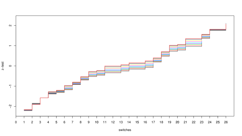
Figure 5: $z$-test values for different values of $\rho$

	$G_{0}$					$G_{1}$					$z$-test
1	1	$2^{+}$	3	4	$5^{+}$	6	7	$8^{+}$	9	$10^{+}$	-2.1901
2	1	$2^{+}$	3	4	6	$5^{+}$	7	$8^{+}$	9	$10^{+}$	-1.8797
3	1	$2^{+}$	3	6	4	$5^{+}$	7	$8^{+}$	9	$10^{+}$	-1.5791
4	1	$2^{+}$	6	3	4	$5^{+}$	7	$8^{+}$	9	$10^{+}$	-1.3374
5	1	6	$2^{+}$	3	4	$5^{+}$	7	$8^{+}$	9	$10^{+}$	-1.2602
6	6	1	$2^{+}$	3	4	$5^{+}$	7	$8^{+}$	9	$10^{+}$	-1.0872
7	6	1	$2^{+}$	3	4	7	$5^{+}$	$8^{+}$	9	$10^{+}$	-0.8729
8	6	1	$2^{+}$	3	7	4	$5^{+}$	$8^{+}$	9	$10^{+}$	-0.6236
9	6	1	$2^{+}$	7	3	4	$5^{+}$	$8^{+}$	9	$10^{+}$	-0.4107
10	6	1	7	$2^{+}$	3	4	$5^{+}$	$8^{+}$	9	$10^{+}$	-0.3533
11	6	7	1	$2^{+}$	3	4	$5^{+}$	$8^{+}$	9	$10^{+}$	-0.1873
12	6	7	1	$2^{+}$	3	4	$8^{+}$	$5^{+}$	9	$10^{+}$	-0.1873
13	6	7	1	$2^{+}$	3	$8^{+}$	4	$5^{+}$	9	$10^{+}$	-0.1096
14	6	7	1	$2^{+}$	$8^{+}$	3	4	$5^{+}$	9	$10^{+}$	-0.0175
15	6	7	1	$8^{+}$	$2^{+}$	3	4	$5^{+}$	9	$10^{+}$	-0.0175
16	6	7	$8^{+}$	1	$2^{+}$	3	4	$5^{+}$	9	$10^{+}$	0.0722
17	6	7	$8^{+}$	1	$2^{+}$	3	4	9	$5^{+}$	$10^{+}$	0.2798
18	6	7	$8^{+}$	1	$2^{+}$	3	9	4	$5^{+}$	$10^{+}$	0.5884
19	6	7	$8^{+}$	1	$2^{+}$	9	3	4	$5^{+}$	$10^{+}$	0.8718
20	6	7	$8^{+}$	1	9	$2^{+}$	3	4	$5^{+}$	$10^{+}$	0.9208
21	6	7	$8^{+}$	9	1	$2^{+}$	3	4	$5^{+}$	$10^{+}$	1.1602
22	6	7	$8^{+}$	9	1	$2^{+}$	3	4	$10^{+}$	$5^{+}$	1.1602
23	6	7	$8^{+}$	9	1	$2^{+}$	3	$10^{+}$	4	$5^{+}$	1.4627
24	6	7	$8^{+}$	9	1	$2^{+}$	$10^{+}$	3	4	$5^{+}$	1.7874
25	6	7	$8^{+}$	9	1	$10^{+}$	$2^{+}$	3	4	$5^{+}$	1.7874
26	6	7	$8^{+}$	9	$10^{+}$	1	$2^{+}$	3	4	$5^{+}$	2.0898

Table 1: $z$-test values and $\rho=0.5$

5 Concluding remarks

This paper studies the monotonicity of the $G^{\rho}$ class of weighted logrank tests introduced by Harrington and Fleming (1982). We proved a convenient monotonicity property for the two-sample class of logrank tests. This property holds trivially for the special case where there are no right censored observations (the Wilcoxon test), but, while intuitively quite clear, its proof required care due to the right censoring affecting the data. One can utilise this property to derive optimal bounds for the test statistic in case of imprecise data; such uses will be investigated for particular applications and reported elsewhere. It is also worth investigation the construction of statistical tests for equality of survival functions based on the number of switches, in a way that is similar to tests for perfect ranking in ranked set sampling presented by Li and Balakrishnan (2008). It is also of interest to study the generalization of the monotonicity property for such tests with more than two groups of data, this is left as a topic for future research.

Appendix

Lemma 5.1

Let $x$ and $y$ be any two real numbers in an interval $[a,b]$, where $a<b$. Then if $x-a<y-a$ and $b-y<b-x$ then $x<y$.

• Proof: The setting is illustrated in the figure below.

  As $y-a=(x-a)+(y-x)$ and $b-x=(b-y)+(y-x)$, then in order for both inequalities to hold, the second term in the right hand side must be positive, i.e. $y-x>0$ thus $x<y$. $\Box$

We use the lemma above to prove that $\frac{O-E_{A}}{\sqrt{V_{A}}}>\frac{O-E_{B}}{\sqrt{V_{B}}}$. First we define the 4 differences $D_{1}$, $D_{2}$, $D_{3}$ and $D_{4}$, which is illustrated in the figure below, as

$$D_{1} =\frac{O-E_{B}}{\sqrt{V_{B}}}-\frac{O-E_{B}}{\sqrt{V_{A}}}$$

$$D_{2} =\frac{O-E_{A}}{\sqrt{V_{B}}}-\frac{O-E_{B}}{\sqrt{V_{B}}}$$

$$D_{3} =\frac{O-E_{A}}{\sqrt{V_{A}}}-\frac{O-E_{B}}{\sqrt{V_{A}}}$$

$$D_{4} =\frac{O-E_{A}}{\sqrt{V_{B}}}-\frac{O-E_{A}}{\sqrt{V_{A}}}$$

In order for the inequality $\frac{O-E_{A}}{\sqrt{V_{A}}}>\frac{O-E_{B}}{\sqrt{V_{B}}}$ to hold, both inequalities $D_{3}>D_{1}$ and $D_{2}>D_{4}$ must be hold. We can express $D_{2}$ and $D_{3}$ as

$$D_{2} =D_{4}+\left[\frac{O-E_{A}}{\sqrt{V_{A}}}-\frac{O-E_{B}}{\sqrt{V_{B}}}\right]$$

$$D_{3} =D_{1}+\left[\frac{O-E_{A}}{\sqrt{V_{A}}}-\frac{O-E_{B}}{\sqrt{V_{B}}}\right]$$

so $\frac{O-E_{A}}{\sqrt{V_{A}}}-\frac{O-E_{B}}{\sqrt{V_{B}}}$ has to be positive, therefore $\frac{O-E_{A}}{\sqrt{V_{A}}}>\frac{O-E_{B}}{\sqrt{V_{B}}}$.

References

- Gehan (1965) Gehan, E. A., 1965. A generalized wilcoxon test for comparing arbitrarily singly-censored samples. Biometrika 52 (1/2), 203–223.
- Harrington and Fleming (1982) Harrington, D. P., Fleming, T. R., 1982. A class of rank test procedures for censored survival data. Biometrika 69 (3), 553–566.
- Kaplan and Meier (1958) Kaplan, E., Meier, P., 1958. Nonparametric estimation from incomplete observations. Journal of the American Statistical Association 53, 457–481.
- Latta (1977) Latta, R. B., 1977. Generalized wilcoxon statistics for the two-sample problem with censored data. Biometrika 64 (3), 633–635.
- Li and Balakrishnan (2008) Li, T., Balakrishnan, N., 2008. Some simple nonparametric methods to test for perfect ranking in ranked set sampling. Journal of Statistical Planning and Inference 138 (5), 1325 – 1338.
- Lou and Lan (1998) Lou, W. W., Lan, K. G., 1998. A note on the gehan-wilcoxon statistic. Communications in Statistics - Theory and Methods 27 (6), 1453–1459.
- Mantel (1966) Mantel, N., 1966. Evaluation of survival data and two new rank order statistics arising in its consideration. Cancer chemotherapy reports 50 (3), 163–170.
- Oller and Langohr (2017) Oller, R., Langohr, K., 2017. FHtest: An R package for the comparison of survival curves with censored data. Journal of Statistical Software 81 (15), 1–25.
- Peto and Peto (1972) Peto, R., Peto, J., 1972. Asymptotically efficient rank invariant test procedures. Journal of the Royal Statistical Society. Series A (General) 135 (2), 185–207.
- Prentice (1978) Prentice, R. L., 1978. Linear rank tests with right censored data. Biometrika 65 (1), 167–179.
- Therneau (2015) Therneau, T. M., 2015. A Package for Survival Analysis in S. Version 2.38.