Traces, symmetric functions, and a raising operator:
a generating function for Cauchy’s enumeration formula

Abstract

The polynomial relationship between elementary symmetric functions (Cauchy enumeration formula) is formulated via a “raising operator” and Fock space construction. A simple graphical proof of this relation is proposed. The new operator extends the Heisenberg algebra so that the number operator becomes a Lie product. This study is motivated by natural appearance of these polynomials in the theory of invariants for Lax equations and in classical and topological field theories.

Keywords: symmetric functions, Fock space, raising operator, matrix manifolds, Lax equations, Lie algebra, Cauchy enumeration formula

1 Motivations

An endomorphism of a linear space $L$ may be characterized by its invariants with respect to some symmetry group, most generally $GL(n)$, $n=\dim L$. The basic invariants are the determinant and the trace, which are special cases of the coefficients of the secular equations (here called prodeterminants), but also include power traces. These invariants appear naturally in many areas of physics: power traces in the theory of integrable systems on Lie algebras (Lax equation), generalized determinants in classical field theory, and symmetrized traces in topological field theory (Chern classes), to mention a few.

Tradition reserves different invariants for different theories, but, since they can be viewed as symmetric functions evaluated at eigenvalues of the given endomorphism, they are related. In particular, prodeterminants can be expressed as polynomials in power traces, with the Cauchy enumeration formula giving the coefficients.

In these notes, we introduce a “raising operator” which allows one to construct the Cauchy coefficients in these polynomial relation. We study some of its properties.

Although this work is motivated by the invariants of endomorphisms, the results are valid also for the theory of symmetric functions in general. Sections 2 and 3 are reviews of the basic facts on prodeterminants and symmetric functions. Sections 4, 5 and 6 deal with new results.

2 Determinants and traces of an endomorphism

Determinant and trace are examples of invariants with respect to the adjoin action of the general linear group $GL(n)$ acting on a linear space $L$, that is

$${\rm Tr\,}gAg^{-1}={\rm Tr\,}A\qquad\qquad\det gAg^{-1}=\det A$$

for any endomorphism $A\in{\rm End\,}L$ of a linear space $L$ and $g\in GL(n)$. These generalize into two families of invariants. The elements of one, called power-traces, are defined

$$I_{k}={\rm Tr}\;A^{k},\qquad k=1,2,\ldots$$ (2.1)

The other family generalizes determinant; its elements, denoted by $J_{i}$, are defined as coefficients of the characteristic polynomial for the endomorphism $A$, namely

$${\rm det}\;(A-\lambda)=\sum_{i=0}^{n}(-\lambda)^{n-i}\ J_{i}$$ (2.2)

where $n=\dim L$. We shall call $J_{k}$ a prodeterminant of order $k$. In particular

$$\begin{array}[]{rcl}J_{1}(A)&=&{\rm Tr\,}A\quad(=I_{1}(A))\\ J_{n}(A)&=&\det A\end{array}$$

Remark: Generalized determinant (prodeterminant) can also be defined also as

$$J_{k}=\frac{(-1)^{n-k}}{(n-k)!}\quad\frac{d^{n-k}}{d\lambda^{n-k}}\;{\rm det}\;(A-\lambda)\big{|}_{\lambda=0}$$

or, in a more explicit form, as

$$J_{k}=\sum\;A[a_{1},a_{2},\ldots,a_{k}]$$ (2.3)

where $A[\ldots]$ denotes determinant of the $k\times k$ minor (submatrix) determined by the set of columns and rows indexed by the same subset $[a_{1},\ldots,a_{k}]$ of the set $[1,\ldots,n]$. The summation in (2.3) extends over all ${n\choose k}$ possible selections of such subsets.

Example: Let $A$ be a $3\times 3$ matrix

$$A=\left[\begin{array}[]{ccc}a&b&c\cr d&e&f\cr g&h&i\end{array}\right]$$

Then one has the following prodeterminants

$$\begin{array}[]{rcl}J_{1}&=&a+e+i\\[2.0pt] J_{2}&=&\det\left[\begin{smallmatrix}a&b\cr d&e\end{smallmatrix}\right]+\det\left[\begin{smallmatrix}a&c\cr g&i\end{smallmatrix}\right]+\det\left[\begin{smallmatrix}e&f\cr h&i\end{smallmatrix}\right]\\[2.0pt] J_{3}&=&\det A\end{array}$$

while the power-traces are

$$\begin{array}[]{rcl}I_{1}&=&a+e+i\\ I_{2}&=&a^{2}+e^{2}+i^{2}+2db+2gc+2fh\\ I_{3}&=&a^{3}+e^{3}+i^{3}+3abd+3cdg+3bde\\ &&+3efg+3bfh+3fgi+3ach+3chi\end{array}$$

Particular applications in systems with symmetries favor one of the two types of invariants, like Lax equations use rather $I$ while the theory of Chern classes and some particle models — $J$ (see Appendix A). But, in fact, the two are dependent:

$$\begin{array}[]{rcl}J_{1}&=&I_{1}\cr 2J_{2}&=&I_{1}^{2}-I_{2}\cr 6J_{3}&=&I_{1}^{3}-3I_{1}I_{2}+2I_{3}\cr 12J_{4}&=&I_{1}^{4}-6I_{1}^{2}I_{2}+8I_{1}I_{3}+3I_{2}^{2}-6I_{4}\cr\ldots&\end{array}$$ (2.4)

The polynomials on the right side of (2.4) will be denoted by $j$ and called Cauchy polynomials — they are the central topic of this note. The question is to determine the coefficients of these polynomials. They are known to be directly related to the rank of the conjugacy classes of the symmetric group (group of permutations). Section 4 will present a new formula generating the polynomials with the corresponding coefficients. But first, we review some basic facts about symmetric functions.

3 Symmetric functions and Cauchy formula

Connection of the invariants with the symmetric functions follows directly from the fact that if an endomorphism $A$ has a diagonal matrix form in some basis, with eigenvalues on the diagonal

$$A=\left[\begin{matrix}\lambda_{1}&0&\ldots&0\cr 0&\lambda_{2}&\ldots&0\cr\vdots&\vdots&\ddots&\cr 0&0&&\lambda_{n}\end{matrix}\right]\,,$$

then clearly

$$I_{k}=\sum_{i}^{n}\;\lambda_{i}^{k}$$

and

$$J_{k}=\sum\;\lambda_{a_{1}}\cdot\lambda_{a_{2}}\cdot\ldots\cdot\lambda_{a_{k}}\,,$$

where the last sum runs over all $n\choose k$ selections of $k$ among the set of the $n$ eigenvalues $\lambda$ of the endomorphism $A$. These expressions can easily be recognized as the symmetric functions evaluated on the set of eigenvalues of $A$. Invariants $I$ and $J$ corresponds to the two types of basic symmetric functions. Consequently, relations (2.4) may be understood as a transformation formula for the change of basis of the space of symmetric functions.

Let us recall some basic facts about symmetric functions. The space of symmetric functions of degree $k$ is denoted by ${\mathcal{S}}_{k}$. The three most frequently used families of basic symmetric functions in variables $x_{1},x_{2},\ldots,x_{n}$ are these:

A. Elementary symmetric functions:

$$c_{k}=\sum\;x_{i_{1}}x_{i_{2}}\ldots x_{i_{k}}\qquad\qquad 1\leq i_{1}<i_{2}<\ldots<i_{k}\leq n$$

B. Power sums:

$$s_{k}=x_{1}^{k}+x_{2}^{k}+\ldots+x_{n}^{k}\qquad\qquad\phantom{1\leq i_{1}<i_{2}<\ldots<i_{k}\leq n}$$ (3.1)

C. Wronski functions:

$$w_{k}=\sum\;x_{i_{1}}x_{i_{2}}\ldots x_{i_{k}}\qquad\qquad 1\leq i_{1}\leq i_{2}\leq\ldots\leq i_{k}\leq n$$

The number $n$ of variables in these definitions may essentially be unrestricted — one can always set $x_{i}=0$ for $i>n$. Here is an example of the basic symmetric functions of degree 1, 2 and 3 in three variables:

$$\begin{array}[]{rcl}c_{1}=s_{1}=w_{1}&=&x_{1}+x_{2}+x_{3}\\[6.0pt] c_{2}&=&x_{1}x_{2}+x_{2}x_{3}+x_{1}x_{3}\\ s_{2}&=&x_{1}^{2}+x_{2}^{2}+x_{3}^{2}\\ w_{2}&=&x_{1}^{2}+x_{2}^{2}+x_{3}^{2}+x_{1}x_{2}+x_{2}x_{3}+x_{1}x_{3}\\[6.0pt] c_{3}&=&x_{1}x_{2}x_{3}\\ s_{3}&=&x_{1}^{3}+x_{2}^{3}+x_{3}^{3}\\ w_{3}&=&x_{1}^{3}+x_{2}^{3}+x_{3}^{3}+x_{1}x_{2}x_{3}+x_{1}^{2}x_{2}+x_{1}x_{2}^{2}\\ &&+x_{1}^{2}x_{3}+x_{1}x_{3}^{2}+x_{2}^{2}x_{3}+x_{2}x_{3}^{2}\end{array}$$

Definition 3.1

By $\lambda\vdash k$ we denote a fact that the set $\lambda=(\lambda_{1},\lambda_{2},\ldots)$ is a partition of natural number $k$, that is:

$$\begin{array}[]{rl}&\lambda_{1}+\lambda_{2}+\ldots+\lambda_{k}=k\cr&\lambda_{1}\leq\lambda_{2}\leq\ldots\leq\lambda_{k}\end{array}$$

A partition can alternatively be described by a partition symbol $\alpha=[\alpha_{1},\alpha_{2},\ldots,\alpha_{k}]$ in which $\alpha_{i}$ denotes the number of i’s among the elements of set $\lambda$. Thus

$$1\cdot\alpha_{1}+2\cdot\alpha_{2}+\ldots+k\cdot\alpha_{k}=k$$

By $\alpha\models k$ we denote that $\alpha$ is a partition symbol of $k$.

Example: Number $10$ admits partition $1+1+1+3+4=10$, thus we write $(1,1,1,3,4)\vdash 10$. For the partition symbol we write $[3,0,1,1]\models 10$.

The fundamental theorem of symmetric functions states that basis of the space of homogeneous symmetric functions of degree $k$ may be composed from products of members of any of these families. If $b_{i}$ denotes the members of any of the families of the basic functions (3.1), then the set of products

$$\{\;b_{1}^{\alpha_{1}}\cdot b_{2}^{\alpha_{2}}\cdot\cdots\cdot b_{k}^{\alpha_{k}}\mid\alpha{\scriptstyle\models}k\;\}$$

forms a basis of the space ${\mathcal{S}}_{k}$ of symmetric functions of degree $k$. The relation between the types of symmetric functions is well known (see, e.g., [9]). In particular:

Theorem 3.2

Any elementary symmetric function can be expressed as a linear combination of products of the power sums:

$$c_{k}=\sum_{\alpha\models k}\;(-1)^{\alpha_{2}+\alpha_{4}+\ldots}\;\cdot\frac{h(\alpha)}{n!}\;\cdot s_{1}^{\alpha_{1}}\cdot s_{2}^{\alpha_{2}}\cdot\ldots\cdot s_{k}^{\alpha_{k}}$$

where the sum runs over all partitions of $k$ and where $h(\alpha)$ is known as Cauchy formula, is given by

$$h(\alpha)=\frac{n!}{\alpha_{1}!\alpha_{2}!\cdot\cdot\cdot\alpha_{k}!\;\cdot\;1^{\alpha_{1}}2^{\alpha_{2}}\cdots k^{\alpha_{k}}}\ .$$

This theorem provides the coefficients of the polynomial expansion of prodeterminants in terms of traces, (Eq. 2.4).

Interestingly, the relation between Wronski functions $w$ and power sums $s$ utilizes the same Cauchy formula, but without alternating sign:

$$w_{k}=\sum_{\alpha\models k}\;\frac{h(\alpha)}{n!}\;s_{1}^{\alpha_{1}}\cdot s_{2}^{\alpha_{2}}\cdot\ldots\cdot s_{k}^{\alpha_{k}}$$

Proofs of this statements involve usually a rather unpleasant juggling with sums, indices, and logarithms [9]. In the next section, we shall give a different derivation on Cauchy coefficients. An alternative simple proof will be provided in Section 6.

Remark 3.3

Cauchy formula appears naturally in yet another context, namely in the theory of symmetric groups. It is well known that any element of symmetric group $S_{n}$ can be written as a product of cyclic permutations. Two elements of $S_{n}$ belong to the same adjoint class if both are composed from cycles of the same length. From this, it immediately follows that a conjugacy class may be labeled uniquely by a partition of $n$, say by a partition symbol $\alpha=[\alpha_{1},\alpha_{2},\ldots,\alpha_{n}]$, and that the size of the corresponding class is

$$h(\alpha)=\frac{n!}{\alpha_{1}!\,\alpha_{2}!\cdots\alpha_{k}!\,\cdot\,1^{\alpha_{1}}2^{\alpha_{2}}\cdots k^{\alpha_{k}}}$$

This is a straightforward enumeration formula. Typically, these two appearances of Cauchy formula — in the theory of symmetric functions and in symmetric group — are left unrelated. Our proof of the prodeterminant-trace formula is actually based on the combinatorial meaning of the Cauchy formula.

4 Fock construction for Cauchy polynomials (main result)

In this section we provide some insight into the structure of relations (2.4) in terms a Fock space construction. Here we abstract from the functional meaning of the components of these relations, but rather we will treat these relations as polynomials on their own. In particular, polynomials (2.4) are obtained in a recursive process of raising a “vacuum” state in the space of multivariate polynomials. (Not to be confused with the raising operator appearing in a related context, like in [2]).

Let ${\mathcal{P}}[x]$ be a linear space of finite polynomials over variables $x_{1}$, $x_{2}$, $x_{3}\ldots$ etc. We shall use the multi-index notation $(n)=(n_{1},n_{2},\ldots)$. The monomials

$$x^{(n)}=x_{1}^{n_{1}}\;x_{2}^{n_{2}}\;x_{3}^{n_{3}}\ldots$$

form a basis of ${\mathcal{P}}[x]$, and a general element of ${\mathcal{P}}[x]$ is

$$p(x)=\sum_{(n)}\;c_{(n)}\;x^{(n)}$$

with some coefficients $c_{(n)}$. We shall also use Dirac notation and write $x^{(n)}=|n_{1},n_{2},\ldots\rangle$, so that

$$p(x)=\sum_{(n)}c_{(n)}|n\rangle$$

Clearly, $c_{(n)}=\langle\;n\;|\;p(x)\;\rangle$.

Definition 4.1

Derivation operator $\delta\in{\rm End\,}{\mathcal{P}}[x]$ is defined by its action on a single variable and by Leibniz rule

$$\begin{array}[]{rl}(i)&\delta\;x_{k}=k\,x_{k+1}\\ (ii)&\delta\;(ab)=\delta a\cdot b+a\cdot\delta b\end{array}$$ (4.1)

Proposition 4.2

For a simple power $x_{k}^{n}$ and for a general monomial, one has respectively the following formulae

$$\begin{array}[]{rl}(i)&\delta\;x_{k}^{n}=nk\,x_{k}^{n-1}\,x_{k+1}\\[4.0pt] (ii)&\delta\;x^{(n)}=\displaystyle\sum_{{i:\ n_{i}>0}}i\cdot n_{i}\cdot x^{(n)}\cdot x_{n_{i+1}+1}\;/\;x_{n_{i}}\,.\end{array}$$ (4.2)

The last formula can be written in Dirac notation as

$$\delta\;|n_{1},n_{2},\ldots\rangle=\sum_{i}\;i\,n_{i}\;|n_{1},n_{2},\ldots,n_{i-1},n_{i}-1,n_{i+1}+1,n_{i+2},\ldots\;\rangle$$ (4.3)

where the sum extends over the terms for which $n_{i}>0$. (Or, equivalently, one can simply set $|n_{1},n_{2},\ldots\rangle=0$ whenever $n_{i}<0$ for some $i$).

We shall now define a raising operator $\Delta^{-}\in{\rm End\,}\mathcal{P}[x]$ by

$$\Delta^{-}=\hat{x}_{1}-\delta\ ,$$ (4.4)

where $\hat{x}_{1}$ denotes operator of multiplication by variable $x_{1}$. Consider a sequence of polynomials (coherent states) determined by a consecutive application of the raising operator $\Delta^{-}$, namely

$$\begin{array}[]{rl}(i)&\quad j_{1}\;(x)=x_{1}\cr(ii)&\quad j_{k+1}(x)=\Delta^{-}j_{k}=(\hat{x}_{1}-\delta)j_{k}\ .\end{array}$$ (4.5)

One can easily generate the following sequence of polynomials:

$$\begin{array}[]{rcl}j_{1}(x)&=&x_{1}\cr j_{2}(x)&=&x_{1}^{2}-x_{2}\cr j_{3}(x)&=&x_{1}^{3}-3x_{1}x_{2}+2x_{3}\cr j_{4}(x)&=&x_{1}^{4}-6x_{1}^{2}x_{2}+8x_{1}x_{3}+3x_{2}^{2}-6x_{4}\cr j_{5}(x)&=&x_{1}^{5}-10x_{1}^{3}x_{2}+20x_{1}^{2}x_{3}+15x_{1}x_{2}^{2}-30x_{1}x_{4}-20x_{2}x_{3}+24x_{5}\cr\ldots&\end{array}$$ (4.6)

where the first polynomial $j_{1}=x_{1}$ may be viewed as a “vacuum state” and $j_{k}=\Delta^{k}j_{1}$ as the $k$-th “excited state” obtained via the raising operator $\Delta^{-}$. One may easily recognize in the above the polynomials (2.4):

Theorem 4.3

The system determined by raising operator $\Delta^{-}$ and Fock space construction (4.5) coincides with Cauchy polynomials. In particular, let $A\in{\rm End\,}L$ be an endomorphism of a linear space. Denote $I_{i}={\rm Tr\,}A^{i}$. Then the $k$-th prodeterminant $J_{k}(A)$ is

$$J_{k}(A)=\frac{1}{k!}\;j_{k}(I_{1},I_{2},...,I_{k})$$

A graphical proof of this theorem is provided in section 6.

Remark 4.4

The family of polynomials $j_{i}$ together with the raising operator $\Delta^{-}$ may be interpreted and studied as a so-called Appell system (see [5]).

One may define a complementary raising operator

$$\Delta^{+}=\hat{x}_{1}+\delta$$

and the corresponding sequence of polynomials

$$\begin{array}[]{rl}(i)&\quad k_{1}(x)=x_{1}\cr(ii)&\quad k_{i+1}(x)=(\hat{x}_{1}+\delta)k_{i}\end{array}$$

Interestingly enough, the absolute values of the coefficients of these two types of polynomials coincide, i.e.

$$\langle\;j(x)\mid{\bf n}\;\rangle=\pm\;\langle\;k(x)\mid{\bf n}\;\rangle$$

Thus $\Delta^{+}$ enumerates directly the conjugacy classes of symmetric group:

Corollary 1

The number of elements of the conjugacy class of symmetric group $S_{n}$ corresponding to a partition symbol $\alpha\models n$ (i.e., consisting of elements that are composition of cycles in which cycle of length $i$ appears $\alpha_{i}$ times) is a coefficient at $x^{(\alpha)}$ of the generating function

$$(x_{1}+\delta)^{(\alpha_{1}+\ldots+\alpha_{k})}\;x_{1}=\sum\;c_{(\alpha)}\;x^{(\alpha)}$$

or, in Dirac notation,

$$\langle\;(x_{i}+\delta)^{(\alpha_{1}+\ldots+\alpha_{k})}x_{1}\mid\alpha_{1},\ldots,\alpha_{k}\;\rangle=\sum_{|\alpha\rangle}\;c_{n}\;|\alpha_{1},\ldots,\alpha_{k}\;\rangle$$

5 Lie algebra

The operators $\hat{x}_{i}$ of multiplication by $x_{i}$, the partial derivatives $\partial_{i}\equiv\partial/\partial x_{i}$ with respect to $x_{i}$ and identity, all acting in the space of polynomials ${\mathcal{P}}[x]$, form Heisenberg Lie algebra ${\mathcal{H}}$, the algebra of the harmonic oscillator. By including the derivation $\delta$ defined in (4.1), this algebra may be extended to a Lie algebra

$$\bar{\mathcal{H}}=\hbox{gen}\,\{\partial_{i},\,\hat{x}_{j},\,\delta\}\,.$$ (5.1)

with the following commutation relations for the generators:

$$\begin{array}[]{rcl}[\;\partial_{i},\;\hat{x}_{j}\;]&=&\delta_{ij}\cr[\;\delta,\;\hat{x}_{j}\;]&=&j\cdot\hat{x}_{j+1}\cr[\;\partial_{j},\;\delta\;]&=&j\cdot\hat{x}_{j+1}\cdot\hat{x}_{j}^{-2}\end{array}$$

It is easy to calculate the Lie bracket of the two raising operators:

$$[\;\Delta^{-},\;\Delta^{+}\;]=2x_{2}\delta$$

Consider a subspace ${\mathcal{J}}[x]\subset{\mathcal{P}}[x]$ spanned by polynomials $\{j_{1},j_{2},\ldots\}$ of Equation (4.6). By definition, $\Delta^{-}$ is a raising operator in the subspace ${\mathcal{J}}[x]$. The derivative with respect to the first variable acts as a lowering operator:

$$\partial_{1}j_{n}=n\cdot j_{n-1}$$

Derivative with respect to the $k$-th variable lowers the index by $k$:

$$\partial_{k}j_{n}={n\choose k}\cdot j_{n-k}$$

Recall that the number operator is an operator $N$ in the Fock space, defined on basis elements by $Nj_{k}=k\cdot j_{k}$ (eigenvectors). In the context of the standard Heisenberg algebra, the number operator does not lie in the Lie algebra, and must be defined as an element of the enveloping algebra, namely as a product $N=\hat{x}\partial$. It is remarkable that the Lie algebra $\hat{\mathcal{H}}$ (5.1) does contain the number operator, since

$$[\;\partial_{1},\;\Delta^{-}\;]j_{n}=n\;j_{n}$$

In general, one has:

$$\begin{array}[]{rcl}[\;\Delta^{-},\;\partial_{k}\;]\;j_{n}&=&(-)^{k}\;{n\choose k}\;j_{n}\\[4.0pt] [\;\Delta^{+},\;\partial_{k}\;]\;k_{n}&=&{n\choose k}\;k_{k}\end{array}$$

6 Graphic representation

Prodeterminants (2.2) can equivalently be defined as “averages” over traces:

$$J_{k}=\frac{1}{k!}\sum_{\sigma\in S_{k}}\;\hbox{sgn\,}(\sigma)\;A^{i_{1}}_{\sigma(i_{1})}\;A^{i_{2}}_{\sigma(i_{2})}\,\cdots\,A^{i_{k}}_{\sigma(i_{k})}$$

where an additional sum over repeated indices of terms is understood (Einstein’s summation convention) (cf. Appendix A). This leads to a more geometric formulation of the algebraic objects discussed. Here we show how a simple proof of Theorem 3.2 on the Fock space structure of Cauchy polynomials (Appell system) may be obtained using a graphical language for the category of tensor spaces. It also ties symmetric functions with the combinatorial meaning of the Cauchy formula of Remark 3.3.

In spirit, the graphical language for tensor contractions that we want to use is cognate with a number of approaches related to the language of tensor operads like that of [11], [4], [10], or [6]. Such a graphical language — besides the conceptual value — may lead to nice simplifications of proofs, like the one we present.

Here, we represent an endomorphism $A$ by a square with two arrows, one going out and one going in. The arrows may be viewed as representing indices, upper and lower, respectively, if $A$ is represented by a matrix. In general, the arrows represent “slots” of $A$ viewed as a tensor, contravariant and covariant, respectively. A vector will be represented by a square with a single arrow out (“contravariant slot”); and a linear form (covector), by a single arrow in (“covariant slot”). Figure 1 shows graphical representation of basic linear operations (contractions).

Figure 1: Contractions of tensors

The trace and power-traces can be viewed as seen in Figure 2.

Figure 2: Power traces of an endomorphism $A$

The prodeterminants $J_{k}$ are obtained as follows. Consider a tensor product of $k$ copies of $A$, namely the $(k,k)$-type tensor $A\otimes A\ldots\otimes A$ (left side of Figure 3). One can take a trace of this operator by closing the $k$ out-arrows with the $k$ in-arrows . There are $k!$ such possible pairings of the $k$ arrows with the $k$ slots.

Figure 3: Tensor product $A^{\otimes n}$ and alternating tensor $\wedge$

Scalar $J_{k}$ is obtained by taking a sum over all possibilities (permutations), each term assuming the sign corresponding to the parity of the permutation. In other words, we contract $A\otimes A\otimes\ldots\otimes A$ with the $(k,k)$-type alternating tensor “$\wedge$”, totally antisymmetric in both sectors (represented in the right side of Figure 3). Figure 4 illustrates the case of $J_{2}$.

Figure 4: The origin for the second Cauchy polynomial.

This gives the formula relating generalized determinants with power-traces! In a similar simple combinatorial play with strings one obtains the next invariant $J_{3}$, see Figure 5.

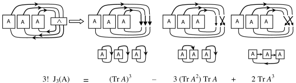
Figure 5: The origin of the third Cauchy polynomial.

The general form of Cauchy polynomials as a result of the action of the raising operator (4.4) emerges by induction and combinatorial meaning of the above tensor contractions. Indeed, increasing the number of the “tensor boxes” on the left side on any of the last three figures will add under contraction two types of new graphical loops: either the new tensor makes a single loop with itself, or it will get in the path of one of the existing loops increasing their length by one. The former case corresponds to the operator $\hat{x}_{1}$ in (4.4), the latter to $\delta$.

Appendix

A. Geometric definition of prodeterminant

Given linear space $L$ of dimension $d$. Consider Grassmann space (tensor space)

$$\wedge^{k}L=L\wedge L\wedge\ldots\wedge L$$

Any endomorphism $A\in{\rm End\,}L$ has a natural extension to an endomorphism $A^{\wedge k}\in{\rm End\,}\wedge^{k}L$ which for a simple multi-vector $v_{1}\wedge v_{2}\wedge\dots\wedge v_{k}$ is defined

$$A^{*}(v_{1}\wedge v_{2}\wedge\dots\wedge v_{k})=A(v_{1})\wedge A(v_{2})\wedge\dots\wedge A(v_{k})$$

Note that if $\{e_{i}\}$ is a basis of $L$, and $\{\epsilon_{i}\}$ is the dual basis of $L^{*}$, then $A=\epsilon^{i}A_{i}^{j}e_{j}$, and

$$A^{\wedge k}=A\wedge A\wedge\dots\wedge A=A_{i_{1}}^{j_{1}}A_{i_{2}}^{j_{2}}\ldots A_{i_{k}}^{j_{k}}\;e_{j_{1}}\wedge e_{j_{2}}\wedge\ldots\wedge e_{j_{k}}\otimes\epsilon^{i_{1}}\wedge\epsilon^{i_{2}}\wedge\ldots\wedge\epsilon^{i_{k}}$$

Since multi-vectors $e_{j_{1}}\wedge e_{j_{2}}\wedge\ldots\wedge e_{j_{k}}$ form a basis in the Grassmann space, the formula for prodeterminant can be easily written as a trace of the induced endomorphism

$$J_{k}(A)={\rm Tr\,}A^{\wedge k}$$

In particular, $J_{1}(A)={\rm Tr\,}A$ and $J_{n}(A)={\rm Tr\,}A^{\wedge n}$.

B. Matrix manifolds

Consider orbits of the adjoint action of the general linear group $GL(n)$ acting on the space of endomorphisms ${\rm End\,}(L)$ over some field of some space $L$ of dimension $\dim L=n$:

$$g:\;M\longrightarrow gMg^{-1}$$

The $n\times n$ dimensional space ${\rm End\,}\cong\mathbb{R}^{n\times n}$ is foliated by the orbits of this action, which we call matrix manifolds (see [8], where the case of complex spaces is considered). Thus the prodeterminants $J_{k}$ are invariant with respect to this action and they are natural objects to consider in this context. In particular, a set of $n$ values determines an orbit (that is, the set of orbits is parameterized by the values of $J$’s). If a matrix $M$ is an element of some orbit $\mathcal{O}_{M}$, then

$${\rm Ker\,}J_{1}(M)\cap{\rm Ker\,}J_{2}(M)\cap\ldots\cap{\rm Ker\,}J_{n}(M)=T_{M}{\mathcal{O}}$$ (6.1)

For more (the role played by the rank of $M$ and for applications in field theory), see [8].

Lax equation

Consider a matrix representation of Lie algebra $L$ and a dynamical system

$$\dot{M}=[M,B]$$

The power-traces of $M$ provide natural invariants (called Casimir invariants) of the Lax dynamical system. Indeed

$$\begin{array}[]{rcl}\frac{d}{dt}\;{\rm Tr\,}M^{n}&=&n\;{\rm Tr\,}\dot{M}M^{n-1}=n{\rm Tr\,}[M,B]M^{n-1}\cr&=&n({\rm Tr\,}MBM^{n-1}-{\rm Tr\,}BMM^{n-1})=0\end{array}$$

In particular, one can consider the adjoint representation of $L$ and then $M$ and $B$ are directly elements of $L$. Let $L$ be a Lie algebra. In [7] we consider the space of $L$ as a manifold and define a (1,1)-type tensor field (a field of endomorphisms) by

$$A_{x}(\tilde{v})=({\rm ad\,}_{x}v)^{\sim}=[x,v]^{\sim}$$

If $x^{i}$ are (linear) coordinates on $L$ then

$$A=x^{i}\;c_{ij}^{k}\;\frac{\partial}{\partial x^{k}}\otimes dx^{j}$$

At every point $a\in L$, tensor $A$ can be viewed as an endomorphism of the tangent space, $A:T_{a}L\to T_{a}L$. One can define a distribution $\Im A\subset TL$. It is easy to show that this distribution is integrable; the integral manifolds ${\mathcal{O}}$ coincide with the orbits of the adjoint action of $L$, and:

$$\Im A=T{\mathcal{O}}$$

The power-traces of the adjoint representation provide a set of scalar functions $I_{i}:\;L\to\mathbb{R}$. One of them, $I_{2}$, is the Killing form (known in this context as Cartan quadratic function)

$$I_{2}(a)=K(a,a)=c_{ip}^{q}c_{qj}^{p}a^{i}a^{j}$$

Constant value of the Killing function determine a pseudosphere (hyperbolic sphere — in the case of semi-simple algebras). Orbits of the adjoint action of the corresponding Lie group lie in these spheres. They lie inside the surfaces determined by all the higher-order power-traces. Thus, if for a set of $n$ numbers $r$ we define a submanifold of $L$

$$S(r_{1},\ldots,r_{n})=\{\;a\in L\mid I_{1}(a)=r_{1},\ldots,I_{n}(a)=r_{n}\;\}$$

then at any point $a\in L$

$${\mathcal{O}}_{a}\subset S(I_{1}(a),\ldots,I_{n}(a))$$

Given vector field $B$ on $L$, define a new vector field of a dynamical system

$$X_{B}=A\,\vrule height=6.0pt,width=0.4pt,depth=0.0pt\vrule width=6.0pt,height=0.1pt,depth=0.0pt\,B$$

Thus we have a corollary: every Lax dynamical system on $L$ preserves each $I_{i}$ as the first integral of motion. Indeed:

$$X_{B}f=df\,\vrule height=6.0pt,width=0.4pt,depth=0.0pt\vrule width=6.0pt,height=0.1pt,depth=0.0pt\,X_{B}=df\,\vrule height=6.0pt,width=0.4pt,depth=0.0pt\vrule width=6.0pt,height=0.1pt,depth=0.0pt\,A\,\vrule height=6.0pt,width=0.4pt,depth=0.0pt\vrule width=6.0pt,height=0.1pt,depth=0.0pt\,B=0$$

References

- [1] Arnol’d, V.I., The Hamiltonian nature of the Euler equations in the dynamics of a rigid body and an ideal fluid, Usp. Mat. Nauk, 24, pp. 225-226 (1969), (in Russian).
- [2] F. Bergeron and A. Garsia, Science Fiction and Macdonald Polynomials, in Algebraic methods and q-special functions (eds. R. Floreanini, L. Vinet, CRM Proceedings & Lecture Notes, Am. Math. Soc., 22, pp. 1-52 (1999).
- [3] David H. Collingwood & William M. McGovern, Nilpotent Orbits in Semisimple Lie Algebras, (Van Nostrand Reinhold, New York, 1992).
- [4] Predrag Cvitanović, Group theory for Feynman diagrams in non-Abelian gauge theories, Phys. Rev. D, 14 (6) pp. 1536–1553 (1976).
- [5] Philip Feinsilver, Jerzy Kocik and Rene Schott, Representations of the Schroedinger algebra and Appell systems, Fortschritte der Physik, 52 (4) pp. 343-359 (2004).
- [6] Louis H. Kauffman, Knots and Physics, (World Scientific Pub., 1991).
- [7] Jerzy Kocik, Natural endomorphism field on a Lie algebra, Journal of Generalized Lie Theory and Applications, Vol. 4 (2010), Art. ID G100302,
- [8] Jerzy Kocik & Jan Rzewuski: Structure of Matrix Manifolds and a Particle Model, Journal of Mathematical Physics, 37 (2), pp. 1004-1028 (1996).
- [9] Walter Lederman, Introduction to group characters (second edition), (Cambridge University Press, Cambridge, 1987).
- [10] Zbigniew Oziewicz, Operad of graphs, convolution and quasi Hopf algebra, Contemporary Mathematics, 318, pp. 175–197 (2003) .
- [11] Roger Penrose, Applications of Negative Dimensional Tensors. In Combinatorial Mathematics and its Applications (ed. DJA Welsh, Academic Press, 1971), pp. 221-224.