Fast computation of all pairs of geodesic distances

Abstract

Computing an array of all pairs of geodesic distances between the pixels of an image is time consuming. In the sequel, we introduce new methods exploiting the redundancy of geodesic propagations and compare them to an existing one. We show that our method in which the source point of geodesic propagations is chosen according to its minimum number of distances to the other points, improves the previous method up to 32 % and the naive method up to 50 % in terms of reduction of the number of operations.

1 Introduction

An array of all pairs of geodesic distances, between nodes of a graph, is very useful for several applications such as clustering by kernel methods or graph-based segmentation or data analysis. However, computing this array of distances is time consuming. That is the reason why two new methods, that fill in a fast way the distances array, are presented and compared in this paper.

Our methods are available on general graphs. In this paper we present them on images of which the pixels are considered as the nodes of the graph and the links between the neighbors corresponds to the edges of the graph.

In image processing, it is interesting to use the geodesic distance between pixels in place of another distance. The array of all pairs of geodesics distances allows to segment an image in geodesically connected regions (i.e., geodesic balls) (Noyel et al., 2007b). All pairs of geodesic distances are also useful on defining adaptive neighborhoods of filters used for edge-preserving smoothing (Lerallut et al., 2007; Bertelli and Manjunath, 2007; Grazzini and Soille, 2009). Nonlinear dimensionality reduction techniques are mostly based on multidimensional scaling on a Gram matrix of distances between the pairs of variables. Particularly interesting for estimating the intrinsic geometry of a data manifold is the Isometric feature mapping Isomap (Tenenbaum, 1998; Tenenbaum et al., 2000). After defining a neighborhood graph of variables, Isomap calculates the shortest path between every pairs of vertices, which is then low-dimensional embedded via multidimensional scaling. The application of Isomap to hyperspectral image analysis requires the computation of all pairs of geodesic distances for a graph of all the pixels of an image (Mohan et al., 2007).

However, the computation of all pairs of geodesic distance in an image is time consuming. In fact, the naive approach consists in repeating $N$ times the algorithm to compute the geodesic distance from each of the $N$ pixels to all others. Computing the geodesic distance from one pixel to all others is called a geodesic propagation. The pixel at the origin of a propagation is called the source point and the array containing all pairs of geodesic distances is named the distances array. Therefore, the naive approach is of complexity $O(N\times M)$, with $M$ the complexity of a geodesic propagation. Several algorithms for geodesic propagations are available: the most famous is the Fast Marching Algorithm introduced by Sethian (1996, 1999) and of complexity $O(N\log(N))$. This algorithm consists in computing geodesic distances in a continuous domain, using a first order approximation, to obtain the distance in the discrete domain. Another algorithm was developed by Soille (1991) for binary images and for grey level images (Soille, 1992). In order to compare our results, we will use the Soille’s algorithm of “geodesic time function” (Soille, 1994, 2013). Recent implementations of Soille’s algorithm for binary images are in $O(N\log(N))$ (Coeurjolly et al., 2004). Bertelli et al. (2006) have introduced a method to exploit the redundancy when several geodesic propagations are computed. In fact, when we perform a geodesic propagation from one pixel, all the geodesic paths from this pixel are stored in a tree. Using this tree, we know all the geodesic distances between any pairs of points along the geodesic path connecting two points. This redundancy is also exploited in earlier algorithm for computing the propagation function well known in mathematical morphology (Lantuejoul and Maisonneuve, 1984).

In order to choose the source points of the geodesic propagations, Bertelli et al. (2006) have proposed to select them randomly in a spiral like order starting from the edges of the image and going to the center. In the sequel, we test several deterministic approaches to select the source points and we show that a method based on the filling rate of the distances array can reduce the number of operations up to 32 % compared to Bertelli et al. (2006) method.

After discussing some prerequisites about the definition of a graph on an image, the geodesic distances and the exploitation of redundancy between geodesic propagations, we introduce several methods of computation of all pairs of distances and we compare them.

2 Prerequisites

An image $f$ is a discrete function defined on the finite domain $E\subset\mathbb{N}^{2}$, with $\mathbb{N}$ the set of positive integers. The values of a gray level image belongs to $\mathcal{T}\subset\mathbb{R}$. For a color image (i.e. with 3 channels) the values are in $\mathcal{T}^{3}=\mathcal{T}\times\mathcal{T}\times\mathcal{T}$ and for a multivariate image of $L$ channels the values are in $\mathcal{T}^{L}$. In what follows, we consider $\mathcal{T}\subset\mathbb{R}^{+}$. The whole results presented in the current paper are directly extendable to color or multivariate images (Noyel et. al. 2007a, 2007b), (Noyel, 2008).

An image is represented on a grid on which the neighborhood relations can be defined. Therefore, an image is seen as a non oriented graph $G=\{V_{G},E_{G}\}$ in which the vertices $V_{G}$ correspond to the coordinates of pixels, $V_{G}\in\mathbb{Z}\times\mathbb{Z}$, and the edges, $E_{G}\in\mathbb{Z}^{2}$, give the neighborhood relations between the pixels. Then, the notion of neighborhood of a pixel $p$ in the grid is introduced as the set of pixels which are directly connected to it:

$$\forall p,q\in V_{G},\hskip 14.22636ptp\text{ and }q\text{ are neighbors }\Leftrightarrow(p,q)\in E_{G},$$ (1)

where the ordered pair $(p,q)$ is the edge which joins the points $p$ and $q$. We assume that a pixel is not its own neighbor and the neighboring relations are symmetrical. The neighborhood of pixel $p$, $N_{G}(p)$, defined a subset of $V_{G}$ of any size, such as:

$$\forall p,q\in V_{G},\hskip 14.22636ptN_{G}(p)=\{q\in V_{G},\hskip 2.84526pt(p,q)\in E_{G}\}.$$ (2)

Usually in image processing, the following neighborhoods are defined: 4-neighborhood, 8-neighborhood or 6-neighborhood. In the sequel, we use the 8-neighborhood. For our study, the choice of the neighborhood has no influence since we compare several methods using for each one the same neighborhood.

A path between two points $x$ and $y$ is a chain of points $\left(x_{0},x_{1},\ldots,x_{i},\ldots,x_{l}\right)\in E$ such as $x_{0}=x$ and $x_{l}=y$, and for all $i$, $(x_{i},x_{i+1})$ are neighbours. Therefore, a path $(x_{0},x_{1},\ldots,x_{l})$ can be seen as a subgraph in which the nodes corresponds to the points and the edges are the connections between neighbouring points.

The geodesic distance $d_{geo}(x_{0},x_{l})$, or geodesic time, between two points of a graph, $x_{0}$ and $x_{l}$, is defined as the minimum distance, or time, between these two points, $\inf_{\mathcal{P}}\{t_{\mathcal{P}}(x_{0},x_{l})\}$. The geodesic path $\mathcal{P}_{geo}$ is one of the paths linking these two points with the minimum distance, $\mathcal{P}_{geo}(x_{0},x_{l})=(x_{0},\ldots,x_{l})$:

$$\mathcal{P}_{geo}(x_{0},x_{l}) = (x_{0},\ldots,x_{l})$$ (3)

$$\text{such as}\hskip 10.00002ptd_{geo}(x_{0},x_{l}) = \inf_{\mathcal{P}}\{t_{\mathcal{P}}(x_{0},x_{l})\}$$

If the edges of the graph are weighted by the distance between the nodes, $t(x_{i},x_{i^{\prime}})$, the geodesic path is one of the sequences of nodes with the minimum weight.

To generate a geodesic distance, several measures of dissimilarities can be considered between two neighbors pixels of position $x_{i}$ and $x_{i^{\prime}}$ and of positive grey values $f(x_{i})$ and $f(x_{i^{\prime}})$:

• Pseudo-metric $L1$:

  $$d_{L_{1}}(x_{i},x_{i^{\prime}})=|f(x_{i})-f(x_{i^{\prime}})|$$ (4)

• Pseudo-metric sum of grey levels:

  $$d_{+}(x_{i},x_{i^{\prime}})=f(x_{i})+f(x_{i^{\prime}})$$ (5)

• Pseudo-metric mean of grey levels (similar to the previous pseudo-metric):

  $$d_{\overline{+}}(x_{i},x_{i^{\prime}})=\frac{f(x_{i})+f(x_{i^{\prime}})}{2}$$ (6)

The corresponding distances along a path $\mathcal{P}=(x_{0},\ldots,x_{l})$ are the sum of the pseudo-metric along this path $\mathcal{P}$:

$$t_{\mathcal{P}}(x_{0},x_{l})=\sum_{i=1}^{l}d(x_{i-1},x_{i})$$ (7)

The geodesic distance is defined as the distance along the geodesic path. It is also the minimum of distances over all paths connecting two points $x_{0}$ and $x_{l}$:

$$d_{geo}(x_{0},x_{l}) = \sum_{i=1}^{l}\{d(x_{i-1},x_{i})|x_{i-1},x_{i}\in\mathcal{P}_{geo}\}$$ (8)

$$= \inf_{\mathcal{P}}\{t_{\mathcal{P}}(x_{0},x_{l})\}$$

In this paper, we only use the pseudo-metric sum of grey levels $d_{+}$ which presents the advantage (compared to $d_{L_{1}}$) not to be null when two pixels have the same strictly positive value (if $f(x_{i})=f(x_{i^{\prime}})>0$ then $d_{+}(x_{i},x_{i^{\prime}})=2f(x_{i})>0$). The distance associated to the pseudo-metric sum of grey levels is defined as:

$$d_{geo}^{+}(x_{0},x_{l}) = \sum_{i=1}^{l}d_{+}(x_{i-1},x_{i})$$

$$= \sum_{i=1}^{l}f(x_{i-1})+f(x_{i})$$

$$= f(x_{0})+f(x_{l})+2\sum_{i=1}^{l-1}f(x_{i})$$

In order to reduce the number of geodesic propagations, Bertelli et al. (2006) have used the following properties.

Property 1

Given a geodesic path $(p_{0},p_{1},\ldots,p_{n})$, the geodesic distance, $d_{geo}(p_{i},p_{j})$, between two points $p_{i}$ et $p_{j}$ along the path, $i<j$, is equal to the difference $d_{geo}(p_{0},p_{j})-d_{geo}(p_{0},p_{i})$.

In figure 1, if $C$ and $D$ belongs to a geodesic path connecting $A$ and $B$ the geodesic distance between $C$ and $D$ is equal to:

$$\begin{array}[]{ccccc}d_{geo}(C,D)&=&d_{geo}(A,D)&-&d_{geo}(A,C)\\ 8&=&20&-&12\\ \end{array}$$ (10)

with $d_{geo}(C,D)=8$, $d_{geo}(A,D)=20$ and $d_{geo}(A,C)=12$.

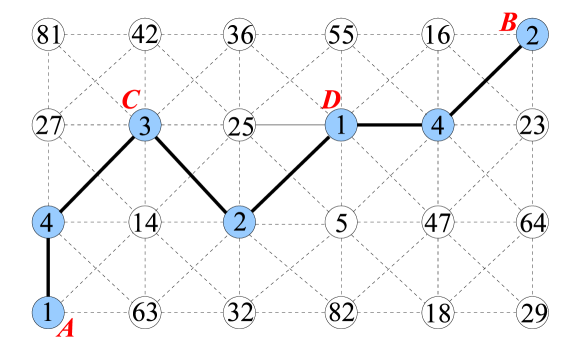
Figure 1: Discrete geodesic path on a 8-neighborhood graph. The points $C$ and $D$ belong to a geodesic path between $A$ et $B$. Therefore the geodesic distance between $C$ and $D$ is also known.

Using the property 1, when the geodesic distance between two points of the image is computed, the distances between all pairs of points along the associated geodesic path are known. Consequently, the distances array is filled faster using this redundancy.

In order to compute the distances between the points along the geodesic path, Bertelli et al. (2006) proposed to build a geodesic tree which has three kinds of nodes:

1. the root, which is the source point for a geodesic propagation. Its distance is null and it has no parents ;

2. the nodes, which are points having both parents and children ;

3. the leaves, which are points without children.

Starting from the leaves to the nodes (or the opposite), the distances between points belonging to the same geodesic path are easily computed.

The following additional property is very useful to compute all pairs of geodesic distances.

Property 2

The longer the geodesic paths are, the higher numbers of pairs of geodesic distances are computed.

In order to have the benefit of the property 2, Bertelli et al. (2006) have chosen as sources, of the geodesic propagations, random points in a spiral-like order: starting from the edges of the image and going to the center. Indeed, the points on the edges of the image tends to have longer geodesic paths than points located at the center. Consequently, we want to test their remark by comparing their method to some others.

In order to make this comparison, we measure the filling rates of the distances array $D$. For an image containing $N$ pixels, the distances array is a square matrix of size $N\times N=N^{2}$ elements. By symmetry, the number of geodesic paths to compute is equal to:

$$A=\frac{N^{2}-N}{2}$$ (11)

The number of computed paths $a$ is determined by counting the unfilled elements of the distances array $D$. In practice, it is useful to use a boolean matrix $D_{mrk}$, of size $N\times N$, with elements equal to 1 if the distance between the pixel located by the line number and the pixel located by the column number is computed, and 0 otherwise. By convention in the algorithm, we impose to each element of the diagonal of the boolean matrix to be equal to one, $\forall i$ $D_{mrk}(i,i)=1$, because the distance from one pixel to itself is equal to zero. Due to the symmetric properties of array $D$, the number of computed paths is equal to:

$$a = \frac{1}{2}\left[\left(\sum_{k=1}^{N}\sum_{l=1}^{N}D_{mrk}(k,l)\right)-trace(D_{mrk})\right]$$ (12)

$$= \frac{1}{2}\left[\left(\sum_{k=1}^{N}\sum_{l=1}^{N}D_{mrk}(k,l)\right)-N\right]$$

Consequently, the filling rate of the distances array is defined by:

$$\tau=\frac{a}{A}$$ (13)

The proportion of paths to compute for a given pixel $x_{i}$, is named the filling rate of the point $x_{i}$, and is defined by:

$$\tau(x_{i}) = \frac{\sum_{k=1}^{N}D_{mrk}(k,i)-D_{mrk}(i,i)}{N-1}$$ (14)

$$= \frac{\sum_{k=1}^{N}D_{mrk}(k,i)-1}{N-1}$$

When all the distances from one point to the others are computed, this point is said to be “filled”, i.e. $\tau(x_{i})=1$.

3 Introduction of new methods for fast computation of all pairs of geodesic distances

In the current section, we initially present Bertelli et al. (2006) method, named the “spiral method”, and then we introduce two new methods before making comparisons : 1) a geodesic extrema method and 2) a method based on the filling rate of all distances pairs array. The empirical comparisons are made on three different images of size $25\times 25$ pixels: “bumps”, “hairpin bend”, “random” (fig. 2).

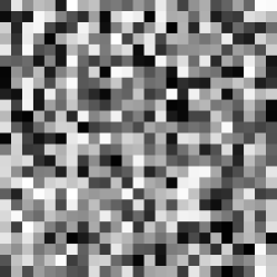
Image “bumps”	Image “hairpin bend”	Image “random”

Figure 2: Images of size $25\times 25$ pixels “bumps”, “hairpin bend” and “random” whose grey levels are between 1 and 255.

In order to use homogeneous measures for all methods, the Soille’s algorithm (Soille, 2013), called “geodesic time function” is used, with a discrete neighborhood of size $3\times 3$ pixels. In fact, we do not need an Euclidean geodesic algorithm to make this comparison study. The Euclidean version is described in (Soille, 1992) and improved in (Coeurjolly et al., 2004).

3.1 Spiral method

Bertelli et al. (2006) affirms that the source points of the geodesic propagations, with the longest paths, are in general situated on the borders of the image. As these points are useful to reduce the number of operations, the source points are chosen in a random way on concentric spiral turns of image pixels. A concentric spiral turn is a frame, of one pixel width, in which the top left corner is at position (1,1) or (2,2) or (3,3) or etc. The figure 3 gives an example. While not all the pixels of the spiral turns have been selected, we draw one pixel, among them, in a uniform random way ; otherwise we switch to the next spiral turn.

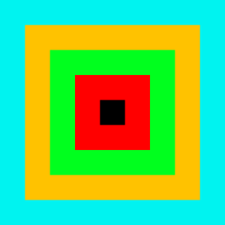
Figure 3: The spiral turns of an image $9\times 9$ pixels.

Table 1: Algorithm: Spiral method

1:  Given $D$ the distances array of size $N\times N$

2:  while  $D$ is not filled do

3:     Select the most exterior spiral turn not yet filled

4:     Determine $S$ the list of pixels of the spiral turn not yet filled

5:     while  $S$ is not empty  do

6:        Select a source point $s$ randomly in $S$

7:        Compute the geodesic tree from $s$

8:        Fill the distances array $D$

9:        Remove the points of $S$ which are filled

10:     end while

11:  end while

For each image, the filling rate is plotted versus the number of propagations (fig. 4). The number of propagations which are necessary to fill the distances array by the spiral method and the naive method are also given in this figure. The relative difference of the number of propagations of the spiral method compared to the number of propagations of the naive method is written $\Delta_{r}(naive)$. We notice that the spiral method reduces the number of propagations by a factor ranging between 13.4 % and 25.6 %, as compared to the naive one. Consequently, it is very useful to exploit the redundancy in the propagations by building a geodesic tree.

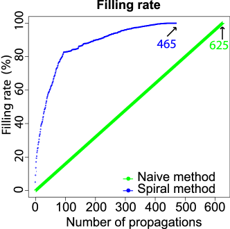
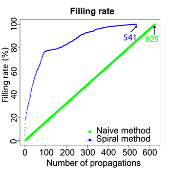
(a) “bumps”	(b) “hairpin bend”
$\Delta_{r}(naive)=25.6\%$	$\Delta_{r}(naive)=13.4\%$
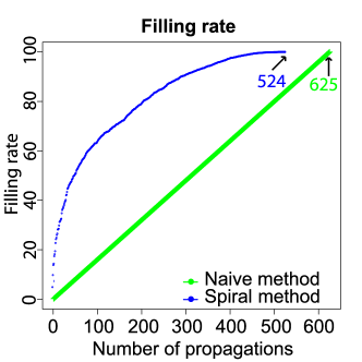
(c) “random”
$\Delta_{r}(naive)=16.2\%$

Figure 4: Comparison of the filling rates $\tau$ of the distances array, between the naive method (in green) and the spiral method (in blue) for the images “bumps”, “hairpin bend” and “random”. The relative differences $\Delta_{r}(naive)$ of the number of propagations of the spiral method compared to the number of propagations of the naive method are given on the bottom line.

3.2 Spiral method with repulsion

Two neighbours points have a high probability to have similar geodesic trees. Consequently, a first improvement of the spiral method is to introduced a repulsion distance between the points drawn randomly in a spiral like-order (algorithm of table 2). Several tests have shown us that a repulsion distance of three pixels on both sides of a source point gives the best filling rates.

These tests are empirical tests. In fact, several repulsion distances were tried and it has been noticed that the value of three pixels gives the best results in order to fill the array of distances. This value of three pixels is certainly related to the image size, because, generally, the farther the source points of the geodesic propagations are the faster the array of all pairs of geodesic distances is filled.

Table 2: Algorithm: Spiral method with repulsion

1:  Given $D$ the distances array of size $N\times N$

2:  Given $h$ the repulsion distance: $h$ $\leftarrow$ 3 pixels

3:  while  $D$ is not filled  do

4:     Select the most exterior spiral turn not yet filled

5:     Determine $S$ the list of pixels of the spiral turn not yet filled

6:     while  $S$ is not empty  do

7:        Select a source point $s$ randomly in $S$

8:        Remove in the list $S$ the two left points of $s$ and the two right points of $s$ if they are still in $S$

9:        Compute the geodesic tree from $s$

10:        Fill the array $D$

11:        Remove the points of $S$ which are filled

12:     end while

13:  end while

The figure 5, shows that the relative differences in the number of propagations necessary to fill the distances array are larger than 15 % for images “bumps” and “hairpin bend” and than 5.3 % for the image “random”. Therefore, the spiral method with the repulsion distance is faster than the spiral method to fill the distances array.

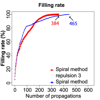
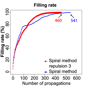
(a) “bumps”	(b) “hairpin bend”
$\Delta_{r}(spiral)=17.4\%$	$\Delta_{r}(spiral)=15.0\%$
$\Delta_{r}(naive)=38.6\%$	$\Delta_{r}(naive)=26.4\%$
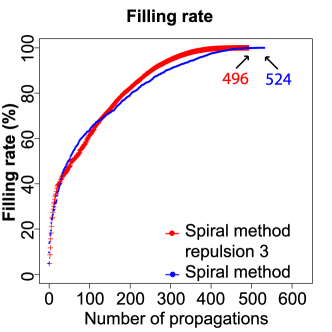
(c) “random”
$\Delta_{r}(spiral)=5.3\%$
$\Delta_{r}(naive)=20.6\%$

Figure 5: Comparison of the filling rates $\tau$ of the distances array, between the spiral method with repulsion (in red) and the spiral method (in blue) for the images “bumps”, “hairpin bend” and “random”. The relative differences $\Delta_{r}(spiral)$ (resp. $\Delta_{r}(naive)$) of the number of propagations of the spiral method with repulsion compared to the number of propagations of the spiral (resp. naive) method are given on the bottom lines.

3.3 Geodesic extrema method

As the longest geodesic paths are those which fill the most the distance array, we look for the geodesic extrema of the image. To compute the geodesic extrema of the image, we use two geodesic propagations:

• a first propagation starts from the edges of the image. Then we select one of the points $c$ with the longest distance from the edges. This point is called the geodesic centroid ;

• a second propagation from the geodesic centroid gives the farthest points from the centroid, i.e. the geodesic extrema of the image.

On the figure 6, which shows the results from these two propagations, we notice that the geodesic extrema are mainly on the edges of the image, which ascertains the motivation to use a spiral method.

Then the pixels are sorted by geodesic distance from the centroid into the list of geodesic extrema $Ext$. This list is used to choose the source points of the geodesic propagations. If several points have the same geodesic distance from the centroid, then the less filled is selected (algorithm of table 3).

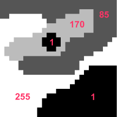
“bumps”	“hairpin bend”	“random”
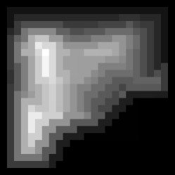
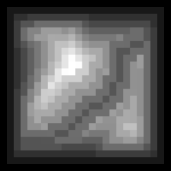
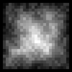
Geodesic distance from the edges of the image
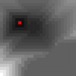
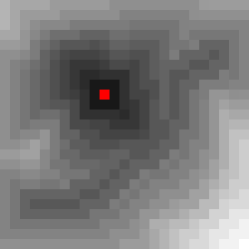
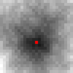
Geodesic distance from the centroid (red point)

Figure 6: Geodesic distance from the edges of the image (second line) and from the centroid in red (third line) for several images.

Table 3: Algorithm: Geodesic extrema method

1:  Given $D$ the distances array of size $N\times N$

2:  Compute the geodesic centroid $c$

3:  Compute the decreasing list of geodesic extrema $Ext$ whose first element $Ext[1]$ is the greatest geodesic extrema not yet filled

4:  Initialise to zero, the list, of size $N$, of the filling rate of points $\tau$.

5:  while  $D$ is not filled do

6:        $B$ $\leftarrow$ $\{x\in Ext|d_{geo}(x,c)=d_{geo}(Ext[1],c)\}$

7:        $s$ $\leftarrow$ $x$

8:        Compute the geodesic tree from $s$

9:        Fill the distances array $D$

10:        Remove the points of the list $Ext$ which are filled

11:        Update the list of filling rates $\tau$

12:  end while

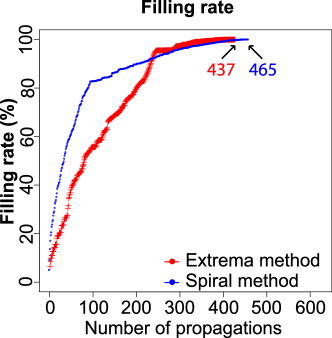
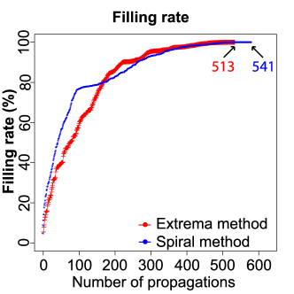
(a) “bumps”	(b) “hairpin bend”
$\Delta_{r}(spiral)=6.0\%$	$\Delta_{r}(spiral)=5.2\%$
$\Delta_{r}(naive)=30.1\%$	$\Delta_{r}(naive)=17.9\%$
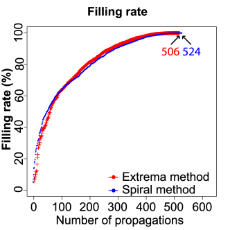
(c) “random”
$\Delta_{r}(spiral)=3.4\%$
$\Delta_{r}(naive)=19.0\%$

Figure 7: Comparison of the filling rates $\tau$ of the distances array, between the geodesic extrema method (in red) and the spiral method (in blue) for the images “bumps”, “hairpin bend” and “random”. The relative differences $\Delta_{r}(spiral)$ (resp. $\Delta_{r}(naive)$) of the number of propagations of the the geodesic extrema method compared to the number of propagations of the spiral (resp. naive) method are on the bottom lines.

The filling rates of the spiral method and the geodesic extrema method versus the number of propagations are plotted for each image (fig. 7). We notice that the filling rates of the geodesic extrema method are at the beginning inferior or similar to these of the spiral method. However, at the end the filling rates of the geodesic extrema method are better than these of the spiral method. In fact, we are looking for an approach filling totally the distances array in the fastest way. As the number of propagations of the geodesic extrema method necessary to fill the distances array are lower than in the spiral method, the geodesic extrema method fills faster the distances array than the spiral method.

In order to get an exact comparison it is necessary to generate two propagations, corresponding to the determination of the geodesic extrema, to the number of propagations necessary to fill the distances array. Even, with this modification, the extrema method fills the distances array faster than the spiral method (the relative differences $\Delta_{r}(spiral)$ are between 3.4 % and 6 %).

3.4 Method based on the filling rate of the distances array

In place of selecting the source points from their distance from the geodesic centroid propagation, we select first the less filled points. To this aim, after each geodesic propagation the filling rate is computed for each point. Then the less filled point is selected as a source of the propagation. If several points are among the less filled, then the greatest geodesic extrema is chosen among these points (algorithm of table 4).

Table 4: Algorithm: Method based on the filling rate of the distances array

1:  Given $D$ the distances array of size $N\times N$

2:  Compute the decreasing list of geodesic extrema $Ext$

3:  Initialise to zero, the list, of size $N$, of the filling rate of points $\tau$.

4:  while  $D$ is not filled  do

5:     $B$ $\leftarrow$ $\{\operatorname*{argmin}_{x\in E}\tau[x]\}$

6:     if  $Card\{B\}>1$ then

7:        $s$ $\leftarrow$ $\operatorname*{argmin}_{x\in B}Ext[x]$

8:     else

9:        $s$ $\leftarrow$ $\operatorname*{argmin}_{x\in E}\tau[x]$

10:     end if

11:     Compute the geodesic tree from $s$

12:     Fill the distances array $D$

13:     Remove the points of the list $Ext$ which are filled

14:     Update the list of filling rates $\tau$

15:  end while

As for the geodesic extrema method, we compare the filling rates of the method based on the filling rate of the distances array and the spiral method versus the number of propagations (fig. 8). We notice that the method based on the filling rate of $D$ reduces of 32.3 % the number of propagations of the spiral method on the image “bumps” and 18.7 % on the image “hairpin bend”. Consequently this method fills faster the distances array than the spiral method. Even for the image “random” the method based on the filling rate of $D$ still improves the spiral method of 2.7 %. However it is not very common to compute all pairs of geodesic distances on a strong unstructured image such as the “random” one.

By comparison to the naive approach, the method based on the filling rate of $D$ reduces the number of propagations by a 49.6 % rate (resp. 29.6 %) on the image “bumps” (resp. “hairpin bend”).

As for the previous method, in order to get an exact comparison, it is necessary to add two propagations, corresponding to the determination of the geodesic extrema, to the number of propagations necessary to fill the distances array. Even, with this modification, the number of propagations necessary to fill the distances array is still lower for the method based on the filling rate of $D$.

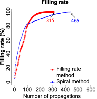
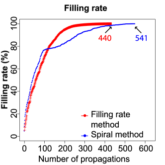
(a) “bumps”	(b) “hairpin bend”
$\Delta_{r}(spiral)=32.3\%$	$\Delta_{r}(spiral)=18.7\%$
$\Delta_{r}(naive)=49.6\%$	$\Delta_{r}(naive)=29.6\%$
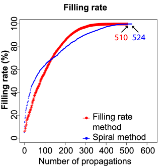
(c) “random”
$\Delta_{r}(spiral)=2.7\%$
$\Delta_{r}(naive)=18.4\%$

Figure 8: Comparison of the filling rates $\tau$ of the distances array, between the method based on the filling rate of the distances array (in red) and the spiral method (in blue) for the images “bumps”, “hairpin bend” and “random”. The relative differences $\Delta_{r}(spiral)$ (resp. $\Delta_{r}(naive)$) of the number of propagations of the method based on the filling rate compared to the number of propagations of the spiral (resp. naive) method are given on the bottom lines.

4 Discussion

After having presented and tested several methods to fill the distances array, we have compared them for the three test images “bumps”, “hairpin bend” and “random” on the figure 9 and in the table 5. For the images “bumps” and “hairpin bend”, the method based on the filling rate of the distances array is faster than the other algorithms. For the “random image” (an extreme case presenting no texture) the methods introduced here give similar results, since the relative difference between the maximum number of propagations is less than 2.7 %. Therefore, we conclude that the method based on the filling rate of the distances array is the best one to calculate the array of all pairs of distances. According to their performances, the others are ranked in the following order: 1) the spiral method with repulsion distance, 2) the geodesic extrema method and 3) the spiral method of Bertelli et al. (2006).

Moreover, we have shown that the method based on the filling rate of $D$ reduces the number of operations between 19 % and 32 %, as compared to the spiral approach and between 30 % and 50 %, as compared to the naive method, on standard images. Even on “random” image the improvements is of 3 % (resp 18 %) compared to the spiral (resp. naive) method.

Consequently, the filling rate of the distances array, combined with the geodesic extrema when several points have the minimum filling rate, seems to be the best criterion to fill efficiently the distances array.

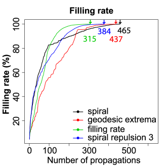
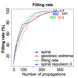
(a) “bumps”	(b) “hairpin bend”
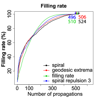
(c) “random”

Figure 9: Comparison of the filling rates, of the array of distances, for the methods: spiral, geodesic extrema, the method based on the filling and the spiral method with a repulsion distance of 3 pixels for the images “bumps”, “hairpin bend” and “random”.

	Spiral	spiral	geodesic	filling
$\Delta_{r}(naive)$	method	method with	extrema	rate
		repulsion	method	method
“Bumps”	25.6 %	38.6 %	30.1 %	49.6 %
“Hairpin bend”	13.4 %	26.4 %	17.9 %	29.6 %
“Random”	16.2 %	20.6 %	19.0 %	18.4 %

(a)
spiral geodesic filling $\Delta_{r}(spiral)$ method with extrema rate repulsion method method “Bumps” 17.4 % 6.0 % 32.3 % “Hairpin bend” 15.0 % 5.2 % 18.7 % “Random” 5.3 % 3.4 % 2.7 %
(b)

Table 5: Relative difference values of filling rates (a) between the different methods and the naive approach, or (b) between the different methods and the spiral approach. For each image is given in bold the best relative difference value.

5 Conclusion

From a comparison between different approaches, it turns out that a method based on the optimization of the filling rate of the distances array is the most efficient to compute the geodesic distances between all pairs of pixels in an image.

Besides, in the current paper, we have shown our results on grey images. They can be directly extended to hyperspectral images using appropriate pseudo-metrics (Noyel et al., 2007a). This can be a useful step for a subsequent clustering by kernel methods or data reduction approaches on multivariate images.

The main motivation for our developments is the computation of all pairs of geodesic distances for the pixels of an image, which is usually a graph of thousands of vertices arranged spatially. Nevertheless, our approach is valid on more general graphs, than those associated to bitmap images, after determining the “boundary vertices” of the graph, since then, the computation of the geodesic centre (and the geodesic extremities) of a graph can be obtained by a first propagation from the “boundary vertices”. The “boundary vertices” can be defined, for instance, as the vertices having less neighbouring vertices than the average number of connectivity in the graph.

References

- Bertelli and Manjunath (2007) Bertelli L, Manjunath BS (2007). Edge preserving filters using geodesic distances on weighted orthogonal domains. In: 2007 IEEE International Conference on Image Processing, vol. 1.
- Bertelli et al. (2006) Bertelli L, Sumengen B, Manjunath BS (2006). Redundancy in all pairs fast marching method. In: 2006 IEEE International Conference on Image Processing.
- Coeurjolly et al. (2004) Coeurjolly D, Miguet S, Tougne L (2004). 2d and 3d visibility in discrete geometry: an application to discrete geodesic paths. Pattern Recognition Letters 25:561 – 570. Discrete Geometry for Computer Imagery (DGCI’2002).
- Grazzini and Soille (2009) Grazzini J, Soille P (2009). Edge-preserving smoothing using a similarity measure in adaptive geodesic neighbourhoods. Pattern Recognition 42:2306 – 2316. Selected papers from the 14th IAPR International Conference on Discrete Geometry for Computer Imagery 2008.
- Lantuejoul and Maisonneuve (1984) Lantuejoul C, Maisonneuve F (1984). Geodesic methods in quantitative image analysis. Pattern Recognition 17:177 – 187.
- Lerallut et al. (2007) Lerallut R, Decencière E, Meyer F (2007). Image filtering using morphological amoebas. Image and Vision Computing 25:395 – 404. International Symposium on Mathematical Morphology 2005.
- Mohan et al. (2007) Mohan A, Sapiro G, Bosch E (2007). Spatially coherent nonlinear dimensionality reduction and segmentation of hyperspectral images. IEEE Geoscience and Remote Sensing Letters 4:206–10.
- Noyel (2008) Noyel G (2008). Filtering, dimensionality reduction, classification and morphological segmentation of hyperspectral images. Theses, École Nationale Supérieure des Mines de Paris.
- Noyel et al. (2007a) Noyel G, Angulo J, Jeulin D (2007a). Morphological segmentation of hyperspectral images. Image Analysis Stereology 26:101–9.
- Noyel et al. (2007b) Noyel G, Angulo J, Jeulin D (2007b). On distances, paths and connections for hyperspectral image segmentation. In: Banon G, et al., eds., International Symposium on Mathematical Morphology, vol. 1. Rio de Janeiro, Brazil: Instituto Nacional de Pesquisas Espaciais (INPE). ISBN 978-85-17-00035-5.
- Sethian (1999) Sethian J (1999). Level Set Methods and Fast Marching Methods: Evolving Interfaces in Computational Geometry, Fluid Mechanics, Computer Vision, and Materials Science. Cambridge Monographs on Applied and Computational Mathematics. Cambridge University Press.
- Sethian (1996) Sethian JA (1996). A fast marching level set method for monotonically advancing fronts. Proceedings of the National Academy of Sciences 93:1591–5.
- Soille (1991) Soille P (1991). Spatial distributions from contour lines: An efficient methodology based on distance transformations. Journal of Visual Communication and Image Representation 2:138 – 150.
- Soille (1992) Soille P (1992). Morphologie Mathématique: du relief à la dimensionalité - algorithmes et méthodes. Ph.D. thesis, Sciences Agronomiques, Université Catholique de Louvain.
- Soille (1994) Soille P (1994). Generalized geodesy via geodesic time. Pattern Recognition Letters 15:1235 – 1240.
- Soille (2013) Soille P (2013). Morphological Image Analysis: Principles and Applications. Springer Berlin Heidelberg, 2nd ed.
- Tenenbaum (1998) Tenenbaum JB (1998). Mapping a manifold of perceptual observations. In: Advances in Neural Information Processing Systems 10. MIT Press.
- Tenenbaum et al. (2000) Tenenbaum JB, Silva Vd, Langford JC (2000). A global geometric framework for nonlinear dimensionality reduction. Science 290:2319–23.