Viscoelastic flows of Maxwell fluids
with conservation laws

Abstract

We consider multi-dimensional extensions of Maxwell’s seminal rheological equation for 1D viscoelastic flows. We aim at a causal model for compressible flows, defined by semi-group solutions given initial conditions, and such that perturbations propagates at finite speed.

We propose a symmetric hyperbolic system of conservation laws that contains the Upper-Convected Maxwell (UCM) equation as causal model. The system is an extension of polyconvex elastodynamics, with an additional material metric variable that relaxes to model viscous effects. Interestingly, the framework could also cover other rheological equations, depending on the chosen relaxation limit for the material metric variable.

We propose to apply the new system to incompressible free-surface gravity flows in the shallow-water regime, when causality is important. The system reduces to a viscoelastic extension of Saint-Venant 2D shallow-water system that is symmetric-hyperbolic and that encompasses our previous viscoelastic extensions of Saint-Venant proposed with F. Bouchut.

1 Introduction

In 1867, when viscosity was already an important concept to model friction within fluid flows at the human scale following Poisson’s theory of friction [53], Maxwell introduced a seminal relaxation equation for the rheology of one-dimensional (1D) flows where viscosity is defined from elasticity and a characteristic time [46]. The viscoelastic model of Maxwell is long known as an interesting model for 1D flows: given initial conditions, fluid motions are well-defined [30] that are genuinely causal, i.e. causal and local in particular.

By contrast, nowadays, viscosity is often introduced in continuum mechanics as a material parameter into the momentum balance of motions described in spatial coordinates [15]. It still allows to define causal viscous flows as semi-group solutions to Cauchy problems. However, it uses diffusive Partial Differential Equations (PDEs) like the celebrated Navier-Stokes equations [41], and the latter viscous flows do not satisfy the desirable principle of locality (i.e. motions are not genuinely causal) because information propagates at infinite speed. Now, locality is important in geophysics e.g. when unstationary processes associated with internal friction obviously have a local character (the migration of suspended particles, the production of turbulent energy…).

In this work, to model viscosity in fluid flows, we follow Maxwell’s approach and we look for a good (hyperbolic) viscoelastic model.

Many viscoelastic models have been proposed after Maxwell, in particular to explain non-Newtonian flows of polymeric rubber-like liquids after [18] that are mostly steady. For multi-dimensional flows, there is now a consensus about the need for a rheological equation with objective derivatives, like the famous Upper-Convected Maxwell (UCM) equation. But flow models with UCM are usually formulated as quasilinear systems without more structure; and solutions to Cauchy problems have remained difficult to analyze or simulate beyond 1D. In practice, the UCM models – mostly used for incompressible flows – are often modified with an additional “background viscosity” (equiv. a retardation time) e.g. as in the Oldroyd-B model, which spoils the local character of Maxwell’s model. See Section 2 for more details about standard viscoelastic models.

In this work, we propose the first formulation of the compressible UCM model as a symmetric-hyperbolic system of conservation laws in Section 3.

Starting with the elastodynamics system like the K-BKZ theory for viscoelastic models [33, 34, 2, 3], a new system of physically-meaningful conservation laws is proposed for the compressible UCM model in section 3.1.

In section 3.2, it is then proved that the system is symmetric-hyperbolic, using conservative variables adequate for the application of Godunov-Mock theorem. Recall that symmetric-hyperbolic systems of conservation laws are essential to the analysis and to the numerical simulation of solutions to quasilinear systems [1], and to polyconvex elastodynamics in particular [16, 58, 7].

The new system is not simply a sound mathematical framework for the viscoelastic models under development [42]. It is also one particular viscoelastic case in a class of mathematically-sound models that unifies the hyperelastic solids with viscous fluids.

In section 3.3, we show that the new system has not only a physical interpretation as one extension of the polyconvex elastodynamics system (usually modelling solids), but also one particular extension towards fluids, that uses an additional material metric variable like other well-known extensions (e.g. the elastoplastic systems). That latter interpretation shows the potentialities of the new symmetric-hyperbolic system of conservation laws, to soundly unify the solid and fluid dynamics of various materials.

Unifying fluid and solid dynamics has of course been the goal of many previous works in the literature, and it is not the aim of the present work to review and compare them with our new system. Here, unification is simply mentioned as a potentiality of our new system. Let us nevertheless mention the recent work [51]. As for unification, that work is the only one we are aware of which, like ours, first looks for a symmetric-hyperbolic system of conservation laws extending polyconvex elastodynamics to viscoelastic Maxwell fluids. In comparison with [51], we extend polyconvex elastodynamics to a hyperbolic quasilinear system with a different structure, using a different additional variable.

Last, we believe our new system will have very useful applications in the shallow-water regime, to model free-surface gravity flows with viscosity.

In Section 4, we precisely show how our new system can be reduced to a symmetric-hyperbolic system of 2D conservation laws that is a physically-meaningful viscoelastic extension of Saint-Venant models. The new 2D system encompasses our former viscoelastic extensions of Saint-Venant models with F. Bouchut [10, 11, 12], without a conservative formulation in 2D.

Developping 2D shallow-water models for free-surface flows with large vertical vortices and viscous dissipation has also been the goal of many previous works in the literature, see [22, 11] and references therein. Again, it is not the goal of the present article to review and compare those numerous 2D works with ours. Here, we simply mention an important application of our new 3D UCM system, which delivers a symmetric-hyperbolic system of 2D conservation laws in contrast to [23] and our former works [11, 12] e.g., see details in Section 4.

2 Viscoelastic flows in continuum mechanics

First recall standard viscoelastic constitutive assumptions to model smooth compressible material fluid motions (equiv. flows) in continuum mechanics setting.

2.1 Continuum mechanics needs constitutive assumptions

Continuum mechanics aims at modelling the motions of “matter” as flows of “continuous bodies” at the human scale (unlike “discrete particles” at the molecular scale). A prerequisite is the definition of material bodies and their flows.

The classical theory considers bodies $\mathcal{B}$ that are Riemannian manifolds, and flows that are collections of “configurations” i.e. mappings $\boldsymbol{\phi}_{t}(\mathcal{B})$ indexed by time $t\in\mathbb{R}$ into the Euclidean ambiant space [44]. For future reference, recall that on bodies $\mathcal{B}$ with a coordinate system $\{a^{\alpha}\}$ and a material (or body) metric defined by a positive symmetric 2-tensor $G_{\alpha\beta}\in S^{+}(\mathbb{R}^{d\times d})$ ($d=2,3$), $\operatorname{div}_{\boldsymbol{a}}\boldsymbol{v}=\partial_{\alpha}(\sqrt{|G|}v^{\alpha\beta\ldots})/\sqrt{|G|}$ for $\boldsymbol{v}(\boldsymbol{a})=v^{\alpha\beta\ldots}\boldsymbol{e}_{\alpha}\otimes\boldsymbol{e}_{\beta}\dots$ is well-defined when $G_{\alpha\beta}\in S^{++}(\mathbb{R}^{d\times d})$ i.e. the determinant is stricly positive $|G_{\alpha\beta}|>0$, and an inverse metric $G_{\alpha\beta}G^{\beta\gamma}=\delta_{\alpha\gamma}$ exists – $\delta_{\alpha\gamma}$ denoting Kronecker’s symbol –.

Next, one establishes a precise description of bodies motions i.e. “flows” using axioms and assumptions. Viscoelastic flows arise from particular constitutive assumptions, see section 2.3. But let us first recall the continuum mechanics setting and simpler consitutive equations (some notions need to be assumed though, like those in quotes “…”, and we refer to [16, 44, 60] for more details).

Given a force field $\boldsymbol{f}$ in the Euclidean ambiant space with a coordinate system $\{x^{i}\}$, one assumes a Galilean frame-invariant balance of total energy $E\geq 0$ holds as follows for bodies, with $R$ the heat supplied during the process:

$$\partial_{t}(E\circ\boldsymbol{\phi}_{t})=\operatorname{div}_{\boldsymbol{a}}(S^{i\alpha}\partial_{t}\phi^{i}_{t})+\partial_{t}\phi^{i}_{t}(f^{i}\circ\boldsymbol{\phi}_{t})+R\,.$$ (1)

Then, bodies are characterized by a mass-density $\hat{\rho}(\boldsymbol{a})\geq 0$, and their motions $\boldsymbol{\phi}_{t}:\boldsymbol{a}\in\mathcal{B}\rightarrow\boldsymbol{x}=\boldsymbol{\phi}_{t}(\boldsymbol{a})\in\mathbb{R}^{d}$ ($d=2,3$) satisfy the momentum balance:

$$\hat{\rho}(\partial^{2}_{tt}\boldsymbol{\phi}_{t})=\operatorname{div}_{\boldsymbol{a}}\boldsymbol{S}+\hat{\rho}(\boldsymbol{f}\circ\boldsymbol{\phi}_{t})$$ (2)

where $\boldsymbol{S}$ is the (first) Piola-Kirchoff stress tensor, $S^{i\alpha}$ in coordinates. For non-polar bodies, it holds $S^{i\alpha}\partial_{\alpha}\phi^{j}=S^{j\alpha}\partial_{\alpha}\phi^{i}$ and, on introducing $r\circ\boldsymbol{\phi}_{t}=R/\hat{\rho}$,

$$\hat{\rho}(\partial_{t}e\circ\boldsymbol{\phi}_{t})-S^{i\alpha}\partial^{2}_{t\alpha}\phi^{i}_{t}=\hat{\rho}(r\circ\boldsymbol{\phi}_{t})$$ (3)

where $e\circ\boldsymbol{\phi}_{t}:=E\circ\boldsymbol{\phi}_{t}/\hat{\rho}-\frac{1}{2}|\partial_{t}\boldsymbol{\phi}_{t}|^{2}$ is the internal energy. Note that we assume adiabatic processes (i.e. no heat flux within bodies, which are assumed heat insulators), and we use Einstein summation convention for repeated indices.

Next, if constitutive assumptions specify $e$ as a function of $\partial_{\alpha}\phi^{i}_{t}$ – thus also $\boldsymbol{S}$ by (3) –, motions $\boldsymbol{\phi}_{t}$ can be defined as solutions to (2) for $t\in[0,T)$ given $\phi_{t=0}=\phi_{0}$. Some constitutive assumptions and well-defined motions have shown the practical interest of the theory for applications to various materials, see e.g. [39, 7]. But specifying constitutive assumptions that are both mathematically and physically meaningful is a difficult task since the beginning of the theory. Despite many rationalization efforts guided by mathematical soundness, we are not aware of a definitive approach to model particular real materials (many practical constitutive assumptions exist, scattered in a vast literature). We recall standard constitutive assumptions for viscoelastic fluids in section 2.3.

In section 2.2, we first recall fundamental constitutive assumptions for elastic and viscous material bodies in the “solid” or “fluid” states, when $e$ is function of $\partial_{\alpha}\phi^{i}_{t}$ or $|\partial_{\alpha}\phi^{i}_{t}|$. Viscoelasticity arises as a unifying concept in between. We consider smooth motions $\boldsymbol{\phi}_{t}$, diffeomorphisms with inverse $\boldsymbol{\phi}_{t}^{-1}$, and we denote:

• $F^{i}_{\alpha}:=\partial_{\alpha}\phi^{i}_{t}\circ\boldsymbol{\phi}_{t}^{-1}$ the deformation gradient in component form given two coordinates systems $\{x^{i}\}$ and $\{a^{\alpha}\}$, i.e. the matrix representation of the tensor $\boldsymbol{F}=F^{i}_{\alpha}\boldsymbol{e}_{i}\otimes\boldsymbol{e}_{\alpha}$ with rows labelled by a Roman letter like $i,j,k\dots$ to precise coordinates in the spatial frame and with columns labelled by a Greek letter $\alpha,\beta,\gamma,\dots$ to precise coordinates in the material frame

• $|F^{i}_{\alpha}|$ the determinant of $F^{i}_{\alpha}$, also sometimes denoted $|\boldsymbol{F}|$

• $C^{\alpha}_{i}$ the cofactor matrix (or transpose adjugate) of $F^{i}_{\alpha}$

• $u^{i}:=\partial_{t}\phi^{i}_{t}\circ\boldsymbol{\phi}_{t}^{-1}$ the velocity

• $D(u)^{ij}:=\frac{1}{2}\left(\partial_{i}u^{j}+\partial_{j}u^{i}\right)$ the strain-rate tensor

• $\operatorname{div}\boldsymbol{u}=\partial_{i}u^{i}$ the Euclidean divergence for a vector field $\boldsymbol{u}$ and

• $\delta$ the identity tensor compatible with the Kronecker symbol notation in coordinates so $\delta_{i}^{j}=|F^{i}_{\alpha}|^{-1}F^{j}_{\alpha}C^{\alpha}_{i}$ for instance.

We classically assume that (1)–(2) are the Euler-Lagrange equations of a variational principle for a Lagrangian density $\hat{\rho}\left(\frac{1}{2}|\partial_{t}\boldsymbol{\phi}_{t}|^{2}-e\circ\boldsymbol{\phi}_{t}\right)$ with $e$ a function of $\partial_{\alpha}\phi^{i}_{t}$, [44], and $G_{\alpha\beta}=\delta_{\alpha\beta}$ for simplicity. Then, $\boldsymbol{S}$ is a function of $F_{\alpha}^{i}\circ\boldsymbol{\phi}_{t}$ i.e.

$$S^{i\alpha}=\hat{\rho}\partial_{F^{i}_{\alpha}}e$$ (4)

so (3) holds with $r=0$. And (2) rewrites within a system of conservation laws:

$$\partial_{t}\left(\hat{\rho}\>u^{i}\circ\boldsymbol{\phi}_{t}\right)-\partial_{\alpha}S^{i\alpha}=\hat{\rho}f^{i}$$ (5)

$$\partial_{t}\left(F^{i}_{\alpha}\circ\boldsymbol{\phi}_{t}\right)-\partial_{\alpha}\left(u^{i}\circ\boldsymbol{\phi}_{t}\right)=0$$

$$\partial_{t}\left(|F^{i}_{\alpha}|\circ\boldsymbol{\phi}_{t}\right)-\partial_{\alpha}\left(C^{\alpha}_{j}\circ\boldsymbol{\phi}_{t}\>u^{j}\circ\boldsymbol{\phi}_{t}\right)=0$$

that fully defines causal motions in the so-called material (or Lagrangian) description as semi-group solutions, possibly after adding (6) to (5) when $d=3$

$$\partial_{t}\left(C^{\alpha}_{i}\circ\boldsymbol{\phi}_{t}\right)+\sigma_{ijk}\sigma_{\alpha\beta\gamma}\partial_{\beta}\left(F^{j}_{\gamma}\circ\boldsymbol{\phi}_{t}\>u^{k}\circ\boldsymbol{\phi}_{t}\right)=0$$ (6)

where $C^{\alpha}_{i}=\sigma_{ijk}\sigma_{\alpha\beta\gamma}F^{j}_{\beta}F^{k}_{\gamma}$, and $\sigma$ is Levi-Civita’s symbol – so it holds e.g.

$$|F^{i}_{\alpha}|=\sigma_{ij}\sigma_{\alpha\beta}F^{i}_{\alpha}F^{j}_{\beta}\qquad C^{\alpha}_{i}=|F^{i}_{\alpha}|\sigma_{ij}\sigma_{\alpha\beta}F^{j}_{\beta}$$

when $d=2$. Moreover, when $\hat{\rho}$ is constant, smooth motions with a material (or Lagrangian) description also have a spatial (or Eulerian) description:

$$\partial_{t}\left(\rho u^{i}\right)+\partial_{j}\left(\rho u^{j}u^{i}-\sigma^{ij}\right)=\rho f^{i}$$ (7)

$$\partial_{t}\left(\rho F^{i}_{\alpha}\right)+\partial_{j}\left(\rho u^{j}F^{i}_{\alpha}-\rho F^{j}_{\alpha}u^{i}\right)=0$$

$$\partial_{t}\rho+\partial_{j}\left(\rho u^{j}\right)=0$$

with Cauchy stress $\sigma^{ij}:=|F^{i}_{\alpha}|^{-1}F^{j}_{\alpha}S^{i\alpha}\circ\boldsymbol{\phi}_{t}^{-1}$ function of $F^{i}_{\alpha}$, and $\rho:=|F^{i}_{\alpha}|^{-1}\hat{\rho}$ [58], possibly complemented when $d=3$ by

$$\partial_{t}\left(\rho C^{\alpha}_{i}\right)+\partial_{j}\left(\rho u^{j}C^{\alpha}_{i}\right)+\sigma_{ijk}\sigma_{\alpha\beta\gamma}\partial_{l}\left(|F^{i}_{\alpha}|^{-1}F^{l}_{\beta}F^{j}_{\gamma}u^{k}\right)=0\,.$$ (8)

The Lagrangian and Eulerian descriptions of smooth motions are equivalent as long as the following Piola’s identities hold [58]:

$$\partial_{j}(|F^{i}_{\alpha}|^{-1}F^{j}_{\alpha})=0\quad\forall\>i=1\ldots d.$$ (9)

2.2 Constitutive assumptions for elastic bodies and fluids

Elastic motions

have been considered since the beginnings of continuum mechanics for “solids” [60, 45]. Some elastic constitutive assumptions efficiently summarize the molecular structure of matter at a human scale and are useful to predict real solid behaviours. In particular, smooth motions of hyperelastic materials with an energy $e(F^{i}_{\alpha}\circ\boldsymbol{\phi}_{t})$ can be well defined when $r=0$ as solutions to (a Cauchy problem for) either the second-order equation (2) [29], or a first-order system of conservation laws: (5) in material coordinates, or (7) in spatial coordinates, e.g. when $e$ is polyconvex and both are symmetric-hyperbolic [58].

Postulating indifference to Galilean changes of spatial frames as usual in classical physics requires that $e$ is function of $F^{i}_{\alpha}$ through the right Cauchy-Green deformation tensor $F^{k}_{\alpha}F^{k}_{\beta}$. Then, for homogeneous isotropic bodies with $G^{\alpha\beta}=\delta^{\alpha\beta}$ Euclidean, a useful polyconvex energy is the neo-Hookean

$$e(F^{k}_{\alpha}F^{k}_{\alpha}):=\frac{\mu}{2}(F^{k}_{\alpha}F^{k}_{\alpha}-d)$$ (10)

with both molecular and phenomenological justifications [24].

The neo-Hookean model is simplistic, but it is already quantitativaly useful for practical applications. Moreover, it has many refinements. For instance, the neo-Hookean model cannot capture volumetric changes observed simultaneously with elongation. But one can either use the model along with the incompressibility constraint $|F^{i}_{\alpha}|=1$ (if relevant) as a remedy. Or one can add a compressible term function of $|F^{i}_{\alpha}|$ in the energy (10) that preserves polyconvexity.

Non-reversible motions with $r\neq 0$ can moreover be considered when $e$ is a function of $F^{i}_{\alpha}$ and entropy $\eta$ such that it holds for some dissipation $D\geq 0$:

$$r\circ\boldsymbol{\phi}_{t}=(\theta\circ\boldsymbol{\phi}_{t})\partial_{t}(\eta\circ\boldsymbol{\phi}_{t})-D\circ\boldsymbol{\phi}_{t}\,.$$ (11)

Usual elongations with volumetric changes are indeed non-reversible, with heat exchanges $r\neq 0$; (11) means that the heat supply may be either dissipated by irreversible processes (“inelasticities”) or compensated for by variations in the body state (through entropy). Using (11) as an additional constitutive assumption leads one to introduce the temperature $\theta=-\partial_{\eta}e$ [15]. Then, further constitutive assumptions about inelasticities and $D$ allow to close (2) (or (5), or (7)) complemented by (3)–(11) when $r\neq 0$. For instance, smooth isentropic motions such that $\partial_{t}(\eta\circ\boldsymbol{\phi}_{t})=0$ can be defined for polyconvex hyperelastic bodies with $e$ jointly convex in $F^{i}_{\alpha}$ and $\eta$, as well as non-smooth motions like 1D shocks using the inequality associated with (3)–(11) [16].

Thermo-elastic models in fact use the Helmholtz free energy $\psi=e-\theta\eta$ as a function of $\theta$ more often than $e$ as a function of $\eta$, with a constitutive assumption precising the temperature evolution rather than the entropy evolution. Then

$$\hat{\rho}\left((\eta\circ\boldsymbol{\phi}_{t})\partial_{t}(\theta\circ\boldsymbol{\phi}_{t})+\partial_{t}(\psi\circ\boldsymbol{\phi}_{t})\right)-S^{i\alpha}\partial_{\alpha}(u^{i}\circ\boldsymbol{\phi}_{t})=-\hat{\rho}D\circ\boldsymbol{\phi}_{t}$$ (12)

complements (2) (or (5), or (7)) rather than (3)–(11). It allows one to define (smooth and non-smooth) isothermal motions for polyconvex hyperelastic bodies when $\psi$ is jointly convex in $F^{i}_{\alpha}$ and $\theta$ using $\eta=-\partial_{\theta}\psi$ and $S^{i\alpha}=\hat{\rho}\partial_{F^{i}_{\alpha}}\psi$.

Non-reversible motions however need a more accurate description in many applications. And it remains an active research field how to specify inelasticities, especially over a range of temperatures where the material properties change a lot (throughout phase transitions) and for large deformations of flowing bodies when the fluidity concept enters [4]. Viscoelasticity is one example of inelasticity. This will be very clear in Section 3 with our new UCM system. We show in section 3.3 that the UCM model is only one viscoelastic instance within a large class of mathematically-sound models with inelasticities. But first, let us recall a standard introduction of viscosity alone, without elasticity, as a constitutive assumption for imperfections in irreversible flows of fluids.

Fluid flows

have long been considered in continuum mechanics. The molecular structure of fluids is more difficult to summarize than that of solids, because they are much more deformable. Useful constitutive assumptions for simple enough fluid materials have been proposed – though usually without a clear link to solids, the fluid-solid transition being a well-identified difficulty [4].

A useful constitutive law for “perfect” fluids is the polytropic law

$$e(\rho):=\frac{C_{0}}{\gamma-1}\rho^{\gamma-1}.$$ (13)

Smooth motions can be defined with (13) in the reduced spatial description

$$\partial_{t}\rho+\partial_{i}(u^{i}\rho)=0$$ (14)

$$\rho\left(\partial_{t}u^{i}+u^{j}\partial_{j}u^{i}\right)-\partial_{j}\>\sigma^{ij}=\rho f^{i}$$

where the Cauchy stress tensor reduces to a pure pressure $p\equiv-\partial_{\rho^{-1}}e=C_{0}\rho^{\gamma}$

$$\sigma^{ij}=-p\>\delta_{ij}\,.$$ (15)

The system (14) is indeed symmetric-hyperbolic, and it is useful e.g. for the dynamics of simple (monoatomic) gases. But note that (14) is strictly contained in the Eulerian system (7), and motions are not equivalently described by the larger Lagrangian system (5) which is not symmetric hyperbolic.

Non-smooth irreversible motions can also be considered with (14) complemented by (11) and an entropy variable $\eta$. When $e$ is (jointly) convex in $\rho$ and $\eta$, one can consider isentropic motions through weak solutions, and define univoque 1D shocks [43]. Isomorphocally, one can define isothermal motions using Helmholtz free energy $\psi$, the spatial version of (12)

$$\rho\left(\eta(\partial_{t}+u^{i}\partial_{i})\theta+(\partial_{t}+u^{i}\partial_{i})\psi\right)=-\rho D+\sigma^{ij}\partial_{j}u^{i}$$ (16)

and a temperature variable $\theta$. However, more constitutive assumptions are often needed to precisely describe irreversible fluid motions, like the vortices observed in many viscous real fluid flows. To that aim, viscous stresses have been introduced in (14) by adding an extra-stress $\boldsymbol{\tau}$ as $\boldsymbol{\sigma}=-p\delta+\boldsymbol{\tau}$ in (15) i.e.

$$\sigma^{ij}=-p\>\delta_{ij}+\tau^{ij}$$ (17)

provided it is “objective” (invariant to Galilean change of spatial frames) and “dissipative” i.e. $D:=\tau^{ij}\partial_{j}u^{i}\geq 0$ [15]. The Newtonian extra-stress e.g.

$$\tau^{ij}=2\dot{\mu}D(u)^{ij}+\ell\>D(u)^{kk}\>\delta_{ij}$$ (18)

is admissible with $D=2\dot{\mu}D(u)^{ij}D(u)^{ij}+\ell|\partial_{i}u^{i}|^{2}\geq 0$, in $\partial_{t}\eta+(u^{j}\partial_{j})\eta={D}/\theta$ when the entropy $\eta$ is chosen as additional state variable [41], or in

$$\partial_{t}\theta+(u^{j}\partial_{j})\theta=-{D}/\eta$$ (19)

when the temperature $\theta$ is the additional state variable. The NS equations have an interpretation at the same molecular level as the polytropic law, with $\dot{\mu}>0$ & $\ell>0$ the shear & bulk viscosities typically measured for a fluid close to its rest-state at given pressure and temperature. But although useful in many cases, the flows defined by NS or any momentum balance with diffusion are not local unlike the motions defined by (5) for polyconvex hyperelastic bodies.

To describe local viscous motions, we next follow Maxwell and consider viscoelastic fluids relaxing to an elastic equilibrium, where viscosity arises asymptotically only – just like the steady flows where it is actually measured ! For fast relaxing fluid flows, one may prefer the standard extra-stress approach, leading to the “simple” NS equations, at the price of losing locality. But that preference depends on what “fast” means in comparison with the physically-relevant speeds. For applications when time-dependence is particularly important, one should prefer the viscoelastic models below to the viscous fluid model above.

2.3 Standard viscoelastic flow models with Maxwell fluids

Standard viscoelastic constitutive assumptions for the extra-stress are formulated as extensions of viscous fluids, first constrained by “objectivity” like in [15]. Viscoelastic fluids of Maxwell type [46] thus use differential equations like

$$\lambda\stackrel{{\scriptstyle\Diamond}}{{\boldsymbol{\tau}}}+\boldsymbol{\tau}=2\dot{\mu}\boldsymbol{D}$$ (20)

for the extra-stress in (17), with $\lambda>0$ a relaxation time scale and $\stackrel{{\scriptstyle\Diamond}}{{\boldsymbol{\tau}}}$ an objective time-rate [48, 5, 54]. The extra-stress governed by (20) is well understood in small deformations when $\stackrel{{\scriptstyle\Diamond}}{{\boldsymbol{\tau}}}\approx\partial_{t}\boldsymbol{\tau}$: high-frequency motions are elastic with modulus $\mu:=\dot{\mu}/\lambda$ (in stress units), and low-frequency motions are viscous with viscosity $\dot{\mu}$. More generally, it evolves nonlinearly, using as time-rate in (20)

$$\stackrel{{\scriptstyle\Diamond}}{{\tau^{ij}}}=\partial_{t}\tau^{ij}+u^{k}\partial_{k}\tau^{ij}-\partial_{k}u^{i}\tau^{kj}-\tau^{ik}\partial_{k}u^{j}+\zeta(D(u)^{ik}\tau^{kj}+\tau^{ik}D(u)^{kj})$$ (21)

for some $\zeta\in[0,2]$. The nonlinear terms in (21) are believed responsible for non-Newtonian motions observed experimentally, like rod-climbing (equiv. Weissenberg effect) with polymeric liquids [18]. Moreover, the “dissipativity” of the extra-stress $\boldsymbol{\tau}$ is standardly analyzed on introducing a conformation tensor $\boldsymbol{c}$ [26] interpreted as $\mathbb{E}(\boldsymbol{R}\otimes\boldsymbol{R})$ where $\boldsymbol{R}(t,\boldsymbol{x})$ is the end-to-end vector of “dumbbells” modelling statistically macromolecules suspended in the fluid [6, 54].

Assume dumbbells are governed by the (overdamped) Langevin equation

$$dR^{i}=\left(-(u^{j}\partial_{j})R^{i}+(\partial_{j}u^{i})R^{j}-\frac{2K}{\xi}F^{i}(\boldsymbol{R})\right)dt+\sqrt{\frac{4k_{B}\theta}{\xi}}dW^{i}(t)$$ (22)

given friction $\xi$ and spring factor $K(\theta)$ at $\theta$. Using (21) with $\zeta=0$, it leads to

$$\stackrel{{\scriptstyle\Diamond}}{{c^{ij}}}=-\frac{4K\mathcal{H}^{\prime}}{\xi}c^{ij}+\frac{4k_{B}\theta}{\xi}\delta_{ij}$$ (23)

for $\boldsymbol{c}$. Precisely, when $F^{i}$ in (22) is non-linear, a good approximation (23) should postulate a non-linear potential $\mathcal{H}\left(tr(c)\right)$ i.e. $\mathcal{H}^{\prime}\left(tr(c)\right)$ non-constant so that $\boldsymbol{c}$ remains strictly positive, see e.g. [28]. The particular case when $F^{i}(\boldsymbol{R})=\mathcal{H}^{\prime}R^{i}$ with $\mathcal{H}^{\prime}$ constant does not need approximation: the random vector $\boldsymbol{R}$ is Gaussian and (23) is exact. It is the consitutive assumption for Upper-Convected Maxwell (UCM) fluids. The motions defined with smooth solutions to (23) indeed satisfy

$$(\partial_{t}+u^{j}\partial_{j})\mathcal{F}(c)=2(K\mathcal{H}^{\prime}c^{ij}-k_{B}\theta\delta_{ij})\partial_{i}u^{j}-\frac{4}{\xi}\mathcal{D}$$ (24)

on denoting $[c^{-1}]_{kl}$ the matrix inverse of $c^{ij}$ symmetric positive definite, with

$$\mathcal{F}=K\mathcal{H}\left(tr(c)\right)-k_{B}\theta\log|c|\,,$$ (25)

$$\mathcal{D}=(K\mathcal{H}^{\prime}c^{ij}-k_{B}\theta\delta_{ij})[c^{-1}]_{jk}(K\mathcal{H}^{\prime}c^{ik}-k_{B}\theta\delta^{ik})\geq 0\,.$$ (26)

So $D\equiv\frac{4}{\xi}\mathcal{D}$ can be a dissipation in (16) for isothermal flows, and $\mathcal{F}$ a dumbbell contribution to the Helmholtz free energy $\psi=e_{0}(\rho,\theta)+\mathcal{F}(\boldsymbol{c},\theta)$ where $e_{0}(\rho,\theta)$ is a solvent contribution like the polytropic law (13), while the extra-stress

$$\tau^{ij}=2\rho(K\mathcal{H}^{\prime}c^{ij}-k_{B}\theta\delta_{ij})$$ (27)

is admissible in (17) and has a molecular interpretation through $\boldsymbol{R}$, $k_{B}$ being the same Boltzmann constant as in (22) [19, 6]. For incompressible isothermal flows ($\partial_{i}u^{i}\equiv 0$) with $\rho$ constant, the evolution of $\boldsymbol{\tau}$ satisfies exactly Maxwell upper-convected equation (20) with $\lambda=\frac{\xi}{4K\mathcal{H}^{\prime}}$ and $\dot{\mu}=2\lambda\rho k_{B}\theta$. For general flows, $\boldsymbol{\tau}$ satisfies (20) with additional terms in RHS, see (41) in section 3.3.

Multi-dimensional models that are extensions of Maxwell seminal ideas often use the UCM model (14)–(17)–(27)–(23) as a starting point, up to the recent efforts [20, 42] toward non-isothermal flows, or some variations of UCM [38, 54], using for instance another force $F^{i}$ in (22) than linear (which leads to a different viscoelastic flow model with a different free energy), or another Langevin equation (which could lead to an evolution of conformation (23) using $\zeta=2$ rather than $\zeta=0$). General compressible viscoelastic motions have however hardly been analyzed or simulated so far, with the full compressible UCM system or any other similar viscoelastic model. We are aware of a 2D hyperbolic quasilinear UCM model, but it is not a system of conservation laws, and its numerical simulation relies on some empirical diffusion [52, 21, 49]. One difficulty with the (multi-dimensional, compressible) viscoelastic models proposed so far might be the lack of a mathematical structure to properly define motions through Cauchy problems, such as a symmetric hyperbolic system of conservation laws [32, 43].

Viscoelastic motions have mostly been studied under the incompressibility assumption and with additional diffusion so far, whether for UCM or other fluids [50]. Indeed, incompressible viscoelastic motions with $\partial_{i}u^{i}=0$ and $\rho$ constant have been well defined as solutions to Cauchy problems for the UCM model (7)–(17)–(27)–(23), as well as other quasilinear systems provided they are regular enough [55]. Still, numerical simulations of the incompressible UCM system have shown unstable in applications [31, 30] and most viscoelastic flows have in fact been computed for incompressible fluids of Jeffrey type with an additional retardation time (i.e. a rate-dependent term in (20) which induces velocity diffusion with a “background viscosity”) [50]. In any case, assuming incompressibility prevents locality and limits applications to non-isothermal flows. Diffusion does not restore the locality of motions, on the contrary.

So the question thus remains how to usefully extend Maxwell’s seminal viscoelastic model to general (compressible, multi-dimensional) motions.

3 Symmetrizing Upper-Convected Maxwell

We now propose to rewrite the UCM model as a useful symmetric-hyperbolic system of conservation laws which extends the elastodynamics of polyconvex hyperelastic materials using an additional material metric variable. The new system of conservation laws is introduced in section 3.1. It is shown symmetric-hyperbolic in section 3.2. Finally, the physics of UCM is discussed using that new system in section 3.3. It allows to interpret UCM as one particular extension of elastodynamics using an additional material metric variable, with much more potentialities (beyond fluid viscoelasticity) to be discussed in future works.

The present new system already has interesting applications, see Section 4.

3.1 Conservation Laws for UCM

A reformulation of the standard UCM model was already proposed by the K-BKZ theory [33, 34, 2, 3], to establish a clear link between the viscoelastic UCM fluids and (elastic) solids, and to next improve the UCM model. But it leads to an integro-differential systems that is not much more easily used for general flows than standard UCM. Still, to get a useful formulation, we can follow K-BKZ theory and first interpret the UCM model with the help of the full Eulerian description (7) of (smooth) motions for continuous bodies as follows.

Proposition 3.1.

Consider smooth motions of UCM fluids such that $c^{ij}$ satisfies (23) with $\zeta=0$ in (21), and $[F^{-1}]^{\alpha}_{i}$ denotes the inverse of the deformation-gradient $F^{i}_{\alpha}$. It holds for $A^{\alpha\beta}=[F^{-1}]^{\alpha}_{i}c^{ij}[F^{-1}]^{\beta}_{j}$ in the material description:

$$\partial_{t}\left(A^{\alpha\beta}\circ\boldsymbol{\phi}_{t}\right)=\frac{4k_{B}\theta}{\xi}\left([F^{-1}\circ\boldsymbol{\phi}_{t}]^{\alpha}_{i}[F^{-1}\circ\boldsymbol{\phi}_{t}]^{\beta}_{i}\right)-\frac{4K\mathcal{H}^{\prime}}{\xi}A^{\alpha\beta}\circ\boldsymbol{\phi}_{t}\,.$$ (28)

Proof.

Recalling (5), the deformation gradient $F^{i}_{\alpha}$ satisfies

$$(\partial_{t}+u^{i}\partial_{i})F^{i}_{\alpha}-(\partial_{j}u^{i})F^{j}_{\alpha}=0$$ (29)

in spatial description. Then, the inverse satisfies

$$(\partial_{t}+u^{i}\partial_{i})[F^{-1}]^{\alpha}_{i}-[F^{-1}]^{\alpha}_{i}(\partial_{j}u^{i})=0$$ (30)

which can be combined with (23) to yield

$$(\partial_{t}+u^{i}\partial_{i})A^{\alpha\beta}=-\frac{4K\mathcal{H}^{\prime}}{\xi}A^{\alpha\beta}+\frac{4k_{B}\theta}{\xi}\left([F^{-1}]^{\alpha}_{i}[F^{-1}]^{\beta}_{i}\right)\,.$$ (31)

It follows (28) in the material description. ∎

Corollary 3.1.

Consider smooth motions of UCM fluids like in Prop. 3.1 given positive constants $K$, $\mathcal{H}^{\prime}$, $\xi$, $\theta$. Then, denoting $\lambda=\frac{\xi}{4KH}$, it holds for $t\geq t_{0}$:

$$c^{ij}(t)\circ\boldsymbol{\phi}_{t}=e^{\frac{t_{0}-t}{\lambda}}F^{i}_{\alpha}(t)\circ\boldsymbol{\phi}_{t}[F^{-1}]^{\alpha}_{k}(t_{0})\circ\boldsymbol{\phi}_{t_{0}}[F^{-1}]^{\beta}_{k}(t_{0})\circ\boldsymbol{\phi}_{t_{0}}F^{j}_{\beta}(t)\circ\boldsymbol{\phi}_{t}\\ +\frac{k_{B}\theta}{K\mathcal{H}^{\prime}}\int_{t_{0}}^{t}ds\frac{1}{\lambda}e^{\frac{s-t}{\lambda}}F^{i}_{\alpha}(t)\circ\boldsymbol{\phi}_{t}[F^{-1}]^{\alpha}_{k}(s)\circ\boldsymbol{\phi}_{s}[F^{-1}]^{\beta}_{k}(s)\circ\boldsymbol{\phi}_{s}F^{j}_{\beta}(t)\circ\boldsymbol{\phi}_{t}\,.$$ (32)

Proof.

One straightforwardly obtains (32) on injecting the exact solution to the linear first-order differential equation (28) in $c^{ij}=F^{i}_{\alpha}A^{\alpha\beta}F^{j}_{\beta}$. ∎

Next, K-BKZ theory assumes

$$F^{i}_{\alpha}(t)\circ\boldsymbol{\phi}_{t}[F^{-1}]^{\alpha}_{k}(t_{0})\circ\boldsymbol{\phi}_{t_{0}}[F^{-1}]^{\beta}_{k}(t_{0})\circ\boldsymbol{\phi}_{t_{0}}F^{j}_{\beta}(t)\circ\boldsymbol{\phi}_{t}\rightarrow\delta_{ij}\text{ as }t_{0}\rightarrow-\infty\,,$$ (33)

and rewrites the free energy (25) and the extra-stress (27) of UCM fluids with the (history of) relative deformation gradients $F^{i}_{\alpha}(t)[F^{-1}]^{\alpha}_{k}(s)$, $t\geq s$ only, i.e. without using explicitly material coordinates [33, 34, 2, 3]. The resulting integro-differential system has allowed one to compute viscoelastic UCM motions and also other viscoelastic motions after generalizing (32) to other “kernels” than $\frac{1}{\lambda}e^{\frac{s-t}{\lambda}}$, when incompressible (therefore not local) [55].

Here, to define local UCM motions, we propose a new purely differential approach to compute multi-dimensional (compressible) flows with a symmetric-hyperbolic system of conservation laws inspired by polyconvex elastodynamics. Unlike K-BKZ theory, we do not avoid material coordinates. We propose to use $A^{\alpha\beta}$ as a variable of the system and to write $c^{ij}$ as a function of $F^{i}_{\alpha}$ and $A^{\alpha\beta}$:

Proposition 3.2.

The smooth isothermal viscoelastic motions solutions to the Eulerian model (7)–(17)–(27)–(23) for compressible UCM fluids are equivalently solutions to the system of conservation laws with algebraic source terms (34):

$$\partial_{t}(\rho u^{i})+\partial_{j}\left(\rho u^{j}u^{i}\right)-\partial_{j}\>\left(-p\delta_{ij}+2\rho(K\mathcal{H}^{\prime}F^{i}_{\alpha}A^{\alpha\beta}F^{j}_{\beta}-k_{B}\theta\delta_{ij})\right)=\rho f^{i}$$ (34)

$$\partial_{t}(\rho F^{i}_{\alpha})+\partial_{j}\left(\rho u^{j}F^{i}_{\alpha}-\rho u^{i}F^{j}_{\alpha}\right)=0$$

$$\partial_{t}\rho+\partial_{i}(u^{i}\rho)=0$$

$$\partial_{t}(\rho A^{\alpha\beta})+\partial_{j}\left(\rho u^{j}A^{\alpha\beta}\right)=\frac{4\rho}{\xi}\left(k_{B}\theta\left([F^{-1}]^{\alpha}_{i}[F^{-1}]^{\beta}_{i}\right)-K\mathcal{H}^{\prime}A^{\alpha\beta}\right)$$

with $A^{\alpha\beta}=[F^{-1}]^{\alpha}_{i}c^{ij}[F^{-1}]^{\beta}_{j}\in S^{++}(\mathbb{R}^{d\times d})$. Furthermore, they satisfy

$$\partial_{t}E+\partial_{j}\left(u^{j}E\right)-\partial_{j}\left(u^{i}\sigma^{ij}\right)=f^{i}u^{i}-\frac{4\rho}{\xi}\mathcal{D}$$ (35)

with $E=\rho\left(\frac{|u|^{2}}{2}+\psi\right)$, $\sigma^{ij}=-p\delta_{ij}+2\rho F^{i}_{\alpha}F^{j}_{\beta}\partial_{F^{k}_{\alpha}F^{k}_{\beta}}\psi$, $p=\partial_{\rho^{-1}}e_{0}(\rho,\theta)$,

$$\psi(\rho,F^{i}_{\alpha},A^{\alpha\beta}) =e_{0}(\rho)+K\mathcal{H}^{\prime}F^{i}_{\alpha}F^{i}_{\beta}A^{\alpha\beta}-k_{B}\theta\log|F^{i}_{\alpha}A^{\alpha\beta}F^{i}_{\beta}|$$ (36)

$$=e_{0}(\rho)+K\mathcal{H}^{\prime}F^{i}_{\alpha}F^{i}_{\beta}A^{\alpha\beta}+2k_{B}\theta(\log\rho/\hat{\rho}-\log|A^{\alpha\beta}|)$$ (37)

and $\mathcal{D}\geq 0$ the same dissipation as given by (26).

Proof.

We have already shown that the smooth isothermal viscoelastic motions described in spatial coordinates by the compressible UCM model (7)–(17)–(27)–(23) satisfy (28). Now, smooth motions also satisfy (29) by definition, thus the last line of (7) using the Piola identities (9) for smooth motions like in elastodynamics [59]. So finally, the full system (34) is satisfied.

Reciprocally, the standard formulation of UCM is recovered from (34) using $c^{ij}=F^{i}_{\alpha}A^{\alpha\beta}F^{j}_{\beta}$ and Piola identities for smooth motions $\phi^{i}_{t}$ such that $u^{i}\circ\boldsymbol{\phi}_{t}=\partial_{t}\phi^{i}_{t}$, $F^{i}_{\alpha}\circ\boldsymbol{\phi}_{t}=\partial_{\alpha}\phi^{i}_{t}$, $|F^{i}_{\alpha}|=\rho^{-1}\hat{\rho}>0$ with a constant $\hat{\rho}>0$.

Last, one can check (35) with (36) or (37) directly for smooth motions, on recalling $\rho^{-1}=|F^{i}_{\alpha}|\hat{\rho}^{-1}$. The total energy balance (35) is also exactly that satisfied by UCM using (16) with (25), $c^{ij}=F^{i}_{\alpha}A^{\alpha\beta}F^{j}_{\beta}$ and (26). ∎

The UCM reformulation (34) is an interesting system of conservation laws. When $\xi\rightarrow\infty$ and $A^{\alpha\beta}$ is constant in time, the system (34) coincides with a spatial description for compressible motions of homogeneous neo-Hookean materials, see [35] or [58, (3.7)] when $A^{\alpha\beta}\equiv\delta^{\alpha\beta}$. Inspired by the latter, we show that a further reformulation of (34) allows one to define flows of compressible UCM fluids as solutions to a symmetric-hyperbolic system of conservation laws.

3.2 A strictly convex extension for UCM

Proposition 3.3.

The isothermal viscoelastic motions of compressible UCM fluids defined by smooth solutions to the system (34) with $\boldsymbol{A}\in S^{++}(\mathbb{R}^{d\times d})$ are also equivalently defined by smooth solutions to

$$\partial_{t}(\rho u^{i})+\partial_{j}\left(\rho u^{j}u^{i}\right)-\partial_{j}\>\left(-p\delta_{ij}+2\rho(K\mathcal{H}^{\prime}F^{i}_{\alpha}A^{\alpha\beta}F^{j}_{\beta}-k_{B}\theta\delta_{ij})\right)=\rho f^{i}$$ (38)

$$\partial_{t}(\rho F^{i}_{\alpha})+\partial_{j}\left(\rho u^{j}F^{i}_{\alpha}-\rho u^{i}F^{j}_{\alpha}\right)=0$$

$$\partial_{t}\rho+\partial_{i}(u^{i}\rho)=0$$

$$\partial_{t}(\rho Y^{\alpha\beta})+\partial_{j}\left(\rho u^{j}Y^{\alpha\beta}\right)=-\frac{4\rho}{\xi}Y^{\alpha\gamma}\left(k_{B}\theta Z^{\gamma\delta}-2K\mathcal{H}^{\prime}\delta^{\gamma\delta}\right)Y^{\delta\beta}$$

where $\boldsymbol{A}=\boldsymbol{Y}^{-\frac{1}{2}}$ is defined componentwise by identification with the square-root matrix-inverse of $\boldsymbol{Y}=Y^{\alpha\beta}\boldsymbol{e}_{\alpha}\otimes\boldsymbol{e}_{\beta}\in S^{++}(\mathbb{R}^{d\times d})$ and $\boldsymbol{Z}=\boldsymbol{F}^{-T}\boldsymbol{F}^{-1}\boldsymbol{A}^{-1}+\boldsymbol{A}^{-1}\boldsymbol{F}^{-1}\boldsymbol{F}^{-T}$. Furthermore, if $p=-\partial_{\rho^{-1}}e_{0}$ is given by $e_{0}$ strictly convex in $\rho^{-1}$, then the following additional conservation law is also satisfied

$$\partial_{t}\tilde{E}+\partial_{j}\left(u^{j}\tilde{E}\right)-\partial_{j}\left(u^{i}\sigma^{ij}\right)=f^{i}u^{i}-\frac{4\rho}{\xi}\tilde{\mathcal{D}}$$ (39)

with $\tilde{E}=\rho\left(\frac{|u|^{2}}{2}+e_{0}(\rho)+K\mathcal{H}^{\prime}F^{i}_{\alpha}F^{i}_{\beta}A^{\alpha\beta}+Y^{\alpha\beta}Y^{\alpha\beta}\right)$, $\sigma^{ij}=-p\delta_{ij}+2\rho F^{i}_{\alpha}F^{j}_{\beta}A^{\alpha\beta}$ and an algebraic source term $\tilde{\mathcal{D}}$ without sign a priori. So the strictly convex function $\tilde{E}(\rho,\rho u^{i},\rho F^{i}_{\alpha},\rho Y^{\alpha\beta})$ defines a mathematical entropy for (LABEL:eq:newucm_spatial_y), (39) defines a strictly convex extension for (LABEL:eq:newucm_spatial_y), and (LABEL:eq:newucm_spatial_y) is a symmetric-hyperbolic system of conservation laws on the open set $\mathcal{A}^{+}:=\{\rho>0,\ \boldsymbol{Y}=\boldsymbol{Y}^{T}>0\}$.

Proof.

First, recalling $\partial_{t}\boldsymbol{A}^{-2}=-\boldsymbol{A}^{-2}(\partial_{t}\boldsymbol{A})\boldsymbol{A}^{-1}-\boldsymbol{A}^{-1}(\partial_{t}\boldsymbol{A})\boldsymbol{A}^{-2}$ for smooth matrix-valued functions $\boldsymbol{A}(t)$ one straightforwardly establishes the equivalence between formulations (LABEL:eq:newucm_spatial_y) and (34) when $\boldsymbol{Y},\boldsymbol{A}\in S^{++}(\mathbb{R}^{d\times d})$. Note that $A^{\alpha\beta}A^{\beta\gamma}Y^{\gamma\delta}=\delta^{\alpha\delta}$ defines a bi-univoque relationship on the open set $\mathcal{A}^{+}$. Next, one shows directly (39): the computation is similar to that for $E$ in Prop. 3.2.

Then, Godunov-Mock theorem [25, Chapter 3] implies that $\tilde{E}$ is a mathematical entropy and (39) a strictly convex extension for the symmetric-hyperbolic system (LABEL:eq:newucm_spatial_y) provided $\tilde{E}(\rho,\rho u^{i},\rho F^{i}_{\alpha},\rho Y^{\alpha\beta})$ is strictly convex on the convex set $\mathcal{A}^{+}\subset\mathbb{R}^{1+d+d(d+1)/2+d^{2}}$. We recall that the (strict) convexity of $\tilde{E}$ function of $(\rho,\rho u^{i},\rho F^{i}_{\alpha},\rho Y^{\alpha\beta})$ on $\mathcal{A}^{+}$ is equivalent to the (strict) convexity of $E/\rho$ function of $(\rho^{-1},u^{i},F^{i}_{\alpha},Y^{\alpha\beta})$ on $\mathcal{A}^{+}$, see [58, Th. 3.1] or [9, Lemma 1.4]. As a matter of fact, $E/\rho$ is a mathematical entropy for an equivalent system of conservation laws in material coordinates which we detail later, see (44).

Now, $e_{0}$ and $\frac{|u|^{2}}{2}$ are strictly convex in $\rho^{-1}>0$ and $u^{i}$, respectively. Then, $E/\rho$ is a strictly convex function of $(\rho^{-1},u^{i},Y^{\alpha\beta},F^{i}_{\alpha})$ on $\mathcal{A}^{+}$ if $F^{i}_{\alpha}F^{i}_{\beta}A^{\alpha\beta}+Y^{\alpha\beta}Y^{\alpha\beta}$ is a strictly convex function of $(Y^{\alpha\beta},F^{i}_{\alpha})$ on $\mathcal{A}^{+}$. We conclude in two steps. On the one hand, $(\boldsymbol{F},\boldsymbol{Y})\in\mathbb{R}^{d\times d}\times S^{++}(\mathbb{R}^{d\times d})\rightarrow tr(\boldsymbol{F}\boldsymbol{Y}^{-\frac{1}{2}}\boldsymbol{F}^{T})$ is a (jointly) convex function of its $d^{2}+d(d+1)/2$ arguments by Theorem 2 in [40, p.276] with $r=\frac{1}{2}$ and $p=0$. On the other hand, strict convexity holds since $Y^{\alpha\beta}Y^{\alpha\beta}$ is strictly convex in $Y^{\alpha\beta}$, and $F^{i}_{\alpha}F^{i}_{\beta}A^{\alpha\beta}$ is strictly convex in $F^{i}_{\alpha}$. ∎

Corollary 3.2.

Consider the UCM formulation (LABEL:eq:newucm_spatial_y) i.e. the conservation laws

$$\partial_{t}q+\boldsymbol{\nabla}_{q}F_{i}(q)\partial_{i}q=B(q)$$ (40)

with $F_{i},B$ $C^{\infty}$ in $q=(\rho,\rho u^{i},\rho Y^{\alpha\beta},\rho F^{i}_{\alpha})$ when $q\in\mathcal{A}^{+}$ lies in an open convex set, and (40) is symmetric-hyperbolic, recall Prop. 3.3. For all state $q_{0}\in\mathcal{A}^{+}$, and for all $\left(1+d+d(d+1)/2+d^{2}\right)$-dimensional perturbation $\tilde{q}_{0}\in H^{s}(\mathbb{R}^{d})$ in Sobolev space $H^{s}$ with $s>1+d/2$ such that $q_{0}+\tilde{q}_{0}$ is compactly supported in $\mathcal{A}^{+}$, there exists $T>0$ and a unique classical solution $q\in C^{1}([0,T)\times\mathbb{R}^{d})$ to (40) such that $q(t=0)=q_{0}+\tilde{q}_{0}$. Furthermore, $q-q_{0}\in C^{0}([0,T),H^{s})\cap C^{1}([0,T),H^{s-1})$.

Proof.

When the UCM reformulation (LABEL:eq:newucm_spatial_y) is a symmetric-hyperbolic system of conservation laws with a smooth source term as in Prop. 3.3, the small-time existence of smooth classical solutions is straightforward, see e.g. Theorem 10.1 in [1, Chapter 10]. In Corr. 3.2, one should however take care of the domain $\mathcal{A}^{+}$. Now, it is open, convex and can be treated similarly to $\{\rho>0\}$ for the Euler equations of gas dynamics like in Theorem 13.1 of [1, Chapter 13]. ∎

To our knowledge, Cor. 3.2 is the first well-posedness result for the Cauchy problem of the compressible multi-dimensional UCM model without background viscosity, i.e. the first well-posedness result for a model of genuinely causal viscoelastic flows (of Maxwell fluids) satisfying the locality principle. Similarly to elastodynamics [58], that latter result straightforwardly extends to the non-isothermal compressible UCM models where (LABEL:eq:newucm_spatial_y) is complemented with (19) when $\tilde{E}$ remains a convex extension, i.e. is strictly convex jointly for $q$ and $\theta$.

The “relaxation” form of source terms in (LABEL:eq:newucm_spatial_y) also suggests the possibility of damping, and the existence of global (strong) solutions for sufficiently small initial data close to an equilibrium $q^{\infty}$ such that $B(q^{\infty})=0$. However, we leave this question for future works. Note that our symmetrizer has been obtained with the convex extension (39), which is not dissipative like (35). But physically, dissipativity should be required, for instance the inequality $\leq$ in (35). So the setting is non-standard [16]. In particular, difficulties are also to be expected for numerical simulations by the standard discretization of symmetric-hyperbolic systems. Thus discretization will also be the object of future specialized works.

In any case, our new UCM formulation has promising applications in geophysics that can already be discussed here, see Section 4. To that aim, let us first interpret physically the new variable $A^{\alpha\beta}$ in section 3.3 below, which also shows the many potentialities of our new system as an extension of elastodynamics.

3.3 UCM as extended elastodynamics and beyond

Let us recall that the system (34) models viscoelastic “fluid” flows (with stress relaxation) insofar as the stress component $\boldsymbol{\tau}$ defined in (27) satisfies an equation of the type (20), with $\xi=0$ and additional terms due to compressibility.

Proposition 3.4.

In smooth motions defined by (34) the Cauchy stress $\boldsymbol{\sigma}$ in the spatial momentum balance has a viscoelastic component

$$\boldsymbol{\tau}=2\rho\left(K\mathcal{H}^{\prime}F^{i}_{\alpha}A^{\alpha\beta}F^{j}_{\beta}-k_{B}\theta\delta_{ij}\right)$$ (41)

solution to the modified Maxwell equation (20) with one additional term

$$\lambda\stackrel{{\scriptstyle\Diamond}}{{\boldsymbol{\tau}}}+\operatorname{div}\boldsymbol{u}\>\lambda\>\boldsymbol{\tau}+\boldsymbol{\tau}=2\dot{\mu}\boldsymbol{D}\,,$$ (42)

an upper-convected time-rate with $\xi=0$ in (21) and $\lambda=4K\mathcal{H}^{\prime}/\zeta$, $\dot{\mu}=2\rho k_{B}\theta\lambda$.

Proof.

This is a direct computation on recalling $\theta,K,H$ are constants (in the considered isothermal motions) so $\boldsymbol{t}:=\frac{\boldsymbol{\tau}}{2\rho k_{B}\theta}$ is solution to $\lambda\stackrel{{\scriptstyle\Diamond}}{{\boldsymbol{t}}}+\boldsymbol{t}=2\lambda\boldsymbol{D}$. ∎

So formally, the stress in the compressible UCM model (34) is then either “elastic” (like the stress in hyperelastic solids) or “viscous” (like extra-stress in Newtonian fluids) asymptotically as expected. This is usual for a “Maxwell fluid”: it tends to a Newtonian fluid at a characteristic time-scale $\lambda>0$, and it is elastic at shorter times (recall the K-BKZ theory).

But our UCM system (34) can be precisely interpreted as an extension of the elastodynamics of hyperelastic solids using an additional “material” metric variable $\boldsymbol{A}$ (attached to matter, $A^{\alpha\beta}$ in coordinates) that describes locally the physical state of the material body, and our UCM fluid becomes Newtonian with viscosity $\dot{\mu}>0$ at “large-time” equilibrium thanks to a specific form of the relaxation limit for $A^{\alpha\beta}$. On the one hand, other relaxation limits for $A^{\alpha\beta}$ are possible, which are physically meaningful and reminiscent of complex materials in the literature. The system (34) with one particular viscoelastic relaxation limit for $A^{\alpha\beta}$ is only one instance in a class that extends elastodynamics to complex materials with inelasticities, see subsection 3.3.2. On the other hand, it suggests a new understanding of the Newtonian fluid, as explained below.

3.3.1 The Newtonian viscous limit regime

In smooth motions our formulation (34) of UCM contains standard formulations of section 2.3, and the viscoelastic stress component then formally converges to $\boldsymbol{\tau}\approx 2\dot{\mu}\boldsymbol{D}$ when $\lambda\ll 1$, $\rho\theta\gg 1$ and $\dot{\mu}=2\rho k_{B}\theta\lambda$ is fixed, like in standard cases.

But moreover, unlike standard cases, our symmetric-hyperbolic system allows the (first) proof that the compressible UCM mode is mathematically sensible, with univoque (strong) solutions to the Cauchy problem given smooth initial values. So our system is also a new starting point to establish mathematically the NS equations as a precise limit of viscoelastic equations, of UCM in particular. We will elaborate on this elsewhere, see [61] for a recent mathematical justification of NS starting from a slightly modified UCM model.

Furthermore, our formulation with conservation laws suggests one to study the formation and stability of shocks, i.e. weak solutions with jumps across a discontinuity surface, which are physically relevant for fluids. Some conservation laws could be irrelevant, but our new formulation at least suggests one an approach how to perform shock computations inline with seminal studies using (14) for gases, and inline with more recent studies using (7) for solids [47]. This will be the subject of future works, as well as other quantitative studies discretizing our conservation laws with standard techniques.

3.3.2 The Hookean elastic limit regime and its inelastic extensions

Unlike the standard UCM systems of section 2.3, the formal limit of the viscoelastic stress $\boldsymbol{\tau}\approx\mu\left(\frac{K\mathcal{H}^{\prime}}{k_{B}\theta}F^{i}_{\alpha}A^{\alpha\beta}F^{j}_{\beta}-\delta_{ij}\right)$ in (34) when $\lambda\gg 1$, $\dot{\mu}\gg 1$ and $\mu=\dot{\mu}/\lambda$ is clearly the same neo-Hookean elastic contribution as in elastodynamics for a Riemannian body with inverse metric $G^{\alpha\beta}=\frac{K\mathcal{H}^{\prime}}{k_{B}\theta}A^{\alpha\beta}$. Indeed, in the limit $\lambda\gg 1$ where $A^{\alpha\beta}$ becomes time-independent in the material description, $A^{\alpha\beta}$ can indeed be interpreted as the inner metric (inverse) $G^{\alpha\beta}$ of a Riemannian body, possibly non-Euclidean $G^{\alpha\beta}\neq\delta^{\alpha\beta}$ when the body is pre-stressed [37]. But note that in general, the variable $A^{\alpha\beta}$ solution to (34) is not time-independent in the material description. So it cannot be a material metric like $G^{\alpha\beta}$ for the Riemannian flowing body as long as the mass balance in (34) reads as usual for $\rho=|F^{i}_{\alpha}|^{-1}\sqrt{|G|}\hat{\rho}$. In an evolution problem, the initial value of $A^{\alpha\beta}$ could nevertheless model pre-stress similarly to $G^{\alpha\beta}$ when non-Euclidean.

In general, the new metric variable $A^{\alpha\beta}$ should rather be compared with the metric $K^{\alpha}_{k}K^{\beta}_{k}$ that arises in elasto-plasticity, after adding a plastic deformation $\boldsymbol{K}^{-1}$ and a “flow rule” governing its evolution like in e.g. [36] and many references therein, to extend elastodynamics with some inelasticities.

This may be seen more easily in the material (or Lagrangian) description.

Proposition 3.5.

When $\hat{\rho}$ is constant, the smooth isothermal (viscoelastic, compressible) UCM motions are equivalently described in spatial coordinates, by either (7)–(17)–(27)–(23), or (34), or (LABEL:eq:newucm_spatial_y), and in material coordinates, by

$$\partial_{t}(u^{i}\circ\boldsymbol{\phi}_{t})-\partial_{\alpha}\>\left(\left[-(p/\rho)[F^{-1}]^{\alpha}_{i}+2(K\mathcal{H}^{\prime}A^{\alpha\beta}F^{i}_{\beta}-k_{B}\theta[F^{-1}]^{\alpha}_{i}\right]\circ\boldsymbol{\phi}_{t})\right)=\rho f^{i}\circ\boldsymbol{\phi}_{t}$$ (43)

$$\partial_{t}(F^{i}_{\alpha}\circ\boldsymbol{\phi}_{t})-\partial_{\alpha}(u^{i}\circ\boldsymbol{\phi}_{t})=0$$

$$\partial_{t}(\rho^{-1}\circ\boldsymbol{\phi}_{t})-\partial_{\alpha}(\hat{\rho}C^{\alpha}_{i}\circ\boldsymbol{\phi}_{t}u^{i}\circ\boldsymbol{\phi}_{t})=0$$

$$\partial_{t}(A^{\alpha\beta}\circ\boldsymbol{\phi}_{t})=\frac{4}{\xi}\left(k_{B}\theta\left([F^{-1}]^{\alpha}_{i}[F^{-1}]^{\beta}_{i}\right)-KHA^{\alpha\beta}\right)\circ\boldsymbol{\phi}_{t}$$

with $A^{\alpha\beta}=[F^{-1}]^{\alpha}_{i}c^{ij}[F^{-1}]^{\beta}_{j}\in S^{++}(\mathbb{R}^{d\times d})$. Furthermore, if $p=\partial_{\rho^{-1}}e_{0}(\rho,\theta)$,

$$\partial_{t}([E/\rho]\circ\boldsymbol{\phi}_{t})-\partial_{\alpha}\left([u^{i}\sigma^{ij}]\circ\boldsymbol{\phi}_{t}\right)=-\frac{4}{\xi}\mathcal{D}\circ\boldsymbol{\phi}_{t}$$ (44)

then holds with $E/\rho=\frac{|u|^{2}}{2}+\psi$, $\sigma^{ij}=\partial_{F^{i}_{\alpha}}\psi$, $\psi$ as in (36) and $\mathcal{D}\geq 0$ as in (26).

Proof.

Recalling Piola identities (9), the system (43) and the additional law (44) for $u^{i},A^{\alpha\beta},F^{i}_{\alpha}$ and $E/\rho$ as functions of $t,\boldsymbol{a}$ are straightfrowardly derived from (34) and (35) for $u^{i},A^{\alpha\beta},F^{i}_{\alpha}$ and $E/\rho$ as functions of $t,\boldsymbol{x}=\boldsymbol{\phi}_{t}(\boldsymbol{a})$. ∎

When $A^{\alpha\beta}$ is time-independent ($\lambda\gg 1$), the stress in (43) is the sum of

$$\left[-(p/\rho+2k_{B}\theta)[F^{-1}]^{\alpha}_{i}+2K\mathcal{H}^{\prime}A^{\alpha\beta}F^{i}_{\beta}\right]\circ\boldsymbol{\phi}_{t}$$

i.e. Piola-Kirchhoff stress $S^{i}_{\alpha}$ for neo-Hookean materials, plus an additional term to account for volumetric changes, recall section 2.2. More generally, the viscoelastic stress (41) can be interpreted as the mean-field approximation $A^{\alpha\beta}=\mathbb{E}\left(\mathsf{K}^{\alpha}_{k}\mathsf{K}^{\beta}_{k}\right)$ of an elastoplastic model [36] with stochastic flow rule

$$[\mathsf{K}^{-1}]^{i}_{\alpha}\left(d\mathsf{K}^{\alpha}_{j}+u^{k}\partial_{k}\mathsf{K}^{\alpha}_{j}\right)=-\delta^{i}_{j}\frac{2K\mathcal{H}^{\prime}}{\xi}dt+[\mathsf{K}^{-1}]^{i}_{\alpha}[F^{-1}]^{\alpha}_{k}\sqrt{\frac{2k_{B}\theta}{\xi\>d}}dW^{k}_{j}(t)$$ (45)

in Ito notation, using a probability space with expectation $\mathbb{E}$, and $d^{2}$ Wiener processes denoted $W^{k}_{j}(t)$, $k,j=1\dots d$.

The interpretation of white noise in (45) is left to future works, as well as the comparison with the kinetic theory of dumbbells in rheology to establish viscoelastic models [6], recall section 2.3. But one can already note here the potential of the new system, with a new metric variable $A^{\alpha\beta}$ to unify various physically-relevant extensions of elastodynamics towards inelastic bodies. In particular, UCM can be interpreted from the elastoplastic viewpoint with (45), as a rate-dependent flow rule which models Newtonian viscous “fluid inelasticities” when $\lambda\ll 1$. Reciprocally, the standard rate-independent elastoplastic flow rules can be interpreted from the viscoelastic viewpoint as yielding materials with permanently-fading memory. Variations of the relaxation limit of $\boldsymbol{A}$ to model various inelasticities (i.e. rheologies) as extensions of polyconvex elastodynamics will be investigated in future works. Here, we focus on viscoelasticity.

4 Application to geophysical water flows

Numerous geophysical flows are hardly-compressible shallow gravity flows with a free surface, well described by the two-dimensional (2D) shallow-water equations attributed to Saint-Venant [17] for many purposes. For instance, the Saint-Venant systems usually forecast well river floods, in particular when the equations are non-diffusive and local [57]. However, for some hydraulic applications, it is still unsure how to account for viscous effects like large vortices and recirculation zones. We next show that, in the frame of free-boundary flows, our compressible UCM formulation can serve such a purpose without introducing diffusion and losing the local character of useful Saint-Venant equations, after reduction à la Saint-Venant to a viscoelastic shallow-water system that generalizes the usual shallow-water systems. But first, let us recall in subsection 4.1 the standard Saint-Venant equations with and without diffusion (of velocity).

4.1 Standard Saint-Venant models for shallow water flows

Let us equip the Euclidean ambiant space with Cartesian coordinates $(\boldsymbol{e}_{x},\boldsymbol{e}_{y},\boldsymbol{e}_{z})$ so $(f^{x},f^{y},f^{z}):=(0,0,-g)$ is a constant gravity field with magnitude $g$.

We consider a fluid filling $\mathcal{D}_{t}:=\{z^{b}(x,y)<z<z^{b}(x,y)+H(t,x,y)\}$ supposedly a smooth layer with surface of outward unit normal

$$\boldsymbol{n}_{z^{b}+H}=\frac{1}{\sqrt{1+|\boldsymbol{\nabla}_{H}(z^{b}+H)|^{2}}}\left(-\partial_{x}(z^{b}+H),-\partial_{y}(z^{b}+H),1\right)$$

where $\boldsymbol{\nabla}_{H}=(\partial_{x},\partial_{y})$ is the gradient associated with horizontal divergence $\operatorname{div}_{H}$.

The fluid flow is assumed governed by the reduced spatial description (14) in the moving layer $\mathcal{D}_{t}$ (as usual for fluids) and by the so-called kinematic condition

$$\partial_{t}H+u^{x}\partial_{x}(z^{b}+H)+u^{y}\partial_{y}(z^{b}+H)=u^{z}\sqrt{1+|\boldsymbol{\nabla}_{H}(z^{b}+H)|^{2}}$$ (46)

at $z=z^{b}+H$. Then, along with the free-surface condition

$$\quad\sigma^{ij}n_{z^{b}+H}^{j}n_{z^{b}+H}^{i}=0\,,$$ (47)

some constitutive assumptions for the fluid are known to close the 3D evolution system (46)–(14). For instance, if the fluid is incompressible – which gives a special meaning to $p$ in (17) –, with Newtonian extra-stress (18), then one can define unique solutions to Cauchy problems for (46)–(14) on requiring impermeability $\boldsymbol{u}\cdot\boldsymbol{n}_{z^{b}}=0$ at $z=z^{b}$, plus Navier friction conditions at $z=z^{b},z^{b}+H$

$$\sigma^{ij}n^{j}_{z}-(\sigma^{kj}n^{j}_{z}n^{k}_{z})n^{i}_{z}=-k_{z}\left(u^{i}-(u^{j}n_{z}^{j})n_{z}^{i}\right)$$ (48)

with $k_{z^{b}+H}=0$ (pure slip at free surface) and $k_{b}\geq 0$ (dissipation at bottom). But the incompressible Navier-Stokes free-surface model is barely tractable for numerical applications, let alone the propagation of information at infinite speed. For the computation of hardly-compressible thin-layer (i.e. shallow) geophysical water flows with uniform mass density $\rho>0$, one often prefers a 2D model reduced after Saint-Venant [17], moreover local. Indeed, let us recall:

Proposition 4.1.

Given a family $z^{b}_{\epsilon}$, $\epsilon\rightarrow 0^{+}$ of smooth topographies, assume there exist bounded regular solutions $H_{\epsilon}$, $\rho_{\epsilon}$, $\boldsymbol{u}_{\epsilon}$, $p_{\epsilon}$ $\tau_{\epsilon}$ to (46)–(14)–(17)–(47)–(48) for $(t,x,y)\in[0,T)\times\mathbb{R}\times\mathbb{R}$, $z\in(z^{b}_{\epsilon},z^{b}_{\epsilon}+H_{\epsilon})$ such that $X_{\epsilon}=X_{0}+\epsilon X_{1}+O(\epsilon^{2})$ holds pointwise for $X\in\{z^{b},H,\rho,\boldsymbol{u},p,\tau\}$ as well as

• $\boldsymbol{\nabla}_{H}z^{b}_{\epsilon}=O(\epsilon)=H_{\epsilon}$, i.e. $X_{\epsilon}=\epsilon X_{1}+O(\epsilon^{2})$ for $X\in\{b,H\}$

• $\rho_{0}$ is constant for all $t,x,y$ and $z^{b}_{\epsilon}<z<z^{b}_{\epsilon}+H_{\epsilon}$, hence

  $$\operatorname{div}\boldsymbol{u}_{\epsilon}=O(\epsilon)\text{ as }\epsilon\rightarrow 0$$ (49)

• at $z=z^{b}_{\epsilon}$, $\boldsymbol{u}_{\epsilon}\cdot\boldsymbol{n}_{z^{b}_{\epsilon}}=0$ and (48) with $k_{z^{b}_{\epsilon}}=O(\epsilon)$

• at $z=z^{b}_{\epsilon}+H_{\epsilon}$, (47) and (48) with $k_{z^{b}_{\epsilon}+H_{\epsilon}}=O(\epsilon^{2})$.

Then, denoting $\boldsymbol{u}^{H}=(u^{x},u^{y})$, it holds

$$\partial_{t}H_{\epsilon}+\operatorname{div}_{H}(H_{\epsilon}\boldsymbol{U}_{\epsilon})=O(\epsilon^{2})\,,$$ (50)

$$\partial_{t}(H_{\epsilon}\boldsymbol{U}_{\epsilon})+\operatorname{div}_{H}\left(\int_{z^{b}_{\epsilon}}^{z^{b}_{\epsilon}+H_{\epsilon}}dz\;\boldsymbol{u}^{H}_{\epsilon}\otimes\boldsymbol{u}^{H}_{\epsilon}\right)=O(\epsilon^{3})$$

$$\quad+\operatorname{div}_{H}(H_{\epsilon}(\Sigma^{zz}_{\epsilon}\boldsymbol{I}-\boldsymbol{\Sigma}^{H}_{\epsilon}))-gH_{\epsilon}\boldsymbol{\nabla}_{H}(z^{b}_{\epsilon}+H_{\epsilon})-\boldsymbol{u}^{H}_{\epsilon}\>k_{z^{b}_{\epsilon}}/\rho_{0}\,,$$ (51)

where $\boldsymbol{\Sigma}^{H}_{\epsilon}=\Sigma^{xx}_{\epsilon}\boldsymbol{e}_{x}\otimes\boldsymbol{e}_{x}+\Sigma^{yy}_{\epsilon}\boldsymbol{e}_{y}\otimes\boldsymbol{e}_{y}+\Sigma^{xy}_{\epsilon}\boldsymbol{e}_{x}\otimes\boldsymbol{e}_{y}+\Sigma^{yx}_{\epsilon}\boldsymbol{e}_{y}\otimes\boldsymbol{e}_{x}$, $\Sigma^{zz}_{\epsilon}$ and $\boldsymbol{U}_{\epsilon}(t,x,y)=U^{x}_{\epsilon}(t,x,y)\boldsymbol{e}_{x}+U^{y}_{\epsilon}(t,x,y)\boldsymbol{e}_{y}$ are defined by

$$U^{i}_{\epsilon}=\frac{1}{H_{\epsilon}}\int_{z^{b}_{\epsilon}}^{z^{b}_{\epsilon}+H_{\epsilon}}dz\;u^{i}_{\epsilon}\qquad\Sigma^{ij}_{\epsilon}=\frac{1}{\rho_{0}}\frac{1}{H_{\epsilon}}\int_{z^{b}_{\epsilon}}^{z^{b}_{\epsilon}+H_{\epsilon}}dz\;\tau^{ij}_{\epsilon}\,.$$ (52)

Prop. 4.1 rephrases a result that can be found in many places, see [22, 11] and references therein. But we briefly recall its proof below for future reference.

Proof.

The proof classically consists in three main steps:

1. $\boldsymbol{\nabla}_{H}z^{b}_{\epsilon}=O(\epsilon)=H_{\epsilon}$ first imply $u^{z}_{\epsilon}=O(\epsilon)$, at $z=z^{b}_{\epsilon}+H_{\epsilon}$ with (46) or at $z=z^{b}_{\epsilon}$ with impermeability and in the whole layer by (49), then (50),

2. (48) first imply $\tau^{xz}_{\epsilon},\tau^{yz}_{\epsilon}=O(\epsilon)$, at $z=z^{b}_{\epsilon}+H_{\epsilon}$ with $k_{z^{b}_{\epsilon}+H_{\epsilon}}=O(\epsilon^{2})$ and in the whole layer by the horizontal momentum balance

   $$\rho_{0}(\partial_{t}+u^{j}_{\epsilon}\partial_{j})u^{i}_{\epsilon}+\partial_{i}p_{\epsilon}-\partial_{j}\tau^{ij}_{\epsilon}=\rho_{0}f^{i}$$ (53)

   with $i\in\{x,y\}$, then $p_{\epsilon}-\tau_{\epsilon}=\rho_{0}g(z^{b}_{\epsilon}+H_{\epsilon}-z)+O(\epsilon)$ with (53) for $i=z$ and (47) i.e. $p_{\epsilon}-\tau_{\epsilon}^{zz}=O(\epsilon^{2})$ at $z=z^{b}_{\epsilon}+H_{\epsilon}$

3. Depth-averageing the horizontal momentum balance (53) for $i\in\{x,y\}$ with (48) and (50) yields (51).

∎

Given Prop. 4.1, the next step is to infer a 2D model of evolution form

$$\partial_{t}H+\operatorname{div}_{H}(H\boldsymbol{U})=0$$ (54)

$$\partial_{t}(H\boldsymbol{U})+\operatorname{div}_{H}\left(H\boldsymbol{U}\otimes\boldsymbol{U}\right)=$$

$$\quad+\operatorname{div}_{H}(H(\Sigma^{zz}\boldsymbol{I}-\boldsymbol{\Sigma}^{H}))-gH\boldsymbol{\nabla}_{H}(z_{b}+H)-kH\boldsymbol{U}$$ (55)

that is closed (with equations for the friction parameter $k>0$ and stresses) so that it can be used for fast and simple predictions of free-surface gravity flows.

Corollary 4.1.

Assume the family of solutions in Prop. 4.1 also satisfies

$$\int_{z^{b}_{\epsilon}}^{z^{b}_{\epsilon}+H_{\epsilon}}dz\;\boldsymbol{u}^{H}_{\epsilon}=H_{\epsilon}\boldsymbol{u}^{H}_{\epsilon}+O(\epsilon^{2})$$ (56)

and ${\boldsymbol{u}^{H}_{\epsilon}k_{z^{b}_{\epsilon}}}/{\rho_{0}}=kH_{\epsilon}\boldsymbol{U}_{\epsilon}+O(\epsilon^{2})$ then, for small $\epsilon$, $H_{1}$ can be approximated by a solution $H\approx H_{1}$, $\boldsymbol{U}\approx\boldsymbol{u}^{H}_{0}$ to the Saint-Venant system (54)–(55) where

• $\Sigma^{zz}\boldsymbol{I}=\boldsymbol{\Sigma}^{H}$, if $\tau_{\epsilon}^{iz}=O(\epsilon^{2})=\tau_{\epsilon}^{ii}-\tau_{\epsilon}^{zz}$ for $i\in\{x,y\}$;

• $\Sigma^{zz}=-\nu_{\epsilon}(\partial_{x}U^{x}+\partial_{y}U^{y})$, $\Sigma^{ij}=\nu_{\epsilon}(\partial_{i}U^{j}+\partial_{j}U^{i})$ for $i,j\in\{x,y\}$,
  if $\tau_{\epsilon}^{ij}=\nu_{\epsilon}\partial_{j}u_{\epsilon}^{i}$ with $\nu_{\epsilon}=O(\epsilon)$ for $i,j\in\{x,y,z\}$.

Proof.

To show Cor. 4.1 starting from Prop. 4.1, see that (56) implies

$$\int_{z^{b}_{\epsilon}}^{z^{b}_{\epsilon}+H_{\epsilon}}dz\;\boldsymbol{u}^{H}_{\epsilon}\otimes\boldsymbol{u}^{H}_{\epsilon}=H_{\epsilon}\boldsymbol{U}_{\epsilon}\otimes\boldsymbol{U}_{\epsilon}+O(\epsilon^{3})$$

and note that $\boldsymbol{u}^{H}_{0}=0$ if $\lim_{\epsilon\rightarrow 0}\boldsymbol{u}^{H}_{\epsilon}=0$ at $z=z^{b}_{\epsilon}$ under (56), so the value of $K$ is undetermined but useless then. ∎

So the flows of slightly viscous fluids with (quasi-)Newtonian extra-stress (case b) could be approximated through a diffusive Saint-Venant system (54)–(55) where $k=k_{z^{b}_{\epsilon}}(1-Hk_{z^{b}_{\epsilon}}/3\nu_{\epsilon})$, or the non-diffusive limit system with $k=k_{z^{b}_{\epsilon}}$ when the extra-stress is negligible (case a). In any case, the 2D system admits smooth causal solutions to Cauchy problems that preserve $H\geq 0$ and satisfy

$$\partial_{t}\left(H\left(\frac{1}{2}|\boldsymbol{U}|^{2}+\frac{1}{2}gH+gz_{b}\right)\right)\\ +\operatorname{div}_{H}\left(H\left(\frac{1}{2}|\boldsymbol{U}|^{2}+gH+gz_{b}+\Sigma^{zz}\right)\boldsymbol{U}-H\boldsymbol{\Sigma}^{H}\cdot\boldsymbol{U}\right)\\ =-kH|\boldsymbol{U}|^{2}-HD$$ (57)

with $D=2\nu_{\epsilon}\left(|\boldsymbol{\nabla}_{H}\boldsymbol{U}+\boldsymbol{\nabla}_{H}\boldsymbol{U}^{T}|^{2}/4+2|\operatorname{div}_{H}\boldsymbol{U}|^{2}\right)\geq 0$, indeed.

But the latter 2D flows suffer the same problems as their 3D counterparts. The diffusive shallow-water system is a 2D version of damped Navier-Stokes equations, with a tensor viscosity as diffusion coefficients: it does not produce local causal motions. And the non-diffusive shallow-water system exactly coincides with a 2D version of the Euler equations with damping $K$, for polytropic fluids with $e_{H}=gH/2$ and energy $E\equiv\frac{H}{2}\left(|\boldsymbol{U}|^{2}+e_{H}\right)$: it lacks viscosity to control vortices. Then, the same question arises as in the full 3D framework: could causal motions also be local using a viscoelastic 2D flow model ?

4.2 Viscoelastic Saint-Venant models with UCM fluids

Viscoelastic shallow-water models have been proposed in the literature, but we are not aware of 2D models with well-posed Cauchy problems. For instance, to close (54)–(55) with Maxwell equations for Cauchy stress, we proposed in [11]:

$$(\partial_{t}+U^{x}\partial_{x}+U^{y}\partial_{y})\boldsymbol{\Sigma}^{H}-(\boldsymbol{\nabla}_{H}\boldsymbol{U})\boldsymbol{\Sigma}^{H}-\boldsymbol{\Sigma}^{H}(\boldsymbol{\nabla}_{H}\boldsymbol{U})^{T}$$

$$\quad=(\nu_{\epsilon}(\boldsymbol{\nabla}_{H}\boldsymbol{U}+\boldsymbol{\nabla}_{H}\boldsymbol{U}^{T})-\boldsymbol{\Sigma}^{H})/\lambda$$ (58)

$$(\partial_{t}+U^{x}\partial_{x}+U^{y}\partial_{y})\Sigma^{zz}+2(\operatorname{div}_{H}\boldsymbol{U})\Sigma^{zz}=(-2\nu_{\epsilon}\operatorname{div}_{H}\boldsymbol{U}-\Sigma^{zz})/\lambda$$ (59)

for small $\epsilon$ and a $\lambda>0$ given, which for UCM is the natural 2D generalization of our 1D viscoelastic Saint-Venant model [10]. But similarly to the standard system for 3D flows of UCM fluids, the quasilinear 2D system (54)–(55)–(58)–(59) lacks additional structure such as symmetric hyperbolicity and we do not know how to define solutions to Cauchy problems with that system.

On the contrary, we show in the sequel that the new 3D (compressible) UCM model of Section 3 can be used to derive a symmetric-hyperbolic viscoelastic 2D Saint-Venant model with UCM fluids, having (54)–(55)–(58)–(59) as a subsystem. To that aim, we first revise Prop. 4.1 with assumptions allowing to depth-average all equations in (7), guided by the interest of (56) for closure.

Proposition 4.2.

Given a family $z^{b}_{\epsilon}$, $\epsilon\rightarrow 0^{+}$ of smooth topographies, assume there exist bounded regular solutions $H_{\epsilon}$, $\boldsymbol{F}_{\epsilon}$, $\boldsymbol{u}_{\epsilon}$, $\tau_{\epsilon}$ to (46)–(7)–(47)–(48) in $(t,x,y)\in[0,T)\times\mathbb{R}\times\mathbb{R}$, $z\in(z^{b}_{\epsilon},z^{b}_{\epsilon}+H_{\epsilon})$ that define the motions of fluid layers with reference configurations $\{c\in(0,\epsilon)\}$ in a Cartesian frame $(\boldsymbol{e}_{a},\boldsymbol{e}_{b},\boldsymbol{e}_{c})$, such that $X_{\epsilon}=X_{0}+\epsilon X_{1}+O(\epsilon^{2})$ holds pointwise for $X\in\{b,H,\boldsymbol{F},\boldsymbol{u},p,\tau\}$ as well as

• $\boldsymbol{\nabla}_{H}z^{b}_{\epsilon}=O(\epsilon)=H_{\epsilon}$, which means $X_{\epsilon}=\epsilon X_{1}+O(\epsilon^{2})$ for $X\in\{b,H\}$

• $|\boldsymbol{F}_{0}|=1$ for all $t,x,y$ and $z^{b}_{\epsilon}<z<z^{b}_{\epsilon}+H_{\epsilon}$, hence it holds (49)

• at $z=z^{b}_{\epsilon}$, $\boldsymbol{u}_{\epsilon}\cdot\boldsymbol{n}_{z^{b}_{\epsilon}}=0$ and (48) with $k_{z^{b}_{\epsilon}}=O(\epsilon)$

• at $z=z^{b}_{\epsilon}+H_{\epsilon}$, (47) and (48) with $k_{z^{b}_{\epsilon}+H_{\epsilon}}=O(\epsilon^{2})$

• $\partial_{z}\boldsymbol{u}^{H}=O(\epsilon)$ hence (56) and

• at $t=0$, $F^{i}_{\epsilon,c}=O(\epsilon)=F^{z}_{\epsilon,\alpha}$ for $i\in\{x,y\},\alpha\in\{a,b\}$, and for ${\hat{H}}>0$

  $$H_{1}/{\hat{H}}=F^{z}_{0,c}\equiv|\boldsymbol{F}^{H}_{0}|^{-1}\,.$$ (60)

Then, as $\epsilon\rightarrow 0$, $H_{\epsilon},\boldsymbol{U}_{\epsilon},\boldsymbol{\Sigma}^{H}_{\epsilon},\Sigma^{zz}_{\epsilon}$ defined as in (52) and

$$\boldsymbol{F}^{H}_{\epsilon}=\sum_{i\in\{x,y\},\alpha\in\{a,b\}}\left(\frac{1}{H_{\epsilon}}\int_{b_{\epsilon}}^{b_{\epsilon}+H_{\epsilon}}dzF^{i}_{\alpha}\right)\boldsymbol{e}_{i}\otimes\boldsymbol{e}_{\alpha}$$

can be approximated by $H=H_{1}\equiv{\hat{H}}F^{z}_{0,c}$, $\boldsymbol{U}=\boldsymbol{u}^{H}_{0}$, $\boldsymbol{\Sigma}^{H}=\boldsymbol{\Sigma}^{H}_{0}$, $\Sigma^{zz}=\Sigma^{zz}_{0}$ and $\boldsymbol{F}^{H}=\boldsymbol{F}^{H}_{0}$ solution to (54)–(55)–(61) such that $H={\hat{H}}|\boldsymbol{F}^{H}|^{-1}$ and

$$\partial_{t}(H\boldsymbol{F}^{H})+\operatorname{div}_{H}(H\boldsymbol{U}\otimes\boldsymbol{F}^{H}-H\boldsymbol{F}^{H}\otimes\boldsymbol{U})=0\,.$$ (61)

Moreover, if the 2D Piola identities (62) hold at $t=0$

$${\hat{H}}\operatorname{div}_{H}\left(|\boldsymbol{F}^{H}|^{-1}\boldsymbol{F}^{H}\right)\equiv\operatorname{div}_{H}(H\boldsymbol{F}^{H})\equiv\partial_{i}(HF^{i}_{\alpha})=0$$ (62)

the motions defined by solutions to (54)–(55)–(61) have an equivalent 2D Lagrangian description using $\boldsymbol{\Phi}_{t}^{H}$ such that $\partial_{t}\boldsymbol{\Phi}_{t}^{H}=\boldsymbol{U}\circ\boldsymbol{\Phi}_{t}^{H}$, $\boldsymbol{\nabla}_{H}\boldsymbol{\Phi}_{t}^{H}=\boldsymbol{F}^{H}\circ\boldsymbol{\Phi}_{t}^{H}$.

Proof.

It suffices to complement the proof of Prop. 4.1 and Cor.4.1 as follows.

1. The hypothesis $\partial_{z}\boldsymbol{u}^{H}=O(\epsilon)$, and the intermediary result $\partial_{H}\boldsymbol{u}^{z}=O(\epsilon)$ in the proof of Prop. 4.1, imply that $F^{i}_{\epsilon,c}=O(\epsilon)=F^{z}_{\epsilon,\alpha}$ hold for $i\in\{x,y\},\alpha\in\{a,b\}$ and all $t\geq 0$ if they hold at $t=0$, recall (7).

2. Then, by (7), the hypothesis $H_{1}/{\hat{H}}=F^{z}_{0,c}$ in (60) is also preserved for all $t\geq 0$ if it holds at $t=0$.

3. Last, (7) yields (61) for $\boldsymbol{F}^{H}=\lim_{\epsilon\rightarrow 0}\boldsymbol{F}^{H}_{\epsilon}$ insofar as $F^{z}_{0,c}=1/|\boldsymbol{F}^{H}_{0}|$ holds for all $t\geq 0$ by assumption $|\boldsymbol{F}_{0}|=|\boldsymbol{F}^{H}_{0}|F^{z}_{0,c}=1$.

The equivalence of a Eulerian description with a Lagrangian description when the Piola identities (62) hold for all $t\geq 0$ is classical, see e.g. [58]. Now, note that by (61), (62) hold for all $t\geq 0$ if they hold at $t=0$. ∎

Corollary 4.2.

Assume that the solutions considered in Prop. 4.2 also satisfy ${\boldsymbol{u}^{H}_{\epsilon}k_{z^{b}_{\epsilon}}}/{\rho_{0}}=kH_{\epsilon}\boldsymbol{U}_{\epsilon}+O(\epsilon^{2})$. Assume moreover that $\tau_{\epsilon}^{ij}=O(\epsilon)$ satisfy

$$\tau_{\epsilon}^{ij}=\mathcal{G}_{\epsilon}F^{i}_{\epsilon,\alpha}A^{\alpha\beta}_{\epsilon}F^{j}_{\epsilon,\beta}+O(\epsilon^{2})$$ (63)

with $\mathcal{G}_{\epsilon}=O(\epsilon)$ and $\boldsymbol{A}_{\epsilon}=A^{\alpha\beta}_{\epsilon}\boldsymbol{e}_{\alpha}\otimes\boldsymbol{e}_{\beta}\in S^{++}(\mathbb{R}^{d\times d})$ such that

$$\lambda(\partial_{t}+u^{i}\partial_{i})A^{\alpha\beta}_{\epsilon}=A^{\alpha\beta}_{\epsilon}+\Theta\left([F^{-1}_{\epsilon}]^{\alpha}_{i}[F^{-1}_{\epsilon}]^{\beta}_{i}\right)+O(\epsilon)$$ (64)

for some $\lambda>0$ while at $t=0$, it holds

$$A^{\alpha\beta}_{\epsilon}=O(\epsilon)\text{ if either $\alpha$ or $\beta$ equals $c$.}$$ (65)

Then, for small $\epsilon$, $H_{1}$ can be approximated by a solution $H\equiv\hat{H}|\boldsymbol{F}^{H}|^{-1}\approx H_{1}$, $\boldsymbol{U}\approx\boldsymbol{u}^{H}_{0}$, $\boldsymbol{F}^{H}\approx\boldsymbol{F}^{H}_{0}$, $A^{cc}\approx A^{cc}_{0}>0$, $\boldsymbol{A}^{H}=A^{\alpha\beta}\boldsymbol{e}_{\alpha}\otimes\boldsymbol{e}_{\beta}\in S^{++}(\mathbb{R}^{d\times d})$, $A^{\alpha\beta}\approx A^{\alpha\beta}_{0}$, $\alpha,\beta\in\{a,b\}$ to (54)–(55)–(61)–(66)–(67)–(68)

$$\Sigma^{zz}=\mathcal{G}_{\epsilon}A^{cc}H^{2}\qquad\boldsymbol{\Sigma}^{H}=\mathcal{G}_{\epsilon}\boldsymbol{F}^{H}\boldsymbol{A}^{H}(\boldsymbol{F}^{H})^{T}$$ (66)

$$\lambda(\partial_{t}+\boldsymbol{U}\cdot\boldsymbol{\nabla}_{H})\boldsymbol{A}^{H}=((\boldsymbol{F}^{H})^{T}\boldsymbol{F}^{H})^{-1}-\boldsymbol{A}^{H}$$ (67)

$$\lambda(\partial_{t}+\boldsymbol{U}\cdot\boldsymbol{\nabla}_{H})A^{cc}=H^{-2}-A^{cc}$$ (68)

where the source terms for $\boldsymbol{A}^{H}=(\boldsymbol{A}^{H})^{T}>0$ are defined using matrix products.

Moreover, the full Saint-Venant system (54)–(55)–(61)–(67)–(68) has an equivalent in material coordinates for smooth motions $\boldsymbol{\Phi}_{t}^{H}$ such that $\partial_{t}\boldsymbol{\Phi}_{t}^{H}=\boldsymbol{U}\circ\boldsymbol{\Phi}_{t}^{H}$, $\boldsymbol{\nabla}_{H}\boldsymbol{\Phi}_{t}^{H}=\boldsymbol{F}^{H}\circ\boldsymbol{\Phi}_{t}^{H}$ if Piola’s identities (62) hold at $t=0$.

Proof.

1. First observe $\boldsymbol{F}^{-1}=\boldsymbol{F}_{0}^{-1}+O(\epsilon)$ after using e.g. the Neumann series expansion of $(\boldsymbol{I}+\epsilon\boldsymbol{F}_{0}^{-1}\boldsymbol{R})^{-1}:=\boldsymbol{F}_{\epsilon}^{-1}\boldsymbol{F}_{0}$.

2. Then recall from the proof of Prop. 4.2 that $F^{i}_{\epsilon,c}=O(\epsilon)=F^{z}_{\epsilon,\alpha}$ hold for $i\in\{x,y\},\alpha\in\{a,b\}$ and all $t\geq 0$ in so far it holds at $t=0$, so (63) is preserved for all $t\geq 0$ if it holds at $t=0$.

3. With $H_{1}=\hat{H}F^{z}_{0,c}=\hat{H}|\boldsymbol{F}^{H}_{0}|^{-1}>0$, the first result above yields (67)–(68). Moreover, with the second result above, (63) yields (66).

Last, motions remain sufficiently smooth for changing to material coordinates without more constraint than in Prop. 4.2. ∎

We have thus obtained a 2D system for the shallow flows of UCM fluids which is a natural viscoelastic extension of the standard Saint-Venant system (for the shallow flows of Newtonian fluids), and which we term Saint-Venant Maxwell (SVM in short). Let us now show that the system of equations is a useful symmetric-hyperbolic system of conservation laws.

Proposition 4.3.

Smooth solutions to (54)–(55)–(61)–(67)–(68)–(66) i.e. to

$$\partial_{t}(H\boldsymbol{U})+\operatorname{div}_{H}\left(H\boldsymbol{U}\otimes\boldsymbol{U}+\left(\frac{g}{2}H^{2}+\mathcal{G}_{\epsilon}A^{cc}H^{3}\right)\boldsymbol{I}-\mathcal{G}_{\epsilon}H\boldsymbol{F}^{H}\boldsymbol{A}^{H}(\boldsymbol{F}^{H})^{T}\right)$$ (69)

$$\quad=-gH\boldsymbol{\nabla}_{H}z_{b}-kH\boldsymbol{U}$$

$$\partial_{t}H+\operatorname{div}_{H}(H\boldsymbol{U})=0$$

$$\partial_{t}(H\boldsymbol{F}^{H})+\operatorname{div}_{H}(H\boldsymbol{U}\otimes\boldsymbol{F}^{H}-H\boldsymbol{F}^{H}\otimes\boldsymbol{U})=0$$

$$\partial_{t}(H\boldsymbol{A}^{H})+\operatorname{div}_{H}(H\boldsymbol{U}\boldsymbol{A}^{H})=H\left(((\boldsymbol{F}^{H})^{T}\boldsymbol{F}^{H})^{-1}-\boldsymbol{A}^{H}\right)/\lambda$$

$$\partial_{t}(HA^{cc})+\operatorname{div}_{H}(H\boldsymbol{U}A^{cc})=H\left(H^{-2}-A^{cc}\right)/\lambda$$

are equivalently solutions to (54)–(55)–(58)–(59) (our former formulation in [11] of a viscoelastic Saint-Venant system for Maxwell fluids) when $\nu_{\epsilon}=\mathcal{G}_{\epsilon}\lambda>0$ and the latter is complemented by (61)–(66), or to a Lagrangian description in material coordinates using $\boldsymbol{U}\circ\boldsymbol{\Phi}_{t}^{H}=\partial_{t}\boldsymbol{\Phi}_{t}^{H}$, $\boldsymbol{F}^{H}\circ\boldsymbol{\Phi}_{t}^{H}=\boldsymbol{\nabla}_{H}\boldsymbol{\Phi}_{t}^{H}$ when moreover (62) holds with $H|\boldsymbol{F}^{H}|=\hat{H}>0$ constant. Furthermore, they satisfy

$$\partial_{t}E+\operatorname{div}_{H}\left(\boldsymbol{U}(E+\frac{g}{2}H^{2})+\mathcal{G}_{\epsilon}H(\Sigma^{zz}-\boldsymbol{\Sigma}^{H})\cdot\boldsymbol{U}\right)\\ =-kH|\boldsymbol{U}|^{2}-gH\boldsymbol{U}\cdot\boldsymbol{\nabla}_{H}z_{b}-HD$$ (70)

with $\mathcal{G}_{\epsilon}\lambda D=\operatorname{tr}\boldsymbol{\Sigma}^{H}+\operatorname{tr}(\boldsymbol{\Sigma}^{H})^{-1}+\Sigma^{zz}+(\Sigma^{zz})^{-1}-6\geq 0$ and

$$E=\frac{H}{2}\Big{(}|\boldsymbol{U}|^{2}+gH+\left(\operatorname{tr}\boldsymbol{\Sigma}^{H}+\Sigma^{zz}-\log(\Sigma^{zz}|\boldsymbol{\Sigma}^{H}|)\right)\Big{)}.$$ (71)

Proof.

The equivalence between the Eulerian descriptions of viscoelastic 2D Saint-Venant flows for Maxwell fluids can be seen e.g. on introducing

$$\boldsymbol{c}_{H}=\boldsymbol{F}^{H}\boldsymbol{A}^{H}(\boldsymbol{F}^{H})^{T}\quad c_{zz}=H^{2}A^{cc}>0$$ (72)

which can be thought as the first-order approximation (i.e. the depth-average) of the conformation tensor $\boldsymbol{c}$ classically used for the viscoelastic modelling of polymeric flows, recall section 2.3. On noting $\boldsymbol{c}_{H}=\lambda\boldsymbol{\Sigma}^{H}/\nu_{\epsilon}+\boldsymbol{I}$, $c_{zz}=\lambda\Sigma^{zz}/\nu_{\epsilon}+1$, and starting from the system of conservation laws, one obtains

$$\partial_{t}H+\operatorname{div}_{H}(H\boldsymbol{U})=0$$ (73)

$$\partial_{t}(H\boldsymbol{U})+\operatorname{div}_{H}(H\boldsymbol{U}\otimes\boldsymbol{U}+(gH^{2}/2+\mathcal{G}_{\epsilon}Hc_{zz})\boldsymbol{I}-\mathcal{G}_{\epsilon}H\boldsymbol{c}_{H})=-kH\boldsymbol{U}-gH\boldsymbol{\nabla}_{H}z_{b}$$

$$\partial_{t}\boldsymbol{c}_{H}+\boldsymbol{U}\cdot\boldsymbol{\nabla}_{H}\boldsymbol{c}_{H}-(\boldsymbol{\nabla}_{H}\boldsymbol{U})\boldsymbol{c}_{H}-\boldsymbol{c}_{H}(\boldsymbol{\nabla}_{H}\boldsymbol{U})^{T}=(\boldsymbol{I}-\boldsymbol{c}_{H})/\lambda$$

$$\partial_{t}c_{zz}+\boldsymbol{U}\cdot\boldsymbol{\nabla}_{H}c_{zz}+2c_{zz}\operatorname{div}_{H}\boldsymbol{U}=(1-c_{zz})/\lambda$$

which is obviously equivalent to the 2D system proposed in [11] as an extension of the 1D viscoelastic system in [10] when it is complemented by (61)–(72).

Reciprocally, the quasilinear system (73) complemented by (72)–(61) rewrites as the system of conservation laws (69) i.e.

$$\partial_{t}(HU^{i})+\partial_{j}(HU^{j}U^{i}+(g\tfrac{H^{2}}{2}+\mathcal{G}_{\epsilon}H^{3}A^{cc})\delta_{i=j}-\mathcal{G}_{\epsilon}HF^{i}_{\alpha}A^{\alpha\beta}F^{j}_{\beta})=-HkU^{i}-gH\partial_{i}z_{b}$$ (74)

$$\partial_{t}(HF^{i}_{\alpha})+\partial_{j}(HU^{j}F^{i}_{\alpha}-HF^{j}_{\alpha}U^{i})=0$$

$$\partial_{t}H+\partial_{j}(HU^{j})=0$$

$$\partial_{t}(HA^{\alpha\beta})+\partial_{j}(HU^{j}A^{\alpha\beta})=H(|\boldsymbol{F}_{h}|^{-2}\sigma_{\alpha\alpha^{\prime}}\sigma_{\beta\beta^{\prime}}F^{k}_{\alpha^{\prime}}F^{k}_{\beta^{\prime}}-A^{\alpha\beta})/\lambda$$

$$\partial_{t}(HA^{cc})+\partial_{j}(HU^{j}A^{cc})=H(H^{-2}-A^{cc})/\lambda$$

in coordinates using $\alpha\in\{a,b\}$, $i\in\{x,y\}$ (note that adding (72),(61) was not necessary in 1D [10]). Moreover, if Piola’s identities (62) hold and $H|\boldsymbol{F}^{H}|=\hat{H}$ then one has the equivalent Lagrangian description

$$\partial_{t}U^{i}+\partial_{\alpha}\left((gH^{2}/2+\mathcal{G}_{\epsilon}H^{3}A^{cc})\sigma_{ij}\sigma_{\alpha\beta}F^{j}_{\beta}-\mathcal{G}_{\epsilon}F^{i}_{\beta}A_{\beta\alpha}\right)=-kU^{i}-g\partial_{i}z_{b}$$ (75)

$$\partial_{t}F^{i}_{\alpha}-\partial_{\alpha}U^{i}=0$$

$$\partial_{t}H^{-1}-\partial_{\alpha}(U^{j}\sigma_{jk}\sigma_{\alpha\beta}F^{k}_{\beta})=0$$

$$\partial_{t}A^{\alpha\beta}=(|\boldsymbol{F}^{H}|^{-2}\sigma_{\alpha\alpha^{\prime}}\sigma_{\beta\beta^{\prime}}F^{k}_{\alpha^{\prime}}F^{k}_{\beta^{\prime}}-A^{\alpha\beta})/\lambda$$

$$\partial_{t}A^{cc}=(H^{-2}-A^{cc})/\lambda$$

using fields functions of material coordinates (defined in a reference configuratio of the body) – i.e. for the sake of clarity we abusively used the same notation in (75) as in the Eulerian description (74), omitting $\circ\boldsymbol{\Phi}_{t}^{H}$.

Last, one easily computes the following balance in the Lagrangian description

$$\partial_{t}\left(\frac{1}{2}\sum_{i}|U^{i}|^{2}+\frac{1}{2}gH+\frac{1}{2}\mathcal{G}_{\epsilon}\left(F^{i}_{\alpha}A^{\alpha\beta}F^{i}_{\beta}+H^{2}A^{cc}\right)\right)\\ +\partial_{\alpha}\left(U^{i}\left((\frac{g}{2}H^{2}+\mathcal{G}_{\epsilon}H^{3}A^{cc})\sigma_{ij}\sigma_{\alpha\beta}F^{j}_{\beta}-\mathcal{G}_{\epsilon}F^{i}_{\alpha}A^{\alpha\beta}\right)\right)\\ =-k|\boldsymbol{U}|^{2}-U^{i}(\partial_{i}z_{b})+(\delta_{\alpha\beta}-F^{k}_{\alpha}F^{k}_{\beta}A^{\alpha\beta})/\lambda+(1-H^{2}A^{cc})/\lambda$$ (76)

hence (70) in spatial coordinates on noting

$$(\partial_{t}+\boldsymbol{U}^{H}\cdot\boldsymbol{\nabla}_{H})\log|F^{i}_{\alpha}A^{\alpha\beta}F^{i}_{\beta}|=(\partial_{t}+\boldsymbol{U}^{H}\cdot\boldsymbol{\nabla}_{H})\log|\boldsymbol{c}_{H}|\\ =\operatorname{tr}\left((\boldsymbol{c}_{H})^{-1}(\partial_{t}+\boldsymbol{U}^{H}\cdot\boldsymbol{\nabla}_{H})\boldsymbol{c}_{H}\right)=2(\operatorname{div}_{H}\boldsymbol{U})+(\operatorname{tr}(\boldsymbol{c}_{H})^{-1}-2)/\lambda$$ (77)

$$(\partial_{t}+\boldsymbol{U}^{H}\cdot\boldsymbol{\nabla}_{H})\log(H^{2}A^{cc})=c_{zz}^{-1}(\partial_{t}+\boldsymbol{U}^{H}\cdot\boldsymbol{\nabla}_{H})c_{zz}\\ =-2(\operatorname{div}_{H}\boldsymbol{U})+(c_{zz}^{-1}-1)/\lambda$$ (78)

and $x+x^{-1}\geq 2$, $\forall x>0$. ∎

Remark 1 (Saint-Venant extension to weakly-sheared RANS models).

Despite the similarity between (54)–(55)–(66)–(58)–(59) and the 2D system in the recent work [23] that extends Saint-Venant to weakly-sheared RANS models, the latter has no known conservative formulation as opposed to the former. This is a well-known “apparent similarity” between RANS and Maxwell equations, see e.g. [56].

Proposition 4.4.

Smooth solutions to (69) with $\boldsymbol{A}^{H}\in S^{++}(\mathbb{R}^{d\times d}),A^{cc}>0$ are in bijection with smooth solutions $q=(H,H\boldsymbol{U},H\boldsymbol{F}^{H},H\boldsymbol{Y}^{H},HY^{cc})$ to

$$\partial_{t}(H\boldsymbol{U})+\operatorname{div}_{H}\left(H\boldsymbol{U}\otimes\boldsymbol{U}+\left(\frac{g}{2}H^{2}+\mathcal{G}_{\epsilon}A^{cc}H^{3}\right)\boldsymbol{I}-\mathcal{G}_{\epsilon}H\boldsymbol{F}^{H}\boldsymbol{A}^{H}(\boldsymbol{F}^{H})^{T}\right)=$$ (79)

$$\quad-gH\boldsymbol{\nabla}_{H}z_{b}-kH\boldsymbol{U}$$

$$\partial_{t}H+\operatorname{div}_{H}(H\boldsymbol{U})=0$$

$$\partial_{t}(H\boldsymbol{F}^{H})+\operatorname{div}_{H}(H\boldsymbol{U}\otimes\boldsymbol{F}^{H}-H\boldsymbol{F}^{H}\otimes\boldsymbol{U})=0$$

$$\partial_{t}(H\boldsymbol{Y}^{H})+\operatorname{div}_{H}(H\boldsymbol{U}\boldsymbol{Y}^{H})=-H\boldsymbol{Y}^{H}\left(\boldsymbol{Z}^{H}-\boldsymbol{Y}^{H}\right)\boldsymbol{Y}^{H}/\lambda$$

$$\partial_{t}(HY^{cc})+\operatorname{div}_{H}(H\boldsymbol{U}Y^{cc})=H\left(H^{-2}(Y^{cc})^{-3}-Y^{cc}\right)/4\lambda$$

when $\boldsymbol{A}^{H}=(\boldsymbol{Y}^{H})^{-\frac{1}{2}},A^{cc}=(Y^{cc})^{4}$ is defined componentwise by identification with the square-root matrix-inverse of $\boldsymbol{Y}^{H}=Y^{\alpha\beta}\boldsymbol{e}_{\alpha}\otimes\boldsymbol{e}_{\beta}\in S^{++}(\mathbb{R}^{d\times d})$, $\boldsymbol{Z}^{H}:=(\boldsymbol{A}^{H}\boldsymbol{F}^{H}(\boldsymbol{F}^{H})^{T})^{-1}+(\boldsymbol{F}^{H}(\boldsymbol{F}^{H})^{T}\boldsymbol{A}^{H})^{-1}$, and we recall $H|\boldsymbol{F}^{H}|=\hat{H}>0$. Furthermore, for some algebraic term $\tilde{\mathcal{D}}$ without sign a priori, the functional

$$\tilde{E}=\frac{H}{2}\Big{(}|\boldsymbol{U}|^{2}+gH+\left(\operatorname{tr}\boldsymbol{\Sigma}^{H}+\Sigma^{zz}+\operatorname{tr}\left(\boldsymbol{Y}^{H}\boldsymbol{Y}^{H}\right)\right)\Big{)}$$ (80)

strictly convex in $q\in\mathcal{A}^{+}_{H}:=\{H>0\,,\ \boldsymbol{Y}^{H}=(\boldsymbol{Y}^{H})^{T}>0\,,Y_{cc}>0\}$ satisfies

$$\partial_{t}\tilde{E}+\operatorname{div}_{H}\left(\boldsymbol{U}(\tilde{E}+\frac{g}{2}H^{2})+H(\Sigma^{zz}-\boldsymbol{\Sigma}^{H})\cdot\boldsymbol{U}\right)\\ =-kH|\boldsymbol{U}|^{2}-gH\boldsymbol{U}\cdot\boldsymbol{\nabla}_{H}z_{b}-H\tilde{D}\,.$$ (81)

Thus $\tilde{E}$ defines a mathematical entropy for (79), (81) defines a strictly convex extension for (79), and (79) is a symmetric-hyperbolic system of conservation laws on the open set $\mathcal{A}^{+}_{H}\equiv\{H>0\,,\ \boldsymbol{A}^{H}=\boldsymbol{A}^{H}>0\,,\ A_{cc}>0\}$.

Proof.

It is a lengthy but straightforward computation to show the bijection between smooth solutions, i.e. the equivalence between (69) and (79). Next, recalling Godunov-Mock theorem [25], it suffices to show that $\tilde{E}$ is (jointly) strictly convex in $q$ i.e. the Lagrangian energy $\tilde{E}/H$ is (jointly) strictly convex in $(H^{-1},\boldsymbol{U},\boldsymbol{F}^{H},\boldsymbol{Y}^{H},Y^{cc})$, recall e.g. [8]. Now, to that aim, note that $\tilde{E}/H$ is the sum of (a) $|\boldsymbol{U}|^{2}/2$ strictly convex in $\boldsymbol{U}$, plus (b) $gH+\mathcal{G}_{\epsilon}H^{2}(Y^{cc})^{-4}$ strictly convex in $(H^{-1},Y^{cc})\in(\mathbb{R}^{+}_{*})^{2}$ – compute for instance the Hessian matrix

$$\begin{pmatrix}2gH^{3}+6\mu H^{4}A_{cc}&-2\mu H^{3}A_{cc}^{3/4}\\ -2\mu H^{3}A_{cc}^{3/4}&2\mu H^{2}A_{cc}^{1/2}\end{pmatrix}\;\text{--,}$$

and (c) $\operatorname{tr}(\boldsymbol{F}^{H}(\boldsymbol{Y}^{H})^{-\frac{1}{2}}(\boldsymbol{F}^{H})^{T})+\operatorname{tr}\left(\boldsymbol{Y}^{H}\boldsymbol{Y}^{H}\right)$ which is strictly convex in $(\boldsymbol{F}^{H},\boldsymbol{Y}^{H})$ on $\mathcal{A}_{H}^{+}$ as we already proved (for any dimension !) in Prop. 3.3. ∎

Corollary 4.3.

Consider the SVM system (79)

$$\partial_{t}q+\boldsymbol{\nabla}_{q}F_{i}(q)\partial_{i}q=B(q)$$ (82)

with the smooth functionals $F_{i},B$. For all state $q_{0}\in\mathcal{A}_{H}^{+}$, and for all perturbation $\tilde{q}_{0}\in H^{s}(\mathbb{R}^{2})$ in Sobolev space $H^{s}$ with $s>2$ such that $q_{0}+\tilde{q}_{0}$ is compactly supported in $\mathcal{A}_{H}^{+}$, there exists $T>0$ and a unique classical solution $q\in C^{1}([0,T)\times\mathbb{R}^{2})$ to (82) such that $q(t=0)=q_{0}+\tilde{q}_{0}$.

Furthermore, $q-q_{0}\in C^{0}([0,T),H^{s})\cap C^{1}([0,T),H^{s-1})$.

Proof.

The proof is the same as Cor. (3.2) in the general (non shallow) case.∎

To our knowledge, Cor. 4.3 is the first well-posedness result for the Cauchy problem of a 2D viscoelastic Saint-Venant system with Maxwell fluids. Moreover, note that the structure of the 2D viscoelastic Saint-Venant system is similar to the 3D full UCM system of Section 3.2. Then, damping can be similarly expected on large time for $E$, in a similar non-standard way since $E$ is different from $\tilde{E}$ yielding a convex extension of SVM. And numerical difficulties with standard discretization can also be expected. However, note (71) simplifies to

$$E=\frac{H}{2}\Big{(}|\boldsymbol{U}|^{2}+gH+\left(\operatorname{tr}\boldsymbol{\Sigma}^{H}+\Sigma^{zz}-\log(A^{cc}|\boldsymbol{A}^{H}|)\right)\Big{)}$$ (83)

here on using the incompressibility condition $H|\boldsymbol{F}_{h}|=\hat{H}$.

Last, recalling that our full UCM formulation is a viscoelastic extension of polyconvex elastodynamics, note that our 2D viscoelastic Saint-Venant system is obtained from a different reduction procedure than e.g. shell and plate models from (standard) elastodynamics. It uses non-standard boundary conditions for elastodynamics (i.e. free-surface on top of the layer). It may thus be interesting to study applications of the non-standard, apparently new, 2D reduction of (standard) elastodynamics in the formal limit $\lambda\rightarrow\infty$ when $\boldsymbol{A}^{H},A^{cc}$ is constant.

4.3 Illustrative flow examples

To probe the viscoelastic Saint-Venant-Maxwell model (69) in a context, it is useful to first imagine simple flows in idealized settings.

For instance, let us look for a 1D shear flow $\boldsymbol{U}\circ\boldsymbol{\Phi}_{t}^{H}=\partial_{t}\boldsymbol{\Phi}_{t}^{H},\boldsymbol{F}^{H}\circ\boldsymbol{\Phi}_{t}^{H}=\boldsymbol{\nabla}_{H}\boldsymbol{\Phi}_{t}^{H}$ where $\boldsymbol{\Phi}_{t}^{H}(\boldsymbol{a})=\boldsymbol{a}+X(t,b)\boldsymbol{e}_{a}$ is a solution to the Lagrangian description (75) for $t,a\in\mathbb{R},b>0$ using $X(t,b=0)=\Delta XH(t)$, $\Delta X>0$, and $\boldsymbol{\Phi}_{t}^{H}(\boldsymbol{a})=\boldsymbol{a}$ if $t\leq 0$. We denoted $H(t)\equiv 1_{t>0}$ Heaviside step function.

Such a 1D solution with $|\boldsymbol{F}^{H}|=1=H/\hat{H}$ has already been considered using various incompressible viscoelastic flow models, of course. Assuming $\boldsymbol{A}^{H}(\boldsymbol{a})=\boldsymbol{I}$ if $t\leq 0$, one gets with $A^{aa}(t,b)=1+|\partial_{b}X|^{2}$, $A^{ab}(t,b)=-\partial_{b}X$, $A^{bb}=1$:

$$\boldsymbol{A}^{H}=\int_{0}^{t}ds\;M^{\prime}(t-s)A^{\alpha,\beta}\boldsymbol{e}_{a}\otimes\boldsymbol{e}_{b}\quad M(\tau)=e^{-\tau/\lambda}\,.$$

When $\boldsymbol{\nabla}_{H}z_{b}=0$ and $k=0$, it naturally leads, for the displacement $X(t,b)$, to the same “Stokes first problem” as e.g. in K-BKZ theory

$$\partial^{2}_{tt}X(t,b)=\mathcal{G}_{\epsilon}\partial^{2}_{bb}X(t,b)+\mathcal{G}_{\epsilon}\int_{0}^{t}ds\;M^{\prime}(t-s)\partial^{2}_{bb}X(s,b)\quad t,b>0\,.$$

Then, on recalling $\partial^{2}_{bb}X(t,b)=0=\partial_{t}X(t,b)$ when $t\leq 0$, we solve

$$\partial_{t}X(t,b)=\mathcal{G}_{\epsilon}\int_{0}^{t}ds\;M(t-s)\partial^{2}_{bb}X(s,b)\quad t,b>0$$

using Laplace transform $\hat{X}(\omega,b)=\int_{0}^{\infty}dt\;e^{-\omega t}X(t,b)$ [14, p.197] and obtain:

$$X(t,b=\lambda\sqrt{\mathcal{G}_{\epsilon}}y)=\Delta X\left(e^{-y}+y\int_{y}^{\frac{t}{\lambda}}dre^{-r}\frac{I_{1}\left(\sqrt{r^{2}-y^{2}}\right)}{\sqrt{r^{2}-y^{2}}}\right)H(t-b/\sqrt{\mathcal{G}_{\epsilon}})$$ (84)

where $I_{1}$ denotes the fist-order modified Bessel function of the first kind.

That is, to probe (69) in hydraulics, one could first try to apply the 1D solution above e.g. to the flow generated in a shallow reservoir by sudden longitudinal displacements of a flat wall, choosing $\sqrt{\mathcal{G}_{\epsilon}}>0$ as the front speed and $\lambda>0$ so that the amplitude decays like in Fig. 1 on small times. But letting alone the assumptions about the dynamics, the assumed 1D kinematics is a strong limitation for application to real flows. And the new systems proposed in this work should definitely improve the latter limitation !

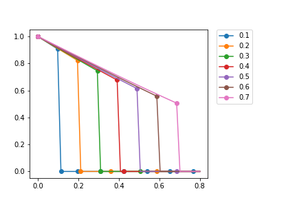
Figure 1: Solution $X/\Delta X$ of the Stokes first problem given by (84) as a function of $y=b/\lambda\sqrt{\mathcal{G}_{\epsilon}}$ at $t/\lambda\in\{.1,.2\dots.7\}$ using numerical integration.

Now, to probe (69) in a more realistic multi-dimensional setting, one may want to first compute simple multi-dimensional solutions possessing symmetries. For instance, using cylindrical coordinates $(R,\Theta)$ and $(r,\theta)$ for both the material and spatial frames, one may want to compute supposedly axisymmetric (also called azimuthal or rotational) $r=R$, $\theta=\Theta+\psi(t,R)$ shear waves [27]:

$$-R|\partial_{t}\psi|^{2} =\partial_{R}S^{rR}+(S^{rR}-S^{\theta\Theta}-\kappa S^{\theta R})/R$$ (85)

$$\partial_{tt}^{2}\psi =R\partial_{R}S^{\theta R}+2S^{\theta R}$$ (86)

with $\kappa(t,R):=R\partial_{R}\psi$, $S^{rR}(t)$ uniform in space, and

$$S^{\theta R}=\kappa-\int_{0}^{t}dse^{\frac{s-t}{\lambda}}\kappa\,,\quad S^{\theta\Theta}=\int_{0}^{t}dse^{\frac{s-t}{\lambda}}\kappa^{2}-\kappa\int_{0}^{t}dse^{\frac{s-t}{\lambda}}\kappa\,.$$

But even if such axisymmetric solutions exist, they do not seem easily constructed anyway. In practice, it is easier to numerically simulate multi-dimensional shear waves with a generic discretization method. This will be the subject of future specialized works. Recall indeed that standard discretization methods need to be adapted, so as to generically simulate SVM on large times with the dissipative inequality as a stability property for the discrete system (indeed, the latter inequality does not correspond to the convex extension of the symmetric-hyperbolic system).

5 Conclusion

In this work, we have derived new symmetric hyperbolic systems of conservation laws to model viscoelastic flows with Upper-Convected Maxwell fluids, either 3D compressible or 2D incompressible with hydrostatic pressure and a free surface. The systems yield the first well-posedness results for causal multi-dimensional viscoelastic motions satisfying the locality principle (i.e. information propagates at finite-speed) as small-time smooth solutions to Cauchy initial-value problems.

The systems also suggest a promising route to unify models for solid and fluid motions. Like K-BKZ theory for viscoelastic fluids with fading memory, they extend standard symmetric-hyperbolic systems (polyconvex elastodynamics and Saint-Venant shallow-water systems). However, they are formulated differently, with the help of an additional material metric variable. Now, using the same methodology, other viscoelastic models with a K-BKZ integro-differential formulation could in fact be similarly formulated as systems of conservation laws. Moreover, varying the relaxation limit of the additional material metric variable should yield (symmetric-hyperbolic formulations of) many possible flow models in between elastic solids and fluids, like elasto-plastic models. New rheological extensions of the polyconvex elastodynamics and Saint-Venant shallow-water systems will be studied in future works.

To precisey apply our new system, in hydraulics in particular, future works shall also consider numerical simulations. Note then that standard discretization methods shall first be adapted like e.g. in [13] to handle large-time motions, since the physical energy functional that dissipates is not the strictly convex functional yielding a strictly convex extension.

References

- [1] S. Benzoni-Gavage and D. Serre. Multi-dimensional hyperbolic partial differential equations. First order systems and applications. Oxford University Press, 2007.
- [2] B. Bernstein, E. A. Kearsley, and L. J. Zapas. A study of stress relaxation with finite strain. Transactions of the Society of Rheology, 7(1):391–410, 1963.
- [3] B. Bernstein, E. A. Kearsley, and L. J. Zapas. Thermodynamics of perfect elastic fluids. Journal of Research of the National Bureau of Standards Section B Mathematics and Mathematical Physics, 68B(3):103, 1964.
- [4] Eugene C. Bingham. Fluidity and plasticity. Mcgraw-Hill Book Company,Inc., 1922.
- [5] R. B. Bird, C. F. Curtiss, R. C. Armstrong, and O. Hassager. Dynamics of Polymeric Liquids, volume 1: Fluid Mechanics. John Wiley & Sons, New York, 1987.
- [6] R. B. Bird, C. F. Curtiss, R. C. Armstrong, and O. Hassager. Dynamics of Polymeric Liquids, volume 2: Kinetic Theory. John Wiley & Sons, New York, 1987.
- [7] Javier Bonet, Antonio J. Gil, and Rogelio Ortigosa. A computational framework for polyconvex large strain elasticity. Comput. Methods Appl. Mech. Engrg., 283:1061–1094, 2015.
- [8] François Bouchut. Entropy satisfying flux vector splittings and kinetic BGK models. Numerische Mathematik, 94:623–672, 2003. 10.1007/s00211-002-0426-9.
- [9] François Bouchut. Nonlinear stability of finite volume methods for hyperbolic conservation laws and well-balanced schemes for sources. Frontiers in Mathematics. Birkhäuser Verlag, Basel, 2004.
- [10] François Bouchut and Sébastien Boyaval. A new model for shallow viscoelastic fluids. M3AS, 23(08):1479–1526, 2013.
- [11] François Bouchut and Sébastien Boyaval. Unified derivation of thin-layer reduced models for shallow free-surface gravity flows of viscous fluids. Eur. J. Mech. B Fluids, 55, Part 1:116–131, 2016.
- [12] Sébastien Boyaval. Derivation and numerical approximation of hyperbolic viscoelastic flow systems: Saint-Venant 2D equations for Maxwell fluids. Technical report, December 2017. working paper or preprint.
- [13] Sébastien Boyaval. Viscoelastic flows with conservation laws. August 2019. working paper or preprint.
- [14] H. S. Carslaw and J. C. Jaeger. Operational Methods in Applied Mathematics. Oxford University Press, New York, 1941.
- [15] Bernard D. Coleman and Walter Noll. The thermodynamics of elastic materials with heat conduction and viscosity. Archive for Rational Mechanics and Analysis, 13(1):167–178, Dec 1963.
- [16] C. M. Dafermos. Hyperbolic conservation laws in continuum physics, volume GM 325. Springer-Verlag, Berlin, 2000.
- [17] A.J.C. de Saint-Venant. Théorie du mouvement non-permanent des eaux, avec application aux crues des rivières et à l’introduction des marées dans leur lit. C. R. Acad. Sc. Paris, 73:147–154, 1871.
- [18] T. W. DeWitt. A rheological equation of state which predicts non–newtonian viscosity, normal stresses, and dynamic moduli. Journal of Applied Physics, 26(7):889–894, 1955.
- [19] M. Doï and S.F. Edwards. The Theory of Polymer Dynamics. Oxford Science, 1998.
- [20] Marco Dressler, Brian J. Edwards, and Hans Christian Öttinger. Macroscopic thermodynamics of flowing polymeric liquids. Rheologica Acta, 38(2):117–136, Jul 1999.
- [21] Brian J. Edwards and Antony N. Beris. Remarks concerning compressible viscoelastic fluid models. Journal of Non-Newtonian Fluid Mechanics, 36:411 – 417, 1990.
- [22] Stefania Ferrari and Fausto Saleri. A new two-dimensional shallow water model including pressure effects and slow varying bottom topography. M2AN Math. Model. Numer. Anal., 38(2):211–234, 2004.
- [23] S. Gavrilyuk, K. Ivanova, and N. Favrie. Multi-dimensional shear shallow water flows: problems and solutions. J. Comput. Phys., 366:252–280, 2018.
- [24] Antoine Gloria, Patrick Le Tallec, and Marina Vidrascu. Foundation, analysis, and numerical investigation of a variational network-based model for rubber. Continuum Mechanics and Thermodynamics, 26(1):1–31, Jan 2014.
- [25] Edwige Godlewski and Pierre-Arnaud Raviart. Numerical approximation of hyperbolic systems of conservation laws, volume 118 of Applied Mathematical Sciences. Springer-Verlag, New York, 1996.
- [26] M. Grmela and P.J. Carreau. Conformation tensor rheological models. Journal of Non-Newtonian Fluid Mechanics, 23:271 – 294, 1987.
- [27] J. B. Haddow and H. A. Erbay. Some aspects of finite amplitude transverse waves in a compressible hyperelastic solid. Quart. J. Mech. Appl. Math., 55(1):17–28, 2002.
- [28] Martien A. Hulsen. A sufficient condition for a positive definite configuration tensor in differential models. J. Non-Newtonian Fluid Mech., 38(1):93–100, 1990.
- [29] Fritz John. Almost global existence of elastic waves of finite amplitude arising from small initial disturbances. Comm. Pure Appl. Math., 41(5):615–666, 1988.
- [30] D.D. Joseph, M. Renardy, and J.C. Saut. Hyperbolicity and change of type in the flow of viscoelastic fluids. Archive for Rational Mechanics and Analysis, 87(3):213–251, 1985.
- [31] DD Joseph and JC Saut. Change of type and loss of evolution in the flow of viscoelastic fluids. Journal of Non-Newtonian Fluid Mechanics, 20:117–141, 1986.
- [32] Tosio Kato. The cauchy problem for quasi-linear symmetric hyperbolic systems. Archive for Rational Mechanics and Analysis, 58(3):181–205, Sep 1975.
- [33] A. Kaye. Non-newtonian flow in incompressible fluids. Technical Report 142, College of Aeronautics Cranfield, 1962. England.
- [34] A. Kaye. Non-newtonian flow in incompressible fluids. Technical Report 142, College of Aeronautics Cranfield, 1962. England.
- [35] V. I. Kondaurov. On conservation laws and symmetrization of equations of the nonlinear theory of thermoelasticity. Dokl. Akad. Nauk SSSR, 256(4):819–823, 1981.
- [36] Jyothi Krishnan and David J. Steigmann. A polyconvex formulation of isotropic elastoplasticity theory. IMA J. Appl. Math., 79(5):722–738, 2014.
- [37] Raz Kupferman, Elihu Olami, and Reuven Segev. Continuum dynamics on manifolds: Application to elasticity of residually-stressed bodies. Journal of Elasticity, 128(1):61–84, Jun 2017.
- [38] R.G. Larson. Constitutive Equations for Polymer Melts and Solutions. Biotechnology Series. Butterworths, 1988.
- [39] Randall J. LeVeque. Finite volume methods for hyperbolic problems. Cambridge Texts in Applied Mathematics. Cambridge University Press, Cambridge, 2002.
- [40] Elliott H. Lieb. Convex trace functions and the Wigner-Yanase-Dyson conjecture. Advances in Math., 11:267–288, 1973.
- [41] Pierre-Louis Lions. Mathematical topics in fluid mechanics. Vol. 1, volume 3 of Oxford Lecture Series in Mathematics and its Applications. The Clarendon Press Oxford University Press, New York, 1996. Incompressible models, Oxford Science Publications.
- [42] A. T. Mackay and T. N. Phillips. On the derivation of macroscopic models for compressible viscoelastic fluids using the generalized bracket framework. J. Non-Newton. Fluid Mech., 266:59–71, 2019.
- [43] A. Majda. Compressible Fluid Flow and Systems of Conservation Laws in Several Space Variables, volume 53 of Applied Mathematical Sciences. Springer-Verlag New York, 1984.
- [44] J.E. Marsden and T.J.R. Hughes. Mathematical Foundations of Elasticity. Dover Civil and Mechanical Engineering. Dover Publications, 2012.
- [45] G.A. Maugin. Continuum Mechanics through the Ages - From the Renaissance to the Twentieth Century: From Hydraulics to Plasticity. Solid Mechanics and Its Applications. Springer International Publishing, 2015.
- [46] James Clerk Maxwell. Iv. on the dynamical theory of gases. Philosophical Transactions of the Royal Society of London, 157:49–88, 1867.
- [47] Alessandro Morando, Yuri Trakhinin, and Paola Trebeschi. Structural stability of shock waves in 2d compressible elastodynamics. Mathematische Annalen, Oct 2019.
- [48] J. G. Oldroyd. On the formulation of rheological equations of state. Proceedings of the Royal Society of London. Series A. Mathematical and Physical Sciences, 200(1063):523–541, 1950.
- [49] Fredrik Olsson. A solver for time-dependent viscoelastic fluid flows. Journal of Non-Newtonian Fluid Mechanics, 51(3):309 – 340, 1994.
- [50] R. G. Owens and T. N. Philips. Computational rheology. Imperial College Press / World Scientific, 2002.
- [51] Ilya Peshkov, Walter Boscheri, Raphaël Loubère, Evgeniy Romenski, and Michael Dumbser. Theoretical and numerical comparison of hyperelastic and hypoelastic formulations for eulerian non-linear elastoplasticity. Journal of Computational Physics, 387:481 – 521, 2019.
- [52] F.R. Phelan, M.F. Malone, and H.H. Winter. A purely hyperbolic model for unsteady viscoelastic flow. Journal of Non-Newtonian Fluid Mechanics, 32(2):197 – 224, 1989.
- [53] S.-D. Poisson. Mémoire sur les équations générales de l’équilibre et du mouvement des corps solides élastiques et des fluides. J. Ec. Polytech., cahier 20(XIII):1–174, 1831.
- [54] M. Renardy. Mathematical Analysis of Viscoelastic Flows, volume 73 of CBMS-NSF Conference Series in Applied Mathematics. SIAM, 2000.
- [55] Michael Renardy. A local existence and uniqueness theorem for a K-BKZ-fluid. Archive for Rational Mechanics and Analysis, 88(1):83–94, 1985.
- [56] C. Speziale. On maxwell models in viscoelasticity that are more computable. International Journal of Non Linear Mechanics, 35:567–571, July 2000.
- [57] Ven te Chow. Open-channel hydraulics. Mc Graw Hill, 1959.
- [58] David H. Wagner. Symmetric-hyperbolic equations of motion for a hyperelastic material. J. Hyperbolic Differ. Equ., 6(3):615–630, 2009.
- [59] D.H. Wagner. Conservation laws, coordinate transformations, and differential forms. In J. Glimm, Graham M.J., Grove J.W., and Plohr B.J., editors, Hyperbolic Problems: Theory, Numerics, Applications, pages 471–477. World Scientific, 1994.
- [60] C. C. Wang and C. Truesdell. Introduction to rational elasticity. Noordhoff International Publishing, Leyden, 1973. Monographs and Textbooks on Mechanics of Solids and Fluids: Mechanics of Continua.
- [61] Wen-An Yong. Newtonian limit of maxwell fluid flows. Arch. Ration. Mech. Anal., 214(3):913–922, 2014.