Random Vector Functional Link Networks for Function Approximation on Manifolds

Abstract

The learning speed of feed-forward neural networks is notoriously slow and has presented a bottleneck in deep learning applications for several decades. For instance, gradient-based learning algorithms, which are used extensively to train neural networks, tend to work slowly when all of the network parameters must be iteratively tuned. To counter this, both researchers and practitioners have tried introducing randomness to reduce the learning requirement. Based on the original construction of Igelnik and Pao, single layer neural-networks with random input-to-hidden layer weights and biases have seen success in practice, but the necessary theoretical justification is lacking. In this paper, we begin to fill this theoretical gap. We then extend this result to the non-asymptotic setting using a concentration inequality for Monte-Carlo integral approximations. We provide a (corrected) rigorous proof that the Igelnik and Pao construction is a universal approximator for continuous functions on compact domains, with approximation error squared decaying asymptotically like $O(1/n)$ for the number $n$ of network nodes. We then extend this result to the non-asymptotic setting, proving that one can achieve any desired approximation error with high probability provided $n$ is sufficiently large. We further adapt this randomized neural network architecture to approximate functions on smooth, compact submanifolds of Euclidean space, providing theoretical guarantees in both the asymptotic and non-asymptotic forms. Finally, we illustrate our results on manifolds with numerical experiments. Machine learning, feed-forward neural networks, function approximation, smooth manifold, Random Vector Functional Link

1 Introduction

In recent years, neural networks have once again triggered an increased interest among researchers in the machine learning community. So-called deep neural networks model functions using a composition of multiple hidden layers, each transforming (possibly non-linearly) the previous layer before building a final output representation (see Krizhevsky et al., 2012; Szegedy et al., 2015; He et al., 2016; Huang et al., 2017; Yang et al., 2018). In machine learning parlance, these layers are determined by sets of weights and biases that can be tuned so that the network mimics the action of a complex function. In particular, a single layer feed-forward neural network (SLFN) with $n$ nodes may be regarded as a parametric function $f_{n}\colon\mathbb{R}^{N}\rightarrow\mathbb{R}$ of the form

$$f_{n}(x)=\sum_{k=1}^{n}v_{k}\rho(\langle w_{k},x\rangle+b_{k}),\quad x\in\mathbb{R}^{N}.$$

Here, the function $\rho\colon\mathbb{R}\rightarrow\mathbb{R}$ is called an activation function and is potentially nonlinear . The parameters of the SLFN are the number of nodes $n\in\mathbb{N}$ in the the hidden layer, the input-to-hidden layer weights and biases $\{w_{k}\}_{k=1}^{n}\subset\mathbb{R}^{N}$ and $\{b_{k}\}_{k=1}^{n}\subset\mathbb{R}$ (resp.), and the hidden-to-output layer weights $\{v_{k}\}_{k=1}^{n}\subset\mathbb{R}$. In this way, neural networks are fundamentally parametric families of functions whose parameters may be chosen to approximate a given function.

It has been shown that any compactly supported continuous function can be approximated with any given precision by a single layer neural network with a suitably chosen number of nodes (Barron, 1993), and harmonic analysis techniques have been used to study stability of such approximations (Candès, 1999). Other recent results that take a different approach directly analyze the capacity of neural networks from a combinatorial point of view (Vershynin, 2020; Baldi and Vershynin, 2019).

While these results ensure existence of a neural network approximating a function, practical applications require construction of such an approximation. The parameters of the neural network can be chosen using optimization techniques to minimize the difference between the network and the function $f\colon\mathbb{R}^{N}\rightarrow\mathbb{R}$ it is intended to model. In practice, the function $f$ is usually not known, and we only have access to a set $\{(x_{k},f(x_{k}))\}_{k=1}^{m}$ of values of the function at finitely many points sampled from its domain, called a training set. The approximation error can be measured by comparing the training data to the corresponding network outputs when evaluated on the same set of points, and the parameters of the neural network $f_{n}$ can be learned by minimizing a given loss function $\mathcal{L}(x_{1},\ldots,x_{k})$; a typical loss function is the sum-of-squares error

$$\mathcal{L}(x_{1},\ldots,x_{k})=\frac{1}{m}\sum_{k=1}^{m}|f(x_{k})-f_{n}(x_{k})|^{2}.$$

The SLFN which approximates $f$ is then determined using an optimization algorithm, such as back-propogation, to find the network parameters which minimize $\mathcal{L}(x_{1},\ldots,x_{k})$. It is known that there exist weights and biases which make the loss function vanish when the number of nodes $n$ is at least $m$, provided the activation function is bounded, nonlinear, and has at least one finite limit at either $\pm\infty$ (Huang and Babri, 1998).

Unfortunately, optimizing the parameters in SLFNs can be difficult. For instance, any non-linearity in the activation function can cause back-propogation to be very time consuming or get caught in local minima of the loss function (Suganthan, 2018). Moreover, deep neural networks can require massive amounts of training data, and so are typically unreliable for applications with very limited data availability, such as agriculture, healthcare, and ecology (Olson et al., 2018).

To address some of the difficulties associated with training deep neural networks, both researchers and practitioners have attempted to incorporate randomness in some way. Indeed, randomization-based neural networks that yield closed form solutions typically require less time to train and avoid some of the pitfalls of traditional neural networks trained using back-propogation (Suganthan, 2018; Schmidt et al., 1992; Te Braake and Van Straten, 1995). One of the popular randomization-based neural network architectures is the Random Vector Functional Link (RVFL) network (Pao and Takefuji, 1992; Igelnik and Pao, 1995), which is a single layer feed-forward neural network in which the input-to-hidden layer weights and biases are selected randomly and independently from a suitable domain and the remaining hidden-to-output layer weights are learned using training data.

By eliminating the need to optimize the input-to-hidden layer weights and biases, RVFL networks turn supervised learning into a purely linear problem. To see this, define ${\rho(X)\in\mathbb{R}^{n\times m}}$ to be the matrix whose $j$th column is $\{\rho(\langle w_{k},x_{j}\rangle+b_{k})\}_{k=1}^{n}$ and $f(X)\in\mathbb{R}^{m}$ the vector whose $j$th entry is $f(x_{j})$. Then the vector $v\in\mathbb{R}^{n}$ of hidden-to-output layer weights is the solution to the matrix-vector equation $f(X)=\rho(X)^{T}v$, which can be solved by computing the Moore-Penrose pseudoinverse of $\rho(X)^{T}$. In fact, there exist weights and biases that make the loss function vanish when the number of nodes $n$ is at least $m$, provided the activation function is smooth (Huang et al., 2006).

Although originally considered in the early- to mid-1990s (Pao and Takefuji, 1992; Pao et al., 1994; Igelnik and Pao, 1995; Pao and Phillips, 1995), RVFL networks have had much more recent success in several modern applications, including time-series data prediction (Chen and Wan, 1999), handwritten word recognition (Park and Pao, 2000), visual tracking (Zhang and Suganthan, 2017a), signal classification (Zhang and Suganthan, 2017b; Katuwal et al., 2018), regression (Vukovic̀ et al., 2018), and forecasting (Tang et al., 2018; Dash et al., 2018). Deep neural network architectures based on RVFL networks have also made their way into more recent literature (Henríquez and Ruz, 2018; Katuwal et al., 2019), although traditional, single layer RVFL networks tend to perform just as well as, and with lower training costs than, their multi-layer counterparts (Katuwal et al., 2019).

Even though RVFL networks are proving their usefulness in practice, the supporting theoretical framework is currently lacking (see Zhang et al., 2019). Most theoretical research into the approximation capabilities of deep neural networks centers around two main concepts: universal approximation of functions on compact domains and point-wise approximation on finite training sets (Huang et al., 2006). For instance, in the early 1990s it was shown that multi-layer feed-forward neural networks having activation functions that are continuous, bounded, and non-constant are universal approximators (in the $L^{p}$ sense for $1\leq p<\infty$) of continuous functions on compact domains (Hornik, 1991; Leshno et al., 1993). The most notable result in the existing literature regarding the universal approximation capability of RVFL networks is due to B. Igelnik and Y.H. Pao in the mid-1990s, who showed that such neural networks can universally approximate continuous functions on compact sets (Igelnik and Pao, 1995); the noticeable lack of results since has left a sizable gap between theory and practice. In this paper, we begin to bridge this gap by further improving the Igelnik and Pao result, and bringing the mathematical theory behind RFVL networks into the modern spotlight. Below, we introduce the notation that will be used throughout this paper, and describe our main contributions.

1.1 Notation

For a function $f\colon\mathbb{R}^{N}\rightarrow\mathbb{R}$, the set $\mathrm{supp}(f)\subset\mathbb{R}^{N}$ denotes the support of $f$. We denote by $C_{c}(\mathbb{R}^{N})$ and $C_{0}(\mathbb{R}^{N})$ the classes of continuous functions mapping $\mathbb{R}^{N}$ to $\mathbb{R}$ whose support sets are compact and vanish at infinity, respectively. Given a set $S\subset\mathbb{R}^{N}$, we define its radius to be $\mathrm{rad}(S):=\sup_{x\in S}\|x\|_{2}$; moreover, if $\mathrm{d}\mu$ denotes the uniform volume measure on $S$, then we write $\mathrm{vol}(S):=\int_{S}\mathrm{d}\mu$ to represent the volume of $S$. For any probability distribution $P\colon\mathbb{R}^{N}\rightarrow[0,1]$, a random variable $X$ distributed according to $P$ is denoted by $X\sim P$, and we write its expectation as $\mathbb{E}X:=\int_{\mathbb{R}^{N}}X\mathrm{d}P$. The open $\ell_{p}$ ball of radius $r>0$ centered at $x\in\mathbb{R}^{N}$ is denoted by $B_{p}^{N}(x,r)$ for all $1\leq p\leq\infty$; the $\ell_{p}$ unit-ball centered at the origin is abbreviated $B_{p}^{N}$. Given a fixed $\delta>0$ and a set $S\subset\mathbb{R}^{N}$, a minimal $\delta$-net for $S$, which we denote $\mathcal{C}(\delta,S)$, is the smallest subset of $S$ satisfying $S\subset\cup_{x\in\mathcal{C}(\delta,S)}B_{2}^{N}(x,\delta)$; the $\delta$-covering number of $S$ is the cardinality of a minimal $\delta$-net for $S$ and is denoted $\mathcal{N}(\delta,S):=|\mathcal{C}(\delta,S)|$.

1.2 Main results

In this paper, we study the uniform approximation capabilities of RVFL networks. More specifically, we consider the problem of using RVFL networks to estimate a continuous, compactly supported function on $N$-dimensional Euclidean space.

The first theoretical result on approximating properties of RVFL networks, due to Igelnik and Pao, guarantees that continuous functions may be universally approximated on compact sets using RVFL networks, provided the number of nodes $n\in\mathbb{N}$ in the network is allowed to go to infinity (Igelnik and Pao, 1995). Moreover, it shows that the mean square error of the approximation vanishes at a rate proportional to $1/n$. At the time, this result was state-of-the-art and justified how RVFL networks were used in practice. However, the original theorem, although correct in spirit, is not technically correct. In fact, several aspects of the proof technique are flawed. Some of the minor flaws are mentioned in Li et al. (1997), but the subsequent revisions do not address the more major issues that we tackle here — see Remark 1.2. Thus, our first contribution to the theory of RVFL networks is a corrected version of the original Igelnik and Pao theorem:

Theorem 1.1 (Igelnik and Pao (1995)).

Let $f\in C_{c}(\mathbb{R}^{N})$ with $K:=\mathrm{supp}(f)$ and fix any activation function $\rho$, such that either $\rho\in L^{1}(\mathbb{R})\cap L^{\infty}(\mathbb{R})$ or $\rho$ is differentiable with $\rho^{\prime}\in L^{1}(\mathbb{R})\cap L^{\infty}(\mathbb{R}).$ For any $\varepsilon>0$, there exist distributions from which input weights $\{w_{k}\}_{k=1}^{n}$ and biases $\{b_{k}\}_{k=1}^{n}$ are drawn, and there exist hidden-to-output layer weights $\{v_{k}\}_{k=1}^{n}\subset\mathbb{R}$ that depend on the realization of weights and biases, such that the sequence of RVFL networks $\{f_{n}\}_{n=1}^{\infty}$ defined by

$$f_{n}(x):=\sum_{k=1}^{n}v_{k}\rho(\langle w_{k},x\rangle+b_{k})\quad\text{ for $x\in K$}$$

satisfies

$$\mathbb{E}\int_{K}|f(x)-f_{n}(x)|^{2}\mathrm{d}x<\varepsilon+O(1/n),$$

as $n\to\infty.$

For a more precise formulation of Theorem 1.1 and its proof, we refer the reader to Theorem 3.1 and Section 3.

Remark 1.2.

1. Even though in Theorem 1.1 we only claim existence of the distribution for input weights $\{w_{k}\}_{k=1}^{n}$ and biases $\{b_{k}\}_{k=1}^{n}$, such a distribution is actually constructed in the proof. Namely, for any $\varepsilon>0$, there exist constants $\alpha,\Omega>0$ such that the random variables

   $$w_{k} \sim\mathrm{Unif}([-\alpha\Omega,\alpha\Omega]^{N});$$

   $$y_{k} \sim\mathrm{Unif}(K);$$

   $$u_{k} \sim\mathrm{Unif}([-\tfrac{\pi}{2}(2L+1),\tfrac{\pi}{2}(2L+1)]),\quad\text{where $L:=\lceil\tfrac{2N}{\pi}\mathrm{rad}(K)\Omega-\tfrac{1}{2}\rceil$},$$

   are independently drawn from their associated distributions, and $b_{k}:=-\langle w_{k},y_{k}\rangle-\alpha u_{k}$.

2. We note that, unlike the original theorem statement in Igelnik and Pao (1995), Theorem 1.1 does not show exact convergence of the sequence of constructed RVFL networks $f_{n}$ to the original function $f$. Indeed, it only ensures that the limit $f_{n}$ is $\varepsilon$-close to $f$. This should still be sufficient for practical applications since, given a desired accuracy level $\varepsilon>0$, one can find values of $\alpha,\Omega,n$ such that this accuracy level is achieved on average. Exact convergence can be proved if one replaces $\alpha$ and $\Omega$ in the distribution described above by sequences $\{\alpha_{n}\}_{n=1}^{\infty}$ and $\{\Omega_{n}\}_{n=1}^{\infty}$ of positive numbers, both tending to infinity with $n$. In this setting, however, there is no guaranteed rate of convergence; moreover, as $n$ increases, the ranges of the random variables $\{w_{k}\}_{k=1}^{n}$ and $\{u_{k}\}_{k=1}^{n}$ become increasingly larger, which may cause problems in practical applications.

3. The approach we take to construct the RVFL network approximating a function $f$ allows one to compute the output weights $\{v_{k}\}_{k=1}^{n}$ exactly (once the realization of random parameters is fixed), in the case where the function $f$ is known. For the details, we refer the reader to equations (6) and (8) in the proof of Theorem 1.1. If we only have access to a training set that is sufficiently large and uniformly distributed over the support of $f$, these formulas can be used to compute the output weights approximately, instead of solving the least squares problem.

One of the drawbacks of Theorem 1.1 is that the mean square error guarantee is asymptotic in the number of nodes used in the neural network. This is clearly impractical for applications, and so it is desirable to have a more explicit error bound for each fixed number $n$ of nodes used. To this end, we provide a new, non-asymptotic version of Theorem 1.1, which provides an error guarantee with high probability whenever the number of network nodes is large enough, albeit at the price of an additional Lipschitz requirement on the activation function:

Theorem 1.3.

Let $f\in C_{c}(\mathbb{R}^{N})$ with $K:=\mathrm{supp}(f)$ and fix any activation function ${\rho\in L^{1}(\mathbb{R})\cap L^{\infty}(\mathbb{R})}$. Suppose further that $\rho$ is $\kappa$-Lipschitz on $\mathbb{R}$ for some $\kappa>0$. For any $\varepsilon>0$ and $\eta\in(0,1)$, suppose that $n\geq C(N,f,\rho)\varepsilon^{-1}\log(\eta^{-1}/\varepsilon),$ where $C(N,f,\rho)$ is independent of $\varepsilon$ and $\eta$ and depends on $f$, $\rho$, and superexponentially on $N$. Then there exist distributions from which input weights $\{w_{k}\}_{k=1}^{n}$ and biases $\{b_{k}\}_{k=1}^{n}$ are drawn, and there exist hidden-to-output layer weights $\{v_{k}\}_{k=1}^{n}\subset\mathbb{R}$ that depend on the realization of weights and biases, such that the RVFL network defined by

$$f_{n}(x):=\sum_{k=1}^{n}v_{k}\rho(\langle w_{k},x\rangle+b_{k})\quad\text{ for $x\in K$}$$

satisfies

$$\int_{K}|f(x)-f_{n}(x)|^{2}\mathrm{d}x<\varepsilon$$

with probability at least $1-\eta$.

For simplicity, the bound on the number $n$ of the nodes on the hidden layer here is rough. For a more precise formulation of this result that contains a bound with explicit constant, we refer the reader to Theorem 4.1 in Section 4. We also note that the distribution of the input weight and bias here can be selected as described in Remark 1.2.

The constructions of RVFL networks presented in Theorems 1.1 and 1.3 depend heavily on the dimension of the ambient space $\mathbb{R}^{N}$. If $N$ is small, this dependence does not present much of a problem. However, many modern applications require the ambient dimension to be large. Fortunately, a common assumption in practice is that support of the signals of interest lie on a lower-dimensional manifold embedded in $\mathbb{R}^{N}$. In this paper, we propose a new RVFL network architecture for approximating continuous functions defined on smooth compact manifolds that allows to replace the dependence on the ambient dimension $N$ with dependence on the manifold intrinsic dimension. We show that RVFL approximation results can be extended to this setting. More precisely, we prove the following analog of Theorem 1.3.

Theorem 1.4.

Let $\mathcal{M}\subset\mathbb{R}^{N}$ be a smooth, compact $d$-dimensional manifold with finite atlas $\{(U_{j},\phi_{j})\}_{j\in J}$ and $f\in C(\mathcal{M})$. Fix any activation function $\rho\in L^{1}(\mathbb{R})\cap L^{\infty}(\mathbb{R})$ such that $\rho$ is $\kappa$-Lipschitz on $\mathbb{R}$ for some $\kappa>0$. For any $\varepsilon>0$ and $\eta\in(0,1)$, suppose $n\geq C(d,f,\rho)\varepsilon^{-1}\log(\eta^{-1}/\varepsilon),$ where $C(d,f,\rho)$ is independent of $\varepsilon$ and $\eta$ and depends on $f$, $\rho$, and superexponentially on $d$. Then there exists an RVFL-like approximation $f_{n}$ of the function $f$ with a parameter selection similar to the Theorem 1.1 construction that satisfies

$$\int_{\mathcal{M}}|f(x)-f_{n}(x)|^{2}\mathrm{d}x<\varepsilon$$

with probability at least $1-\eta$.

For a the construction of the RVFL-like approximation $f_{n}$ and a more precise formulation of this result and a manifold analog of Theorem 1.1, we refer the reader to Section 5.1 and Theorems 5.1 and 5.4. We note that the approximation $f_{n}$ here is not obtained as a single RVFL network construction, but rather as a combination of several RVFL networks in local manifold coordinates.

1.3 Organization

The remaining part of the paper is organized as follows. In Section 2, we discuss some theoretical preliminaries on concentration bounds for Monte-Carlo integration and on smooth compact manifolds. Monte-Carlo integration is an essential ingredient in our construction of RVFL networks approximating a given function, and we use the results listed in this section to establish approximation error bounds. Theorem 1.1 is proven in Section 3, where we break down the proof into four main steps, constructing a limit-integral representation of the function to be approximated in Lemmas 3.3 and 3.4, then using Monte-Carlo approximation of the obtained integral to construct an RVFL network in Lemma 3.5, and, finally, establishing approximation guarantees for the constructed RVFL network. The proofs of Lemmas 3.3, 3.4, and 3.5 can be found in Sections A.1, A.2,  and A.3, respectively. We further study properties of the constructed RVFL networks and prove the non-asymptotic approximation result of Theorem 1.3 in Section 4. In Section 5, we generalize our results and propose a new RVFL network architecture for approximating continuous functions defined on smooth compact manifolds. We show that RVFL approximation results can be extended to this setting by proving an analog of Theorem 1.1 in Section 5.2 and Theorem 1.4 in Section A.5. Finally, in Section 6, we provide numerical evidence to illustrate the result of Theorem 1.4.

2 Theoretical Preliminaries

In this section, we briefly introduce supporting material and theoretical results which we will need in later sections. This material is far from exhaustive, and is meant to be a survey of definitions, concepts, and key results.

2.1 A concentration bound for classic Monte-Carlo integration

A crucial piece of the proof technique employed in Igelnik and Pao (1995), which we will use repeatedly, is the use of the Monte-Carlo method to approximate high-dimensional integrals. As such, we start with the background on Monte-Carlo integration. The following introduction is adapted from the material in Dick et al. (2013).

Let $f\colon\mathbb{R}^{N}\rightarrow\mathbb{R}$ and $S\subset\mathbb{R}^{N}$ a compact set. Suppose we want to estimate the integral ${I(f,S):=\int_{S}f\mathrm{d}\mu}$, where $\mu$ is the uniform measure on $S$. The classic Monte Carlo method does this by an equal-weight cubature rule,

$$I_{n}(f,S):=\frac{\mathrm{vol}(S)}{n}\sum_{j=1}^{n}f(x_{j}),$$

where $\{x_{j}\}_{j=1}^{n}$ are independent identically distributed uniform random samples from $S$ and ${\mathrm{vol}(S):=\int_{S}d\mu}$ is the volume of $S$. In particular, note that $\mathbb{E}I_{n}(f,S)=I(f,S)$ and

$$\mathbb{E}I_{n}(f,S)^{2}=\frac{1}{n}\big{(}\mathrm{vol}(S)I(f^{2},S)+(n-1)I(f,S)^{2}\big{)}.$$

Let us define the quantity

$$\sigma(f,S)^{2}:=\frac{I(f^{2},S)}{\mathrm{vol}(S)}-\frac{I(f,S)^{2}}{\mathrm{vol}^{2}(S)}.$$ (1)

It follows that the random variable $I_{n}(f)$ has mean $I(f,S)$ and variance $\mathrm{vol}^{2}(S)\sigma(f,S)^{2}/n$. Hence, by the Central Limit Theorem, provided that $0<\mathrm{vol}^{2}(S)\sigma(f,S)^{2}<\infty$, we have

$$\lim_{n\rightarrow\infty}\mathbb{P}\Big{(}|I_{n}(f,S)-I(f,S)|\leq\frac{C\varepsilon(f)}{\sqrt{n}}\Big{)}=(2\pi)^{-1/2}\int_{-C}^{C}e^{-x^{2}/2}\mathrm{d}x$$

for any constant $C>0$, where $\varepsilon(f,S):={\mathrm{vol}(S)\sigma(f,S)}$. This yields the following well-known result:

Theorem 2.1.

For any $f\in L^{2}(S,\mu)$, the mean-square error of the Monte Carlo approximation $I_{n}(f,S)$ satisfies

$$\mathbb{E}\big{|}I_{n}(f,S)-I(f,S)\big{|}^{2}=\frac{\mathrm{vol}^{2}(S)\sigma(f,S)^{2}}{n},$$

where the expectation is taken with respect to the random variables $\{x_{j}\}_{j=1}^{n}$ and $\sigma(f,S)$ is defined in (1).

In particular, Theorem 2.1 implies $\mathbb{E}\big{|}I_{n}(f,S)-I(f,S)\big{|}^{2}=O(1/n),$ as $n\to\infty.$

In the non-asymptotic setting, we are interested in obtaining a useful bound on the probability ${\mathbb{P}(|I_{n}(f,S)-I(f,S)|\geq t)}$ for all $t>0$. The following lemma follows from a generalization of Bennett’s inequality (Theorem 7.6 in Ledoux (2001); see also Massart (1998); Talagrand (1996)).

Lemma 2.2.

For any $f\in L^{2}(S)$ and $n\in\mathbb{N}$ we have

$$\mathbb{P}\Big{(}|I_{n}(f,S)-I(f,S)|\geq t\Big{)}\leq 3\exp\left(-\frac{nt}{CK}\log\left(1+\frac{Kt}{\displaystyle\mathrm{vol}(S)I(f^{2},S)}\right)\right)$$

for all $t>0$ and a universal constant $C>0$, provided $\lvert\mathrm{vol}(S)f(x)\rvert\leq K$ for almost every $x\in S$.

2.2 Smooth, compact manifolds in Euclidean space

In this section we review several concepts of smooth manifolds that will be useful to us later. Many of the definitions and results that follow can be found, for instance, in Shaham et al. (2018). Let $\mathcal{M}\subset\mathbb{R}^{N}$ be a smooth, compact $d$-dimensional manifold. A chart for $\mathcal{M}$ is a pair $(U,\phi)$ such that $U\subset\mathcal{M}$ is an open set and $\phi\colon U\rightarrow\mathbb{R}^{d}$ is a homeomorphism. One way to interpret a chart is as a tangent space at some point $x\in U$; in this way, a chart defines a Euclidean coordinate system on $U$ via the map $\phi$. A collection $\{(U_{j},\phi_{j})\}_{j\in J}$ of charts defines an atlas for $\mathcal{M}$ if $\cup_{j\in J}U_{j}=\mathcal{M}$. We now define a special collection of functions on $\mathcal{M}$ called a partition of unity.

Definition 2.3.

Let $\mathcal{M}\subset\mathbb{R}^{N}$ be a smooth manifold. A partition of unity of $\mathcal{M}$ with respect to an open cover $\{U_{j}\}_{j\in J}$ of $\mathcal{M}$ is a family of nonnegative smooth functions $\{\eta_{j}\}_{j\in J}$ such that for every $x\in\mathcal{M}$ we have $1=\sum_{j\in J}\eta_{j}(x)$ and, for every $j\in J$, $\mathrm{supp}(\eta_{j})\subset U_{j}$.

It is known that if $\mathcal{M}$ is compact there exists a partition of unity of $\mathcal{M}$ such that $\mathrm{supp}(\eta_{j})$ is compact for all $j\in J$ (see Tu, 2010). In particular, such a partition of unity exists for any open cover of $\mathcal{M}$ corresponding to an atlas.

Fix an atlas $\{(U_{j},\phi_{j})\}_{j\in J}$ for $\mathcal{M}$, as well as the corresponding, compactly supported partition of unity $\{\eta_{j}\}_{j\in J}$. Then we have the following, useful result (see Shaham et al., 2018, Lemma 4.8).

Lemma 2.4.

Let $\mathcal{M}\subset\mathbb{R}^{N}$ be a smooth, compact manifold with atlas $\{(U_{j},\phi_{j})\}_{j\in J}$ and compactly supported partition of unity $\{\eta_{j}\}_{j\in J}$. For any $f\in C(\mathcal{M})$ we have

$$f(x)=\sum_{\{j\in J\colon x\in U_{j}\}}(\hat{f}_{j}\circ\phi_{j})(x)$$

for all $x\in\mathcal{M}$, where

$$\hat{f}_{j}(z):=\begin{cases}f(\phi_{j}^{-1}(z))\,\eta_{j}(\phi_{j}^{-1}(z))\quad&z\in\phi_{j}(U_{j})\\ 0&\text{otherwise}.\end{cases}$$

In later sections, we use the representation of Lemma 2.4 to integrate functions $f\in C(\mathcal{M})$ over $\mathcal{M}$. To this end, for each $j\in J$, let $D\phi_{j}(y)$ denote the differential of $\phi_{j}$ at $y\in U_{j}$, which is a map from the tangent space $T_{y}\mathcal{M}$ into $\mathbb{R}^{d}$. One may interpret $D\phi_{j}(y)$ as the matrix representation of a basis for the cotangent space at $y\in U_{j}$. As a result, $D\phi_{j}(y)$ is necessarily invertible for each $y\in U_{j}$, and so we know that $|\det(D\phi_{j}(y))|>0$ for each $y\in U_{j}$. Hence, it follows by the change of variables theorem that

$$\int_{\mathcal{M}}f(x)\mathrm{d}x=\int_{\mathcal{M}}\sum_{\{j\in J\colon x\in U_{j}\}}(\hat{f}_{j}\circ\phi_{j})(x)\mathrm{d}x=\sum_{j\in J}\int_{\phi_{j}(U_{j})}\frac{\hat{f}_{j}(z)}{|\det(D\phi_{j}(\phi_{j}^{-1}(z)))|}\mathrm{d}z.$$ (2)

3 Proof of Theorem 1.1

We split the proof of the theorem into two parts, the first handling the case $\rho\in L^{1}(\mathbb{R})\cap L^{\infty}(\mathbb{R})$ and the second, addressing the case $\rho^{\prime}\in L^{1}(\mathbb{R})\cap L^{\infty}(\mathbb{R}).$

3.1 Proof of Theorem 1.1 when $\rho\in L^{1}(\mathbb{R})\cap L^{\infty}(\mathbb{R})$

We begin by restating the theorem in a form that explicitly includes the distributions that we draw our random variables from.

Theorem 3.1 (Igelnik and Pao (1995)).

Let $f\in C_{c}(\mathbb{R}^{N})$ with $K:=\mathrm{supp}(f)$ and fix any activation function $\rho\in L^{1}(\mathbb{R})\cap L^{\infty}(\mathbb{R}).$ For any $\varepsilon>0$, there exist constants $\alpha,\Omega>0$ such that the following holds: If, for $k\in\mathbb{N}$, the random variables

$$w_{k} \sim\mathrm{Unif}([-\alpha\Omega,\alpha\Omega]^{N});$$

$$y_{k} \sim\mathrm{Unif}(K);$$

$$u_{k} \sim\mathrm{Unif}([-\tfrac{\pi}{2}(2L+1),\tfrac{\pi}{2}(2L+1)]),\quad\text{where $L:=\lceil\tfrac{2N}{\pi}\mathrm{rad}(K)\Omega-\tfrac{1}{2}\rceil$},$$

are independently drawn from their associated distributions, and

$$b_{k}:=-\langle w_{k},y_{k}\rangle-\alpha u_{k},$$

then there exist hidden-to-output layer weights $\{v_{k}\}_{k=1}^{n}\subset\mathbb{R}$ (that depend on the realization of the weights $\{w_{k}\}_{k=1}^{n}$ and biases $\{b_{k}\}_{k=1}^{n}$) such that the sequence of RVFL networks $\{f_{n}\}_{n=1}^{\infty}$ defined by

$$f_{n}(x):=\sum_{k=1}^{n}v_{k}\rho(\langle w_{k},x\rangle+b_{k})\quad\text{ for $x\in K$}$$

satisfies

$$\mathbb{E}\int_{K}|f(x)-f_{n}(x)|^{2}\mathrm{d}x\leq\varepsilon+O(1/n)$$

as $n\to\infty.$

Proof 3.2.

Our proof technique is based on that introduced by Igelnik and Pao, and can be divided into four steps. The first three steps essentially consist of Lemma 3.3, Lemma 3.4, and Lemma 3.5, and the final step combines them to obtain the desired result. First, the function $f$ is approximated by a convolution, given in Lemma 3.3. The proof of this result can be found in Section A.1.

Lemma 3.3.

Let $f\in C_{0}(\mathbb{R}^{N})$ and $h\in L^{1}(\mathbb{R}^{N})$ with $\int_{\mathbb{R}^{N}}h(z)\mathrm{d}z=1.$ Define, for $\Omega>0,$

$$h_{\Omega}(y):=\Omega^{N}h(\Omega y).$$ (3)

Then we have

$$f(x)=\lim_{\Omega\to\infty}(f*h_{\Omega})(x)$$ (4)

uniformly for all $x\in\mathbb{R}^{N}$.

Next, we represent $f$ as the limiting value of a multidimensional integral over the parameter space. In particular, we replace $(f*h_{\Omega})(x)$ in the convolution identity (4) with a function of the form $\int_{K}F(y)\rho(\langle w,x\rangle+b(y))\mathrm{d}y$, as this will introduce the RVFL structure we require. To achieve this, we first use a truncated cosine function in place of the activation function $\rho$ and then switch back to a general activation function.

To that end, for each fixed $\Omega>0$, let $L=L(\Omega):=\lceil\frac{2N}{\pi}\mathrm{rad}(K)\Omega-\frac{1}{2}\rceil$ and define $\cos_{\Omega}\colon\mathbb{R}\rightarrow[-1,1]$ by

$$\cos_{\Omega}(x):=\begin{cases}\cos(x)\qquad&x\in[-\tfrac{1}{2}(2L+1)\pi,\tfrac{1}{2}(2L+1)\pi],\\ 0&\text{otherwise}.\end{cases}$$ (5)

Moreover, introduce the functions

$$\begin{split}F_{\alpha,\Omega}(y,w,u)&:=\frac{\alpha}{(2\pi)^{N}}f(y)\cos_{\Omega}(u)\prod_{j=1}^{N}\phi(w(j)/\Omega),\\ b_{\alpha}(y,w,u)&:=-\alpha(\langle w,y\rangle+u)\end{split}$$ (6)

where $y,w\in\mathbb{R}^{N}$ and $u\in\mathbb{R}$ and $\phi=A*A$ for any even function $A\in C^{\infty}(\mathbb{R})$ supported on $[-\tfrac{1}{2},\tfrac{1}{2}]$ s.t. $\lVert A\rVert_{2}=1.$ Then we have the following lemma, a detailed proof of which can be found in Section A.2.

Lemma 3.4.

Let $f\in C_{c}(\mathbb{R}^{N})$ and $\rho\in L^{1}(\mathbb{R})$ with $K:=\mathrm{supp}(f)$ and $\int_{\mathbb{R}}\rho(z)\mathrm{d}z=1$. Define $F_{\alpha,\Omega}$ and $b_{\alpha}$ as in (6) for all $\alpha>0.$ Then, for $L:=\lceil\frac{2N}{\pi}\mathrm{rad}(K)\Omega-\frac{1}{2}\rceil$, we have

$$f(x)=\lim_{\Omega\rightarrow\infty}\lim_{\alpha\rightarrow\infty}\int_{K(\Omega)}F_{\alpha,\Omega}(y,w,u)\rho\big{(}\alpha\langle w,x\rangle+b_{\alpha}(y,w,u)\big{)}\mathrm{d}y\mathrm{d}w\mathrm{d}u$$ (7)

uniformly for every $x\in K$, where $K(\Omega):=K\times[-\Omega,\Omega]^{N}\times[-\frac{\pi}{2}(2L+1),\frac{\pi}{2}(2L+1)]$.

The next step in the proof of Theorem 3.1 is to approximate the integral in (7) using the Monte-Carlo method. Define $v_{k}:=\frac{\mathrm{vol}(K(\Omega))}{n}F_{\alpha,\Omega}\Big{(}y_{k},\frac{w_{k}}{\alpha},u_{k}\Big{)}$ for $k=1,\ldots,n$, and the random variables $\{f_{n}\}_{n=1}^{\infty}$ by

$$f_{n}(x):=\sum_{k=1}^{n}v_{k}\rho\big{(}\langle w_{k},x\rangle+b_{k}\big{)}.$$ (8)

Then, we have the following lemma that is proven in Section A.3.

Lemma 3.5.

Let $f\in C_{c}(\mathbb{R}^{N})$ and $\rho\in L^{1}(\mathbb{R})\cap L^{\infty}(\mathbb{R})$ with $K:=\mathrm{supp}(f)$ and $\int_{\mathbb{R}}\rho(z)\mathrm{d}z=1$. Then, as $n\to\infty$, we have

$$\mathbb{E}\int_{K}\left|\int_{K(\Omega)}F_{\alpha,\Omega}(y,w,u)\rho\big{(}\alpha\langle w,x\rangle+b_{\alpha}(y,w,u)\big{)}\mathrm{d}y\mathrm{d}w\mathrm{d}u-f_{n}(x)\right|^{2}\mathrm{d}x=O(1/n),$$ (9)

where $K(\Omega):=K\times[-\Omega,\Omega]^{N}\times[-\frac{\pi}{2}(2L+1),\frac{\pi}{2}(2L+1)]$ and $L:=\lceil\frac{2N}{\pi}\mathrm{rad}(K)\Omega-\frac{1}{2}\rceil$.

To complete the proof of Theorem 3.1 we combine the limit representation (7) with the Monte-Carlo error guarantee (9) and show that, given any $\varepsilon>0$, there exist $\alpha,\Omega>0$ such that

$$\mathbb{E}\int_{K}|f(x)-f_{n}(x)|^{2}\mathrm{d}x\leq\varepsilon+O(1/n)$$

as $n\to\infty.$ To this end, let $\varepsilon^{\prime}>0$ be arbitrary and consider the integral $I(x;p)$ given by

$$I(x;p):=\int_{K(\Omega)}\Big{(}F_{\alpha,\Omega}(y,w,u)\rho\big{(}\alpha\langle w,x\rangle+b_{\alpha}(y,w,u)\big{)}\Big{)}^{p}\mathrm{d}y\mathrm{d}w\mathrm{d}u$$ (10)

for $x\in K$ and $p\in\mathbb{N}$. By (7), there exist $\alpha,\Omega>0$ such that $|f(x)-I(x;1)|<\varepsilon^{\prime}$ holds for every $x\in K$, and so it follows that

$$\big{|}f(x)-f_{n}(x)\big{|}<\varepsilon^{\prime}+\big{|}I(x;1)-f_{n}(x)\big{|}$$

for every $x\in K$. Jensen’s inequality now yields that

$$\mathbb{E}\int_{K}|f(x)-f_{n}(x)|^{2}\mathrm{d}x\leq 2\mathrm{vol}(K)(\varepsilon^{\prime})^{2}+2\mathbb{E}\int_{K}\big{|}I(x;1)-f_{n}(x)\big{|}^{2}\mathrm{d}x$$ (11)

By (9), we know that the second term on the right-hand side of (11) is $O(1/n).$ Therefore, we have

$$\mathbb{E}\int_{K}|f(x)-f_{n}(x)|^{2}\mathrm{d}x\leq 2\mathrm{vol}(K)(\varepsilon^{\prime})^{2}+O(1/n)$$

and so the proof is completed by taking $\varepsilon^{\prime}=\sqrt{\varepsilon/2\mathrm{vol}(K)}$ and choosing $\alpha,\Omega>0$ accordingly.

3.2 Proof of Theorem 1.1 when $\rho^{\prime}\in L^{1}(\mathbb{R})\cap L^{2}(\mathbb{R})$

The full statement of the theorem is identical to that of Theorem 3.1 albeit now with ${\rho^{\prime}\in L^{1}(\mathbb{R})\cap L^{2}(\mathbb{R})}$, so we omit it for brevity. Its proof is also similar to the proof of the case where $\rho\in L^{1}(\mathbb{R})\cap L^{2}(\mathbb{R})$ with some key modifications. Namely, one uses an integration by parts argument to modify the part of the proof corresponding to Lemma 3.4. The details of this argument are presented in the appendix, Section A.4.

4 Proof of Theorem 1.3

In this section we prove the non-asymptotic result for RVFL networks in $\mathbb{R}^{N}$, and we begin with a more precise statement of the theorem that makes all the dimensional dependencies explicit.

Theorem 4.1.

Consider the hypotheses of Theorem 3.1 and suppose further that $\rho$ is $\kappa$-Lipschitz on $\mathbb{R}$ for some $\kappa>0$. For any

$$0<\delta<\frac{\sqrt{\varepsilon}}{8\sqrt{2N}\kappa\alpha^{2}M\Omega(\Omega/\pi)^{N}\mathrm{vol}^{3/2}(K)(\pi+2N\mathrm{rad}(K)\Omega)},$$

Suppose

$$n \geq\frac{c\Sigma\alpha(\Omega/\pi)^{N}(\pi+2N\mathrm{rad}(K)\Omega)\log(3\eta^{-1}\mathcal{N}(\delta,K))}{\sqrt{\varepsilon}\log\big{(}1+\frac{\sqrt{\varepsilon}}{\Sigma\alpha(\Omega/\pi)^{N}(\pi+2N\mathrm{rad}(K)\Omega)}\big{)}},$$

where $M:=\sup_{x\in K}|f(x)|$, $c>0$ is a numerical constant, and $\Sigma$ is a constant depending on $f$ and $\rho$, and let parameters $\{w_{k}\}_{k=1}^{n}$, $\{b_{k}\}_{k=1}^{n}$, and $\{v_{k}\}_{k=1}^{n}$ be as in Theorem 3.1. Then the RVFL network defined by

$$f_{n}(x):=\sum_{k=1}^{n}v_{k}\rho(\langle w_{k},x\rangle+b_{k})\quad\text{ for $x\in K$}$$

satisfies

$$\int_{K}|f(x)-f_{n}(x)|^{2}\mathrm{d}x<\varepsilon$$

with probability at least $1-\eta$.

Proof 4.2.

Let $f\in C_{c}(\mathbb{R}^{N})$ with $K:=\mathrm{supp}(f)$ and suppose $\varepsilon>0$, $\eta\in(0,1)$ are fixed. Take an arbitrarily $\kappa$-Lipschitz activation function $\rho\in L^{1}(\mathbb{R})\cap L^{\infty}(\mathbb{R}).$ We wish to show that there exists an RVFL network $\{f_{n}\}_{n=1}^{\infty}$ defined on $K$ that satisfies the error bound

$$\int_{K}|f(x)-f_{n}(x)|^{2}\mathrm{d}x<\varepsilon$$

with probability at least $1-\eta$ when $n$ is chosen sufficiently large. The proof is obtained by modifying the proof of Theorem 3.1 for the asymptotic case.

We begin by repeating the first two steps in the proof of Theorem 3.1 from Sections A.1 and A.2. In particular, by Lemma 3.4 we have the representation (7), namely,

$$f(x)=\lim_{\Omega\rightarrow\infty}\lim_{\alpha\rightarrow\infty}\int_{K(\Omega)}F_{\alpha,\Omega}(y,w,u)\rho\big{(}\alpha\langle w,x\rangle+b_{\alpha}(y,w,u)\big{)}\mathrm{d}y\mathrm{d}w\mathrm{d}u$$

holds uniformly for all $x\in K$. Hence, if we define the random variables $f_{n}$ and $I_{n}$ from Section A.3 as in (8) and (29), respectively, we seek a uniform bound on the quantity

$$|f(x)-f_{n}(x)|\leq|f(x)-I(x;1)|+|I_{n}(x)-I(x;1)|$$

over the compact set $K$, where $I(x;1)$ is given by (10) for all $x\in K$. Since equation (7) allows us to fix $\alpha,\Omega>0$ such that

$$|f(x)-I(x;1)|=\Big{|}f(x)-\int_{K(\Omega)}F_{\alpha,\Omega}(y,w,u)\rho\big{(}\alpha\langle w,x\rangle+b_{\alpha}(y,w,u)\big{)}\mathrm{d}y\mathrm{d}w\mathrm{d}u\Big{|}<\sqrt{\frac{\varepsilon}{2\mathrm{vol}(K)}}$$

holds for every $x\in K$ simultaneously, the result follows if we show that, with high probability,
$|I_{n}(x)-I(x;1)|<\sqrt{\varepsilon/2\mathrm{vol}(K)}$ uniformly for all $x\in K$. Indeed, this would yield

$$\int_{K}|f(x)-f_{n}(x)|^{2}\mathrm{d}x\leq 2\int_{K}|f(x)-I(x;1)|^{2}\mathrm{d}x+2\int_{K}|I_{n}(x)-I(x;1)|^{2}\mathrm{d}x<\varepsilon$$

with high probability. To this end, for $\delta>0$ let $\mathcal{C}(\delta,K)\subset K$ denote a minimal $\delta$-net for $K$, with cardinality $\mathcal{N}(\delta,K)$. Now, fix $x\in K$ and consider the inequality

$$|I_{n}(x)-I(x;1)| \leq\underbrace{|I_{n}(x)-I_{n}(z)|}_{(*)}+\underbrace{|I_{n}(z)-I(z;1)|}_{(**)}+\underbrace{|I(x;1)-I(z;1)|}_{(***)},$$ (12)

where $z\in\mathcal{C}(\delta,K)$ is such that $\|x-z\|_{2}<\delta$. We will obtain the desired bound on (12) by bounding each of the terms $(*)$, $(**)$, and $(***)$ separately.

First, we consider the term $(*)$. Recalling the definition of $I_{n}$, observe that we have

$$(*) =\frac{\mathrm{vol}(K(\Omega))}{n}\Big{|}\sum_{k=1}^{n}F_{\alpha,\Omega}(y_{k},w_{k},u_{k})\Big{(}\rho\big{(}\alpha\langle w_{k},x\rangle+b_{\alpha}(y_{k},w_{k},u_{k})\big{)}$$

$$\qquad\qquad\qquad\qquad\qquad\qquad\qquad\qquad\qquad-\rho\big{(}\alpha\langle w_{k},z\rangle+b_{\alpha}(y_{k},w_{k},u_{k})\big{)}\Big{)}\Big{|}$$

$$\leq\frac{\alpha M\mathrm{vol}(K(\Omega))}{(2\pi)^{N}n}\sum_{k=1}^{n}\big{|}\rho\big{(}\alpha\langle w_{k},x\rangle+b_{\alpha}(y_{k},w_{k},u_{k})\big{)}-\rho\big{(}\alpha\langle w_{k},z\rangle+b_{\alpha}(y_{k},w_{k},u_{k})\big{)}\Big{|}$$

$$\leq\alpha M(2\pi)^{-N}\mathrm{vol}(K(\Omega))R_{\alpha,\Omega}(x,z),$$

where $M:=\sup_{x\in K}|f(x)|$ and we define

$$R_{\alpha,\Omega}(x,z):=\sup_{\begin{subarray}{c}y\in K\\ w\in[-\Omega,\Omega]^{N}\\ u\in[-(L+\frac{1}{2})\pi,(L+\frac{1}{2})\pi]\end{subarray}}\big{|}\rho\big{(}\alpha\langle w,x\rangle+b_{\alpha}(y,w,u)\big{)}-\rho\big{(}\alpha\langle w,z\rangle+b_{\alpha}(y,w,u)\big{)}\Big{|}.$$

Now, since $\rho$ is assumed to be $\kappa$-Lipschitz, we have

$$\big{|}\rho\big{(}\alpha\langle w,x\rangle+b_{\alpha}(y,w,u)\big{)}-\rho\big{(}\alpha\langle w,z\rangle+b_{\alpha}(y,w,u)\big{)}\Big{|}$$

$$\qquad=\Big{|}\rho\Big{(}\alpha\big{(}\langle w,x-y\rangle-u\big{)}\Big{)}-\rho\Big{(}\alpha\big{(}\langle w,z-y\rangle-u\big{)}\Big{)}\Big{|}\leq\kappa\alpha\big{|}\langle w,x-z\rangle\big{|}$$

for any $y\in K$, $w\in[-\Omega,\Omega]^{N}$, and $u\in[-(L+\tfrac{1}{2})\pi,(L+\tfrac{1}{2})\pi].$ Hence, an application of the Cauchy–Schwarz inequality yields $R_{\alpha,\Omega}(x,z)\leq\kappa\alpha\Omega\delta\sqrt{N}$ for all $x\in K$, from which it follows that

$$(*)\leq M\sqrt{N}\kappa\delta\alpha^{2}\Omega(2\pi)^{-N}\mathrm{vol}(K(\Omega))$$ (13)

holds for all $x\in K$.

Next, we bound $(***)$ using a similar approach. Indeed, by the definition of $I({}\cdot{};1)$ we have

$$(***) =\Big{|}\int_{K(\Omega)}F_{\alpha,\Omega}(y,w,u)\Big{(}\rho\big{(}\alpha\langle w,x\rangle+b_{\alpha}(y,w,u)\big{)}-\rho\big{(}\alpha\langle w,z\rangle+b_{\alpha}(y,w,u)\big{)}\Big{)}\mathrm{d}y\mathrm{d}w\mathrm{d}u\Big{|}$$

$$\leq\frac{\alpha M\lVert\phi\rVert_{\infty}^{N}}{(2\pi)^{N}}\int_{K(\Omega)}\big{|}\rho\big{(}\alpha\langle w,x\rangle+b_{\alpha}(y,w,u)\big{)}-\rho\big{(}\alpha\langle w,z\rangle+b_{\alpha}(y,w,u)\big{)}\Big{|}\mathrm{d}y\mathrm{d}w\mathrm{d}u$$

$$\leq\alpha M(2\pi)^{-N}\mathrm{vol}(K(\Omega))R_{\alpha,\Omega}(x,z).$$

Using the fact that $R_{\alpha,\Omega}(x,z)\leq\kappa\alpha\Omega\delta\sqrt{N}$ for al $x\in K$, it follows that

$$(***)\leq M\sqrt{N}\kappa\delta\alpha^{2}\Omega(2\pi)^{-N}\mathrm{vol}(K(\Omega))$$ (14)

holds for all $x\in K$, just like (13).

Notice that the inequalities (13) and (14) are deterministic. In fact, both can be controlled by choosing an appropriate value for $\delta$ in the net $\mathcal{C}(\delta,K)$. To see this, fix $\varepsilon^{\prime}>0$ arbitrarily and recall that $\mathrm{vol}(K(\Omega))=(2\Omega)^{N}\pi(2L+1)\mathrm{vol}(K)$. A simple computation then shows that $(*)+(***)<\varepsilon^{\prime}$ whenever

$$\delta <\frac{\varepsilon^{\prime}}{4\sqrt{N}\kappa\alpha^{2}M\Omega(\Omega/\pi)^{N}\mathrm{vol}(K)(\pi+2N\mathrm{rad}(K)\Omega)}$$ (15)

$$<\frac{\varepsilon^{\prime}}{2\sqrt{N}\kappa\alpha^{2}M\Omega(\Omega/\pi)^{N}\pi(2L+1)\mathrm{vol}(K)}.$$

We now bound $(**)$ uniformly for $x\in K$. Unlike $(*)$ and $(***)$, we cannot bound this term deterministically. In this case, however, we may apply Lemma 2.2 to

$$g_{z}(y,w,u):=F_{\alpha,\Omega}(y,w,u)\rho\big{(}\alpha\langle w,z\rangle+b_{\alpha}(y,w,u)\big{)},$$

for any $z\in\mathcal{C}(\delta,K)$ — indeed, $g_{z}\in L^{2}(K(\Omega))$ because $F_{\alpha,\Omega}\in L^{2}(K(\Omega))$ and $\rho\in L^{\infty}(\mathbb{R})$ — thereby obtaining the tail bound

$$\mathbb{P}\big{(}(**)\geq t\big{)} =\mathbb{P}\Big{(}\lvert I_{n}(g_{z},K(\Omega))-I(g_{z},K(\Omega))\rvert\geq t\Big{)}$$

$$\leq 3\exp\Big{(}-\frac{nt}{Bc}\log\big{(}1+\frac{Bt}{\mathrm{vol}(K(\Omega))I(g_{z}^{2},K(\Omega))}\big{)}\Big{)}$$

$$=3\exp\Big{(}-\frac{nt}{Bc}\log\big{(}1+\frac{Bt}{\mathrm{vol}(K(\Omega))I(z;2)}\big{)}\Big{)}$$

for all $t>0$, where $c>0$ is a numerical constant and

$$B :=2\alpha M(\Omega/\pi)^{N}(\pi+2N\mathrm{rad}(K)\Omega)\lVert\rho\rVert_{\infty}\mathrm{vol}(K)$$

$$\geq\alpha M(\Omega/\pi)^{N}\pi(2L+1)\lVert\rho\rVert_{\infty}\mathrm{vol}(K)$$

$$=\alpha M(2\pi)^{-N}\lVert\rho\rVert_{\infty}\mathrm{vol}(K(\Omega))$$

$$\geq\max_{z\in\mathcal{C}(\delta,K)}\lVert g_{z}\rVert_{\infty}\mathrm{vol}(K(\Omega))$$

Take

$$C:=2M\lVert\rho\rVert_{\infty}\mathrm{vol}(K)\quad\text{ and }\quad\Sigma:=2C\sqrt{2\mathrm{vol}(K)},$$

Then $B=C\alpha(\Omega/\pi)^{N}(\pi+2N\mathrm{rad}(K)\Omega)$ and

$$\max_{z\in\mathcal{C}(\delta,K)}\mathrm{vol}(K(\Omega))I(z;2)\leq\Big{(}\alpha M(2\pi)^{-N}\lVert\rho\rVert_{\infty}\mathrm{vol}(K(\Omega))\Big{)}^{2}\leq B^{2}$$

If we choose the number of nodes such that

$$n\geq\frac{Bc\log(3\eta^{-1}\mathcal{N}(\delta,K))}{t\log(1+t/B)},$$ (16)

then a union bound yields $(**)<t$ simultaneously for all $z\in\mathcal{C}(\delta,K)$ with probability at least $1-\eta$. Combined with the bounds (13) and (14), it follows from (12) that

$$|I_{n}(x)-I(x;1)|<\varepsilon^{\prime}+t$$

simultaneously for all $x\in K$ with probability at least $1-\eta$, provided $\delta$ and $n$ satisfy (15) and (16), respectively. Since we require $|I_{n}(x)-I(x;1)|<\sqrt{\varepsilon/2\mathrm{vol}(K)}$, the proof is then completed by setting $\varepsilon^{\prime}+t=\sqrt{\varepsilon/2\mathrm{vol}(K)}$ and choosing $\delta$ and $n$ accordingly. In particular, it suffices to choose $\varepsilon^{\prime}=t=\tfrac{1}{2}\sqrt{\varepsilon/2\mathrm{vol}(K)}=C\sqrt{\varepsilon}/\Sigma,$ so that (15) and (16) become

$$\delta <\frac{\sqrt{\varepsilon}}{8\sqrt{2N}\kappa\alpha^{2}M\Omega(\Omega/\pi)^{N}\mathrm{vol}^{3/2}(K)(\pi+2N\mathrm{rad}(K)\Omega)},$$

$$n \geq\frac{c\Sigma\alpha(\Omega/\pi)^{N}(\pi+2N\mathrm{rad}(K)\Omega)\log(3\eta^{-1}\mathcal{N}(\delta,K))}{\sqrt{\varepsilon}\log\big{(}1+\frac{\sqrt{\varepsilon}}{\Sigma\alpha(\Omega/\pi)^{N}(\pi+2N\mathrm{rad}(K)\Omega)}\big{)}},$$

as desired.

Remark 4.3.

The implication of Theorem 4.1 is that, given a desired accuracy level $\varepsilon>0$, one can construct a RVFL network $f_{n}$ that is $\varepsilon$-close to $f$ with high probability, provided the number of nodes $n$ in the neural network is sufficiently large. In fact, if we assume that the ambient dimension $N$ is fixed here, then $\delta$ and $n$ depend on the accuracy $\varepsilon$ and probability $\eta$ as

$$\delta\lesssim\sqrt{\varepsilon}\quad\text{ and }\quad n\gtrsim\frac{\log(\eta^{-1}\mathcal{N}(\delta,K))}{\sqrt{\varepsilon}\log\big{(}1+\sqrt{\varepsilon}\big{)}}.$$

Using that $\log(1+x)=x+O(x^{2})$ for small values of $x$, the requirement on the number of nodes behaves like

$$n\gtrsim\frac{\log\big{(}\eta^{-1}\mathcal{N}\big{(}\sqrt{\varepsilon},K\big{)}\big{)}}{\varepsilon}$$

whenever $\varepsilon$ is sufficiently small. Using a simple bound on the covering number, this yields a coarse estimate of $n\gtrsim\varepsilon^{-1}\log(\eta^{-1}/\varepsilon)$.

Remark 4.4.

If we instead assume that $N$ is variable, then, under assumption that $f$ is Hölder continuous, one should expect that $n=\omega(N^{N})$ as $N\to\infty$, in light of Theorem 4.1 in conjunction with Remark A.5. In other words, the number of nodes required in the hidden layer is superexponential in the dimension. This dependence of $n$ on $N$ may be improved by means of more refined proof techniques.

Remark 4.5.

The $\kappa$-Lipschitz assumption on the activation function $\rho$ may likely be removed. Indeed, since $(***)$ in (12) can be bounded instead by leveraging continuity of the $L^{1}$ norm with respect to translation, the only term whose bound depends on the Lipschitz property of $\rho$ is $(*)$. However, the randomness in $I_{n}$ (that we did not use to obtain the bound (13)) may be enough to control $(*)$ in most cases. Indeed, to bound $(*)$ we require control over quantities of the form $\Big{|}\rho\Big{(}\alpha\big{(}\langle w_{k},x-y_{k}\rangle-u_{k}\big{)}\Big{)}-\rho\Big{(}\alpha\big{(}\langle w_{k},z-y_{k}\rangle-u_{k}\big{)}\Big{)}\Big{|}.$ For most practical realizations of $\rho$, this difference will be small with high probability (on the draws of $y_{k},w_{k},u_{k}$) whenever $\|x-z\|_{2}$ is sufficiently small.

5 Results on submanifolds of Euclidean space

The constructions of RVFL networks presented in Theorems 3.1 and 4.1 depend heavily on the dimension of the ambient space $\mathbb{R}^{N}$. Indeed, the random variables used to construct the input-to-hidden layer weights and biases for these neural networks are $N$-dimensional objects; moreover, it follows from (15) and (16) that the lower bound on the number $n$ of nodes in the hidden layer depends superexponentially on the ambient dimension $N$. If the ambient dimension is small, these dependencies do not present much of a problem. However, many modern applications require the ambient dimension to be large. Fortunately, a common assumption in practice is that signals of interest have (e.g., manifold) structure that effectively reduces their complexity. Good theoretical results and algorithms in a number of settings typically depend on this induced smaller dimension rather than the ambient dimension. For this reason, it is desirable to obtain approximation results for RVFL networks that leverage the underlying structure of the signal class of interest, namely, the domain of $f\in C_{c}(\mathbb{R}^{N})$.

One way to introduce lower-dimensional structure in the context of RVFL networks is to assume that $\mathrm{supp}(f)$ lies on a subspace of $\mathbb{R}^{N}$. More generally, and motivated by applications, we may consider the case where $\mathrm{supp}(f)$ is actually a submanifold of $\mathbb{R}^{N}$. To this end, for the remainder of this section, we assume $\mathcal{M}\subset\mathbb{R}^{N}$ to be a smooth, compact $d$-dimensional manifold and consider the problem of approximating functions $f\in C(\mathcal{M})$ using RVFL networks. As we are going to see, RVFL networks in this setting yield theoretical guarantees that replace the dependencies of Theorems 3.1 and 4.1 on the ambient dimension $N$ with dependencies on the manifold dimension $d$. Indeed, one should expect that the random variables $\{w_{k}\}_{k=1}^{n}$, $\{b_{k}\}_{k=1}^{n}$ are essentially $d$-dimensional objects (rather than $N$-dimensional) and that the lower bound on the number of network nodes in Theorem 4.1 scales as a (superexponential) function of $d$ rather than $N$.

5.1 Adapting RVFL networks to $d$-manifolds

As in Section 2.2, let $\{(U_{j},\phi_{j})\}_{j\in J}$ be an atlas for the smooth, compact $d$-dimensional manifold $\mathcal{M}\subset\mathbb{R}^{N}$ with the corresponding compactly supported partition of unity $\{\eta_{j}\}_{j\in J}$. Since $\mathcal{M}$ is compact, we assume without loss of generality that $|J|<\infty$. Now, for $f\in C(\mathcal{M})$, Lemma 2.4 implies that

$$f(x)=\sum_{\{j\in J\colon x\in U_{j}\}}(\hat{f}_{j}\circ\phi_{j})(x)$$ (17)

for all $x\in\mathcal{M}$, where

$$\hat{f}_{j}(z):=\begin{cases}f(\phi_{j}^{-1}(z))\,\eta_{j}(\phi_{j}^{-1}(z))\quad&z\in\phi_{j}(U_{j})\\ 0&\text{otherwise}.\end{cases}$$

As we will see, the fact that $\mathcal{M}$ is smooth and compact implies $\hat{f}_{j}\in C_{c}(\mathbb{R}^{d})$ for each $j\in J$, and so we may approximate each $\hat{f}_{j}$ using RVFL networks on $\mathbb{R}^{d}$ as in Theorems 3.1 and 4.1. In this way, it is reasonable to expect that $f$ can be approximated on $\mathcal{M}$ using a linear combination of these low-dimensional RVFL networks. More precisely, we propose approximating $f$ on $\mathcal{M}$ via the following process:

1. For each $j\in J$, approximate $\hat{f}_{j}$ uniformly on $\phi_{j}(U_{j})\subset\mathbb{R}^{d}$ using a RVFL network $\tilde{f}_{n_{j}}$ as in Theorems 3.1 and 4.1;

2. Approximate $f$ uniformly on $\mathcal{M}$ by summing these RVFL networks over $J$, i.e.,

   $$f(x)\approx\sum_{\{j\in J\colon x\in U_{j}\}}(\tilde{f}_{n_{j}}\circ\phi_{j})(x)$$

   for all $x\in\mathcal{M}$.

5.2 Main results on $d$-manifolds

We now prove approximation results for the manifold RVFL network architecture described in Section 5.1. For notational clarity, from here onward we use $\lim_{\{n_{j}\}_{j\in J}\rightarrow\infty}$ to denote the limit as each $n_{j}$ tends to infinity simultaneously. The first theorem that we prove is an asymptotic approximation result for continuous functions on manifolds using the RVFL network construction presented in Section 5.1. This theorem is the manifold-equivalent of Theorem 3.1.

Theorem 5.1.

Let $\mathcal{M}\subset\mathbb{R}^{N}$ be a smooth, compact $d$-dimensional manifold with finite atlas $\{(U_{j},\phi_{j})\}_{j\in J}$ and $f\in C(\mathcal{M})$. Fix any activation function $\rho\in L^{1}(\mathbb{R})\cap L^{\infty}(\mathbb{R}).$ For any $\varepsilon>0$, there exist constants $\alpha_{j},\Omega_{j}>0$ for each $j\in J$ such that the following holds. If, for each $j\in J$ and for $k\in\mathbb{N}$, the random variables

$$w_{k}^{(j)} \sim\mathrm{Unif}([-\alpha_{j}\Omega_{j},\alpha_{j}\Omega_{j}]^{d});$$

$$y_{k}^{(j)} \sim\mathrm{Unif}(\phi_{j}(U_{j}));$$

$$u_{k}^{(j)} \sim\mathrm{Unif}([-\tfrac{\pi}{2}(2L_{j}+1),\tfrac{\pi}{2}(2L_{j}+1)]),\quad\text{where $L_{j}:=\lceil\tfrac{2d}{\pi}\mathrm{rad}(\phi_{j}(U_{j}))\Omega_{j}-\tfrac{1}{2}\rceil$},$$

are independently drawn from their associated distributions, and

$$b_{k}^{(j)}:=-\langle w_{k}^{(j)},y_{k}^{(j)}\rangle-\alpha_{j}u_{k}^{(j)},$$

then there exist hidden-to-output layer weights $\{v_{k}^{(j)}\}_{k=1}^{n_{j}}\subset\mathbb{R}$ such that the sequences of RVFL networks $\{\tilde{f}_{n_{j}}\}_{n_{j}=1}^{\infty}$ defined by

$$\tilde{f}_{n_{j}}(z):=\sum_{k=1}^{n_{j}}v_{k}^{(j)}\rho\big{(}\langle w_{k}^{(j)},z\rangle+b_{k}^{(j)}\big{)},\quad\text{ for $z\in\phi_{j}(U_{j})$}$$

satisfy

$$\mathbb{E}\int_{\mathcal{M}}\bigg{|}f(x)\quad-\sum_{\{j\in J\colon x\in U_{j}\}}(\tilde{f}_{n_{j}}\circ\phi_{j})(x)\bigg{|}^{2}\mathrm{d}x\leq\varepsilon+O(1/\min_{j\in J}n_{j})$$

as $\{n_{j}\}_{j\in J}\rightarrow\infty.$

Remark 5.2.

Note that the neural-network architecture obtained in Theorem 5.1 has the following form in the case of a generic atlas. To obtain the estimate of $f(x)$, the input $x$ is first “pre-processed” by computing $\phi_{j}(x)$ for each $j\in J$ such that $x\in U_{j}$, and then put through the corresponding RVFL network. However, using the Geometric Multi-Resolution Analysis approach from Allard et al. (2012) (as we do in Section 6), one can construct an approximation (in an appropriate sense) of the atlas, with maps $\phi_{j}$ being linear. In this way, the pre-processing step can be replaced by the layer computing $\phi_{j}(x)$, followed by the RVFL layer $f_{j}$. We refer the reader to Section 6 for the details.

Proof 5.3.

We wish to show that there exist sequences of RVFL networks $\{\tilde{f}_{n_{j}}\}_{n_{j}=1}^{\infty}$ defined on $\phi_{j}(U_{j})$ for each $j\in J$ which together satisfy the asymptotic error bound

$$\mathbb{E}\int_{\mathcal{M}}\bigg{|}f(x)\quad-\sum_{\{j\in J\colon x\in U_{j}\}}(\tilde{f}_{n_{j}}\circ\phi_{j})(x)\bigg{|}^{2}\mathrm{d}x\leq\varepsilon+O(1/\min_{j\in J}n_{j})$$

as $\{n_{j}\}_{j\in J}\rightarrow\infty.$ We will do so by leveraging the result of Theorem 3.1 on each $\phi_{j}(U_{j})\subset\mathbb{R}^{d}$.

To begin, recall that we may apply the representation (17) for $f$ on each chart $(U_{j},\phi_{j})$; the RVFL networks $\tilde{f}_{n_{j}}$ we seek are approximations of the functions $\hat{f}_{j}$ in this expansion. Now, as $\mathrm{supp}(\eta_{j})\subset U_{j}$ is compact for each $j\in J$, it follows that each set $\phi_{j}(\mathrm{supp}(\eta_{j}))$ is a compact subset of $\mathbb{R}^{d}$. Moreover, because $\hat{f}_{j}(z)\neq 0$ if and only if $z\in\phi_{j}(U_{j})$ and $\phi_{j}^{-1}(z)\in\mathrm{supp}(\eta_{j})\subset U_{j}$, we have that $\hat{f}_{j}=\hat{f}_{j}|_{\phi_{j}(\mathrm{supp}(\eta_{j})}$ is supported on a compact set. Hence, $\hat{f}_{j}\in C_{c}(\mathbb{R}^{d})$ for each $j\in J$, and so we may apply Lemma 3.4 to obtain the uniform limit representation (7) on $\phi_{j}(U_{j})$, that is,

$$\hat{f}_{j}(z)=\lim_{\Omega_{j}\rightarrow\infty}\lim_{\alpha_{j}\rightarrow\infty}\int_{K(\Omega_{j})}F_{\alpha_{j},\Omega_{j}}(y,w,u)\rho\big{(}\alpha_{j}\langle w,z\rangle+b_{\alpha_{j}}(y,w,u)\big{)}\mathrm{d}y\mathrm{d}w\mathrm{d}u,$$

where we define

$$K(\Omega_{j}):=\phi_{j}(U_{j})\times[-\Omega_{j},\Omega_{j}]^{d}\times[-\tfrac{\pi}{2}(2L_{j}+1),\tfrac{\pi}{2}(2L_{j}+1)].$$

In this way, the asymptotic error bound that is the final result of Theorem 3.1, namely

$$\mathbb{E}\int_{\phi_{j}(U_{j})}\big{|}\hat{f}_{j}(z)-\tilde{f}_{n_{j}}(z)\big{|}^{2}\mathrm{d}z\leq\varepsilon_{j}+O(1/n_{j}){\color[rgb]{0,0,0},}$$ (18)

holds. With these results in hand, we may now continue with the main body of the proof.

Since the representation (17) for $f$ on each chart $(U_{j},\phi_{j})$ yields

$$\bigg{|}f(x)\quad-\sum_{\{j\in J\colon x\in U_{j}\}}(\tilde{f}_{n_{j}}\circ\phi_{j})(x)\bigg{|} \leq\sum_{\{j\in J\colon x\in U_{j}\}}\Big{|}(\hat{f}_{j}\circ\phi_{j})(x)-(\tilde{f}_{n_{j}}\circ\phi_{j})(x)\Big{|}$$

for all $x\in\mathcal{M}$, Jensen’s inequality allows us to bound the mean square error of our RVFL approximation by

$$\begin{split}&\mathbb{E}\int_{\mathcal{M}}\bigg{|}f(x)\quad-\sum_{\{j\in J\colon x\in U_{j}\}}(\tilde{f}_{n_{j}}\circ\phi_{j})(x)\bigg{|}^{2}\mathrm{d}x\\ &\leq\lvert J\rvert\cdot\underbrace{\mathbb{E}\int_{\mathcal{M}}\sum_{\{j\in J\colon x\in U_{j}\}}\Big{|}(\hat{f}_{j}\circ\phi_{j})(x)-(\tilde{f}_{n_{j}}\circ\phi_{j})(x)\Big{|}^{2}\mathrm{d}x}_{(*)}\end{split}$$ (19)

To bound $(*)$, note that the change of variables (2) implies

$$\int_{\mathcal{M}}\sum_{\{j\in J\colon x\in U_{j}\}}\Big{|}(\hat{f}_{j}\circ\phi_{j})(x)-(\tilde{f}_{n_{j}}\circ\phi_{j})(x)\Big{|}^{2}\mathrm{d}x=\sum_{j\in J}\int_{\phi_{j}(U_{j})}\frac{\big{|}\hat{f}_{j}(z)-\tilde{f}_{n_{j}}(z)\big{|}^{2}}{|\det(D\phi_{j}(\phi_{j}^{-1}(z)))|}\mathrm{d}z$$

for each $j\in J$. Defining $\beta_{j}:=\inf_{y\in U_{j}}|\det(D\phi_{j}(y))|$, which is necessarily bounded away from zero for each $j\in J$ by compactness of $\mathcal{M}$, we therefore have

$$(*)\leq\sum_{j\in J}\beta_{j}^{-1}\mathbb{E}\int_{\phi_{j}(U_{j})}\big{|}\hat{f}_{j}(z)-\tilde{f}_{n_{j}}(z)\big{|}^{2}\mathrm{d}z.$$

Hence, applying (18) for each $j\in J$ yields

$$(*)\leq\sum_{j\in J}\beta_{j}^{-1}\big{(}\varepsilon_{j}+O(1/n_{j})\big{)}=\sum_{j\in J}\frac{\varepsilon_{j}}{\beta_{j}}+O(1/\min_{j\in J}n_{j})$$ (20)

because $\sum_{j\in J}1/n_{j}\leq\lvert J\rvert/\min_{j\in J}n_{j}.$ With the bound (20) in hand, (19) becomes

$$\mathbb{E}\int_{\mathcal{M}}\bigg{|}f(x)-\sum_{\begin{subarray}{c}\{j\in J\colon\\ x\in U_{j}\}\end{subarray}}(\tilde{f}_{n_{j}}\circ\phi_{j})(x)\bigg{|}^{2}\mathrm{d}x \leq\lvert J\rvert\sum_{j\in J}\frac{\varepsilon_{j}}{\beta_{j}}+O(1/\min_{j\in J}n_{j})$$

as $\{n_{j}\}_{j\in J}\rightarrow\infty,$ and so the proof is completed by taking each $\varepsilon_{j}>0$ in such a way that

$$\varepsilon=\lvert J\rvert\sum_{j\in J}\frac{\varepsilon_{j}}{\beta_{j}},$$

and choosing $\alpha_{j},\Omega_{j}>0$ accordingly for each $j\in J$.

The biggest takeaway from Theorem 5.1 is that the same asymptotic mean-square error behavior we saw in the RVFL network architecture of Theorem 3.1 holds for our RVFL-like construction on manifolds, with the added benefit that the input-to-hidden layer weights and biases are now $d$-dimensional random variables rather than $N$-dimensional. Provided the size of the atlas $|J|$ isn’t too large, this significantly reduces the number of random variables that must be generated to produce a uniform approximation of $f\in C(\mathcal{M})$.

One might expect to see a similar reduction in dimension dependence for the non-asymptotic case if the RVFL network construction of Section 5.1 is used. Indeed, our next theorem, which is the manifold-equivalent of Theorem 4.1, makes this explicit:

Theorem 5.4.

Let $\mathcal{M}\subset\mathbb{R}^{N}$ be a smooth, compact $d$-dimensional manifold with finite atlas $\{(U_{j},\phi_{j})\}_{j\in J}$ and $f\in C(\mathcal{M})$. Fix any activation function $\rho\in L^{1}(\mathbb{R})\cap L^{\infty}(\mathbb{R})$ such that $\rho$ is $\kappa$-Lipschitz on $\mathbb{R}$ for some $\kappa>0$. For any $\varepsilon>0$, there exist constants $\alpha_{j},\Omega_{j}>0$ for each $j\in J$ such that the following holds. Suppose, for each $j\in J$ and for $k=1,...,n_{j}$, the random variables

$$w_{k}^{(j)} \sim\mathrm{Unif}([-\alpha_{j}\Omega_{j},\alpha_{j}\Omega_{j}]^{d});$$

$$y_{k}^{(j)} \sim\mathrm{Unif}(\phi_{j}(U_{j}));$$

$$u_{k}^{(j)} \sim\mathrm{Unif}([-\tfrac{\pi}{2}(2L_{j}+1),\tfrac{\pi}{2}(2L_{j}+1)]),\quad\text{where $L_{j}:=\lceil\tfrac{2d}{\pi}\mathrm{rad}(\phi_{j}(U_{j}))\Omega_{j}-\tfrac{1}{2}\rceil$},$$

are independently drawn from their associated distributions, and

$$b_{k}^{(j)}:=-\langle w_{k}^{(j)},y_{k}^{(j)}\rangle-\alpha_{j}u_{k}^{(j)}.$$

Then there exist hidden-to-output layer weights $\{v_{k}^{(j)}\}_{k=1}^{n_{j}}\subset\mathbb{R}$ such that, for any

$$0<\delta_{j}<\frac{\sqrt{\varepsilon}}{8\lvert J\rvert\sqrt{d\mathrm{vol}(\mathcal{M})}\kappa\alpha_{j}^{2}M_{j}\Omega_{j}(\Omega_{j}/\pi)^{d}\mathrm{vol}(\phi_{j}(U_{j}))(\pi+2d\mathrm{rad}(\phi_{j}(U_{j}))\Omega)},$$

and

$$n_{j} \geq\frac{2c\lvert J\rvert\sqrt{\mathrm{vol}(\mathcal{M})}C^{(j)}\alpha_{j}(\Omega_{j}/\pi)^{d}(\pi+2d\mathrm{rad}(\phi_{j}(U_{j}))\Omega_{j})\log(3\lvert J\rvert\eta^{-1}\mathcal{N}(\delta_{j},\phi_{j}(U_{j})))}{\sqrt{\varepsilon}\log\big{(}1+\frac{\sqrt{\varepsilon}}{2\lvert J\rvert\sqrt{\mathrm{vol}(\mathcal{M})}C^{(j)}\alpha_{j}(\Omega_{j}/\pi)^{d}(\pi+2d\mathrm{rad}(\phi_{j}(U_{j}))\Omega_{j})}\big{)}},$$

where $M_{j}:=\sup_{z\in\phi_{j}(U_{j})}|\hat{f}_{j}(z)|$, $c>0$ is a numerical constant, and $C^{(j)}:=2M_{j}\lVert\rho\rVert_{\infty}\mathrm{vol}(\phi_{j}(U_{j})),$ the sequences of RVFL networks $\{\tilde{f}_{n_{j}}\}_{n_{j}=1}^{\infty}$ defined by

$$\tilde{f}_{n_{j}}(z):=\sum_{k=1}^{n_{j}}v_{k}^{(j)}\rho\big{(}\langle w_{k}^{(j)},z\rangle+b_{k}^{(j)}\big{)},\quad\text{ for $z\in\phi_{j}(U_{j})$}$$

satisfy

$$\int_{\mathcal{M}}\bigg{|}f(x)\quad-\sum_{\{j\in J\colon x\in U_{j}\}}(\tilde{f}_{n_{j}}\circ\phi_{j})(x)\bigg{|}^{2}\mathrm{d}x<\varepsilon$$

with probability at least $1-\eta$.

Proof 5.5.

See Section A.5

As alluded to earlier, an important implication of Theorems 5.1 and 5.4 is that the random variables $\{w_{k}^{(j)}\}_{k=1}^{n_{j}}$ and $\{b_{k}^{(j)}\}_{k=1}^{n_{j}}$ are $d$-dimensional objects for each $j\in J$. Moreover, bounds for $\delta_{j}$ and $n_{j}$ now have superexponential dependence on the manifold dimension $d$ instead of the ambient dimension $N$. Thus, introducing the manifold structure removes the dependencies on the ambient dimension, replacing them instead with the intrinsic dimension of $\mathcal{M}$ and the complexity of the atlas $\{(U_{j},\phi_{j})\}_{j\in J}$.

Remark 5.6.

The bounds on the covering radii $\delta_{j}$ and hidden layer nodes $n_{j}$ needed for each chart in Theorem 5.4 are not optimal. Indeed, these bounds may be further improved if one uses the local structure of the manifold, through quantities such as its curvature and reach. In particular, the appearance of $|J|$ in both bounds may be significantly improved upon if the manifold is locally well-behaved.

6 Numerical Simulations

In this section, we provide numerical evidence to support the result of Theorem 5.4. Let $\mathcal{M}\subset\mathbb{R}^{N}$ be a smooth, compact $d$-dimensional manifold. Since having access to an atlas for $\mathcal{M}$ is not necessarily practical, we assume instead that we have a suitable approximation to $\mathcal{M}$. For our purposes, we will use a Geometric Multi-Resolution Analysis (GMRA) approximation of $\mathcal{M}$  (see Allard et al. (2012); and also, e.g., Iwen et al. (2018) for a complete definition).

A GMRA approximation of $\mathcal{M}$ provides a collection $\{(\mathcal{C}_{j},\mathcal{P}_{j})\}_{j\in\{1,\ldots J\}}$ of centers ${\mathcal{C}_{j}=\{c_{j,k}\}_{k=1}^{K_{j}}\subset\mathbb{R}^{N}}$ and affine projections $\mathcal{P}_{j}=\{P_{j,k}\}_{k=1}^{K_{j}}$ on $\mathbb{R}^{N}$ such that, for each $j\in\{1,\ldots,J\}$, the pairs $\{(c_{j,k},P_{j,k})\}_{k=1}^{K_{j}}$ define $d$-dimensional affine spaces that approximate $\mathcal{M}$ with increasing accuracy in the following sense. For every $x\in\mathcal{M}$, there exists $\widetilde{C}_{x}>0$ and $k^{\prime}\in\{1,\ldots,K_{j}\}$ such that

$$\|x-P_{j,k^{\prime}}x\|_{2}\leq\widetilde{C}_{x}2^{-j}$$ (21)

holds whenever $\|x-c_{j,k^{\prime}}\|_{2}$ is sufficiently small. In this way, a GMRA approximation of $\mathcal{M}$ essentially provides a collection of approximate tangent spaces to $\mathcal{M}$. Hence, a GMRA approximation having fine enough resolution (i.e., large enough $j$) is a good substitution for an atlas. In practice, one must often first construct a GMRA from empirical data, assumed to be sampled from appropriate distributions on the manifold. Indeed, this is possible, and yields the so-called empirical GMRA, studied in Maggioni et al. (2016), where finite-sample error bounds are provided. The main point is that given enough samples on the manifold, one can construct a good GMRA approximation of the manifold.

Let $\{(c_{j,k},P_{j,k})\}_{k=1}^{K_{j}}$ be a GMRA approximation of $\mathcal{M}$ for refinement level $j$. Since the affine spaces defined by $(c_{j,k},P_{j,k})$ for each $k\in\{1,\ldots,K_{j}\}$ are $d$-dimensional, we will approximate $f$ on $\mathcal{M}$ by projecting it (in an appropriate sense) onto these affine spaces and approximating each projection using an RVFL network on $\mathbb{R}^{d}$. To make this more precise, observe that, since each affine projection acts on $x\in\mathcal{M}$ as $P_{j,k}x=c_{j,k}+\Phi_{j,k}(x-c_{j,k})$ for some othogonal projection $\Phi_{j,k}\colon\mathbb{R}^{N}\rightarrow\mathbb{R}^{N}$, for each $k\in\{1,\ldots K_{j}\}$ we have

$$f(P_{j,k}x)=f\big{(}c_{j,k}+\Phi_{j,k}(x-c_{j,k})\big{)}=f\big{(}(I_{N}-\Phi_{j,k})c_{j,k}+U_{j,k}D_{j,k}V_{j,k}^{T}x\big{)},$$

where $\Phi_{j,k}=U_{j,k}D_{j,k}V_{j,k}^{T}$ is the compact singular value decomposition (SVD) of $\Phi_{j,k}$ (i.e., only the left and right singular vectors corresponding to nonzero singular values are computed). In particular, the matrix of right-singular vectors $V_{j,k}\colon\mathbb{R}^{d}\rightarrow\mathbb{R}^{N}$ enables us to define a function $\hat{f}_{j,k}\colon\mathbb{R}^{d}\rightarrow\mathbb{R}$, given by

$$\hat{f}_{j,k}(z):=f\big{(}(I_{N}-\Phi_{j,k})c_{j,k}+U_{j,k}D_{j,k}z\big{)},\qquad z\in\mathbb{R}^{d},$$ (22)

which satisfies $\hat{f}_{j,k}(V_{j,k}^{T}x)=f(P_{j,k}x)$ for all $x\in\mathcal{M}$. By continuity of $f$ and (21), this means that for any $\varepsilon>0$ there exists $j\in\mathbb{N}$ such that $|f(x)-\hat{f}_{j,k}(V_{j,k}^{T}x)|<\varepsilon$ for some $k\in\{1,\ldots,K_{j}\}$ For such $k\in\{1,\ldots,K_{j}\}$, we may therefore approximate $f$ on the affine space associated with $(c_{j,k},P_{j,k})$ by approximating $\hat{f}_{j,k}$ using a RFVL network $\tilde{f}_{n_{j,k}}\colon\mathbb{R}^{d}\rightarrow\mathbb{R}$ of the form

$$\tilde{f}_{n_{j,k}}(z):=\sum_{\ell=1}^{n_{j,k}}v_{\ell}^{(j,k)}\rho\big{(}\langle w_{\ell}^{(j,k)},z\rangle+b_{\ell}^{(j,k)}\big{)},$$ (23)

where $\{w_{\ell}^{(j,k)}\}_{\ell=1}^{n_{j,k}}\subset\mathbb{R}^{d}$ and $\{b_{\ell}^{(j,k)}\}_{\ell=1}^{n_{j,k}}\subset\mathbb{R}$ are random input-to-hidden layer weights and biases (resp.) and the hidden-to-output layer weights $\{v_{\ell}^{(j,k)}\}_{\ell=1}^{n_{j,k}}\subset\mathbb{R}$ are learned. Choosing the random input-to-hidden layer weights and biases as in Theorem 4.1 then guarantees that $|f(P_{j,k}x)-\tilde{f}_{n_{j,k}}(V_{j,k}^{T}x)|$ is small with high probability whenever $n_{j,k}$ is sufficiently large.

In light of the above discussion, we propose the following RVFL network construction for approximating functions $f\in C(\mathcal{M})$: Given a GMRA approximation of $\mathcal{M}$ with sufficiently high resolution $j$, construct and train RVFL networks of the form (23) for each $k\in\{1,\ldots,K_{j}\}$. Then, given $x\in\mathcal{M}$ and $\varepsilon>0$, choose $k^{\prime}\in\{1,\ldots,K_{j}\}$ such that

$$c_{j,k^{\prime}}\in\operatorname*{arg\,min}_{c_{j,k}\in\mathcal{C}_{j}}\|x-c_{j,k}\|_{2}$$

and evaluate $\tilde{f}_{n_{j,k^{\prime}}}(x)$ to approximate $f(x)$. We summarize this algorithm in Algorithm 1. Since the structure of the GMRA approximation implies $\|x-P_{j,k^{\prime}}x\|_{2}\leq C_{x}2^{-2j}$ holds for our choice of ${k^{\prime}\in\{1,\ldots,K_{j}\}}$ (see Iwen et al., 2018), continuity of $f$ and Lemma 3.5 imply that, for any $\varepsilon>0$ and $j$ large enough,

$$|f(x)-\tilde{f}_{n_{j,k^{\prime}}}(V_{j,k^{\prime}}^{T}x)|\leq|f(x)-\hat{f}_{j,k^{\prime}}(V_{j,k^{\prime}}^{T}x)|+|\hat{f}_{j,k^{\prime}}(V_{j,k^{\prime}}^{T}x)-\tilde{f}_{n_{j,k^{\prime}}}(V_{j,k^{\prime}}^{T}x)|<\varepsilon$$

holds with high probability, provided $n_{j,k^{\prime}}$ satisfies the requirements of Theorem 4.1.

Algorithm 1 Approximation Algorithm

Given: $f\in C(\mathcal{M})$; GMRA approximation $\{(c_{j,k},P_{j,k})\}_{k=1}^{K_{j}}$ of $\mathcal{M}$ at scale $j$

Output: $y^{\sharp}\approx f(x)$ for any $x\in\mathcal{M}$

Step 1: For each $k\in\{1,\ldots,K_{j}\}$, construct and train a RVFL network $\tilde{f}_{n_{j,k}}$ of the form (23)

Step 2: For any $x\in\mathcal{M}$, find $c_{j,k^{\prime}}\in\operatorname*{arg\,min}_{c_{j,k}\in\mathcal{C}_{j}}\|x-c_{j,k}\|_{2}$

Step 3: Set $y^{\sharp}=\tilde{f}_{n_{j,k^{\prime}}}$

Remark 6.1.

In the RVFL network construction proposed above we require that the function $f$ be defined in a sufficiently large region around the manifold. Essentially, we need to ensure that $f$ is continuously defined on the set $S:=\mathcal{M}\cup\widehat{\mathcal{M}}_{j}$, where $\widehat{\mathcal{M}}_{j}$ is the scale-$j$ GMRA approximation

$$\widehat{\mathcal{M}}_{j}:=\{P_{j,k_{j}(z)}z\;\colon\;\|z\|_{2}\leq\mathrm{rad}(\mathcal{M})\}\cap B_{2}^{N}(0,\mathrm{rad}(\mathcal{M})).$$

This ensures that $f$ can be evaluated on the affine subspaces given by the GMRA.

To simulate Algorithm 1, we take $\mathcal{M}=\mathbb{S}^{2}$ embedded in $\mathbb{R}^{20}$ and construct a GMRA up to level $j_{\max}=15$ using 20,000 data points sampled uniformly from $\mathcal{M}$. Given $j\leq j_{\max}$, we generate RVFL networks $\hat{f}_{n_{j,k}}\colon\mathbb{R}^{2}\rightarrow\mathbb{R}$ as in (23) and train them on $V_{j,k}^{T}(B_{2}^{N}(c_{j,k},r)\cap T_{j,k})$ using the training pairs $\{(V_{k,j}^{T}x_{\ell},f(P_{j,k}x_{\ell}))\}_{\ell=1}^{p}$, where $T_{k,j}$ is the affine space generated by $(c_{j,k},P_{j,k})$. For simplicity, we fix $n_{j,k}=n$ to be constant for all $k\in\{1,\ldots,K_{j}\}$ and use a single, fixed pair of parameters $\alpha,\Omega>0$ when constructing all RVFL networks. We then randomly select a test set of 200 points $x\in\mathcal{M}$ for use throughout all experiments. In each experiment (i.e., point in Figure 1), we use Algorithm 1 to produce an approximation $y^{\sharp}=\tilde{f}_{n_{j,k^{\prime}}}(x)$ of $f(x)$. Figure 1 displays the mean relative error in these approximations for varying numbers of nodes $n$; to construct this plot, $f$ is taken to be the exponential $f(x)=\exp(\sum_{k=1}^{N}x(k))$ and $\rho$ the hyperbolic secant function. Notice that for small numbers of nodes the RVFL networks are not very good at approximating $f$, regardless of the choice of $\alpha,\Omega>0$. However, the error decays as the number of nodes increases until reaching a floor due to error inherent in the GMRA approximation.

Remark 6.2.

As we just mentioned, the error can only decay so far due to the resolution of the GMRA approximation. However, that is not the only floor in our simulation; indeed, the $\varepsilon$ in Theorem 5.1 is determined by the $\alpha_{j}$’s and $\Omega_{j}$’s, which we keep fixed (see the caption of Figure 1). Consequently, the stagnating accuracy as $n$ increases, as seen in Figure 1, is doubly expected. Since the solid and dashed lines seem to reach the same floor, the floor due to error inherent in the GMRA approximation seems to be higher one.

Remark 6.3.

Utilizing random inner weights and biases resulted in us needing to approximate the atlas to the manifold. To this end, knowing the computational complexity of the GMRA approximation would be useful in practice. As it turns out gmrarate, calculating the GMRA approximation has computational complexity $O(C^{d}Nm\log(m)),$ where $m$ is the number of training data points and $C>0$ is a numerical constant.

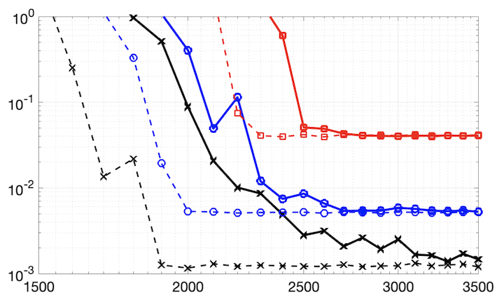
Figure 1: Log-scale plot of average relative error for Algorithm 1 as a function of the number of nodes $n$ in each RVFL network. Black (cross), blue (circle), and red (square) lines correspond to GMRA refinement levels $j=12$, $j=9$, and $j=6$ (resp.). For each $j$, we fix $\alpha_{j}=2$ and vary $\Omega_{j}=10,15$ (solid and dashed lines, resp.). Reconstruction error decays as a function of $n$ until reaching a floor due to error in the GMRA approximation of $\mathcal{M}$.

Appendix A Proofs

A.1 Proof of Lemma 3.3

Observe that $h_{\Omega}$ defined in (3) may be viewed as a multidimensional bump function; indeed, the parameter $\Omega>0$ controls the width of the bump. In particular, if $\Omega$ is allowed to grow very large, then $h_{\Omega}$ becomes very localized near the origin. Objects that behave in this way are known in the functional analysis literature as approximate $\delta$-functions:

Definition A.1.

A sequence of functions $\{\varphi_{t}\}_{t>0}\subset L^{1}(\mathbb{R}^{N})$ are called approximate (or nascent) $\delta$-functions if

$$\lim_{t\rightarrow\infty}\int_{\mathbb{R}^{N}}\varphi_{t}(x)f(x)\mathrm{d}x=f(0)$$

for all $f\in C_{c}(\mathbb{R}^{N})$. For such functions, we write $\delta_{0}(x)=\lim_{t\rightarrow\infty}\varphi_{t}(x)$ for all $x\in\mathbb{R}^{N}$, where $\delta_{0}$ denotes the $N$-dimensional Dirac $\delta$-function centered at the origin.

Given $\varphi\in L^{1}(\mathbb{R}^{N})$ with $\int_{\mathbb{R}^{N}}\varphi(x)\mathrm{d}x=1$, one may construct approximate $\delta$-functions for $t>0$ by defining $\varphi_{t}(x):=t^{N}\varphi(tx)$ for all $x\in\mathbb{R}^{N}$ (Stein and Weiss, 1971). Such sequences of approximate $\delta$-functions are also called approximate identity sequences (Rudin, 1991) since they satisfy a particularly nice identity with respect to convolution, namely, $\lim_{t\rightarrow\infty}\|f*\varphi_{t}-f\|_{1}=0$ for all $f\in C_{c}(\mathbb{R}^{N})$ (see Rudin, 1991, Theorem 6.32). In fact, such an identity holds much more generally.

Lemma A.2.

(Stein and Weiss, 1971, Theorem 1.18) Let $\varphi\in L^{1}(\mathbb{R}^{N})$ with $\int_{\mathbb{R}^{N}}\varphi(x)\mathrm{d}x=1$ and for $t>0$ define $\varphi_{t}(x):=t^{N}\varphi(tx)$ for all $x\in\mathbb{R}^{N}$. If $f\in L^{p}(\mathbb{R}^{N})$ for $1\leq p<\infty$ (or $f\in C_{0}(\mathbb{R}^{N})\subset L^{\infty}(\mathbb{R}^{N})$ for $p=\infty$), then $\lim_{t\rightarrow\infty}\|f*\varphi_{t}-f\|_{p}=0$.

To prove (4), it would suffice to have $\lim_{\Omega\to\infty}\lVert f*h_{\Omega}-f\rVert_{\infty}=0,$ which is really just Lemma A.2 in case $p=\infty.$ Nonetheless, we present a proof by mimicking Stein and Weiss (1971) for completeness. Moreover, we will use a part of proof in Remark A.5 below.

Lemma A.3.

Let $h\in L^{1}(\mathbb{R}^{n})$ with $\int_{\mathbb{R}^{N}}h(x)\mathrm{d}x=1$ and define $h_{\Omega}\in L^{1}(\mathbb{R}^{N})$ as in (3) for all $\Omega>0.$ Then, for all $f\in C_{0}(\mathbb{R}^{N})$, we have

$$\lim_{\Omega\to\infty}\sup_{x\in\mathbb{R}^{N}}\big{\lvert}(f*h_{\Omega})(x)-f(x)\big{\rvert}=0.$$

Proof A.4.

By symmetry of the convolution operator in its arguments, we have

$$\sup_{x\in\mathbb{R}^{N}}\big{\lvert}(f*h_{\Omega})(x)-f(x)\big{\rvert} =\sup_{x\in\mathbb{R}^{N}}\Big{\lvert}\int_{\mathbb{R}^{N}}f(y)h_{\Omega}(x-y)\mathrm{d}y-f(x)\Big{\rvert}$$

$$=\sup_{x\in\mathbb{R}^{N}}\Big{\lvert}\int_{\mathbb{R}^{N}}f(x-y)h_{\Omega}(y)\mathrm{d}y-f(x)\Big{\rvert}.$$

Since a simple substitution yields $1=\int_{\mathbb{R}^{N}}h(x)\mathrm{d}x=\int_{\mathbb{R}^{N}}h_{\Omega}(x)\mathrm{d}x,$ it follows that

$$\sup_{x\in\mathbb{R}^{N}}\big{\lvert}(f*h_{\Omega})(x)-f(x)\big{\rvert} =\sup_{x\in\mathbb{R}^{N}}\Big{\lvert}\int_{\mathbb{R}^{N}}\big{(}f(x-y)-f(x)\big{)}h_{\Omega}(y)\mathrm{d}y\Big{\rvert}$$

$$\leq\int_{\mathbb{R}^{N}}\lvert h_{\Omega}(y)\rvert\sup_{x\in\mathbb{R}^{N}}\big{\lvert}f(x)-f(x-y)\big{\rvert}\mathrm{d}y.$$

Finally, expanding the function $h_{\Omega},$ we obtain

$$\sup_{x\in\mathbb{R}^{N}}\big{\lvert}(f*h_{\Omega})(x)-f(x)\big{\rvert} \leq\int_{\mathbb{R}^{N}}\Big{(}\Omega^{N}\lvert h(\Omega y)\rvert\Big{)}\sup_{x\in\mathbb{R}^{N}}\big{\lvert}f(x)-f(x-y)\big{\rvert}\mathrm{d}y$$

$$=\int_{\mathbb{R}^{N}}\lvert h(z)\rvert\sup_{x\in\mathbb{R}^{N}}\big{\lvert}f(x)-f(x-z/\Omega)\big{\rvert}\mathrm{d}z,$$

where we have used the substitution $z=\Omega y.$ Taking limits on both sides of this expression and observing that

$$\int_{\mathbb{R}^{N}}\lvert h(z)\rvert\sup_{x\in\mathbb{R}^{N}}\big{\lvert}f(x)-f(x-z/\Omega)\big{\rvert}\mathrm{d}z\leq 2\lVert h\rVert_{1}\sup_{x\in\mathbb{R}^{N}}\lvert f(x)\rvert<\infty,$$

using the Dominated Convergence Theorem, we obtain

$$\lim_{\Omega\to\infty}\sup_{x\in\mathbb{R}^{N}}\big{\lvert}(f*h_{\Omega})(x)-f(x)\big{\rvert}\leq\int_{\mathbb{R}^{N}}\lvert h(z)\rvert\lim_{\Omega\to\infty}\sup_{x\in\mathbb{R}^{N}}\big{\lvert}f(x)-f(x-z/\Omega)\big{\rvert}\mathrm{d}z.$$

So, it suffices to show that, for all $z\in\mathbb{R}^{N}$,

$$\lim_{\Omega\to\infty}\sup_{x\in\mathbb{R}^{N}}\big{\lvert}f(x)-f(x-z/\Omega)\big{\rvert}=0.$$

To this end, let $\varepsilon>0$ and $z\in\mathbb{R}^{N}$ be arbitrary. Since $f\in C_{0}(\mathbb{R}^{N})$, there exists $r>0$ sufficiently large such that $|f(x)|<\varepsilon/2$ for all $x\in\mathbb{R}^{N}\setminus\overline{B(0,r)}$, where $\overline{B(0,r)}\subset\mathbb{R}^{N}$ is the closed ball of radius $r$ centered at the origin. Let $\mathcal{B}:=\overline{B(0,r+\lVert z/\Omega\rVert_{2})},$ so that for each $x\in\mathbb{R}^{N}\setminus\mathcal{B}$ we have both $x$ and $x-z/\Omega$ in $\mathbb{R}^{N}\setminus\overline{B(0,r)}$. Thus, both $|f(x)|<\varepsilon/2$ and $\lvert f(x-z/\Omega)\rvert<\varepsilon/2,$ implying that

$$\sup_{x\in\mathbb{R}^{N}\setminus\mathcal{B}}\big{\lvert}f(x)-f(x-z/\Omega)\big{\rvert}<\varepsilon.$$

Hence, we obtain

$$\lim_{\Omega\to\infty}\sup_{x\in\mathbb{R}^{N}}\big{\lvert}f(x)-f(x-z/\Omega)\big{\rvert}$$

$$\quad\leq\lim_{\Omega\to\infty}\max\Big{\{}\sup_{x\in\mathcal{B}}\big{\lvert}f(x)-f(x-z/\Omega)\big{\rvert},\sup_{x\in\mathbb{R}^{N}\setminus\mathcal{B}}\big{\lvert}f(x)-f(x-z/\Omega)\big{\rvert}\Big{\}}$$

$$\quad\leq\max\Big{\{}\varepsilon,\lim_{\Omega\to\infty}\sup_{x\in\mathcal{B}}\big{\lvert}f(x)-f(x-z/\Omega)\big{\rvert}\Big{\}}.$$

Now, as $\mathcal{B}$ is a compact subset of $\mathbb{R}^{N}$, the continuous function $f$ is uniformly continuous on $\mathcal{B}$, and so the remaining limit and supremum may be freely interchanged, whereby continuity of $f$ yields

$$\lim_{\Omega\to\infty}\sup_{x\in\mathcal{B}}\big{\lvert}f(x)-f(x-z/\Omega)\big{\rvert}=\sup_{x\in\mathcal{B}}\lim_{\Omega\to\infty}\big{\lvert}f(x)-f(x-z/\Omega)\big{\rvert}=0.$$

Since $\varepsilon>0$ may be taken arbitrarily small, we have proved the result.

Remark A.5.

While Lemma A.3 does the approximation we aim for, it gives no indication of how fast

$$\sup_{x\in\mathbb{R}^{N}}\big{\lvert}(f*h_{\Omega})(x)-f(x)\big{\rvert}$$

decays in terms of $\Omega$ or the dimension $N.$ Assuming $h(z)=g(z(1))\cdots g(z(N))$ for some nonnegative $g$ (which is how we will choose $h$ in Section A.2) and $f$ to be $\beta$-Hölder continuous for some fixed $\beta\in(0,1)$ yields that

$$\sup_{x\in\mathbb{R}^{N}}\big{\lvert}(f*h_{\Omega})(x)-f(x)\big{\rvert} \leq\int_{\mathbb{R}^{N}}\lvert h(z)\rvert\sup_{x\in\mathbb{R}^{N}}\big{\lvert}f(x)-f(x-z/\Omega)\big{\rvert}\mathrm{d}z$$

$$\lesssim\Omega^{-\beta}\int_{\mathbb{R}^{N}}\lVert z\rVert_{2}^{\beta}h(z)\mathrm{d}z$$

$$\leq\Omega^{-\beta}\bigg{(}\int_{\mathbb{R}^{N}}\Big{(}z(1)^{2}+\cdots+z(N)^{2}\Big{)}h(z)\mathrm{d}z\bigg{)}^{\beta/2}$$

$$\leq\Omega^{-\beta}\bigg{(}N\max_{j\in\{1,\ldots,N\}}\int_{\mathbb{R}^{N}}z(j)^{2}h(z)\mathrm{d}z\bigg{)}^{\beta/2}$$

$$=(\sqrt{N}/\Omega)^{\beta}\bigg{(}\max_{j\in\{1,\ldots,N\}}\int_{\mathbb{R}}z(j)^{2}g(z(j))\mathrm{d}z(j)\bigg{)}^{\beta/2}$$

$$=(\sqrt{N}/\Omega)^{\beta}\bigg{(}\int_{\mathbb{R}}z(1)^{2}g(z(1))\mathrm{d}z(1)\bigg{)}^{\beta/2}$$

$$\lesssim(\sqrt{N}/\Omega)^{\beta}$$

where the third inequality follows from Jensen’s inequality. One can, with appropriate changes, extend this result to homogeneous Hölder–Zygmund functions of any order.

A.2 Proof of 3.4: The limit-integral representation

Let $A\in C^{\infty}(\mathbb{R})$ be any even function supported on $[-\tfrac{1}{2},\tfrac{1}{2}]$ s.t. $\lVert A\rVert_{2}=1.$ Then $\phi=A*A\in C^{\infty}(\mathbb{R})$ is an even function supported on $[-1,1]$ s.t. $\phi(0)=1.$ Lemma 3.3 implies that

$$f(x)=\lim_{\Omega\to\infty}(f*h_{\Omega})(x)$$ (24)

uniformly in $x\in K$ for any $h\in L^{1}(\mathbb{R}^{N})$ satisfying $\int_{\mathbb{R}^{N}}h(z)\mathrm{d}z=1.$ We choose

$$h(z)=\frac{1}{(2\pi)^{N}}\int_{\mathbb{R}^{N}}\exp(i\langle w,z\rangle)\prod_{j=1}^{N}\phi(w(j))\mathrm{d}w$$

which the reader may recognize as the (inverse) Fourier transform of $\prod_{j=1}^{N}\phi(w(j))$. As we announced in Remark A.5, $h(z)=g(z(1))\cdots g(z(N)),$ where (using the convolution theorem)

$$g(z(j)) =\frac{1}{2\pi}\int_{\mathbb{R}}\exp(iw(j)z(j))\phi(w(j))\mathrm{d}w(j)$$

$$=\frac{1}{2\pi}\int_{\mathbb{R}}\exp(iw(j)z(j))(A*A)(w(j))\mathrm{d}w(j)$$

$$=2\pi\bigg{(}\frac{1}{2\pi}\int_{\mathbb{R}}\exp(iw(j)z(j))A(w(j))\mathrm{d}w(j)\bigg{)}^{2}\geq 0$$

Moreover, since $g$ is the Fourier transform of an even function, $h$ is real-valued and even as well. In addition, since $\phi$ is smooth, $h$ decays faster than the reciprocal of any polynomial (which follows from repeated integration by parts and the Riemann–Lebesgue lemma), so a fortiori $h\in L^{1}(\mathbb{R}^{N}).$ Therefore, Fourier inversion yields that

$$\int_{\mathbb{R}^{N}}h(z)\mathrm{d}z=\int_{\mathbb{R}^{N}}\exp(-i\langle w,z\rangle)h(z)\mathrm{d}z\Big{\rvert}_{w=0}=\prod_{j=1}^{N}\phi(0)=1$$

which justifies our application of Lemma 3.3. Expanding the right-hand side of (24) (using the scaling property of the Fourier transform) yields that

$$(f*h_{\Omega})(x) =\int_{\mathbb{R}^{N}}f(y)h_{\Omega}(x-y)\mathrm{d}y=\frac{1}{(2\pi)^{N}}\int_{K}f(y)\int_{\mathbb{R}^{N}}\exp(i\langle w,x-y\rangle)\prod_{j=1}^{N}\phi(w(j)/\Omega)\mathrm{d}w\mathrm{d}y$$

$$=\frac{1}{(2\pi)^{N}}\int_{K}\int_{[-\Omega,\Omega]^{N}}f(y)\cos(\langle w,x-y\rangle)\prod_{j=1}^{N}\phi(w(j)/\Omega)\mathrm{d}w\mathrm{d}y$$ (25)

because $\phi$ is even and supported on $[-1,1].$ Since (25) is an iterated integral of a continuous function over a compact set, Fubini’s theorem readily applies, yielding

$$f(x)=\lim_{\Omega\to\infty}(f*h_{\Omega})(x)=\lim_{\Omega\to\infty}\frac{1}{(2\pi)^{N}}\int_{K\times[-\Omega,\Omega]^{N}}f(y)\cos(\langle w,x-y\rangle)\prod_{j=1}^{N}\phi(w(j)/\Omega)\mathrm{d}y\mathrm{d}w$$

Since $\lvert\langle w,x-y\rangle\rvert\leq\lVert x-y\rVert_{1}\lVert w\rVert_{\infty}\leq 2N\mathrm{rad}(K)\Omega\leq(L+\tfrac{1}{2})\pi,$ it follows that

$$f(x)=\lim_{\Omega\to\infty}\frac{1}{(2\pi)^{N}}\int_{K\times[-\Omega,\Omega]^{N}}f(y)\cos_{\Omega}(\langle w,x-y\rangle)\prod_{j=1}^{N}\phi(w(j)/\Omega)\mathrm{d}y\mathrm{d}w$$ (26)

where $\cos_{\Omega}$ is defined in (5).

With the representation (26) in hand, we now seek to reintroduce the general activation function $\rho$. To this end, since $\cos_{\Omega}\in C_{c}(\mathbb{R})\subset C_{0}(\mathbb{R})$ we may apply the convolution identity (4) with $f$ replaced by $\cos_{\Omega}$ to obtain $\cos_{\Omega}(z)=\lim_{\alpha\rightarrow\infty}(\cos_{\Omega}*h_{\alpha})(z)$ uniformly for all $z\in\mathbb{R}$, where $h_{\alpha}(z)=\alpha\rho(\alpha z).$ Using this representation of $\cos_{\Omega}$ in (26), it follows that

$$f(x)=\lim_{\Omega\rightarrow\infty}\frac{1}{(2\Omega)^{N}}\int_{K\times[-\Omega,\Omega]^{N}}f(y)\Big{(}\lim_{\alpha\rightarrow\infty}\big{(}\cos_{\Omega}*h_{\alpha}\big{)}\big{(}\langle w,x-y\rangle\big{)}\Big{)}\prod_{j=1}^{N}\phi(w(j)/\Omega)\mathrm{d}y\mathrm{d}w$$

holds uniformly for all $x\in K$. Since $f$ is continuous and the convolution $\cos_{\Omega}*h_{\alpha}$ is uniformly continuous and uniformly bounded in $\alpha$ by $\lVert\rho\rVert_{1}$ (see below), the fact that the domain $K\times[-\Omega,\Omega]^{N}$ is compact then allows us to bring the limit as $\alpha$ tends to infinity outside the integral in this expression via the Dominated Convergence Theorem, which gives us

$$f(x)=\lim_{\Omega\rightarrow\infty}\lim_{\alpha\rightarrow\infty}\frac{1}{(2\Omega)^{N}}\int_{K\times[-\Omega,\Omega]^{N}}f(y)\big{(}\cos_{\Omega}*h_{\alpha}\big{)}\big{(}\langle w,x-y\rangle\big{)}\prod_{j=1}^{N}\phi(w(j)/\Omega)\mathrm{d}y\mathrm{d}w$$ (27)

uniformly for every $x\in K$. The uniform boundedness of the convolution follows from the fact that

$$(\cos_{\Omega}*h_{\alpha})(z)=\int_{\mathbb{R}}\cos_{\Omega}(z-u)h_{\alpha}(u)\mathrm{d}u=\int_{\mathbb{R}}\cos_{\Omega}(z-v/\alpha)\rho(v)\mathrm{d}v$$

where $v=\alpha u.$

Remark A.6.

It should be noted that we are unable to swap the order of the limits in (27) since $\cos_{\Omega}$ is not in $C_{0}(\mathbb{R})$ when $\Omega$ is allowed to be infinite.

To complete this step of the proof, observe that the definition of $\cos_{\Omega}$ allows us to write

$$(\cos_{\Omega}*h_{\alpha})(z)=\alpha\int_{\mathbb{R}}\cos_{\Omega}(u)\rho\big{(}\alpha(z-u)\big{)}\mathrm{d}u=\alpha\int_{-\frac{\pi}{2}(2L+1)}^{\frac{\pi}{2}(2L+1)}\cos_{\Omega}(u)\rho\big{(}\alpha(z-u)\big{)}\mathrm{d}u$$ (28)

By substituting (28) into (27), we then obtain

$$f(x)=\lim_{\Omega\rightarrow\infty}\lim_{\alpha\rightarrow\infty}\frac{\alpha}{(2\pi)^{N}}\int_{K(\Omega)}f(y)\cos_{\Omega}(u)\rho\Big{(}\alpha\big{(}\langle w,x-y\rangle-u\big{)}\Big{)}\prod_{j=1}^{N}\phi(w(j)/\Omega)\mathrm{d}y\mathrm{d}w\mathrm{d}u$$

uniformly for all $x\in K$, where $K(\Omega):=K\times[-\Omega,\Omega]^{N}\times[-\frac{\pi}{2}(2L+1),\frac{\pi}{2}(2L+1)]$. In this way, recalling that $F_{\alpha,\Omega}(y,w,u):=\frac{\alpha}{(2\pi)^{N}}f(y)\cos_{\Omega}(u)\prod_{j=1}^{N}\phi(w(j)/\Omega),$ and $b_{\alpha}(y,w,u):=-\alpha(\langle w,y\rangle+u)$ for $y,w\in\mathbb{R}^{N}$ and $u\in\mathbb{R}$, we conclude the proof.

A.3 Proof of Lemma 3.5: Monte-Carlo integral approximation

The next step in the proof of Theorem 3.1 is to approximate the integral in (7) using the Monte-Carlo method. To this end, let $\{y_{k}\}_{k=1}^{n}$, $\{w_{k}\}_{k=1}^{n}$, and $\{u_{k}\}_{k=1}^{n}$ be independent samples drawn uniformly from $K$, $[-\Omega,\Omega]^{N}$, and $[-\frac{\pi}{2}(2L+1),\frac{\pi}{2}(2L+1)]$, respectively, and consider the sequence of random variables $\{I_{n}(x)\}_{n=1}^{\infty}$ defined by

$$I_{n}(x):=\frac{\mathrm{vol}(K(\Omega))}{n}\sum_{k=1}^{n}F_{\alpha,\Omega}(y_{k},w_{k},u_{k})\rho\big{(}\alpha\langle w_{k},x\rangle+b_{\alpha}(y_{k},w_{k},u_{k})\big{)}$$ (29)

for each $x\in K$, where we note that $\mathrm{vol}(K(\Omega))=(2\Omega)^{N}\pi(2L+1)\mathrm{vol}(K)$. If we also define

$$I(x;p):=\int_{K(\Omega)}\Big{(}F_{\alpha,\Omega}(y,w,u)\rho\big{(}\alpha\langle w,x\rangle+b_{\alpha}(y,w,u)\big{)}\Big{)}^{p}\mathrm{d}y\mathrm{d}w\mathrm{d}u$$ (30)

for $x\in K$ and $p\in\mathbb{N}$, then we want to show that

$$\mathbb{E}\int_{K}|I(x;1)-I_{n}(x)|^{2}\mathrm{d}x=O(1/n)$$ (31)

as $n\to\infty,$ where the expectation is taken with respect to the joint distribution of the random samples $\{y_{k}\}_{k=1}^{n}$, $\{w_{k}\}_{k=1}^{n}$, and $\{u_{k}\}_{k=1}^{n}$. For this, it suffices to find a constant $C(f,\rho,\alpha,\Omega,N)<\infty$ independent of $n$ satisfying

$$\int_{K}\mathbb{E}|I(x;1)-I_{n}(x)|^{2}\mathrm{d}x\leq\frac{C(f,\rho,\alpha,\Omega,N)}{n}.$$

Indeed, an application of Fubini’s theorem would then yield

$$\mathbb{E}\int_{K}|I(x;1)-I_{n}(x)|^{2}\mathrm{d}x\leq\frac{C(f,\rho,\alpha,\Omega,N)}{n},$$

which implies (31). To determine such a constant, we first observe by Theorem 2.1 that

$$\mathbb{E}|I(x;1)-I_{n}(x)|^{2}=\frac{\mathrm{vol}^{2}(K(\Omega))\sigma(x)^{2}}{n},$$

where we define the variance term

$$\sigma(x)^{2}:=\frac{I(x;2)}{\mathrm{vol}(K(\Omega))}-\frac{I(x;1)^{2}}{\mathrm{vol}^{2}(K(\Omega))}$$

for $x\in K$. Since $\lVert\phi\rVert_{\infty}=1$ (see Lemma A.7 below), it follows that

$$\lvert F_{\alpha,\Omega}(y,w,u)\rvert =\frac{\alpha}{(2\pi)^{N}}\lvert f(y)\rvert\cdot\lvert\cos_{\Omega}(u)\rvert\prod_{j=1}^{N}\lvert\phi(w(j)/\Omega)\rvert\leq\frac{\alpha M}{(2\pi)^{N}}$$

for all $y,w\in\mathbb{R}^{N}$ and $u\in\mathbb{R}$, where $M:=\sup_{x\in K}|f(x)|<\infty$, we obtain the following simple bound on the variance term

$$\sigma(x)^{2}\leq\frac{I(x;2)}{\mathrm{vol}(K(\Omega))}\leq\frac{\alpha^{2}M^{2}}{(2\pi)^{2N}\mathrm{vol}(K(\Omega))}\int_{K(\Omega)}\Big{|}\rho\big{(}\alpha\langle w,x\rangle+b_{\alpha}(y,w,u)\big{)}\Big{|}^{2}\mathrm{d}y\mathrm{d}w\mathrm{d}u.$$ (32)

Since we assume $\rho\in L^{\infty}(\mathbb{R}),$ we then have

$$\int_{K}\mathbb{E}|I(x;1)-I_{n}(x)|^{2}\mathrm{d}x =\frac{\mathrm{vol}^{2}(K(\Omega))}{n}\int_{K}\sigma(x)^{2}\mathrm{d}x$$

$$\leq\frac{\alpha^{2}M^{2}\mathrm{vol}(K(\Omega))}{(2\pi)^{2N}n}\int_{K\times K(\Omega)}\Big{|}\rho\big{(}\alpha\langle w,x\rangle+b_{\alpha}(y,w,u)\big{)}\Big{|}^{2}\mathrm{d}x\mathrm{d}y\mathrm{d}w\mathrm{d}u$$

$$=\frac{\alpha^{2}M^{2}\mathrm{vol}^{2}(K(\Omega))\mathrm{vol}(K)\lVert\rho\rVert_{\infty}^{2}}{(2\pi)^{2N}n}.$$

Substituting the value of $\mathrm{vol}(K(\Omega))$, we obtain

$$C(f,\rho,\alpha,\Omega,N):=\alpha^{2}M^{2}(\Omega/\pi)^{2N}\pi^{2}(2L+1)^{2}\mathrm{vol}^{3}(K)\|\rho\|_{\infty}^{2}$$

is a suitable choice for the desired constant.

Now that we have established (31), we may rewrite the random variables $I_{n}(x)$ in a more convenient form. To this end, we change the domain of the random samples $\{w_{k}\}_{k=1}^{n}$ to $[-\alpha\Omega,\alpha\Omega]^{N}$ and define the new random variables $\{b_{k}\}_{k=1}^{n}\subset\mathbb{R}$ by $b_{k}:=-(\langle w_{k},y_{k}\rangle+\alpha u_{k})$ for each $k=1,\ldots,n$. In this way, if we denote

$$v_{k}:=\frac{\mathrm{vol}(K(\Omega))}{n}F_{\alpha,\Omega}\Big{(}y_{k},\frac{w_{k}}{\alpha},u_{k}\Big{)}$$

for each $k=1,\ldots,n$, the random variables $\{f_{n}\}_{n=1}^{\infty}$ defined by

$$f_{n}(x):=\sum_{k=1}^{n}v_{k}\rho\big{(}\langle w_{k},x\rangle+b_{k}\big{)}$$

satisfy $f_{n}(x)=I_{n}(x)$ for every $x\in K$. Combining this with (31), we have proved Lemma 3.5.

Lemma A.7.

$\lVert\phi\rVert_{\infty}=1.$

Proof A.8.

It suffices to prove that $\lvert\phi(z)\rvert\leq 1$ for all $z\in\mathbb{R}$ because $\phi(0)=1.$ By Cauchy–Schwarz,

$$\lvert\phi(z)\rvert =\bigg{\lvert}\int_{\mathbb{R}}A(u)A(z-u)\mathrm{d}u\bigg{\rvert}\leq\sqrt{\int_{\mathbb{R}}\displaystyle A(u)A(u)\mathrm{d}u\int_{\mathbb{R}}\displaystyle A(z-u)A(z-u)\mathrm{d}u}$$

$$=\sqrt{\int_{\mathbb{R}}\displaystyle A(u)A(0-u)\mathrm{d}u\int_{\mathbb{R}}\displaystyle A(v)A(-v)\mathrm{d}v}=\sqrt{\phi(0)\phi(0)}=1$$

because $A$ is even.

A.4 Proof of Theorem 1.1 when $\rho^{\prime}\in L^{1}(\mathbb{R})\cap L^{\infty}(\mathbb{R})$

Let $f\in C_{c}(\mathbb{R}^{N})$ with $K:=\mathrm{supp}(f)$ and suppose $\varepsilon>0$ is fixed. Take the activation function $\rho\colon\mathbb{R}\rightarrow\mathbb{R}$ to be differentiable with $\rho^{\prime}\in L^{1}(\mathbb{R})\cap L^{\infty}(\mathbb{R}).$ We wish to show that there exists a sequence of RVFL networks $\{f_{n}\}_{n=1}^{\infty}$ defined on $K$ which satisfy the asymptotic error bound

$$\mathbb{E}\int_{K}|f(x)-f_{n}(x)|^{2}\mathrm{d}x\leq\varepsilon+O(1/n)$$

as $n\to\infty.$ The proof of this result is a minor modification of second step in the proof of Theorem 3.1.

If we redefine $h_{\alpha}(z)$ as $\alpha\rho^{\prime}(\alpha z),$ then (27) plainly still holds and (28) reads

$$(\cos_{\Omega}*h_{\alpha})(z)=\alpha\int_{\mathbb{R}}\cos_{\Omega}(u)\rho^{\prime}\big{(}\alpha(z-u)\big{)}\mathrm{d}u.$$

Recalling the definition of $\cos_{\Omega}$ in (5) and integrating by parts, we obtain

$$(\cos_{\Omega}*h_{\alpha})(z) =\alpha\int_{\mathbb{R}}\cos_{\Omega}(u)\rho^{\prime}\big{(}\alpha(z-u)\big{)}\mathrm{d}u$$

$$=-\int_{-\frac{\pi}{2}(2L+1)}^{\frac{\pi}{2}(2L+1)}\cos_{\Omega}(u)d\rho(\alpha(z-u))$$

$$=-\cos_{\Omega}(u)\rho(\alpha(z-u))\Big{|}_{-\frac{\pi}{2}(2L+1)}^{\frac{\pi}{2}(2L+1)}+\int_{-\frac{\pi}{2}(2L+1)}^{\frac{\pi}{2}(2L+1)}\rho(\alpha(z-u))d\cos_{\Omega}(u)$$

$$=-\int_{\mathbb{R}}\sin_{\Omega}(u)\rho\big{(}\alpha(z-u)\big{)}\mathrm{d}u$$

for all $z\in\mathbb{R}$, where $L:=\lceil\frac{2N}{\pi}\mathrm{rad}(K)\Omega-\frac{1}{2}\rceil$ and $\sin_{\Omega}\colon\mathbb{R}\rightarrow[-1,1]$ is defined analogously to (5). Substituting this representation of $(\cos_{\Omega}*h_{\alpha})(z)$ into (27) then yields

$$f(x)=\lim_{\Omega\rightarrow\infty}\lim_{\alpha\rightarrow\infty}\frac{-\alpha}{(2\pi)^{N}}\int_{K(\Omega)}f(y)\sin_{\Omega}(u)\rho\big{(}\alpha(\langle w,x-y\rangle-u)\big{)}\prod_{j=1}^{N}\phi(w(j)/\Omega)\mathrm{d}y\mathrm{d}w\mathrm{d}u$$

uniformly for every $x\in K$. Thus, if we replace the definition of $F_{\alpha,\Omega}$ in (6) by

$$F_{\alpha,\Omega}(y,w,u) :=\frac{-\alpha}{(2\pi)^{N}}f(y)\sin_{\Omega}(u)\prod_{j=1}^{N}\phi(w(j)/\Omega)$$

for $y,w\in\mathbb{R}^{N}$ and $u\in\mathbb{R}$, we again obtain the uniform representation (7) for all $x\in K$. The remainder of the proof proceeds from this point exactly as in the proof of Theorem 3.1.

A.5 Proof of Theorem 5.4

We wish to show that there exist sequences of RVFL networks $\{\tilde{f}_{n_{j}}\}_{n_{j}=1}^{\infty}$ defined on $\phi_{j}(U_{j})$ for each $j\in J$ which together satisfy the error bound

$$\int_{\mathcal{M}}\bigg{|}f(x)\quad-\sum_{\{j\in J\colon x\in U_{j}\}}(\tilde{f}_{n_{j}}\circ\phi_{j})(x)\bigg{|}^{2}\mathrm{d}x<\varepsilon$$

with probability at least $1-\eta$ when $\{n_{j}\}_{j\in J}$ are chosen sufficiently large. The proof is obtained by showing that

$$\bigg{|}f(x)\quad-\sum_{\{j\in J\colon x\in U_{j}\}}(\tilde{f}_{n_{j}}\circ\phi_{j})(x)\bigg{|}<\sqrt{\frac{\varepsilon}{\mathrm{vol}(\mathcal{M})}}$$ (33)

holds uniformly for $x\in\mathcal{M}$ with high probability.

We begin as in the proof of Theorem 5.1 by applying the representation (17) for $f$ on each chart $(U_{j},\phi_{j})$, which gives us

$$\bigg{|}f(x)\quad-\sum_{\{j\in J\colon x\in U_{j}\}}(\tilde{f}_{n_{j}}\circ\phi_{j})(x)\bigg{|} \leq\sum_{\{j\in J\colon x\in U_{j}\}}\Big{|}(\hat{f}_{j}\circ\phi_{j})(x)-(\tilde{f}_{n_{j}}\circ\phi_{j})(x)\Big{|}$$ (34)

for all $x\in\mathcal{M}$. Now, since we have already seen that $\hat{f}_{j}\in C_{c}(\mathbb{R}^{d})$ for each $j\in J$, Theorem 4.1 implies that for any $\varepsilon_{j}>0$, there exist constants $\alpha_{j},\Omega_{j}>0$ and hidden-to-output layer weights $\{v_{k}^{(j)}\}_{k=1}^{n_{j}}\subset\mathbb{R}$ for each $j\in J$ such that for any

$$\delta_{j}<\frac{\sqrt{\varepsilon_{j}}}{8\sqrt{2d}\kappa\alpha_{j}^{2}M_{j}\Omega_{j}(\Omega_{j}/\pi)^{d}\mathrm{vol}^{3/2}(\phi_{j}(U_{j}))(\pi+2d\mathrm{rad}(\phi_{j}(U_{j}))\Omega)}$$ (35)

we have

$$\Big{|}\hat{f}_{j}(z)-\tilde{f}_{n_{j}}(z)\Big{|}<\sqrt{\frac{\varepsilon_{j}}{2\mathrm{vol}(\phi_{j}(U_{j}))}}$$

uniformly for all $z\in\phi_{j}(U_{j})$ with probability at least $1-\eta_{j}$, provided the number of nodes $n_{j}$ satisfies

$$n_{j} \geq\frac{c\Sigma^{(j)}\alpha_{j}(\Omega_{j}/\pi)^{d}(\pi+2d\mathrm{rad}(\phi_{j}(U_{j}))\Omega_{j})\log(3\eta_{j}^{-1}\mathcal{N}(\delta_{j},\phi_{j}(U_{j})))}{\sqrt{\varepsilon_{j}}\log\big{(}1+\frac{\sqrt{\varepsilon_{j}}}{\Sigma^{(j)}\alpha_{j}(\Omega_{j}/\pi)^{d}(\pi+2d\mathrm{rad}(\phi_{j}(U_{j}))\Omega_{j})}\big{)}},$$ (36)

where $c>0$ is a numerical constant and $\Sigma^{(j)}:=2C^{(j)}\sqrt{2\mathrm{vol}(\phi_{j}(U_{j}))}.$ Indeed, it suffices to choose

$$v_{k}^{(j)} :=\frac{\mathrm{vol}(K(\Omega_{j}))}{n_{j}}F_{\alpha_{j},\Omega_{j}}\Big{(}y_{k}^{(j)},\frac{w_{k}^{(j)}}{\alpha_{j}},u_{k}^{(j)}\Big{)}$$

for each $k=1,\ldots,n_{j}$, where

$$K(\Omega_{j}):=\phi_{j}(U_{j})\times[-\alpha_{j}\Omega_{j},\alpha_{j}\Omega_{j}]^{d}\times[-\tfrac{\pi}{2}(2L_{j}+1),\tfrac{\pi}{2}(2L_{j}+1)]$$

for each $j\in J$. Combined with (34), choosing $\delta_{j}$ and $n_{j}$ satifying (35) and (36), respectively, then yields

$$\bigg{|}f(x)\quad-\sum_{\{j\in J\colon x\in U_{j}\}}(\tilde{f}_{n_{j}}\circ\phi_{j})(x)\bigg{|} <\sum_{\{j\in J\colon x\in U_{j}\}}\sqrt{\frac{\varepsilon_{j}}{2\mathrm{vol}(\phi_{j}(U_{j}))}}\leq\sum_{j\in J}\sqrt{\frac{\varepsilon_{j}}{2\mathrm{vol}(\phi_{j}(U_{j}))}}$$

for all $x\in\mathcal{M}$ with probability at least $1-\sum_{\{j\in J\colon x\in U_{j}\}}\eta_{j}\geq 1-\sum_{j\in J}\eta_{j}$. Since we require that (33) holds for all $x\in\mathcal{M}$ with probability at least $1-\eta$, the proof is then completed by choosing $\{\varepsilon_{j}\}_{j\in J}$ and $\{\eta_{j}\}_{j\in J}$ such that

$$\varepsilon=\frac{\mathrm{vol}(\mathcal{M})}{2}\Big{(}\sum_{j\in J}\sqrt{\frac{\varepsilon_{j}}{\mathrm{vol}(\phi_{j}(U_{j}))}}\Big{)}^{2}\quad\text{ and }\quad\eta=\sum_{j\in J}\eta_{j}.$$

In particular, it suffices to choose

$$\varepsilon_{j}=\frac{2\mathrm{vol}(\phi_{j}(U_{j}))\,\varepsilon}{|J|^{2}\mathrm{vol}(\mathcal{M})}$$

and $\eta_{j}=\eta/|J|$ for each $j\in J$, so that (35) and (36) become

$$\delta_{j} <\frac{\sqrt{\varepsilon}}{8\lvert J\rvert\sqrt{d\mathrm{vol}(\mathcal{M})}\kappa\alpha_{j}^{2}M_{j}\Omega_{j}(\Omega_{j}/\pi)^{d}\mathrm{vol}(\phi_{j}(U_{j}))(\pi+2d\mathrm{rad}(\phi_{j}(U_{j}))\Omega)},$$

$$n_{j} \geq\frac{2c\lvert J\rvert\sqrt{\mathrm{vol}(\mathcal{M})}C^{(j)}\alpha_{j}(\Omega_{j}/\pi)^{d}(\pi+2d\mathrm{rad}(\phi_{j}(U_{j}))\Omega_{j})\log(3\lvert J\rvert\eta^{-1}\mathcal{N}(\delta_{j},\phi_{j}(U_{j})))}{\sqrt{\varepsilon}\log\big{(}1+\frac{\sqrt{\varepsilon}}{2\lvert J\rvert\sqrt{\mathrm{vol}(\mathcal{M})}C^{(j)}\alpha_{j}(\Omega_{j}/\pi)^{d}(\pi+2d\mathrm{rad}(\phi_{j}(U_{j}))\Omega_{j})}\big{)}},$$

as desired.

References

• Allard et al. [2012] William K. Allard, Guangliang Chen, and Mauro Maggioni. Multi-scale geometric methods for data sets ii: Geometric multi-resolution analysis. Applied and Computational Harmonic Analysis, 32(3):435–462, 2012.
• Baldi and Vershynin [2019] Pierre Baldi and Roman Vershynin. The capacity of feedforward neural networks. Neural networks, 116:288–311, 2019.
• Barron [1993] Andrew R. Barron. Universal approximation bounds for superpositions of a sigmoidal function. IEEE Transactions on Information theory, 39(3):930–945, 1993.
• Candès [1999] Emmanuel J. Candès. Harmonic analysis of neural networks. Applied and Computational Harmonic Analysis, 6(2):197–218, 1999.
• Chen and Wan [1999] CL Philip Chen and John Z Wan. A rapid learning and dynamic stepwise updating algorithm for flat neural networks and the application to time-series prediction. IEEE Transactions on Systems, Man, and Cybernetics, Part B (Cybernetics), 29(1):62–72, 1999.
• Dash et al. [2018] Yajnaseni Dash, Saroj Kanta Mishra, Sandeep Sahany, and Bijaya Ketan Panigrahi. Indian summer monsoon rainfall prediction: A comparison of iterative and non-iterative approaches. Applied Soft Computing, 70:1122–1134, 2018.
• Dick et al. [2013] Josef Dick, Frances Y Kuo, and Ian H. Sloan. High-dimensional integration: the quasi-Monte Carlo way. Acta Numerica, 22:133–288, 2013.
• Hardy et al. [1952] Godfrey Harold Hardy, John E. Littlewood, and George Pólya. Inequalities. Cambridge Mathematical Library. Cambridge University Press, 1952.
• He et al. [2016] Kaiming He, Xiangyu Zhang, Shaoqing Ren, and Jian Sun. Deep residual learning for image recognition. In Proc. CVPR IEEE, pages 770–778, 2016.
• Henríquez and Ruz [2018] Pablo A. Henríquez and Gonzalo Ruz. Twitter sentiment classification based on deep random vector functional link. In 2018 International Joint Conference on Neural Networks (IJCNN), pages 1–6. IEEE, 07 2018.
• Hornik [1991] Kurt Hornik. Approximation capabilities of multilayer feedforward networks. Neural Networks, 4(2):251–257, 1991.
• Huang et al. [2017] Gao Huang, Zhuang Liu, Laurens Van Der Maaten, and Kilian Q. Weinberger. Densely connected convolutional networks. In Proceedings of the IEEE conference on computer vision and pattern recognition, pages 4700–4708, 2017.
• Huang and Babri [1998] Guang-Bin Huang and Haroon A Babri. Upper bounds on the number of hidden neurons in feedforward networks with arbitrary bounded nonlinear activation functions. IEEE Transactions on Neural Networks, 9(1):224–229, 1998.
• Huang et al. [2006] Guang-Bin Huang, Qin-Yu Zhu, and Chee-Kheong Siew. Extreme learning machine: Theory and applications. Neurocomputing, 70(1):489–501, 2006.
• Igelnik and Pao [1995] Boris Igelnik and Yoh-Han Pao. Stochastic choice of basis functions in adaptive function approximation and the functional-link net. IEEE Transactions on Neural Networks, 6(6):1320–1329, 1995.
• Iwen et al. [2018] Mark A. Iwen, Felix Krahmer, Sara Krause-Solberg, and Johannes Maly. On recovery guarantees for one-bit compressed sensing on manifolds. preprint arXiv:1807.06490, 2018.
• Katuwal et al. [2018] Rakesh Katuwal, Ponnuthurai N Suganthan, and Le Zhang. An ensemble of decision trees with random vector functional link networks for multi-class classification. Applied Soft Computing, 70:1146–1153, 2018.
• Katuwal et al. [2019] Rakesh Katuwal, Ponnuthurai N Suganthan, and M Tanveer. Random vector functional link neural network based ensemble deep learning. arXiv preprint arXiv:1907.00350, 2019.
• Krizhevsky et al. [2012] Alex Krizhevsky, Ilya Sutskever, and Geoffrey E. Hinton. Imagenet classification with deep convolutional neural networks. In Adv. Neur. In., pages 1097–1105, 2012.
• Ledoux [2001] Michel Ledoux. The concentration of measure phenomenon. Number 89. American Mathematical Soc., 2001.
• Leshno et al. [1993] Moshe Leshno, Vladimir Ya. Lin, Allan Pinkus, and Shimon Schocken. Multilayer feedforward networks with a nonpolynomial activation function can approximate any function. Neural Networks, 6(6):861–867, 1993.
• Li et al. [1997] Jin-Yan Li, Wing Sun Chow, Boris Igelnik, and Yoh-Han Pao. Comments on “Stochastic choice of basis functions in adaptive function approximation and the functional-link net” [with reply]. IEEE Transactions on Neural Networks, 8(2):452–454, 1997.
• Maggioni et al. [2016] Mauro Maggioni, Stanislav Minsker, and Nate Strawn. Multiscale dictionary learning: non-asymptotic bounds and robustness. The Journal of Machine Learning Research, 17(1):43–93, 2016.
• Massart [1998] Pascal Massart. About the constants in Talagrand’s deviation inequalities for empirical processes. Technical report, tech. rep., Laboratoire de statistiques, Universite Paris Sud, 1998.
• Olson et al. [2018] Matthew Olson, Abraham J. Wyner, and Richard Berk. Modern neural networks generalize on small data sets. In Proceedings of the 32Nd International Conference on Neural Information Processing Systems, NIPS’18, pages 3623–3632. Curran Associates Inc., 2018.
• Pao and Phillips [1995] Yoh-Han Pao and Stephen M. Phillips. The functional link net and learning optimal control. Neurocomputing, 9(2):149–164, 1995.
• Pao and Takefuji [1992] Yoh-Han Pao and Yoshiyasu Takefuji. Functional-link net computing: theory, system architecture, and functionalities. Computer, 25(5):76–79, 1992.
• Pao et al. [1994] Yoh-Han Pao, Gwang-Hoon Park, and Dejan J. Sobajic. Learning and generalization characteristics of the random vector functional-link net. Neurocomputing, 6(2):163–180, 1994.
• Park and Pao [2000] Gwang-Hoon Park and Yoh-Han Pao. Unconstrained word-based approach for off-line script recognition using density-based random-vector functional-link net. Neurocomputing, 31(1):45–65, 2000.
• Rudin [1991] Walter Rudin. Functional Analysis. International series in pure and applied mathematics. McGraw-Hill, 1991.
• Schmidt et al. [1992] Wouter F. Schmidt, Martin A. Kraaijveld, Robert P.W. Duin, et al. Feedforward neural networks with random weights. In Proceedings., 11th IAPR International Conference on Pattern Recognition. Vol.II. Conference B: Pattern Recognition Methodology and Systems, pages 1–4, 1992.
• Shaham et al. [2018] Uri Shaham, Alexander Cloninger, and Ronald R. Coifman. Provable approximation properties for deep neural networks. Applied and Computational Harmonic Analysis, 44(3):537–557, 2018.
• Stein [1970] Elias M. Stein. Singular Integrals and Differentiability Properties of Functions. Monographs in harmonic analysis. Princeton University Press, 1970.
• Stein and Weiss [1971] Elias M. Stein and Guido Weiss. Introduction to Fourier Analysis on Euclidean Spaces. Mathematical Series. Princeton University Press, 1971.
• Suganthan [2018] Ponnuthurai Nagaratnam Suganthan. Letter: On non-iterative learning algorithms with closed-form solution. Appl. Soft Comput., 70:1078–1082, 2018.
• Szegedy et al. [2015] Christian Szegedy, Wei Liu, Yangqing Jia, Pierre Sermanet, Scott Reed, Dragomir Anguelov, Dumitru Erhan, Vincent Vanhoucke, and Andrew Rabinovich. Going deeper with convolutions. In Proc. CVPR IEEE, pages 1–9, 2015.
• Talagrand [1996] Michel Talagrand. New concentration inequalities in product spaces. Inventiones mathematicae, 126(3):505–563, 1996.
• Tang et al. [2018] Ling Tang, Yao Wu, and Lean Yu. A non-iterative decomposition-ensemble learning paradigm using RVFL network for crude oil price forecasting. Applied Soft Computing, 70:1097–1108, 2018.
• Te Braake and Van Straten [1995] Hubert A.B. Te Braake and Gerrit Van Straten. Random activation weight neural net (RAWN) for fast non-iterative training. Engineering Applications of Artificial Intelligence, 8(1):71–80, 1995.
• Tu [2010] Loring W. Tu. An Introduction to Manifolds. Springer New York, 2010.
• Vershynin [2020] Roman Vershynin. Memory capacity of neural networks with threshold and ReLU activations. arXiv preprint arXiv:2001.06938, 2020.
• Vukovic̀ et al. [2018] Najdan Vukovic̀, Milica Petrovic̀, and Zoran Miljkovic̀. A comprehensive experimental evaluation of orthogonal polynomial expanded random vector functional link neural networks for regression. Applied Soft Computing, 70:1083–1096, 2018.
• Yang et al. [2018] Yibo Yang, Zhisheng Zhong, Tiancheng Shen, and Zhouchen Lin. Convolutional neural networks with alternately updated clique. In Proc. CVPR IEEE, pages 2413–2422, 2018.
• Zhang and Suganthan [2017a] Le Zhang and Ponnuthurai Nagaratnam Suganthan. Visual tracking with convolutional random vector functional link network. IEEE Transactions on Cybernetics, 47(10):3243–3253, 2017a.
• Zhang and Suganthan [2017b] Le Zhang and Ponnuthurai Nagaratnam Suganthan. Benchmarking ensemble classifiers with novel co-trained kernel ridge regression and random vector functional link ensembles [research frontier]. IEEE Computational Intelligence Magazine, 12(4):61–72, 2017b.
• Zhang et al. [2019] Yongshan Zhang, Jia Wu, Zhihua Cai, Bo Du, and Philip S. Yu. An unsupervised parameter learning model for RVFL neural network. Neural Networks, 112:85–97, 2019.