X-ray evolution of the nova V959 Mon suggests a delayed ejection and a non-radiative shock

Abstract

X-ray observations of shocked gas in novae can provide a useful probe of the dynamics of the ejecta. Here we report on X-ray observations of the nova V959 Mon, which was also detected in GeV gamma-rays with the Fermi satellite. We find that the X-ray spectra are consistent with a two-temperature plasma model with non-solar abundances. We interpret the X-rays as due to shock interaction between the slow equatorial torus and the fast polar outflow that were inferred from radio observations of V959 Mon. We further propose that the hotter component, responsible for most of the flux, is from the reverse shock driven into the fast outflow. We find a systematic drop in the column density of the absorber between Days 60 and 140, consistent with the expectations for such a picture. We present intriguing evidence for a delay of around 40 days in the expulsion of the ejecta from the central binary. Moreover, we infer a relatively small (a few times 10^-6 M_⊙) ejecta mass ahead of the shock, considerably lower than the mass of 10⁴ K gas inferred from radio observations. Finally, we infer that the dominant X-ray shock was likely not radiative at the time of our observations, and that the shock power was considerably higher than the observed X-ray luminosity. It is unclear why high X-ray luminosity, closer to the inferred shock power, is never seen in novae at early times, when the shock is expected to have high enough density to be radiative.

1 Introduction

Nova eruptions are the most common class of stellar explosion in the universe. They occur when a white dwarf gains enough material from a mass-losing binary companion to trigger a thermonuclear runaway in the accreted shell (Bode & Evans, 2008). This releases a large amount of energy (10⁴⁴–10⁴⁶ erg) through nuclear burning and subsequent decays of radioactive nuclei, and drives the expulsion of much, if not all, of the shell into the circumbinary environment. Although novae are most commonly discovered in the optical as a result of their dramatic increase in visual brightness, they are truly panchromatic events, showing complex, inter-related evolution at all wavelengths from radio to gamma-rays. Each regime generally provides just one view of the eruption; to truly capture the physics of the explosion and ejection process in detail, a synthesis of observations at many wavelengths is required.

X-ray emission is frequently observed in novae at some point during the eruption, and has two distinct origins. The first type of emission is typically observed in the hard (1–10 keV) energy band, and is thought to originate in high-temperature, optically-thin, shocked gas. These shocks form through interaction with the dense wind of a red giant companion in the case of nova eruptions occurring in symbiotic systems, such as RS Oph (Sokoloski et al., 2006), V407 Cyg (Nelson et al., 2012), and V745 Sco (Orio et al., 2015). However, the majority of nova eruptions occur in cataclysmic variables, in which the mass donors are late type stars on or near the main sequence and do not have significant winds. In such cases, the X-rays originate in internal shocks in the nova ejecta as faster outflows sweep up and shock some earlier, slower stage of mass loss (O’Brien et al., 1994; Metzger et al., 2014).

The hard X-rays detected in novae are often highly absorbed at early times. In some well-studied cases, the absorbing column towards the X-ray emitting region has been observed to decline over time, presumably from the expansion of the outer parts of the ejecta. The evolution of N_H in these cases can be used to constrain the mass of the nova ejecta external to the shocked region (Balman et al., 1998; Mukai & Ishida, 2001). The temperature of the post-shock gas reveals information about the velocity differential between the two flows via the strong shock conditions (see Section 4, below). Hard X-rays are common in novae (see e.g. Schwarz et al., 2011), and have been proposed as the origin of some hard X-ray transients observed toward the Galactic center (Mukai et al., 2008).

The second type of X-ray emission observed in novae originate in the photosphere of the nuclear shell-burning white dwarf. This is the optically thick, blackbody-like “supersoft” emission that is characterized by effective temperatures in the range 20–100 eV. This component becomes observable only after the nova ejecta have expanded sufficiently to become optically thin to soft X-rays. The supersoft component has luminosities of order 10³⁶ to 10³⁸ erg s^-1, several orders of magnitude higher than that of the harder shock emission, and provides a direct probe of the white dwarf. The flexible scheduling of the Neil Gehrels Swift Observatory (hereafter Swift) has enabled detailed studies of the supersoft phase of a large number of novae in recent years (see, e.g., Ness et al. 2007; Schwarz et al. 2011 and references therein). However, in this paper, we concentrate on the harder shock emission in an attempt to improve our understanding of the mass ejection processes in novae.

The properties of the nova ejecta that are elucidated by X-ray observations can be considered in tandem with data from other wavelengths to build up a complete picture of the mass ejection process during eruption. While X-ray emission reveals the temperature of the post shock region, and by extension the velocity difference of the interacting media, optical spectroscopy provides constraints on the velocity of the fastest ejecta (see e.g. Diaz et al., 2010). Radio observations directly probe the ionized gas in the nova shell, and can trace the density structure and expansion history of the ejecta (Seaquist & Palimaka, 1977). They can also reveal the presence of accelerated particles via non-thermal emission (Weston et al., 2016). Finally, Fermi observations have revealed that nova eruptions can lead to rapid, efficient particle acceleration and the emission of GeV gamma-rays during the first few weeks of the onset of eruption (Ackermann et al., 2014; Cheung et al., 2016), providing further information on the nature of shocks and mass loss in novae.

1.1 V959 Mon

V959 Mon is one of the novae that have been detected as GeV gamma-ray transients with the Large Area Telescope (LAT) instrument onboard the Fermi satellite (Ackermann et al., 2014). Interestingly, the gamma-ray transient was not immediately identified with a nova, as its position was too close to the Sun for follow-up at most other wavelengths. We take the time of the Fermi transient discovery, 2012 June 19.0, or MJD 56097, as $t_{0}$ for this eruption. The association with a nova was not made until 2012 August 9 (Day 51) when V959 Mon was discovered in the optical (Fujikawa et al., 2012; Cheung et al., 2012b). An intensive multi-wavelength campaign was initiated in response to the discovery of the nova in the optical, and included radio, infrared, optical, UV and X-ray observations.

Both Ribeiro et al. (2013) and Shore et al. (2013) discussed high-resolution optical spectroscopy of V959 Mon. Based on the similarity of the optical spectra to those of the nova V382 Vel, Shore et al. classified V959 Mon as an oxygen-neon (ONe) nova that was first observed in the optical well after maximum light. Ribeiro et al. were able to model the highly-structured emission lines by assuming a bipolar morphology for the ejecta viewed at high inclination ($\sim$82^∘ $\pm$ 6^∘). The maximum expansion velocity of the ejecta is 2400${}^{+300}_{-200}$ km s^-1. Both works show that the optical emission line velocities were relatively stable between days 55 and 190, with no indications of drastic velocity changes or of emergence of a new component.

Chomiuk et al. (2014a), Linford et al. (2015) and Healy et al. (2017) presented a series of high-resolution radio images of V959 Mon taken using Karl G. Jansky Very Large Array (VLA), Very Long Baseline Array (VLBA), and enhanced Multi Element Remotely Linked Interferometer Network (e-MERLIN), and use these to trace the evolution of the nova ejecta over the course of the eruption. The ejecta were spatially resolved in the radio starting on Day 91, and were observed to evolve in both size and shape over the course of the eruption. The images reveal the presence of an asymmetry that rotated by 90 degrees over the course of the eruption. Chomiuk et al. (2014a) interpret this structure as follows: at early times, a common envelope was formed around the binary by mass loss preferentially in the plane of the binary. Some time later, a faster outflow began, driving mass loss primarily in the polar direction. Since this material was moving faster, it quickly became more spatially extended than the common envelope structure, and dominated the radio morphology in the image obtained on Day 126. At much later times the fast wind dropped in density, leaving the denser common envelope as the primary source of surface brightness of the nova remnant in an image obtained on Day 615. In this scenario, the secondary star plays a key role in ejecting the shell from the central binary. Healy et al. (2017) observe a similar evolution in morphology in images obtained with the e-MERLIN array. Linford et al. (2015) used the VLA dataset in conjunction with optical spectroscopy to derive a distance to the nova by modeling the expansion of the ejecta. They find a best distance to the nova of 1.4 $\pm$ 0.4 kpc; we adopt 1.4 kpc as the distance throughout this paper in deriving the emission measure and the luminosity.

Page et al. (2013) presented the overall evolution of the V959 Mon eruption in X-rays and UV as observed with Swift. Two distinct X-ray emitting components were identified based on the very different evolution of flux above and below 0.8 keV. The harder component, presumed to be emission from shocked gas, dominated until Day 162. At that time, a softer component emerged in the spectrum that was identified as supersoft emission from the white dwarf photosphere. A period of 7.1 hrs was detected in the periodogram of the X-ray, UV and optical light curves that the authors identify as the orbital period of the system. The presence of phased modulation from X-rays to near-IR emission is interpreted as the presence of a disk rim bulge viewed at moderately high inclination, consistent with the spectral modeling results presented by Ribeiro et al. (2013). In addition, Figure 1 of Page et al. (2013) shows that V959 Mon declined smoothly in the optical and UV throughout the period covered by their observations, Day 51 through 259.

Peretz et al. (2016) presented an analysis of two high-resolution grating spectra of V959 Mon obtained with the Chandra observatory on Day 85 and and on Day 167 of the eruption. The authors observed emission lines consistent with the presence of shocked plasma in both observations, and evidence of continuum emission from the white dwarf surface in the later spectrum. They also infer highly non-solar abundances in the X-ray emitting material, most notably of neon, magnesium and aluminum. The authors claim that the X-rays originate in high density clumps in the ejecta, based on density diagnostics that use emission lines of He-like ions.

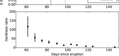
Figure 1: Swift XRT 0.3–10 keV count rate (upper panel), and hardness ratio (lower panel), defined here as the ratio hard/soft of the count rates in the 1–10 keV (hard) and 0.3–1 keV (soft) bands. The blue and red lines indicate the times of the Chandra and Suzaku observations, respectively.

In this paper, we focus on the optically thin X-ray emission observed with Swift, Chandra, and Suzaku from 61 to 155 days after the initial gamma-ray discovery, with the goal of probing the dynamics and mass of the ejecta. We reanalyze the Chandra spectrum from Day 85 presented in Peretz et al. (2016) in order to inform the analysis of the Suzaku and Swift observations. The data presented here were all obtained prior to the emergence of the white dwarf photosphere on Day 152. For a detailed study of the supersoft X-ray emission, see both Page et al. (2013) and Peretz et al. (2016).

2 Observations and Data Reduction

X-ray observations of V959 Mon were obtained with the Swift, Suzaku, and Chandra satellites. Here we provide details of the observations and the data reduction procedures for each satellite.

2.1 Swift

The Swift satellite began monitoring V959 Mon on 2012 August 19, shortly after the announcement of the optical discovery of the nova. Observations using the X-ray Telescope (XRT) were initially carried out at a roughly weekly cadence until the discovery of supersoft emission from the nova in the data obtained on 2012 Nov 28 (Day 162), at which point a daily observing campaign was initiated. Since the focus of this paper is the hard X-ray emission, we concentrate on the observations taken through 2012 Nov 11 (Day 146; see Table 1 for details of the observations).

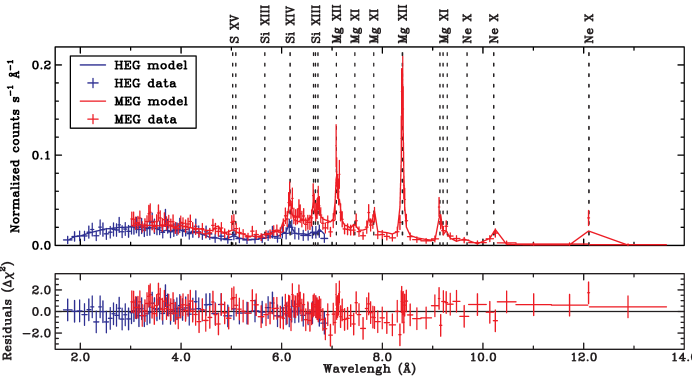
Figure 2: Chandra HETG data from Day 85, with best-fit model two temperature bvapec model shown as solid lines. The data are the summed 1st order HEG (blue) and MEG (red) spectra, grouped to have a minimum of 25 counts per bin. Residuals of the model fit (see Table 2 for parameters) are shown in the lower panel. The positions of strong emission lines, corrected for the best-fit blueshift of 770 km s^-1, are shown as dashed lines.

All of the XRT data included in this paper were obtained in photon counting (PC) mode, with exposure times ranging from 1880 to 5880 seconds. We created spectra for each observation using xselect v2.4b. Source photons were extracted from a circular region of radius 20 pixels ($\sim$47 arcsec) centered on the nova, while background events were extracted from a larger circular region located off the source. The source spectra were binned the to have a minimum of one count per bin. We used the xrtmkarf tool to create ancillary response files (ARFs) for each spectrum, correcting for dead columns and pixels using the exposure map included with the data from the archive. The source count rate in all observations was below 0.4 cts s^-1, so no additional corrections were made for pile-up. Finally, we downloaded the appropriate response matrix file (RMF) from the calibration database, in this case swxpc0to12s6_20110101v014.rmf. In our spectral fitting of Swift data, we binned the data to have a minimum of one count per bin, and used the C-statistic to determine best fit model parameters in the energy range 0.3–10 keV.

Table 1: Observation details

Date	Obs ID	$t_{\rm exp}$	Time since $t_{0}$
UT		(s)	(days)
Swift
2012 Aug 19	00032529001	5799	61.2
2012 Aug 26	00032529002	2033	68.4
2012 Sep 02	00032529003	5876	75.1
2012 Sep 09	00032529004	1704	82.0
2012 Sep 16	00032529005	2017	89.8
2012 Sep 23	00032529006	2001	96.4
2012 Sep 30	00032529007	1879	103.5
2012 Oct 06	00032529008	2023	109.2
2012 Oct 14	00032529009	1923	117.9
2012 Oct 21	00032529010	1924	124.5
2012 Nov 11	00032529011	1924	146.0
Chandra
2012 Sep 12	15495	24459	85
Suzaku
2012 Sep 25	907002010	46886	98

2.2 Chandra

In response to the discovery of bright X-ray emission from a nova detected as a gamma-ray source, a directors discretionary time (DDT) observation of V959 Mon was carried out with the Chandra satellite on 2012 Sept 12 (MJD 56182, Day 85 of the eruption; see Table 1). The total exposure time was 24.5 ks, and the observation was carried out using the high energy transmission grating (HETG) and the ACIS-S camera. The HETG instrument is comprised of two gratings, the High Energy Grating (HEG) and Medium Energy Grating (MEG), that in combination provide high spectral resolution over the wavelength range 1.5–30 Å (corresponding to photon energies of $\sim$0.4-8.2 keV). Preliminary results were reported by Ness et al. (2012), who noted the presence of blue-shifted emission lines and probably non-solar chemical abundances. A more detailed analysis of the Chandra spectrum was published previously by Peretz et al. (2016), as noted earlier.

We chose to reanalyze this Chandra spectrum in tandem with our exploration of the Suzaku and Swift datasets. We re-processed the data downloaded from the archive using the chandra_repro script and CIAO version 4.7. The processing script created new level 2 event files, and from that extracts the level two PHA files that contain the spectra. It also creates the response matrix (RMF) and ancillary response (ARF) files required for spectral modeling. Each spectrum was binned by a factor of two in channel space to increase signal to noise but maintain the energy resolution of the instrument. We fitted the four spectra ($\pm$1st orders for both HEG and MEG) independently, and used the C-statistic (Cash, 1979) to obtain best-fit model parameters and associated uncertainties. However, for plotting purposes, we co-added the +1 and $-$1 orders using the CIAO script (combine_grating_spectra) to increase the signal to noise in each spectral bin.

2.3 Suzaku

We requested a DDT observation of V959 Mon with the Suzaku satellite, which was approved and carried out on 2012 September 25 (MJD 56195, or Day 98 of the eruption; see Table 1). The total exposure time was 46.9 ks. No source was detected with the HXD instrument, so we focus on the data obtained with the X-ray Imaging Spectrometer (XIS) in the 0.3–10 keV energy range. All three functioning XIS units were operated in the full-window imaging mode. We extracted the source spectra from a circular region with a 3.5′ radius centered on V959 Mon, and background spectra from annular regions also centered on the source, with inner radius of 4′  and outer radius 6.5′. We created response files using the xisrmfgen and xisarfgen ftools, using the version 20120719 contamination files. Given the larger number of counts collected, we used the $\chi^{2}$ statistic to obtain best-fit model parameters and uncertainties.

3 X-ray evolution of V959 Mon as observed with Swift, Chandra, and Suzaku

The 0.3–10 keV count rate and hardness ratio for the Swift observation sequence are plotted in Figure 1, which reveals an X-ray evolution typical of novae weeks to months after the start of the eruption. The hardness ratio is defined here as the hard/soft count rate ratio above and below 1 keV. The X-ray emission becomes both brighter and softer with time through Day 100 or so, then levels off (Figure 1).

Although monitoring of V959 Mon with Swift provides a useful global view of the evolution of the X-ray emission, the short exposures and small number of collected photons means that some of the details of the X-ray emitting region, particularly those revealed by emission lines, are missed. The abundances of nova ejecta are known to be highly non-solar, with enhancements in CNO cycle elements from nuclear burning and in Ne if the underlying white dwarf is of the ONe subtype (see e.g. Helton et al., 2012, and references therein). Furthermore, the evolving nature of the eruption can lead to non-equilibrium ionization effects where emission line ratios have different values than those expected for plasmas in collisional ionization. To explore these details, we make use of the two deeper observations of V959 Mon that were obtained with the Chandra and Suzaku satellites.

The cross-calibration uncertainties among these observatories are small and well-understood, thanks to the efforts of the International Astrophysical Consortium for High Energy Calibration (IACHEC). Cross-calibration issues can generally be ignored in combined analyses of data from these unless the observations are all well-exposed and have small statistical errors so that differences become evident, which is not the case here. We therefore infer that any disagreements in the fit results are due to statistical limitations of the data, source variability, or our limited understanding of the underlying physics, as reflected in our choice of spectral models.

In this section, we present our spectral analysis of the data obtained with all three satellites. We first revisit the Chandra spectrum presented in Peretz et al. We then use the insights from the Chandra modeling to analyze the Suzaku spectrum obtained on Day 98. Finally, we analyze the set of Swift spectra using the abundances found from the analysis of the two deep spectra. Given the presence of emission lines in the Chandra and Suzaku spectra, we modeled all spectra in xspec v12.8.0m using the APEC suite of thermal, collisional plasma models. We used the tbabs model for foreground absorption assuming the photoionization cross-section values of Verner et al. (1996). In addition, we initially assume the the abundances of Wilms et al. (2000) for the absorber. This assumption is appropriate for the interstellar medium, but as we show below, we detect significant absorption from parts of the nova ejecta. We discuss the consequence of an alternative assumption regarding the absorber composition, perhaps more appropriate for this situation, in Section 4.3.

3.1 Revisiting the Day 85 Chandra spectrum

The Chandra spectrum obtained on Day 85 is dominated by emission lines of hydrogen- and helium-like Si and Mg, and hydrogen-like Ne. Peretz et al. (2016) presented an analysis of this Chandra spectrum and found an acceptable fit to the data with a two-temperature collisional ionization equilibrium (CIE) plasma model with highly enhanced abundances of metals, including Ne, Mg and Al. The emission lines were blueshifted by $850_{-145}^{+75}$ km s^-1 in the low temperature component, but not in the hotter plasma (which were frozen to zero). Finally, both plasmas showed broadened lines, with a FWHM velocity of 676${}_{-70}^{+80}$ km s^-1; this value was assumed to be the same in both temperature components.

We modeled the Chandra data utilizing the entire wavelength range of the HEG (1.5–15 Å; 0.83–8.3 keV), and a subsection of the MEG range (2–20 Å; 0.62–6.2 keV) as there is very little signal at longer wavelengths. In our fit, we used the same model (tbabs*(bvapec+bvapec)) as Peretz et al. (2016), with a few key differences. First, we assume abundances for He, C, N and O determined from optical spectroscopy of V959 Mon by Tarasova (2014), and keep these values fixed. Second, we allow the line broadening of the two components to vary freely. Finally, we assume a single velocity shift for the two components, but compare our results with those of Peretz et al. below.

In Figure 2, we show the combined 1st order HEG and MEG spectra with our best-fit model and residuals. The resulting model parameters, shown in Table 2, are broadly compatible with the findings of Peretz et al. (2016). The two plasma temperatures are 3.7 and 0.64 keV, which are slightly lower values than those presented by Peretz et al. (4.5 and 0.8 keV, respectively). The absorbing column towards the X-ray emitting region is (3.2 $\pm$ 0.2) $\times$ 10²² cm^-2. The abundances of Ne, Mg, Al, Si and S are all strongly enhanced relative to reference values (see Table 2 for values). The abundance of Fe is poorly constrained by the spectra, which is not surprising given the lack of strong Fe lines in the data, and we find only an upper limit on Fe/Fe_⊙ of $<$1.5 at the 90% confidence level. We find line broadening of 1370 and 510 km s^-1 for the 3.7 and 0.6 keV plasmas, respectively. Finally, our best-fit model indicates a blueshift in the line positions of 771${}^{+71}_{-66}$ km s^-1, which is within the uncertainty range found by Peretz et al. (2016) for the lower temperature component. We note that the fit statistic found when the blueshift of the 3.7 keV component is fixed to zero (as in Peretz et al.) is not significantly different to our best-fit, single velocity shift model, and none of the other model parameters change within the uncertainties. We take this to mean that there is a degeneracy in the line centroid and the line width, when fitting two-component spectral models to the Chandra grating data of this nova. The data tell us that the two components have different kinematic signatures, but we cannot tell whether the difference is in the velocity shift or in line width.

Table 2: Best-Fit Model Parameters for Chandra and Suzaku Spectra. Model is of form tbabs*(bvapec+bvapec) with redshift and abundance set equal for both bvapec components.

	Chandra	Suzaku
NH (1022 cm-2)	3.2 $\pm$ 0.2	1.44${}^{+0.06}_{-0.05}$
blueshift (km s-1)	771${}^{+71}_{-66}$	771a
kT1 (keV)	3.7${}^{+0.5}_{-0.4}$	3.9 $\pm$ 0.1
norm${}_{1}^{b}$	0.005 $\pm$ 0.002	0.009 $\pm$ 0.0003
velocity width (km s-1)	1362${}^{+315}_{-259}$	1362a
kT2 (keV)	0.64${}^{+0.10}_{-0.05}$	0.311${}_{-0.008}^{+0.009}$
norm${}_{2}^{b}$	0.0010${}_{-0.0006}^{+0.0007}$	0.0024 $\pm$ 0.0003
velocity width (km s-1)	515${}^{+87}_{-77}$	515a
He/He⊙	1.5	1.5
C/C⊙	1	1
N/N⊙	33	33
O/O⊙	9.2	9.2
Ne/Ne⊙	207${}_{-93}^{+323}$	19${}^{+3}_{-2}$
Mg/Mg⊙	55${}_{-21}^{+73}$	20 $\pm$ 2
Al/Al⊙	51${}^{-23}_{+70}$	25${}^{+7}_{-6}$
Si/Si⊙	6${}^{+8}_{-3}$	2.3 $\pm$ 0.5
S/S⊙	4${}^{+5}_{-2}$	1.9$\pm$ 0.4
Fe/Fe⊙	$<$1.5	0.17$\pm$ 0.05
XIS 1 normalization	$\ldots$	1.0
XIS 0 normalization	$\ldots$	1.00 $\pm$ 0.01
XIS 3 normalization	$\ldots$	1.01 $\pm$ 0.01
$F_{0.3-10}$ (10-11 erg s-1cm-2)c	1.70${}^{+0.04}_{-0.67}$	1.61 $\pm$ 0.02
$L_{0.3-10}$ (1034 erg s-1)	1.4 $\pm$ 0.2	1.07 $\pm$ 0.02
C-stat (Chandra) or $\chi^{2}$ (Suzaku)	5799	3919
D.O.F	9182	2684
aVelocity shift fixed to Chandra value.
bnorm = $\frac{10^{-14}}{4\pi D^{2}}\int n_{e}n_{i}dV$
cWe used the energies command in xspec to extend the
energy coverage of the HETG response down to 0.3 keV.
All quoted uncertainties are 90% confidence intervals.

The lower temperature plasma component in the model appears to be necessary to explain the ratios of H- to He-like lines in the spectrum (particularly for Mg) which cannot be reproduced by a single temperature model. Non-equilibrium ionization models can in principle also account for H-like to He-like line ratios that depart from the values expected in CIE models (see the case of V407 Cyg; Nelson et al. 2012). However, the density we infer for the X-ray emission region makes this alternative interpretation unlikely, as we discuss in subsection 4.4.

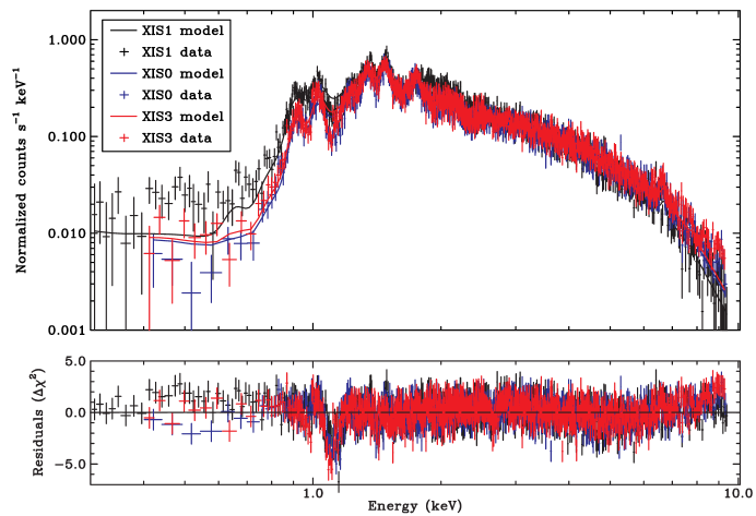
Figure 3: Suzaku XIS data from Day 98, with best-fit model shown as solid lines. Residuals of the model fit as shown in the lower panel. The parameters of this model are shown in Table 2.

3.2 Suzaku view on Day 98

To model the Suzaku spectra, we used the 0.3–10 keV range for the XIS1 instrument, and 0.4–10 keV for XIS0 and XIS3. Our starting point was the best-fit model found for the Chandra data. Since the line-broadening derived from the model fits to the HETG spectra is less than the instrumental spectral resolution of the Suzaku XIS CCDs, we fixed the line broadening to those found for the Chandra spectra when fitting the XIS data. We also fixed the blueshift value of the models to $v$ = 771 km s^-1, the best-fit value found in modeling the Chandra data. The resulting best-fit parameters are shown in Table 2, and the data, model and residuals are shown in Figure 3.

The temperature of the hotter component in the two-temperature CIE model (column 3 in Table 2) is 3.9 $\pm$ 0.1 keV, in agreement with the value found for the Chandra spectrum within the uncertainties. In contrast, a lower temperature of 0.32 $\pm$ 0.01 keV is found for the second component. The normalizations, and hence emission measures, of both temperature components are slightly higher than those found in the best-fit Chandra model. Given that the overall flux is slightly lower, this is most likely an effect of the lower best-fit abundances in this model, which are lower than in the Chandra model, and have much smaller uncertainties. This difference is most notable for neon, where we find Ne/Ne_⊙ = 19${}^{+3}_{-2}$, and for iron, where we find Fe/Fe_⊙ = 0.17 $\pm$ 0.05. Finally, the absorbing column attenuating the X-ray emission is also lower than in the Chandra fit, with N_H = 1.4 $\times$ 10²² cm^-2. This results in a lower unabsorbed flux and inferred luminosity.

The fit of this model is by no means perfect; the reduced $\chi^{2}$ value is 1.46, and clear residuals are seen in the fit to the data. The best-fit model underestimates the Suzaku data at energies $>$8 keV. We note that the V959 Mon region of the X-ray sky is somewhat crowded (Evans et al., 2014) and it is possible that the excess is due to a highly absorbed source within the 210" radius extraction region. There is also a significant negative residual ($\sim$6–7$\sigma$) at 1–1.1 keV. There are several lines of Fe and a line of helium-like Ne that is strong in plasmas with kT of around 0.3 keV. Given that the best-fit Fe abundance is very low, the discrepancy is likely to be due to the Ne line. Finally, the apparent detection of signal below 0.7 keV is entirely consistent with the low-energy tail in the CCD response to higher energy photons, due to incomplete collection of charges. This is a feature commonly seen in heavily absorbed sources, and is known to be less well calibrated than the main part of the detector response. We nevertheless show the data down to 0.3 (for XIS1)/0.4 (for XIS0 and XIS3) keV, to demonstrate the absence of photons from V959 Mon at these energies, such as the supersoft component or strong low-energy emission lines.

3.3 X-ray evolution observed with Swift is driven by evolving absorption

We further investigated the X-ray evolution of V959 Mon, already seen in the plot of 0.3–10 keV count rate and hardness ratio (Figure 1), by fitting models informed by our analysis of Chandra and Suzaku spectra to the XRT spectra. We first attempted to fit a two-temperature plasma model of the same form as those in Table 2 to each XRT spectrum, fixing the elemental abundances to those found for Chandra or Suzaku. However, these model fits were unstable and parameter uncertainties could not be derived. Given that the higher temperature component dominates the flux of the best-fit models for both the Chandra and Suzaku spectra, we decided to model the X-ray emission in the XRT spectra using single temperature model (tbabs*bvapec), assuming the best-fit Suzaku abundances listed in Table 2. The modeling results are shown in Table 3, and plotted in Figure 4. We note that very similar values are found when assuming the Chandra abundance set. In addition to the Swift results, Figure 4 includes the best-fit parameters for the hotter component from the Chandra and Suzaku observations (see subsection 3.4 for a discussion of similarity and differences in the derived parameter values).

The most striking aspect of the spectral evolution is the large decrease in the column density of the absorber, from 4.8 $\times$ 10²² to 2.4 $\times$ 10²¹ cm^-2 over the course of the observations. This change in the absorbing column appears to be the primary reason for the increase in flux over the first 6 weeks of the monitoring campaign. The physical properties of the plasma component appear to be more stable over the same time period; the temperature is approximately constant (roughly 4 keV) between Days 61 and 125, and only begins to drop significantly in the observation on Day 146, to 2.6 keV. While there is indication of a higher plasma temperature between Days 80 and 100, the uncertainties on these temperature estimates are large, and the values derived from the Chandra and Suzaku data during the same time period are consistent with the 4 keV plasma being continuously present over this time period. The emission measure (derived from the normalization of the vapec model and assuming a distance to the nova of 1.4 kpc) shows some variability over the same time period. Between Days 61 and 125, if there is a systematic decline in the emission measure, it is masked by the scatter in our measurements. The emission measure on Day 146 is clearly lower.

3.4 Comparing the Swift, Chandra, and Suzaku results

The abundances found for the Chandra and Suzaku data sets, taken at similar times, are quite different within the framework of the same 2-temperature plasma models and fixing the He, C, N, and O abundances to values derived from optical observations. The largest discrepancy in the estimate of the Neon abundance, which is a factor of 10 larger for the Chandra best-fit model than for Suzaku. The other free-to-vary-elements differ by a factor of a few between the two models, with the Chandra model having the larger abundances. A high neon abundance (Ne/Ne_⊙ = 95) was also reported by Tarasova (2014) from optical data, although they also reported a higher iron abundance (Fe/Fe_⊙ = 1.5) which is only consistent with our estimate from the Chandra data at the 90% upper limit. The Fe abundance is even lower in the Suzaku data. We discuss potential causes for discrepant abundance measurements in subsection 4.6. We note, however, that the absolute abundances are estimated from X-ray data assuming hydrogen ions dominate the Bremsstrahlung continuum. Since all ions contribute to the Bremsstrahlung continuum, and nova ejecta have non-solar abundances, this leads to considerable systematic uncertainties, particularly due to the non-solar abundance of helium, which X-ray data cannot constrain. Moreover, even the determination of the relative abundances of medium-Z elements can be challenging if multiple plasma temperatures are present. What we can conclude for certain is that the X-ray emitting gas is enhanced in elements typically observed in nova ejecta.

The agreement between the best-fit parameters obtained for the Chandra and Suzaku spectra and those found for the Swift observations taken most closely in time is good for some parameters, and less so for others. The Suzaku temperature estimate agrees closely with that found for the Swift observations taken immediately before and after, with most values falling around 3–4 keV. The Chandra value is slightly lower than its neighboring XRT values, although we note the large uncertainties in these parameters, and the closer agreement between Chandra and deeper Swift observations (i.e., those with smaller error bars in Figure 4). The N_H value found in the Chandra observation is much higher than the Swift observations taken immediately before and after. The agreement between the Suzaku and Swift N_H values is better, but still not perfect. Unabsorbed fluxes, and therefore luminosities are higher in the deep spectra, but this is not surprising given the different N_H values found and the fact that these models include a lower kT component which adds additional flux at lower energies.

The high N_H value found for the Chandra spectrum was also noted by Peretz et al. (2016). HETG does not have sufficient sensitivity to detect and characterize the continuum longward of 10 Å, while it does detect Ne lines in this spectral region. The Chandra spectral fits (both our own and that of Peretz et al. 2016) found solutions with extremely high Ne abundances, hence very high intrinsic fluxes for the Ne lines. The high N_H value is necessary to bring down the predicted line fluxes to the observed levels. Both Suzaku and Swift have higher effective areas and are more sensitive to the continuum in this spectral region. The disagreement between Chandra and the other two instruments may indicate that our chosen model does not describe the emission line ratios accurately. In terms of N_H, we proceed assuming that the values derived from the continuum using Swift and Suzaku data are more reliable, which also implies that the lower Ne abundance determined with Suzaku is closer to the truth.

Table 3: Swift spectral fitting results using best-fit Suzaku abundances

Time	Obs ID	rate	NH	kT	normalization1	$F_{0.3-10~{}{\rm keV}}$	$L_{0.3-10~{}{\rm keV}}$
(Day)		(cts s-1)	(1022 cm-2)	(keV)	(10-3)	(10-11 erg s-1cm-2)	(1033 erg s-1)
61.2	00032529001	0.13	4.8 $\pm$ 0.4	3.6${}^{+0.7}_{-0.5}$	0.010 $\pm$ 0.001	1.10${}^{+0.04}_{-0.08}$	6.6 $\pm$ 0.3
68.4	00032529002	0.17	2.4 $\pm$ 0.4	10.3${}^{+10.4}_{-3.9}$	0.007${}^{+0.0007}_{-0.0005}$	1.42${}^{+0.07}_{-0.25}$	5.1 $\pm$ 0.4
75.1	00032529003	0.17	2.3 $\pm$ 0.2	4.3${}^{+0.7}_{-0.4}$	0.009 $\pm$ 0.0005	1.32${}^{+0.09}_{-0.07}$	5.8 $\pm$ 0.3
82.0	00032529004	0.24	1.7 $\pm$ 0.3	6.9${}^{+4.7}_{-1.6}$	0.008 $\pm$ 0.0008	1.61${}^{+0.24}_{-0.21}$	5.8${}^{+0.4}_{-0.3}$
89.8	00032529005	0.23	1.2 $\pm$ 0.2	6.2${}^{+2.0}_{-1.3}$	0.007 $\pm$ 0.0005	1.38${}^{+0.12}_{-0.13}$	4.7 $\pm$ 0.3
96.4	00032529006	0.27	1.0 $\pm$ 0.1	4.6${}^{+0.9}_{-0.7}$	0.008 $\pm$ 0.0005	1.44${}^{+0.11}_{-0.10}$	5.1 $\pm$ 0.3
103.5	00032529007	0.31	1.0 $\pm$ 0.1	4.2${}^{+0.9}_{-0.5}$	0.009 $\pm$ 0.0005	1.63${}^{+0.12}_{-0.10}$	5.8${}^{+0.3}_{-0.4}$
109.2	00032529008	0.34	1.0 $\pm$ 0.1	5.0${}^{+1.0}_{-0.7}$	0.009 $\pm$ 0.0006	1.77 $\pm$ 0.12	6.1 $\pm$ 0.3
117.9	00032529009	0.31	0.6 $\pm$ 0.1	3.8 $\pm$ 0.5	0.007 $\pm$ 0.0005	1.32 $\pm$ 0.08	4.4${}^{+0.2}_{-0.3}$
124.5	00032529010	0.31	0.5 $\pm$ 0.1	4.1${}^{+0.8}_{-0.5}$	0.006 $\pm$ 0.0004	1.37 $\pm$ 0.08	4.3 $\pm$ 0.2
146.0	00032529011	0.26	0.2 $\pm$ 0.1	2.5${}^{+0.5}_{-0.4}$	0.003 $\pm$ 0.0003	0.80 $\pm$ 0.06	2.2 $\pm$ 0.2
1The normalization of the bvapec model is defined as 10-14/4$\pi$d2 $\int n_{e}n_{H}dV$, where $d$ is the distance
to the source in cm, and $n_{e}$ and $n_{H}$ are the densities of elections and hydrogen, respectively, in the
shocked plasma. All quoted uncertainties are 1$\sigma$.

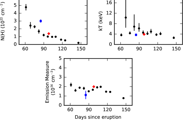
Figure 4: Parameters for the hotter X-ray component derived from spectral fits to Swift (black), Chandra (blue) and Suzaku (red) observations taken between 60 and 150 days after the June discovery of the nova with Fermi. Upper left: The observed (absorbed) X-ray flux of the source, measured in the 0.3–10 keV energy range. Upper right The intrinsic luminosity of the source, determined by correcting for absorption, for an assumed distance of 1.4 kpc. Middle left Evolution of the absorbing column density, assuming the ISM abundances. Middle right: Evolution of the plasma temperature. Lower center The X-ray emission measure, derived from the normalization of the apec model.

3.5 Constraints on the density of the nova ejecta

Peretz et al. (2016) claim that the X-ray emitting region observed with Chandra in V959 Mon must have very high density of at least 6 $\times$10¹⁰ cm^-3 (1$\sigma$; with a 3$\sigma$ lower limit of order 10⁹ cm^-3). The authors derive this value from their estimates of the Mg XI line fluxes via the He-like density diagnostic discussed in Porquet et al. (2001), under the assumption that the X-ray emitting region is illuminated very weakly by radiation from the central source. The ratio $R=f/i$, where $i$ and $f$ are the intercombination (the middle component of the triplet) and forbidden (longest wavelength component) emission lines of a He-like ion, is sensitive to density under certain physical conditions. Peretz et al. (2016) find a value of $R$ = 1.40 $\pm$ 0.52 (1-$\sigma$ error), implying the above density limit, and deduce that the X-ray emitting material must be highly clumped in order to explain the observed emission measure.

Given the limited statistical quality of the HETG spectra, it is quite likely that there is an additional uncertainty on the $R$ measurement that Peretz et al. (2016) did not account for, e.g., that due to the line widths and shifts. To help assess the range of uncertainties on $R$, we carried out our own fits to the Mg XI triplet. We focus only on the MEG spectrum, binned by a factor of 2 in channel space, since there is very little signal in the HEG spectrum at these wavelengths. We modeled the region of the spectrum between 8.7 and 9.45Å as the sum of a power law continuum with spectral index $-$2.5 and three Gaussian lines to represent the He-like triplet. The rest-frame energy of all three lines was fixed to their values as reported by the ATOMDB website, and all three components were tied to have the same blueshift, which varied freely in the fit. Finally, the line width was constrained to the 90% confidence interval found in our global model, or 515${}^{+87}_{-77}$ km s^-1. In order to estimate the uncertainty on the ratio $R$, we made use of the Markov Chain Monte Carlo functionality in xspec, producing 20,000 realizations of the model compared to the data and using this to determine the distribution of $R$ that is compatible with the data.

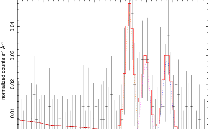
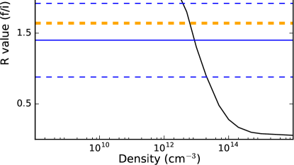
Figure 5: Upper panel: Best-fit three Gaussian plus power-law model to the Mg IX triplet region of the MEG data. The lines (with laboratory wavelengths of 9.17, 9.23, and 9.31 Å for the resonant, intercombination, and forbidden components, respectively) are blueshifted by 1100 km s^-1. Lower panel: Density diagnostic data from Porquet et al. (2001), assuming photoionization is negligible (T_rad=0.0, W=0.01). The derived $R$-value and 1-$\sigma$ uncertainties from Peretz et al. (2016) are shown in blue as solid and dashed lines, respectively. The 1- and 2-$\sigma$ upper limits found by us are shown in orange.

The best-fit model is shown in the upper panel of Figure 5. The best-fit blueshift is larger than the value found for the global model, with $v$ = 1100 $\pm$ 200 km s^-1. We find only weak upper limits to $R=f/i$. The 1- and 2-$\sigma$ upper limits are shown as orange dashed and dash-dotted lines in the lower panel of Figure 5. At the 2-$\sigma$ level, we find that the observed lines are un-constraining as a density diagnostic. Given the uncertainties introduced by the presence of an unquantified radiation field, density variations in the emitting regions, and the fact that we are approximating lines that are most likely asymmetric with Gaussians, the constraints on $R$ are probably even weaker than the ones we find here; ultimately, we are fundamentally limited by the low S/N of the data. Even so, we comment on the possible high density of the X-ray emitting region in subsection 4.4, in light of our other findings.

4 Details of the mass ejection process in V959 Mon

As we discuss in the introduction, Chomiuk et al. (2014a) explained the observed evolution of the resolved radio images of V959 Mon obtained with the VLA with a two phase mass ejection, in which slower material expelled preferentially in the orbital plane at early times is followed by a period of fast mass loss. This fast outflow leaves the system preferentially in the polar direction, which is the path of least resistance away from the dense equatorial material. This dense equatorial waist (or “torus”) plus bipolar lobe geometry was confirmed by Hubble Space Telescope (HST) narrow-band imaging and Space Telescope Imaging Spectrograph (STIS) spectroscopy (Sokoloski et al., 2017). Synchrotron blobs were observed at the interaction region between these two systems of ejecta, suggesting the presence of relativistic material accelerated in shocks at the contact surface.

We propose that the same geometry can explain the evolution we see in the X-ray data. The shock interaction of the two systems of ejecta that produces synchrotron emission also leads to the emission of X-rays from the forward and reverse shock regions. Schematically, the nova ejecta will exist in the form of the unshocked wind, the reverse shock front, shocked wind matter, the contact discontinuity, the shocked torus matter, the forward shock front, and the unshocked torus matter, from the central binary out to interstellar space. We assume no mixing between the torus matter and fast wind on the time scale of our observations. This outermost layer, the unshocked warm matter in the edge-on torus then absorbs this X-ray emission, producing the visible spectral signature of high N_H material we see in the Swift data. As the equatorial torus expands away from the central binary, the column density towards the X-ray emission drops. In the rest of this paper, we will distinguish between the N_H value of the interstellar medium (N_H,ISM) and that of the unshocked nova ejecta (N_H,int; for “internal” column). We continue to use the symbol N_H for the observed column, which is the sum of N_H,ISM and N_H,int.

The X-ray observations analyzed here provide a wealth of information regarding the shock interaction between these two systems of outflows. However, the situation is complex with many unknowns, including the evolution of mass loss rate in the fast flow, so that we cannot arrive at a unique model. We therefore focus on aspects that can be solved with existing data with a minimum set of assumptions. In the following, we argue that the long-lived nature of the hot ($\sim$4 keV) component favours its origin in the reverse shock driven into the fast outflow. We then discuss the evolution of the absorbing column, and conclude that the slow torus was ejected weeks after the thermo-nuclear runaway. Furthermore, we estimate the total mass of the slow ejecta, and also its average density at the inner edge. We then use the observed X-ray luminosity to constrain the mass loss rate of the fast outflow, and its density. We further consider the kinematics and the densities of the X-ray emitting regions. We then briefly touch on the issue of abundances. Finally, we discuss the implications of our findings on the gamma-ray emission from V959 Mon in particular, and novae in general.

4.1 The Reverse Shock as the Likely Origin of X-rays

In principle, the observed X-rays can be dominated by the forward shock driven into the torus or the reverse shock driven into the bipolar wind, or the X-rays may be due to a combination of both. Here we propose that the predominant source of observed X-ray emission was the reverse shock driven into the fast outflow, based on a two stage argument. First, we argue that the long-lived X-ray emission likely requires a long-lasting shock interaction. We then argue that the slow torus is not physically extensive enough to allow a forward shock to persist long enough to explain the evolution of the X-rays. The reverse shock, on the other hand, can exist as long as the fast wind persisted.

There was a long plateau phase during which we do not observe an obvious downward trend in kT or luminosity, from the start of our Swift observations around Day 60 to about Day 120. The plateau phase could have started earlier in reality, but we simply do not have any X-ray data on V959 Mon before Day 61. If the shock had a high density as Peretz et al. (2016) inferred, the cooling time is a fraction of a day (see subsection 4.4), so such individual clumps would radiatively cool and cannot persist at the same temperature for over 60 days. If the true density of the shock was much lower, as is allowed by our analysis, then the radiative cooling time can be longer. However, the radius of the nova ejecta ($r$) will have expanded by a factor of 2 (for an instantaneous ejection at the time of the thermonuclear runaway) or more (for a delayed ejection; see subsection 4.2) from Day 60 to 120; we expect this to lead to significant adiabatic cooling. A continuing supply of freshly shocked material, heat, and pressure is essential to maintain a roughly constant kT and a roughly constant luminosity.

The near constancy of kT during the plateau phase suggests that the shock velocity (the velocity of the shock front relative to the unshocked matter) was also nearly constant during this period. The Rankine-Hugenot conditions for a strong shock relates the maximum shocked plasma temperature to the shock velocity as

$$v_{s}=\sqrt{{16\ {\rm kT}_{\rm br}}\over{3\ \mu\,m_{H}}}=1000\left({{\rm kT}\over{1.2{\rm keV}}}\right)^{1/2}\left({\mu\over 0.62}\right)^{-1/2}{\rm km}\,{\rm s}^{-1}$$

where $\mu$ is the mean molecular weight of the gas and $m_{H}$ is the mass of a hydrogen atom. For solar abundances, $\mu\sim 0.62$, which we use here as the fiducial value, while the overabundance of metals suggests a somewhat higher $\mu$, perhaps as high as 1.0. The above formula incorporates the fact that the post-shock plasma is moving at 1/4$v_{s}$. During the plateau phase (Day 60–120) when the observed temperature remained kT $\sim$ 4.0 keV, the shock velocity was 1820 km s^-1 in the solar abundance case, and as low as $\sim$1300 km s^-1 if $\mu$ was close to 1.0. We must add the velocity of the unshocked torus to estimate the velocity of the shock front relative to the central binary, which is greater than 2000 km s^-1. Thus, if the X-rays originated in the forward shock, the shock front would have traveled about 9$\times 10^{9}$ (7$\times 10^{9}$) km or $\sim$60 ($\sim$45) AU relative to the torus matter during the $\sim$60 day plateau phase assuming $\mu\sim 0.62$ ($\mu\sim 1.0$).

This is larger than to the expected physical size of the torus. If the torus was build up from $t_{0}$ by a constant velocity flow, that velocity would have to have been equal to or greater than the shock velocity to have build up a 60 AU thick torus by Day 60, whereas a variety of clues suggests the predominant velocity of the slow torus was less than 1000 km s^-1. In this case, the outward movement of the torus during the plateau phase is irrelevant. If, on the other hand, the torus has a range of velocities (such as the Hubble flow type structure we adopt below), this would allow the range of radius that the torus occupies to grow with time. However, in this case, we expect the shock velocity to decrease as the shock front catches up with faster and faster parts of the torus. Therefore, the constant shock temperature is hard to explain. In either case, the forward shock interpretation seems hard to sustain.

It is common for optical spectra of novae near maximum to show variable outflow velocities, or of appearance and disappearance of multiple outflow components (see, e.g., Aydi et al. 2020). This might bring to mind the possibility of multiple shocks. However, the passage of a single shock front would have left the torus in an altered dynamical state, and it seems problematic to postulate multiple shocks through the torus with an identical shock temperature. Moreover, optical spectra of V959 Mon throughout the plateau phase show emission line profiles that changed little (Ribeiro et al., 2013; Shore et al., 2013).

The reverse shock driven into the fast, inner flow, on the other hand, could have moved outward or inward relative to the central binary during the plateau phase, depending on the wind velocity. In either case, it can maintain a constant shock temperature, as long as the inner flow with a velocity greater than the shock velocity persisted during the plateau phase. Thus, we adopt the reverse shock as the likely origin of the predominant (kT$\sim$4 keV) component of X-ray emission. In this case, the forward shock may well be the site of the lower temperature component identified with Chandra and Suzaku. The lower shock velocity allows the forward shock to persist longer, and the Hubble flow picture even provides a potential explanation for the apparent decrease of the temperature of the soft component.

4.2 The N_H evolution is not consistent with a shell expanding since Day 0

The column density of the material absorbing the X-ray emission from an internal shock in a nova is expected to decrease with time as the slower ejecta expand and the density drops (Mukai & Ishida, 2001). The X-ray monitoring of V959 Mon presented here provides one of the clearest examples of this behavior. For a single, thin, shell, this drop is proportional to $r^{-2}$. However, more realistically, both the maximum absorption and the rate at which the column density drops depend on the mass and velocity structure of the ejected shell, and so the observed N_H,int values and evolution with time can be used to place some basic constraints on the properties of the ejected shell. In order to do this, we modeled the N_H,int evolution observed with Swift using a simple model of a spherically symmetric shell that expands at a constant rate with time.

We assume that the shell has an $r^{-2}$ density profile between the inner radius $r_{\rm in}$ and the outer radius $r_{\rm out}$. We further assume that the velocity of the expanding shell is linearly proportional to radius, between the smallest value $v_{\rm in}$ at $r_{\rm in}$ and the largest value $v_{\rm out}$ at $r_{\rm out}$, and the time since ejection can be used to translate between the radius and the velocity. This is the same “Hubble flow” structure commonly used to model radio emission from novae (see Seaquist & Palimaka, 1977, for details). A single normalization factor related to the total ejecta mass is then required to estimate the integrated absorbing column through such a shell, for a given set of $v_{\rm in}$ and $v_{\rm out}$. As the shell expands, the intrinsic column density will drop with time, and the observed N_H will asymptotically approach N_H,ISM.

A range of estimates of N_H,ISM towards V959 Mon exist in the literature. Shore et al. (2013) favour an E(B$-$V) of 0.8 mag, implying an N_H,ISM value of 5.5 $\times$ 10²¹ cm^-2 using the E(B$-$V) to N_H conversion of Güver & Özel (2009). Munari et al. (2013) argue for a smaller E(B$-$V) of 0.38 $\pm$ 0.01, implying N_H,ISM of just 2.5 $\times$ 10²¹ cm^-2. In the following work, we examined three values of N_H,ISM; 2.5, 3.5, and 5.0 $\times$ 10²¹ cm^-2.

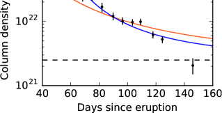
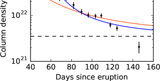
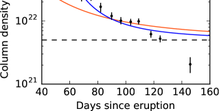
Figure 6: N_H evolution determined from Swift spectra, compared with models of N_H,int evolution for nova shells with a $r^{-2}$ density profile and inner (outer) velocities of 770 (2400) km s^-1. We assume three values for the interstellar column density (N_H,ISM; shown as dashed horizontal lines). The solid red lines show the best-fit models ejected at the time of the Fermi detection, and have $\chi^{2}$/DOF values of 11.4, 14.1 and 18.8, respectively. The blue lines are the best-fits for a delayed expansion model, which have $\chi^{2}$/DOF values of 3.2, 4.5 and 7.5, respectively.

In Figure 6, we show comparisons of the data with our simple model of N_H,int evolution for an $r^{-2}$ density profile shell, assuming the three adopted values of N_H,ISM. Using the lmfit package in python (Newville et al., 2014), we fit the N_H values derived from spectral fitting of the Swift XRT spectra, with the abundances found for the bvapec model fit to the Suzaku data, with our N_H,int evolution model. We excluded the N_H value obtained on Day 146 (see below). Since the ejected mass and expansion velocity are degenerate, we initially fixed $v_{min}$ to 770 km s^-1 (assuming that the blueshift of the X-ray emission is indicative of the the inner velocity of the dense shell), and $v_{max}$ to the maximum velocity implied by the bipolar model of Ribeiro et al. (2013), 2400 km s^-1. We then fit for the ejected mass. The best-fit N_H found on Day 146 lies well below the model in all cases. This value is also lower than the N_H reported for later Swift observations during the supersoft phase of the nova evolution. We speculate that the N_H derived for this spectrum is anomalous due to the earliest presence of the photospheric emission, even though it is not clearly recognizable as such, making the spectrum flatter and the implied N_H smaller.

Regardless of the assumed N_H,ISM value, shell models ejected at t₀ (i.e. the time of the Fermi detection) do not give a good fit to the best-fit column density values. These models, shown as the red lines in Figure 6, decline at a slower rate than the data values, and have difficulty accounting for the high N_H observed before Day 80. Therefore, we also fit models that leave the start date of the expansion of the ejecta (hereafter $t_{e}$) a free parameter (fixing the N_H,int to a high value before that time). The delayed ejection models result in a much better fits to the data at early times than the t₀ ejection models, for all assumed values of N_H,ISM. The derived delay times get later as the assumed N_H,ISM increases in value, from 38 days for N_H,ISM = 2.5 $\times$ 10²¹ cm^-2 to 45 days for N_H,ISM = 5 $\times$ 10²¹ cm^-2. For each assumed value of interstellar absorption, N_H,ISM, the ejection time is constrained by the decline rate of the observed N_H values (as long as the shell expands at constant velocity), and so is independent of the assumed inner and outer velocities of the shell. The overall best-fit to the data is obtained for N_H,ISM = 2.5 $\times$ 10²¹ cm^-2.

Absorption of X-rays with photon energies in the $\sim$1 to several keV range is largely due to K shell electrons of medium-Z elements, such as Oxygen. If, during the course of Swift XRT monitoring, an increasing fraction of the slow torus becomes shocked, and therefore become ionized, then the measured N_H values would decline faster than the above analysis would suggest. This effect is unlikely to explain the discrepancy between the measurements and the prompt ($t_{e}$=$t_{0}$) ejection model: if this was the reason for the faster-than-expected decline of N_H,int before Day 82, we expect the decline to continue to be faster than the unshocked prompt ejection model after Day 82, which is not what we observe. On the other hand, it is possible that the ionization of the slow torus is in part responsible for the poor agreement between the data and the models (prompt or delayed) at late times, say after Day 110.

We note that Linford et al. (2015) also found evidence for a delay in spatial expansion of the radio-emitting nova shell of V959 Mon in VLA images obtained during Days 126–199. During these times, the VLA images are elongated in the east-west direction due to the spatial extension of the fast outflow. The angular diameters in the north-south direction of both the eastern and western lobes are seen to expand from 0.06 to 0.11 arcsec. The measurements are consistent with expansion at constant velocity that started at Day 25 $\pm$ 10 (see Figure 8 of Linford et al. 2015). Since this refers to the fast outflow, while the delay inferred from the X-ray N_H evolution is that of the slow torus, they are not direct corroborations of each other. Nevertheless, it seems encouraging that independent observations of two distinct components of outflow in V959 Mon both indicate delayed ejection, perhaps suggesting a common origin for the delay.

Recently, Sokolovsky et al. (2020) also inferred a delayed ejection of the torus in V906 Car (=ASASSN-18fv), by analyzing the N_H evolution of its X-ray emission. Moreover, a similar delayed ejection scenario was proposed to explain the concurrent radio and X-ray evolution of T Pyx during its 2011 eruption (Nelson et al., 2014; Chomiuk et al., 2014b). In that system, radio emission did not start rising until $\sim$60 days after eruption, based on radio flux density evolution and the late onset of hard X-ray emission. Stalled expansion may be common in novae, and implies a phase where common envelope physics can influence mass ejection and angular momentum loss from the system.

Our working model, then, is that the thermonuclear runaway can leave some fraction of the accreted matter in an extended, quasi-static configuration, having a red giant-like dimension. Optical spectroscopy measures the expansion velocity of the part of the envelope that is promptly ejected to infinity, but we do not have a direct velocity measurement of the matter responsible for the optical continuum. We postulate that the continuum source is the quasi-static, marginally-bound envelope, to borrow the terminology of Pejcha et al. (2016). Such an extended envelope can easily be ejected later, following the injection of additional energy, such as via common-envelope interaction or by residual nuclear burning. However, the delayed ejection model so far is purely phenomenological, and we do not currently have a quantitative prescription for the delay time.

4.3 The mass and the density of the torus

We now use the normalization of the N_H,int evolution model to estimate the total ejecta mass of the torus. Since X-ray absorption measures the total gas+dust mass with only weak dependence on the amount or the properties of dust (Wilms et al., 2000), our estimate is insensitive to any production of dust by V959 Mon. Since we can only observe the N_H,int evolution as seen from the Earth, we make the simple assumption that the torus is a partial spherical shell that covers some unknown fraction of the solid angle as seen from the central binary, but otherwise uniform in all directions. For $v_{min}$ and $v_{max}$ of 770 and 2400 km s^-1, respectively, the best fit ejected masses range from (3.8 $\pm$ 0.8) $\times$ 10^-5 M_⊙ (N_H,ISM = 2.5 $\times$ 10²¹ cm^-2) to (1.7 $\pm$ 0.8) $\times$ 10^-5 M_⊙ (N_H,ISM = 5 $\times$ 10²¹ cm^-2). These solutions are not unique, and essentially scale with the ratio $v_{max}/v_{min}$. Since N_H,int scales with the total torus mass divided by the characteristic surface area, and since lower expansion velocities result in lower surface areas at any given time after eruption, a lower total shell mass is required to match the observed N_H,int values if $v_{max}$ is lower. Note that $v_{max}$ here refers to the maximum velocity of the torus material, which may well be lower than 2400 km s^-1, the fastest velocity inferred for this nova. This will result in a lower estimate for the ejecta mass: Using an extreme assumption of $v_{max}$=$v_{min}$=770 km s^-1, we find a minimum ejected mass of (6 $\pm$ 2) $\times$ 10^-6 M_⊙ for the highest assumed value of N_H,ISM.

This range of ejected masses (1.7 – 3.8 $\times$ 10^-5 M_⊙) is compatible with the ejected shell estimate of 4 $\times$ 10^-5 M_⊙ presented by Chomiuk et al. (2014a), although we note the radio observations are sensitive to all ejected material (i.e. both the torus and the bipolar outflow) while our N_H,int measurements trace only the slower, outer torus. Further consideration, however, suggests a potential inconsistency.

First, our model assumes a spherical shell; the total mass absorbing the X-rays is likely lower since the torus is not filling the full spherical volume around the central binary. The HST imaging gives a sense of the opening angle of the torus (Sokoloski et al., 2017). The true torus mass is smaller than what we derive assuming a sphere, by a factor whose exact value is unknown but is probably of order 0.5–0.2.

There is another significant correction factor based on the composition of the slow torus. As we noted above, X-ray absorption is primary due to medium Z elements, which we (as well as Peretz et al. 2016) find to be over-abundant in the X-ray emitting plasma. Moreover, Sokolovsky et al. (2020) found direct evidence of non-solar abundance absorber in the NuSTAR observations V906 Car. For V959 Mon, we do not have any direct evidence that the X-ray absorber has non-solar abundances. Because of this, and because we do not have precise and accurate measurements of the abundances of relevant elements (e.g., the strong disagreements on Ne abundance between Chandra and Suzaku data), we have retained the solar-abundance absorber as our baseline. We did perform one experimental fit to the Suzaku data by separating the absorber into the interstellar component (with standard abundances according to Wilms et al. 2000 and N_H,ISM fixed at 2.5 $\times$ 10²¹ cm^-2) and the torus, whose abundances are tied to those of the bvapec component. We find approximately a factor of 5 lower N_H,int, and hence the total mass, of the torus. We take this as a representative factor in the possible overestimation of the total torus mass estimated using the X-ray absorption.

Combining both the geometrical and abundance factors, with the estimate of (3.8 $\pm$ 0.8) $\times$ 10^-5 M_⊙ (N_H,ISM = 2.5 $\times$ 10²¹ cm^-2), we obtain a revised estimate of the slow torus mass of (1.5$\pm 0.2)\times 10^{-6}$ M_⊙ (for a geometrical factor of 0.2) to (3.8$\pm 0.5)\times 10^{-6}$ M_⊙ (for 0.5). These values are notably lower than the radio estimate of 4 $\times$ 10^-5 M_⊙ (Chomiuk et al., 2014a). Even though both X-ray and radio estimates have large error bars, this discrepancy is significant enough to be worrying. Here we consider the possible origins of this disagreement.

On the radio side, the sources of uncertainty include the distance $d$ to V959 Mon, the range of expansion velocities, and the filling factor $ff$ of the ejecta (see, e.g., Nelson et al. 2014 who explored the various sources of uncertainties in the context of their study of radio emission from T Pyx). A torus of mass $3\times 10^{-6}$ M_⊙ with dynamical parameters we have assumed in modeling the N_H,int evolution would have become optically thin at 1.8 GHz by Day 100 if $ff$ is 1.0, Day 150 or so if $ff$=0.1. This is clearly inconsistent with the observed late-time behavior of the multi-wavelength radio light curve, reinforcing the severity of mass discrepancy between X-ray and radio data.

On the X-ray side, two obvious sources of systematic uncertainties are the expansion velocity and the $r^{-2}$ radial profile that we assumed. For a given ejecta mass, the absorbing column density would be lower if the typical distance from the central binary (and hence the surface area over which the mass is distributed) is larger. Therefore, we can raise the X-ray estimated mass and make it closer to the radio estimated mass by assuming a larger $v_{min}$ as perhaps suggested by HST/STIS spectroscopy (Sokoloski et al., 2017). However, the radio imaging data (Linford et al., 2015) constrain the ratio of $v_{min}$ to $d$ ($\sim$600 km s^-1 for 1.4 kpc). If we attempt to raise the X-ray estimate of the torus mass by assuming a much larger $v_{min}$, $d$ must also be larger by the same factor, which then increases the radio mass estimate, so this would not help solve the discrepancy. Similarly, if the radial density profile was radically different from $r^{-2}$ such that the typical distance of absorber from the central binary was greater by a factor of 3, that would increase the X-ray estimate of the mass by roughly the required amount. However, this would also make the radio image more extended, unless the $d$ was greater.

We may be able to reconcile the two estimates by assuming the torus to be clumpy. The radio estimate of the mass scales as $ff^{0.5}$, under the assumption that a fraction $ff$ of the volume contains all the mass, and Chomiuk et al. (2014a) assumed $ff\sim 0.1$, following Shore et al. (2013). If clumps were small and numerous, it is likely that the effects of clumping would average out in terms of X-ray absorption, and that all lines of sight would have the same integrated N_H,int; this would not change the X-ray estimate of the torus mass. However, suppose that the number of clumps was lower such that many lines of sight to the X-ray emitting region did not intersect any clumps, while most of the others intersected one clump. Further suppose that N_H,int through any single clump was high enough (say $>5\times 10^{23}$ cm^-2) to absorb all photons below $\sim$5 keV. The radio data are analyzed assuming all the mass is contained in the clumps (Nelson et al., 2014), which is justified if the density contrast is strong enough. The X-ray analysis, in this situation, reveals the mass contained in inter-clump medium. If so, there is no reason to expect the radio and X-ray measurements to agree with each other. Moreover, we may be able to explain the high energy excess seen in the Suzaku data (see section 3.2) as due to X-rays passing through such high density clumps.

We can also estimate the density of the inner edge of the torus using the same model. The value of N_H,int is obtained by integrating the density between the inner ($r_{\rm in}$) and outer ($r_{\rm out}$) radii of the torus. In a Hubble flow model with an $r^{-2}$ density structure, this can be written in terms of the density of the inner edge of the torus $n_{\rm in}$ as N_H,int = $n_{\rm in}$ $r_{\rm in}^{2}$ (1/$r_{\rm in}$ $-$ 1/$r_{\rm out}$). For $t_{e}$=40 days and $v_{min}$= 770 km s^-1, $r_{\rm in}$ is 1.4 $\times 10^{14}$ cm and 5.6$\times 10^{14}$ cm, respectively, at Days 61.2 and 124.5, Ignoring the 1/$r_{\rm out}$ term, the measured N_H values (4.8 $\times 10^{22}$ cm^-2 and 0.5 $\times 10^{22}$ cm^-2), minus the assumed N_H,ISM (2.5 $\times 10^{21}$ cm^-2), translates to the inner edge densities of 3.3$\times 10^{8}$ and 4.5$\times 10^{6}$ cm^-3, respectively, before the abundance-related correction factor. These estimates are inversely proportional to the assumed inner velocity of the slow torus.

4.4 The density of the reverse shock and its implications

In contrast to the torus matter, we do not have direct observables that allow us to constrain the density of the reverse shock tightly. One can, however, estimate several key properties of the shock as a function of assumed post-shock density by noting that the observed emission measure was roughly constant (2$\times 10^{56}$ cm^-3 for a distance of 1.4 kpc) during the plateau phase. Since the X-ray emission measure is the density squared integrated over the emission volume, one can relate the density and the volume by further assuming that both the temperature and the density of the X-ray emitting plasma was uniform. Knowing the density and the volume, one can estimate the total mass of the shocked plasma as well, which, for a constant emission measure (=density${}^{2}\times$ volume = density $\times$ mass), is inversely proportional to density. Furthermore, one can estimate the cooling time; here we use the Bremsstrahlung cooling time, which is a reasonable approximation for a 4 keV plasma, and is given by

$$t_{\rm{cool}}=\left({n_{e}\over 6.8\times 10^{14}}\right)^{-1}\left({{\rm kT}\over 1{\rm keV}}\right)^{1/2}{\rm s}$$

We show these relationships in Figure 7.

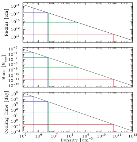
Figure 7: Three properties of the post-shock plasma are shown as a function of the assumed post-shock density, knowing that the emission measure was roughly 2$\times 10^{56}$ cm^-3 during the plateau phase. The top panel shows the radius of a sphere whose total volume is required to explain the observed emission measure. The middle panel shows the total mass of the shocked matter. The bottom panel shows the Bremsstrahlung cooling time for a 4 keV plasma. See text for the explanations of blue, green, and red lines

The delayed ejection models provide estimates of the the inner radius of the absorbing matter as a function of time. Using the version shown in the left panel of Figure 6, the inner radius was 1.5$\times 10^{14}$ cm on Day 61.2 and 5.7$\times 10^{14}$ cm on Day 124.5, times of the two Swift observations that define the plateau phase. These radii are indicated by the horizontal blue lines in the top panel of Figure 7. The vertical blue lines indicate the density that the post-shock plasma needs to have to explain the observed emission measure, if it occupied the entire spherical regions inside these radii. In reality, the post-shock region occupies a fraction of such a sphere, so the true density is to the right of these lines. In the middle and bottom panels, blue lines indicate the total shocked mass and cooling times that are implied by these two limits on the density.

These lower limits on the density allow us to comment on the possibility that the X-ray spectrum may be due to a single-temperature, non-equilibrium ionization plasma. Since $nt\sim 10^{12}$ cm^-3s is the condition to reach ionization equilibrium (Smith & Hughes, 2010), it takes a few days to do so at the beginning of the plateau phase. It is therefore unlikely that non-equilibrium effects are important for our observations of V959 Mon, and justifies our choice of 2 temperature collisional ionization equilibrium model.

Peretz et al. (2016) inferred a 1$\sigma$ density lower limit of the X-ray emitting plasma of 6$\times 10^{10}$ cm^-3 (shown in red in Figure 7), our own analysis suggests this was probably not a secure result. Instead, we rely on the estimates for the density of the inner edge of the torus, obtained by considering the N_H,int evolution, of 3.3 $\times 10^{8}$ and 4.5 $\times 10^{6}$ cm^-3 at Day 60 and 120, respectively (shown in green). For the reverse shock to dominate the X-ray emission throughout the plateau phase, as we argued based on the longevity of this phase, the density of the reverse shock must be lower than that of the inner edge of the torus. This results in the fast flow immediately slowing down, thus ensuring a strong shock. In contrast, the additional momentum provided by the fast flow results only in a small perturbation of the slow torus, so the forward shock makes only a minor contribution to the observed X-rays. This suggests that the density of the reverse shock to be left of the green vertical lines.

We can now use the constraints on the post-shock densities of the reverse shock to infer the mass-loss rate, assuming a spherical outflow with a constant mass-loss rate. A fiducial rate of 1.0 $\times 10^{21}$ g s^-1 would results in post-shock densities of $\sim 4.0\times 10^{7}$ and $\sim 2.5\times 10^{6}$ cm^-3 at Days 60 and 120, respectively. Comparing these estimate with the lower (blue) and upper (green) limits on the post-shock densities of the reverse shock we estimated above, we see that any constant mass-loss rates within a factor of 2–3 of 1.0 $\times 10^{21}$ g s^-1 would have densities that satisfy both limits through days 60–120. Such an outflow implies a shock power of order 10³⁷ erg s^-1, considerably higher than the observed X-ray luminosity, much higher than the observed luminosity of $\sim 6\times 10^{33}$ erg s^-1; this is consistent with the long cooling time inferred for the relatively low densities. For a radiative shock to explain the observed luminosity, one needs the $\sim$1820 km s^-1 matter to be shocked at a rate of roughly 4$\times 10^{17}$ g s^-1. If this was a uniform density, spherical flow, at $r_{\rm in}\sim 1.4\times 10^{14}$ cm (appropriate for Day 60, $t_{e}$=40 d, $v_{\rm in}$=770 km s^-1), the post-shock density is $\sim 3.6\times 10^{4}$ cm^-3. This requires clumps with densities 4 orders of magnitudes higher for such a shock to be radiative, exceeding the estimated density of the inner edge of the torus. This interpretation almost certainly requires small, high density clumps in the fast outflow to collide with high density clumps in the torus, a situation we find unlikely.

4.5 Kinematics of the Two Outflows

The blueshift and the broadening of the emission lines have the potential to confirm, or refute, the scenario outlined above. First we note that the line width is not due to thermal Doppler motions. While the thermal velocity of hydrogen is $\sim$700 km s^-1for a 4 keV plasma, the thermal velocity of an ion scales with the square root of the atomic weight, so it is $\sim$140 km s^-1 for Mg, too small to be the origin of the measured line width. Instead, the line width is due to the bulk motion of ions moving in a variety of directions. The fact that we observe a net blueshift requires that redshifted emission be hidden. In an expanding shell, ions moving away from us are on the far side of the central binary. Therefore, we posit that the unshocked part of the fast outflow at the center of the nova occupies a large enough volume to be able to absorb the redshifted emission on the far side, allowing us to observe only the blueshifted emission on the near side.

If the bulk of the X-rays are emitted by the forward shock driven into the torus, and if the unshocked torus matter is moving outward at 770 km s^-1, then the shock front is traveling outward at an inertial frame velocity of $\sim$2600 km s^-1 (for solar abundances) or $\sim$2100 km s^-1 (for highly metal enhanced case), given kT$\sim$4 keV. The strong shock condition then means that the post-shock, X-ray emitting plasma is moving outward at a velocity of 2150–1750 km s^-1. This does not necessarily imply that we should observe a net blueshift of $\sim$2000 km s^-1: What we observe is the average of projected velocities of all observable parts of the torus, including the part that is moving away from us. The net blueshift can be reduced if more of the torus is observable, while the line width can be reduced if only a small portion is observable: it does not appear feasible to reduce both by absorption.

To assess the expected kinematics of the reverse shock matter, we rely on the measurements of ejecta velocities in the system from optical spectroscopy (maximum expansion velocity of 2400${}^{+300}_{-200}$ km s^-1 according to Ribeiro et al. 2013). If the faster ejecta have this maximum velocity, and the shock velocity is 1820 km s^-1, and if the reverse shock is moving with the inner edge of the slow torus, then the slower material being swept up must be traveling at $\sim$580${}^{+300}_{-200}$ km s^-1. The observed lines would include contributions from the lower-temperature matter in the forward shock, whose bulk outward velocity should be of order $\sim$1000 km s^-1 using a shock temperature of order 0.5 keV and the same argument we used in the previous paragraph. The observed kinematics of the emission regions does not appear to contradict our reverse-shock dominated model, within the limit of the Chandra HETG data. Higher quality X-ray spectroscopy of a future bright nova has the potential to distinguish these two scenarios unambiguously.

4.6 Abundances of the ejecta

As noted in section 3, the abundances we derived using Chandra and Suzaku data do not agree quantitatively. Moreover, while optical spectra (Tarasova, 2014) suggest a high abundance of iron, Suzaku data in particular indicate a lower than solar abundance of iron. Similar tension regarding iron abundance between the optical and X-ray data were noted for V382 Vel (Mukai & Ishida, 2001). Different sensitivity of Chandra and Suzaku data to different features (continuum vs. lines, hard energy bands vs. soft) and different assumptions made during data analysis may in part be responsible. As we argued earlier, this is likely to be the case for the disagreement regarding the abundance of neon, coupled with the disagreement regarding N_H, between Chandra and Suzaku data. However, the X-ray vs. optical disagreements regarding iron abundance, in particular, has now been found in multiple novae. For V382 Vel, Mukai & Ishida (2001) proposed a possible ionization effect, but it may also exist in the X-ray absorber in V906 Car (Sokolovsky et al., 2020).

The disagreements may be due to the chemical inhomogeneity of nova ejecta, created through gravitational settling, diffusion and/or mixing of core material prior to and during thermo-nuclear runaway, and the nuclear reactions during runaway itself. Perhaps abundance differences among different layers can persist in the nova ejecta. Abundance measurements of spatially resolved nova shells would be a great first step in assessing if this is a real effect.

4.7 Implications for gamma-ray emission phase of V959 Mon and other novae

The luminosity of the shock X-ray emission we observe in V959 Mon is below 10³⁴ erg s^-1 ever since the Swift monitoring started. This is similar to those of shock X-rays observed in other novae with dwarf mass donors (i.e., cataclysmic variables; those in symbiotic systems, such as RS Oph, are more luminous; see Mukai et al. 2008) at similar stages of nova eruptions. On the other hand, we have inferred that the X-rays we observe in V959 Mon after Day 60 were probably from a non-radiative shock, and the shock power can be as high as 10³⁷ erg s^-1. While this approaches the shock power needed to explain the gamma-ray luminosity, one would not expect the shock to have been radiatively as inefficient at early times. This is because gamma-ray emission epoch is before the ejection of the torus from the binary, meaning that the shock is much closer to the white dwarf. Therefore, the post-shock density would have been higher, and hence a much higher fraction of the shock power should be emitted promptly as X-rays.

We now have two NuSTAR detections of novae concurrent with Fermi detection of GeV gamma-rays. The thermal X-ray luminosity of V5855 Sgr was found to be a few times 10³³–10³⁴ erg s^-1 for a distance of 4.5 kpc in a single component fit to the NuSTAR spectrum (Nelson et al., 2019). The X-ray luminosity of V906 Car was found to be $\sim$1.5 $\times 10^{34}$ erg s^-1 for a distance of 4 kpc in a single-temperature fit (Sokolovsky et al., 2020). These luminosity values are similar to what we infer for V959 Mon during the observations described here. Moreover, Sokolovsky et al. (2020) found a smooth evolution of X-ray properties from the early times, when the spectrum was so highly absorbed as to be detectable only with NuSTAR, to the later epochs when less absorbed X-rays were detected with Swift. This suggest that the early X-rays, observed concurrently with GeV gamma-ray emission, also originate in the reverse shock.

While the true thermal X-ray luminosity could have been higher in both V5855 Sgr and V906 Car at the time of Fermi detection, if more complex spectral models were considered, such models were not required by the NuSTAR data. In addition, to our knowledge, the only confirmed nova ever detected with all-sky X-ray monitors is RS Oph (with Swift BAT; Bode et al. 2006) even though these all-sky surveys are eminently capable of detecting transient X-ray sources with luminosities of order 10³⁶ erg s^-1 at Galactic center type distances, unless X-ray transients CI Cam and MAXI J0158$-$744 turn out to be nova eruptions as interpreted by several authors (Ishida et al., 2004; Li et al., 2012). These observations are placing an increasingly tighter constraints on the regions of phase space where unseen powerful ($\sim 10^{38}$ erg s^-1) shocks can exist in novae during the gamma-ray emission phase. Optically-thin, thermal X-rays from such shocks can only hide if the temperature was lower than that of the X-rays we do detect later in the life of a nova, so that it can be easily absorbed by a modest absorption column, or if their luminosity decayed rapidly while the absorbing column through the torus is still high.

5 Conclusions

We have analyzed X-ray observations of the Fermi-detected nova V959 Mon obtained with Swift, Chandra, and Suzaku between 60 and 160 days after the start of the eruption. Our major conclusions are as follows:

• The early X-ray evolution observed in V959 Mon is consistent with internal shocks in the ejecta as the fast outflow collides with the slower material in an equatorial torus. This picture is broadly consistent with the what is already known about the nova from radio and optical observations.

• We require a multi-temperature model to explain the line strengths of H- and He-like ions of Mg and other medium-Z elements. We propose that the hotter component, responsible for most of the flux, is from the reverse shock driven into the fast outflow, while the lower temperature component is due to the forward shock driven into the torus.

• The absorption towards the X-ray emitting region drops with time as the ejecta expand and decrease in density. The steep decline of N_H,int observed in the Swift data is not consistent with a shell that expands from $t_{0}$; instead, the decline is better matched by a shell that was ejected from the white dwarf roughly 38 days after the start of the eruption.

• The observed X-ray spectra are consistent with the overabundance of medium-Z elements. If the X-ray absorber has the same non-solar abundances, and allowing for the geometrical factor of the torus, the mass of the shell ahead of the X-ray emitting region is perhaps a few times 10^-6 M_⊙, considerably lower than the radio estimate of the total ejecta mass. We consider the possibility that the torus is clumpy: the radio emission was dominated by the high-density clumps, while the X-ray absorption was dominated by the inter-clump material.

• At the time of the Swift observations, the X-ray emitting shock probably was not radiative. Although the observed X-ray luminosity was modest (below 10³⁴ erg s^-1), the true shock power was likely considerably higher, perhaps 10³⁷ erg s^-1. The inferred shock power is closer to that inferred from the observed gamma-ray luminosity. At early times, the shocked plasma must have had much higher density, which should have resulted in an X-ray luminosity close to the shock power, yet no novae to date have been observed to have such high luminosity X-ray emissions.

Data Availability

The data presented in this article are all publicly available at the High Energy Astrophysics Science Archive Research Center (https://heasarc.gsfc.nasa.gov).

References

- Ackermann et al. (2014) Ackermann M., Ajello M., Albert A., et al., 2014, Science, 345, 554
- Aydi et al. (2020) Aydi E., et al., 2020, Nature Astronomy, 4, 776
- Balman et al. (1998) Balman Ş., Krautter J., Ögelman H., 1998, ApJ, 499, 395
- Bode & Evans (2008) Bode M., Evans A., eds, 2008, Classical Novae, 2nd Edition. Cambridge University Press, Cambridge, UK
- Bode et al. (2006) Bode M. F., O’Brien T. J., Osborne J. P., et al., 2006, ApJ, 652, 629
- Cash (1979) Cash W., 1979, ApJ, 228, 939
- Cheung et al. (2012a) Cheung C. C., Hays E., Venters T., Donato D., Corbet R. H. D., 2012a, The Astronomer’s Telegram, 4224
- Cheung et al. (2012b) Cheung C. C., Shore S. N., De Gennaro Aquino I., Charbonnel S., Edlin J., Hays E., Corbet R. H. D., Wood D. L., 2012b, The Astronomer’s Telegram, 4310
- Cheung et al. (2016) Cheung C. C., Jean P., Shore S. N., et al., 2016, ApJ, 826, 142
- Chomiuk et al. (2014a) Chomiuk L., Linford J. D., Yang J., et al., 2014a, Nature, 514, 339
- Chomiuk et al. (2014b) Chomiuk L., Nelson T., Mukai K., et al., 2014b, ApJ, 788, 130
- Diaz et al. (2010) Diaz M. P., Williams R. E., Luna G. J., Moraes M., Takeda L., 2010, AJ, 140, 1860
- Evans et al. (2014) Evans P. A., et al., 2014, ApJS, 210, 8
- Fujikawa et al. (2012) Fujikawa S., Yamaoka H., Nakano S., 2012, Central Bureau Electronic Telegrams, 3202
- Güver & Özel (2009) Güver T., Özel F., 2009, MNRAS, 400, 2050
- Healy et al. (2017) Healy F., O’Brien T. J., Beswick R., Avison A., Argo M. K., 2017, MNRAS, 469, 3976
- Helton et al. (2012) Helton L. A., et al., 2012, ApJ, 755, 37
- Ishida et al. (2004) Ishida M., Morio K., Ueda Y., 2004, ApJ, 601, 1088
- Li et al. (2012) Li K. L., Kong A. K. H., Charles P. A., et al., 2012, ApJ, 761, 99
- Linford et al. (2015) Linford J. D., Ribeiro V. A. R. M., Chomiuk L., et al., 2015, ApJ, 805, 136
- Metzger et al. (2014) Metzger B. D., Hascoët R., Vurm I., Beloborodov A. M., Chomiuk L., Sokoloski J. L., Nelson T., 2014, MNRAS, 442, 713
- Mukai & Ishida (2001) Mukai K., Ishida M., 2001, ApJ, 551, 1024
- Mukai et al. (2008) Mukai K., Orio M., Della Valle M., 2008, ApJ, 677, 1248
- Munari et al. (2013) Munari U., Dallaporta S., Castellani F., et al., 2013, MNRAS, 435, 771
- Nelson et al. (2012) Nelson T., Donato D., Mukai K., Sokoloski J., Chomiuk L., 2012, ApJ, 748, 43
- Nelson et al. (2014) Nelson T., Chomiuk L., Roy N., et al., 2014, ApJ, 785, 78
- Nelson et al. (2019) Nelson T., Mukai K., Li K.-L., et al., 2019, ApJ, 872, 86
- Ness et al. (2007) Ness J.-U., Schwarz G. J., Retter A., et al., 2007, ApJ, 663, 505
- Ness et al. (2012) Ness J.-U., Shore S. N., Drake J. J., Osborne J. P., Page K. L., Beardmore A., Schwarz G., Starrfield S., 2012, The Astronomer’s Telegram, 4569, 1
- Newville et al. (2014) Newville M., Stensitzki T., Allen D. B., Ingargiola A., 2014, LMFIT: Non-Linear Least-Square Minimization and Curve-Fitting for Python, doi:10.5281/zenodo.11813, https://doi.org/10.5281/zenodo.11813
- O’Brien et al. (1994) O’Brien T. J., Lloyd H. M., Bode M. F., 1994, MNRAS, 271, 155
- Orio et al. (2015) Orio M., Rana V., Page K. L., Sokoloski J., Harrison F., 2015, MNRAS, 448, L35
- Page et al. (2013) Page K. L., Osborne J. P., Wagner R. M., et al., 2013, ApJ, 768, L26
- Pejcha et al. (2016) Pejcha O., Metzger B. D., Tomida K., 2016, MNRAS, 461, 2527
- Peretz et al. (2016) Peretz U., Orio M., Behar E., Bianchini A., Gallagher J., Rauch T., Tofflemire B., Zemko P., 2016, ApJ, 829, 2
- Porquet et al. (2001) Porquet D., Mewe R., Dubau J., Raassen A. J. J., Kaastra J. S., 2001, A&A, 376, 1113
- Ribeiro et al. (2013) Ribeiro V. A. R. M., Munari U., Valisa P., 2013, ApJ, 768, 49
- Schwarz et al. (2011) Schwarz G. J., Ness J.-U., Osborne J. P., et al., 2011, ApJS, 197, 31
- Seaquist & Palimaka (1977) Seaquist E. R., Palimaka J., 1977, ApJ, 217, 781
- Shore et al. (2013) Shore S. N., De Gennaro Aquino I., Schwarz G. J., Augusteijn T., Cheung C. C., Walter F. M., Starrfield S., 2013, A&A, 553, A123
- Smith & Hughes (2010) Smith R. K., Hughes J. P., 2010, ApJ, 718, 583
- Sokoloski et al. (2006) Sokoloski J. L., Luna G. J. M., Mukai K., Kenyon S. J., 2006, Nature, 442, 276
- Sokoloski et al. (2017) Sokoloski J. L., Lawrence S., Crotts A. P. S., Mukai K., 2017, arXiv:1702.05898,
- Sokolovsky et al. (2020) Sokolovsky K. V., et al., 2020, MNRAS, 497, 2569
- Tarasova (2014) Tarasova T. N., 2014, Astronomy Letters, 40, 309
- Verner et al. (1996) Verner D. A., Ferland G. J., Korista K. T., Yakovlev D. G., 1996, ApJ, 465, 487
- Weston et al. (2016) Weston J. H. S., et al., 2016, MNRAS, 457, 887
- Wilms et al. (2000) Wilms J., Allen A., McCray R., 2000, ApJ, 542, 914