MHD accretion-ejection: jets launched by a non-isotropic accretion disk dynamo. I. Validation and application of selected dynamo tensorial components

Abstract

Astrophysical jets are launched from strongly magnetized systems that host an accretion disk surrounding a central object. The origin of the jet launching magnetic field is one of the open questions for modeling the accretion-ejection process. Here we address the question how to generate the accretion disk magnetization and field structure required for jet launching. Applying the PLUTO code, we present the first resistive MHD simulations of jet launching including a non-scalar accretion disk mean-field $\alpha^{2}\Omega$-dynamo in the context of large scale disk-jet simulations. Essentially, we find the $\alpha_{\phi}$-dynamo component determining the amplification of the poloidal magnetic field, which is strictly related to the disk magnetization (and, as a consequence, to the jet speed, mass and collimation), while the $\alpha_{R}$ and $\alpha_{\theta}$-dynamo components trigger the formation of multiple, anti-aligned magnetic loops in the disk, with strong consequences on the stability and dynamics of the disk-jet system. In particular, such loops trigger the formation of dynamo inefficient zones, which are characterized by a weak magnetic field, and therefore a lower value of the magnetic diffusivity. The jet mass, speed and collimation are strongly affected by the formation of the dynamo inefficient zones. Moreover, the $\theta$-component of the $\alpha$-dynamo plays a key role when interacting with a non-radial component of the seed magnetic field. We also present correlations between the strength of the disk toy dynamo coefficients and the dynamical parameters of the jet that is launched.

1 Introduction

Astrophysical jets, consisting of collimated high-speed outflows, are launched from a wide range of astrophysical objects such as young stellar objects (YSO), micro-quasars or active galactic nuclei (AGNs). Although these sources span orders of magnitude in term of extension, time scales and energy scales, it is commonly accepted that these jets are launched from systems that host an accretion disk surrounding a central object (Frank et al., 2014; Hawley et al., 2015; Pudritz & Ray, 2019). Further agreement is on the key role of the large-scale magnetic field for the launching, acceleration and collimation of jets. With launching we denote the transition between accretion and ejection, respectively the mass loading of outflows and jets. Quite a number of studies have investigated this launching process (see, e.g., Blandford & Payne 1982; Uchida & Shibata 1985; Casse & Keppens 2002; Fendt 2006; Zanni et al. 2007; Tzeferacos et al. 2009; Stepanovs & Fendt 2014; Stepanovs et al. 2014; Fendt & Gaßmann 2018).

Still, the origin of the jet-launching disk magnetic field is not completely understood. Analytical models and numerical simulations have so far mostly assumed a predefined large-scale, open magnetic field structure, whose strength and configuration is an essential parameter when understanding and determining the jet dynamics (Murphy et al., 2010; Stepanovs & Fendt, 2016). For the origin of the accretion disk magnetic field one may consider are an extended central stellar magnetic field, the advection of magnetic flux from the ambient interstellar medium, or a magnetic field that is generated by a dynamo process in the disk. The latter scenario is particularly interesting in order to generate jets from AGN, which host as a central object a supermassive black hole, that, unlike stellar objects, cannot produce its own magnetic field.

Disk dynamos have been suggested already some decades ago (Pudritz, 1981a, b; Brandenburg et al., 1995), and there is a huge literature on dynamo theories and their applications to astrophysics (for reviews see e.g. Brandenburg & Subramanian 2005; Rincon 2019). Essentially, astrophysical dynamos are thought to be of turbulent, thus small scale nature, while, on the other hand, one is interested in its large scale effects on the dynamics of these systems. Overall, it is prohibitively expensive to model the turbulence, involving the smallest scales, and, at the same time, aiming to describe astrophysical systems on large scales. The disk turbulence that may lead to both, a turbulent dynamo effect but also to a turbulent magnetic diffusivity is generally thought to be generated by the magneto-rotational instability, MRI (Balbus & Hawley, 1991).

For this reason two paths of modelling dynamos have been pursued. These are (i) direct simulations, which study the natural amplification of the magnetic field (see, e.g., Gressel 2010; Bai & Stone 2013; Gressel & Pessah 2015; Riols, & Latter 2018; Hogg & Reynolds 2018; Dhang et al. 2020), and (ii) the mean-field approach (see, e.g., Krause & Rädler 1980; Rüdiger et al. 1995; Campbell 1999; von Rekowski et al. 2000; Bardou et al. 2001; Chabrier & Küker 2006), by which (iia) (semi-)analytical solution can be derived, or (iib) global numerical simulations can be run covering the large scales of astrophysical systems.

In this paper we follow the second approach. Previous work in this field of large-scale disk-jet simulations and a possible origin of large-scale magnetic field in accretion disks have been performed by von Rekowski et al. (2003); Stepanovs et al. (2014); Fendt & Gaßmann (2018); Dyda et al. (2018), essentially demonstrating that a mean-field dynamo generated magnetic field can efficiently launch jet or outflows. Most recently, mean-field dynamos have also be considered in general relativistic MHD tori (Bucciantini & Del Zanna, 2013; Bugli et al., 2014; Tomei et al., 2020) and disks (Vourellis & Fendt, 2020).

In particular, we extend the work of Stepanovs et al. (2014) by studying the effects of a non-scalar mean-field dynamo. This has not yet been done for launching simulations. By prescribing a non-isotropic dynamo, in the induction equation, we are able to the disentangle the dynamo effects shown in Stepanovs et al. (2014) and Fendt & Gaßmann (2018) in terms of the different components of the dynamo tensor.

Mean-field MHD theory arises from averaging the small-scale dynamics of a turbulent flow pattern, that is (in our case) affected by a central gravity and a subsequent rotation pattern, gas pressure gradients, and Lorentz forces. Both analytical theory (e.g. Rüdiger, & Kichatinov 1993) as well as direct numerical simulations resolving the disk turbulence (e.g. Gressel 2010) have clearly detected an anisotropic nature of the dynamo tensor. As demonstrated by previous work the different tensor components have different amplitudes and different impact on the magnetic field components. We thus believe that the anisotropy of the dynamo will have essential impact on the structure of the dynamo-generated magnetic field. This has not been shown before in a numerical simulation of jet-launching disks.

The paper is organized as follows. In Section 2 we describe our model setup and the numerical approach. In Section 3 we investigate the different effects of the single components of a vectorial dynamo tensor on the jet launching process. We summarize our paper in Section 4. In the Appendix we define our control volumes and provide test simulations comparing our new code to previous works.

2 Model approach

2.1 MHD equations

We solve the time-dependent, resistive MHD equations applying the PLUTO code (Mignone et al., 2007) version 4.3, on a spherical grid $(R,\theta,\phi)$ assuming axisymmetry. We refer to $(r,z,\phi)$ as cylindrical coordinates. The code integrates and solves numerically the set of MHD conservation laws, in particular for the conservation of mass,

$$\frac{\partial\rho}{\partial t}+\nabla\cdot(\rho\mathbf{v})=0,$$ (1)

where $\rho$ and $\mathbf{v}$ are, respectively, the plasma density and the flow velocity; the momentum conservation,

$$\frac{\partial\rho\mathbf{v}}{\partial t}+\nabla\cdot\left[\rho\mathbf{v}\mathbf{v}+\left(P+\frac{\mathbf{B}\cdot\mathbf{B}}{2}\right)\mathsf{I}-\mathbf{B}\mathbf{B}\right]+\rho\nabla\Phi_{\rm g}=0,$$ (2)

where $p$ and $\mathbf{B}$ denote the gas pressure and the magnetic field, respectively. The central object of mass $M$ provides the gravitational potential $\Phi_{\rm g}=-GM/R$. The energy is conserved through the equation

$$\frac{\partial e}{\partial t}+\nabla\cdot\left[\left(e+P+\frac{\mathbf{B}\cdot\mathbf{B}}{2}\right)\mathbf{v}-(\mathbf{v}\cdot\mathbf{B})\mathbf{B}+\overline{\eta}\mathbf{J}\times\mathbf{B}\right]=\Lambda_{\rm{cool}},$$ (3)

where the total energy density is defined as

$$e=\frac{P}{\gamma-1}+\rho\frac{\mathbf{v}\cdot\mathbf{v}}{2}+\frac{\mathbf{B}\cdot\mathbf{B}}{2}+\rho\Phi_{\rm g},$$ (4)

with the polytropic index $\gamma=5/3$.

The electric current density is determined by the Ampere’s law $\mathbf{J}=\nabla\times\mathbf{B}$. As shown e.g. by Casse & Ferreira (2000a); Casse, & Ferreira (2000b); Zanni et al. (2007); Tzeferacos et al. (2013) cooling may play a role in the jet launching process since both density and velocity are subjected to cooling effects. For the sake of simplicity, as in Sheikhnezami et al. (2012); Stepanovs & Fendt (2014), the cooling term is set to be equal to the Ohmic heating, which is, therefore, instantly radiated away.

The magnetic field evolution is determined by the induction equation. Here, we have implemented into the code a mean-field dynamo term (Krause & Rädler, 1980),

$$\frac{\partial\mathbf{B}}{\partial t}=\nabla\times(\mathbf{v}\times\mathbf{B}+{\overline{\alpha}}_{\rm dyn}\mathbf{B}-\overline{\eta}\mathbf{J}),$$ (5)

following mainly the approach of Stepanovs et al. (2014). The tensors ${\overline{\alpha}}_{\rm dyn}$ and $\overline{\eta}$ describe the $\alpha$-effect of the mean-field dynamo and the magnetic diffusivity.

2.2 Numerical setup

As we solve the non-dimensional MHD equations, no intrinsic physical scales are involved. All the primitive MHD variables, i.e. $\rho$,$\mathbf{v}$,$P$,$\mathbf{B}$, as well as the length scale and time scale, are normalized to their value at the initial inner disk radius $R_{\rm{in}}$. Thus, velocities are normalized to $v_{\rm{K,in}}$, corresponding to the Keplerian speed at $R_{\rm{in}}$. As a consequence, the time unit is given in units of $t_{\rm{in}}=R_{\rm{in}}/v_{\rm{K,in}}$, and therefore the quantity $2\pi t_{\rm{in}}$ corresponds to one revolution at the inner disk radius. In the following, all times are measured in units of $t_{\rm{in}}$, implying that $t=2000$ (in short) corresponds to $t=2000\,t_{\rm{in}}$.

The computational domain covers a radial range of $R=[1,100]R_{\rm{in}}$ and an angular range of $\theta=[10^{-8},\pi/2-10^{-8}]\simeq[0,\pi/2]$. A stretched grid is applied in the radial direction considering $\Delta R=R\Delta\theta$. The domain is discretized with a number of $[N_{R}\times N_{\theta}]=[512\times 128]$ grid cells, which allows to resolve the initial disk height $H=0.2r$ with 16 cells.

For the resolution study (see Appendix paper II) we have discretized the domain with $[N_{R}\times N_{\theta}]=[1024\times 256]$ and $[N_{R}\times N_{\theta}]=[256\times 64]$ grid cells, namely 32 and 8 cells per disk height, respectively

Our scale-free simulations may be applied, thus scaled to a variety of jet sources. We apply the same physical scaling as described previous works (Zanni et al., 2007; Tzeferacos et al., 2009; Sheikhnezami et al., 2012; Stepanovs & Fendt, 2014). For an astrophysical scaling of our normalized quantities for typical jet systems we refer to Table 1.

	YSO	BD	AGN	[units]
$R_{0}$	$0.1$	$0.01$	$20$	AU
$M_{0}$	1	0.05	$10^{8}$	$M_{\odot}$
$\rho_{0}$	$10^{-10}$	$10^{-13}$	$10^{-12}$	$g\;cm^{-3}$
$v_{0}$	94	66	$6.7\times 10^{4}$	$km\;s^{-1}$
$B_{0}$	15	0.5	1000	$G$
$t_{0}$	1.7	0.25	0.5	${\rm days}$
$\dot{M}_{0}$	$3\times 10^{-5}$	$2\times 10^{-10}$	$10$	$M_{\odot}yr^{-1}$

Table 1: Typical parameter scales for different sources, in particular Young Stellar Objects (YSOs), Brown Dwarfs (BDs) and Active Galactic Nuclei (AGN)

For spatial integration we use the piecewise parabolic interpolation method (PPM, see Mignone 2014). Time integration is achieved through a third-order Runge-Kutta scheme, while for the flux computation a Harten-Lax-van Leer (HLL) Riemann solver is employed (Toro, 2009). To preserve the the solenoidal condition of the magnetic field, the method of Upwind Constrained Transport (UCT, Londrillo & del Zanna 2004) is applied. In order to achieve stability we choose a Courant-Friedrichs-Lewy time stepping with $CLF=0.4<1/\sqrt{\rm{N_{dim}}}$. This may be a challenge for our diffusive MHD simulations, in particular for high resolution as the diffusive time step goes as $\tau_{\eta}=(\Delta R)^{2}/\eta$.

2.3 Initial conditions

The simulations start with a very weak initial seed field, thus with a very low disk magnetization, defined as the ratio between the magnetic pressure and the thermal pressure $\mu_{\rm{in}}=B_{\rm in}^{2}/P_{\rm in}=10^{-5}$ measured at the disk mid-plane. Therefore, the initial structure of the accretion disk can be obtained as a solution of the hydrostatic equilibrium between thermal pressure gradients, gravity and centrifugal force (Zanni et al., 2007; Stepanovs & Fendt, 2014), neglecting the Lorentz force (Stepanovs et al., 2014; Fendt & Gaßmann, 2018),

$$\nabla P+\rho\nabla\Phi_{\rm g}-\frac{1}{R}\rho v_{\phi}^{2}(\mathbf{e}_{R}\sin\theta+\mathbf{e}_{\theta}\cos\theta)=0.$$ (6)

This equation can be solved assuming that all the quantities $X$ scale as power laws, $X=X_{0}R^{\beta_{X}}F_{X}(\theta)$, where $X_{0}$ is the corresponding quantity evaluated at the innermost radius of the disk (mid-plane). For the sake of clarity we summarize here the pertinent formulas. Self-similarity requires that every characteristic speed should scale as the Keplerian velocity, $\propto R^{-1/2}$. Combining this assumption with a polytropic gas, $P\propto\rho^{\gamma}$, the power law coefficients are $\beta_{u_{\phi}}=-1/2$, $\beta_{\rm P}=-5/2$, and $\beta_{\rho}=-3/2$ (as in the self-similar solution of e.g. Blandford & Payne 1982). A key parameter to describe the initial disk structure is the ratio between the isothermal sound speed and the Keplerian velocity at the disk mid-plane of the inner radius $\epsilon=c_{\rm s}/v_{\phi}\left|{}_{\theta=\pi/2}\right.$. For an initially thin disk, $\epsilon=z/r=0.1$, and solving for the $z$-component of Eq. 6 with $\rho_{\rm{in}}=1$ at the inner disk radius, we obtain

$$F_{\rm P}=\left[\frac{2}{5\epsilon^{2}}\left(1-\frac{1}{\sin\theta}\right)+\frac{1}{\sin\theta}\right]^{5/2},$$ (7)

and where we have chosen $P_{\rm{in}}=0.01$. Following the polytropic relation assumed before, the disk pressure is defined by $F_{\rho}=F_{\rm P}^{3/5}$.

Following Stepanovs & Fendt (2014); Stepanovs et al. (2014), by solving the radial component of Eq. 6 we obtain the disk rotation profile. Outside the disk we define a hydrostatic corona,

$$\rho_{\rm c}=\rho_{\rm{c,in}}R^{1/(1-\gamma)},\,\,\,\,P_{\rm c}=\frac{\gamma-1}{\gamma}\rho_{\rm{c,in}}R^{\gamma/(1-\gamma)},$$ (8)

with $\rho_{\rm{c,in}}=10^{-3}\rho_{\rm in}$. All simulations are initialized with a purely radial magnetic field vanishing outside the disk, defined by the vector potential

$$\mathbf{B}=\nabla\times A\mathbf{e}_{\phi}=\nabla\times\left[\frac{B_{\rm{p,in}}}{r}\exp\left(-8\left(z/H\right)^{2}\right)\right]\mathbf{e}_{\phi}.$$ (9)

Here, $B_{\rm{p,in}}=\epsilon\sqrt{2\mu_{\rm{in}}}$ defines the strength of the initial poloidal magnetic field and $\mu_{\rm{in}}=10^{-5}$ is the initial magnetization along the disk mid-plane. The quantity $H=2\epsilon r$ represents the geometrical disk height, respectively twice the initial pressure scale height.

2.4 Boundary conditions

The boundary conditions are identical to those of Stepanovs & Fendt (2014). We report them in this section for convenience. Along the rotational axis and the equatorial plane the standard symmetry conditions are applied. The inner radial boundary is divided into two different areas. One is the area that is suited for disk accretion located at $\theta>\pi/2-2\epsilon$, the other is the coronal area at $\theta<\pi/2-2\epsilon$, where we choose $2\epsilon\approx\arctan(2\epsilon)$. The boundary condition along the inner radial boundary is essential for stabilizing the corona against collapse to the central object. While $v_{\theta}=0$ along the inner disk boundary, the radial velocity follows a power law, $v_{R}=v_{R_{\rm{in}}}R^{-1/2}\leq 0$, where the inequality is imposed in order to enforce the boundary behaving as a ”sink”. Along the coronal area, we prescribe a constant inflow velocity into the domain $v_{\rm p}=0.2$ (in units of the Keplerian speed at $R_{\rm in}$) in the radial direction, that could be interpreted astrophysically as a stellar wind.

From previous jet formation simulations (see e.g. Ouyed & Pudritz 1997) we expect the terminal jet speed to reach the Keplerian velocity at the inner disk. For $v_{\phi}$ we prescribe a power law across the inner boundary (for both the disk and the coronal boundary)

$$v_{\phi}=v_{\phi}\big{|}_{R_{\rm{in}},R_{\rm{out}}}R^{-1/2}.$$ (10)

The boundary conditions for the poloidal magnetic field along the inner radial boundary obey the divergence-free condition. The method of constrained transport requires to define only the $\theta$-component of the magnetic field along the boundary, while the radial component is recovered from the Maxwell equations. At the outer boundaries both $B_{\phi}$ and $B_{\theta}$ follow a power law

$$B_{\phi,\theta}=B_{\phi,\theta}\big{|}_{\rm{out}}R^{-1},$$ (11)

while $B_{R}$ is again recovered using the solenoidality condition. This is compatible with a constant gradient condition. For the $B_{\phi}$ this implies in particular the conservation of the electric current across the boundary.

Along the inner boundary we prescribe $B_{\phi}=0$ towards the coronal region, while we again adopt a power-law $\propto R^{-1}$ for the boundary area towards the inner disk. Along the inner radial disk boundary, we prescribe the poloidal magnetic field inclination, choosing an angle

$$\varphi=70\degree\left[1+\exp\left(-\frac{\theta-45\degree}{15\degree}\right)\right]^{-1},$$ (12)

where $\varphi$ is the angle of the magnetic field with respect to the disk surface. Note that here again we solve for the divergence-free condition of the magnetic field, recovering the solution with the inclination prescribed.

These boundary conditions are slightly different from Stepanovs et al. (2014) and Fendt & Gaßmann (2018), as we not suppress the advection of magnetic flux from the inner disk towards the axis. This inner boundary condition is known to be quite critical for the numerical stability of the simulation, as it is time-dependent, thus implementing a feedback loop from the cells of active domain. While the boundary condition as defined in the papers mentioned above was chosen because it was found to be less prone to numerical instabilities, for the present paper, we decided to release that boundary condition and allow to advect magnetic flux across the boundary towards the axial region. The advection of flux towards the axis has some impact for the structure of this innermost area, but does not change the structure and the evolution of the surrounding disk jet which is our major focus. We also think that the advection of magnetic flux towards the axis is a more physical boundary condition.

Across the inner and outer boundaries both the density and the pressure are extrapolated by a power law,

$$\rho=\rho\big{|}_{R_{\rm{in}},R_{\rm{out}}}R^{-3/2}\qquad P=P\big{|}_{R_{\rm{in}},R_{\rm{out}}}R^{-5/2},$$ (13)

where $R_{\rm{in}}$ and $R_{\rm out}$ is the inner and the outer radius of the domain. Along the outer boundaries we apply the standard PLUTO outflow (zero gradient) conditions. In addition, we still prescribe $v_{R}$ to be non-positive in the disk region and non-negative in the coronal region.

2.5 The dynamo model

For a thin disk, the non-diagonal components of the mean-field dynamo tensor are negligible. In our approach we consider the explicit form of the dynamo terms following Rüdiger et al. (1995); von Rekowski et al. (2000),

$${\overline{\alpha}}_{\rm dyn}=(\alpha_{R},\alpha_{\theta},\alpha_{\phi})=-\overline{\alpha}_{0}c_{\rm s}F_{\alpha}(z),$$ (14)

where $c_{\rm s}$ is the adiabatic sound speed at the disk mid-plane and $F_{\alpha}(z)$ is a profile function,

$$F_{\alpha}(z)=\left\{\begin{array}[]{ll}\sin\left(\pi\displaystyle\frac{z}{H}\right)&z\leq H\\ \vskip 6.0pt plus 2.0pt minus 2.0pt\cr 0&z>H\end{array}\right.$$ (15)

(Bardou et al., 2001), that confines the dynamo action within the accretion disk. Note that Rüdiger et al. (1995) have applied a slightly different profile, namely a linear function $F_{\alpha}(z)=z/H$ in the disk. We prefer the approach of Bardou et al. (2001) that effectively avoids the discontinuity at the disk surface and is thus better suited for a simulation that includes also the disk corona.

As in Stepanovs et al. (2014), we choose a radial dependence of the dynamo $\alpha\propto R^{-1/2}$, since this profile follows also the sound speed. Note, however, that compared to our former simulations, in the present setup the radial profile of the dynamo is not necessarily constant in time. As the sound speed is included in the dynamo tensor, along with the disk sound speed, also the dynamo tensor is updated every time step. We will demonstrate that this variation has only a minor impact on the overall evolution of the system. However, it represents a more consistent approach and is furthermore in agreement with the analytical models of mean-field dynamo theory (Rüdiger, & Kichatinov, 1993; Rüdiger et al., 1995).

2.6 The diffusivity model

For the magnetic diffusivity tensor we assume a diagonal structure (as for the dynamo). We adopt an $\alpha$-prescription as typically applied in our previous work (Stepanovs et al., 2014),

$$\overline{\eta}=(\eta_{R},\eta_{\theta},\eta_{\phi})=\overline{\eta}_{0}\alpha_{\rm{ss}}c_{\rm s}HF_{\eta}(z),$$ (16)

where $c_{\rm s}$ is the adiabatic sound speed at the disk mid-plane, $H$ is the initial disk pressure scale height while $\alpha_{\rm{ss}}$ is the dimensionless parameter of turbulence (Shakura & Sunyaev, 1973). Thus, the diffusivity is assumed to be essentially of turbulent nature most probably caused by the MRI (Balbus & Hawley, 1991). Again we define a profile function,

$$F_{\eta}(z)=\left\{\begin{array}[]{ll}1&z\leq H\\ \vskip 6.0pt plus 2.0pt minus 2.0pt\cr\exp\left[-2\left(\displaystyle\frac{z-H}{H}\right)^{2}\right]&z>H\end{array}\right.$$ (17)

that confines the diffusivity within the disk region. Note that the magnetic diffusivity, or resistivity, respectively, is motivated here as caused by the disk turbulence, thus much stronger than the microscopic value.

In the literature of jet launching simulations (see e.g. Jacquemin-Ide et al. 2019) without a mean-field dynamo, the magnetic diffusivity is usually computed as

$$\overline{\eta}=\overline{\eta}_{0}v_{\rm A}HF_{\eta}(z),$$ (18)

where the two model approaches described above coincide if $\alpha_{\rm{ss}}=\sqrt{2\mu_{\rm D}/\gamma}$ where $\gamma$ is the polytropic index and $\mu_{\rm D}$ is the magnetization computed at the disk midplane. This model approach, in the following denoted as the standard diffusivity model, is, however, not used in this paper. One reason is that we want to avoid the accretion instability to occur (Campbell, 2009). This can be avoided when the feedback between the magnetization and the magnetic diffusivity is chosen stronger than $\alpha_{\rm{ss}}\propto\sqrt{\mu}$ (see our previous work Stepanovs & Fendt 2014). Note that we already have a feedback loop on the magnetic diffusivity, as the growth of the magnetic field is naturally related to the mean-field dynamo.

We therefore apply the so-called strong diffusivity model that we have previously invented (Stepanovs & Fendt, 2014; Stepanovs et al., 2014),

$$\alpha_{\rm{ss}}=\sqrt{\frac{2}{\gamma}}\left(\frac{\mu_{D}}{\mu_{0}}\right)^{2},$$ (19)

where $\mu_{0}=0.01$. Since the initial magnetic field does not intersect the disk mid-plane, for the quantity $\mu_{\rm D}$ we calculate the ratio between the average total magnetic field (vertically averaged at a certain radius) in the disk and the gas pressure at the disk mid-plane (Stepanovs et al., 2014). As demonstrated previously, this approach allows to perform a more stable evolution of the disk-jet structure over long simulation time (Stepanovs et al., 2014; Fendt & Gaßmann, 2018).

2.7 Dynamo number and dynamo quenching

The dynamo number is the leading parameter for the evolution of the mean-field dynamo-generated magnetic field. Sub-critical dynamo numbers support a slow, linear growth of the magnetic field, while super-critical numbers lead to a rapid, thus exponential growth of the magnetic field. This exponential growth must be quenched by a physical model that damps the dynamo action (thus the dynamo number) for strong fields by first principles. We define the dynamo number as

$${\cal D}=\displaystyle\frac{\alpha_{\phi}\Omega H^{3}}{\eta_{\rm{disk}}^{2}}$$ (20)

(Rüdiger et al., 1995; von Rekowski et al., 2000). Since at $z=H$ the dynamo components vanish, the quantity $\alpha_{\phi}$ is computed at $z=H/2$. For the definition of an average disk diffusivity $\eta_{\rm{disk}}$ we refer to Appendix B .

This definition of the dynamo number is a product of the azimuthal magnetic Reynolds number ${\cal R}_{\Omega}=|\Delta\Omega|H^{2}/\eta_{\rm{disk}}$ based on the shear of the flow $\Delta\Omega$, and the magnetic Reynolds number ${\cal R}_{\alpha}=\alpha_{\phi}H/\eta_{\rm{disk}}$, based on the $\alpha$-effect (considering $\alpha_{\phi}$ as the strongest dynamo contribution in disks).

As demonstrated by Stepanovs et al. (2014), both the disk orbital velocity and the sound speed at the disk mid-plane undergo some little variation during the temporal evolution of the system. Therefore, for an almost constant diffusivity profile with radius, $\cal D$ would scale almost linearly with the radius. We note that this is a rough estimate - as the disk diffusivity does not follow a constant radial profile, even in quasi-steady state.

The dynamo number also depends on $\alpha_{\rm{ss}}$,

$${\cal D}\propto\alpha_{\rm{ss}}^{-2}\propto\mu_{\rm{disk}}^{-4}$$ (21)

(Stepanovs et al., 2014; Fendt & Gaßmann, 2018). Note that our diffusivity model leads to a rapid growth of the magnetic diffusivity and, as a consequence, to a saturation of the magnetic field strength. We thus expect the dynamo number to converge to a sub-critical strength - at a given radius - at which the magnetic field cannot be amplified anymore. In order to determine such a critical strength for dynamo action involves to consider the full nonlinear evolution of the system, and therefore will be subject of analysis in the following sections.

As previously shown (Stepanovs et al., 2014), our diffusivity model is able to suitably quench the dynamo action, preventing an endless amplification of the magnetic field. This is triggered by the strong feedback of the disk magnetization on the magnetic diffusivity (through $\alpha_{ss}$).

Although this model prevents the accretion instability described in Stepanovs & Fendt (2014), it may lead to un-physically large values of $\alpha_{\rm{ss}}$, if not treated with care. Other quenching models, as e.g. the standard quenching model discussed in Rüdiger, & Kichatinov (1993); Rüdiger et al. (1995), lead to the same quenching effect as our diffusive quenching model, while keeping the maximum strength of $\alpha_{ss}$ in a physically likely range as discussed in e.g. King et al. (2007).

However, in order to be able to evolve the long-term properties of the various dynamo models we choose the diffusive quenching over the standard quenching. The standard quenching was found to be prone to the accretion instability for our setup. Furthermore, the diffusive quenching works much smoother compared to the standard quenching and leads to the same result. We note that we do not put any lower bounds on the turbulence level $\alpha_{\rm{ss}}$. This may effect, via the dynamo-alpha $\alpha_{0}$, the critical dynamo number, above which we expect an effective magnetic field amplification. The study of physically more self-consistent feedback models for dynamo quenching will be subject of our future work.

3 A toy model for an anisotropic mean-field dynamo

This section aims to disentangle the effects that are physically caused by the different components of the dynamo tensor (the three components of a vector in our case) in order to gain a detailed understanding of the physical process of field amplification at act.

3.1 Anisotropic dynamo and diffusivity coefficients

Our aim is to generalize the dynamo models applied previously (von Rekowski et al., 2003; Stepanovs et al., 2014; Fendt & Gaßmann, 2018). These works applied a scalar (thus isotropic) $\alpha$ coefficient. Here we apply the anisotropy of the dynamo, assuming that the coefficients $\overline{\alpha}_{0}$, as described in Section 2.5, are not necessarily the same (Rüdiger et al., 1995).

Table 2: Simulations with the dynamo coefficients of $\overline{\alpha}_{0}=(\phi,\psi,\chi)\alpha_{0}$. The magnetic diffusivity distribution is the same with $\eta_{0}=0.165$. The run time of the simulations is $t_{\rm F}$ in units of $1000$.

run ID	$\phi$	$\psi$	$\chi$	$t_{\rm F}$	Comment
Scalar	1.0	1.0	1.0	30	as Stepanovs et al. (2014)
phi_A	1.0	1.0	2.0	10	strong amplification
phi_B	1.0	1.0	0.5	10	weak amplification
phi_C	1.0	1.0	0.1	10	very weak amplification
R_A	2.0	1.0	1.0	10	magnetic loops at $R\simeq 40$
R_B	0.75	1.0	1.0	10	magnetic loops at $R\simeq 20$
th_A	1.0	5.0	1.0	10	multiple loops in $R\in[15,80]$
th_B	1.0	0.1	1.0	4	magnetic loops at $R\simeq 15$

The role of the diffusivity has been widely discussed in the literature (Zanni et al., 2007; Sheikhnezami et al., 2012). Here we assume

$$\overline{\eta}_{0}=\left(\frac{1}{2},\frac{1}{2},1\right)\eta_{0},$$ (22)

where $\eta_{0}=0.165$ recovers the reference values of Stepanovs et al. (2014). In order to have a direct comparison with the simulations of Fendt & Gaßmann (2018), we set the dynamo tensor components as

$$\overline{\alpha}_{0}=(\phi,\psi,\chi)\alpha_{0},$$ (23)

with $\alpha_{0}=0.775$. Setting $\psi=\phi=\chi=1$, we recover the reference simulation of Fendt & Gaßmann (2018).

The strength of the dynamo coefficients $(\phi,\psi,\chi)$ are summarized in Table 2. From this set of simulation runs, we will consider a sample of eight exemplary runs in order to disentangle the influence of the different components of the alpha tensor on the magnetic field structure and the disk and jet evolution.

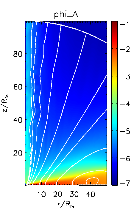
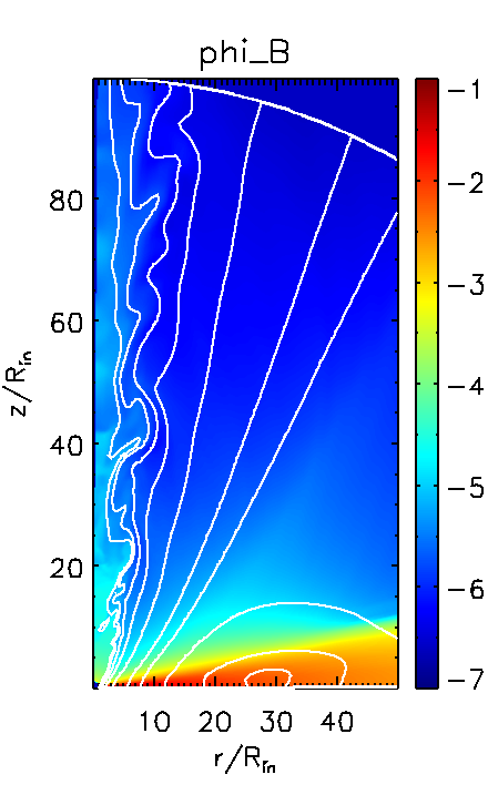
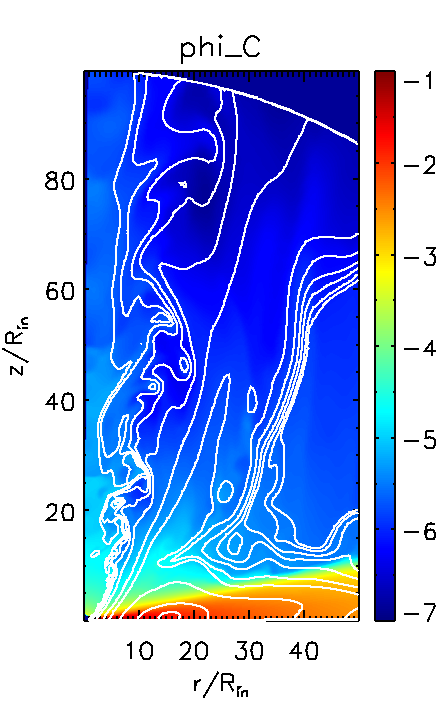
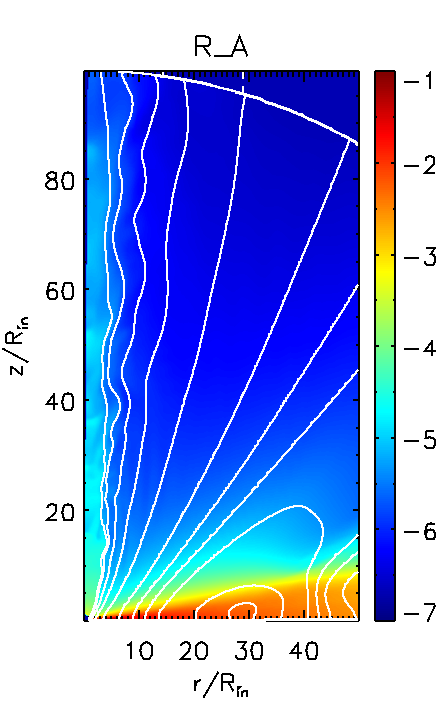
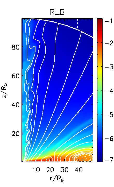
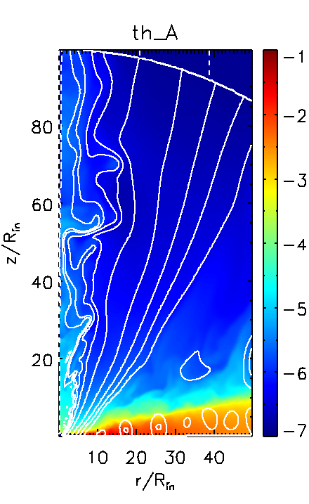
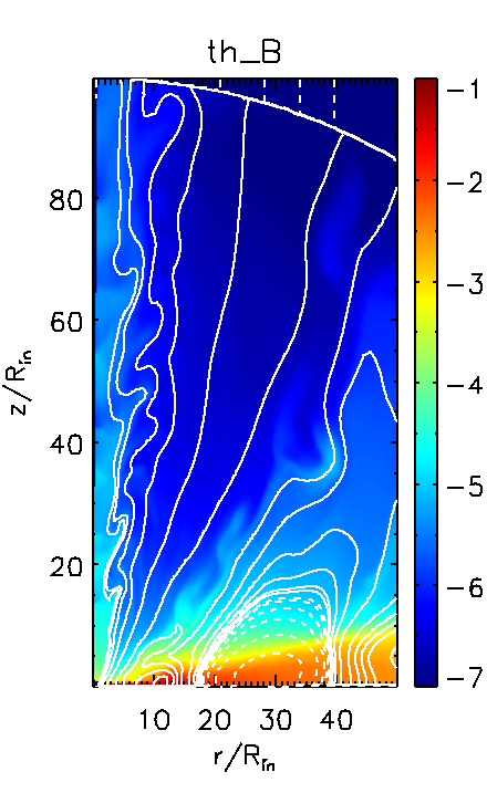
Figure 1: Magnetohydrodynamic evolution of the toy model dynamo simulations (see Table 2 at $t=4000$. Shown is the density distribution (color) and magnetic field lines (white lines). The poloidal magnetic is field is represented by the contour lines of the vector potential $A_{\phi}$. The dashed lines indicate a negative polarity of the poloidal magnetic field.

3.2 Evolution of the magnetic field

Figure 1 shows for the different parameter runs the density distribution of the disk-jet structure, together with the magnetic field geometry (as contour lines of the vector potential). We point out that in all cases but simulation th_B (which is described more in detail in Section 3.4), the initial magnetic field has the radial structure as described in Section 2.3.

Overall, we see that in all simulation runs the magnetic field in the inner region close to the rotation axis that has been generated by dynamo action shows a large scale open geometry. Together with a substantial strength, this magnetic field structure is able to eject disk material in to an outflow with a high degree of collimation. On the other hand, we also see that the very field structure depends on the choice of the dynamo tensor, thus the strength of the tensor components. The choice of different coefficients $(\phi,\psi,\chi)$ in our toy dynamo model leads to a different magnetic field configuration.

3.2.1 A super-critical poloidal dynamo

The induction equation tells us that the dynamo action governed by $\alpha_{\phi}$ is the only way to increase the poloidal magnetic field up to the strength that is required for jet launching. Even for $\alpha_{\phi}=0$ the toroidal magnetic field is still dynamo-amplified through the $\Omega$ effect and also the $\alpha_{R}$ dynamo component. However, the dynamo does not lead to a substantial amplification of the poloidal magnetic field. Therefore the latter cannot increase and stays confined within the disk. Neither the strength nor the launching angle can be reached that is required to produce a Blandford-Payne outflow.

On the other hand, as a consequence of the quenching model applied, the magnetic diffusivity still increases as the toroidal magnetic field growths. As a consequence, the poloidal magnetic field still evolves, even if the field is not enhanced by the dynamo action. Note, however, that even if $\chi>0$, if $\alpha_{\phi}$ is under a critical strength $\alpha_{\rm{crit}}$, the dynamo action for the poloidal field is still negligible.

When comparing the time scales for diffusion and dynamo action for different strength for $\alpha_{\phi}$ (see Fendt & Gaßmann 2018), we find a critical value of $\alpha_{\rm{crit}}\simeq 0.003$, corresponding to $\chi\simeq 0.03$.

Because of the diffusivity model applied in these simulations, we find that the dynamo number is not an unambiguous measure for the initial critical dynamo action, as the disk diffusivity does not only depend on the poloidal magnetic field (that is not amplified as the dynamo $\alpha_{\phi}$ is sub-critical), but also on the toroidal magnetic field (that remains amplified by the dynamo $\alpha_{R}$ and by the $\Omega$ effect). Moreover, as shown in Stepinski & Levy (1988, 1990); Torkelsson & Brandenburg (1994), the initial critical dynamo number depends on several factors e.g. the number of grid cells or the magnetic field configuration. Nevertheless, the dynamo number still remains a key parameter in order to understand the evolution and saturation of the dynamo action (see Sect. 2.7).

For $\alpha_{\phi}<\alpha_{\rm{crit}}$, the poloidal magnetic field increases only by less than one order of magnitude in the outer disk before time $t=3000$, while the inner disk region is not at all magnetically amplified. For $\alpha_{\phi}>\alpha_{\rm{crit}}$, the dynamo effect substantially amplifies the poloidal magnetic field, as shown in Fig. 2, changing both its strength and geometry which subsequently may lead to an disk outflow of material similar to Stepanovs et al. (2014). All the cases that we investigated and that are listed in Table 2 satisfy the condition $\alpha_{\phi}>\alpha_{\rm{crit}}$.

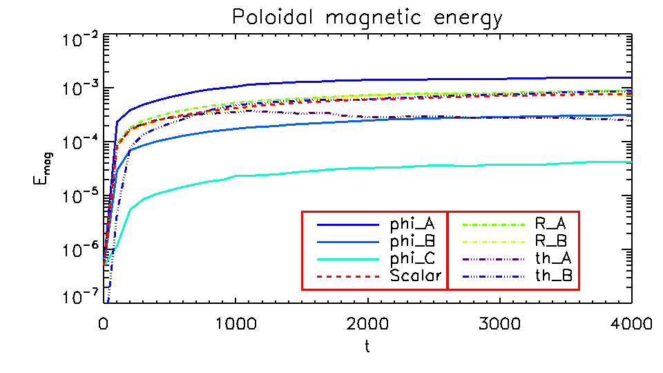
Figure 2: Temporal evolution of the disk poloidal magnetic energy integrated from radius $R=10$ to the end of the domain, $R_{\rm{out}}=100$.

3.2.2 Induction of multiple magnetic loops

Dynamo action triggered by the $\phi$-component of the alpha tensor leads to a topological magnetic field structure such that the magnetic field loops generated in the inner disk region open up and drive a collimated outflow (see also Fig. 1, but also Stepanovs et al. 2014; Fendt & Gaßmann 2018). Outside this inner jet launching region, magnetic loops are continuously formed. This loop structure, that is basically corresponding to a reversal in the radial field $B_{R}$, is diffusing outwards due to the radial magnetic field pressure gradient of the inner disk. Such loops do not correspond to a reversal in the toroidal field and since they are diffused away, their impact on the jet dynamics is negligible.

In case of dynamo action that is substantially an-isotropic (as our cases R_A, R_B and th_A), we observe an essentially different evolution of the magnetic field topology. That is, for $\phi<0.8$ or $\phi>1.5$, a second magnetic loop is formed that is anti-aligned to the loop structure induced further in. These loops, characterized by a reversal in the toroidal field, are substantially different from the ones described previously, and play a significant role in the evolution of the magnetic field and of the disk-jet system (see our discussion below). We point out that the anti-aligned magnetic loops can be formed also when considering a scalar dynamo tensor, when the scalar $\alpha_{0}<0.6$ (Fendt & Gaßmann, 2018).

As shown in Section 3.2.1, the coupling between the toroidal magnetic field and the dynamo tensor component $\alpha_{\phi}$ is the main mechanism responsible for generation of the poloidal field. For $0.8<\phi<1.5$, the toroidal magnetic field, being amplified by the $\Omega$-effect from the radial weak seed field, shows a monotonous behavior (after being amplified). As the system evolves, the poloidal field is amplified over the whole accretion disk.

By looking at the spatial and temporal numerical derivatives of the toroidal field, we find that because of the highly anisotropic character of $\alpha_{R}$, some ”dynamo-inefficient zones” are formed. These are areas of vanishing poloidal field strength, but, in addition, in such zones also the toroidal magnetic field cannot be amplified. The number and the location of these zones, where the dynamo is not efficient, depends on the strength of the three dynamo components and not exclusively by $\alpha_{R}$.

Furthermore, for $\alpha_{\theta}>3$, we find that the toroidal field shows multiple dynamo-inefficient zones. On the other hand, the dynamo-inefficient zones of case th_A remain confined in the accretion disk. This is illustrated in the top panels of Fig. 3 where we show the disk magnetization at the same evolutionary time, $t=4000$. The difference between between the three simulation runs Sc, R_B, and th_A is clearly visible.

For the case of the scalar dynamo the local disk magnetization is only weakly dependent on the radius. It is relatively low along the mid-plane and increases towards the disk surface. This is understandable as the disk gas pressure decreases with altitude while the poloidal field remains rather constant vertically.

For simulation run R_B, for which $\alpha_{R}=0.75$, we see that a dynamo-inefficient zone has developed around radius $R\simeq 23$. Typically, these zones seem to be anchored at the disk mid-plane. As they are balanced by a low magnetic pressure, they vertically extend while preserving the total pressure equilibrium.

For simulation run th_A, for which $\phi=1$ and $\psi=5$, we find multiple dynamo-inefficient zones along the accretion disk. Note that due to their proximity, these zones are able to connect – and reconnect.

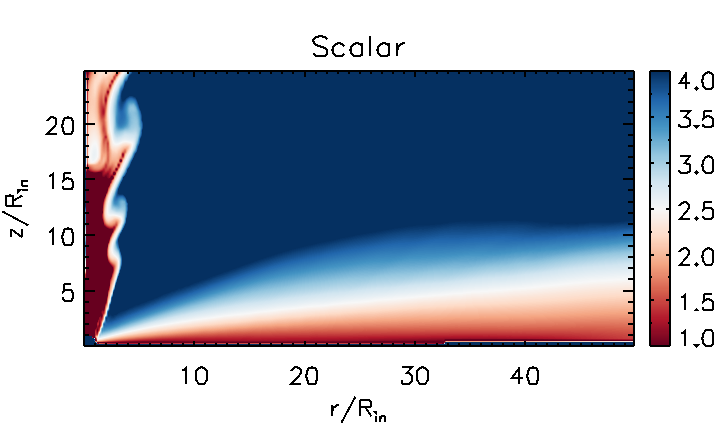
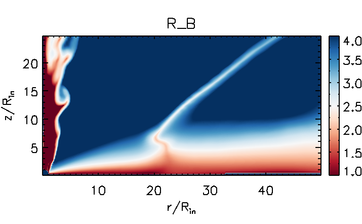
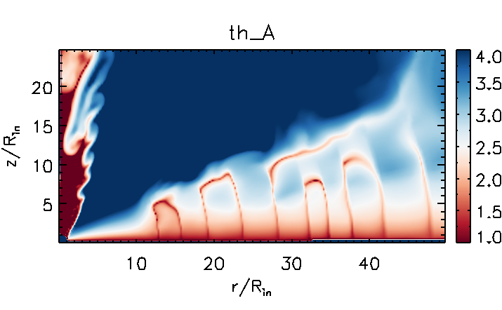
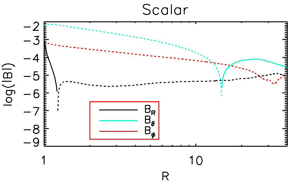
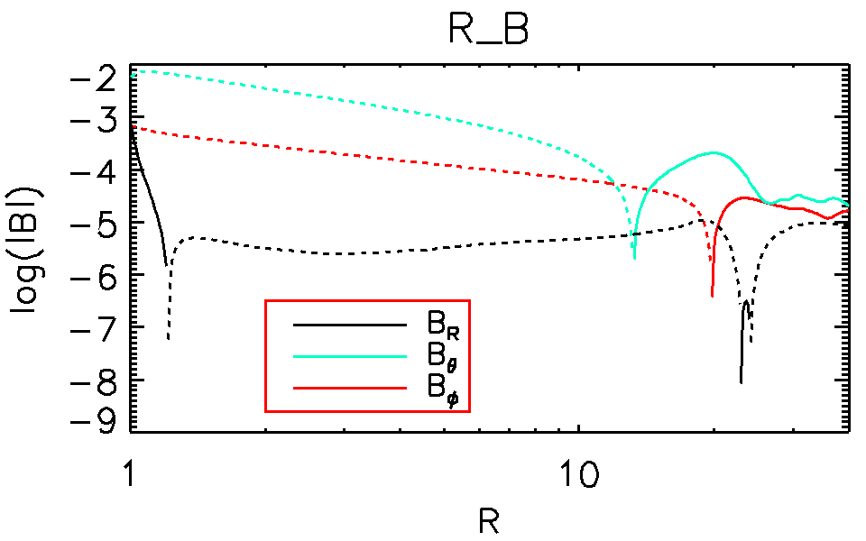
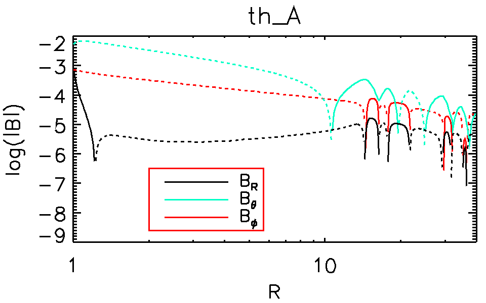
Figure 3: Presence and absence of dynamo-inefficient zones in the disk for different dynamo prescriptions, Scalar (left panels, R_B (middle panels), and th_A (right panels), respectively. The top row shows the disk magnetization at time $t=4000$, while in the bottom row shows the three magnetic field components close to the disk mid-plane at time $t=1000$, where the solid lines represent positive values of the magnetic field and the dashed lines represent negative values of the magnetic field.

Because the coupling between the toroidal field and the $\alpha_{\phi}$-component of the dynamo tensor is the only way to dynamo-amplify the radial field component, the radial field that is amplified from the toroidal has also different polarities.

Since we have physical resistivity included, the magnetic field is able to reconnect and to change its topology within the accretion disk. In particular, instead of one magnetic loop that is visible (see Fig. 3, bottom right panel), now more magnetic loops arise (see Fig. 3, bottom left panel). On the other hand, the reversal of the toroidal field is associated with a maximum in the tensor component $\alpha_{\theta}$, which undergoes a reversal at smaller radii (bottom left panel of Fig. 3).

Compared to the results of Fendt & Gaßmann (2018), here we find that the re-configuration of the magnetic field structure does impact the jet evolution on a weaker level. We believe that this is mainly due to the mid-plane boundary condition, that is absent in the previous paper. In particular, here we enforce symmetry between upper and lower hemisphere that can be violated in a bipolar setup. However, the reversal of the toroidal and radial field components that directly define the disk magnetization still play a key role in the disk-jet evolution. We note that the disk magnetization is the main ingredient of the diffusivity model for the resistive disk evolution.

Since the dynamo-inefficient zones correspond to zones of low diffusivity, as a result the accretion process can be affected. In fact, accretion can be suppressed across such zones, leading to under-dense and over-dense regions (compared to the simulations without multiple loops). We find that these under-dense/over-dense regions are strongly related to the existence of a vertical field. We experienced numerical issues when under-dense zones are located too close to the inner boundary, for example unphysical values of the fluid density or the fluid pressure.

Here we need to comment briefly on the ”dead zones” that has been proposed for protoplanetary disks. Although the dynamo-inefficient zones we detect in our simulations may look similar to these dead zones, the physical processes involved are not the same. Dead zones in protoplanetary disks have been proposed by Gammie (1996) on the basis of a lack of coupling between matter and magnetic field due to an insufficient degree of ionization. This lack of coupling would not allow the MRI to operate, and, as a consequence, also accretion unlikely to happen, since the lack of angular momentum exchange. As a result, a layered accretion is expected on a theoretical basis, which could indeed be realized in numerical simulations (Fleming et al., 2000; Fleming & Stone, 2003). Also, resistivity was found to play an essential role in suppressing the MRI (see e.g. Sano et al. 2000; Fromang et al. 2002; Flock et al. 2012). Dead zones in protoplanetary disk are also thought to be responsible to create transition disks (Pinilla et al., 2016).

It is interesting to note that for both the protoplanetary dead zones and for our dynamo-inefficient zones the resistivity plays a leading role. However, for the first approach it is the resistive de-coupling which suppresses the MRI (and would subsequently suppress the dynamo action of the MRI), while for our models the dynamo-inefficient zone is formed as result of a minimum of the magnetic diffusivity.

Finally we note that as the dynamo-efficient zones are basically resulting from the feedback of the magnetic field on the magnetic diffusivity, a change in the quenching model – from the diffusive quenching to the standard quenching – may affect the exact location and width of the dynamo-inefficient zones.

3.2.3 Amplification of the magnetic field

The majority of our parameter runs apply a super critical dynamo $\alpha_{\phi}>\alpha_{\rm{crit}}$ (Table 2). The resulting magnetic field strength and geometry supports a collimated outflow. In Fig. 2 we show the time evolution for the disk poloidal magnetic energy, integrated from $R=10$. For a comparison the case of an isotropic dynamo is shown.

The three different dynamo tensor components play a different role in the amplification of the poloidal magnetic field. The $\phi$-component of the dynamo is the main ingredient that amplifies the poloidal magnetic field in the disk, while the $R$ and $\theta$-components determine the formation of the dynamo-inefficient zones, that, subsequently, also determines the poloidal magnetic field structure.

The $\phi-$component of the dynamo tensor essentially influences already the very early stages of the disk-jet evolution – a higher strength of $\alpha_{\phi}$ leads to a faster and stronger amplification, as we can see by comparing the ”phi”-simulations to the isotropic model in Fig. 2.

The other dynamo components ($\alpha_{R}$ and $\alpha_{\theta}$) become important only once the poloidal field has been amplified to substantial strength, and through the presence (or absence) of the dynamo-inefficient zones. In particular, where a dynamo-inefficient zone is built up in the inner disk, it triggers the temporal evolution of the system already on short timescales ($\simeq 100$ after its formation ). A dynamo-inefficient zone located further out plays a minor role during the early phase of the disk evolution.

We emphasize that the evolution of the disk magnetic field is strictly correlated with the existence of dynamo-inefficient zones, since these features lead to the formation of multiple anti-aligned magnetic loops in the disk (see Fig. 1 and section 3.2.2). A higher strength of the dynamo tensor component $\alpha_{R}$ leads to an – on average – higher amplification of the toroidal field. However, once the dynamo is quenched by magnetic diffusivity, the magnetic field strength decreases to the magnitude that we recovered in the isotropic dynamo simulation. Therefore, we interpret that the effect of a higher $\alpha_{R}$ is a more rapid amplification of the poloidal field. On the other hand, a lower $\alpha_{R}$ leads to a slower toroidal (and therefore poloidal) field amplification.

We find a different behavior when a dynamo-inefficient zone (only one) is forming which extends beyond the accretion disk surface. As discussed in Section 3.2.2, the reversal of the toroidal field corresponds to a spatially stationary point in the $\theta-$component of the magnetic field. As a result, the poloidal magnetic energy is higher than for the isotropic dynamo model, simply because in the dynamo-inefficient regions of the disk the vertical field component becomes stronger.

On the other hand, this increase in the vertical component of the magnetic field is partially suppressed in the presence of multiple magnetic zones, compared to the case of an isotropic dynamo tensor. Our understanding of this effect is that the existence of quite a number of field reversals (that effectively decrease of the local magnetic energy), more than compensates the induction of a vertical field component (that would lead to a decrease of the local magnetic energy).

3.2.4 The dynamo number

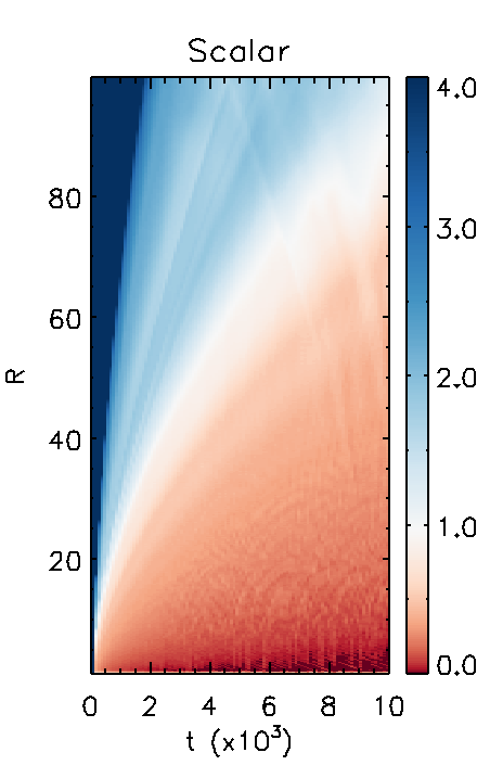
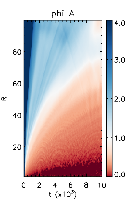
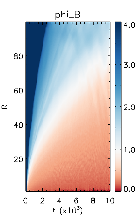
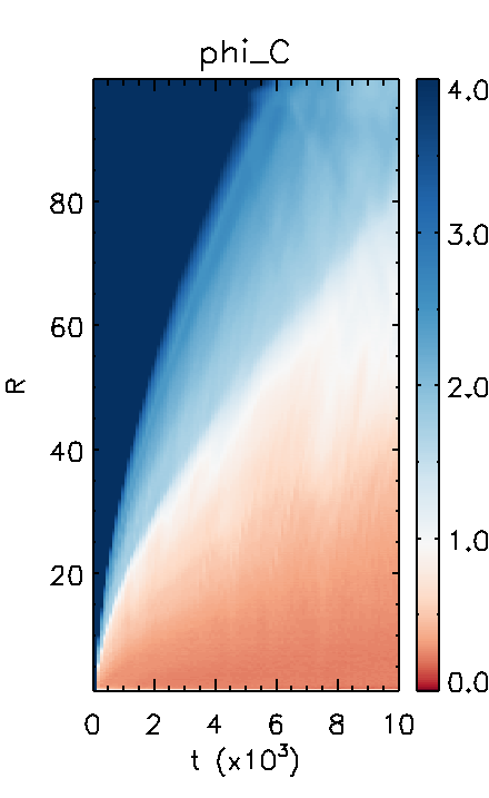
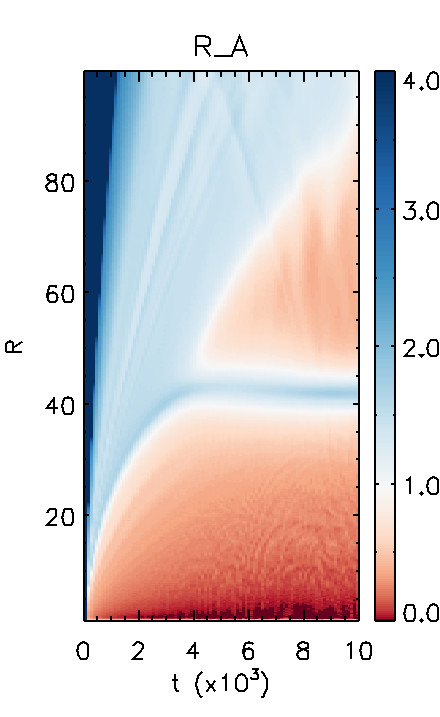
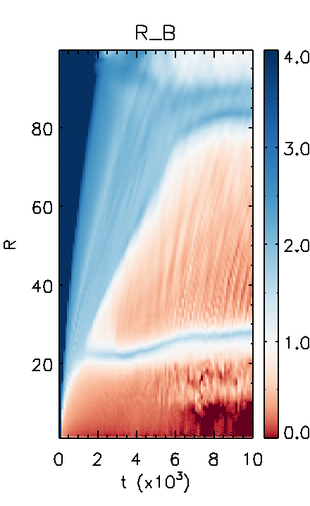
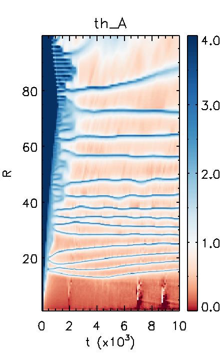
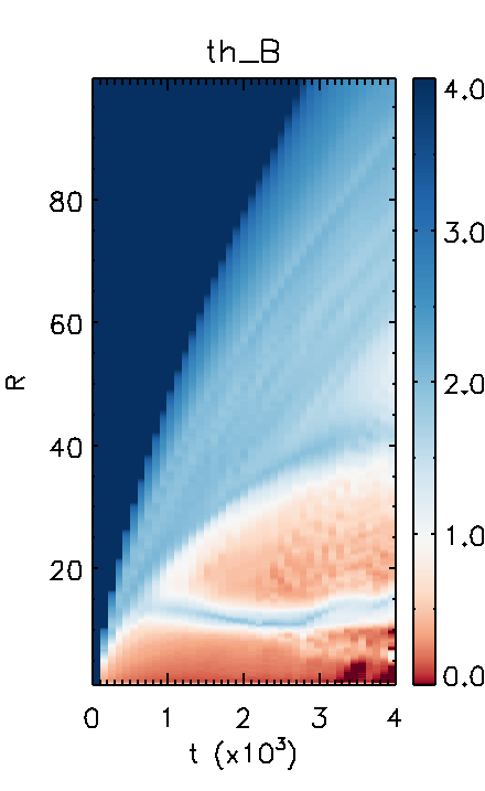
Figure 4: Dynamo number for selected simulation runs. Note the presentation of this figure as a t-R diagram, displaying the strength dynamo number along the disk (vertically, in R-direction) as a function of time (horizontal axis).

The dynamo number is usually quoted as a measure for dynamo activity. Only dynamos with a super-critical dynamo number evolve rapidly and work efficiently against magnetic diffusivity, and finally lead to a strong, saturated poloidal magnetic field. The dynamo number can therefore tell us when and where the growth of the magnetic field reaches saturation. In Figure 4 we compare the dynamo number as function of time and radius for different cases.

We first show the dynamo number for different strength of the tensor component $\alpha_{\phi}$ (top panel). We see that as $\chi$ decreases, the amplification of the poloidal field is weaker and also slower, as also indicated by Fig. 2. These differences in the magnetic field evolution are reflected on the dynamo number. In the time evolution of the dynamo number for all simulations we can clearly distinguish three evolutionary stages.

We may first define an (i) initial phase (indicated in blue) during which the dynamo number is almost infinite, simply because the diffusivity is still low (as implied by the quenching triggered by the magnetic diffusivity). Then comes a (ii) dynamo phase (indicated in white) that is characterized by a strong competition between dynamo action and diffusive quenching. During this phase we recognize magnetic loops being present, surviving from the early stages ($t\lesssim 500$ in the inner disk region) of dynamo evolution. In a subsequent (iii) final phase (indicated in red), these magnetic loops have been washed out or have been broken-up, respectively, and a quasi-steady state of the dynamo evolution is reached. The time scale when the final phase is reached depends of the radius (thus on the dynamical time scale that is defined by the disk rotation at this radius). In the inner radii the final stage is reached around $t\lesssim 500$, while in the outer disk regions is reached only at $t\gtrsim 5000$. In this final phase, dynamo action and diffusive quenching are fully balanced.

Note that in the inner disk region the second dynamo phase is missing because of the rapid evolution of the dynamo. Here, the magnetic energy reaches the saturation level already very early, with a timescale of the first two phases being much smaller.

Considering now the effect of different levels of dynamo an-isotropy we find the following results. For larger $\chi$ we do not find a second phase at larger radii since the magnetic field is amplified on a shorter timescale. In addition to that, for larger $\chi$ the first phase has a shorter lifetime at every radius.

Looking at the innermost parts of the accretion disk, a larger $\chi$ leads to an overall smaller dynamo number at the stage of quasi-steady state. This is a consequence of the quadratic dependence on the disk diffusivity (see Eq. 19) that balances, respectively quenches the mean-field dynamo effect. For the latest evolutionary stages we notice that, although this happens at different times, for each choice of $\chi$,the simulation reaches its steady stage also at a larger radius. This is an indicator of a faster evolution of the magnetic field for larger $\chi$.

Note that the dynamo number can also be used as a tracer to identify the dynamo-inefficient zones. As the latter correspond to a minimum in the magnetic diffusivity, here the dynamo number will have a sudden growth. On the other hand, the dynamo-inefficient zones are not only zones where the toroidal magnetic field has a minimum, but they also zones where the toroidal field cannot be amplified. For such reason, the general application of the dynamo number as a measure of dynamo activity can be misleading, since its sudden growth (in correspondence of the field reversal) does not necessarily lead to a further magnetic field amplification.

This is shown in Fig. 4, where we display in the bottom panels the dynamo number for the simulation runs that result in the generation of dynamo-inefficient zones. In contrast, the upper panels show simulations that do not lead to dynamo-inefficient zones. The figure nicely demonstrates a similar evolution of these simulation up to radii where the dynamo-inefficient zones have established when a quasi-steady state is reached.

Interestingly, the dynamo-inefficient zones – representing a minimum in the toroidal and in the radial magnetic field component, do not directly affect the dynamo activity further out. Outside the field reversal zone a saturation of the magnetic field can be reached. This is in particular visible when comparing the two right panels (runs phi_C and th_B).

Looking at the dynamo number in more detail, we understand why case R_A and case Scalar (isotropic dynamo) are almost not distinguishable (Fig. 2, left). The dynamo-inefficient zone that is present in the case R_A appears only at later stages of the evolution, as it is located at about $R\simeq 40$ while the magnetic field in the ambient parts of the disk is amplified only on a longer timescale. In contrary, the dynamo-inefficient zone of R_B is formed already earlier at $t\simeq 1000$, and therefore a different evolution of the poloidal disk magnetic field takes place, and also on a shorter timescale. The time evolution of cases th_A and th_B will be discussed below (see Section 3.4).

3.3 Dynamics of accretion-ejection

So far we have investigated mainly the evolution of the magnetic field structure that is generated by the accretion disk dynamo, applying different model assumptions for the dynamo tensor. Obviously, the difference in the field structure - difference in strength and geometry - will have strong impact on the dynamics of the accretion disk and the disk wind or jet. In this section we want to discuss the dynamical evolution of the accretion-ejection structure and compare the results for different dynamo models.

3.3.1 Accretion and ejection rate

As pointed in the previous sections, the dynamo tensor components that amplify the toroidal field ($\alpha_{R}$ and $\alpha_{\theta}$) work on longer timescales than the $\phi$-component of the dynamo tensor (which amplifies the poloidal magnetic field). Also, a larger dynamo component $\alpha_{\phi}$ leads to a higher magnetic diffusivity. In turn, this leads to a higher accretion rate, as shown in the top panel of Fig. 5, since the disk diffusivity enables to replenish the disk matter that is lost from the inner disk (by accretion or ejection) from the outer disk regions.

On the other hand, the ejection rate only weakly depends on the strength of the $\phi$-dynamo, especially in the early stages of the evolution, ($t\simeq 100$), as shown in the bottom panel of Fig. 5. While the inner regions reach a quasi-steady state for $t\gtrsim 500$, the ejection rate decreases until it reaches a quasi-constant level. This magnitude is higher for larger $\chi$, mostly because of the enhanced accretion rate.

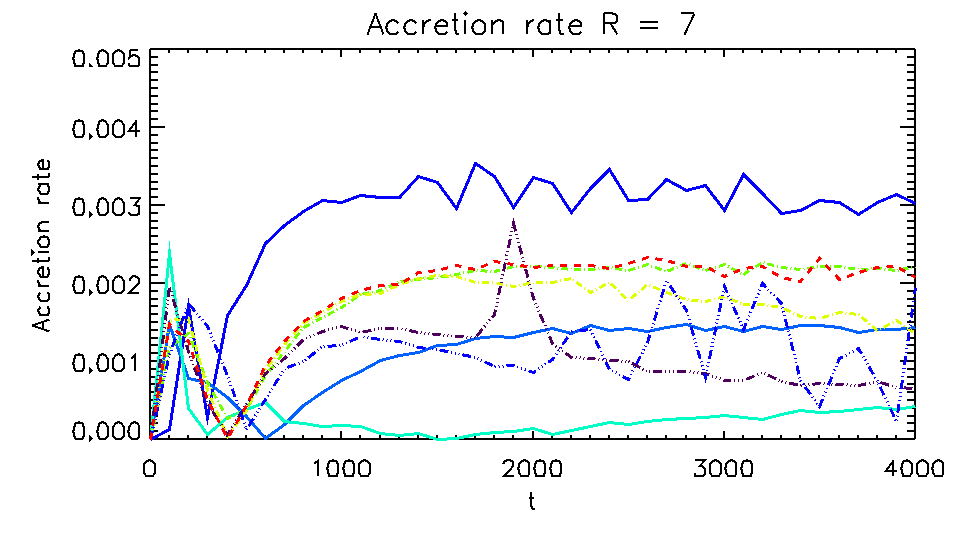
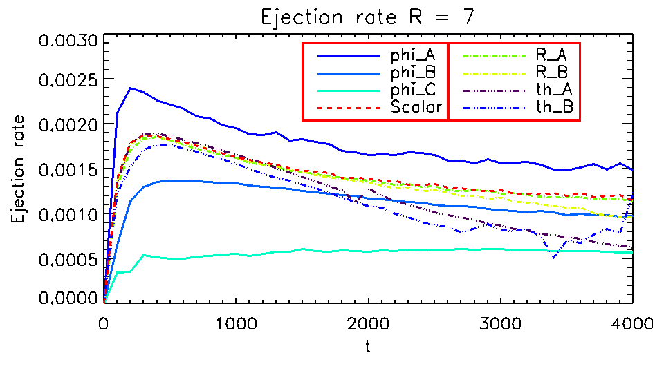
Figure 5: Temporal evolution of the accretion (top panel) and ejection (bottom panel) rates. The accretion rate is computed at fixed radius $R=7$, while the ejection rate is computed along the disk surface from $R=1$ to $R=7$. See Sect. B for a definition of the control volume.

We find that the ratio between the ejection and the accretion rate is higher for lower $\chi$. This can be understood as follows. A higher strength of $\alpha_{\phi}$ leads effectively to a stronger and faster amplification of the magnetic field. A larger $\chi$, which is itself a consequence of applying an anisotropic dynamo tensor, leads to a stronger disk magnetization. Because of the diffusive quenching we apply (see Eq. 19), a higher disk magnetization implies a higher disk magnetic diffusivity, which in turn supports higher accretion rates.

For example, Figure 5 shows that for $\chi=2.0$ about $<50\%$ with of the accretion mass flux becomes ejected. For $\chi<0.5$ all the matter accreted becomes ejected into the jet structure. This result is in nice agreement with resistive non-dynamo launching simulations (Zanni et al., 2007; Sheikhnezami et al., 2012), which showed a correlation between the disk magnetic diffusivity and the ejection-accretion rate ratio.

Once the poloidal field has become dynamo-amplified, the $R$ and $\theta$-components of the dynamo tensor can play a major role in the magnetic field evolution and, thus, also in the dynamics of accretion-ejection as they potentially induce dynamo-inefficient zones in the disk. For simulations for which NO dynamo-inefficient zones emerge, differences in the toroidal magnetic field do not really impact on the poloidal field components, even on longer time scales.

On the other hand we find that a toroidal field reversal and the subsequent formation of multiple anti-aligned loops (and the correspondent dynamo-inefficient zones) in the disk leads to a decrease in the accretion rate. The reason is the diffusive quenching we apply. At the locations where the toroidal field vanishes in the disk, also the magnetic diffusivity has a minimum (because of the low disk magnetization, see Eq. 19). A low diffusivity lowers the accretion efficiency.

We point out that the increase in the poloidal magnetic energy shown in Fig. 2 is a value integrated over a control volume. Therefore, even if the overall magnetic energy is high, the formation of zones of low magnetic diffusivity leads to a decrease in the overall accretion rate. As a consequence, the disk mass that is lost by accretion and ejection cannot be efficiently replenished, therefore the accretion rate decreases with time. Also the ejection rate is affected, but at later times. The most immediate consequence of the lower accretion rate is the formation of under-dense and over-dense zones in the accretion disk.

The radial distance of a dynamo-inefficient zone from the inner disk radius is strictly correlated with the timescale at which we observe a decrease in the accretion rate. This is the case for example for simulations R_B and R_A (see Fig. 5, left). While in the former case the dynamo-inefficient zone leads to a decrease in the accretion rate already at time $t\simeq 2000$, the latter case shows no difference to the simulation applying an isotropic dynamo tensor until time $t\simeq 4000$. Note that the dynamo-inefficient zone is formed only at $t\simeq 4000$, and, therefore, can impact the accretion and ejection rates only on a longer time scale (see Fig. 4).

3.3.2 Jet speed and collimation

An immediate consequence of a variation in the dynamo tensor components is the jet kinematics. As pointed by Stepanovs & Fendt (2016), a higher poloidal disk magnetization will leads to a stronger jet, for example in terms of mass flux and velocity. We know from simulations applying a scalar dynamo model (Fendt & Gaßmann, 2018) that the terminal jet speed is correlated with the strength of $\alpha_{0}$; in particular, a stronger dynamo leads to a faster jet. Note that these properties – jet speed, mass flux, or collimation – are global properties and thus accessible in principle by observations, different from the intrinsic local conditions in the disk such as turbulence and dynamo action.

As for the evolution of the magnetic field, the three components of the dynamo tensor have a different impact also for the jet kinematics. When considering different magnitudes of the dynamo-$\chi$, from our simulations we find an correlation similar to the one discovered in Stepanovs & Fendt (2016). That is the fact that a stronger $\phi-$component of the dynamo results in a stronger amplification of the poloidal magnetic field. As a direct consequence, since the midplane pressure shows only a very weak dependence on the dynamo model, a larger $\chi$ leads to a higher poloidal disk magnetization (see Fig. 6). Consequently, with a higher disk magnetization more magnetic energy is available to accelerate the outflow.

We show the terminal jet speed, here computed as the maximum speed at $R=100$, as function of the magnetization in Fig. 6. This figure indicates a very clear trend, as proposed by Stepanovs & Fendt (2016). In addition, it demonstrates again the gain in magnetization for different parameters for the dynamo parameter. We find that the maximum jet speed reaches the Keplerian velocity at the inner disk radius However, the maximum speed decreases for smaller $\chi$. This is shown also in Fig. 7 where we compare the distribution of the jet poloidal velocity for different simulation runs.

The two other dynamo tensor components affect the evolution of the disk magnetization in term of generation (or not generating) magnetic loops and/or dynamo-inefficient zones. Since minima in the magnetic field strength do only have a very minor impact on the overall disk poloidal magnetic energy (and therefore on the disk poloidal magnetization, see Fig. 5), a difference in $\phi$ does not necessarily lead to a different jet. The main reason why the jet dynamics is not substantially changed, at least in the early stages of the jet formation and propagation, is that the magnetic field structure remains very similar in the innermost disk regions (see Fig. 3). This is actually the field structure that is responsible for launching the strongest - and also collimated - jet component.

On the other hand, the dynamo-inefficient zones lead to a different disk mass distribution (see Fig. 5), which naturally affects the evolution of the whole disk-jet system. In particular, we observe a more turbulent configuration of the poloidal magnetic field (see Fig.7), which leads to the ejection of a slower and less massive jet (i.e. with smaller ejection rate, as shown in the bottom panel of Fig. 5). The latter has been proposed already by Fendt (2006).

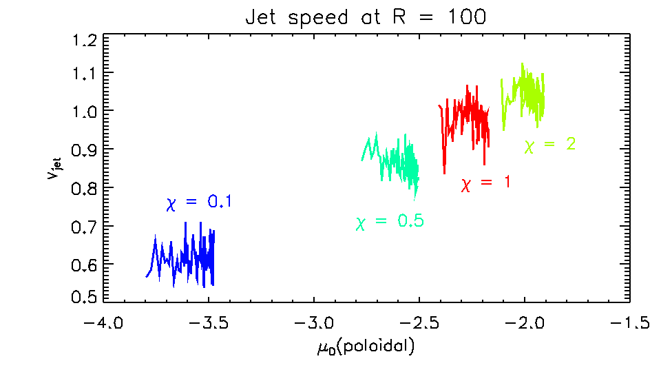
Figure 6: Jet speed vs disk magnetization. Shown is the maximum jet velocity versus the disk magnetization calculated from the poloidal magnetic field. Note that the disk magnetization is solely resolution from the dynamo component $xi$ and does not depend from a further quenching parameter.

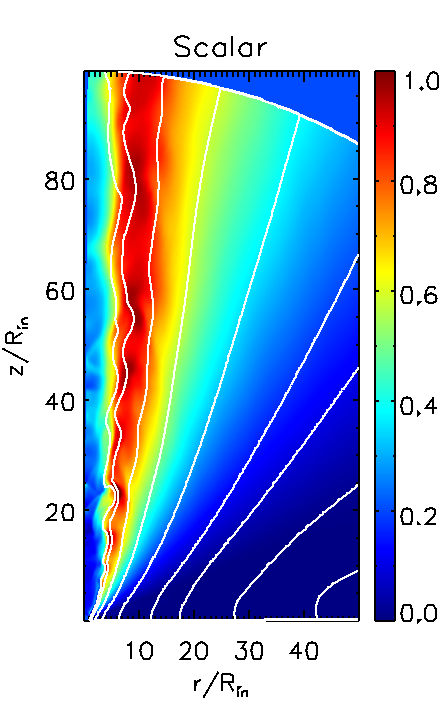
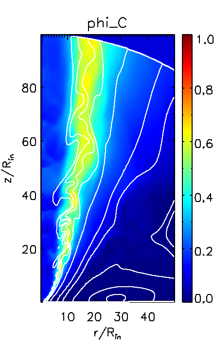
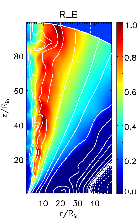
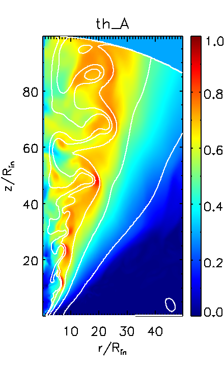
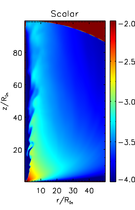
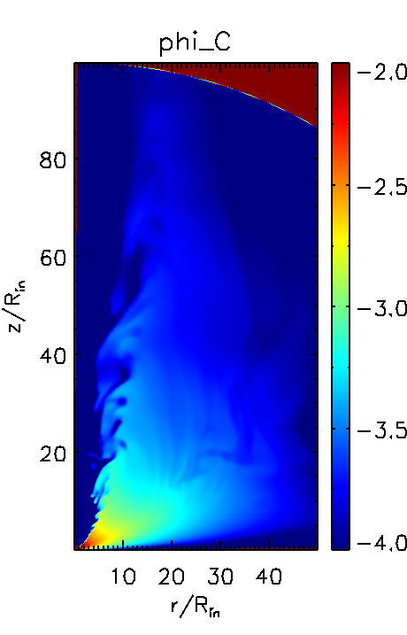
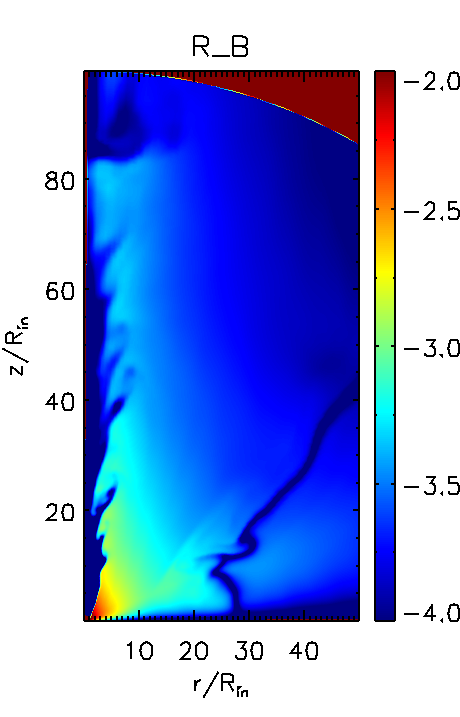
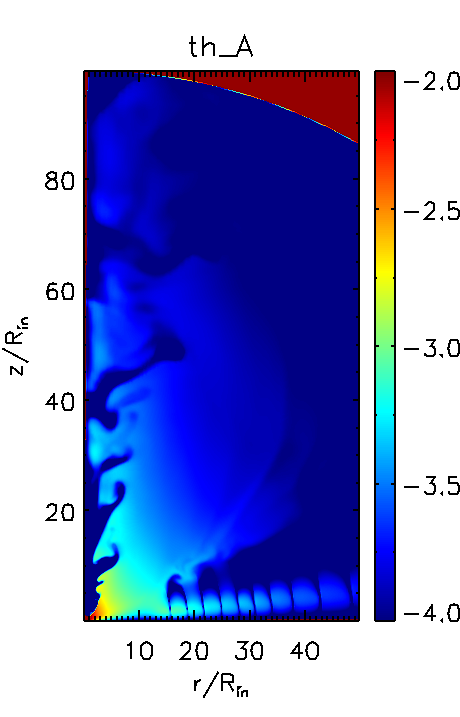
Figure 7: Comparison of parameter runs at $t=10000$. Shown is the distributions of the poloidal velocity (top), overlaid with contour lines of the vector potential (following poloidal field lines)(top), and toroidal magnetic field strength (bottom).

Another observable is the jet collimation as an imprint of the overall jet dynamics. There are several options how to best define jet collimation For example, in Fendt (2006); Pudritz et al. (2006); Sheikhnezami et al. (2012) the degree of collimation has been computed as the ratio of the (normalized) mass fluxes in the axial and in the lateral direction, respectively. Another option is the pure opening angle. Here we choose a different way to measure the jet collimation quantitatively, taking advantage of the spherical coordinates we applied. More specifically, we compute the opening angle of the jet flow for which the jet has its maximum velocity (or mass flux). Comparing the angle obtained for different (spherical) radii we obtain a gradual change that in particular demonstrates the process of collimation.

What we find from our dynamo simulations is essentially that the jet degree of collimation shows only a weak dependence on the strength of the dynamo component $\alpha_{\phi}$. This is maybe expected as we know that collimation depends on the profile of the disk magnetic field rather than its strength (Fendt, 2006; Pudritz et al., 2006). Therefore, no significant differences are found in the jet collimation for a substantially isotropic dynamo, while an anisotropic dynamo in general leads to a lower degree of jet collimation (see Fig. 7, left).

Another feature that impacts the degree of jet collimation is the presence of magnetic islands, respectively magnetized vortices. This loops severely disturb of the accretion-ejection structure, enhance the turbulence in the outflow flow, and also affect the efficiency of mass ejection.

The toroidal magnetic field, which plays a leading role in the jet collimation, is affected by $\alpha_{R}$ and $\alpha_{\theta}$. In particular, the existence of zones where the mean-field dynamo does not work efficiently, leads to a more turbulent configuration of both the poloidal and toroidal magnetic field (see Fig. 7, right). Note, however, that jets also self-generate a substantial toroidal field that usually supports collimation (Blandford & Payne, 1982). Here, the turbulent injection and the turbulent field structure hinder a regular jet toroidal field. Thus, a weak or non-isotropic dynamo will produce a less collimated jet (see again Fig. 7, right). To summarize, the dynamo-inefficient zones lead to a more turbulent evolution of both the magnetic field and the hydrodynamical quantities, resulting in a more turbulent and less collimated jet structure.

3.4 Early evolution

Since the target of this toy model is to investigate the effects of the different dynamo components on the launching process, we now discuss the impact of the tensor component $\alpha_{\theta}$ in more detail. This mostly relates to the very initial evolution of the simulation.

A first result is that for $0<\psi<3$ the evolution of the disk-jet system shows no difference when compared with a scalar dynamo. A likely explanation we find come directly from the choice of the initial configuration of the magnetic field in combination with the induction equation. Since the seed field is purely radial, there is no $B_{\theta}$-component that can be coupled by a dynamo process. Therefore, in the initial evolutionary states no contribution can be provided from $\alpha_{\theta}$. As the system evolves, the diffusive quenching takes place quite rapidly, leading to a quasi-steady state. Eventually, the dynamo effects are counterbalanced by magnetic diffusivity and the component $\alpha_{\theta}$ plays a minor role, just because they are weak and had no time to evolve.

However, when increasing $\alpha_{\theta}$, as for simulation run th_A, its dynamo effect on the temporal evolution becomes stronger. The most important difference to the scalar dynamo simulations is the formation of multiple dynamo-inefficient zones within the accretion disk. As the magnetic field can be amplified only between the dynamo-inefficient zones, this further leads to multiple regions in the disk where the magnetic diffusivity does not grow (see Fig. 4).

The reason why the early temporal evolution is mostly dominated by the other two dynamo components, essentially depends on the initial magnetic field configuration. On one hand this might look unphysical, as the long-term dynamo amplification of the magnetic field should not depend on its initial structure. On the other hand, a weak field seed must be present in order to initialize a mean-field dynamo effect.

Essentially, a toroidal initial magnetic field leads to the same results (see also Stepanovs et al. 2014). Similar to the case of a radial initial field, the component $\alpha_{\theta}$ is not involved in the initial temporal evolution of the $B_{\phi}$, and therefore is able to play a role only when the magnetic field has already saturated. Thus, the field evolution generated from a purely toroidal initial field leads to results similar to those obtained from a radial seed field.

This is in contrast to simulations starting from a vertical seed field. We find a strong impact on the evolution of the system because of the strong shear between the rotating disk and the non-rotating (at $t=0$) corona (Fendt & Gaßmann, 2018). In addition, this is amplified by the $\alpha_{\theta}$ dynamo effect of the magnetic field.

This can be nicely seen by our simulation th_B applying a vertical seed magnetic field that is derived from a constant vector potential $A_{\phi}=10^{-5}$ and is applying an anisotropic dynamo with $\psi=0.1$. Here, the vertical initial field is able to affect, through the mean-field dynamo, the magnetic field evolution and amplification. A dynamo-inefficient zone is formed around $R\simeq 15$. A collimated outflow is launched, although the overall jet structure shows less collimation compared to the simulation with isotropic dynamo (with radial initial field).

4 Conclusions

We have presented MHD dynamo simulations in the context of large-scale jet launching. Essentially, a magnetic field that is amplified by a mean-field disk dynamo, is able to drive a high speed jet. All simulations have been performed in axisymmetry, treating all three vector components for the magnetic field and velocity. We have applied the resistive code PLUTO 4.3 (Mignone et al., 2007), however extended by implementing an additional term in the induction equation that considers the mean-field dynamo action.

Extending our previous works on mean-field dynamo-driven jets (Stepanovs et al., 2014; Fendt & Gaßmann, 2018), here we have essentially investigated the effects of a non-scalar dynamo tensor. We have applied

(i) various (ad-hoc) choices for the dynamo tensor components (this paper, paper I), but also

(ii) an analytical model of turbulent dynamo theory (Rüdiger et al., 1995) that incorporates both the magnetic diffusivity and the turbulent dynamo term, connecting their module and anisotropy by only one parameter, the Coriolis number $\Omega^{*}$ (see paper II, Mattia & Fendt 2020).

In particular we have obtained the following results:

1) We have disentangled different effects of the dynamo tensor components concerning the magnetic field amplification and geometry. We find that the strength of the amplification is predominantly related to the dynamo component $\alpha_{\phi}$. The stability of the disk and the launching process can be affected by re-connection events. The field geometry that is favouring re-connection is mainly governed by the dynamo components $\alpha_{R}$ and $\alpha_{\theta}$.

2) We find that the component $\alpha_{\phi}$ is strongly correlated to the amplification of the poloidal magnetic field, such that a stronger $\alpha_{\phi}$ results in a more magnetized disk, which then launches a faster, more massive and more collimated jet. In contrast, the amplification of the poloidal field depends substantially on the existence of dynamo-inefficient zones, which, subsequently, affect the overall jet-disk evolution, thus accretion and ejection.

3) We find that not only a stronger dynamo component $\alpha_{\theta}$ but also a radial component $\alpha_{R}$ defined by $\phi<0.8\lor\phi>1.5$, respectively, leads to the formation of dynamo-inefficient zones. The formation of the dynamo-inefficient zones can also be triggered by a vertical component of the initial magnetic field, even for a weak dynamo component $\alpha_{\theta}$. A strong $\alpha_{\theta}$ component triggers the formation of the dynamo-inefficient zoned predominantly in the inner disk region. Those loops in general lead to a different evolution of the disk dynamics, since these zones are dynamo-inefficient and prevent accretion of material from the outer regions of the accretion disk to the inner disk that looses mass by accretion and ejection.

4) We have investigated how the action of the three different dynamo components affect the jet structure, respectively. We find the strength of the magnetic field has a minor influence on the jet speed and mass, however the field geometry, in particular the disk magnetic field profile matters a lot. For lower $\alpha_{\phi}$ or in presence of dynamo-inefficient zones within the accretion disk, the magnetic field follows a different configuration (with more large-scale magnetic compared a more turbulent structure), which immediately affects the jet structure and collimation.

5) We have disentangled a clear correlation between the anisotropy of the dynamo tensor and the large-scale motion of the jet. In particular, dynamos working with a larger $\alpha_{\phi}$ produce a magnetic field that is able to drive faster jets. The reason is that these dynamos lead to a stronger disk magnetization, thus provide more magnetic energy for launching. This result nicely couples to correlations between the disk magnetization and various parameters of the jet dynamics as found by Stepanovs & Fendt (2016).

6) We have investigated the formation of co-called dynamo-inefficient zones within the accretion disk and their effect on the disk-jet connection. In particular, such zones are related to a toroidal field reversal with zero derivative, which leads to the formation of multiple loops in the disk. As a consequence, the poloidal magnetic field (in both the disk and the jet) follows a more turbulent evolution, forming e.g. reconnecting magnetic loops, which affects the overall jet launching, the jet mass loading and, subsequently the jet propagation. These zones result from certain conditions for the dynamo action, i.e. certain combinations of the dynamo tensor components.

So far we have looked for non-isotropic dynamos applying (ad-hoc) choices for the dynamo tensor components. In our follow-up paper (paper II), we will apply an analytical model of turbulent dynamo theory (Rüdiger et al., 1995) that incorporates both the magnetic diffusivity and the turbulent dynamo term, connecting their module and anisotropy by only one parameter, the Coriolis number $\Omega^{*}$.

Appendix A Test simulations and comparison to the Literature

In order to validate our implementation of the mean-field dynamo tensor in the latest version of PLUTO, we have performed comparison simulations to the reference simulation of Fendt & Gaßmann (2018), now restricted to one hemisphere.

Note that while in Stepanovs et al. (2014); Fendt & Gaßmann (2018) the dynamo term was simply coupled with the magnetic diffusivity, here, because of its hyperbolic nature, the $\alpha$-tensor is coupled with the standard hyperbolic MHD flux terms, with a correction due to the solenoidal condition of the magnetic field. Some minor differences in the magnetic field evolution seem to arise from the different implementation schemes, however, the overall evolution of the system shows very small differences in the strength of the physical processes at work.

Our simulation runs till $t=30000$, corresponding to $\simeq 5000$ inner disk rotations. Figure 8 shows the evolution of the density and of the magnetic field lines. We may distinguish three different zones of evolution – the innermost disk, the outer disk, and the corona. The temporal evolution is in very good agreement with Fendt & Gaßmann (2018), evolving the same features.

Throughout the inner disk region the magnetic field lines have the typical open field lines inclined with respect to the disk surface. This configuration is particularly favorable for a Blandford-Payne-driven outflow. The outer disk region is filled with magnetic loops, which are pushed outwards by the magnetic pressure gradient and thereby diffusing through the disk until it is filled with magnetic energy and a local steady state is reached.

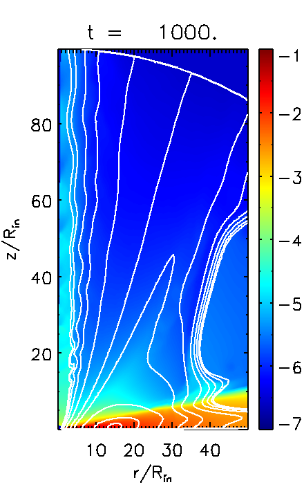
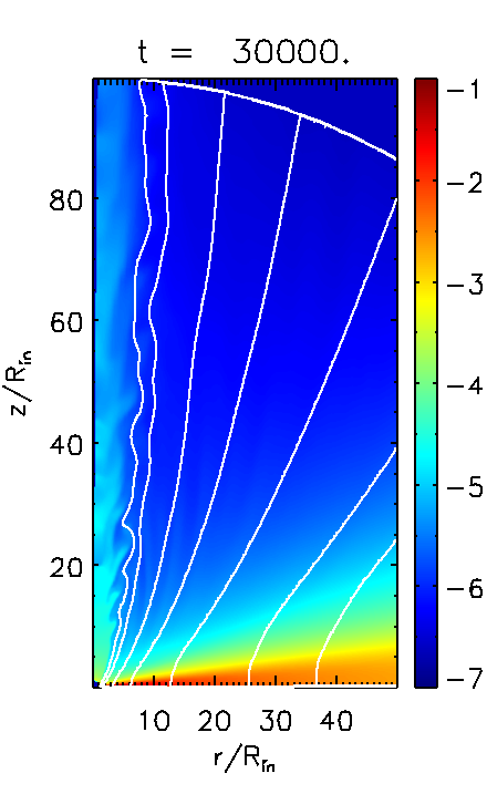
Figure 8: Comparison simulation. Snapshots at $t=[1000,30000]$ for a simulation with the the reference parameters of Fendt & Gaßmann (2018), now performed with PLUTO 4.3. The color map shows the density while the white lines are contours of the vector potential (poloidal magnetic field lines).

In difference to Fendt & Gaßmann (2018) we find that the poloidal magnetic energy saturates towards a somewhat level, but this is simply because our computational domain is smaller. Integrated over the whole disk Fendt & Gaßmann (2018) find a saturation magnitude of $\simeq 2\times 10^{-3}$ (in code units), while here we reach a saturation value of $\simeq 1.2\times 10^{-3}$ (assuming that the lower hemisphere follows the same evolution as the upper hemisphere).

On the other hand, the accretion and ejection rates saturate at similar magnitude, and also the accretion-ejection ratio agrees with our previous studies (Fendt & Gaßmann, 2018). This again strongly supports our conclusion that the different implementation schemes are identical.

A.1 The dynamo number

One way to examine the evolution of the dynamo action is to look at the time evolution of the dynamo number, Eq. 20. Dynamo quenching limits the dynamo number to a marginally sub-critical magnitude at which the alpha-dynamo is balanced by magnetic diffusivity. We point out that the critical dynamo number is not known a priori, but had to be derived from comparison of parameter studies. Furthermore, it tells us whether a particular disk region has reached a quasi-steady state. The evolution of the dynamo number is shown in Figure 9 as a function of time and radius, respectively.

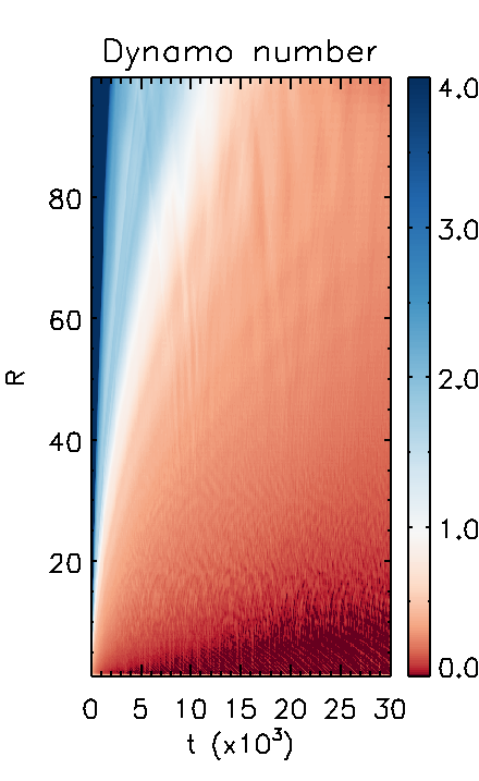
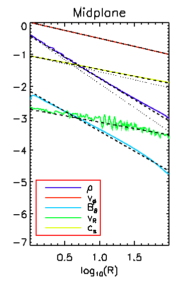
Figure 9: Comparison simulation. Evolution of the dynamo number and MHD variables for a simulation of with the the reference parameters of Stepanovs et al. (2014). Shown is the evolution of the dynamo number as a function of time and radius (left) over time, and the profile of certain physical quantities along the disk mid-plane (right) at $t=30000$. Colored lines indicate different physical quantities, $\rho$ (blue), $c_{\rm s}$ (yellow), $v_{\phi}$ (red), $B_{\theta}$ (cyan), and $v_{R}$ (green), while thin dashed lines show the initial power-law distribution. The thick dashed lines show the corresponding fit by a power-law.

At $t=0$ the dynamo number is almost infinite because of the weak magnetization, then it decreases starting from the inner radii and then reaching a quasi-steady state also in the outer regions. At $t=5000$ we can distinguish two areas in the profile of the dynamo number. For $R<60$, diffusive quenching has already lead to a field saturation. For larger radii the diffusivity still decreases as the toroidal magnetic field has not entirely engulfed the accretion disk.

At time $t=15000$ the dynamo-generated magnetic loops are diffused to large radii and the whole system has reached a stable configuration. For all radii the dynamo number is somewhat below 6, which we consider as the critical dynamo number for this simulation setup. We note that this magnitude is similar to what Brandenburg & Subramanian (2005) have suggested, although the critical dynamo number depends on the geometry and other physical details of the simulation setup. Going even further in time we see no difference in the temporal evolution nor in the dynamo number. Thus, all simulations were performed, if not specified otherwise, till $t=10000$.

A.2 Mid-plane quantities

Figure 9 shows the distribution of specific physical quantities along the disk mid-plane, measured at $t=30000$. This allows to compare our test simulations to the reference simulation of Stepanovs et al. (2014).

We have again fitted the simulation data points with a power law in order to extrapolate the power law index $\beta_{X}$ and compare it with the radial distribution at $t=0$. We find that the disk rotation remains Keplerian with $\beta_{v_{\phi}}=-1/2$. However, the radial profile of the density distribution changes substantially from $\beta_{\rho}=-3/2$ to $\beta_{\rho}=-4/3$ up to $R\simeq 30$, while for larger radii the power index is $\beta_{\rho}=-5/4$. As the total mass flux is conserved, the ejection of matter immediately changes the accretion rate over the disk and is thus related to the changes in the profiles of the mass fluxes. The radial (accretion) velocity follows a power law index $\beta_{v_{R}}=-2/5$. Since we are reaching a longer run time than Stepanovs et al. (2014), we are now able to get rid of the oscillations and also the reversal found by Stepanovs et al. (2014) in the outer disk regions (as their magnetic field was not yet diffused across the whole accretion disk).

The power-law coefficient of the sound speed changes during $t=0$ and $t=10000$ from $\beta_{\rm{cs}}=-1/2$ to $\beta_{\rm{cs}}=-3/7$, which tells us that the mean-field dynamo only slightly changes its strength as due to the disk sound speed through the disk-jet evolution (see Eq. 14). This change does not lead to any strong net effect on the temporal evolution of the disk-jet system, therefore we again find difference to our previous results (Stepanovs et al., 2014; Fendt & Gaßmann, 2018).

Also the angular magnetic field component $B_{\theta}$ follows the same power law, namely $\beta_{B_{\theta}}=-5/4$. Note, however, that we do not find the decrease in the outer disk regions ($R\geq 40$) as found in Stepanovs et al. (2014), simply because of our longer simulation time.

Overall, by quantifying essential dynamical properties of our simulation results, we find perfect agreement with the previous results that are based on a numerically different implementation of magnetic diffusivity and mean-field dynamo.

Appendix B Control volumes and fluxes

Here we define how we integrate global quantities that are used throughout the paper. The accretion rate is calculated by integrating the net radial mass flux through the disk, defined by an opening angle $\theta_{S}\equiv\arctan(2H/r)$,

$$\dot{M}_{\rm{acc}}(R)=2\pi R\int_{\pi/2}^{\pi/2-\theta_{S}}\rho v_{R}Rd\theta,$$ (B1)

while the ejection rate is calculated integrating the outflow in vertical direction (through the disk surface),

$$\dot{M}_{\rm{eje}}(R;\theta_{S})=\int_{R_{\rm{in}}}^{R}\rho v_{\theta}(\tilde{R})2\pi\tilde{R}d\tilde{R},$$ (B2)

respectively. The magnetic disk energy (poloidal or toroidal) is integrated from a radius of choice $R$ to the outer radius $R_{\rm{out}}$, and from the disk midplane to the disk surface, defined by $\theta_{S}$. We thus consider the disk magnetic energy outside $R$ for our considerations,

$$E_{\rm{mag}}=\int_{R}^{R_{\rm{out}}}\int_{\pi/2-\theta_{S}}^{\pi/2}\frac{1}{2}B^{2}\sin(|\theta|)2\pi R^{2}d\theta dR.$$ (B3)

The so-called disk magnetic field (and also the disk magnetization) is simply calculated as the average value of the magnetic field, at each radius, within the initial disk defined by $\theta_{i}\equiv\arctan(H/r)$,

$$B_{\rm{disk}}(R)=\displaystyle\frac{1}{\theta_{i}}\int_{\pi/2-\theta_{i}}^{\pi/2}B(R,\theta)d\theta\\$$ (B4)

while the so-called disk diffusivity is the average value of the diffusivity at a certain radius within the initial accretion disk,

$$\eta_{\rm{disk}}(R,t)=\frac{1}{\theta_{i}}\int_{\pi/2-\theta_{i}}^{\pi/2}\eta(R,\theta)d\theta$$ (B5)

References

- Bai & Stone (2013) Bai, X.-N. & Stone, J. M. 2013, ApJ, 767, 30
- Balbus & Hawley (1991) Balbus, S. A. & Hawley, J. F. 1991, ApJ, 376, 214
- Bardou et al. (2001) Bardou, A., von Rekowski, B., Dobler, W., Brandenburg, A. & Shukurov, A. 2001, A&A, 370, 635
- Blandford & Payne (1982) Blandford, R. D. & Payne, D. G. 1982, MNRAS, 199, 883
- Brandenburg & Subramanian (2005) Brandenburg, A. & Subramanian, K. 2005, Phys. Rep., 417, 1
- Brandenburg et al. (1995) Brandenburg, A., Nordlund, A., Stein, R. F. & Torkelsson, U. 1995 ApJ, 446, 741
- Bucciantini & Del Zanna (2013) Bucciantini, N., & Del Zanna, L. 2013, MNRAS, 428, 71
- Bugli et al. (2014) Bugli, M., Del Zanna, L., & Bucciantini, N. 2014, MNRAS, 440, L41
- Campbell (1999) Campbell, C. G. 1999, MNRAS, 310, 1175
- Campbell (2009) Campbell, C. G. 2009, MNRAS, 392, 271
- Casse & Ferreira (2000a) Casse, F. & Ferreira, J. 2000a, A&A, 353, 1115
- Casse, & Ferreira (2000b) Casse, F., & Ferreira, J. 2000b, A&A, 361, 1178
- Casse & Keppens (2002) Casse, F. & Keppens, R. 2002, ApJ, 581, 988
- Chabrier & Küker (2006) Chabrier, G., & Küker, M. 2006, A&A, 446, 1027
- Dhang et al. (2020) Dhang, P., Bendre, A., Sharma, P., Subramanian, K. 2020, MNRAS, 494, 4854
- Dyda et al. (2018) Dyda, S., Lovelace, R. V. E., Ustyugova, G. V., et al. 2018, MNRAS, 477, 127
- Fendt (2006) Fendt, C. 2006, ApJ, 651, 272
- Fendt & Gaßmann (2018) Fendt, C., & Gaßmann, D. 2018, ApJ, 855, 130
- Ferreira & Pelletier (1995) Ferreira, J. & Pelletier, G. 1995, A&A, 295, 807
- Fleming et al. (2000) Fleming, T. P., Stone, J. M., & Hawley, J. F. 2000, ApJ, 530, 464
- Fleming & Stone (2003) Fleming, T. P., Stone, J. M. 2003, ApJ, 585, 908
- Flock et al. (2012) Flock, M., Henning, T., & Klahr, H. 2012, ApJ, 761, 95
- Frank et al. (2014) Frank, A., Ray, T. P., Cabrit, S., et al. ”Jets and Outflows from Star to Cloud: Observations Confront Theory”, in H.Beuther et‘al. (eds), Protostars and Planets VI, University of Arizona Press (2014)
- Fromang et al. (2002) Fromang, S., Terquem, C., Balbus, S.A. 2002, MNRAS, 329, 18
- Gammie (1996) Gammie, C. F. 1996, ApJ, 457, 355
- Gressel (2010) Gressel, O. 2010, MNRAS, 405, 41
- Gressel & Pessah (2015) Gressel, O., & Pessah, M. E. 2015, ApJ, 810, 59
- Hawley et al. (2015) Hawley, J. F., Fendt, C., Hardcastle, M., Nokhrina, E. & Tchekhovskoy, A. 2015, Space Sci. Rev.191, 441
- Hogg & Reynolds (2018) Hogg, J. D. & Reynolds, C. S. 2018, ApJ, 861, 24
- Jacquemin-Ide et al. (2019) Jacquemin-Ide, J., Ferreira, J., & Lesur, G. 2019, MNRAS, 490, 3112
- King et al. (2007) King, A. R., Pringle, J. E., & Livio, M. 2007, MNRAS, 376, 1740
- Krasnopolsky et al. (1999) Krasnopolsky, R. and Li, Z.-Y. and Blandford, R. 1999, ApJ, 526, 631
- Krause & Rädler (1980) Krause, F. &Rädler, K.-H. (eds), Mean-field magnetohydrodynamics and dynamo theory, Oxford, Pergamon Press, Ltd, 1980
- Londrillo & del Zanna (2004) Londrillo, P., & del Zanna, L. 2004, Journal of Computational Physics, 195, 17
- Mattia & Fendt (2020) Mattia, G. & Fendt, C. 2020, ApJ, revised (paper II)
- Mignone et al. (2007) Mignone, A., Bodo, G., Massaglia, S., Matsakos, T., Tesileanu, O., Zanni, C., & Ferrari, A. 2007, ApJS, 170, 228
- Mignone (2014) Mignone A., 2014, JCoPh, 270, 784
- Murphy et al. (2010) Murphy, G. C., Ferreira, J. & Zanni, C. 2010, A&A, 512, A82
- Ouyed & Pudritz (1997) Ouyed, R., & Pudritz, R. E. 1997, ApJ, 482, 712
- Pelletier & Pudritz (1992) Pelletier, G., & Pudritz, R. E. 1992, ApJ, 394, 117
- Pinilla et al. (2016) Pinilla, P., Flock, M., Ovelar, M. de J., et al. 2016, A&A, 596, A81
- Pudritz (1981a) Pudritz, R. E. 1981a, MNRAS, 195, 881-914
- Pudritz (1981b) Pudritz, R. E. 1981b, MNRAS, 195, 897
- Pudritz et al. (2006) Pudritz, R.E., Rogers, C.S., Ouyed, R. 2006, MNRAS, 365, 1131
- Pudritz & Ray (2019) Pudritz, Ralph E. & Ray, Tom P. 2019, Frontiers in Astronomy and Space Sciences, 6, 54
- Rincon (2019) Rincon, F. 2019, Journal of Plasma Physics, 85, 205850401
- Riols, & Latter (2018) Riols, A. & Latter, H. 2018, MNRAS, 474, 2212
- Rüdiger, & Kichatinov (1993) Rüdiger, G., & Kichatinov, L. L. 1993, A&A, 269, 581
- Rüdiger et al. (1995) Rüdiger, G., Elstner, D. & Stepinski, T.F. 1995, A&A, 298, 934
- Sano et al. (2000) Sano, T., Miyama, S.M., Umebayashi, T. 2000, ApJ, 543, 486
- Shakura & Sunyaev (1973) Shakura, N. I. & Sunyaev, R. A. 1973, A&A, 24, 337
- Sheikhnezami et al. (2012) Sheikhnezami, S., Fendt, C., Porth, O., Vaidya, B., & Ghanbari, J. 2012, ApJ, 757, 65
- Stepanovs & Fendt (2014) Stepanovs, D. & Fendt, C. 2014, ApJ, 793, 31
- Stepanovs et al. (2014) Stepanovs, D., Fendt, C. & Sheikhnezami, S. 2014, ApJ, 796, 29
- Stepanovs & Fendt (2016) Stepanovs, D. & Fendt, C. 2016, ApJ, 825, 14
- Stepinski & Levy (1988) Stepinski, T. F., & Levy, E. H. 1988, ApJ, 331, 416
- Stepinski & Levy (1990) Stepinski, T. F., & Levy, E. H. 1990, ApJ, 362, 318
- Tomei et al. (2020) Tomei, N., Del Zanna, L., Bugli, M., et al. 2020, MNRAS, 491, 2346
- Torkelsson & Brandenburg (1994) Torkelsson, U., & Brandenburg, A. 1994, A&A, 283, 677
- Toro (2009) Toro, E.F., Riemann Solvers and Numerical Methods for Fluid Dynamics: A Practical Introduction
- Tzeferacos et al. (2009) Tzeferacos, P. Ferrari, A. Mignone, A. Zanni, C. Bodo, G. & Massaglia, S. 2009, MNRAS, 400, 820
- Tzeferacos et al. (2013) Tzeferacos P., Ferrari A., Mignone A., Zanni C., Bodo G., Massaglia S., 2013, MNRAS, 428, 3151
- Uchida & Shibata (1985) Uchida, Y., & Shibata, K. 1985, PASJ, 37, 515
- von Rekowski et al. (2000) Rekowski, M. v., Rüdiger, G. & Elstner, D. 2000, A&A, 353, 813-822
- von Rekowski et al. (2003) von Rekowski, B., Brandenburg, A., Dobler, W., Dobler, W. & Shukurov, A. 2003, A&A, 398, 825
- von Rekowski & Brandenburg (2004) von Rekowski, B. & Brandenburg, A. 2004, A&A, 420, 17
- Vourellis & Fendt (2020) Vourellis, C. & Fendt, C. 2020, submitted
- Zanni et al. (2007) Zanni, C., Ferrari, A., Rosner, R., Bodo, G., & Massaglia, S. 2007, A&A, 469, 811