Updated predictions for gravitational waves produced in a strongly supercooled phase transition

Abstract

We update predictions for the gravitational wave (GW) signal from a strongly supercooled phase transition in an illustrative classically conformal U(1)_B-L model. We implement $\propto\gamma^{2}$ scaling of the friction on the bubble wall and update the estimates for the efficiency factors for GW production from bubble collisions and plasma-related sources. We take into account the fact that a small decay rate of the symmetry-breaking field may lead to brief matter-dominated era after the transition, as the field oscillates around its minimum before decaying. We find that a strong bubble collision signal occurs in a significant part of the parameter space, and that the modified redshift of the modes that re-enter the horizon during the matter-dominated period generates a characteristic tilted ‘plateau’ in the spectrum. The GW spectrum in this model would be detectable in the low-frequency range, e.g., by LISA, and in the mid-frequency range, e.g., by AION/MAGIS and AEDGE, and in the high-frequency range by LIGO and ET. The peak frequency of the signal is limited from below by collider constraints on the mass of the U(1)_B-L gauge boson, while at high frequencies the slow decay of the scalar field and the resulting matter-dominated era diminishes the GW signal.

1 Introduction

The electroweak phase transition is not predicted to be first order within the Standard Model (SM). However, a first-order phase transition is a common feature in many extensions of the SM, including models with higher-dimensional multi-Higgs interactions, additional scalar fields and extended gauge groups. Historically, the possibility of a first-order phase transition attracted interest because it facilitated electroweak baryogenesis [1, 2, 3, 4]. However, the direct detection of gravitational waves (GWs) by the LIGO and Virgo Collaborations [5] has recently stimulated widespread interest in the potential observability of GWs [6] produced in such a transition [7, 8, 9, 10, 11, 12, 13, 14, 15, 16, 17, 18, 19, 20, 21, 22, 23, 24, 25, 26, 27, 28, 29, 30, 31, 32, 33, 34, 35, 36, 37, 38, 39, 40, 41, 42, 43, 44, 45, 46, 47]. Another interesting possibility is that a first-order phase transition may have played a role in the generation of an intergalactic magnetic field [48, 49, 50, 51].

A primary ingredient in the calculation of the GW spectrum arising from a first-order phase transition is the calculation of the velocities of walls of bubbles of the true vacuum. Over the years many groups have contributed to the progress in this notoriously difficult calculation [52, 53, 54, 55, 56, 57, 58, 59]. In particular, there has recently been a significant advance in the estimation of the scaling of the friction, $P$, encountered by the wall with its Lorentz factor, with the result that $P\propto\gamma^{2}$ [59], to be contrasted with the previous estimate [56] that $P\propto\gamma$.

This change in the scaling law has a crucial impact on the amount of energy that is transferred into the plasma instead of the scalar field gradients, which tends to reduce the importance of bubble wall collisions as a source of GWs [60]. However, we show here that this modification does not necessarily change qualitatively the GW predictions found previously in models featuring a very strong first-order phase transition. To illustrate this point, we revisit the classically conformal $U(1)_{B-L}$ extension of the SM [12, 23, 35, 60], and show that there is no dramatic change in the regions of the parameter space where a strong GW signal from bubble collisions is predicted.

Also, we highlight a feature in the GW spectrum that can appear in many models predicting such a strong transition. As the strength of the transition increases, the decay width of the field involved decreases and, as a result, the reheating after the transition is not necessarily instantaneous. It can instead be preceded by a period during which the field oscillates around its minimum, effectively as during a matter-dominated epoch [61]. This period is reflected in the GW spectrum, because it modifies the redshifting history [62]. This effect produces a characteristic tilted plateau-like feature in the part of the spectrum due to super-horizon modes, which could in principle be used by GW detectors to probe the field decay rate directly.

The structure of this paper is as follows. In Section 2 we review the classically conformal ${\rm U}(1)_{B-L}$ model that we study, and in Section 3 we discuss the phase transition in this model, delineating in Fig. 1 the region where this transition is strongly first-order. Then, in Section 4 we consider the Lorentz factor of the bubble wall, commenting that the bubbles collide before they reach terminal velocity in much of the region where the transition is strong, and updating the estimate for the efficiency factor for GW production from bubble collisions. In Section 5 we present the calculation of the GW signal and in Section 6 we consider the impact on the signal of a matter-dominated period, displaying the plateau feature that is a signal of the slow decay of the ${\rm U}(1)_{B-L}$-breaking scalar field. Finally, in Section 7 we discuss the observability of the GW signal from the phase transition by LIGO [63, 64, 65] and the future GW detectors LISA [66, 67], AION [68], MAGIS [69, 70], AEDGE [71] and the Einstein Telescope (ET) [72, 73], as summarised in Fig. 7. Finally Section 8 summarises our results and discusses their implications.

2 Classically conformal ${\rm U(1)}_{B-L}$ model

Following Ref. [35], we describe briefly the scalar potential and the symmetry-breaking pattern in a classically conformal ${\rm U}(1)_{B-L}$ extension of the SM [74]. In addition to the SM particle content, this model includes the ${\rm U}(1)_{B-L}$ gauge boson $Z^{\prime}$, three right-handed neutrinos that cancel the ${\rm U}(1)_{B-L}$ anomaly, and a complex scalar $\phi=(\varphi+iG)/\sqrt{2}$ with $B-L$ charge $+2$, responsible for the breaking of the ${\rm U}(1)_{B-L}$ symmetry in vacuum. At tree level, the scalar potential of this model is

$$V=\lambda_{H}(H^{\dagger}H)^{2}+\lambda_{\phi}(\phi^{\dagger}\phi)^{2}-\lambda_{p}(H^{\dagger}H)(\phi^{\dagger}\phi)\,,$$ (2.1)

where $H$ is the Higgs doublet and $\lambda_{H},\lambda_{\phi},\lambda_{p}>0$.

For values of the $B-L$ gauge coupling $g_{B-L}\sim 0.1$, collider searches give a lower bound for the $B-L$ gauge boson mass: $m_{Z^{\prime}}\mathrel{\raise 1.29167pt\hbox{$>$\kern-7.5pt\lower 4.30554pt\hbox{$\sim$}}}4$ TeV [75, 76]. This can be converted into a lower bound on the $\varphi$ vacuum expectation value $\langle\varphi\rangle=w$ though $m_{Z^{\prime}}=2g_{B-L}w$, giving $w>\mathcal{O}(1\,{\rm TeV})\gg v\approx 246\,$GeV. In this case the symmetry breaking occurs first along the $\varphi$ direction. The one-loop effective potential  along this direction is given by

$$V_{\rm eff}=\frac{\lambda_{\phi}(t)}{4}\varphi^{4}+\frac{T^{4}}{2\pi^{2}}\sum_{j}k_{j}J_{T}\left(m_{j}(\varphi)^{2}+\Pi_{j}(T)\right)\,.$$ (2.2)

The first term in Eq. (2.2) is the $T=0$ one-loop renormalisation-group (RG)-improved scalar potential with the RG scale chosen to $t=\log(\varphi/\mu_{0})$, where $\mu_{0}$ is a reference scale for which we take the top quark mass $\mu_{0}=173\,$GeV. The second term accounts for one-loop finite-temperature effects. The sum over $j$ includes the $B-L$ gauge boson, the right-handed neutrinos, the scalar boson $\varphi$ and the Goldstone boson $G$, and the factors $k_{j}$ are their numbers of intrinsic degrees of freedom. The field-dependent masses for the U$(1)_{B-L}$ gauge boson $Z^{\prime}$, the right-handed neutrinos ($i=1,2,3$), the scalar boson $\varphi$ and the Goldstone boson $G$ are given by

$$m_{Z^{\prime}}(\varphi)^{2}=4g_{B-L}(t)^{2}\varphi^{2}\,\quad M_{i}(\varphi)^{2}=Y_{i}(t)^{2}\varphi^{2}/2\,,$$ (2.3)

$$m_{\varphi}(\varphi)^{2}=3\lambda_{\phi}(t)\varphi^{2}\,,\quad m_{G}(\varphi)^{2}=\lambda_{\phi}(t)\varphi^{2}\,,$$

and their Debye masses are

$$\Pi_{Z^{\prime}}(T)=4g_{B-L}(t)^{2}T^{2}\,,$$ (2.4)

$$\Pi_{\varphi}(T)=\frac{T^{2}}{24}\left[24g_{B-L}(t)^{2}+8\lambda_{\phi}(t)+\sum_{i}Y_{i}(t)^{2}\right]\,,$$

$$\Pi_{G}(T)=\Pi_{\varphi}(T)\,.$$

The Yukawa couplings of the right-handed neutrinos to $\phi$ are denoted by $Y_{i}$. The thermal integral $J_{T}$ is defined as

$$J_{T}(x)=\int_{0}^{\infty}{\rm d}y\,y^{2}\ln\left[1\mp e^{-\sqrt{x+y^{2}}}\right]\,,$$ (2.5)

with the negative sign for bosons and the positive sign for fermions.

The vacuum expectation value of $\varphi$ induces a negative mass term for the Higgs field, and the electroweak symmetry breaks in the same way as in the SM. However, if the $B-L$ breaking is delayed to temperatures below the QCD scale, the QCD phase transition happens first, inducing a linear term for the Higgs field, $\sum_{j}y_{j}\langle\psi_{j}\bar{\psi}_{j}\rangle h/\sqrt{2}$. The Higgs field then acquires a small non-zero expectation value. Therefore, for $T<T_{\rm QCD}$ the effective potential along the $\varphi$ direction becomes

$$V_{\rm eff}(T<T_{\rm QCD})=-\frac{\lambda_{p}(t)v_{\rm QCD}^{2}}{4}\varphi^{2}+V_{\rm eff}(T>T_{\rm QCD})\,,$$ (2.6)

where $v_{\rm QCD}\simeq 0.1\,$GeV. After the transition the QCD and electroweak symmetries are restored as the decay of the vacuum energy reheats the plasma, and, again, the evolution proceeds as in the SM. In the following we focus on the U$(1)_{B-L}$-breaking phase transition.

The model also includes kinetic mixing between the ${\rm U}(1)_{B-L}$ and hypercharge ${\rm U}(1)_{Y}$ gauge symmetries. The kinetic mixing term can be removed by a rotation and a rescaling of the gauge fields. After this the ${\rm U}(1)_{B-L}\times{\rm U}(1)_{Y}$ part of the covariant derivative is given by

$$\mathcal{D}_{\mu}\supset ig_{Y}q_{Y}B_{Y}^{\mu}+i(\tilde{g}q_{Y}+g_{B-L}q_{B-L})B_{B-L}^{\mu}\,,$$ (2.7)

where the coupling $\tilde{g}$ parametrizes the kinetic mixing, $q_{j}$ denotes the charges, $g_{j}$ the gauge couplings and $B_{j}^{\mu}$ the gauge fields. For $w\gg v$ and $g_{B-L}\sim 0.1$ the effect of the kinetic mixing on the $Z^{\prime}$ mass can be neglected and also the mixing angle between $Z$ and $Z^{\prime}$ gauge bosons is tiny (see e.g. Ref. [79]). The kinetic mixing affects the running of the Higgs quartic coupling and can stabilize the electroweak vacuum. In the following we fix $\tilde{g}=-0.5$ at $t=\log(w/\mu_{0})$, which was shown in Ref. [35] to keep $\lambda_{h}$ positive while retaining the perturbativity of the couplings up to the Planck scale for $g_{B-L}\mathrel{\raise 1.29167pt\hbox{$<$\kern-7.5pt\lower 4.30554pt\hbox{$\sim$}}}0.42$. The phase transition dynamics, however, is not very sensitive to the value of $\tilde{g}$, which enters the one-loop effective potential only through the running of $g_{B-L}$.

We assume that the Majorana Yukawa couplings of the right-handed neutrinos can be neglected, $Y_{i}\ll g_{B-L}$. We fix the couplings $\lambda_{\phi}$ and $\lambda_{p}$ and at $t=\log(w/\mu_{0})$ so that ${\rm d}V/{\rm d}\varphi=0$ at $\varphi=w$ and $\lambda_{p}=v^{2}/w^{2}$. The remaining free parameters are then the gauge coupling $g_{B-L}$ and the vacuum expectation value $w$, which we trade for the $Z^{\prime}$ mass, $m_{Z^{\prime}}=2g_{B-L}w$. In the following we show the results as a function of these two parameters, with the chosen value of $g_{B-L}$ corresponding to the scale $t=\log(w/\mu_{0})$.

3 Phase transition

We compute the details of the phase transition in a standard way, starting from the decay rate of the false vacuum due to thermal fluctuations [80]:

$$\Gamma(T)\simeq T^{4}\left(\frac{S_{3}}{2\pi T}\right)^{\frac{3}{2}}e^{-S_{3}/T}\,,$$ (3.1)

where the action of the O$(3)$ symmetric field configuration is

$$S_{3}=4\pi\int r^{2}{\rm d}r\left[\frac{1}{2}\left(\frac{{\rm d}\varphi}{{\rm d}r}\right)^{2}+V_{\rm eff}(\varphi,T)\right]\,.$$ (3.2)

The decay is dominated by the classical path that is the solution of the equation of motion obtained from the above action,

$$\frac{{\rm d}^{2}\varphi}{{\rm d}r^{2}}+\frac{2}{r}\frac{{\rm d}\varphi}{{\rm d}r}=\frac{{\rm d}V_{\rm eff}}{{\rm d}\varphi}\,,$$ (3.3)

with boundary conditions ${\rm d}\varphi/{\rm d}r=0$ at $r=0$ for the solution to be regular at the bubble centre, and $\varphi\to 0$ at $r\to\infty$ to describe the initial false vacuum background far from the bubble.

As shown in Ref. [81], taking particular care of the subsequent evolution of bubbles is crucial for very strong transitions. The probability that a given point remains in the unstable vacuum is given by $P=e^{-I(T)}$, where [82, 83]

$$I(T)=\frac{4\pi}{3}\int_{T}^{T_{c}}\frac{{\rm d}T^{\prime}\,\Gamma(T^{\prime})}{T^{\prime 4}H(T^{\prime})}\left(\int_{T}^{T^{\prime}}\frac{{\rm d}\tilde{T}}{H(\tilde{T})}\right)^{3}\,.$$ (3.4)

To find the percolation temperature, $T_{*}$, we solve for the condition $I(T_{*})=0.34$ [81], while ensuring that the volume of the false vacuum is decreasing:

$$\frac{1}{V_{\rm false}}\frac{dV_{\rm false}}{dt}=H(T)\left(3-T\frac{dI(T)}{dT}\right)<0\,,$$ (3.5)

so as to verify that percolation is possible despite the exponential expansion of the false vacuum.

The parameters relevant for the GW signal are then evaluated at $T=T_{*}$. These are the strength of the transition [84, 85],

$$\alpha\equiv\frac{1}{\rho_{R}}\left(\Delta V-\frac{T}{4}\Delta\frac{{\rm d}V}{{\rm d}T}\right)\bigg{|}_{T=T_{*}}\simeq\frac{\Delta V}{\rho_{R}(T_{*})}\,,$$ (3.6)

and the characteristic length scale for the transition given by the average bubble radius [86, 87],

$$R_{*}=\left[T_{*}\int_{T_{*}}^{T_{c}}\frac{{\rm d}T^{\prime}}{T^{\prime 2}}\frac{\Gamma(T^{\prime})}{H(T^{\prime})}e^{-I(T^{\prime})}\right]^{-\frac{1}{3}}\,,$$ (3.7)

which can be translated into the more commonly used time scale using $\beta=(8\pi)^{\frac{1}{3}}/R_{*}$ for strong transitions.

After the phase transition the scalar field oscillates around the true vacuum and decays heating the plasma. The decay of $\varphi$ is dominated by decays to two Higgs bosons, $\varphi\to hh$, and the decay width can be approximated as

$$\Gamma_{\varphi}\approx\frac{\lambda_{p}^{2}v_{\varphi}^{2}}{32\pi m_{\varphi}}\approx 2.5\times 10^{7}g_{B-L}\left(\frac{m_{Z^{\prime}}}{\rm GeV}\right)^{-3}\,,$$ (3.8)

where we have used $m_{\varphi}\approx 0.4g_{B-L}m_{Z^{\prime}}$ [35]. We discuss the possible matter-dominated period caused by slow decay of $\varphi$ and a suitably accurate prescription for the calculation of redshifting of the GW spectrum in this scenario in Section 6.

We display the phase transition parameters obtained in the classically conformal U$(1)_{B-L}$ model in Fig. 1, focusing on the region of parameter space where $\alpha>1$. We see that, in general, the percolation temperature $T_{*}$ (left panel) decreases and the strength of the transition $\alpha$ (middle panel) increases for smaller values of the gauge coupling $g_{B-L}$. However, the trend in $\alpha$ changes when $T_{*}<T_{\rm QCD}$, at which point the transition is catalysed by quark condensation and the transition cannot become any stronger. For $T_{*}<T_{\rm QCD}$ the strength of the transition is determined by $m_{Z^{\prime}}$. The average size of the bubbles at collision $R_{*}$ (right panel) is maximised compared to the horizon size when $g_{B-L}\simeq 0.25$, becoming slightly smaller for larger $g_{B-L}$ and significantly smaller for smaller $g_{B-L}$. We have cut off the lower right corners of the planes as there our assumption that $R_{*}$ is much bigger than the initial bubble radius does not hold (see Fig. 2).

Figure 1: A selection of $(m_{Z^{\prime}},g_{B-L})$ planes, colour-coded according to the percolation temperature, $T_{*}$ (left), the strength of the transition, $\alpha$ (middle) and the average bubble radius at collisions, $R_{*}$ (right). Below the dotted curve $\alpha>1$, below the dashed curve $T_{*}<T_{\rm QCD}$, to the right of the dot-dashed curve $\Gamma_{\phi}<H_{*}$, and below the solid curve the bubbles collide before they reach terminal velocity (See Fig. 2). The region to the left of the gray line is excluded by collider searches.

The main modification due to the increase in $m_{Z^{\prime}}$ is an increase in the vacuum energy difference, which we find to be related to the $Z^{\prime}$ mass by

$$\Delta V\approx 0.003m_{Z^{\prime}}^{4}\,.$$ (3.9)

This causes a translation of the beginning of the vacuum-energy-dominated period, which happens at temperature

$$T_{v}=\frac{30\Delta V}{\pi^{2}g_{*}(T_{v})}\approx 0.1m_{Z^{\prime}}\,.$$ (3.10)

Using Eqs. (3.8) and (3.9), we find the following approximate expression for $\alpha\gg 1$

$$\frac{\Gamma_{\varphi}}{H_{*}}\approx 6g_{B-L}\left(\frac{m_{Z^{\prime}}}{2\times 10^{5}{\rm GeV}}\right)^{-5}\,,$$ (3.11)

which shows that for high $Z^{\prime}$ masses the $\varphi$ decay rate is smaller than the Hubble rate at the end of the transition. We indicate this by the dot-dashed curve in Fig. 1 to the right of which $\Gamma_{\varphi}<H_{*}$.

4 Bubble wall Lorentz factor and energy

We next estimate the bubble wall Lorentz factor and whether the bubble wall reaches a terminal velocity before collisions. The pressure difference across the bubble wall is

$$\Delta P=\Delta V-P_{1\to 1}-P_{1\to N}\,,$$ (4.1)

where

$$P_{1\to 1}\simeq 0.04\Delta m^{2}T_{*}^{2}\,,\qquad P_{1\to N}\simeq 0.005g^{2}\gamma^{2}T_{*}^{4}\,,$$ (4.2)

are the contributions from $1\to 1$ transitions [54] and $1\to N$ splittings at the bubble wall [59] for $\gamma\gg 1$ . Here $\Delta m^{2}=\sum_{j}c_{j}k_{j}\Delta m_{j}^{2}$ includes all particles whose mass changes in the transition, $g^{2}=\sum_{j}k_{j}g_{j}^{2}$ includes all gauge bosons to which the scalar field couples, and $\gamma$ denotes the Lorentz factor of the bubble wall. In equilibrium $\Delta P=0$ and the corresponding bubble wall Lorentz factor is

$$\gamma_{\rm eq}=\sqrt{\frac{\Delta V-P_{1\to 1}}{P_{1\to N}/\gamma^{2}}}\simeq\sqrt{\frac{\Delta V-0.04\Delta m^{2}T_{*}^{2}}{0.005g^{2}T_{*}^{4}}}$$ (4.3)

in the classically conformal U$(1)_{B-L}$ model, where $\Delta m^{2}\approx\Delta 3m_{Z^{\prime}}^{2}$ and $g^{2}=3g_{B-L}^{2}$. We show $\gamma_{\rm eq}$ in the middle panel of Fig. 2.

Neglecting the plasma effects, the bubble wall Lorentz factor increases as a function of the bubble radius as $\gamma\simeq 2R/(3R_{0})$ [60], where $R_{0}$ is the initial bubble radius. We calculate $R_{0}$ as described in Ref. [60]. The left panel of Fig. 2 shows how much the radius increases before the collisions. We have cut off the part of the parameter space where our calculation would give $R_{*}<10R_{0}$, as our calculation of $R_{*}$ is done assuming that $R_{*}\gg R_{0}$. At the time of collisions the bubble wall Lorentz factor is

$$\gamma_{*}\simeq\min\left[\tilde{\gamma}_{*},\gamma_{\rm eq}\right]\,,\quad{\rm where}\quad\tilde{\gamma}_{*}=\frac{2}{3}\frac{R_{*}}{R_{0}}\,.$$ (4.4)

As can be seen from the right panel of Fig. 2, the Lorentz factor can be very large, reaching $\gamma_{*}\simeq 10^{9}$ in the region where the collision time is similar to the time when the equilibrium is reached. Below the solid black line the bubbles collide before the terminal velocity is reached.

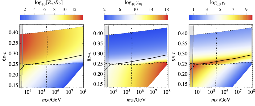
Figure 2: A selection of $(m_{Z^{\prime}},g_{B-L})$ planes, colour-coded according to the ratio of final and initial bubble radii, $R_{*}/R_{0}$ (left), the bubble wall Lorentz factor at which the equilibrium would be reached, $\gamma_{\rm eq}$ (middle) and the bubble wall Lorentz factor at the time of collisions, $\gamma_{*}$ (right). The black curves are the same as in Fig. 1.

As discussed in Ref. [60], an important quantity for the GW calculation is the fraction of the total released energy that is in the scalar field gradients at the bubble wall. Here we improve the calculation of the bubble wall energy presented in Ref. [60]. The bubble wall energy before collisions is

$$E_{\rm wall}=4\pi R^{2}\int_{0}^{R}\frac{{\rm d}R^{\prime}}{3}\big{[}\Delta V-P_{1\to 1}-P_{1\to N}(R^{\prime})\big{]}\,,$$ (4.5)

where the integral gives the surface energy density of the bubble and the prefactor is the area of the bubble surface. The second friction term arising from $1\to N$ splittings depends on the bubble radius through $P_{1\to N}\propto\gamma^{2}=4R^{2}/(9R_{0}^{2})$. For $R>R(\gamma_{\rm eq})$ the integrand is zero and therefore the surface energy density remains constant after the terminal velocity is reached. By defining

$$\alpha_{\infty}=\frac{P_{1\to 1}}{\rho_{R}}\,,$$ (4.6)

we can write the ratio of the bubble wall energy and the total released energy, $E_{V}=4\pi R^{3}\Delta V/3$, which gives the so-called bubble collisions efficiency factor $\kappa_{\rm col}$, as

$$\kappa_{\rm col}=\frac{E_{\rm wall}}{E_{V}}=\begin{cases}\bigg{[}1-\frac{1}{3}\left(\frac{\tilde{\gamma}_{*}}{\gamma_{\rm eq}}\right)^{2}\bigg{]}\bigg{[}1-\frac{\alpha_{\infty}}{\alpha}\bigg{]}\,,&\tilde{\gamma}_{*}<\gamma_{\rm eq}\,,\\ \frac{2}{3}\frac{\gamma_{\rm eq}}{\tilde{\gamma}_{*}}\bigg{[}1-\frac{\alpha_{\infty}}{\alpha}\bigg{]}\,,&\tilde{\gamma}_{*}>\gamma_{\rm eq}\,,\end{cases}$$ (4.7)

where $\tilde{\gamma}_{*}$, defined in Eq. (4.4), is the Lorentz factor that the wall would reach if the friction terms were neglected. Compared to Ref. [60], where the last term in the integrand (4.5) was not accounted for, the main difference is the first factor in the case $\gamma_{*}<\gamma_{\rm eq}$, the absence of which caused a slight overestimation of the bubble wall energy in Ref. [60].

5 Gravitational wave signal

Next we discuss different GW sources in the phase transition. We will start with the GW signal produced by colliding bubbles. While the spectrum from this source can in principle be calculated in a 3D lattice simulation [88, 89, 90], practical realisations are made difficult by the hierarchy between the size of the growing bubble and its very thin wall in strong transitions. As a result it is practically impossible to simulate the strong transitions that would be necessary to produce this signal in realistic scenarios. Because of this, we use results from a simplified approach based on treating walls as infinitely thin shells [91]. Initially these walls were assumed simply to disappear upon collision as the energy dissipates [92, 93, 94]. However, it was recently realised that a more realistic slower dissipation of the source will modify the signal [95, 94]. This leads us to the most recent result [96], which uses the thin-shell approach to compute the GW spectrum while basing the dissipation of the sources on lattice simulations of two-bubble collisions. Following Ref. [96] we calculate the abundance of GWs sourced by the scalar field gradients as

$$\Omega_{{\rm col},*}=2.30\times 10^{-3}\left(R_{*}H_{*}\right)^{2}\left(\frac{\kappa_{\rm col}\alpha}{1+\alpha}\right)^{\!2}\!\left[1+\left(\frac{f}{f_{d}}\right)^{-1.61}\right]\!\left(\frac{f}{f_{{\rm col}}}\right)^{\!2.54}\!\left[1+1.13\left(\frac{f}{f_{{\rm col}}}\right)^{\!2.08}\right]^{-2.30}\!,$$ (5.1)

where the peak frequency is proportional to the inverse of the mean bubble separation,

$$f_{{\rm col}}=0.28R_{*}^{-1}\,,$$ (5.2)

the frequency $f_{d}$ where the low-frequency slope changes is given by

$$f_{d}=0.044R_{*}^{-1}\,,$$ (5.3)

and the efficiency factor $\kappa_{\rm col}$ is given in Eq. (4.7).

We turn next to GW sources related to motions in the primordial plasma, which are typically separated into two distinct periods. First there is the sound wave period observed in numerical lattice simulations involving the relativistic fluid and field bubbles [97, 98, 84]. This behaviour lasts until [84]

$$\tau_{\rm sw}=\frac{R_{*}}{U_{f}}\,,$$ (5.4)

when the fluid motion becomes turbulent and the sound wave period ends . The root-mean- square fluid velocity $U_{f}$ can be approximated as [98]

$$U_{f}\simeq\sqrt{\frac{3}{4}\frac{\alpha_{\rm eff}}{1+\alpha_{\rm eff}}\kappa_{\rm sw}}\,,$$ (5.5)

where $\kappa_{\rm sw}$ is the efficiency coefficient for GW production from sound waves:

$$\kappa_{\rm sw}=\frac{\alpha_{\rm eff}}{\alpha}\frac{\alpha_{\rm eff}}{0.73+0.083\sqrt{\alpha_{\rm eff}}+\alpha_{\rm eff}}\quad,\quad{\rm with}\,\,\,\,\,\alpha_{\rm eff}=\alpha(1-\kappa_{\rm col})\,.$$ (5.6)

GWs are subsequently produced by the ensuing turbulence [100]. Following [60], we assume that at $\tau_{\rm sw}$ all the energy of the fluid motion is simply converted into turbulence, which implies a significant enhancement from this source compared to earlier estimates [101], as the sound wave period generically lasts much less than a Hubble time [81]. The final abundances of the plasma-related sources can be expressed as [101, 60]

$$\Omega_{{\rm sw},*}=0.384\,(\tau_{\rm sw}H_{*})\left(R_{*}H_{*}\right)\left(\frac{\kappa_{\rm sw}\,\alpha}{1+\alpha}\right)^{2}\left(\frac{f}{f_{\rm sw}}\right)^{3}\left[1+\frac{3}{4}\left(\frac{f}{f_{\rm sw}}\right)^{2}\right]^{-\frac{7}{2}}\,,$$ (5.7)

$$\Omega_{{\rm turb},*}=6.85\,\left(R_{*}H_{*}\right)\left(1-\tau_{\rm sw}H_{*}\right)\left(\frac{\kappa_{\rm sw}\,\alpha}{1+\alpha}\right)^{3/2}\frac{\left(\frac{f}{f_{\rm turb}}\right)^{3}\left[1+\left(\frac{f}{f_{\rm turb}}\right)\right]^{-\frac{11}{3}}}{1+8\pi f/H_{*}}\,,$$

with the peak frequencies given by

$$f_{\rm sw}\,\simeq\,3.4R_{*}^{-1}\,,$$ (5.8)

$$f_{\rm turb}\simeq 5.1R_{*}^{-1}\,.$$

In order to compute the final spectra as observed today we also need the appropriate redshift factors, which we discuss at some length in the next Section.

We note that estimates of the plasma-related sources continuously undergo improvements, for instance through analytical description of plasma sound waves [102, 45]. In particular, the modelling of turbulence is far from settled, although much work has been invested in recent years [103, 104, 105, 106, 107, 108, 109, 110]. Pending further developments in modelling these sources, we use the expressions in (5.7) above as representative of the current state of the art most widely used in the community.

Figure 3: A selection of $(m_{Z^{\prime}},g_{B-L})$ planes, colour-coded according to the bubble collisions efficiency factor $\kappa_{\rm col}$, the sound wave efficiency factor $\kappa_{\rm sw}$ and the duration of the sound wave period $\tau_{\rm sw}$. The black curves are the same as in Fig. 1.

We show in Fig. 3 the efficiency factors $\kappa_{\rm col}$ (left panel) and $\kappa_{\rm sw}$ (middle panel), and the duration of the sound wave period $\tau_{\rm sw}$ (right panel) in the classically conformal U$(1)_{B-L}$ model. We see that $\kappa_{\rm col}\sim 1$ below the solid black line where the bubble walls collide before reaching a terminal velocity. This indicates that the GW signal from the phase transition is dominantly sourced by the scalar field gradients. Above that line $\kappa_{\rm col}$ quickly drops and $\kappa_{\rm sw}\sim 1$. In this region the plasma-related sources dominate the GW production. As the duration of the sound wave period in this case is $\tau_{\rm sw}\sim 0.1H_{*}^{-1}$, sound waves and turbulence in the plasma give comparable contributions to the GW signal.

We illustrate the rapid transition from GW signals sourced by plasma motion to scalar field gradients in Fig. 4. To this end we set the U(1)_B-L boson mass to $m_{Z^{\prime}}=3.2\times 10^{5}\,$GeV, and show results for several values of the gauge coupling in the range $0.262\leq g_{B-L}\leq 0.269$. This narrow range is enough to switch from signals dominated by plasma sources to a signal produced predominantly by bubble collisions. We also show the sensitivity of LIGO [63, 64, 65], as well as the projections for the future laser interferometers LISA [66, 67] and Einstein Telescope (ET) [72, 73] and the terrestrial atom interferometer experiment AION [68], its twin project MAGIS [69, 70], and their proposed satellite version AEDGE [71].

Figure 4: Gravitational wave spectra generated in the U(1)_B-L model for $m_{Z^{\prime}}=3.2\times 10^{5}\,$GeV and the range of indicated values of $g_{B-L}$. This range is chosen to exhibit the transition between the bubble collision signals and plasma signals as the gauge coupling increases.

6 Impact of matter domination on the GW signal

We turn now to a discussion of the redshift of the GW signal. We pay special attention to the case in which the very strong transition with $\alpha\gg 1$ is accompanied by very small field decay rate. This causes the field to oscillate around its minimum after the transition, before the Hubble rate drops below the field decay rate to finally allow reheating. If plasma effects can be neglected, these oscillations will dominate the energy density at the end of the transition. If instead the bubble walls reach a terminal velocity before collisions, the energy density after the transition is dominated by the plasma and scales as radiation. However, also in this case the field oscillations can become the dominant energy density component prior to their decay, causing a matter-dominated period.

Accounting for a fraction $1-\kappa_{\rm col}$ of the total released vacuum energy to go into the plasma during the expansion of the bubbles, the energy densities of the scalar field $\varphi$ and radiation at the time of the transition, $t=t_{*}$ are

$$\rho_{\varphi*}=3M_{p}^{2}H_{*}^{2}\frac{\kappa_{\rm col}\alpha}{1+\alpha}\,,\quad\rho_{R*}=3M_{p}^{2}H_{*}^{2}\frac{(1-\kappa_{\rm col})\,\alpha}{1+\alpha}\,.$$ (6.1)

The subsequent decay of the scalar field oscillations into radiation is governed by the $\varphi$ decay rate, $\Gamma_{\varphi}$, and the evolution of the energy densities is governed by the equations

$$\dot{\rho}_{R}+4H\rho_{R}=\Gamma_{\varphi}\rho_{\varphi}\,,\quad\dot{\rho}_{\varphi}+3H\rho_{\varphi}=-\Gamma_{\varphi}\rho_{\varphi}\,,\quad H^{2}=\frac{\rho_{R}+\rho_{\varphi}}{3M_{p}^{2}}\,.$$ (6.2)

It is often convenient to rewrite these equations as functions of the scale factor $a$ rather than time, using ${\rm d}/{\rm d}t=aH{\rm d}/{\rm d}a$. We solve this set of equations numerically, finishing at the scale factor value $a=a_{\times}$ when the contribution of the field becomes negligible: $\rho_{\varphi}(a_{\times})/\rho_{R}(a_{\times})<10^{-3}\kappa_{\rm col}$. To stitch this result together with the subsequent standard radiation-dominated evolution, we simply convert the energy back to temperature via $\rho_{R}(a_{\times})=\pi^{2}g_{*}(T_{\times})T_{\times}^{4}/30$, assuming $g_{*}(T_{\times})\approx 100$ for simplicity.

Whether the field fluctuations decay quickly into radiation or not, the total energy during the transition is the same, and the initial abundance of GWs is not modified significantly [61]. However, after production the GWs redshift in the same way as radiation, and a period of matter domination modifies the GW abundance observed today. The GW spectrum redshifts as

$$\Omega_{{\rm GW},0}(f)=\begin{cases}\left(\frac{a_{*}}{a_{0}}\right)^{4}\left(\frac{H_{*}}{H_{0}}\right)^{2}\Omega_{{\rm GW},*}\!\left(\frac{a_{0}}{a_{*}}f\right)&{\rm for}\quad f>f_{*}\,,\\ \left(\frac{a_{f}}{a_{0}}\right)^{4}\left(\frac{H_{f}}{H_{0}}\right)^{2}\Omega_{{\rm GW},*}\!\left(\frac{a_{0}}{a_{*}}f_{*}\right)\left(\frac{f}{f_{*}}\right)^{3}&{\rm for}\quad f<f_{*}\,,\end{cases}$$ (6.3)

where $a_{f}$ corresponds to the scale factor when the scale $2\pi f$ re-enters the horizon, $2\pi f=a_{f}H_{f}$, and $2\pi f_{*}=a_{*}H_{*}$ corresponds to the horizon-size wavelength at the time of the phase transition. We can write the redshift factor for the total abundance as

$$\left(\frac{a}{a_{0}}\right)^{4}\left(\frac{H}{H_{0}}\right)^{2}=1.67\times 10^{-5}h^{-2}\left(\frac{100}{g_{\rm eff}(T_{\times})}\right)^{\frac{1}{3}}\left(\frac{a}{a_{\times}}\right)^{4}\left(\frac{H}{H_{\times}}\right)^{2}\,,$$ (6.4)

and for the frequency as

$$\frac{a_{0}}{a_{*}}=2.70\times 10^{15}\left(\frac{T_{\times}}{100\,{\rm GeV}}\right)\left(\frac{g_{\rm eff}(T_{\times})}{100}\right)^{\frac{1}{3}}\frac{a_{\times}}{a_{*}}\,.$$ (6.5)

In addition to redshifting the peak of the spectrum, another important effect is that a matter-dominated period can produce features in the spectrum, as superhorizon modes re-entering the horizon at different times get different redshift factors [62]. Beyond the horizon size at the time of production, the spectrum from a short-lasting source, such as a phase transition, is $\propto f^{3}$ in standard radiation-dominated expansion [111, 112], but the behaviour changes to $\propto f^{1}$ for scales re-entering the horizon during matter domination [113]. Therefore, during a matter-dominated period we observe a tilted ‘plateau’ with slope $f^{1}$ developing below the frequency corresponding to the horizon size. The length of this plateau is dictated by the length of the matter-dominated period, which is given in our model by $\Gamma_{\varphi}/H_{*}$. We illustrate this effect in Fig. 5 by showing the GW spectra for a few chosen points in the parameter space with different values of $\Gamma_{\varphi}/H_{*}$. As we see, for smaller decay rates the overall abundance of the spectrum is diminished across much of the spectrum by the modified redshifting, whereas the flatter ‘plateau’ at small frequencies becomes longer. In this example, the ‘plateau’ may be measurable by LISA, whereas the peak might be detectable by AEDGE as well as LISA.

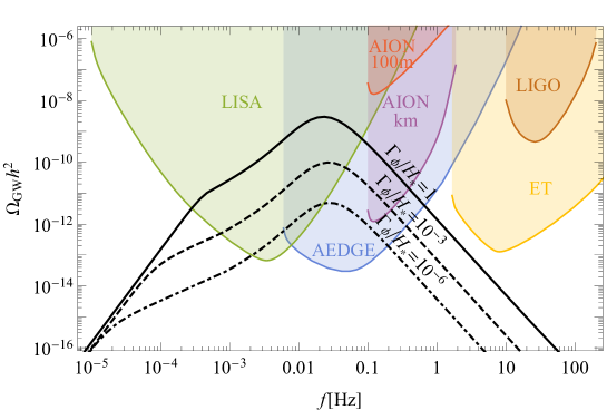
Figure 5: GW spectra generated by bubble collisions for $g_{B-L}=0.26$ and selected values of $m_{Z^{\prime}}=3\times 10^{5}\,$GeV (solid) $m_{Z^{\prime}}=8\times 10^{5}\,$GeV (dashed) $m_{Z^{\prime}}=2\times 10^{6}\,$GeV (dot-dashed) in the U(1)_B-L model. The corresponding values of $\Gamma_{\varphi}/H_{*}$ are also indicated above the signals. The period of matter-dominated expansion elongates the inclined ‘plateau’ below the peak in the frequency spectrum, and also suppresses the peak as $m_{Z^{\prime}}$ increases.

This effect can be also described with a simple analytical approximation in the case that at $a=a_{*}$ the scalar field oscillations dominate the energy density, $\rho_{\varphi*}\gg\rho_{R*}$. We start by approximating to the solution of the system (6.2) to describe the brief period of matter domination as [62]

$$H(a)=H_{*}\left(\frac{a_{*}}{a_{\rm reh}}\right)^{\frac{3}{2}}\left(\frac{a_{\rm reh}}{a}\right)^{2}\left[1+\left(\frac{a_{\rm reh}}{a}\right)^{2}\right]^{-\frac{1}{4}}\,.$$ (6.6)

For this approximation to work properly it is crucial to find the value of the scale factor $a_{\rm reh}$ at which radiation domination resumes. Assuming that the expansion is dominated by field oscillations from $H_{*}$ we get

$$t-t_{*}=\int_{a_{*}}^{a}\frac{{\rm d}a}{aH}=\frac{2}{3}\frac{1}{H_{*}}\left[\left(\frac{a}{a_{*}}\right)^{\frac{3}{2}}-1\right],$$ (6.7)

which, combined with the lifetime of the oscillations given by $\tau_{\varphi}=1/\Gamma_{\varphi}$, and assuming that $\Gamma_{\varphi}\ll H_{*}$, gives

$$a_{\rm reh}=a_{*}\left(\frac{3}{2}\frac{H_{*}}{\Gamma_{\varphi}}\right)^{\frac{2}{3}}\,.$$ (6.8)

In order to implement modifications to the GW signal we find the frequency corresponding to the horizon size at reheating, $f_{H{\rm reh}}=a_{\rm reh}H(a_{\rm reh})/2\pi$, and the frequency corresponding to the horizon size at transition, $f_{*}=a_{*}H(a_{*})/2\pi$. We can then use Eq. (6.6) to solve for the evolution of the scale factor

$$\frac{a}{a_{\rm reh}}=\sqrt{\frac{\chi(f)}{2}-\frac{1}{2}}\,,\quad\chi(f)\equiv\sqrt{8\left(\frac{f_{H{\rm reh}}}{f}\right)^{4}+1}\,.$$ (6.9)

The final step is to use this while taking care of the terms in Eq. (6.3) corresponding to redshifting up to $a_{\rm reh}$, obtaining

$$\left(\frac{a}{a_{\rm reh}}\right)^{4}\left(\frac{H}{H_{\rm reh}}\right)^{2}\approx\begin{cases}1&{\rm for}\quad f<f_{H{\rm reh}}\,,\\ \sqrt{2\frac{\chi(f)-1}{\chi(f)+1}}&{\rm for}\quad f_{H{\rm reh}}<f<f_{*}\,,\\ \sqrt{2\frac{\chi(f_{*})-1}{\chi(f_{*})+1}}&{\rm for}\quad f>f_{*}\,,\end{cases}$$ (6.10)

where the frequency dependence and various cases take into account the redshifting of modes only after they re-enter the horizon.

We have checked this approximation against our numerical results, finding that it is quite accurate provided that $\Gamma_{\varphi}/H_{*}\ll 1$ and $\kappa_{\rm col}\approx 1$, in which case it can easily be used to reproduce the $f^{1}$ plateau developing in the GW spectrum at low frequencies. However, we still use the full numerical result of Eq. (6.2) in the results we show in the next Section, partly due to one additional caveat, namely that, even if $\kappa_{\rm col}$ in Eq. (6.1) is small and significant reheating occurs at the transition, the small amount of energy stored in field oscillations can still dominate the expansion for some time after the transition if the dominant radiation redshifts away before the field decay overtakes the expansion rate. In that case the additional plateau loses significance, as it is far detached from the peak, though the additional redshift can still make the spectra more difficult to observe. 

7 Prospects for observing the GW signals

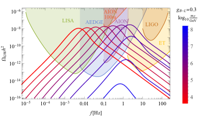
Figure 6: GW spectra for selected values of $g_{B-L}=0.22$ (left panel) and $0.3$ (right panel), and of $m_{Z^{\prime}}$ (colour-coded) in the U(1)_B-L model, calculated for the values of $\Gamma_{\varphi}/H_{*}$ given by Eq. (3.11). The period of matter-dominated expansion causes the tilted ‘plateau’ below the peak in the frequency spectrum, and also the suppression of the peak for larger $m_{Z^{\prime}}$.

We display in Fig. 6 the spectra of GWs for $g_{B-L}=0.22$ (left panel) and $g_{B-L}=0.30$ (right panel) and selected values of $m_{Z^{\prime}}$ indicated by colour coding. Plasma sources of GWs such as sound waves and turbulence dominate the signal for $g_{B-L}=0.3$, whereas for $g_{B-L}=0.22$ the spectra are predominantly produced through bubble collisions. In both panels, the leftmost spectrum is that for the lightest $Z^{\prime}$ boson consistent with LHC data, with a mass, $m_{Z^{\prime}}\simeq 4\,$TeV. The damping of the signal visible at high masses is due to the modified redshifting of the signal caused by very slow decay of the field, which leads to a period of matter domination. This effect is more severe if initially most of the energy is stored in the scalar field profiles, as in the left panel, and we see that the signals are diminished before they reach ET frequencies. The same effect is visible in the right panel, although the matter-domination period there is postponed due to significant reheating during the transition and, as a result, higher peak frequencies are populated. The visible effect of this matter-domination period is the lengthening of the $\propto f^{1}$ ‘plateau’ forming at frequencies below the peak in the lower spectra in the left panel. The same feature appears also in the right panel. However, because the matter-domination period begins significantly after the transition for this larger value of $g_{B-L}$, the feature appears much further from the peak and is not apparent in the figure. We see that when $g_{B-L}=0.22$ in this model the LHC lower limit on $m_{Z^{\prime}}$ reduces the chances for detection of a GW signal by LISA [66, 67], and that the suppression by matter domination of the peak for large $m_{Z^{\prime}}$ appears to preclude measurement of this GW signal by ET [72, 73]. On the other hand, AEDGE [71] appears to offer good prospects for GW detection for $m_{Z^{\prime}}\lesssim 10^{6}\,$GeV and AION 1km [68] also has some prospects for $m_{Z^{\prime}}\sim 10^{6}\,$TeV. On the other hand, when $g_{B-L}=0.3$ each of LISA, AEDGE and ET has a good prospect for GW detection over some range of $m_{Z^{\prime}}$, as does AION 1km, and even AION 100m has some prospects for $m_{Z^{\prime}}\sim 10^{6}\,$TeV, though detection by LIGO [63, 64, 65] appears difficult.

Figure 7: The expected signal-to-noise ratio (SNR) for observing the stochastic GW background from the U(1)_B-L breaking phase transition for different future experiments: LISA (top left), AION 100m (top right), AION 1km (middle left), AEDGE (middle right), LIGO (bottom left), and ET (bottom right). In the red regions ${\rm SNR}>1000$ and in the blue regions ${\rm SNR}<0.001$. The solid gray contours correspond to ${\rm SNR}=10$, and the dashed gray contour in the bottom left panel indicates ${\rm SNR}=1$ for the current LIGO sensitivity. Below the black solid curves the bubbles collide before they reach terminal velocity and the signal is dominated by the contribution from scalar field gradients, while above that line plasma-related sources dominate.

Our next step is to probe systematically the parameter space for GW detection prospects in the various experiments. To this end, we make a standard signal-to-noise ratio (SNR) analysis. For each experiment we use its noise curve to calculate the SNR for the spectrum predicted at each point in the parameter space using

$${\rm SNR}\equiv\sqrt{\mathcal{T}\int{\rm d}f\,\left[\frac{\Omega_{\rm GW}(f)}{\Omega_{\rm noise}(f)}\right]^{2}}\,,$$ (7.1)

where we assume operation for a period $\mathcal{T}=4$ yr for each experiment. We display the results in Fig. 7 for six experiments: LISA, AION 100m, AION 1km, AEDGE, LIGO and ET. In the case of LIGO we show its design sensitivity. The current sensitivity does not reach ${\rm SNR}=10$, but the O2 sensitivity of LIGO reaches ${\rm SNR}>1$ within the region enclosed by the gray dashed contour shown in the upper right panel.

From Fig. 7 we see that LISA (top left panel) has a good reach in the model parameter space, though the spectra in our model are typically pushed to frequencies above the peak sensitivity of LISA, due to collider constraints on the mass $m_{Z^{\prime}}$ of the gauge boson. This means that the mid-frequency band is better suited to this model, and AEDGE and AION 1km (middle panels) can indeed probe a larger part of the allowed model parameter space. Below the solid black line the spectra are mostly produced by bubble collisions, whereas above it plasma-related sources dominate. We see that the effect of matter domination limiting the allowed frequencies from above is especially severe for bubble collision signals and, indeed, prevents ET (bottom right panel) from observing a bubble collision signal with significant SNR. This effect also diminishes the signal at high mass values, but other experiments, especially AEDGE, still have access to a significant part of the parameter space where this signal dominates. The situation is more standard for plasma-related sources where, as usual, larger mass scales are associated with higher frequencies, so LISA probes a lower mass range and ET a higher range, with AION and AEDGE covering the fullest range of frequencies.

8 Conclusions

We have revisited gravitational wave (GW) signals in the U(1)_B-L extension of the Standard Model. We have probed the whole relevant parameter space, paying particular attention to regions with very strong transitions. We find that the GW signals are typically strong and should be detectable in upcoming experiments including LISA, AION/MAGIS, AEDGE, LIGO and ET. The frequency of the signal generically grows with the energy scale of the transition, which is in turn connected to the mass of the new U(1)_B-L $Z^{\prime}$ boson in the model. However, the optimal frequency range is limited from below by constraints on the mass of the the $Z^{\prime}$ boson placed by LHC experiments, and from above by the very slow decay of the U(1)_B-L-breaking field at high masses. This leads to a short matter-domination period that diminishes the signal.

We have refined the calculation of the energy budget for GW sources taking into account the scaling of the friction encountered by bubble walls as $\propto\gamma^{2}$. This means that the walls reach a terminal velocity faster than previously thought and, as a consequence, a smaller fraction of the total energy goes into accelerating the walls. Whilst this does modify the part of the parameter space predicting a strong bubble collision signal, we still find that a large part of the parameter space predicts a strong and potentially observable GW signal sourced predominantly by bubble collisions.

We have scanned the parameter space of the model to identify where the GW signals produced would be within reach of upcoming experiments. We find that LISA as well as AION/MAGIS and AEDGE will be able to observe signals sourced mostly by bubble collision. Observation of such signals at higher frequencies is difficult as the large mass of the field prohibits its decay and triggers a matter-dominated epoch after the transition. This diminishes the signal, and we find that LIGO and ET will not be able to observe bubble collision spectra in our model with a large signal-to-noise ratio. For signals dominated by plasma sources this problem is mitigated, as significant reheating occurs already during the transition. However, even a small fraction of energy initially stored in field oscillations can eventually come to dominate due to its slower redshifting if the field decay is suppressed enough. Nevertheless, signals produced by plasma-related sources extend to much higher frequencies for appropriately large $Z^{\prime}$ boson masses, and they would be observable by LIGO and ET as well as by LISA, AION/MAGIS and AEDGE.

References

- [1] V. A. Kuzmin, V. A. Rubakov and M. E. Shaposhnikov, On the Anomalous Electroweak Baryon Number Nonconservation in the Early Universe, Phys. Lett. B155 (1985) 36.
- [2] A. G. Cohen, D. B. Kaplan and A. E. Nelson, Progress in electroweak baryogenesis, Ann. Rev. Nucl. Part. Sci. 43 (1993) 27 [hep-ph/9302210].
- [3] A. Riotto and M. Trodden, Recent progress in baryogenesis, Ann. Rev. Nucl. Part. Sci. 49 (1999) 35 [hep-ph/9901362].
- [4] D. E. Morrissey and M. J. Ramsey-Musolf, Electroweak baryogenesis, New J. Phys. 14 (2012) 125003 [1206.2942].
- [5] LIGO Scientific, Virgo collaboration, Observation of Gravitational Waves from a Binary Black Hole Merger, Phys. Rev. Lett. 116 (2016) 061102 [1602.03837].
- [6] E. Witten, Cosmic Separation of Phases, Phys. Rev. D30 (1984) 272.
- [7] M. Kamionkowski, A. Kosowsky and M. S. Turner, Gravitational radiation from first order phase transitions, Phys. Rev. D 49 (1994) 2837 [astro-ph/9310044].
- [8] C. Grojean and G. Servant, Gravitational Waves from Phase Transitions at the Electroweak Scale and Beyond, Phys. Rev. D75 (2007) 043507 [hep-ph/0607107].
- [9] J. Espinosa, T. Konstandin, J. No and M. Quiros, Some Cosmological Implications of Hidden Sectors, Phys. Rev. D 78 (2008) 123528 [0809.3215].
- [10] G. C. Dorsch, S. J. Huber and J. M. No, Cosmological Signatures of a UV-Conformal Standard Model, Phys. Rev. Lett. 113 (2014) 121801 [1403.5583].
- [11] J. Jaeckel, V. V. Khoze and M. Spannowsky, Hearing the signal of dark sectors with gravitational wave detectors, Phys. Rev. D94 (2016) 103519 [1602.03901].
- [12] R. Jinno and M. Takimoto, Probing a classically conformal B-L model with gravitational waves, Phys. Rev. D 95 (2017) 015020 [1604.05035].
- [13] M. Chala, G. Nardini and I. Sobolev, Unified explanation for dark matter and electroweak baryogenesis with direct detection and gravitational wave signatures, Phys. Rev. D94 (2016) 055006 [1605.08663].
- [14] M. Chala, M. Ramos and M. Spannowsky, Gravitational wave and collider probes of a triplet Higgs sector with a low cutoff, Eur. Phys. J. C79 (2019) 156 [1812.01901].
- [15] M. Artymowski, M. Lewicki and J. D. Wells, Gravitational wave and collider implications of electroweak baryogenesis aided by non-standard cosmology, JHEP 03 (2017) 066 [1609.07143].
- [16] K. Hashino, M. Kakizaki, S. Kanemura, P. Ko and T. Matsui, Gravitational waves and Higgs boson couplings for exploring first order phase transition in the model with a singlet scalar field, Phys. Lett. B766 (2017) 49 [1609.00297].
- [17] V. Vaskonen, Electroweak baryogenesis and gravitational waves from a real scalar singlet, Phys. Rev. D 95 (2017) 123515 [1611.02073].
- [18] G. Dorsch, S. Huber, T. Konstandin and J. No, A Second Higgs Doublet in the Early Universe: Baryogenesis and Gravitational Waves, JCAP 05 (2017) 052 [1611.05874].
- [19] A. Beniwal, M. Lewicki, J. D. Wells, M. White and A. G. Williams, Gravitational wave, collider and dark matter signals from a scalar singlet electroweak baryogenesis, JHEP 08 (2017) 108 [1702.06124].
- [20] I. Baldes, Gravitational waves from the asymmetric-dark-matter generating phase transition, JCAP 05 (2017) 028 [1702.02117].
- [21] L. Marzola, A. Racioppi and V. Vaskonen, Phase transition and gravitational wave phenomenology of scalar conformal extensions of the Standard Model, Eur. Phys. J. C77 (2017) 484 [1704.01034].
- [22] Z. Kang, P. Ko and T. Matsui, Strong first order EWPT & strong gravitational waves in Z3-symmetric singlet scalar extension, JHEP 02 (2018) 115 [1706.09721].
- [23] S. Iso, P. D. Serpico and K. Shimada, QCD-Electroweak First-Order Phase Transition in a Supercooled Universe, Phys. Rev. Lett. 119 (2017) 141301 [1704.04955].
- [24] M. Chala, C. Krause and G. Nardini, Signals of the electroweak phase transition at colliders and gravitational wave observatories, JHEP 07 (2018) 062 [1802.02168].
- [25] S. Bruggisser, B. Von Harling, O. Matsedonskyi and G. Servant, Electroweak Phase Transition and Baryogenesis in Composite Higgs Models, JHEP 12 (2018) 099 [1804.07314].
- [26] E. Megias, G. Nardini and M. Quiros, Cosmological Phase Transitions in Warped Space: Gravitational Waves and Collider Signatures, JHEP 09 (2018) 095 [1806.04877].
- [27] D. Croon, V. Sanz and G. White, Model Discrimination in Gravitational Wave spectra from Dark Phase Transitions, JHEP 08 (2018) 203 [1806.02332].
- [28] A. Alves, T. Ghosh, H.-K. Guo, K. Sinha and D. Vagie, Collider and Gravitational Wave Complementarity in Exploring the Singlet Extension of the Standard Model, JHEP 04 (2019) 052 [1812.09333].
- [29] P. Baratella, A. Pomarol and F. Rompineve, The Supercooled Universe, JHEP 03 (2019) 100 [1812.06996].
- [30] A. Angelescu and P. Huang, Multistep Strongly First Order Phase Transitions from New Fermions at the TeV Scale, Phys. Rev. D99 (2019) 055023 [1812.08293].
- [31] D. Croon, T. E. Gonzalo and G. White, Gravitational Waves from a Pati-Salam Phase Transition, JHEP 02 (2019) 083 [1812.02747].
- [32] V. Brdar, A. J. Helmboldt and J. Kubo, Gravitational Waves from First-Order Phase Transitions: LIGO as a Window to Unexplored Seesaw Scales, JCAP 1902 (2019) 021 [1810.12306].
- [33] A. Beniwal, M. Lewicki, M. White and A. G. Williams, Gravitational waves and electroweak baryogenesis in a global study of the extended scalar singlet model, JHEP 02 (2019) 183 [1810.02380].
- [34] M. Breitbach, J. Kopp, E. Madge, T. Opferkuch and P. Schwaller, Dark, Cold, and Noisy: Constraining Secluded Hidden Sectors with Gravitational Waves, JCAP 07 (2019) 007 [1811.11175].
- [35] C. Marzo, L. Marzola and V. Vaskonen, Phase transition and vacuum stability in the classically conformal B–L model, Eur. Phys. J. C79 (2019) 601 [1811.11169].
- [36] I. Baldes and C. Garcia-Cely, Strong gravitational radiation from a simple dark matter model, JHEP 05 (2019) 190 [1809.01198].
- [37] T. Prokopec, J. Rezacek and B. Swiezewska, Gravitational waves from conformal symmetry breaking, JCAP 1902 (2019) 009 [1809.11129].
- [38] M. Fairbairn, E. Hardy and A. Wickens, Hearing without seeing: gravitational waves from hot and cold hidden sectors, JHEP 07 (2019) 044 [1901.11038].
- [39] A. J. Helmboldt, J. Kubo and S. van der Woude, Observational prospects for gravitational waves from hidden or dark chiral phase transitions, Phys. Rev. D100 (2019) 055025 [1904.07891].
- [40] P. S. B. Dev, F. Ferrer, Y. Zhang and Y. Zhang, Gravitational Waves from First-Order Phase Transition in a Simple Axion-Like Particle Model, JCAP 1911 (2019) 006 [1905.00891].
- [41] R. Jinno, H. Seong, M. Takimoto and C. M. Um, Gravitational waves from first-order phase transitions: Ultra-supercooled transitions and the fate of relativistic shocks, JCAP 1910 (2019) 033 [1905.00899].
- [42] S. A. R. Ellis, S. Ipek and G. White, Electroweak Baryogenesis from Temperature-Varying Couplings, JHEP 08 (2019) 002 [1905.11994].
- [43] R. Jinno, T. Konstandin and M. Takimoto, Relativistic bubble collisions—a closer look, JCAP 1909 (2019) 035 [1906.02588].
- [44] A. Azatov, D. Barducci and F. Sgarlata, Gravitational traces of broken gauge symmetries, JCAP 07 (2020) 027 [1910.01124].
- [45] M. Hindmarsh and M. Hijazi, Gravitational waves from first order cosmological phase transitions in the Sound Shell Model, JCAP 1912 (2019) 062 [1909.10040].
- [46] B. Von Harling, A. Pomarol, O. Pujolàs and F. Rompineve, Peccei-Quinn Phase Transition at LIGO, 1912.07587.
- [47] L. Delle Rose, G. Panico, M. Redi and A. Tesi, Gravitational Waves from Supercool Axions, JHEP 04 (2020) 025 [1912.06139].
- [48] T. Vachaspati, Magnetic fields from cosmological phase transitions, Phys. Lett. B 265 (1991) 258.
- [49] G. Sigl, A. V. Olinto and K. Jedamzik, Primordial magnetic fields from cosmological first order phase transitions, Phys. Rev. D 55 (1997) 4582 [astro-ph/9610201].
- [50] A. G. Tevzadze, L. Kisslinger, A. Brandenburg and T. Kahniashvili, Magnetic Fields from QCD Phase Transitions, Astrophys. J. 759 (2012) 54 [1207.0751].
- [51] J. Ellis, M. Fairbairn, M. Lewicki, V. Vaskonen and A. Wickens, Intergalactic Magnetic Fields from First-Order Phase Transitions, JCAP 1909 (2019) 019 [1907.04315].
- [52] G. D. Moore and T. Prokopec, How fast can the wall move? A Study of the electroweak phase transition dynamics, Phys. Rev. D52 (1995) 7182 [hep-ph/9506475].
- [53] G. D. Moore and T. Prokopec, Bubble wall velocity in a first order electroweak phase transition, Phys. Rev. Lett. 75 (1995) 777 [hep-ph/9503296].
- [54] D. Bodeker and G. D. Moore, Can electroweak bubble walls run away?, JCAP 05 (2009) 009 [0903.4099].
- [55] J. Kozaczuk, Bubble Expansion and the Viability of Singlet-Driven Electroweak Baryogenesis, JHEP 10 (2015) 135 [1506.04741].
- [56] D. Bodeker and G. D. Moore, Electroweak Bubble Wall Speed Limit, JCAP 05 (2017) 025 [1703.08215].
- [57] G. C. Dorsch, S. J. Huber and T. Konstandin, Bubble wall velocities in the Standard Model and beyond, JCAP 1812 (2018) 034 [1809.04907].
- [58] M. Barroso Mancha, T. Prokopec and B. Swiezewska, Field theoretic derivation of bubble wall force, 2005.10875.
- [59] S. Hoeche, J. Kozaczuk, A. J. Long, J. Turner and Y. Wang, Towards an all-orders calculation of the electroweak bubble wall velocity, 2007.10343.
- [60] J. Ellis, M. Lewicki, J. M. No and V. Vaskonen, Gravitational wave energy budget in strongly supercooled phase transitions, JCAP 1906 (2019) 024 [1903.09642].
- [61] R. Allahverdi et al., The First Three Seconds: a Review of Possible Expansion Histories of the Early Universe, 2006.16182.
- [62] G. Barenboim and W.-I. Park, Gravitational waves from first order phase transitions as a probe of an early matter domination era and its inverse problem, Phys. Lett. B 759 (2016) 430 [1605.03781].
- [63] LIGO Scientific collaboration, Advanced LIGO, Class. Quant. Grav. 32 (2015) 074001 [1411.4547].
- [64] E. Thrane and J. D. Romano, Sensitivity curves for searches for gravitational-wave backgrounds, Phys. Rev. D88 (2013) 124032 [1310.5300].
- [65] LIGO Scientific, Virgo collaboration, GW150914: Implications for the stochastic gravitational wave background from binary black holes, Phys. Rev. Lett. 116 (2016) 131102 [1602.03847].
- [66] N. Bartolo et al., Science with the space-based interferometer LISA. IV: Probing inflation with gravitational waves, JCAP 1612 (2016) 026 [1610.06481].
- [67] C. Caprini, D. G. Figueroa, R. Flauger, G. Nardini, M. Peloso, M. Pieroni et al., Reconstructing the spectral shape of a stochastic gravitational wave background with LISA, JCAP 1911 (2019) 017 [1906.09244].
- [68] L. Badurina et al., AION: An Atom Interferometer Observatory and Network, JCAP 05 (2020) 011 [1911.11755].
- [69] P. W. Graham, J. M. Hogan, M. A. Kasevich and S. Rajendran, Resonant mode for gravitational wave detectors based on atom interferometry, Phys. Rev. D94 (2016) 104022 [1606.01860].
- [70] MAGIS collaboration, Mid-band gravitational wave detection with precision atomic sensors, 1711.02225.
- [71] AEDGE collaboration, AEDGE: Atomic Experiment for Dark Matter and Gravity Exploration in Space, EPJ Quant. Technol. 7 (2020) 6 [1908.00802].
- [72] M. Punturo et al., The Einstein Telescope: A third-generation gravitational wave observatory, Class. Quant. Grav. 27 (2010) 194002.
- [73] S. Hild et al., Sensitivity Studies for Third-Generation Gravitational Wave Observatories, Class. Quant. Grav. 28 (2011) 094013 [1012.0908].
- [74] S. Iso, N. Okada and Y. Orikasa, Classically conformal B–L extended Standard Model, Phys. Lett. B 676 (2009) 81 [0902.4050].
- [75] ATLAS collaboration, Search for new high-mass phenomena in the dilepton final state using 36 fb−1 of proton-proton collision data at sqrt(s)=13 TeV with the ATLAS detector, JHEP 10 (2017) 182 [1707.02424].
- [76] M. Escudero, S. J. Witte and N. Rius, The dispirited case of gauged U(1)B-L dark matter, JHEP 08 (2018) 190 [1806.02823].
- [77] C. Wainwright, S. Profumo and M. J. Ramsey-Musolf, Gravity Waves from a Cosmological Phase Transition: Gauge Artifacts and Daisy Resummations, Phys. Rev. D 84 (2011) 023521 [1104.5487].
- [78] C.-W. Chiang and E. Senaha, On gauge dependence of gravitational waves from a first-order phase transition in classical scale-invariant models, Phys. Lett. B 774 (2017) 489 [1707.06765].
- [79] C. Coriano, L. Delle Rose and C. Marzo, Constraints on abelian extensions of the Standard Model from two-loop vacuum stability and , JHEP 02 (2016) 135 [1510.02379].
- [80] A. D. Linde, Decay of the False Vacuum at Finite Temperature, Nucl. Phys. B216 (1983) 421.
- [81] J. Ellis, M. Lewicki and J. M. No, On the Maximal Strength of a First-Order Electroweak Phase Transition and its Gravitational Wave Signal, JCAP 04 (2019) 003 [1809.08242].
- [82] A. H. Guth and S. H. H. Tye, Phase Transitions and Magnetic Monopole Production in the Very Early Universe, Phys. Rev. Lett. 44 (1980) 631.
- [83] A. H. Guth and E. J. Weinberg, Cosmological Consequences of a First Order Phase Transition in the SU(5) Grand Unified Model, Phys. Rev. D23 (1981) 876.
- [84] M. Hindmarsh, S. J. Huber, K. Rummukainen and D. J. Weir, Shape of the acoustic gravitational wave power spectrum from a first order phase transition, Phys. Rev. D96 (2017) 103520 [1704.05871].
- [85] C. Caprini et al., Detecting gravitational waves from cosmological phase transitions with LISA: an update, JCAP 2003 (2020) 024 [1910.13125].
- [86] M. S. Turner, E. J. Weinberg and L. M. Widrow, Bubble nucleation in first order inflation and other cosmological phase transitions, Phys. Rev. D46 (1992) 2384.
- [87] K. Enqvist, J. Ignatius, K. Kajantie and K. Rummukainen, Nucleation and bubble growth in a first order cosmological electroweak phase transition, Phys. Rev. D45 (1992) 3415.
- [88] H. L. Child and J. T. Giblin, Gravitational Radiation from First-Order Phase Transitions, JCAP 10 (2012) 001 [1207.6408].
- [89] D. Cutting, M. Hindmarsh and D. J. Weir, Gravitational waves from vacuum first-order phase transitions: from the envelope to the lattice, Phys. Rev. D97 (2018) 123513 [1802.05712].
- [90] D. Cutting, E. G. Escartin, M. Hindmarsh and D. J. Weir, Gravitational waves from vacuum first order phase transitions II: from thin to thick walls, 2005.13537.
- [91] A. Kosowsky and M. S. Turner, Gravitational radiation from colliding vacuum bubbles: envelope approximation to many bubble collisions, Phys. Rev. D47 (1993) 4372 [astro-ph/9211004].
- [92] S. J. Huber and T. Konstandin, Gravitational Wave Production by Collisions: More Bubbles, JCAP 0809 (2008) 022 [0806.1828].
- [93] D. J. Weir, Revisiting the envelope approximation: gravitational waves from bubble collisions, Phys. Rev. D 93 (2016) 124037 [1604.08429].
- [94] T. Konstandin, Gravitational radiation from a bulk flow model, JCAP 1803 (2018) 047 [1712.06869].
- [95] R. Jinno and M. Takimoto, Gravitational waves from bubble dynamics: Beyond the Envelope, JCAP 01 (2019) 060 [1707.03111].
- [96] M. Lewicki and V. Vaskonen, Gravitational wave spectra from strongly supercooled phase transitions, 2007.04967.
- [97] M. Hindmarsh, S. J. Huber, K. Rummukainen and D. J. Weir, Gravitational waves from the sound of a first order phase transition, Phys. Rev. Lett. 112 (2014) 041301 [1304.2433].
- [98] M. Hindmarsh, S. J. Huber, K. Rummukainen and D. J. Weir, Numerical simulations of acoustically generated gravitational waves at a first order phase transition, Phys. Rev. D92 (2015) 123009 [1504.03291].
- [99] H.-K. Guo, K. Sinha, D. Vagie and G. White, Phase Transitions in an Expanding Universe: Stochastic Gravitational Waves in Standard and Non-Standard Histories, 2007.08537.
- [100] C. Caprini, R. Durrer and G. Servant, The stochastic gravitational wave background from turbulence and magnetic fields generated by a first-order phase transition, JCAP 0912 (2009) 024 [0909.0622].
- [101] C. Caprini et al., Science with the space-based interferometer eLISA. II: Gravitational waves from cosmological phase transitions, JCAP 1604 (2016) 001 [1512.06239].
- [102] M. Hindmarsh, Sound shell model for acoustic gravitational wave production at a first-order phase transition in the early Universe, Phys. Rev. Lett. 120 (2018) 071301 [1608.04735].
- [103] C. Caprini and R. Durrer, Gravitational waves from stochastic relativistic sources: Primordial turbulence and magnetic fields, Phys. Rev. D74 (2006) 063521 [astro-ph/0603476].
- [104] T. Kahniashvili, L. Kisslinger and T. Stevens, Gravitational Radiation Generated by Magnetic Fields in Cosmological Phase Transitions, Phys. Rev. D 81 (2010) 023004 [0905.0643].
- [105] T. Kahniashvili, A. G. Tevzadze and B. Ratra, Phase Transition Generated Cosmological Magnetic Field at Large Scales, Astrophys. J. 726 (2011) 78 [0907.0197].
- [106] T. Kahniashvili, A. G. Tevzadze, A. Brandenburg and A. Neronov, Evolution of Primordial Magnetic Fields from Phase Transitions, Phys. Rev. D 87 (2013) 083007 [1212.0596].
- [107] T. Kahniashvili, A. Brandenburg, L. Campanelli, B. Ratra and A. G. Tevzadze, Evolution of inflation-generated magnetic field through phase transitions, Phys. Rev. D 86 (2012) 103005 [1206.2428].
- [108] P. Niksa, M. Schlederer and G. Sigl, Gravitational Waves produced by Compressible MHD Turbulence from Cosmological Phase Transitions, Class. Quant. Grav. 35 (2018) 144001 [1803.02271].
- [109] A. Roper Pol, S. Mandal, A. Brandenburg, T. Kahniashvili and A. Kosowsky, Numerical Simulations of Gravitational Waves from Early-Universe Turbulence, 1903.08585.
- [110] J. Ellis, M. Fairbairn, M. Lewicki, V. Vaskonen and A. Wickens, Detecting circular polarisation in the stochastic gravitational-wave background from a first-order cosmological phase transition, 2005.05278.
- [111] C. Caprini, R. Durrer, T. Konstandin and G. Servant, General Properties of the Gravitational Wave Spectrum from Phase Transitions, Phys. Rev. D 79 (2009) 083519 [0901.1661].
- [112] R.-G. Cai, S. Pi and M. Sasaki, Universal infrared scaling of gravitational wave background spectra, 1909.13728.
- [113] G. Domènech, S. Pi and M. Sasaki, Induced gravitational waves as a probe of thermal history of the universe, 2005.12314.